Explaining Residential Ethnic Segregation in the Netherlands using Price Hedonics

Cheng Boon OngHSA-ECS Workshop 15 April 2010

Presentation Outline

1. Context2. Price Hedonic Method3. Data and specification4. 1st stage semiparametric5. 3rd stage: heterogeneous preference

for neighbourhood ethnic composition

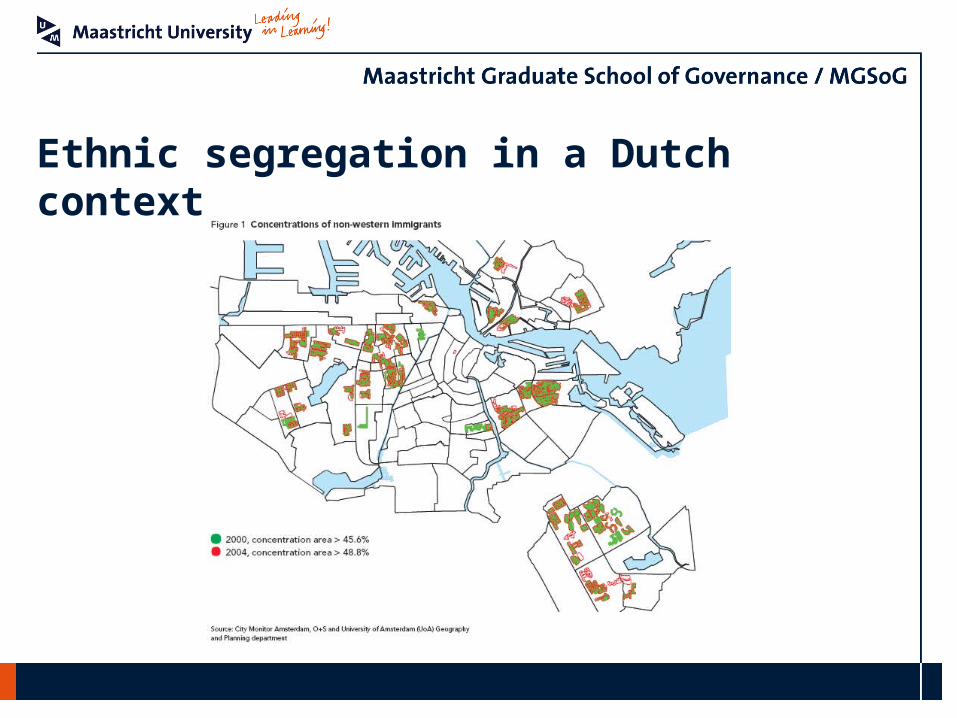
Ethnic segregation in a Dutch context

Native Non-western Western Total

Homeownership 59.20 22.65 42.79 54.53

Social rental 30.59 66.32 42.89 34.84

Private rental 8.25 9.02 12.40 8.67

Median indoor floor space (m2) 127.39 86.37 109.94 122.23

Average net rent (€/month) 368.97 329.87 386.33 364.80

Average WOZ dwelling price (€ ‘000) 211.91 149.32 193.36 204.70

Big City (Randstad) 11.51 42.84 21.69 15.26

Other municipalities 88.49 57.16 78.31 84.74

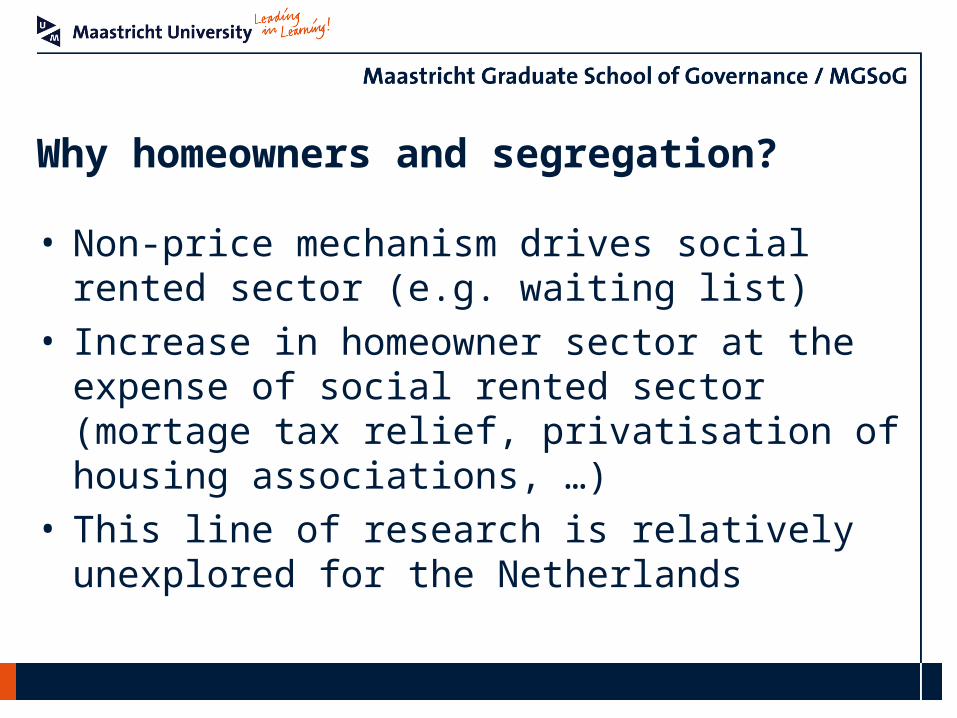
Why homeowners and segregation?

• Non-price mechanism drives social rented sector (e.g. waiting list)

• Increase in homeowner sector at the expense of social rented sector (mortage tax relief, privatisation of housing associations, …)

• This line of research is relatively unexplored for the Netherlands

Price Hedonic Method

• Real estate valuation, transaction data• Microeconomic consumer choice theory

(utility, budget constraint, …)• Housing as a bundle of separable attributes

with unique subutility components and implicit prices for each attribute (Lancaster 1966, Rosen 1974)

• Bajari and Kahn (2005): heterogeneous preferences

Bajari and Kahn (2005) three-stage

• 1st stage: estimate implicit prices for each housing attribute (semiparametric GAM)

• 2nd stage: recover household preference parameter with 1st stage coefficients and observed housing attributes

• 3rd stage: estimate joint distribution of preferences and household characteristics

Utility of household i consuming dwelling j with housing attributes, k:uij = u(xj, ξj, c)

= βi,kln(xj) + βi,kxj + βi,jln(ξj) + c

Household preference for attribute k, βi,k = xj*,k(∂p(xj*, ξj*)/∂xj,k)

…as a function of household characteristics, zβi,k = fk(zi) + εi,k

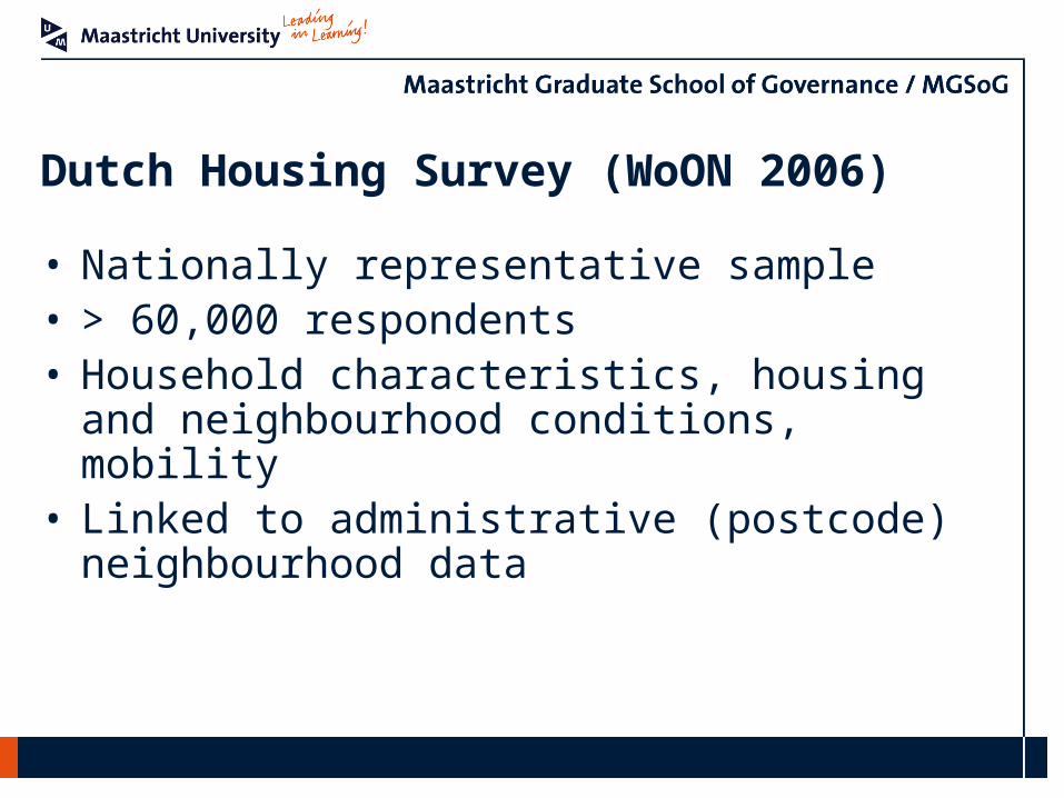
Dutch Housing Survey (WoON 2006)

• Nationally representative sample• > 60,000 respondents• Household characteristics, housing and

neighbourhood conditions, mobility• Linked to administrative (postcode)

neighbourhood data

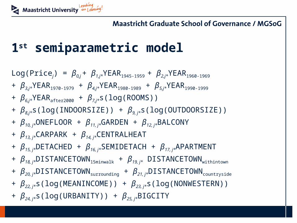
1st semiparametric model

Log(Pricej) = β0,j + β1,j*YEAR1945-1959 + β2,j*YEAR1960-1969

+ β3,j*YEAR1970-1979 + β4,j*YEAR1980-1989 + β5,j*YEAR1990-1999

+ β6,j*YEARafter2000 + β7,j*s(log(ROOMS))

+ β8,j*s(log(INDOORSIZE)) + β9, j*s(log(OUTDOORSIZE))

+ β10, j*ONEFLOOR + β11, j*GARDEN + β12, j*BALCONY

+ β13, j*CARPARK + β14, j*CENTRALHEAT

+ β15, j*DETACHED + β16, j*SEMIDETACH + β17, j*APARTMENT

+ β18, j*DISTANCETOWN15minwalk + β19, j* DISTANCETOWNwithintown

+ β20, j*DISTANCETOWNsurrounding + β21, j*DISTANCETOWNcountryside

+ β22, j*s(log(MEANINCOME)) + β23, j*s(log(NONWESTERN))

+ β24, j*s(log(URBANITY)) + β25, j*BIGCITY

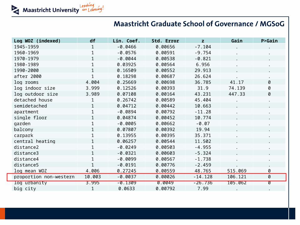
Log WOZ (indexed) df Lin. Coef. Std. Error z Gain P>Gain1945-1959 1 -0.0466 0.00656 -7.104 . .1960-1969 1 -0.0576 0.00591 -9.754 . .1970-1979 1 -0.0044 0.00538 -0.821 . .1980-1989 1 0.03925 0.00564 6.956 . .1990-2000 1 0.16509 0.00552 29.913 . .after 2000 1 0.18298 0.00687 26.624 . .log rooms 4.004 0.25669 0.00698 36.785 41.17 0log indoor size 3.999 0.12526 0.00393 31.9 74.139 0log outdoor size 3.989 0.07108 0.00164 43.231 447.33 0detached house 1 0.26742 0.00589 45.404 . .semidetached 1 0.04712 0.00442 10.663 . .apartment 1 -0.0894 0.00792 -11.28 . .single floor 1 0.04874 0.00452 10.774 . .garden 1 -0.0005 0.00662 -0.07 . .balcony 1 0.07807 0.00392 19.94 . .carpark 1 0.13955 0.00395 35.371 . .central heating 1 0.06257 0.00544 11.502 . .distance2 1 -0.0249 0.00503 -4.955 . .distance3 1 -0.0321 0.00603 -5.324 . .distance4 1 -0.0099 0.00567 -1.738 . .distance5 1 -0.0191 0.00776 -2.459 . .log mean WOZ 4.006 0.27245 0.00559 48.765 515.069 0proportion non-western 10.003 -0.0037 0.00026 -14.128 106.121 0log urbanity 3.995 -0.1309 0.0049 -26.736 105.062 0big city 1 0.0633 0.00792 7.99 . .

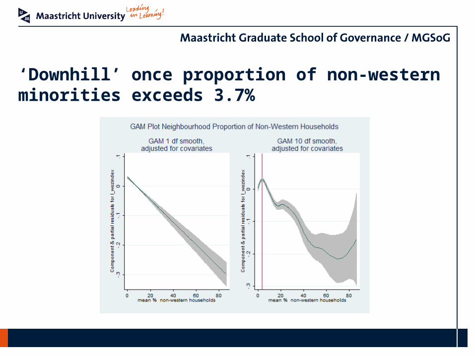
‘Downhill’ once proportion of non-western minorities exceeds 3.7%

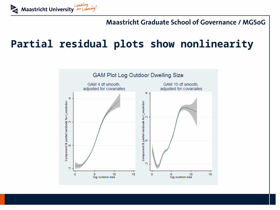
Partial residual plots show nonlinearity

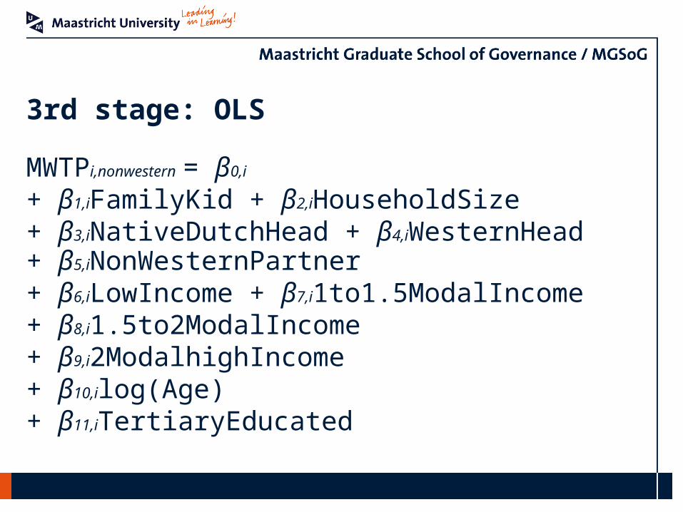
3rd stage: OLS

MWTPi,nonwestern = β0,i + β1,iFamilyKid + β2,iHouseholdSize + β3,iNativeDutchHead + β4,iWesternHead + β5,iNonWesternPartner

+ β6,iLowIncome + β7,i1to1.5ModalIncome+ β8,i1.5to2ModalIncome + β9,i2ModalhighIncome+ β10,ilog(Age)+ β11,iTertiaryEducated

Calculate Marginal Willingness to Pay

MWTPnonwestern10-35%increase,i = βi,k*(10) - βi,k*(35)

MWTPnonwestern0-3%increase,i = βi,k*(3) - βi,k*(0)

MWTP 10% to 35% non-western Coef. Std. Err. t P>t [95% Conf. Interval]

Family with kids 0.0745 0.7296 0.1000 0.9190 -1.3556 1.5045

# household members -1.4839 0.3020 -4.9100 0.0000 -2.0759 -0.8920

Western minority -19.1146 1.3957 -13.7000 0.0000 -21.8504 -16.3789

Native Dutch -21.8883 1.2169 -17.9900 0.0000 -24.2734 -19.5031

< Social minimum -1.6483 1.4538 -1.1300 0.2570 -4.4979 1.2012

1-1.5 Model income -0.4339 0.8502 -0.5100 0.6100 -2.1003 1.2326

1.5-2 Modal income -1.3046 0.8411 -1.5500 0.1210 -2.9532 0.3440

> 2 Modal income -2.1119 0.8179 -2.5800 0.0100 -3.7150 -0.5087

Log age of household head -7.3057 0.7661 -9.5400 0.0000 -8.8072 -5.8042

Tertiary education -0.2726 0.4382 -0.6200 0.5340 -1.1315 0.5863

Non-western partner 24.5194 1.2483 19.6400 0.0000 22.0728 26.9661

constant 60.5632 3.4702 17.4500 0.0000 53.7613 67.3651

Adj R-squared 0.0817          

MWTP 0% to 3% non-western Coef. Std. Err. t P>t [95% Conf. Interval]

Family with kids -0.0089 0.0876 -0.1000 0.9190 -0.1805 0.1627

# household members 0.1781 0.0362 4.9100 0.0000 0.1070 0.2491

Western minority 2.2938 0.1675 13.7000 0.0000 1.9655 2.6220

Native Dutch 2.6266 0.1460 17.9900 0.0000 2.3404 2.9128

< Social minimum 0.1978 0.1745 1.1300 0.2570 -0.1441 0.5398

1-1.5 Model income 0.0521 0.1020 0.5100 0.6100 -0.1479 0.2520

1.5-2 Modal income 0.1566 0.1009 1.5500 0.1210 -0.0413 0.3544

> 2 Modal income 0.2534 0.0981 2.5800 0.0100 0.0610 0.4458

Log age of household head 0.8767 0.0919 9.5400 0.0000 0.6965 1.0569

Tertiary education 0.0327 0.0526 0.6200 0.5340 -0.0704 0.1358

Non-western partner -2.9423 0.1498 -19.6400 0.0000 -3.2359 -2.6487

constant -7.2676 0.4164 -17.4500 0.0000 -8.0838 -6.4514

Adj R-squared 0.0817          

Some preliminary conclusions

• Nonlinear relationship between proportion of non-western households in neighbourhood and dwelling price

• Different demand across ethnicity of household for non-western neighbours – some positive “taste” for non-western neighbours up to a certain level and then the “distaste” sets in

Thank you for your attention!

Comments/suggestions welcome: cheng.ong@maastrichtuniversity.nl