Explaining operational modal analysis with data from an arch bridge

Contents lists available at ScienceDirect

Mechanical Systems and Signal Processing

Mechanical Systems and Signal Processing 25 (2011) 1431–1450

0888-32

doi:10.1

n Corr

E-m

URL

journal homepage: www.elsevier.com/locate/jnlabr/ymssp

Tutorial Review

Explaining operational modal analysis with data from an arch bridge

Filipe Magalh~aes, Alvaro Cunha n

University of Porto, Faculty of Engineering (FEUP), R. Dr. Roberto Frias, 4200-465 Porto, Portugal

a r t i c l e i n f o

Article history:

Received 3 August 2010

Accepted 6 August 2010

70/$ - see front matter & 2010 Elsevier Ltd. A

016/j.ymssp.2010.08.001

esponding author. Tel.: +351 22 508 1580; fa

ail address: [email protected] (A. Cunha).

: http://www.fe.up.pt/vibest (A. Cunha).

a b s t r a c t

This tutorial paper aims to introduce the topic of operational modal analysis to non-

specialists on the subject. First of all, it is stressed the relevance of this experimental

technique particularly in the assessment of important civil infrastructure. Then, after a

synthesis of required theoretical background, three of the most powerful algorithms for

output-only modal identification are presented. The several steps of these identification

procedures are illustrated with the processing of data collected on a concrete arch

bridge with a span of 280 m. As the use of operational modal analysis in the context of

structural health monitoring is a subject under active research, this theme is also

introduced and briefly exemplified with data continuously recorded at the same bridge.

& 2010 Elsevier Ltd. All rights reserved.

Contents

1. Introduction . . . . . . . . . . . . . . . . . . . . . . . . . . . . . . . . . . . . . . . . . . . . . . . . . . . . . . . . . . . . . . . . . . . . . . . . . . . . . . . . . . . . . . . . . 1432

2. Description of the application . . . . . . . . . . . . . . . . . . . . . . . . . . . . . . . . . . . . . . . . . . . . . . . . . . . . . . . . . . . . . . . . . . . . . . . . . . . 1433

3. Theoretical background . . . . . . . . . . . . . . . . . . . . . . . . . . . . . . . . . . . . . . . . . . . . . . . . . . . . . . . . . . . . . . . . . . . . . . . . . . . . . . . . 1434

3.1. Finite element model. . . . . . . . . . . . . . . . . . . . . . . . . . . . . . . . . . . . . . . . . . . . . . . . . . . . . . . . . . . . . . . . . . . . . . . . . . . . 1434

3.2. Stochastic state-space model. . . . . . . . . . . . . . . . . . . . . . . . . . . . . . . . . . . . . . . . . . . . . . . . . . . . . . . . . . . . . . . . . . . . . . 1434

3.3. Transfer function . . . . . . . . . . . . . . . . . . . . . . . . . . . . . . . . . . . . . . . . . . . . . . . . . . . . . . . . . . . . . . . . . . . . . . . . . . . . . . . 1436

3.4. Modal model . . . . . . . . . . . . . . . . . . . . . . . . . . . . . . . . . . . . . . . . . . . . . . . . . . . . . . . . . . . . . . . . . . . . . . . . . . . . . . . . . . 1436

3.5. Right matrix fraction model . . . . . . . . . . . . . . . . . . . . . . . . . . . . . . . . . . . . . . . . . . . . . . . . . . . . . . . . . . . . . . . . . . . . . . 1437

3.6. Output spectrum and half-spectrum. . . . . . . . . . . . . . . . . . . . . . . . . . . . . . . . . . . . . . . . . . . . . . . . . . . . . . . . . . . . . . . . 1437

4. Modal parameters identification . . . . . . . . . . . . . . . . . . . . . . . . . . . . . . . . . . . . . . . . . . . . . . . . . . . . . . . . . . . . . . . . . . . . . . . . . 1438

4.1. Overview of OMA methods . . . . . . . . . . . . . . . . . . . . . . . . . . . . . . . . . . . . . . . . . . . . . . . . . . . . . . . . . . . . . . . . . . . . . . . 1438

4.2. Pre-processing . . . . . . . . . . . . . . . . . . . . . . . . . . . . . . . . . . . . . . . . . . . . . . . . . . . . . . . . . . . . . . . . . . . . . . . . . . . . . . . . . 1439

4.3. FDD and EFDD . . . . . . . . . . . . . . . . . . . . . . . . . . . . . . . . . . . . . . . . . . . . . . . . . . . . . . . . . . . . . . . . . . . . . . . . . . . . . . . . . 1440

4.4. SSI-COV . . . . . . . . . . . . . . . . . . . . . . . . . . . . . . . . . . . . . . . . . . . . . . . . . . . . . . . . . . . . . . . . . . . . . . . . . . . . . . . . . . . . . . 1442

4.5. p-LSCF. . . . . . . . . . . . . . . . . . . . . . . . . . . . . . . . . . . . . . . . . . . . . . . . . . . . . . . . . . . . . . . . . . . . . . . . . . . . . . . . . . . . . . . . 1444

5. Automated operational modal analysis . . . . . . . . . . . . . . . . . . . . . . . . . . . . . . . . . . . . . . . . . . . . . . . . . . . . . . . . . . . . . . . . . . . 1447

6. Conclusions . . . . . . . . . . . . . . . . . . . . . . . . . . . . . . . . . . . . . . . . . . . . . . . . . . . . . . . . . . . . . . . . . . . . . . . . . . . . . . . . . . . . . . . . . 1449

References . . . . . . . . . . . . . . . . . . . . . . . . . . . . . . . . . . . . . . . . . . . . . . . . . . . . . . . . . . . . . . . . . . . . . . . . . . . . . . . . . . . . . . . . . . 1449

ll rights reserved.

x: +351 22 508 1835

www.elsevier.com/locate/jnlabr/ymssp

dx.doi.org/10.1016/j.ymssp.2010.08.001

mailto:[email protected]

mailto:http://www.fe.up.pt/vibest.3d

dx.doi.org/10.1016/j.ymssp.2010.08.001

F. Magalh ~aes, A. Cunha / Mechanical Systems and Signal Processing 25 (2011) 1431–14501432

1. Introduction

Experimental identification of modal parameters is a research topic with more than six decades of history. Itstarted to be applied in Mechanical Engineering to characterize the dynamic behaviour of relatively small structurestested in a controlled environment, inside a laboratory. This first approach, nowadays called experimental modalanalysis (EMA), is based on the performance of forced vibration tests (FVT), involving the simultaneous measurementof one or more dynamic excitations and the corresponding structural response. From the relation between theapplied input and the observed output, it is possible to accurately identify modal parameters. Since the first practicalapplications until now, the testing equipment and the algorithms for data processing have evolved significantly. Therefore,EMA is currently a well-established field founded on solid theoretical bases extensively documented in reference books[1–3] and largely used in practice, particularly in aerospace and automotive industries. Several relevant applicationsare documented in the issues of the Mechanical System and Signal Processing Journal (MSSP) published during thelast 25 years and in the proceedings of the International Modal Analysis Conference (IMAC), an annual conferenceorganized since 1982.

EMA techniques can also be adopted for identification of modal parameters of Civil Engineering structures, like bridges,dams or buildings. Though, their large size imposes additional challenges. In particular, the application of controlled andmeasurable dynamic excitations requires the use of very heavy and expensive devices [4].

Therefore, in the case of Civil Engineering structures, ambient vibration tests (AVT) are much more practical andeconomical, since the artificial excitation produced by heavy shakers is replaced by freely available ambient forces, like thewind or the traffic circulating over or nearby the structure under analysis. As a consequence, AVT have the very relevantadvantage of permitting the dynamic assessment of important civil infrastructure, like bridges, without disturbing theirnormal operation. Furthermore, as structures are characterized using real operation conditions, in case of existence of non-linear behaviour, the obtained results are associated with realistic levels of vibration and not with artificially generatedvibrations, as it is the case when FVT are used.

Also in Mechanical Engineering, operational modal analysis proved to be very useful: for instance to obtain the modalparameters of a car during road testing or of an airplane during flight tests.

Nevertheless, as the level of excitation is low, very sensitive sensors with very low noise levels have to be used and evenso, one should expect much lower signal to noise ratios than the ones observed in traditional tests. Besides this, AVT havetwo additional disadvantages when compared to FVT: the frequency content of the excitation may not cover the wholefrequency band of interest, especially in the case of very stiff structures with high natural frequencies, and modal massesare not estimated, or mode shapes are not scaled in absolute sense, unless additional tests with extra masses over thestructure are performed [5].

As with ambient vibration tests the modal information is derived from structural responses (outputs) while thestructure is in operation, this identification process is usually called operational modal analysis (OMA) or output-onlymodal analysis (in opposition to input–output modal analysis). As the knowledge of the input is replaced by theassumption that the input is a realization of a stochastic process (white noise), the determination of a model that fits themeasured data is also named stochastic system identification.

The modal properties provided by the application of operational modal analysis are useful to check, and if necessaryupdate, numerical models of new structures, to tune vibration control devices that might have been adopted, to evaluatethe safety of existing structures in the context of inspection programs, to characterize existent structures before thedevelopment of rehabilitation projects or to obtain a base-line characterization of an existent structure that may be used inthe future as reference to check the evolution of its dynamic characteristics.

The large increase of research activity around the theoretical basis of OMA and its applications has motivated thecreation, in 2005, of the International Operational Modal Analysis Conference (IOMAC) and also the recent edition of aspecial issue of the MSSP Journal [6].

The present paper aims to provide an overview of the theoretical background behind operational modal analysis anddescribe the steps needed for the identification of modal parameters from experimental data. Despite the existence of alarge number of alternative OMA algorithms developed during the last decades, they are however just based on few basicprinciples. Therefore, this work is exclusively focused on the description of three methods with completely distincttheoretical backgrounds, which have also proven to provide very accurate estimates in civil engineering applications:frequency domain decomposition (FDD), covariance driven stochastic subspace identification (SSI-COV) and poly-leastsquares complex frequency domain (p-LSCF). The main operations of the algorithms are illustrated with the processing ofdata collected in a concrete arch bridge.

Therefore, this work starts with a brief description of the full-scale structure used to illustrate the application of theOMA techniques. Then, the presentation of basic theoretical background is followed by the description of the identificationalgorithms. Afterwards, it is provided an introduction to automated modal analysis, a topic under active research due to itsimportance in the context of vibration-based structural health monitoring. Finally, the conclusions also indicate someadditional references especially dedicated to practical applications of operational modal analysis, for broadening anddeepening of the readers’ knowledge.

F. Magalh ~aes, A. Cunha / Mechanical Systems and Signal Processing 25 (2011) 1431–1450 1433

2. Description of the application

The presentation of the algorithms for operational modal analysis is going to be illustrated with the processing ofdatasets collected at the Infante D. Henrique Bridge, a long span concrete arch bridge located in the city of Porto, inPortugal (Fig. 1).

This bridge is composed of two fundamental elements: a very rigid prestressed reinforced concrete box girder, 4.50 mdeep, supported by an extremely shallow and thin reinforced concrete arch, 1.50 m thick, as shown in the elevationrepresented in Fig. 2. The arch spans 280 m between abutments and rises 25 m until the crown. In the 70 m centralsegment, arch and deck meet to define a box-beam 6 m deep. The arch has constant thickness and its width increaseslinearly from 10 m in the central span up to 20 m at the springs [7].

This bridge is equipped with a dynamic monitoring system that comprises 12 acceleration channels, which have beenprogrammed to continuously acquire the bridge response to ambient excitation [8]. The accelerometers are distributed inthe four sections of the bridge deck marked in Fig. 2. Each section is instrumented with three accelerometers: two tomeasure the vertical accelerations at the lateral edges of the deck (characterizing vertical movements and rotations) andanother one to measure lateral accelerations. The system was configured to acquire acceleration signals with a samplingfrequency of 50 Hz and produce time segments with a length of 30 min.

In order to illustrate the application of the identification algorithms described in the next section, the dataset collectedat 23:00 of 22/10/2007 was adopted. For didactic purposes, instead of using the 12 collected time series, the identificationwas just based on the four time series presented in Fig. 3: the average of the two vertical acceleration time series measuredin each instrumented section. The reduction of the amount of data to be processed permits to include more details in theexplanation of the identification techniques.

S1 S2 S3 S4

Fig. 2. Elevation of the bridge showing the instrumented sections: S1–S4.

A1

0 600 1200 1800-1

-0.50

0.511

Time (s)

Acc

eler

atio

n (m

g)

A2

0 600 1200 1800-1

-0.50

0.51

Time (s)

A3

0 600 1200 1800-1

-0.50

0.511

Time (s)

A4

0 600 1200 1800-1

-0.50

0.51

Time (s)

Fig. 3. Average vertical acceleration time series.

Fig. 1. View of Infante D. Henrique Bridge from downstream (Porto at the left side).

f = 0.81 Hz f = 1.14 Hz

f = 1.41 Hz f = 1.99 Hz

Fig. 4. First four identified vertical bending modes.


As a consequence, the obtained results are restricted to the first four vertical bending modes, only characterized by fourmodal components. The achieved estimates can be compared with the ones presented in Fig. 4, which were obtained with avery complete ambient vibration test, described in [8].

3. Theoretical background

The identification of modal parameters is usually performed with the purpose of obtaining accurate experimentalestimates of natural frequencies, mode shapes and modal damping ratios, which can be then correlated with thecorresponding values numerically estimated from a finite element model of the structure under analysis [9].

The majority of the modal identification methods are based on models (called experimental models) of the testeddynamic system that are fitted to the recorded data and from which it is then possible to extract estimates of modalparameters. This section is devoted to the characterization of some alternative experimental models that can be derivedfrom the finite element model.

This subject has already been extensively explored in some reference books [1,10]. So, only the essential conceptsneeded for the understanding of the identification methods described in this paper are presented here. Therefore, emphasiswill be given to models that assume an unknown or stochastic input, as these are the ones used for operational modalanalysis.

3.1. Finite element model

The analysis of a complex dynamic system requires its previous discretization through the construction of a finiteelement model with a finite number of degrees of freedom (n2). After this first step, the equilibrium of such system isrepresented by the following differential equation expressed in matrix form:

M €qðtÞþC1 _qðtÞþKqðtÞ ¼ pðtÞ ¼ B2uðtÞ ð1Þ

where M, C1, K 2 Rn2�n2 are the mass, damping and stiffness matrices; €qðtÞ, _qðtÞ, qðtÞ are time functions organized in columnvectors that characterize the evolution of the acceleration, velocity and displacement of each degree of freedom (each dotover a time function denotes one derivation with respect to time) and pðtÞ is a column vector with the forces applied to thesystem. As normally not all the degrees of freedom (dof) are excited, the load vector with n2 lines can be replaced by avector of inferior dimension (nion2) containing the time evolution of the ni applied inputs. This vector, designated by u(t),is multiplied by a matrix that maps the ni inputs with the n2 dof of the system: B2, a n2-by-ni matrix composed by ones andzeros.

3.2. Stochastic state-space model

The previous second-order system of differential equations can be transformed into a first-order one, the state equation,using simple mathematical manipulations [10]. A state-space model is obtained by combining the state equation with theobservation equation:

_xðtÞ ¼ ACxðtÞþBCuðtÞ

yðtÞ ¼ CCxðtÞþDCuðtÞ ð2Þ

where AC, designated state matrix, is a n-by-n matrix, with n equal to 2n2, and x(t) is the state vector, which contains thedisplacements and the velocities vectors of the dynamic system. The observation equation establishes a relation between asubset of no measured outputs organized in vector y(t) and the ni inputs of dynamic system u(t). CC is the output matrix andDC is designated direct transmission matrix [10].

The modal parameters of the dynamic system can be extracted from the state matrix AC. In [11] it is demonstrated thatthe matrices with the eigenvalues and eigenvectors of AC (LC and C, respectively) have the following structure:

AC ¼CLCC�1


LC ¼L 0

0 L�

� �, C¼

Y Y�

YL Y�L�

" #

L¼

&

lk

&

264

375, Y¼ � � � fk � � �

h i, k¼ 1,:::,n2 ð3Þ

where �� means complex conjugate. The lk are related with the structure frequencies (ok—natural frequencies in rad/s)and modal damping ratios (xk) by the expression:

lk ¼�xkokþ i

ffiffiffiffiffiffiffiffiffiffiffiffiffiffi1�xk

2q

ok ð4Þ

where i¼ffiffiffiffiffiffiffi�1p

.The mode shapes are represented in Eq. (3) by fk. However, as only a subset of the dof is measured, the observable

modal components are given by

F¼ CCC ð5Þ

The number of modes (nm) is equal to the dimension of the finite element model (n2) from which the state-space modelwas derived and equal to one half the dimension of the state-space model: nm=n/2 (n, dimension of the state vector).

In a dynamic test, the analog signals recorded by the transducers are converted to digital data by an analog to digitalconverter (A/D), so that they can be stored and processed by a computer. Therefore, in practice, the available information ofthe dynamic system under study is discrete in time. Consequently, a discrete time version of the previously presentedmodel is more adequate to fit experimental data. Furthermore, in the context of operational modal analysis, the systeminput is unknown. Therefore, the terms of the state-space model in u(t) have to be represented by stochastic components:

xkþ1 ¼ Axkþwk

yk ¼ Cxkþvk ð6Þ

This model is designated discrete-time stochastic state-space model. The time functions x(t) and y(t) are replaced bytheir values at discrete time instants k Dt, where k is an integer and Dt is the adopted sampling interval: xk=x(kDt). Thevectors wk and vk model not only the effect of the unknown outputs, but also the noise due to disturbances and modellinginaccuracies, and the measurement noise due to sensor inaccuracy, respectively. Both vector signals with dimension n areassumed to be zero mean realizations of stochastic processes with the following correlation matrices:

Ewp

vp

" #wp

T vpT

h i !¼

Q S

ST R

� �

Ewp

vp

" #wq

T vqT

h i !¼ 0, paq ð7Þ

where the indexes p and q represent generic time instants and E(�) is the expected value of �. As the correlations matricesof the processes wk and vk, E wpwT

q

� �and E wpwT

q

� �, are assumed to be equal to zero for any time delay t=q�p different

from zero, each new observation of these processes is independent from the previous ones. Such purely random stochasticprocesses are designated white noise processes.

In [10] the expressions that relate the discrete-time model matrices with their continuous-time counterparts arederived. There, it is also demonstrated that the eigenvectors of matrix A coincide with the ones of matrix AC. Theeigenvalues of the discrete model, represented by mk, are related with the ones of the continuous model lk by the followingequation:

mk ¼ elk Dt3lk ¼lnðmkÞ

Dtð8Þ

Consequently, it is proven that once a discrete-time state-space model has been identified from experimental data, it ispossible to estimate the modal parameters of the tested structure. The natural frequencies and model damping ratios areobtained from the eigenvalues of A using Eqs. (8) and (4). Taking into account that C is equal to CC and that the eigenvectorsof A coincide with the eigenvectors of AC, the observable modal components are given by Eq. (5).

Stochastic state-space models present several properties that are essential for the justification of the identificationalgorithms presented later. These are described and proven in [12]. The most important property is the following relationbetween the correlation matrix of the measured structural responses and the state-space matrix:

Rj ¼ CAj�1G ð9Þ

Rj is the correlation matrix of the outputs for any arbitrary time lag t=j Dt and G is the ‘‘next state-output’’ correlationmatrix defined as

G¼ E xkþ1ykT

� �ð10Þ

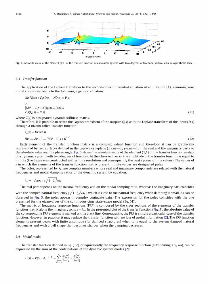
Fig. 5. Absolute value of the element (1,1) of the transfer function of a dynamic system with two degrees of freedom (vertical axis in logarithmic scale).


3.3. Transfer function

The application of the Laplace transform to the second-order differential equation of equilibrium (1), assuming zeroinitial conditions, leads to the following algebraic equation:

Ms2Q ðsÞþC1sQ ðsÞþKQðsÞ ¼ PðsÞ

or

Ms2þC1sþK� �

Q ðsÞ ¼ PðsÞ3

ZðsÞQ ðsÞ ¼ PðsÞ ð11Þ

where Z(s) is designated dynamic stiffness matrix.Therefore, it is possible to relate the Laplace transform of the outputs Q(s) with the Laplace transform of the inputs P(s)

through a matrix called transfer function:

Q ðsÞ ¼HðsÞPðsÞ

HðsÞ ¼ ZðsÞ�1¼ Ms2þC1sþK� ��1

ð12Þ

Each element of the transfer function matrix is a complex valued function and therefore, it can be graphicallyrepresented by two surfaces defined in the Laplace or s-plane (x axis—s; y-axis—io): the real and the imaginary parts orthe absolute value and the phase angle. Fig. 5 shows the absolute value of the element (1,1) of the transfer function matrixof a dynamic system with two degrees of freedom. At the observed peaks, the amplitude of the transfer function is equal toinfinite (the figure was constructed with a finite resolution and consequently the peaks present finite values). The values ofs in which the elements of the transfer function matrix present infinite values are designated poles.

The poles, represented by lk, are complex numbers whose real and imaginary components are related with the naturalfrequencies and modal damping ratios of the dynamic system by equation:

lk ¼�xkokþ i

ffiffiffiffiffiffiffiffiffiffiffiffiffiffi1�xk

2q

ok

The real part depends on the natural frequency and on the modal damping ratio, whereas the imaginary part coincides

with the damped natural frequency (ffiffiffiffiffiffiffiffiffiffiffiffiffiffi1�xk

2q

ok), which is close to the natural frequency when damping is small. As can be

observed in Fig. 5, the poles appear in complex conjugate pairs. The expression for the poles coincides with the onepresented for the eigenvalues of the continuous-time state-space model (Eq. (4)).

The matrix of frequency response functions (FRF) is composed by the cross sections of the elements of the transferfunction matrix along the imaginary axis: s¼ io. In the presented plot of the transfer function (Fig. 5), the absolute value ofthe corresponding FRF element is marked with a black line. Consequently, the FRF is simply a particular case of the transferfunction. However, in practice, it may replace the transfer function with no loss of useful information [2]. The FRF functionelements present peaks with finite amplitude (for damped structures) when o is equal to the system damped naturalfrequencies and with a bell shape that becomes sharper when the damping decreases.

3.4. Modal model

The transfer function defined in Eq. (12), or equivalently the frequency response function (substituting s by io), can beexpressed by the sum of the contributions of the dynamic system modes [2]:

HðsÞ ¼ V sI�Lð Þ�1LT ¼

Xn2

k ¼ 1

fkgTk

s�lkþf�kgH

k

s�l�k


withV ¼ f1 . . . fn2

f1� . . . f�n2

h iL¼ g1 . . . gn2

g�1 . . . g�n2

h i L¼

l1

&

ln2

0

0

l�1&

l�n2

266666666664

377777777775

ð13Þ

where n2 is the number of modes, �� is the complex conjugate of a matrix or vector, �H is the complex conjugate transposeof a matrix or vector, I is a 2n2-by-2n2 identity matrix, fk is a column vector containing the n2 components of mode shapek, gT

k is a line vector with the n2 components of the modal participation factor of mode k and lk, for k=1,y, n2, are thestructure poles.

A transfer function more close to the experimental world should only relate the dof where the inputs are applied withthe measured outputs, and so it is a ni-by-no matrix instead of a n2-by-n2 matrix. In addition, not all the modes areobservable and so the summation is limited to a subset of modes.

3.5. Right matrix fraction model

The modal model is the model in the frequency (or Laplace) domain that provides the best physical understanding froman engineering point of view. However, it is not adequate to be directly fitted to experimental data, as it is highly non-linear. Matrix fraction models (fully described in [13]) are more abstract models that can be more easily fitted to measureddata and then used to obtain estimates of modal parameters.

In particular, the Right Matrix Fraction Model defines the Transfer Function as the right division (B/A) of two polynomialmatrices:

HðsÞ ¼ BðAÞ�1

HðsÞ ¼Xpb

r ¼ 0

Brsr

" # Xpa

r ¼ 0

Arsr

" #�1

ð14Þ

where the matrices Br are no-by-ni and the matrices Ar are ni-by-ni. pa and pb are the orders of the denominator andnumerator polynomials.

Once the model matrices have been estimated, the natural frequencies and the modal damping ratios can be extractedfrom the coefficients of the denominator polynomial and the mode shapes determined from the coefficients of B. Instead, itis also possible to convert the estimated right matrix-fraction model into a state-space model (Eq. (2)). The equationsneeded to make this transposition have been derived in [14], assuming pa=pb=p and that the degree of the polynomial withthe determinant of A(s) is equal to pUni:

AC ¼

�A�1p Ap�1 �A�1

p Ap�2 ::: �A�1p A1 �A�1

p A0

I 0 ::: 0 0

^ & ::: ^ ^

0 0 ::: I 0

26664

37775

BC ¼A�1

p

0

" #

CC ¼ Bp�1�BpA�1p Ap�1 ::: B0�BpA�1

p A0

h iDC ¼ BpA�1

p ð15Þ

After this step, the modal parameters can be estimated from the state-space model matrices, following the procedurepresented in the previous sub-section. As the AC matrix is a square matrix with dimension pni, the model represents adynamic system with pni=2 modes.

3.6. Output spectrum and half-spectrum

In the context of Operational Modal Analysis, the stochastic process used to represent the unknown inputs can becharacterized either by a correlation matrix (as in Eq. (7)) or by a matrix with the input spectra (Laplace transforms of theinput correlations).

The output spectrum matrix Syy, restricted to s¼ io, is related with the input spectrum matrix Suu by the followingequation [15]:

SyyðoÞ ¼HðoÞSuuðoÞHHðoÞ ð16Þ


In the particular case where the input is assumed to be a white noise, the output spectrum only depends on the systemtransfer function H(o) and on a constant matrix that coincides with the white noise input correlation matrix:

SyyðoÞ ¼HðoÞRuuHHðoÞ ð17Þ

Taking into account the modal decomposition of the transfer function (Eq. (13)), it is also possible to express the outputspectrum as a superposition of the contribution of the structure modes. Considering the contribution of all the systemmodes (n2), the following equation is obtained [11]:

SyyðoÞ ¼Xn2

k ¼ 1

fkgTk

io�lkþ

f�kgHk

io�l�kþ

gkfTk

�io�lkþ

g�kfHk

�io�l�kð18Þ

where the vectors gk, called operational reference vectors, take the place of the modal participation factors. However, thesevectors do not depend only on the characteristics of mode k. As proven in [11], each gk depends on all the structure modalparameters, on the input locations and on the input correlation matrix.

The modal decomposition of the output spectrum shows that this has four poles (lk, �lk, l�k and �l�k) for each mode.This imposes the use of models with orders that are twice the model order needed to model the transfer function of thesame dynamic system. This disadvantage can be avoided by the use of the so-called positive or half-spectrum. It isdemonstrated, for instance in [13], that the modal decomposition of the half-spectrum is given by

SþyyðoÞ ¼Xn2

k ¼ 1

fkgTk

io�lkþ

f�kgHk

io�l�kð19Þ

As this equation has exactly the same structure as the modal decomposition of the transfer function, or of the frequencyresponse function, all the previously described models can be also adopted to model half-spectrum matrices.

4. Modal parameters identification

4.1. Overview of OMA methods

The methods available to perform the identification of modal parameters of dynamic systems based on their response toambient excitation are usually classified as frequency domain or time domain methods.

Frequency domain methods start from output spectrum or half-spectrum matrices previously estimated from themeasured outputs, as described in Section 4.2. These methods can be either non-parametric or parametric. The non-parametric frequency domain methods are simpler and therefore were the first ones to be used [16]. Among these, thePeak-Picking method is the most well-known, being still widely applied nowadays in dynamic testing of civil engineeringstructures, as it is the most adequate method to make a first check of the quality of collected data and get a first insight intothe system dynamic properties.

The frequency domain decomposition (FDD) is a slightly more sophisticated non-parametric frequency domain methodthat overcomes some of the limitations of the Peak–Picking method. This method is going to be described with some detailin Section 4.3.

Alternatively, the identification in the frequency domain can be based on the fitting of a model to the output spectrumor half-spectrum matrix, from which the modal parameters are extracted in a second phase. There are several models thatcan be used for such purpose: the modal model, the common-denominator model, the right and left matrix-fractiondescriptions (two of these were described in the Section 3). The fitting of experimental data to a model is an optimizationproblem based on a cost function, which can be solved either through the linear least squares method or with themaximum likelihood (ML) estimator [17]. All the possible combinations of the previously referred models and fittingprocedures are explored in [13], together with a different class of methods (realization algorithms) that use frequencydomain state-space models, designated stochastic frequency-domain subspace identification methods. In [18], it isintroduced an alternative frequency domain identification algorithm based on the concept of transmissibility functions.Still, it has to be said that most of the parametric frequency-domain methods for operational modal analysis stemmed fromthe transposition of algorithms previously developed for input–output modal analysis.

In the present paper, only one frequency domain parametric method is described with detail: the poly-least squarescomplex frequency domain method (p-LSCF). This was selected as it is the most commonly used in civil engineeringapplications among this class of methods. This is due to its good performance, but also to its implementation in acommercial software package (Test.Lab from LMS) under the name PolyMax.

The similarity between the mathematical expressions of the transfer function and of the output half-spectrumof a system excited by white noise, presented in Section 3.6, is in correspondence with the similarity, in the timedomain, between the output correlations of a system excited by white noise and the impulse responses [19]. Thiswas explored in the early ages of operational modal analysis based on time domain methods, in order to adapt thealready existing techniques for the analysis of impulse responses recorded in the context of forced vibration tests. Forinstance, the well-known eigensystem realization algorithm (ERA) method [20] was converted to an OMA method, theNExT, by James et al. [21].


Nowadays, the available time domain methods for operational modal analysis, extensively explored in [11], areessentially based on two types of models: discrete-time stochastic state-space models and auto-regressive moving average(ARMA) or just auto-regressive (AR) models.

The formulations that use state-space models, designated stochastic subspace identification (SSI) methods, constitutethe parametric approach that is more commonly adopted for civil engineering applications. The model can be identifiedeither from correlations (or covariances) of the outputs: Covariance driven stochastic subspace identification—SSI-COV; ordirectly from time series collected at the tested structure by the use of projections [12]: data driven stochastic subspaceidentification—SSI-DATA. As reported in [11], these two methods are very closely related. Still, the SSI-COV has theadvantage of being faster and based on simpler principles, whereas the SSI-DATA permits to obtain some furtherinformation with a convenient post-processing, as for instance, the decomposition of the measured response in modalcontributions. In the present paper, only the algorithm of the SSI-COV method is explored.

On the other hand, methods based on ARMA or AR models, investigated in [22], are not so frequently used by the civilengineers community. ARMA models can be for instance identified from the output correlations using the InstrumentalVariable (IV) method [11]. If the output correlations are substituted by impulse responses, the equations of this methodcoincide with the ones of a standard method for EMA: the Polyreference Time Domain (PTD) method. It is also possible toestimate ARMA or AR models directly from the output time signals using the least squares method. However, theseapproaches have not yet reached a level of robustness adequate for practical applications.

All the output-only modal identification methods assume that the ambient excitation, known to provide multipleinputs with wide band frequency content, is a zero mean white noise. As this assumption is not fully realistic, the trueexcitation can be considered as the output of a linear filter subjected to a white noise, which means that the identifiedmodal parameters are not only associated with the tested structure but also with the imaginary system that produced thereal excitation. Generally, in practice, it is possible to separate the modal parameters associated with the structural systemfrom the others that may be due to the excitation, since it is known that the vibration modes of civil engineering structureshave usually low damping and smooth mode shapes with real components.

4.2. Pre-processing

The identification methods presented in this section are based on discrete time series of measured accelerations.However, these time series have to be pre-processed before the application of the identification algorithms.

The parametric method in the time domain that is going to be presented requires a correlation matrix of the outputs.This is defined as

Rj ¼ limnt-1

1

nt

Xnt�1

k ¼ 0

ykyTkþ j ð20Þ

In real applications the number of available samples (nt) is not infinite and so an estimate of the correlation matrix isobtained by dropping the limit. The calculation of the correlation matrix with direct application of the previous formula isvery time consuming. However, it is possible to obtain the same results using of a high-speed FFT-based approach,described in [23].

The methods in the frequency domain can be based either on output spectrum matrices or on output half-spectrummatrices.

The output spectrum matrix can be obtained following two classical alternative approaches for the estimation of thespectra between two outputs: the periodogram and the correlogram.

The Periodogram approach, also known as Welch estimator [24], calculates the spectra directly from the measured timeseries and involves the following steps. First, the response records are divided in nb segments yb with the same length (ntb),which may present some percentage of overlap. Then, it is calculated the discrete Fourier transform (DFT) of each blockafter the application of a window wk:

YbðojÞ ¼Xntb�1

k ¼ 0

wkyb,ke�iojkDt ð21Þ

The window aims the minimization of leakage, an error expressed by the spreading of the true spectrum componentsalong other neighbouring frequencies and motivated by the finite nature of the time segments [3]. Since the windowreduces the contribution of the data at the beginning and end of each block, the adoption of some overlap betweenadjacent blocks is advisable. A Hanning window [3] is very commonly used together with an overlap of 50%.

Afterwards, the estimate of the output spectrum matrix, a no-by-no matrix represented by SyyðojÞ, is the average of thespectra associated with the several data blocks, given by YbðojÞYbðojÞ

H:

SyyðojÞ ¼1

nb

Xnb

b ¼ 1

YbðojÞYbðojÞH

ð22Þ

The selection of the length of each block and consequently the number of blocks is a trade-off between frequencyresolution and irregularity of the spectra or, in other words, between bias and variance of the estimates. Selecting longer


blocks increases the resolution and reduces the effect of leakage, but the number of averages is smaller and thus theuncertainty is higher.

The Correlogram approach calculates the output spectrum from the DFT of the output correlation matrix:

SyyðokÞ ¼Xþ1

j ¼ �1

Rj e�iokjDt ð23Þ

If the DFT is extended to a limited number of both negative and positive time lags of the correlation function, aspectrum estimate is obtained; if the DFT is restricted to a limited number of positive time lags, a half-spectrum isestimated.

The evaluation of the DFT should be preceded by the application of a window to reduce the leakage. However, theapplication of this window influences the decay of the correlations and therefore has implications on the damping that isthen estimated. Nevertheless, if an exponential window is used, the effect introduced by the window can be corrected laterfrom the estimated modal damping ratios. Furthermore, this window also reduces the influence of noise in the tails of thecorrelations, where the correlation values are already very small.

4.3. FDD and EFDD

The so called Frequency Domain Decomposition method (FDD) was firstly presented by Brincker et al. [25]. However,the concepts behind the method had already been used in the analysis of structures subjected to ambient excitation byPrevosto [26] and Correa and Costa [27], and on the identification of modal parameters from FRF [28]. The method aims tobe a simple and user-friendly technique allowing at the same time the separation of closely spaced modes and theidentification of modal damping ratios. It is a frequency domain non-parametric method that interprets output spectrummatrices estimated with the Welch method.

According to the modal decomposition of the transfer function, presented in Eq. (13), and taking into account therelationship between the output spectrum and the transfer function (Eq. (17)), the following matrix expression for theoutput spectrum is obtained:

SyyðoÞ ¼ V ioI�Lð Þ�1LT RuuL� ioI�Lð Þ

�1�VH ð24Þ

If it is assumed that the inputs are not correlated (Ruu is a diagonal matrix) and that the mode shapes are orthogonal,and so the modal participation factors are also orthogonal, then the previous equation can be written as

SyyðoÞ ¼ VCðoÞVH ð25Þ

where C(o) is a diagonal matrix composed by functions of o, each of them dependent on the natural frequency and modaldamping ratio of only one mode of the structure, and V is a matrix whose columns represent the mode shapes. The samesimplification can be done even if the inputs are correlated, but the modal inputs (LTu(t)) are uncorrelated. Moreover, if thestructure is lightly damped, as it is the case of the majority of civil engineering structures, in the neighbourhood of theresonant frequencies, the simplification presented in eq. (25) is still approximately true even if there is some correlationbetween the inputs or the modal inputs, as it may occur if for instance the wind is the dominant excitation. However, thecondition of orthogonality of the mode shapes has to be respected at least between closely spaced modes [25].

On other hand, the singular value decomposition (SVD) of the complete output spectrum matrix (a square Hermitianmatrix, S=SH) estimated from the measured signals gives

SyyðojÞ ¼UjSjUHj ð26Þ

where Uj is a orthonormal matrix (UjUHj ¼ I) that contains the singular vectors of SyyðojÞ and Sj is a diagonal matrix holding

the corresponding singular values.The comparison between Eqs. (25) and (26) shows that the singular vectors provided by the SVD can be associated with

the mode shapes of the tested structure and that the singular values are related with the ordinates of scalar spectra ofsingle degree of freedom systems with the same modal parameters as the modes that contribute to the response of themulti-degree of freedom system under analysis. The singular value decomposition provides the singular values inascending order, which means that for each discrete value of o, the first singular value contains an ordinate of thespectrum associated with the dominant mode at that frequency. The number of non-zero singular values represents therank of the spectrum matrix at a specific frequency, or in other words, the number of modes with significant contributionto the system response at that particular frequency.

Fig. 6 presents, at the left side, the absolute values of the elements of the spectrum matrix calculated from theacceleration time series represented in Fig. 3. These were calculated with the Welch method using time segments with4096 points, a Hanning window and an overlapping of 50%. The application of the SVD decomposition to the spectrummatrix evaluated at all the discrete frequencies between 0 and 2.5 Hz produces four singular values for each frequency.These are plotted in the upper right quadrant of Fig. 6. The spectrum of the first singular values presents four peaks that areassociated with the four vertical bending modes of the bridge within the frequency band under analysis. The realcomponents of first singular vectors associated with the identified peaks (first column of U in Eq. (26)) are plotted in the

Fig. 7. FDD method, estimation of the modal damping ratio of the second mode.

Fig. 6. FDD method, from the spectrum matrix to mode estimates.


bottom right quadrant of Fig. 6. These are good estimates of the components of the bridge first four vertical modes at thesections where the acceleration where measured. In fact, the obtained shapes coincide with the left half of the mode shapespresented in Fig. 4. The match between the estimated frequencies and the ones presented in Fig. 4 is not perfect, essentiallydue to the effect of ambient temperate on the structure stiffness (the ambient vibration test was performed during thesummer while the setup under analysis was collected in October).

The points of the singular value spectra belonging to the spectra associated with each mode can be selected bycomparing the singular vectors associated with the points in the vicinity of an identified resonant frequency with thesingular vector associated with the peak that represents that frequency. This selection is usually performed establishing alimit for an index designated modal assurance criterion (MAC), which measures the correlation between two mode shapes(f1, f2) by the expression [29]:

MACf1 ,f2¼

fT1f2

� �2

fT1f1

� �fT

2f2

� � ð27Þ

This index varies from 1, when the modes only differ on a scale factor, to zero, when the modes are orthogonal.In the left side of Fig. 7, the points of the singular value spectra represented in Fig. 6 associated with the second vertical

bending mode of the bridge under analysis are selected, using a limit for the MAC of 0.8.Once a set of points with similar singular vectors is selected for a given mode, this segment of an auto-spectrum may be

converted to the time domain. An auto-correlation function with the contribution of a single mode is obtained. As theoutput correlation of a dynamic system excited by white noise is proportional to its impulse response, it is possible toestimate the modal damping ratio of the mode under analysis from the obtained correlation. This can simply be performedby fitting an exponential function to relative maxima of the correlation function and extracting the modal damping ratiosfrom the parameters of the fitted expression taking into account the classical expression for the impulse response of asingle degree of freedom [30]:

yðtÞ ¼ ae�xk2pfkt sinð2pfktÞ ð28Þ

where a is a constant and xk and fk are the damping ratio and the natural frequency in Hz. Before the determination of themodal damping ratio, an enhanced estimate of the natural frequency may be obtained from the time intervals betweenzero crossings of the correlation function.


Such operation is illustrated in Fig. 7, where it is obtained an auto-correlation function from which it was possible toobtain an estimate for the modal damping ratio of the second bending mode: 0.50%. This operation can be repeated forother peaks to obtain estimates of the modal damping ratios of other modes.

The above described procedure to estimate modal damping ratios was firstly detailed in [31] under the name ofEnhanced Frequency Domain Decomposition (EFDD) method. Other alternative implementations of the FDD/EFDD methodare presented in [32–35].

4.4. SSI-COV

The Covariance driven Stochastic Subspace Identification method identifies a stochastic state-space model (Eq. (6)),from the output covariance matrix (or correlation, as the mean of the signals is assumed to be zero).

The starting point of this method is the output correlation matrix evaluated for positive time lags varying from 1 Dt to(2jb�1) Dt represented by R1 to R2jb�1 and organized in a nojb-by-nojb block Toeplitz matrix (no—number of outputs):

T1jjb

¼

Rjb Rjb�1 � � � R1

Rjbþ1 Rjb� � � R2

� � � � � � � � � � � �

R2Ujb�1 R2Ujb�2 � � � Rjb

266664

377775 ð29Þ

The correlation matrices used to describe the application of the SSI-COV method were calculated from the outputspresented in Section 2 after the application of a decimation that reduced the sampling frequency from 12.5 to 6.25 Hz (thisis important to reduce the dimension of the matrices and so reduce the calculation effort). In the present analysis, thesewere evaluated for time lags (j in Eq. (20)) between 1 and 29. The application of Eq. (29) to this particular case, adoptingjb=15, is illustrated in Fig. 8: the 29 4-by-4 correlation matrices are stored in a 60-by-60 Toeplitz matrix (a matrix in whicheach descending diagonal from left to right is constant).

If the factorization property of the correlation matrix presented in Eq. (9) is applied to all the Rj matrices stored in theToeplitz matrix, T1 jbj can be decomposed in the product of the following matrices:

T1jjb

¼

C

CA

:::

CAjb�1

26664

37775 Ajb�1G ::: AG G� �

¼OG ð30Þ

The second equality defines the matrices: O—extended observability matrix; and G—reversed extended stochasticcontrollability matrix. The first one is a column of jb blocks with dimensions no-by-n (n is the dimension of the state-spacemodel). The second one is formed by jb n-by-no matrices organized in a row. According to the previous equation, theToeplitz matrix results from the product of a matrix with n columns by a matrix with n rows. Therefore, if nono jb, therank of T1j

jb

is equal to n.

On the other hand, the singular value decomposition of the Toeplitz matrix yields:

T1jjb

¼USVT ¼ U1 U2� � S1 0

0 0

� �VT

1

VT2

" #¼U1S1VT

1 ð31Þ

A1 A2 A3 A4

A1 A2 A3 A4

…

…

Correlation Matrix Toeplitz Matrix

i = 1

i = 2

i = 1

5

i = 2

9

i = 15

i = 16

i = 15

i = 14

i = 2

i = 1

i =15

i = 29 i = 28

Fig. 8. Construction of the Toeplitz matrix.


The number of non-zero singular values gives the rank of the decomposed matrix, which, in this case, coincides with n

(assuming nonojb), the dimension of the state-space matrix A.The comparison of Eqs. (30) and (31) shows that the observability and the controllability matrices can be calculated

from the outputs of the SVD using, for instance, the following partition of the singular values matrix:

O¼U1S1=21

G¼ S1=21 VT

1 ð32Þ

There are alternative implementations of the SSI-COV method that pre and/or post multiply the Toeplitz matrix byweighting matrices before the SVD. These weighting matrices determine the state-space basis in which the model isidentified. More details can be found in [12]. In the present work, it was used an implementation without weightingmatrices.

Taking into account the structure of the observability and controllability matrices presented in Eq. (30), once these havebeen obtained, the identification of the state-space model matrices A and C is quite straightforward. Matrix C can beextracted from the first no lines of the observability matrix. The most efficient and robust procedure to obtain matrix A isbased on the shift structure of the observability matrix [36]. Thus, A is the solution of a least squares problem expressed bythe following equation:

C

CA

:::

CAjb�2

26664

37775A¼

CA

CA2

:::

CAjb�1

26664

377753A¼

C

CA

:::

CAjb�2

26664

37775y CA

CA2

:::

CAjb�1

26664

37775¼ OtoyObo ð33Þ

where Oto contains the first no(jb�1) lines of O and Obo contains the last no(jb�1) lines of Ojb. The symbol �yrepresents the

Moore–Penrose pseudo-inverse of a matrix, which is used to solve least squares problems (minimizes the sum of thesquared errors of the individual equations of an overdetermined system of equations) and that can be calculated, forinstance, with the expression: Ay ¼ ðAT AÞ�1AT . Still, there are mathematical algorithms to calculate it in a more efficientway [37].

At this point, a state-space model that can represent the dynamics of the system under analysis has already beenobtained. The modal parameters can be easily extracted from matrices A and C. First, the eigenvalues of A(mk), which arethe poles of the discrete-time state-space model, have to be related with the poles of the continuous-time model lk. Then,the poles with a positive imaginary component are used to obtain natural frequencies (fk, in Hz) and modal damping ratios(xk):

lk ¼lnðmkÞ

Dt

fk ¼AbsðlkÞ

2p

nk ¼�ReðlkÞ

AbsðlkÞð34Þ

Abs(�) and Re(�) are the absolute value and the real part of the complex number �.The multiplication of matrix C by the matrix with the eigenvectors of A gives a no-by-n matrix, which contain is its

columns the observable components of the mode shapes. Due to the existence of complex conjugate pairs, only thecolumns associated with eigenvalues with positive imaginary components are selected. In this way, a state-space model oforder n provides modal parameters for n/2 modes.

In the context of practical applications, the method is based on estimates of the output correlation matrices, which arecalculated from a limited number of samples. In addition to this, the tested structure may not have a perfect linearbehaviour (modelling inaccuracies) and the collected signals are always contaminated by noise. Therefore, the derivedstate-space model matrices and the obtained modal parameters have to be considered also as estimates. Furthermore, theSVD of the Toeplitz matrix does not permit the identification of the model order, because the higher singular values thattheoretically should be zero in practice present residual values. Current practice showed that using data collected in largestructures, it is even not possible to identify any gap between consecutive singular values that would at least permit toobtain a reasonable estimate of the most adequate model order.

As a result, the most appropriate way to overcome this difficulty is to estimate models with orders within an intervalpreviously fixed in a conservative way (the upper limit should be much higher than two times the number of physicalmodes of the system within the frequency range under analysis) and then, select the best model by the analysis of thecorresponding modal parameters.

This can be accomplished in an efficient way, because the SVD of the Toeplitz matrix, the most demanding calculation,has only to be performed once. As long as the maximum model order, nx, is defined, a Toeplitz matrix with at least nx/no

blocks has to be constructed. Then, the SVD of the complete Toeplitz matrix is calculated. Models with successivelydecreasing orders are estimated by selecting a successively decreasing number of singular values and vectors for thecalculation of the observability and controllability matrices.

Fig. 9. SSI-COV method: from the Toeplitz matrix to stabilization diagrams and mode estimates.


However, the use of high model orders leads to the introduction of numerical modes (also called spurious or noisemodes), which have little to none physical relevance but are needed to model the noise and to overcome the modellinginaccuracies.

Separation of physical and spurious modes is then a crucial step of the identification algorithm. The most popularapproach to achieve that is based on the creation of stabilization diagrams. In these diagrams the modal parameterestimates provided by all the models are represented together (x-axis—natural frequency of the mode estimates;y-axis—order of the model), allowing the identification of the modal parameters that are stable for models of increasingorders. Modes that appear in most of these models with consistent frequency, mode shape and damping are classified asstable and are likely to be physical. Modes that only appear in some models are considered spurious.

The application of the SSI-COV method to the Toeplitz matrix calculated with the procedure presented in Fig. 8 isillustrated in Fig. 9. The application of the singular value decomposition to this 60-by-60 matrix produces three 60-by-60matrices (Eq. (31)). Afterwards, matrices O, G, A and C and then the modal parameters are estimated considering an oddnumber of singular values and vectors varying from 2 to 20. In the figure, two cases are detailed: the selection of the first12 singular values that leads to 6 mode estimates (extracted from a state-space model of order 12) and the selection of thefirst 20 singular values and vectors that produces 10 mode estimates. The mode estimates derived from the 10 adoptedmodels are organized in the presented stabilization diagram. The estimates of consecutive model orders presenting similarnatural frequencies, modal damping ratios and mode shapes are highlighted with different symbols (the meaning of theused symbols is described in the diagram). There are four vertical alignments of stable mode estimates that clearly standout. These represent the four physical modes within the frequency range under analysis. In the same figure, the four modeestimates provided by model order 12 that belong to the vertical alignments of stable poles are also characterized. It can beobserved that the selected estimates of natural frequencies and mode shapes are similar to the ones provided by the FDDmethod. In this case, the modal damping ratios are directly obtained from the model without any further post-processing.

With the goal of reducing the calculation effort of the SSI-COV algorithm, it is possible to slightly reformulate the SSI-COV method, so that it only needs the correlations between all outputs and a subset of selected outputs, designatedreferences [38]. Moreover, in [39] it is presented an improved version of this method that provides confidence intervals forthe obtained estimates of modal parameters.

4.5. p-LSCF

The polyreference Least Squares Complex Frequency Domain method (p-LSCF), also known by its commercial namePolyMAX (implemented in the software Test.Lab commercialized by LMS), is a recent parametric frequency domainmethod that was firstly developed to perform the identification of modal parameters from frequency response functions[40,41]. However, taking into account the similarities between the modal decomposition of the output half-spectrum of asystem excited by white noise and its transfer function, or frequency response function (Eqs. (13) and (19)), the adjustment


of the method for operational modal analysis was quite straightforward. The output-only version of the method was firstlypresented by Peeters and Van der Auweraer [42].

The method models the half-spectrum matrix using a right matrix-fraction model in the discrete-time frequencydomain, the z-domain (the variable s is replaced by z=esDt). Therefore, considering the previously presented equation ofthis model (Eq. (14)), adopting polynomials of the same order for B and A, and limiting s to the imaginary axis (s= io), thehalf-spectrum matrix evaluated at a given discrete frequency oj is modelled by

SþyyðojÞ ¼ BA�1 ¼Xp

r ¼ 0

Br eioj Dtr

" # Xp

r ¼ 0

Ar eioj Dtr

" #�1

ð35Þ

where Br and Ar are matrices with the model parameters, p is the order of the polynomials and Dt is the sampling time usedto measure the structural responses. The number of lines and columns of the half-spectrum is equal to the number ofmeasured degrees of freedom (no). Br and Ar are real-valued matrices with dimensions no-by-no.

The goal of the identification algorithm is to find the model parameters, matrices Br and Ar, that minimize thedifferences between the half-spectrum matrix estimated from the measured output time series (represented by S

þ

yy) andthe theoretical half-spectrum matrix given by Eq. (35):

ENLSðojÞ ¼Xp

r ¼ 0

Br eioj Dtr

" # Xp

r ¼ 0

Ar eioj Dtr

" #�1

�Sþ

yyðojÞ ð36Þ

However, this equation for the error to be minimized leads to a non-linear least squares (NLS) problem. In order to avoidthis extra complexity, and instead obtain a linear least squares problem, an alternative error equation is formulated byright multiplying the previous equation by A [40], which gives

ELSðojÞ ¼Xp

r ¼ 0

Br eioj Dtr

" #�Sþ

yyðojÞXp

r ¼ 0

Ar eioj Dtr

" #ð37Þ

where ELSðojÞ is a no-by-no matrix with the errors (Eo,r) to be minimized.The model parameters can be determined using the least squares cost function, which is obtained by adding all the

squared elements of the error matrix (Eo,r) evaluated at all the discrete frequency values, o1 to onf, within a previously

selected frequency interval for the analysis:

e¼Xno

o ¼ 1

Xno

r ¼ 1

Xnf

j ¼ 1

Eo,rðojÞEo,rðojÞ�

ð38Þ

With some definitions this equation can be written in a more compact format. If the polynomial basis functionsevaluated at oj are organized in one row vector with (p+1) components:

XðojÞ ¼ X0ðojÞ X1ðojÞ . . . XpðojÞh i

¼ eioj Dt0 eioj Dt1 . . . eioj Dtp� �

ð39Þ

Then, one general line o of the error matrix can be calculated with the following equation (the subscript LS was droppedto simplify the notation):

EoðojÞ ¼XðojÞU

B0o

B1o

^

Bpo

266664

377775þ X0ðojÞS

þ

yyo X1ðojÞSþ

yyo ::: XpðojÞSþ

yyo

h i A0

A1

^

Ap

266664

377775 ð40Þ

where Bro represents the o line of matrix Br and Sþ

yyo represents the o line of matrix Sþ

yy .Introducing the following definitions:

bo ¼

B0o

B1o

^

Bpo

266664

377775with o¼ 1,2,:::,no and a¼

A0

A1

^

Ap

266664

377775 ð41Þ

Eq. (40) can be generalized to all the discrete frequencies values, o1 to onf:

Eoðbo,aÞ ¼ Xo Yo� � bo

a

� �

with

Xo ¼

Oðo1Þ

^

OðonfÞ

264

375 foro¼ 1,2,:::,no


Yo ¼

O0ðo1ÞSþ

yyo O1ðo1ÞSþ

yyo ::: Opðo1ÞSþ

yyo

^

O0ðonfÞSþ

yyo O1ðonfÞSþ

yyo ::: OpðonfÞSþ

yyo

266664

377775 for o¼ 1,2,:::,no ð42Þ

Finally, the scalar cost function can be calculated with the following matrix equation:

eðbo,aÞ ¼Xno

o ¼ 1

tr Eoðbo,aÞHEoðbo,aÞn o

¼Xno

o ¼ 1

tr bTo aT

h i Ro So

STo To

" #bo

a

� �( )

with Ro ¼ Re XHo Xo

, So ¼ Re XH

o Yo

, To ¼ Re YH

o Yo

ð43Þ

where tr �f gmeans the trace, or the sum of the elements in the main diagonal, of a matrix and Re(�) selects the real part of acomplex number. The selection of the real part is due to the base assumption that the matrices to be determined, Br and Ar,are real-valued.

The minimum of the cost function is then determined by forcing its derivatives with respect to the unknowns (elementsof the Br and Ar matrices) to become zero:

@eðbo,aÞ@bo

¼ 2 RoboþSoa

¼ 0 with o¼ 1,2,:::,no

@eðbo,aÞ@a

¼ 2Xno

o ¼ 1

SToboþToa

¼ 0 ð44Þ

The first matrix equation with dimension (p+1)-by-no, contains the derivatives of the cost function with respect to allthe elements stored in the matrices bo. The second is a no(p+1)-by-no matrix equation that contains the derivatives of thecost function with respect to all the elements organized in the a matrix.

With the aim of reducing the size of the system of equations to be solved, the unknowns bo can be eliminated:

2 RoboþSoa

¼ 03bo ¼�R�1o Soa ð45Þ

Consequently, matrix a can be obtained by solving the following reduced system of equations:

2Xno

o ¼ 1

To�SToRo�1So

� �a¼ 03Ma¼ 0 ð46Þ

where M is no(p+1)-by-no(p+1) matrix that can be calculated from the output half-spectrum matrix estimated from themeasured time series.

In order to avoid the trivial solution of the previous equation (a=0), a constraint has to be imposed. This can be done, forinstance, by imposing that one of the Ar matrices is equal to a non-zero constant value. This constraint also removes theparameters redundancy that exists in RMFD models (multiplying numerator and denominator with the same matrix yieldsdifferent numerator and denominator polynomials, but the same transfer function or output spectrum matrix). Theselection of the constraint has a huge impact on the quality of the results, as it will be illustrated afterwards inthe processing of the data collected at the bridge. The described algorithm provides good results, if A0 is forced to be anidentity matrix.

Then, the resolution of the system of equations is elementary:

−

−

babb

babbbbabbb

bbba

abaa

1

1

� ⎥⎦

⎤⎢⎣

⎡⋅−

=⇒

⋅−=⇔−=⋅

⇔

⎥⎥⎥⎥

⎦

⎤

⎢⎢⎢⎢

⎣

⎡

=

⎥⎥⎥⎥⎥

⎦

⎤

⎢⎢⎢⎢⎢

⎣

⎡

⋅

⎥⎥⎥⎥

⎦

⎤

⎢⎢⎢⎢

⎣

⎡

⇔=⋅

p

MMI

MMMM

A

AI

MM

MM

M 1

0

00

0

��

�

ð47Þ

Mba contains the first no columns and the last p �no lines of M, Mbb contains the last pno columns and lines of M, and ab

contains the last pno lines of a.Once the Ar matrices have been determined, the Br matrices can be calculated using the relation between the a and bo

matrices presented in Eq. (45). With this step, the identification problem is solved. It is now necessary to obtain the modalparameters of the identified model. This can be based on the transformation of the RMFD model fitted to the positiveoutput spectrum matrix into an equivalent state-space model by the use of the expressions presented in Eq. (15). After thisstep, the identification follows the procedure already presented while describing the SSI-COV algorithm: determination ofthe eigenvalues and vectors of A and subsequent calculation of the modal parameters. This model conversion has to berepeated as many times as the number of tried model orders, so that the modal parameters associated with different model

0

2

4

6

8

10

0.0Frequency (Hz)

Model order

Ap = I

0

2

4

6

8

10

Frequency (Hz)

Model order

A0 = I

M1 f = 0.82Hz ξ = 0.69% M2 f = 1.15Hz ξ = 0.37%

M3 f = 1.42Hz ξ = 0.39% M4 f = 2.01Hz ξ = 0.49%

0.5 1.0 1.5 2.0 2.5 0.0 0.5 1.0 1.5 2.0 2.5

All Poles

Stable Damp.MAC

Stable Freq.All Poles

Stable Damp.MAC

Stable Freq.

Fig. 10. p-LSCF method: stabilization diagram associated with two alternative constraints and selected mode estimates.


orders are represented in a stabilization diagram, which facilitates the selection of the physical modes of the testedstructure.

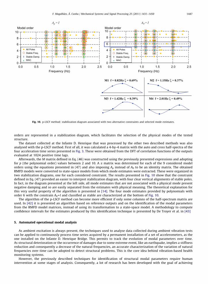
The dataset collected at the Infante D. Henrique that was processed by the other two described methods was alsoanalysed with the p-LSCF method. First of all, it was calculated a 4-by-4 matrix with the auto and cross half-spectra of thefour acceleration time series presented in Fig. 3. These were obtained from the DFT of correlation functions of the outputsevaluated at 1024 positive time lags.

Afterwards, the M matrix defined in Eq. (46) was constructed using the previously presented expressions and adoptingfor p (the polynomial order) values between 2 and 10. A a matrix was determined for each of the 9 considered modelorders using the equations presented in (47) and also imposing Ap instead of A0 to be an identity matrix. The obtainedRMFD models were converted to state-space models from which mode estimates were extracted. These were organized intwo stabilization diagrams, one for each considered constraint. The results presented in Fig. 10 show that the constraintdefined in Eq. (47) provided an easier to interpret stabilization diagram, with four clear vertical alignments of stable poles.In fact, in the diagram presented at the left side, all mode estimates that are not associated with a physical mode presentnegative damping and so are easily separated from the estimates with physical meaning. The theoretical explanation forthis very useful property of the algorithm is presented in [14]. The four mode estimates provided by polynomials withorder 6 with the constrain A0= I and classified as stable are characterized at the bottom of Fig. 10.

The algorithm of the p-LSCF method can become more efficient if only some columns of the half-spectrum matrix areused. In [42] it is presented an algorithm based on reference outputs and on the identification of the modal parametersfrom the RMFD model matrices, instead of using its transformation to a state-space model. A methodology to computeconfidence intervals for the estimates produced by this identification technique is presented by De Troyer et al. in [43]

5. Automated operational modal analysis

As ambient excitation is always present, the techniques used to analyse data collected during ambient vibration testscan be applied to continuously process time series acquired by a permanent installation of a set of accelerometers, as theone installed on the Infante D. Henrique Bridge. This permits to track the evolution of modal parameters over time.As structural deterioration or the occurrence of damages due to some extreme event, like an earthquake, implies a stiffnessreduction and consequently a decrease of the natural frequencies, an accurate characterization of the variation of naturalfrequencies over time can be adopted to detect structural problems. This is the core idea behind vibration-based healthmonitoring systems.

However, the previously described techniques for identification of structural modal parameters require humanintervention at some stages of analysis. Consequently, a lot of research has been developed with the goal of achieving


algorithms that can automatically extract accurate estimates of the structure modal parameters from its continuouslyrecorded responses during normal operation conditions.

In the context of the monitoring project carried out at the Infante D. Henrique Bridge, it was used an innovativemethodology for the automatic identification of modal parameters, using parametric identification methods, that is basedon a hierarchical clustering algorithm. The method is suitable for the analysis of data produced by any parametricidentification technique that provides estimates of natural frequencies, modal damping ratios and mode shapes for modelsof several orders. All the mode estimates provided by the identification algorithm are compared using a similarity measurethat depends on the natural frequencies and on the MAC (Eq. (27)) between mode shape estimates. It groups the modeestimates associated with the same physical mode and permits the separation of the numerical or noisy estimates. All thedetails of this algorithm and also a review of other available methodologies are presented in [44]. Fig. 11 shows the timeevolution of the modes analysed in the previous section (mode M1 to M4 characterized in Fig. 10). The estimates of thenatural frequencies presented in the graphics resulted from the automatic processing of all the datasets collected from13/09/2007 to 12/05/2010 with the cluster analysis applied to the outputs of the p-LSCF method. The influence of theannual temperature cycles on the natural frequencies is evident.

The processing of data collected by dynamic monitoring systems with the aim of identifying structural deficienciescomprehends not only automatic identification of modal parameters, but also elimination of the environmental andoperational effects on natural frequencies. As the identification of very small structural changes is aimed to permit thedetection of damages in an early phase of development, the minute effects of for instance the temperature or the trafficintensity over a bridge on the natural frequencies have to be minimized. Therefore, monitoring software based on OMA hasto include three components: (i) automatic identification of modal parameters, (ii) elimination of the environmental andoperational effects on modal parameters, (iii) calculation of an index able to flag relevant frequency shifts. These steps areillustrated in Fig. 12 using results from the Infante D. Henrique Bridge. The algorithm for automated operational modalanalysis, in continuous operation for more than 2 years, has permitted the characterization of the time evolution of thebridge first 12 natural frequencies. The algorithms implemented to calculate an index able to detect structural anomaliesprove to be efficient on identification of numerically simulated damages. All the details of this analysis are described in[45]. In [46], it is presented another application where the ability of a vibration-based monitoring systems to detectdamages was proven, in this case with the introduction of real damages in the bridge under study.

Fig. 11. Time evolution of the natural frequencies of the first four vertical bending modes.

Acceleration time series

time

Nat

ural

freq

uenc

ies

time

undamaged

(i)

(ii)

(iii)

damaged

Fig. 12. Main processing steps of a vibration-based health monitoring system.


6. Conclusions

This tutorial paper presents an introduction to the use of operational modal analysis. A brief review of the theoreticalbackground of alternative models of dynamic systems is followed by the description of three of the most powerfulalgorithms for the identification of modal parameters from structural responses to ambient excitation. In order to make theexposition more didactic, the most important mathematical steps were illustrated with the processing of data collected inan arch bridge. At the end, it was stressed the usefulness of operational modal analysis in the context of Structural HealthMonitoring systems.

Some of the most important references that permit a further broadening and deepening of the readers knowledge aboutthe theoretical aspects involved in operational modal analysis have already been mentioned in the introduction of Section4. Now, it is relevant to point out some works with recent and interesting applications. In [47], it is described the ambientvibration test of the Humber Bridge, the largest suspension bridge in the United Kingdom; Siringoringo and Fujino [48]describe the processing of a database collected in a suspension bridge in Japan (Hakucho Bridge); in [49] several relevantapplications on bridges and other special structures are presented; in [50], it is demonstrated the usefulness of ambientvibration tests in the context of the implementation of vibration control devices; Pakzad and Fences [51] present theresults obtained with an ambient vibration test performed on the Golden Gate Bridge with wireless sensors; Carne andJames III [52] describe the use of OMA in wind turbines testing; reference [53] characterizes the monitoring of historicalmasonry structures, taking profit from OMA.

The applications on large civil engineering structures described in the previously mentioned papers prove thatoperational modal analysis has already achieved significant maturity. However, there are also some limitations, such as theuncertainty of the modal damping estimates [54], which justify the need for further research to make this experimentaltool even more powerful and useful.

References

[1] D.J. Ewins, Modal Testing: Theory and Practice, Research Studies Press, UK, 2000.[2] W. Heylen, S. Lammens, P. Sas, Modal Analysis Theory and Testing, KULeuven, Belgium, 2007.[3] N. Maia, J. Silva, Theoretical and Experimental Modal Analysis, Research Studies Press Ltd., 1997.[4] A. Cunha, E. Caetano, Experimental modal analysis of civil engineering structures, Sound and Vibration 6 (40) (2006) 12–20.[5] E. Parloo, P. Verboven, P. Guillaume, M.V. Overmeire, Sensitivity-based operational mode shape normalization, Mechanical Systems and Signal

Processing 16 (5) (2002) 757–767.[6] R. Brincker, P.H. Kirkegaard, Special issue on operational modal analysis, Mechanical Systems and Signal Processing 24 (5) (2009) 1209–1212.[7] A. Ad~ao da Fonseca, F. Millanes Mato, Infante Henrique Bridge over the River Douro, Porto, Portugal, Structural Engineering International 15 (2)

(2005) 85–87.[8] F. Magalh~aes, A. Cunha, E. Caetano, Dynamic monitoring of a long span arch bridge, Engineering Structures 30 (11) (2008) 3034–3044.[9] M.I. Friswell, J.E. Mottershead, Finite Element Model Updating in Structural Dynamics, Kluwer Academic Publishers, 1995.

[10] J.-N. Juang, Applied System Identification, Prentice Hall, Englewood Cliffs, NJ, USA, 1994.[11] B. Peeters, System identification and damage detection in civil engineering, Ph.D. Thesis, Katholieke Universiteit, Leuven, Belgium, 2000.[12] P. Van Overschee, B. De Moor, Subspace Identification for Linear Systems, Kluwer Academic Publishers, Leuven, Belgium, 1996.[13] B. Cauberghe, Applied frequency-domain system identification in the field of experimental and operational modal analysis, Ph.D. Thesis, Vrije

Universiteit, Brussel, Belgium, 2004.[14] E. Reynders, System identification and modal analysis in structural mechanics, Ph.D. Thesis, Katholieke Universiteit, Leuven, Belgium, 2009.[15] L. Ljung, System Identification: Theory for the User, Prentice-Hall, New Jersey, 1999.[16] V.R. MacLamore, G.C. Hart, I.R. Stubbs, Ambient vibration of two suspension bridges, Journal of the Structural Division, ASCE 97 (ST10) (1971)

2567–2582.[17] P., Guillaume, L. Hermans, H. Van der Auweraer, Maximum likelihood identification of modal parameters from operational data, in: Proceedings of

IMAC 17, International Modal Analysis Conference, Kissimmee, FL, USA, 1999.[18] C. Devriendt, P. Guillaume, The use of transmissibility measurements in output-only modal analysis, Mechanical Systems and Signal Processing 21

(7) (2007) 2689–2696.[19] J. Bendat, A. Piersol, Engineering Applications of Correlation and Spectral Analysis, John Wiley & Sons, USA, 1980.[20] J.-N. Juang, R.S. Pappa, An eigensystem realization algorithm for modal parameter identification and model reduction, Journal of Guidance, Control,

and Dynamics 8 (5) (1985) 620–627.[21] G.H. James, T.G. Carne, J.P. Lauffer, A.R. Nard, Modal testing using natural excitation, in: Proceedings of IMAC 10, International Modal Analysis

Conference, San Diego, USA, 1992.[22] P. Andersen, Identification of civil engineering structures using vector ARMA models, Ph.D. Thesis, Aalborg University, Denmark, 1997.[23] A.V. Oppenheim, R.W. Schafer, Digital Signal Processing, Prentice-Hall, 1975.[24] P.D. Welch, The use of fast Fourier transform for the estimation of power spectra: a method based on time averaging over short modified

periodograms, IEEE Transaction on Audio and Electro-Acoustics AU-15 (1967) 2.[25] R. Brincker, L. Zhang, P. Andersen, Modal identification from ambient responses using frequency domain decomposition, in Proceedings of the IMAC

18, International Modal Analysis Conference, San Antonio, USA, 2000.[26] M. Prevosto, Algorithmes D’Identification des Caracteristiques Vibratoires de Structures Mecaniques Complexes, Ph.D. Thesis, Universite de Rennes I,

France, 1982.[27] M.R. Correa, A.C. Costa, Dinamic tests of the bridge over the Arade River, in: J.A. Fernandes, L.O. Santos (Eds.), Cable-stayed Bridges of Guadiana and

Arade, Book, LNEC, 1992 (in Portuguese).[28] C.Y. Shih, Y.G. Tsuei, R.J. Allemang, D.L. Brown, Complex mode indicator function and its application to spatial domain parameter estimation,

Mechanical Systems and Signal Processing 2 (4) (1988) 367–377.[29] R.J. Allemang, D.L. Brown, A correlation coefficient for modal vector analysis, in: Proceedings of the IMAC 1, International Modal Analysis Conference,

Orlando, FL, USA, 1982.[30] R.W. Clough, J. Penzien, Dynamics of Structures, McGraw-Hill, 1993.[31] R., Brincker, C. Ventura, P. Andersen, Damping estimation by frequency domain decomposition, in Proceedings of the IMAC 19, International Modal

Analysis Conference, Kissimmee, FL, USA, 2001.


[32] N.-J. Jacobsen, P. Andersen, R. Brincker, Applications of frequency domain curve-fitting in the EFDD technique, in: Proceedings of IMAC 26,International Modal Analysis Conference, Orlando, FL, USA, 2008.

[33] F. Magalh~aes, E. Caetano, A. Cunha, Operational modal analysis and finite element model correlation of the Braga Stadium suspended roof,Engineering Structures 30 (6) (2008) 1688–1698.

[34] J. Rodrigues, R. Brincker, P. Andersen, Improvement of frequency domain output-only modal identification from the application of the randomdecrement technique, in: Proceedings of the IMAC 22, International Modal Analysis Conference, Dearborn, USA, 2004.

[35] L. Zhang, T. Wang, Y. Tamura, A frequency-spatial domain decomposition (FSDD) method for operational modal analysis, Mechanical Systems andSignal Processing 24 (5) (2009) 1227–1239.

[36] S.Y. Kung, A new identification and model reduction algorithm via singular value decomposition, in Proceedings of the 12th Asilomar Conference onCircuits, Systems and Computers, USA, 1978.

[37] MatLab2000, Using MATLAB Version 6, The MathWorks.[38] B. Peeters, G. De Roeck, Reference-based stochastic subspace identification for output-only modal analysis, Mechanical Systems and Signal

Processing 13 (6) (1999) 855–878.[39] E. Reynders, R. Pintelon, G. De Roeck, Uncertainty bounds on modal parameters obtained from stochastic subspace identification, Mechanical

Systems and Signal Processing 22 (4) (2008) 948–969.[40] P. Guillaume, P. Verboven, S. Vanlanduit, H. Van der Auweraer, B. Peeters, A poly-reference implementation of the least-squares complex frequency-

domain estimator, in: Proceedings of the IMAC 21, International Modal Analysis Conference, Kissimmee, FL, USA, 2003.[41] B. Peeters, H. Van Der Auweraer, P. Guillaume, J. Leuridan, The PolyMAX frequency-domain method: a new standard for modal parameters

estimation?, Shock and Vibration 11 (2004) 395–409.[42] B. Peeters, H. Van Der Auweraer, PolyMax: a revolution in operational modal analysis, in: Proceedings of the IOMAC, International Operational Modal

Analysis Conference, Copenhagen, Denmark, 2005.[43] T. De Troyer, P. Guillaume, R. Pintelon, S. Vanlanduit, Fast calculation of confidence intervals on parameter estimates of least-squares frequency-

domain estimators, Mechanical Systems and Signal Processing 23 (2) (2009) 261–273.[44] F. Magalh~aes, A. Cunha, E. Caetano, Online automatic identification of the modal parameters of a long span arch bridge, Mechanical Systems and

Signal Processing 23 (2) (2009) 316–329.[45] F. Magalh~aes, Operational modal analysis for testing and monitoring of bridges and special structures, Ph.D. Thesis, Faculty of Engineering of the

University of Porto, 2010.[46] B. Peeters, G. De Roeck, One-year monitoring of the Z24-Bridge: environmental effects versus damage events, Earthquake Engineering and Structural

Dynamics 30 (2) (2001) 149–171.[47] J.M.W. Brownjohn, F. Magalh~aes, E. Caetano, A. Cunha, Ambient vibration re-testing and operational modal analysis of the Humber Bridge,

Engineering Structures (2010).[48] D.M. Siringoringo, Y. Fujino, System identification of a suspension bridge from ambient vibration response, Engineering Structures 30 (2) (2008)

462–477.[49] A. Cunha, E. Caetano, F. Magalh~aes, Output-only dynamic testing of bridges and special structures, Structural Concrete (Fib) 8 (2) (2007) 67–85.[50] E. Caetano, A. Cunha, F. Magalh~aes, C. Moutinho, Studies for controlling human-induced vibration of the Pedro e Ines footbridge, Portugal. Part 1:

Assessment of dynamic behaviour, Engineering Structures 32 (4) (2010) 1069–1081.[51] S.N. Pakzad, G.L. Fences, Statistical analysis of vibration modes of a suspension bridge using spatially dense wireless sensor network, Journal of

Structural Engineering 135 (7) (2009) 863–872.[52] T.G. Carne, G.H. James III, The inception of OMA in the development of modal testing technology for wind turbines, Mechanical Systems and Signal

Processing 24 (5) (2009) 1213–1226.[53] L.F. Ramos, L. Marques, P.B. Lorenc-o, Guido De Roeck, A. Campos Costa, J. Roque, Monitoring historical masonry structures with operational modal

analysis: two case studies, Mechanical Systems and Signal Processing 24 (5) (2009) 1291–1305.[54] F. Magalh~aes, A. Cunha, E. Caetano, R. Brincker, Damping estimation using free decays and ambient vibration tests, Mechanical Systems and Signal

Processing 24 (5) (2009) 1274–1290.

Explaining operational modal analysis with data from an arch bridge

Documents

Transcript of Explaining operational modal analysis with data from an arch bridge