Explaining heterogeneity - Cochrane Methods...= 4.04 • Two subgroups, so 2 –1 = 1 degree of...
69
Explaining heterogeneity Julian Higgins School of Social and Community Medicine, University of Bristol, UK
Transcript of Explaining heterogeneity - Cochrane Methods...= 4.04 • Two subgroups, so 2 –1 = 1 degree of...

Explaining heterogeneity
Julian Higgins
School of Social and Community Medicine, University of Bristol, UK

Outline
1. Revision and remarks on fixed-effect and random-effects meta-analysis methods (and interpretation under heterogeneity)
Explaining heterogeneity:
2. Subgroup analysis
3. Meta-regression
4. Problems
5. Closing remarks
• Example 1: Trials of exercise for treatment of depression

Part 1: Revision and remarks on fixed-effect and random-effects meta-analysis methods
3
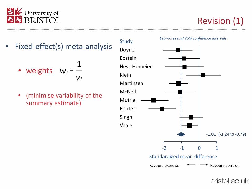
Revision (1)
• Fixed-effect(s) meta-analysis
• weights
• (minimise variability of the summary estimate)
-2 -1 0 1
Study
Mutrie
McNeil
Reuter
Doyne
Hess-Homeier
Epstein
Martinsen
Singh
Klein
Veale
Favours exercise
Standardized mean difference
Favours control
Estimates and 95% confidence intervals
-1.01 (-1.24 to -0.79)
1i
i
=wv
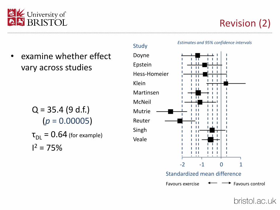
Revision (2)
• examine whether effect vary across studies
Q = 35.4 (9 d.f.)(p = 0.00005)
τDL = 0.64 (for example)
I2 = 75%
-2 -1 0 1
Study
Mutrie
McNeil
Reuter
Doyne
Hess-Homeier
Epstein
Martinsen
Singh
Klein
Veale
Favours exercise
Standardized mean difference
Favours control
Estimates and 95% confidence intervals
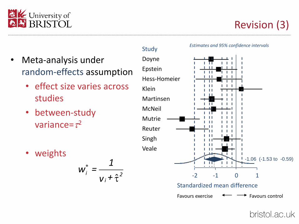
Revision (3)
• Meta-analysis under random-effects assumption
• effect size varies across studies
• between-study variance=2
• weights
-2 -1 0 1
Study
Mutrie
McNeil
Reuter
Doyne
Hess-Homeier
Epstein
Martinsen
Singh
Klein
Veale
Favours exercise
Standardized mean difference
Favours control
Estimates and 95% confidence intervals
-1.06 (-1.53 to -0.59)
i 2
i
1w =
+v
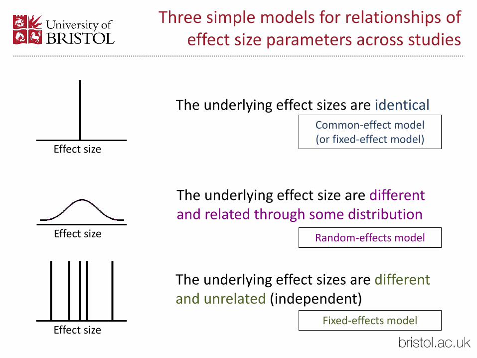
Three simple models for relationships of effect size parameters across studies
Effect size
The underlying effect sizes are identical
Effect size
The underlying effect sizes are different and unrelated (independent)
Common-effect model (or fixed-effect model)
Random-effects model
Fixed-effects model
Effect size
The underlying effect size are different and related through some distribution
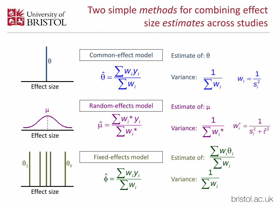
Two simple methods for combining effect size estimates across studies
Effect size
θ
μ
Effect size
Effect size
θ1 θk
2 2
1
ˆi
i
ws
*ˆ
*
i i
i
w y
w 1
*iw
Random-effects model Estimate of: μ
Variance:
ˆ i i
i
w y
w
i i
i
w
w
1
iw
Fixed-effects model Estimate of:
Variance:
ˆ i i
i
w y
w 1
iw
Common-effect model Estimate of: θ
Variance: 2
1i
i
ws

Three simple models for relationships of effect size parameters across studies
Effect size
Effect size
Common-effect model (or fixed-effect model)
Fixed-effects model
Complication is that the fixed-effect meta-analysis method can be
interpreted under either of these models

Aside: an interpretation of the weighted average under fixed-effects model
• A weighted average of the study-specific effects seen in the individual study populations, where the weight for study population i is proportional to both the number of participants selected (pi) and to how much information is contributed per subject (ri)
• No assumption of homogeneity is required
• But heterogeneity is ignored in the analysis so inference on this is required
• this inference is statistically independent
• The empirical weights are poor estimates of piri unless the studies are large
i i i
i i
p r
p r
Rice, Higgins and Lumley (submitted)
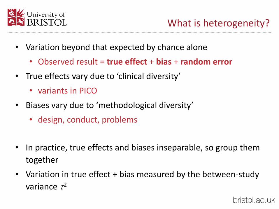
• Variation beyond that expected by chance alone
• Observed result = true effect + bias + random error
• True effects vary due to ‘clinical diversity’
• variants in PICO
• Biases vary due to ‘methodological diversity’
• design, conduct, problems
• In practice, true effects and biases inseparable, so group them
together
• Variation in true effect + bias measured by the between-study
variance 2
What is heterogeneity?

Exploring heterogeneity
In which types of trials does the intervention work best?
• Characteristics of studies may be associated with the size of treatment effect
• Does the intervention work better if given for longer?
• Are smaller odds ratios observed in high-risk populations?
• Is there a relationship between sample size and effect size (e.g. due to publication bias)?
• Is inadequate allocation concealment associated with a larger effect estimate?
• Is A better than B, when they’ve each only been compared with C? For discrete characteristics, can use subgroup analyses
• We can use subgroup analyses or meta-regression to answer questions like these

Subgroup analysis
• Divide up the studies
• e.g. by duration of trial
• Test for subgroup differences:
• can apply Q test to subgroup results
• here, P = 0.28MutrieMcNeil
Doyne
Hess-Homeier
Epstein
4-8 weeks follow-up
-1.33 (-1.99 to -0.67)
-2 -1 0 1
Reuter
Martinsen
Singh
Klein
Veale
Favours exercise
Standardized mean difference
Favours control
Estimates and 95% confidence intervals
> 8 weeks follow-up
-0.82 (-1.46 to -0.19)

Meta-regression
• Examine heterogeneity
• Predict effect according to length of follow-up
• Difference in SMDs = 0.18 (95% CI 0.02 to 0.34): i.e. SMD decreases by 0.2 for each extra week of follow up -2 -1 0 1
Mutrie
McNeil
Reuter
DoyneHess-HomeierEpstein
Martinsen
Singh
KleinVeale
Favours exercise
Standardized mean difference
Favours control
Estimates and 95% confidence intervals
4
12
8
10
6
Follow-up
Part 2: Subgroup analysis
15

Subgroup analyses
• Split data into subgroups:
• Subsets of patients
• Subsets of studies
• Do separate meta-analyses for each
• Subgroup analyses done for three reasons
• To answer multiple questions (one for each subset of studies)
• To examine whether the effect is different in different subgroups (comparing subgroups)
• To assess whether restricting analysis to one subgroup changes the conclusion (sensitivity analysis)

Subgroup analyses
Behavioural interventions for smokeless tobacco use cessation
Abstinence from all tobacco use (where reported) at 6 months or more

Subgroup analyses

Comparing two subgroups
• Simple statistics: take the difference in point estimates and add their variances
• all on the log scale for ratio measures
19
Subgroup OR OR_CI_low OR_CI_upp lnOR lnOR_CI_low lnOR_CI_upp lnOR_var
Randomisation by organisation
1.36 1.12 1.64 0.307 0.113 0.495 0.009
Individual randomisation
1.76 1.49 2.07 0.565 0.399 0.728 0.007
RATIO DIFF SUMComparison of subgroups
0.773 0.601 0.994 -0.258 -0.510 -0.006 0.016
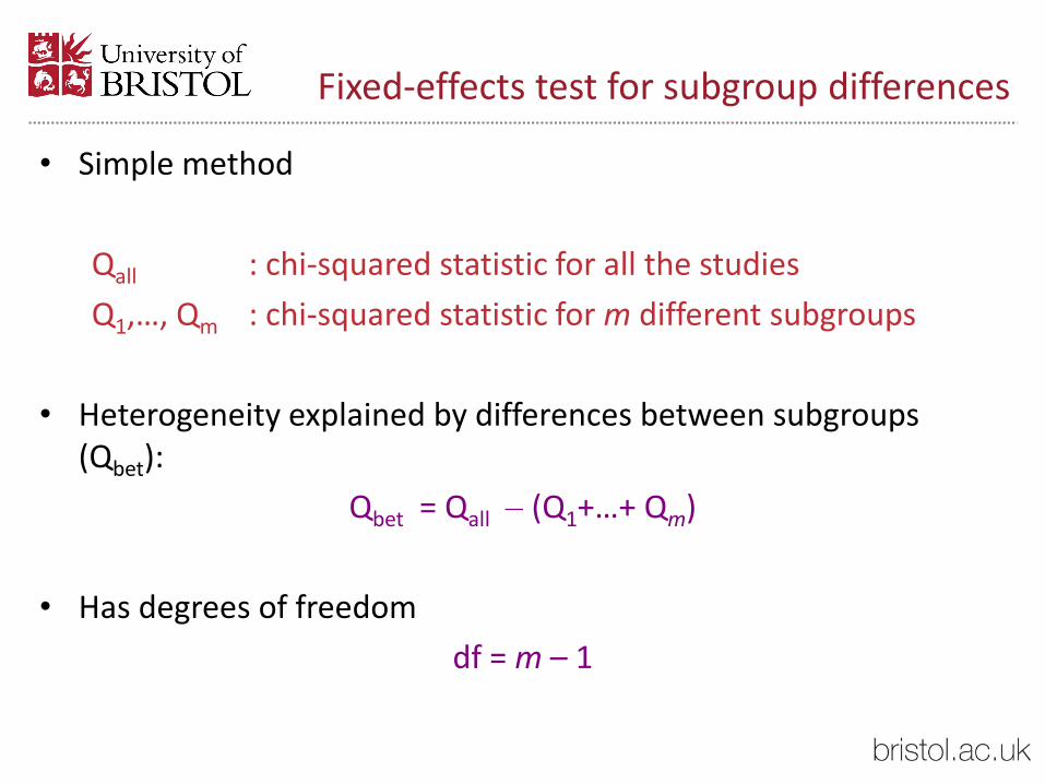
Fixed-effects test for subgroup differences
• Simple method
Qall : chi-squared statistic for all the studies
Q1,…, Qm : chi-squared statistic for m different subgroups
• Heterogeneity explained by differences between subgroups (Qbet):
Qbet = Qall – (Q1+…+ Qm)
• Has degrees of freedom
df = m – 1

Fixed-effects test for subgroup differences
Qall
Q2
Q1

Fixed-effects test for subgroup differences
Qbet = 34.42 – (24.38 + 6.00)
= 4.04
• Two subgroups, so 2 – 1 = 1 degree of freedom
• Chi-squared value of 4.04 with 1 degree of freedom: P = 0.044
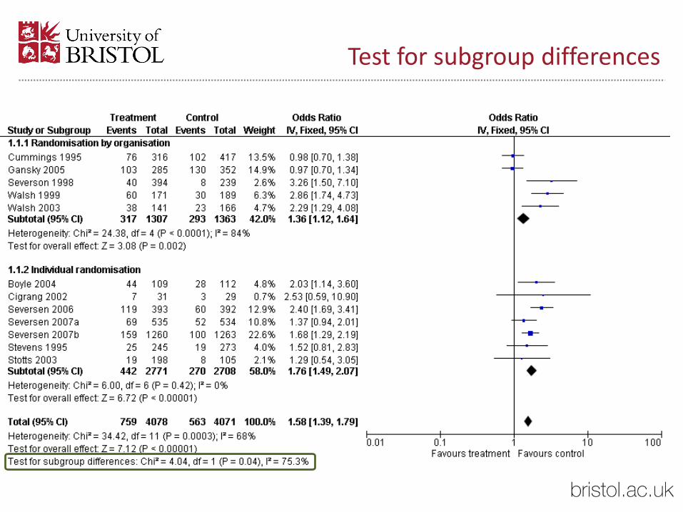
Test for subgroup differences

General test for subgroup differences
• Just do a test for heterogeneity across the results of all the subgroups
• Fine for any number of subgroups, and any type of analysis within the subgroups
“Study 1”
“Study 2”

Part 3: Meta-regression
26

Meta-regression
• A general framework for looking at possible explanations for differences in effect sizes across studies
• A test for subgroup differences can be done using meta-regression
• But meta-regression also good for continuous characteristics
• Linear regression
• outcome variable = effect size (e.g. SMD or logRR)
• explanatory variable = summary description of study (e.g. duration or location)
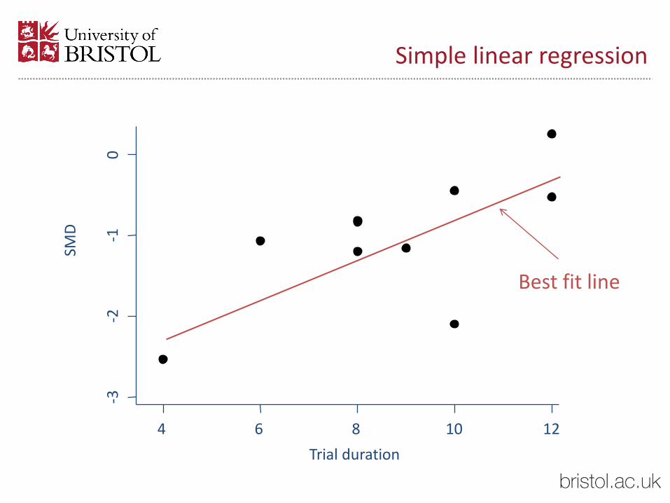
Simple linear regression
Best fit line
-3-2
-10
4 6 8 10 12
SMD
Trial duration

Why we don’t use simple linear regression
• Just as in meta-analysis, the studies are different sizes, and should have different influences on the analysis
• There’s a difference between
-3-2
-10
4 6 8 10 12Trial duration
SMD
and
-3-2
-10
4 6 8 10 12Trial duration
SMD big study small study

-1-.
50
.51
Pre
ve
nte
d fra
ctio
n
1960 1970 1980 1990 2000
Year
Has effectiveness of fluoride gels changed over time? Marinho et al (2004)
‘Bubble plot’:
Circles proportional to inverse-variance
(weight in a meta-analysis)

Number of sessions of CBT
-2-1
.5-1
-.5
0.5
SM
D
5 10 15 20 25 30
Number of Sessions

Fixed-effect meta-analysis
Treatmenteffect
Effect estimate
Random error
Common treatment effect
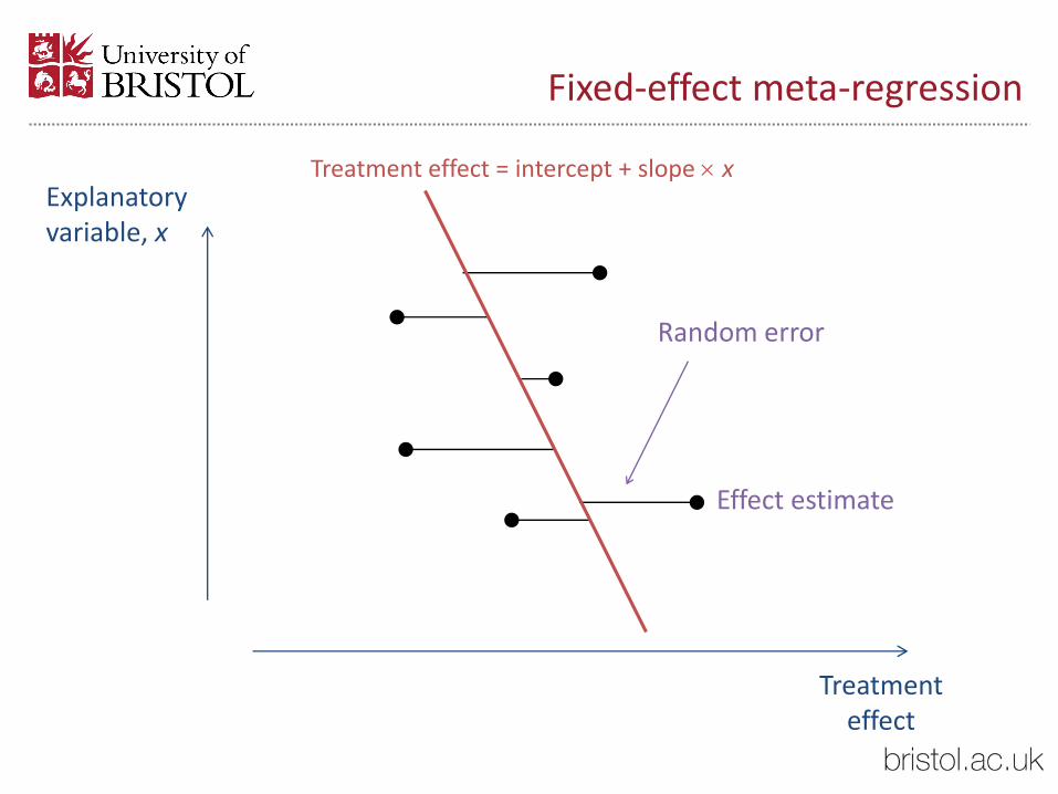
Fixed-effect meta-regression
Treatmenteffect
Effect estimate
Random error
Explanatory variable, x
Treatment effect = intercept + slope x

The other way round (the convention for plotting)
Explanatory variable, x
Treatmenteffect
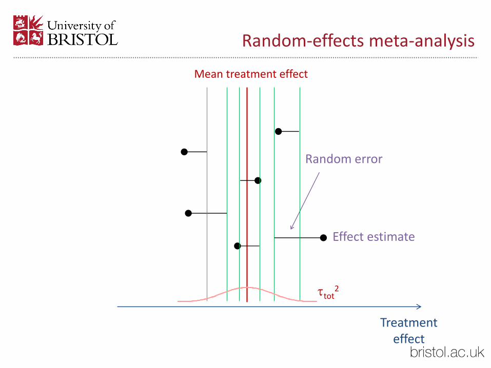
Random-effects meta-analysis
Treatmenteffect
Effect estimate
Random error
tot2
Mean treatment effect
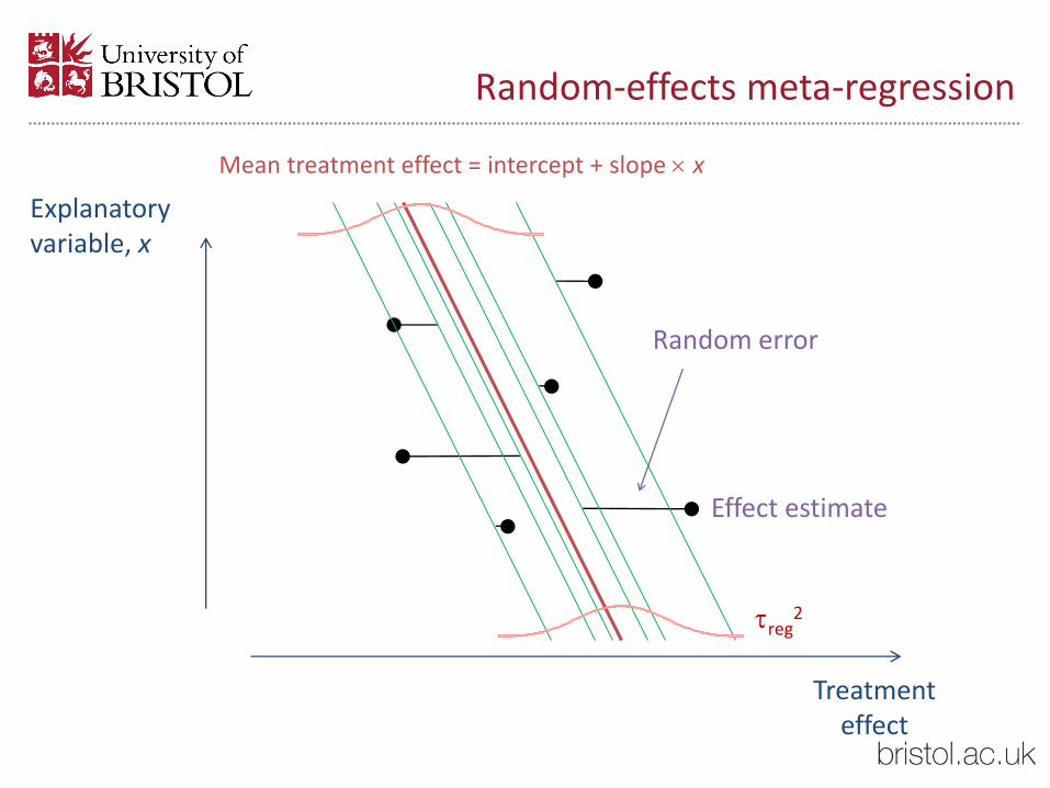
Random-effects meta-regression
Explanatory variable, x
Treatmenteffect
Mean treatment effect = intercept + slope x
Random error
reg2
Effect estimate

Proportion of heterogeneity explained
• Compare
heterogeneity variance from random-effects meta-analysis ( )
with
heterogeneity variance from random-effects meta-regression ( )
• % variance explained =
• A useful measure of the explanatory ability of a (set of) covariate(s)
2 2
2100% tot reg
tot
2tot
2reg

Example - BCG vaccination
It has been recognised for many years that the protection given by BCG against tuberculosis varied between trials
Risk ratios:
MRC trial (UK) 0.24 (95% CI 0.18 to 0.31)
Madras, (South India) 1.01 (95% CI 0.89 to 1.14)
Random-effects meta-analysis (Colditz et al. 1994)
Summary (random effects) RR: 0.49 (95% CI 0.34 to 0.70)
“the results of this meta-analysis lend added weight and confidence to arguments favouring the use of BCG vaccine”

NOTE: Weights are from random effects analysis
. (0.14, 1.77)with estimated predictive interval
Overall (I-squared = 92.1%, p = 0.000)
4
2
11
1
9
8
ID
13
7
6
5
10
3
12
Study
0.49 (0.34, 0.70)
0.24 (0.18, 0.31)
0.20 (0.09, 0.49)
0.71 (0.57, 0.89)
0.41 (0.13, 1.26)
0.63 (0.39, 1.00)
1.01 (0.89, 1.14)
RR (95% CI)
0.98 (0.58, 1.66)
0.20 (0.08, 0.50)
0.46 (0.39, 0.54)
0.80 (0.52, 1.25)
0.25 (0.15, 0.43)
0.26 (0.07, 0.92)
1.56 (0.37, 6.53)
0.49 (0.34, 0.70)
0.24 (0.18, 0.31)
0.20 (0.09, 0.49)
0.71 (0.57, 0.89)
0.41 (0.13, 1.26)
0.63 (0.39, 1.00)
1.01 (0.89, 1.14)
RR (95% CI)
0.98 (0.58, 1.66)
0.20 (0.08, 0.50)
0.46 (0.39, 0.54)
0.80 (0.52, 1.25)
0.25 (0.15, 0.43)
0.26 (0.07, 0.92)
1.56 (0.37, 6.53)
Favours vaccination Favours no vaccination
1.1 .2 .5 1 2 5 10
Risk ratio
BCG vaccination to prevent tuberculosis

NOTE: Weights are from random effects analysis
. (0.14, 1.77)with estimated predictive interval
Overall (I-squared = 92.1%, p = 0.000)
11
5
1
8
7
9
10
2
4
6
13
3
ID
12
Study
0.49 (0.34, 0.70)
0.41 (0.13, 1.26)
0.63 (0.39, 1.00)
1.01 (0.89, 1.14)
0.25 (0.15, 0.43)
1.56 (0.37, 6.53)
0.26 (0.07, 0.92)
0.46 (0.39, 0.54)
0.80 (0.52, 1.25)
0.20 (0.08, 0.50)
0.98 (0.58, 1.66)
0.20 (0.09, 0.49)
0.71 (0.57, 0.89)
RR (95% CI)
0.24 (0.18, 0.31)
44
27
13
42
33
42
44
13
19
33
55
18
latitude
52
Absolute
Favours vaccination Favours no vaccination
1.1 .2 .5 1 2 5 10
Risk ratio
BCG vaccination to prevent tuberculosis
Berkey et al, 1995

Meta-regression: Dependence of BCG vaccine efficacy on study latitude
2 (m-a) = 0.313 2 (m-reg) = 0.076
so 76% of variance is explained
.51
1.5
10 20 30 40 50 60
Latitude
Ris
k ra
tio

Hartung-Knapp
• Simulation study:
“Of the different methods evaluated, only the Knapp and Hartungmethod and the permutation test provide adequate control of the Type I error rate across all conditions. Due to its computational simplicity, the Knapp and Hartung method is recommended as a suitable option for most meta-analyses.”
Viechtbauer et al 2015
• More on permutation tests later
42

Variance explained
Within studies:
8%
Between studies (I2):92%
Unexplained: 24%
Explained by latitude (R2):76%
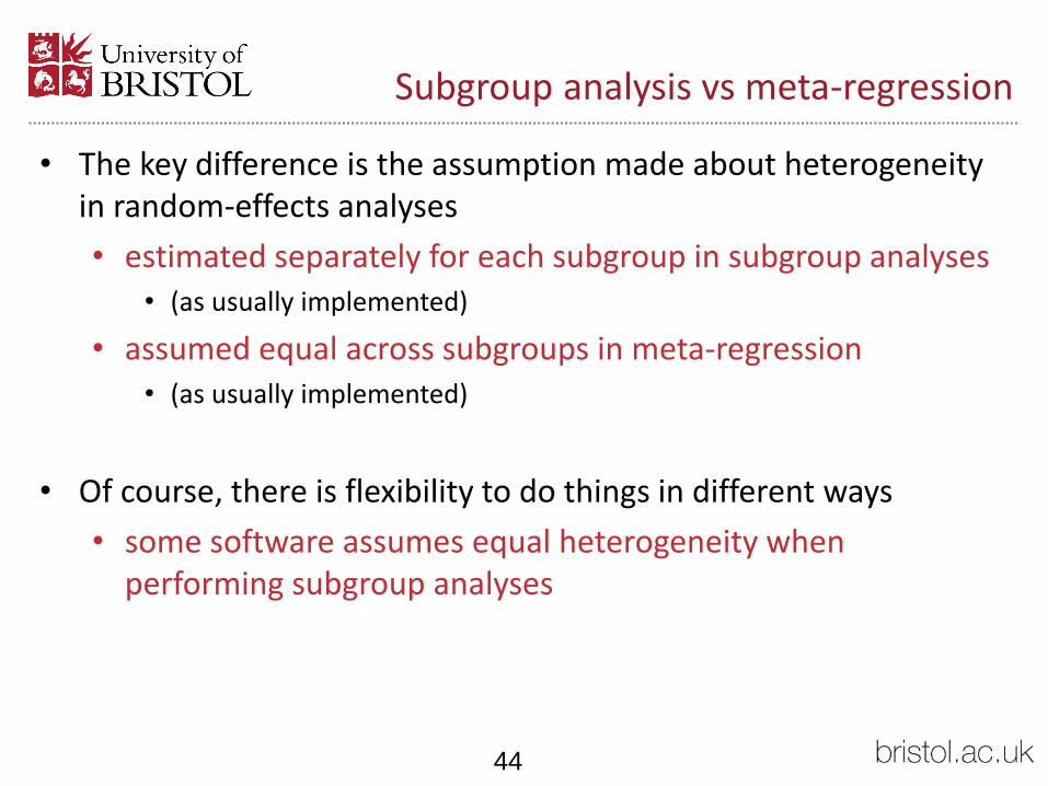
Subgroup analysis vs meta-regression
• The key difference is the assumption made about heterogeneity in random-effects analyses
• estimated separately for each subgroup in subgroup analyses • (as usually implemented)
• assumed equal across subgroups in meta-regression • (as usually implemented)
• Of course, there is flexibility to do things in different ways
• some software assumes equal heterogeneity when performing subgroup analyses
44
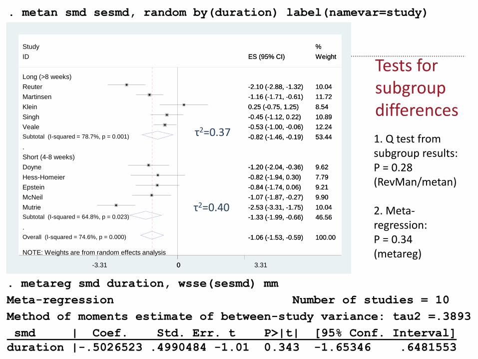
NOTE: Weights are from random effects analysis
.
.
Overall (I-squared = 74.6%, p = 0.000)
Doyne
McNeil
Singh
Short (4-8 weeks)
Subtotal (I-squared = 64.8%, p = 0.023)
Martinsen
Subtotal (I-squared = 78.7%, p = 0.001)
Klein
Epstein
Mutrie
Veale
ID
Hess-Homeier
Reuter
Study
Long (>8 weeks)
-1.06 (-1.53, -0.59)
-1.20 (-2.04, -0.36)
-1.07 (-1.87, -0.27)
-0.45 (-1.12, 0.22)
-1.33 (-1.99, -0.66)
-1.16 (-1.71, -0.61)
-0.82 (-1.46, -0.19)
0.25 (-0.75, 1.25)
-0.84 (-1.74, 0.06)
-2.53 (-3.31, -1.75)
-0.53 (-1.00, -0.06)
ES (95% CI)
-0.82 (-1.94, 0.30)
-2.10 (-2.88, -1.32)
100.00
9.62
9.90
10.89
46.56
11.72
53.44
8.54
9.21
10.04
12.24
Weight
7.79
10.04
%
0-3.31 0 3.31
. metan smd sesmd, random by(duration) label(namevar=study)
. metareg smd duration, wsse(sesmd) mm
Meta-regression Number of studies = 10
Method of moments estimate of between-study variance: tau2 =.3893
smd | Coef. Std. Err. t P>|t| [95% Conf. Interval]
duration |-.5026523 .4990484 -1.01 0.343 -1.65346 .6481553
τ2=0.37
τ2=0.40
1. Q test from subgroup results: P = 0.28 (RevMan/metan)
2. Meta-regression: P = 0.34(metareg)
Tests for subgroup differences

Interpretation of meta-regression coefficients
Continuous outcome (MD/SMD)
Dichotomous outcome (OR/RR)
Continuous explanatory variable
Difference in mean differences or in SMDs associated with 1 point increase in covariate
Ratio of ORs or of RRs associated with 1 point increase in covariate
Dichotomousexplanatory variable
Difference in mean differences or in SMDs between 2 groups
Ratio of ORs or of RRs between 2 groups
Meta-regression with dichotomous variable gives formal comparison between subgroups

Part 4: Problems
47

Problems with exploration of heterogeneity
• Observational relationships
• Confounding (correlation between characteristics)
• Aggregation bias
• Low power with few studies: false-negative findings
• Multiple characteristics: false-positive findings
Treatment effect Year of randomization Quality
Confounder
(associated with treatment effect and
year)
Thompson & Higgins (2002)

Aggregation bias
• Beware study characteristics that summarize participants within a study, e.g.
• average age
• % females
• average duration of follow-up
• % drop out

Relationship between treatment effect and average age
SMD
Average age in each study30 40 50 60 70
.01
.1
.5
1
2
10

Relationship between treatment effect and average age
SMD
Average age in each study30 40 50 60 70
.01
.1
.5
1
2
10

Aggregation bias
• Beware study characteristics that summarize participants within a study, e.g.
• average age
• % females
• average duration of follow-up
• % drop out
• Relationships across studies may not reflect relationships withinstudies
• The relationship between treatment effect and age, sex, etc is best measured within a study
• Needs individual participant data

Lack of power
• Unfortunately most meta-analyses in Cochrane reviews do not have many studies
• Meta-regression typically has low power to detect relationships
• Model diagnostics / adequacy difficult to assess

Selecting explanatory variables
• There are typically many, many explanatory variables to choose
from
• Heterogeneity can always be explained if you look at enough
of them
• Great risk of spurious findings

False-positive findings
• To guard against false-positives, meta-analysts are advised to
• Pre-specify characteristics in a protocol
• Limit to a small number
• Have a scientific rationale
• Beware ‘prognostic factors’
• Variables that predict clinical outcome don’t necessarily affect
treatment effects
• e.g. age may be strongly prognostic, but risk ratios may well be the
same irrespective of age

Ave. age
8 wks
16 wks
24 wks
Risk of false-positive findings
• Depends on
• number of studies
• extent of heterogeneity
• precision of effect estimates
1 2
Risk ratio
0.5
Risk ratio
1 20.5

5%
0 50% 83%
Sign
ific
ance
leve
l
Extent of inconsistency (I2)
25
%1
5%
0%
20
%1
0%
Fixed effect
Random effects
Example results: 10 studies, typical study weights, 1 covariate
Simulation study of false-positive rates

Solution? A permutation test
• But 1/3 of possible permutations give a relationship at least as strong as this
• So ‘real’ p = 0.33
Risk ratio
1 20.5
Duration
8 wks
16 wks
25 wks
P < 0.0001

18443355425213334419132742
33275242441819133344554213
18443355425213334419132742
55444213335242184419133327
StudyAbsolutelatitude
18443355425213334419132742
123456789
10111213
T(1000)T(1)
1000 times...
Shuffle1
Shuffle 1000
Meta-regression test statistic Tobs
Illustration

Permutation test p-value
• Compare with the values , … ,
• Count the number of ’s that exceed
• e.g. for BCG example = 2.44 ( = slope/SE);
• 54/1000 ’s exceed : p = 0.054
• c.f.
• FE: p < 10–10
• RE (standard normal): p = 0.012
T(1)Tobs T(1000)
Tobs
Tobs
T
TobsT
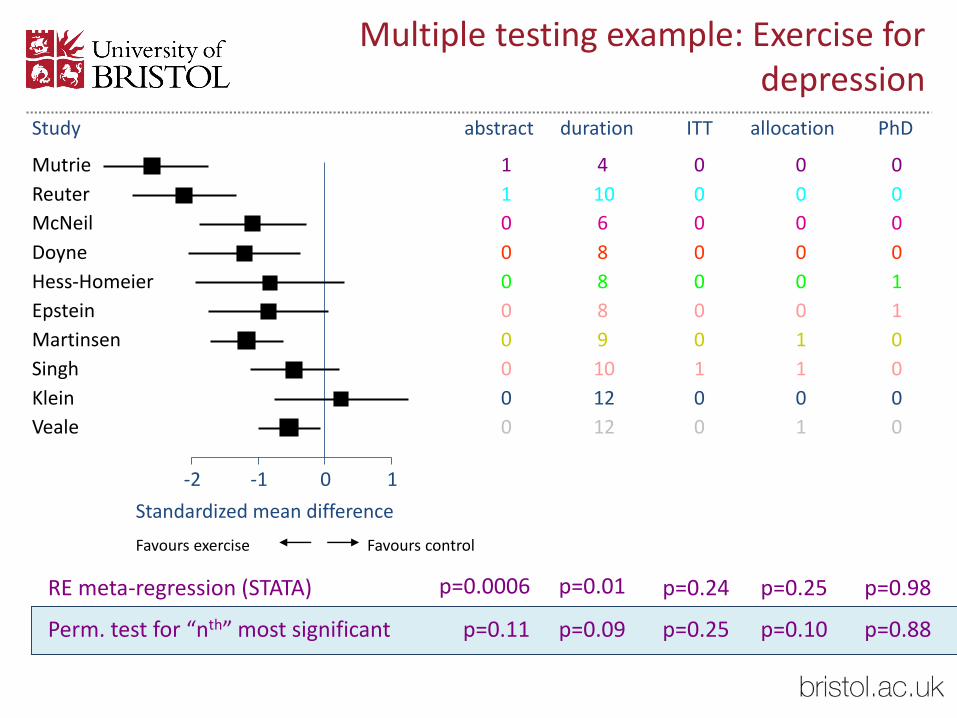
p=0.0006 p=0.01 p=0.24 p=0.25 p=0.98RE meta-regression (STATA)
p=0.11 p=0.09 p=0.25 p=0.10 p=0.88Perm. test for “nth” most significant
Multiple testing example: Exercise for depression
-2 -1 0 1
Study abstract duration ITT allocation PhD
Mutrie 1 4 0 0 0
McNeil 0 6 0 0 0
Reuter 1 10 0 0 0
Doyne 0 8 0 0 0
Hess-Homeier 0 8 0 0 1
Epstein 0 8 0 0 1
Martinsen 0 9 0 1 0
Singh 0 10 1 1 0
Klein 0 12 0 0 0
Veale 0 12 0 1 0
Favours exercise
Standardized mean difference
Favours control

Part 5: Closing remarksSelecting explanatory variables
Meta-regression in Cochrane reviews
Extensions
Summary
62

Selecting explanatory variables
• Specify a small number of characteristics in advance
• Ensure there is scientific rationale for investigating each characteristic
• effect modifier or prognostic factor?
• Make sure the effect of a characteristic can be identified
• does it differentiate studies?
• aggregation bias
• Think about whether the characteristic is closely related to another characteristic
• confounding

How many studies / characteristics?
• Typical guidance is to have 10 studies for each characteristic examined
• Some say 5 studies is enough

Including meta-regression in a Cochrane review
• Authors are encouraged to use meta-regression if appropriate
• ‘Bubble’ plots may be included as an ‘Other figure’
• Results should be presented in an ‘Additional table’
• Consider presenting something like:
Explanatory variable
Slope or Exp(slope)
95% confidence interval
Proportion of variation explained
Interpretation
Duration OR = 1.3 0.9 to 1.8 14% Odds ratio increases with duration(not statistically significant)

Extensions
• Baseline risk of the studied population (as measured in the control group) might be considered as an explanatory variable
• Beware! It is inherently correlated with treatment effects
• Special methods are needed (see Thompson et al 1997)
• Precision of the estimate (e.g. its standard error) might be considered as an explanatory variable to look at small study effects (may be suggestive of publication bias)
• Beware! It is often inherently correlated with treatment effects
• Special methods are needed (see Sterne et al 2011)
Key messages
• Subgroup analysis and meta-regression examine the relationship between treatment effects and one or more study-level characteristics
• Meta-regression is like usual linear regression, but
• study weights incorporated
• variation not explained by the characteristics should be accounted for
• random effects meta-regression does this;fixed effect meta-regression does not

Key messages
• Subgroup analyses are meta-regression are great in theory, and easy to perform in STATA or R (and other software)
• They are fraught with dangers and should be undertaken and interpreted with caution
• observational relationships
• too few studies
• too many sources of diversity and bias
• confounding and aggregation bias
References• Berkey CS, Hoaglin DC, Mosteller F and Colditz GA. A random-effects regression model
for meta-analysis. Statistics in Medicine 1995 14, 395-411
• Borenstein et al, Introduction to Meta-analysis, chapters 19, 20, 21
• Higgins JPT, Thompson SG. Controlling the risk of spurious results from meta-regression. Statistics in Medicine 2004; 23: 1663-1682
• Higgins J, Thompson S, Altman D and Deeks J. Statistical heterogeneity in systematic reviews of clinical trials: a critical appraisal of guidelines and practice. Journal of Health Services Research and Policy 2002; 7: 51-61
• Hughes JR, Stead LF, Lancaster T. Antidepressants for smoking cessation (Cochrane Review). In: The Cochrane Library, Issue 4, 2004. Chichester, UK: John Wiley & Sons, Ltd
• Marinho VCC, Higgins JPT, Logan S, Sheiham A. Fluoride gels for preventing dental caries in children and adolescents (Cochrane Review). In: The Cochrane Library, Issue 3, 2004. Chichester, UK: John Wiley & Sons, Ltd
• Sterne JAC, Sutton AJ, Ioannidis JPA, et al. Recommendations for examining and interpreting funnel plot asymmetry in meta-analyses of randomised controlled trials. BMJ 2011; 343: d4002

References
• Thompson SG. Controversies in meta-analysis: the case of the trials of serum cholesterol reduction. Statistical Methods in Medical Research 1993; 2: 173-192
• Thompson SG. Why sources of heterogeneity in meta-analysis should be investigated. BMJ 1994; 309: 1351-1355
• Thompson SG, Higgins JPT. How should meta-regression analyses be undertaken and interpreted? Statistics in Medicine 2002; 21: 1559-1574
• Thompson SG, Sharp SJ. Explaining heterogeneity in meta-analysis: a comparison of methods. Statistics in Medicine 1999; 18: 2693-2708
• Thompson SG, Smith TC and Sharp SJ. Investigation underlying risk as a source of heterogeneity in meta-analysis. Statistics in Medicine 1997; 16, 2741-2758
• van Houwelingen HC, Arends LR, Stijnen T. Tutorial in Biostatistics: Advanced methods in meta-analysis: multivariate approach and meta-regression. Statistics in Medicine 2002; 21: 589–624
• Viechtbauer W, López-López JA, Sánchez-Meca J, Marín-Martínez F. A comparison of procedures to test for moderators in mixed-effects meta-regression models. Psychological Methods 2015; 20: 360-74.