EXPERIMENTAL VERIFICATION OF ACCELERATION FEEDBACK CONTROL ... · EXPERIMENTAL VERIFICATION OF...

EXPERIMENTAL VERIFICATION OF ACCELERATION FEEDBACK CONTROL STRATEGIES FOR AN ACTIVE TENDON SYSTEM

byS.J. Dyke,1 B.F. Spencer Jr.,2 P. Quast,3 M.K. Sain,4 D.C. Kaspari Jr.,1 and T.T. Soong5

March 14, 2002

1. Graduate Research Assistant, Dept. of Civil Engrg. & Geol. Sciences, University of Notre Dame, Notre Dame, IN 46556

2. Associate Professor, Dept. of Civil Engrg. & Geol. Sciences, University of Notre Dame, Notre Dame, IN 46556

3. Graduate Research Assistant, Dept. of Electrical Engrg., University of Notre Dame, Notre Dame, IN 46556

4. Freimann Professor, Dept. of Electrical Engrg., University of Notre Dame, Notre Dame, IN 46556

5. Samuel P. Capen Professor, Dept. of Civil Engrg., State University of New York at Buffalo, Buffalo, NY 14260

Published as a report of the National Center for Earth-quake Engineering Research, Buffalo, New York,Technical Report NCEER–94–0024, Aug. 29, 1994.

ABSTRACT

Most of the current active structural control strategies for aseismic protection have been

based on either full-state feedback (i.e., structural displacements and velocities) or velocity feed-

back. However, accurate measurement of the displacements and velocities is difficult to achieve

directly, particularly during seismic activity, since the foundation of the structure is moving with

the ground. Because accelerometers can readily provide reliable and inexpensive measurements

of the structural accelerations at strategic points on the structure, development of control methods

based on acceleration feedback is an ideal solution to this problem. The purpose of this paper is to

demonstrate experimentally that stochastic control methods based on absolute acceleration mea-

surements are viable and robust, and that they can achieve performance levels comparable to full-

state feedback controllers.

ii

ACKNOWLEDGMENT

This research is partially supported by National Science Foundation Grant No. BCS 93-

01584 and by the Nationl Center for Earthquake Engineering Research Grant No. NCEER-93-

5121. The experiments reported herein were conducted at the shaking table facility of the Nation-

al Center for Earthquake Engineering Research. The assistance of Professor A.M. Reinhorn, Dr.

R.C. Lin, Mr. M.A. Riley and Mr. M. Pitman in conducting the experiments is appreciated.

iii

TABLE OF CONTENTS

Section Title Page

1 INTRODUCTION ........................................................................................................... 1-1

2 EXPERIMENTAL SETUP.............................................................................................. 2-1

3 SYSTEM IDENTIFICATION AND VALIDATION....................................................... 3-1

3.1 Experimental Determination of Transfer Functions ............................................ 3-2

3.2 Mathematical Modeling of Transfer Functions ................................................... 3-9

3.3 State Space Realization...................................................................................... 3-11

3.4 Verification of Mathematical Model.................................................................. 3-13

4 CONTROL DESIGN....................................................................................................... 4-1

4.1 Control Algorithm................................................................................................ 4-1

4.2 Design Considerations and Procedure ................................................................. 4-5

5 CONTROL IMPLEMENTATION................................................................................... 5-1

5.1 Digital Controller Hardware ................................................................................ 5-1

5.2 Digital Control System Design ............................................................................ 5-3

5.3 Digital Control Implementation Issues ................................................................ 5-4

5.4 Software ............................................................................................................... 5-5

5.5 Verification of Digital Controller......................................................................... 5-6

6 EXPERIMENTAL RESULTS ......................................................................................... 6-1

6.1 Development and Validation of Simulation Model ............................................. 6-1

6.2 Discussion of Results and Comparison to Simulation......................................... 6-4

6.3 Comments .......................................................................................................... 6-10

7 CONCLUSION................................................................................................................ 7-1

8 REFERENCES ................................................................................................................ 8-1

9 APPENDIX: STATE SPACE MODEL............................................................................ 9-1

iv

LIST OF FIGURES

Figure Title Page

2.1 Schematic of Experimental Setup.................................................................................... 2-1

2.2 Three-Degree-of-Freedom Test Structure at the National Center for Earthquake

Engineering, SUNY-Buffalo ............................................................................................ 2-3

3.1 System Identification Block Diagram.............................................................................. 3-2

3.2 Transfer Function from Ground Acceleration to First Floor Acceleration...................... 3-7

3.3 Transfer Function from Actuator Command to First Floor Acceleration........................ 3-7

3.4 Transfer Function from Actuator Command to Actuator Displacement ......................... 3-8

3.5 Comparison of Actuator Transfer Functions for Various Feedback Gain ....................... 3-9

3.6 Comparison of the Reduced Order Model and Original Model Transfer Functions:

Actuator Command to the First Floor Acceleration ........................................................ 3-4

3.7 Comparison of the Reduced Order Model and Original Model Transfer Functions:

Ground Acceleration to the First Floor Acceleration ...................................................... 3-5

3.8 Comparison of Reduced-Order Model and Experimental Transfer Function from the

Actuator Command to the Actuator Displacement.......................................................... 3-5


Actuator Command to the First Floor Acceleration ........................................................ 3-6


Actuator Command to the Second Floor Acceleration .................................................... 3-6


Actuator Command to the Third Floor Acceleration....................................................... 3-7


Ground Acceleration to the Actuator Displacement........................................................ 3-7


Ground Acceleration to the First Floor Acceleration ...................................................... 3-8

v


Ground Acceleration to the Second Floor Acceleration .................................................. 3-8


Ground Acceleration to the Third Floor Acceleration..................................................... 3-9

4.1 Basic Structural Control Block Diagram ......................................................................... 4-1

4.2 Typical Structural Control Block for a Seismically Excited Structure ............................ 4-4

4.3 Diagram Describing the Loop Gain Transfer Function ................................................... 4-6

5.1 Digital Control System Design Using Emulation............................................................ 5-3

5.2 Experimental Loop Gain at the Input for Controller ....................................................... 5-7

6-1 Uncontrolled Experimental and Simulated Relative Displacements with El Centro

Excitation ......................................................................................................................... 6-2

6.2 Uncontrolled Experimental and Simulated Absolute Accelerations with El Centro

Excitation ......................................................................................................................... 6-3

6.3 Uncontrolled and Controlled Experimental Relative Displacements

(Controller E) ................................................................................................................. 6-11

6.4 Uncontrolled and Controlled Experimental Absolute Accelerations

(Controller E) ................................................................................................................. 6-12

6.6 Comparison of Uncontrolled and Controlled Transfer Functions from the Ground

Acceleration to the Second Floor Relative Displacement ............................................. 6-13


Acceleration to the First Floor Relative Displacement.................................................. 6-13


Acceleration to the First Floor Absolute Acceleration .................................................. 6-14


Acceleration to the Third Floor Relative Displacement ................................................ 6-14


Acceleration to the Third Floor Absolute Acceleration................................................. 6-15

vi


Acceleration to the Second Floor Absolute Acceleration.............................................. 6-15

6.11 Comparison of Experimental and Simulated Controlled Relative Displacement Responses

(Controller E) ................................................................................................................. 6-16

6.12 Comparison of Experimental and Simulated Controlled Absolute Acceleration Responses

(Controller E) ................................................................................................................. 6-17

vii

LIST OF TABLES

Table Title Page

6.1 Description of Control Strategies for Each Design ......................................................... 6-4

6.2 RMS Responses of Controlled System to Broadband Excitation.................................... 6-6

6.3 Peak Responses of Controlled System to El Centro Excitation....................................... 6-7

6.4 Peak Response of Controlled System to Taft Earthquake Excitation .............................. 6-8

6.5 Estimated Damping Ratios of Structural Modes ........................................................... 6-10

viii

1 - 1

SECTION 1

INTRODUCTION

Recent trends toward building taller, more flexible structures have resulted in designs whichare more vulnerable to severe dynamic loadings such as strong winds and earthquakes. At somepoint it may no longer be prudent to rely entirely on the strength of the structure and its ability todissipate energy to withstand these extreme loads. Active control strategies for structural systemshave been developed as one means by which to minimize the effects of these environmental loads(see Soong, 1990; Housner and Masri, 1990, 1993).

Most of the current active structural control strategies for aseismic protection have beenbased either on full-state feedback (i.e., displacement and velocity measurements of the structure)or velocity feedback. Because displacements and velocities are not absolute, but dependent uponthe inertial reference frame in which they are taken, their direct measurement at arbitrary loca-tions on large-scale structures is difficult to achieve. Moreover, the ground and the foundation towhich the structure is attached are moving during an earthquake, making control algorithms thatare dependent on direct measurement of structural displacements and velocities impracticable. Al-ternatively, accelerometers can provide inexpensive and reliable measurements of the accelera-tions at strategic points on the structure, making the use of absolute structural accelerationmeasurements for determination of the control force an ideal way to avoid this problem.

In this report, the acceleration feedback control strategies previously developed by Spencer,et al. (1991, 1994a) for seismically excited structures are experimentally verified on a 1:4 scale,tendon-controlled, three-story, test structure at the National Center for Earthquake EngineeringResearch, SUNY-Buffalo. The system identification procedure employed to develop the mathe-matical models used in the control design is discussed herein, with particular emphasis placed onthe incorporation of control-structure interaction effects. The resulting model is provided in theAppendix. Frequency domain optimal control strategies are employed to achieve the control ob-jectives. A description of the hardware and software employed for the controller implementationis provided, including a discussion of the supervisory features designed to monitor operation ofthe control system. The experimental results reported for the various control designs indicate thatthe controllers are robust and that full-state feedback performance can be effectively recoveredusing acceleration feedback control strategies.

2 - 1

SECTION 2

EXPERIMENTAL SETUP

Experimental verification of the acceleration feedback control strategies was performed onthe earthquake simulator at the National Center for Earthquake Engineering Re-search at SUNY-Buffalo. The test structure was the 1:4 scale model of a three-story building pre-viously used by Chung, et. al. (1989) in state feedback experiments. The structural systemconsisted of the test structure, a hydraulic control actuator and a tendon/pulley system, as shownin Figures 2.1 and 2.2. The test structure had a weight of 6,250 lbs., distributed evenly among thethree floors, and was 100 in. in height.

The hydraulic control actuator, four pretensioned tendons, and a stiff frame connecting theactuator to the cables were provided to apply control forces to the test structure. The four diagonaltendons transmitted the force from the control actuator to the first floor of the structure, and thesteel frame connected the actuator to the tendons. Because hydraulic actuators are inherentlyopen-loop unstable, a feedback control system was employed to stabilize the control actuator andimprove its performance. This feedback signal included a combination of the position, velocityand pressure measurements. For this actuator, an LVDT (linear variable differential transformer),rigidly mounted to the piston, provided the displacement measurement, which was the primaryfeedback signal. This measurement was also sent through an analog differentiator to determinethe velocity measurement, and a pressure transducer across the actuator piston provided the pres-sure measurement.

The structure was fully instrumented to provide for a complete record of the motions under-gone by the structure during testing. Accelerometers positioned on each floor of the structuremeasured the absolute accelerations of the model, and an accelerometer located on the base mea-sured the ground excitation, as shown in Fig. 2.1. The displacement of the actuator was measuredusing the LVDT mentioned above. Additional measurements were taken to evaluate the perfor-mance of the control system. Force transducers were located on each of the four tendons and theirindividual outputs were combined to determine the total force applied to the structure. Displace-ment transducers on the base and on each floor were attached to a fixed frame (i.e., not attached tothe earthquake simulator) as shown in Fig. 2.1 to measure the absolute displacement of the struc-ture and of the base. The relative displacements were determined by subtracting the base displace-ment from the absolute displacement of each floor.

Note that only acceleration measurements and the displacement of the actuator were em-ployed in the control algorithms presented herein (see Fig. 2.1).

Implementation of the discrete controller was performed using the Spectrum Signal Process-ing Real-Time Digital Signal Processor (DSP) System. It is configured on a board that plugs intoa 16-bit slot in a PC’s expansion bus and features a Texas Instruments TMS320C30 Digital SignalProcessor chip, RAM memory and on board A/D and D/A systems. An expansion I/O daughterboard, which connects directly to the DSP board, provides an additional four channels of inputand two channels of output. Thus, the computer controller employed herein can accommodate upto 6 inputs and 4 outputs. Additional daughter cards may be added to expand the system’s I/O ca-pabilities. With the high computation rates of the DSP chip and the extremely fast sampling andoutput capability of the associated I/O system, high overall sampling rates are achieved for thedigital control system. Further discussion of the control implementation is provided in Spencer, etal., 1994b; Quast, et al., 1994 and in Section 5.

12 ft. 12 ft.×

2 - 2

x·· g

x·· a1

x·· a2

x·· a3

cont

rol a

ctua

torx a

DSP

boa

rd &

Con

trol

Com

pute

r

conn

ectin

g fr

ame

disp

lace

men

ttr

ansd

ucer

s

Fig

ure

2.1

Sch

emat

ic o

f E

xper

imen

tal S

etu

p.

fixe

d fr

ame

Fig

ure

2.2

Th

ree-

Deg

ree-

of-

Fre

edo

m T

est

Str

uct

ure

.

3 - 1

SECTION 3

SYSTEM IDENTIFICATION AND VALIDATION

One of the most important and challenging components of control design is the developmentof an accurate mathematical model of the structural system. There are several methods by whichto accomplish this task. One approach is to analytically derive the system input/output character-istics by physically modeling the plant. Often this technique results in complex models that do notcorrelate well with the observed response of the physical system.

An alternative approach to developing the necessary dynamical model of the structural sys-tem is to measure the input/output relationships of the system and construct a mathematical modelthat can replicate this behavior. This approach is termed system identification in the control sys-tems literature. The steps in this process are as follows: (i) collect high-quality input/output data(the quality of the model is tightly linked to the quality of the data on which it is based), (ii) com-pute the best model within the class of systems considered, and (iii) evaluate the adequacy of themodel’s properties.

System identification techniques fall into two categories: time domain and frequency do-main. Time domain techniques such as the recursive least squares (RLS) system identificationmethod (Friedlander, 1982) are superior when limited measurement time is available. Frequencydomain techniques are generally preferred when significant noise is present in the measurementsand the system is assumed to be linear and time invariant.

In the frequency domain approach to system identification, the first step is to experimentallydetermine the transfer functions (also termed frequency response functions) from each of the sys-tem inputs to each of the outputs. Subsequently, each of the experimental transfer functions ismodeled as a ratio of two polynomials in the Laplace variable s and then used to determine a statespace representation for the structural system. The frequency domain system identification ap-proach will be employed herein for the development of a mathematical model of the structuralsystem.

A block diagram of the structural system to be identified (i.e., in Figs. 2.1 and 2.2) is shownin Fig. 3.1. The two inputs are the ground excitation and the command signal to the actuator .The four measured system outputs include the actuator displacement and the absolute acceler-ations, , , , of the three floors of the test structure. Thus, a transfer function ma-trix (i.e., eight input/output relations) must be identified to describe the characteristics of thesystem in Fig. 3.1.

Figure 3.1 System Identification Block Diagram.

x··g

u

xa

x··a1

x··a2

x··a3

System

Structural

x··g uxa

x··a1 x··a2 x··a3 4 2×

3 - 2

3.1 Experimental Determination of Transfer Functions

Methods for experimental determination of transfer functions break down into two funda-mental types: (i) swept-sine, and (ii) the broadband approaches using fast Fourier transforms(FFT). While both methods can produce accurate transfer function estimates, the swept-sine ap-proach is rather time consuming, because it analyzes the system one frequency at a time.

The second approach estimates the transfer function simultaneously over a band of frequen-cies. The first step in the frequency domain approach is to independently excite each of the systeminputs over the frequency range of interest. Exciting the system at frequencies outside this range istypically counter-productive; thus, the excitation should be band-limited (e.g., pseudo-random,chirps, etc.). Assuming the two continuous signals (input, u, and output, y) are stationary, thetransfer function is determined by dividing the cross-spectral density of the two signals by the au-tospectral density of the input signal (Bendat and Piersol, 1980) as in

. (3.1)

Experimental transfer functions are determined in a discrete sense. The continuous time recordsof the specified system input and the resulting responses are sampled at discrete time intervalsusing an A/D converter, yielding the finite duration, discrete-time representations of each signal,

and , where is the sampling period and is an integer representingthe discrete time variable. A periodic representation of this signal (with period ) is then formedas

. (3.2)

An N-point FFT is performed on the periodic discrete-time signal to compute the discrete Fouriertransform given by

, (3.3)

where , , and is the sampling frequency (Antoniou, 1993). The dis-crete form of the autospectral density of each input signal and of the cross-spectral density of eachpair of input and output signals are then determined by

(3.4)

(3.5)

Hyu jω( )Suy ω( )Suu ω( )-----------------=

N

u nT( ) y nT( ) T n 0 1…N,=NT

up nT( ) u nT rNT+( )r ∞–=

∞

∑=

U jkΩ( ) up nT( )Wn– k

k,

n 0=

N 1–

∑ 0 … N, 1–,= =

W e2πj N⁄

= Ω ωs N⁄= ωs

Suu kΩ( ) cU∗ jkΩ( )U jkΩ( )=

Suy kΩ( ) cU∗ jkΩ( )Y jkΩ( )=

3 - 3

where is a normalization constant defined as , and ‘*’ indicates the complex conju-gate. For the discrete case, Eq. (3.1) can be written as

. (3.6)

This discrete frequency transfer function can be thought of as a frequency sampled version of thecontinuous transfer function in Eq. (3.1).

In practice, one collection of samples of length N does not produce very accurate results. Bet-ter results are obtained by averaging the spectral densities of a number of collections of samplesof the same length (Bendat and Piersol, 1980). Given that the number of collections of samples isM, the equations corresponding to (3.4) through (3.6) are

(3.7)

(3.8)

(3.9)

where denotes the spectral density of the ith collection of samples and the overbar representsthe ensemble average.

The quality of the resulting transfer functions is heavily dependent upon the specific mannerin which the data are obtained and the subsequent processing. Three important phenomena associ-ated with data acquisition and digital signal processing are aliasing, quantization error, and spec-tral leakage.

Aliasing

One way of eperimentally determining the frequency domain representation of a continuoussignal is to sample the signal at discrete time intervals and perform an FFT on the resulting sam-ples. According to Nyquist sampling theory, the sampling rate must be at least twice the largestsignificant frequency component present in the signal to obtain an accurate discrete representationof the signal (Bergland, 1969). If this condition is not satisfied, the frequency components abovethe Nyquist frequency ( , where is the sampling period) are aliased to lower fre-quencies.

In reality, no signal is ideally bandlimited, and a certain amount of aliasing will occur in thesampling of any physical signal. To reduce the effect of this phenomenon, analog lowpass filterscan be introduced prior to sampling to attenuate the high frequency components of the signal thatwould be aliased to lower frequencies. Since a transfer function is the ratio of the frequency do-

c c T N⁄=

Hyu jkΩ( )Suy kΩ( )Suu kΩ( )---------------------=

Suu kΩ( ) 1M----- Suu

ikΩ( )

i 1=

M

∑=

Suy kΩ( ) 1M----- Suy

ikΩ( )

i 1=

M

∑=

Hyu jkΩ( ) Suy kΩ( )

Suu kΩ( )---------------------=

Si

fc 1 2T( )⁄= T

3 - 4

main representations of an output signal of a system to an input signal, it is important to use anti-aliasing filters with identical phase and amplitude characteristics for measuring both signals. Suchphase/amplitude matched filters prevent incorrect information due to the filtering process frombeing present in the resulting transfer functions.

Quantization Error

Another effect which must be considered when measuring signals digitally is quantization er-ror. An A/D converter can be viewed as being composed of a sampler and a quantizer. In sam-pling a continuous signal, the quantizer must truncate, or round, the value of the continuous signalto a digital representation in terms of a finite number of bits. The difference between the actualvalue of the signal and the quantized value is considered to be a noise which increases uncertaintyin the resulting transfer functions. To minimize the effect of this noise, the truncated portion ofthe signal should be small relative to the actual signal. Thus, the maximum value of the signalshould be as close as possible to, but not exceed, the full scale voltage of the A/D converter. If themaximum amplitude of the signal is known, an input amplifier can be incorporated before the A/D converter to accomplish this and thus reduce the effect of quantization. Once the signal is pro-cessed by the A/D system, it can be divided numerically in the data analysis program by the sameratio that it was amplified by at the input to the A/D converter to restore the original scale of thesignal.

Spectral Leakage

To determine the frequency domain characteristics of a signal, a finite number of samples isacquired and an FFT is performed. This process introduces a phenomenon associated with Fourieranalysis known as spectral leakage (Bergland, 1969; Harris, 1978). There are two approaches toexplain the source of spectral leakage. To describe the first, more intuitive approach, notice fromEq. (3.3) that the discrete Fourier transform is defined only at frequencies which are integer mul-tiples of . If the signal contains frequencies which are not exactly on these spectral lines, theperiodic representation of the signal in Eq. (3.2) will have discontinuities and the frequency do-main representation of the signal is distorted. In the second description of spectral leakage, the fi-nite duration discrete signal is considered be an infinite duration signal which has been multipliedby a rectangular window. This multiplication in the time domain is equivalent to a convolution ofthe frequency domain representations of the signal and the rectangular window. The Fouriertransform of the rectangular window has a magnitude described by the function (where

). The result of this convolution is a distorted version of theFourier transform of the original infinite signal.

A technique known as windowing is applied to minimize the amount of distortion due tospectral leakage. The sampled finite duration signal is multiplied by a function before the FFT isperformed. This function, or window, is chosen with certain frequency domain characteristics toreduce the amount of distortion in the frequency domain.

A Tektronix 2630 Fourier Analyzer was used to determine the eight experimental transferfunctions for the system shown in Fig. 3.1. This instrument greatly simplifies the tasks of obtain-ing and processing experimental data. Both analog and digital anti-aliasing filters are included inthis instrument and adjustable input amplifiers for the A/D converters are provided to minimizethe errors due to quantization. Various windowing options are available, including a Hanning

ωs N⁄

Sinc fT( )Sinc fT( ) Sin πfT( ) πfT( )⁄=

3 - 5

window, which is recommended when a broadband excitation is used. Accurate experimental dataare easily obtained if these features are understood and used properly.

The transfer functions from the ground acceleration to each of the measured responses wereobtained by exciting the structure with a band-limited white noise ground acceleration (0-50 Hz)with the actuator and tendons in place and the actuator command set to zero. Similarly, the exper-imental transfer functions from the actuator command signal to each of the measured outputswere determined by applying a bandlimited white noise (0-50 Hz) to the actuator command whilethe ground was held fixed.

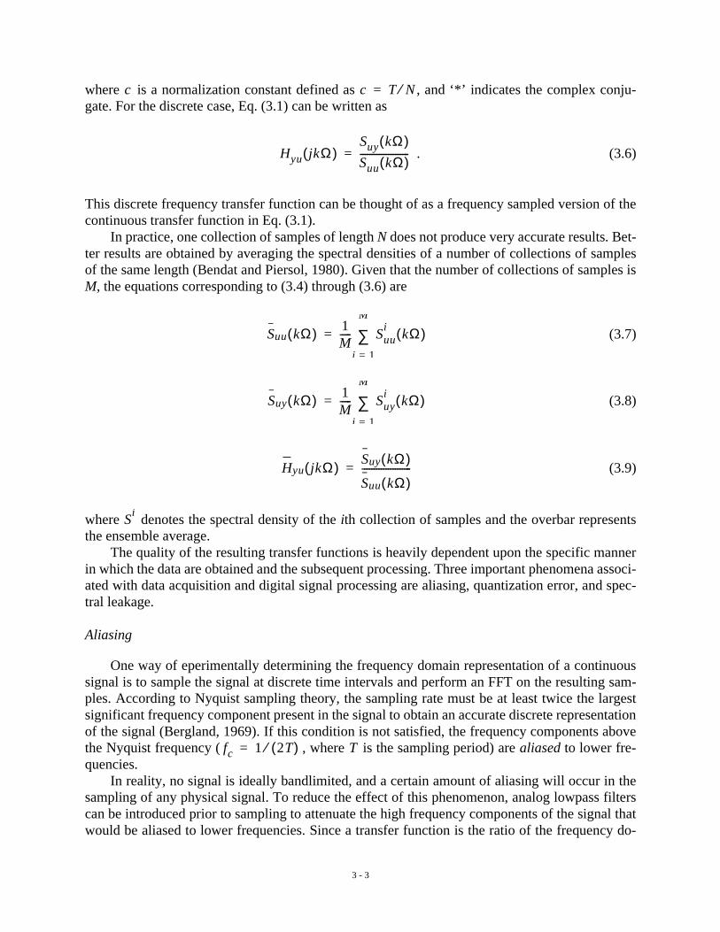
Figures 3.2–3.4 show representative magnitude and phase plots for the experimentally deter-mined transfer functions. All transfer functions were obtained using twenty averages. Figure 3.2presents the transfer function from the ground acceleration to the first floor acceleration (with the input to the control actuator set to zero). Note the three distinct, lightly-damped modesoccurring in each of the transfer functions. These peaks occur at 2.33 Hz, 7.37 Hz, and 12.24 Hzand correspond to the first three modes of the structural system. Similarly, the experimental trans-fer function from the control command u to the first floor acceleration (setting the input to theearthquake simulator to zero) is depicted in Fig. 3.3. Note the significant high frequency dynam-ics present; the magnitude of the transfer function at 40 Hz is as great as that corresponding to thebuilding’s primary modes. Clearly, these dynamic effects must be considered in the control de-sign.

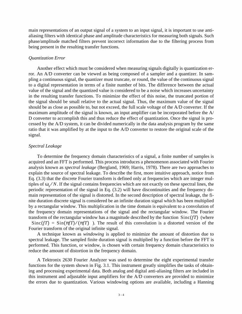
Figure 3.4 shows the transfer function from the actuator command u to the actuator displace-ment (i.e., the actuator transfer function). As expected, this transfer function has the same threelightly damped modes of the structural system that are seen in Figs. 3.2 and 3.3. In addition, thereare significant modes at high frequencies that correspond to actuator dynamics. These actuator

0 5 10 15 20 25 30 35 40 45 50-600

-400

-200

0

Experimental

Analytical

0 5 10 15 20 25 30 35 40 45 50-40

-20

0

20

40

Figure 3.2 Transfer Function from Ground Acceleration to First Floor Acceleration.

Frequency (Hz)

Frequency (Hz)

Mag

nitu

de (

dB)

Phas

e (d

eg)

x··g x··a1

x··a1

xa

3 - 6

Figure 3.3 Transfer Function from Actuator Command to First Floor Acceleration.

Frequency (Hz)

Frequency (Hz)

Mag

nitu

de (

dB)

Phas

e (d

eg)

0 5 10 15 20 25 30 35 40 45 50-500

-400

-300

-200

-100

0

Experimental

Analytical

0 5 10 15 20 25 30 35 40 45 50-80

-60

-40

-20

0

20

0 5 10 15 20 25 30 35 40 45 50-250

-200

-150

-100

-50

0

Experimental

Analytical

0 5 10 15 20 25 30 35 40 45 50-5

0

5

10

15

Figure 3.4 Transfer Function from Actuator Command to Actuator Displacement.

Frequency (Hz)

Frequency (Hz)

Mag

nitu

de (

dB)

Pha

se (

deg)

3 - 7

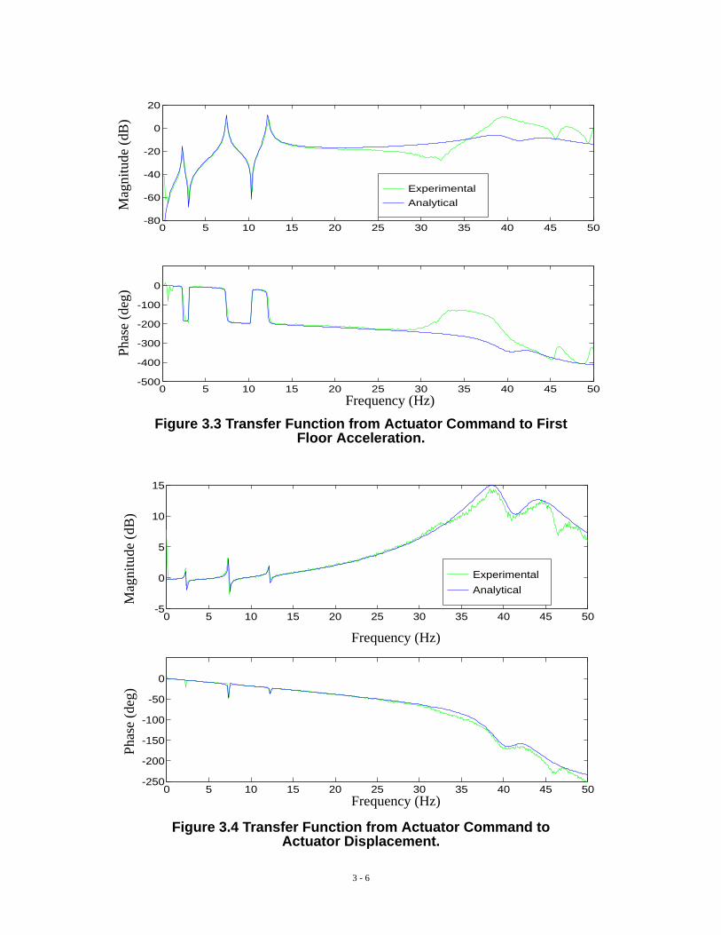
dynamics are the primary source of the high frequency dynamics seen in the transfer functions inFigs. 3.2 and 3.3. If the gain on the stabilization loop of the hydraulic actuator is reduced, thesehigh frequency dynamics are greatly reduced, although at the expense of a more slowly respond-ing actuator. To observe this effect, the actuator transfer function was experimentally determinedfor two different feedback gains. The two transfer functions are compared in Fig. 3.5. Notice thatreducing the feedback gain causes the actuator transfer function to roll off at a lower frequencyand the actuator dynamics to be highly damped.

3.2 Mathematical Modeling of Transfer Functions

Once the experimental transfer functions have been obtained, the next step in the systemidentification procedure is to model the transfer functions as a ratio of two polynomials in theLaplace variable s. This task was accomplished via a least squares fit of the ratio of numerator anddenominator polynomials, evaluated on the axis, to the experimentally obtained transfer func-tions (Schoukens and Pintelon, 1991). The algorithm requires the user to input the number ofpoles and zeros to use in estimating the transfer function, and then determines the location for thepoles/zeros and the gain of the transfer function for a best fit. This algorithm was used to fit eachof the eight transfer functions.

To effectively identify a structural model, a thorough understanding of the significant dy-namics of the structural system is required. For example, because the transfer functions representthe input/output relationships for a single physical system, a common denominator was assumed

0 5 10 15 20 25 30 35 40 45 50-250

-200

-150

-100

-50

0

gain = 7.5

gain = 9.5

0 5 10 15 20 25 30 35 40 45 50-10

0

10

20

Figure 3.5 Comparison of Actuator Transfer Functions for Various Feedback Gains.

Frequency (Hz)

Frequency (Hz)

Mag

nitu

de (

dB)

Phas

e (d

eg)

jω

3 - 8

for the elements of each column of the transfer function matrix. The curve fitting routine, howev-er, does not necessarily yield this result. Thus, the final locations of the poles and zeros were thenadjusted as necessary to more accurately represent the physical system. A MATLAB (1993) com-puter code was written to automate this process.

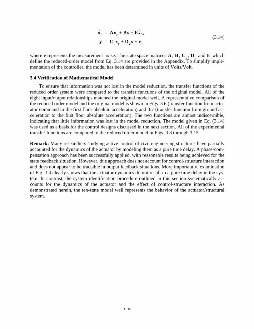
Another important phenomenon that should be consistently incorporated into the identifica-tion process is control-structure interaction. Most of the current research in the field of structuralcontrol does not explicitly take into account the effects of control-structure interaction in the anal-ysis and design of protective systems. Dyke, et al. (1993, 1994) have shown that the dynamics ofthe hydraulic actuators are integrally linked to the dynamics of the structure. By including the ac-tuator in the structural system, the actuator dynamics and control-structure interaction effects areautomatically taken into account in the experimental data. However, one must ensure that the ef-fects of control-structure interaction are not neglected in obtaining a mathematical model of theexperimental transfer functions.

For the system under consideration, the results in Dyke, et al. (1993, 1994) show that thepoles of the structure (including the active tendons) will appear as zeros of the transfer functionfrom the command input to the actuator displacement. This phenomenon occurs regardless of howfast (or slow) the actuator responds. The predicted behavior is clearly seen in Fig. 3.4, where thereis nearly a pole/zero cancellation at the first three modes of the structural system. These zeros cor-respond to the poles of the transfer function from the actuator displacement to the building re-sponses. The near cancellation of these poles and zeros occurs because the tendons applying thecontrol force to the structure are relatively flexible, as compared to the building stiffness. If onedid not anticipate the effect of control-structure interaction, the transfer function for the actuatorshown in Fig. 3.4 might have been assumed to be unity over the interval from 0–20 Hz. In addi-tion, the mass of the frame connecting the tendons to the actuator is not negligible and has a sig-nificant effect on the dynamics of the system. The frame must be viewed as an additional degree-of-freedom in the system. This extra degree-of-freedom was implicitly incorporated into the sys-tem model.

Of course, the structural system is actually a continuous system and will have an infinitenumber of vibrational modes. One of the jobs of the control designer is to ascertain which of thesemodes are necessary to model for control purposes. Herein, it was decided that the control of thefirst three modes was desired; thus the model of the system needed to be accurate to approximate-ly 20 Hz. However, a consequence of this decision is that significant control effort should not beapplied at frequencies above 20 Hz. The techniques used to roll-off the control effort at higher fre-quencies are presented in Section 4.

The mathematical models of the transfer functions are overlaid in Figs. 3.2–3.4. The identi-fied poles of the structural system are: , , ,

, , and (in Hz). The quality of the mathematical models forthe remaining transfer functions was similar to that depicted in Figs. 3.2–3.4.

3.3 State Space Realization

The system was then assembled in a state space form using the analytical representation ofthe transfer functions (i.e., the poles, zeros and gain) for each individual transfer function. Be-cause the system under consideration is a multi-input/multi-output system (MIMO), such a con-struction was not straightforward.

0.005– 2.33j± 0.030– 7.37j± 0.050– 12.24j±2.01– 39.22j± 3.03– 43.26j± 140–

3 - 9

First, two separate systems are formed, each with a single input corresponding to one of thetwo inputs to the system. The state equations modeling the input/output relationship between thedisturbance, , and the measured outputs can be realized as

(3.10)

where , , , and are in controller canonical form, is the state vector, and the vectorof measured structural responses is given by . Because the transfer func-tion characteristics from the ground to the building response were dominated by the dynamics ofthe building (see Fig. 3.2), the system in Eq. (3.10) required only six states, corresponding to thethree modes of the building, to accurately model the experimental transfer function over the fre-quency range of interest.

The second state equations, modeling the input/output relationship between the actuator com-mand u and the responses y are given by

(3.11)

where , , , and are in controller canonical form, and is the state vector. This sys-tem contains eleven states corresponding to the eleven poles identified in the previous section.

Once both of the component system state equations have been identified, the MIMO systemcan be formed by stacking the states of the two individual systems. By defining a new state vec-tor, , the state equation for the two-input/four-output system is written

, (3.12)

and the measurement equation becomes

. (3.13)

However, this is not a minimum realization of the system. The dynamics of the test structure itselfare redundantly represented in this combined state space system, thus the 17 state system given inEqs. 3.12 and 3.13 had repeated eigenvalues for which the eigenvectors were not linearly inde-pendent (i.e., the associated modes are not linearly independent). Thus, a balanced realization ofthe system given in Eqs. (3.12) and (3.13) was found and a model reduction was performed(Moore, 1981; Laub, 1980). The system model was reduced to a tenth-order system. Six of theeliminated states corresponded to the six redundant states corresponding to the building dynam-ics. The additional state that was eliminated corresponded to the very fast pole at 140 Hz found inthe original system identification. The state space representation of the reduced model is given by

x··g

x·1 A1x1 B1x··g,+=

y C1x1 D1x··g,+=

A1 B1 C1 D1 x1y xa x··a1 x··a2 x··a3[ ]′=

x· 2 A2x2 B2u,+=

y C2x2 D2u.+=

A2 B2 C2 D2 x2

x x1 x2[ ]′=

x·A1 0

0 A2

x0

B2

uB1

0x··g+ +=

y C1 C2 x D2u D1x··g+ +=

3 - 10

(3.14)

where v represents the measurement noise. The state space matrices , , , and whichdefine the reduced-order model from Eq. 3.14 are provided in the Appendix. To simplify imple-mentation of the controller, the model has been determined in units of Volts/Volt.

3.4 Verification of Mathematical Model

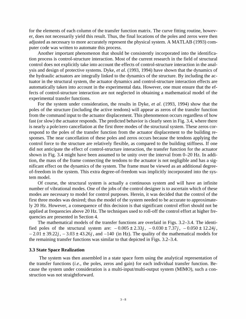
To ensure that information was not lost in the model reduction, the transfer functions of thereduced order system were compared to the transfer functions of the original model. All of theeight input/output relationships matched the original model well. A representative comparison ofthe reduced order model and the original model is shown in Figs. 3.6 (transfer function from actu-ator command to the first floor absolute acceleration) and 3.7 (transfer function from ground ac-celeration to the first floor absolute acceleration). The two functions are almost indiscernible,indicating that little information was lost in the model reduction. The model given in Eq. (3.14)was used as a basis for the control designs discussed in the next section. All of the experimentaltransfer functions are compared to the reduced order model in Figs. 3.8 through 3.15.

Remark: Many researchers studying active control of civil engineering structures have partiallyaccounted for the dynamics of the actuator by modeling them as a pure time delay. A phase-com-pensation approach has been successfully applied, with reasonable results being achieved for thestate feedback situation. However, this approach does not account for control-structure interactionand does not appear to be tractable in output feedback situations. More importantly, examinationof Fig. 3.4 clearly shows that the actuator dynamics do not result in a pure time delay in the sys-tem. In contrast, the system identification procedure outlined in this section systematically ac-counts for the dynamics of the actuator and the effect of control-structure interaction. Asdemonstrated herein, the ten-state model well represents the behavior of the actuator/structuralsystem.

x· r Axr Bu Ex··g,+ +=

y Cyxr Dyu v,+ +=

A B Cy Dy E

3 - 11

0 5 10 15 20 25 30 35 40 45 50-80

-60

-40

-20

0

20

Original ModelReduced Model

0 5 10 15 20 25 30 35 40 45 50-400

-300

-200

-100

0

Frequency (Hz)

Frequency (Hz)

Mag

nitu

de (

dB)

Pha

se (

deg)

Figure 3.6 Comparison of the Reduced Order Model and Original Model Transfer Functions: Actuator Command to the First Floor Acceleration.

3 - 12

Figure 3.7 Comparison of the Reduced Order Model and Original Model Transfer Functions: Ground Acceleration to the First Floor Acceleration.

0 5 10 15 20 25 30 35 40 45 50-40

-20

0

20

40

Original ModelReduced Model

0 5 10 15 20 25 30 35 40 45 50-200

-100

0

100

Frequency (Hz)

Frequency (Hz)

Mag

nitu

de (

dB)

Phas

e (d

eg)

0 5 10 15 20 25 30 35 40 45 50-250

-200

-150

-100

-50

0

ExperimentalAnalytical

0 5 10 15 20 25 30 35 40 45 50-10

0

10

20

Figure 3.8 Comparison of Reduced-Order Model and Experimental Transfer Function from the Actuator Command to the Actuator Displacement.

Frequency (Hz)

Frequency (Hz)

Mag

nitu

de (

dB)

Pha

se (

deg)

3 - 13

0 5 10 15 20 25 30 35 40 45 50-500

-400

-300

-200

-100

0


0 5 10 15 20 25 30 35 40 45 50-80

-60

-40

-20

0

20

Frequency (Hz)

Frequency (Hz)

Mag

nitu

de (

dB)

Pha

se (

deg)

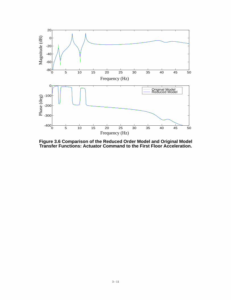
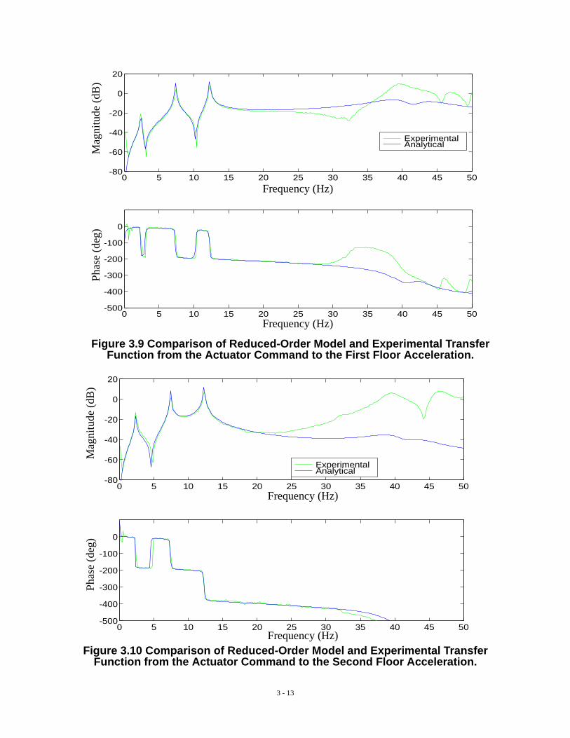
Figure 3.9 Comparison of Reduced-Order Model and Experimental Transfer Function from the Actuator Command to the First Floor Acceleration.

0 5 10 15 20 25 30 35 40 45 50-500

-400

-300

-200

-100

0


0 5 10 15 20 25 30 35 40 45 50-80

-60

-40

-20

0

20

Figure 3.10 Comparison of Reduced-Order Model and Experimental Transfer Function from the Actuator Command to the Second Floor Acceleration.

Frequency (Hz)

Frequency (Hz)

Mag

nitu

de (

dB)

Pha

se (

deg)

3 - 14

0 5 10 15 20 25 30 35 40 45 50-800

-600

-400

-200

0

200


0 5 10 15 20 25 30 35 40 45 50-60

-40

-20

0

20

Figure 3.11 Comparison of Reduced-Order Model and Experimental Transfer Function from the Actuator Command to the Third Floor Acceleration.

Frequency (Hz)

Frequency (Hz)

Mag

nitu

de (

dB)

Pha

se (

deg)

0 5 10 15 20 25 30 35 40 45 50-800

-600

-400

-200

0

200


0 5 10 15 20 25 30 35 40 45 50

-40

-20

0

20

Figure 3.12 Comparison of Reduced-Order Model and Experimental Transfer Function from the Ground Acceleration to the Actuator Displacement.

Frequency (Hz)

Frequency (Hz)

Mag

nitu

de (

dB)

Pha

se (

deg)

3 - 15

0 5 10 15 20 25 30 35 40 45 50-600

-400

-200

0


0 5 10 15 20 25 30 35 40 45 50-40

-20

0

20

40

Figure 3.13 Comparison of Reduced-Order Model and Experimental Transfer Function from the Ground Acceleration to the First Floor Acceleration.

Frequency (Hz)

Frequency (Hz)

Mag

nitu

de (

dB)

Phas

e (d

eg)

0 5 10 15 20 25 30 35 40 45 50-600

-400

-200

0


0 5 10 15 20 25 30 35 40 45 50

-40

-20

0

20

Figure 3.14 Comparison of Reduced-Order Model and Experimental Transfer Function from the Ground Acceleration to the Second Floor Acceleration.

Frequency (Hz)

Frequency (Hz)

Mag

nitu

de (

dB)

Pha

se (

deg)

3 - 16

0 5 10 15 20 25 30 35 40 45 50-800

-600

-400

-200

0


0 5 10 15 20 25 30 35 40 45 50-80

-60

-40

-20

0

20

Figure 3.15 Comparison of Reduced-Order Model and Experimental Transfer Function from the Ground Acceleration to the Third Floor Acceleration.

Frequency (Hz)

Frequency (Hz)

Mag

nitu

de (

dB)

Pha

se (

deg)

4 - 1

SECTION 4

CONTROL DESIGN

In control design, a trade-off exists between good performance and robust stability. Betterperformance usually requires a more authoritative controller. However, uncertainties in the sys-tem model may result in severely degraded performance and perhaps even instabilities if the con-troller is too authoritative. Therefore, the uncertainties in the model are a limiting factor in theperformance of the control system. Spencer, et al. (1994c) have shown that H2/LQG design meth-ods produce effective controllers for this class of problems. For the sake of completeness, a briefoverview of /LQG control design methods is given below.

4.1 Control Algorithm

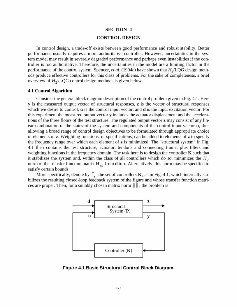
Consider the general block diagram description of the control problem given in Fig. 4.1. Herey is the measured output vector of structural responses, z is the vector of structural responseswhich we desire to control, u is the control input vector, and d is the input excitation vector. Forthis experiment the measured output vector y includes the actuator displacement and the accelera-tions of the three floors of the test structure. The regulated output vector z may consist of any lin-ear combination of the states of the system and components of the control input vector u, thusallowing a broad range of control design objectives to be formulated through appropriate choiceof elements of z. Weighting functions, or specifications, can be added to elements of z to specifythe frequency range over which each element of z is minimized. The “structural system” in Fig.4.1 then contains the test structure, actuator, tendons and connecting frame, plus filters andweighting functions in the frequency domain. The task here is to design the controller K such thatit stabilizes the system and, within the class of all controllers which do so, minimizes the norm of the transfer function matrix from d to z. Alternatively, this norm may be specified tosatisfy certain bounds.

More specifically, denote by the set of controllers , as in Fig. 4.1, which internally sta-bilizes the resulting closed-loop feedback system of the figure and whose transfer function matri-ces are proper. Then, for a suitably chosen matrix norm , the problem is

H2

StructuralSystem (P)

Controller (K)

u y

zd

Figure 4.1 Basic Structural Control Block Diagram.

H2Hzd

Îs K

.

4 - 2

(4.1)

To obtain the transfer function , we refer to Fig. 4.1 and partition the system transfer functionmatrix into its components, i.e.,

. (4.2)

The overall transfer function from to can then be written as (Suhardjo, 1990),

. (4.3)

As with , it is assumed that in Eq. (4.2) is proper. The reader should also note that the inversein Eq. (4.3) must exist. For simplicity, this latter requirement may be included in the definition of

. Because may include appropriate filters and weighting functions in the frequency domain,as described above, it is clear that will embody them as well.

The controller resulting from Eqs. (4.1) and (4.3) will depend upon the norm employed in theminimization. As suggested by the name, the control design searches for a stabilizing control-ler which minimizes the norm of , . The norm of a stable transfer function ma-trix is defined as (Boyd and Barratt, 1991)

. (4.4)

More physical insight into the meaning of the norm can be obtained by noting that the norm of a transfer function measures the root mean square (rms) value of its output, in a vec-

tor sense, when the input is a unit white noise excitation vector. The rms output vector is definedby

(4.5)

where for ease of notation, the symbol is used for both the time function and its transform.When is an ergodic stochastic process, Eq. (4.5) can also be written as

, (4.6)

min Hzd .K Îs∈

HzdP

PPzd Pzu

Pyd Pyu

=

d z

Hzd Pzd PzuK I PyuK–( ) 1–Pyd+=

K P

Îs PHzd

H2H2 Hzd Hzd 2 H2

H

H 2 trace1

2π------ H jω( )H* jω( )dω∞–

∞

∫

≡

H2H2

d rms12τ-----

τ ∞→lim dT

t( )d t( )dt

τ–

τ

∫=

dd t( )

d rms Ei∑ di

2 t( )[ ]=

4 - 3

where is the expected value operator.To illustrate these concepts, consider a structure under one-dimensional earthquake excita-

tion and active control input u. The structural system, which includes the structure, the actua-tor and any components required to apply the control force, can be represented in state space formas

(4.7)

(4.8)

where is the state vector of the system, is the vector of measured responses, and v representsthe noise in the measurements. A detailed block diagram representation of the system given inEqs. (4.7) and (4.8) is depicted in Fig. 4.2. In this figure, the transfer function G is given by

(4.9)

The filter F shapes the spectral content of the disturbance modeling the excitation, and areconstant matrices that dictate the components of structural response comprising the measured out-put vector y and the regulated response vector z, respectively. The matrix weighting functions

and are generally frequency dependent, with weighting the components ofregulated response and weighting the control force vector u. The input excitation vector dconsists of a white noise excitation vector w and a measurement noise vector v. The scalar param-eter k is used to express a preference in minimizing the norm of the transfer function from w to zversus minimizing the norm of the transfer function from v to z. For this block diagram represen-tation, the partitioned elements of the system transfer function matrix P in Eq. (4.2) are given by

E .[ ]

x··g

x· Ax Bu Ex··g+ +=

y Cyx Dyu v+ +=

x y

u

P

k F

Cy+

+

Cz

y

z2

z1

v

wd

Dy

G

α2W2

α1W1

Figure 4.2 Typical structural control block for a seismically excited structure.

K

G sI A–( ) 1–B˜

sI A–( ) 1–B E[ ] [G1 G2].= = =

Cy Cz

α1W1 α2W2 α1W1α2W2

4 - 4

, (4.10)

, (4.11)

, (4.12)

and

. (4.13)

Equations (4.10)–(4.13) can then be substituted into Eq. (4.3) to yield an explicit expression for. The solution of the control problem can now be solved via standard methods (cf., Su-

hardjo, 1990; Spencer, et al., 1994a).

4.2 Design Considerations and Procedure

To offer a basis for comparison, 21 candidate controllers were designed using /LQG con-trol design techniques, each employing a different performance objective. Designs which mini-mize either displacements relative to the foundation, interstory displacements or absoluteaccelerations of the structure were considered. Control designs were also considered which direct-ly used the measured earthquake accelerations in control action determination. In this case, thematrix in Eq. (4.13) included an additional term due to the measurement of the disturbance. In allof the controller designs considered, the weighting function on the regulated output, , andthe weighting function on the control force, , were constant matrices (i.e., independent offrequency). The earthquake filter F was modeled based on the Kanai–Tajimi spectrum. The per-formance of all of the candidate controllers was evaluated analytically and experimentally.

In Section 3, we indicated that the model on which the control designs were based was ac-ceptably accurate below 20 Hz, but that significant modeling errors occurred at higher frequen-cies, particularly near the dominant actuator dynamics (~40 Hz). If one tries to affect highauthority control at frequencies where the system model is poor, catastrophic results may occur.Thus, for the structural system under consideration, no significant control effort was allowedabove 20 Hz.

The loop gain transfer function was examined in assessing the various control designs. Here,the loop gain transfer function is defined as the transfer function of the system formed by break-ing the control loop at the input to the system, as shown in Fig. 4.3. Using the plant transfer func-tion given in Eq. (4.12), the loop gain transfer function is given as

(4.14)

Pzd

Pz1w Pz1v

Pz2w Pz2v

kα1W1CzG2F 0

0 0= =

Pzu

Pz1u

Pz2u

α1W1CzG1

α2W2

= =

Pyu CyG1 Dy+=

Pyd Pyw Pyv kCyG2F I= =

Hzd H2

H2

α1W1α2W2

Hloop KPyu K CyG1 Dy+( )= =

4 - 5

By “connecting” the measured outputs of the analytical system model to the inputs of the mathe-matical representation of the controller, the loop gain transfer function from the actuator com-mand input to the controller command output was calculated.

The loop gain transfer function was used to provide an indication of the closed-loop stabilitywhen the controller is implemented on the physical system. For stability purposes, the loop gainshould be less than one at the higher frequencies where the model poorly represents the structuralsystem (i.e., above 20 Hz). Thus, the magnitude of the loop gain transfer function should roll offsteadily and be well below unity at higher frequencies. Herein, a control design was considered tobe acceptable for implementation if the magnitude of the loop gain at high frequencies was lessthan -5 dB at frequencies greater than 20 Hz.

Figure 4.3 Diagram Describing the Loop Gain Transfer Function.

StructuralSystem (P)

Controller (K)

u

yd

u

Loop Gain Output

Loop Gain Input

5 - 1

SECTION 5

CONTROL IMPLEMENTATION

The controllers used in this experiment were implemented on digital computers. There aremany issues that must be understood and addressed to successfully implement a control design ona computer. The resolution of these issues typically dictates that relatively high sampling ratesneed to be attained. Recently developed hardware based on dedicated DSP chips allows for veryhigh sampling rates and offers new possibilities for control algorithm implementation.

A description of the digital control hardware used in this experiment is discussed below.Practical aspects of digital control implementation are also given. Further discussion of imple-mentation concepts is provided in Spencer, et al. (1994b) and Quast, et al. (1994). Finally, exper-imental verification of successful digital implementation of the controllers used is presented.

5.1 Digital Controller Hardware

One typical way in which digital control schemes were implemented in the past was throughthe use of data acquisition boards in the expansion bus of a personal computer (PC). In this con-figuration, the data acquisition board would be programmed or commanded to take samples ofsystem measured quantities at regular intervals. When available, the samples of the measuredquantities would be passed to the PC’s main CPU through the I/O space of the PC. The PC wouldthen perform the arithmetic calculations required for implementation of the digital filter and for-ward the results through the I/O space to the D/A devices for output conversion. These continu-ous-time signals would then be used as the control inputs to the plant.

This configuration has many drawbacks. The time required to perform all of the A/D and D/A operations and pass these quantities over the I/O space of the PC, as well as perform the controlalgorithm computations on the PC, may require undesirably large sampling periods and induceunacceptable time delays. Also, with such an equipment configuration, it is difficult to create ascheme which allows the operator to monitor and interact with the controller while the PC is en-gaged in performing the control computations.

A more powerful arrangement for implementation of a digital control system is realizablethrough the use of one of many different DSP boards available that are placed in the expansionbus of a personal computer. State of the art DSP chips allow for very fast computational speedsas well as dedicated processing. The DSP boards have A/D and D/A converters locally on theboard which reduces the delay involved in the transmission of signals between the processor andthe I/O devices. Further, such configurations enable the control and monitoring of the DSP boardby the PC in a supervisory control scheme.

The control system employed in this experiment utilized the Real-Time Digital Signal Pro-cessor System made by Spectrum Signal Processing, Inc. It is configured on a board that plugsinto a 16-bit slot in a PC’s expansion bus and features a Texas Instruments TMS320C30 DigitalSignal Processor chip, RAM memory and on board A/D and D/A systems. The TMS320C30 DSPchip has single-cycle instructions, a 33.3 MHz clock, a 60 ns instruction cycle and can achieve anominal performance of 16.7 MFLOPS. A special feature of the chip that allows a floating pointmultiplier and adder to be used in parallel yields a theoretical peak performance of 33.3MFLOPS. Moreover, this board has a number of built-in functions that make it ideal for controlapplications. For example, there are notch filters to cancel mechanical resonances, adaptive Kal-man filter algorithms to reduce sensor noise, vector control algorithms for real-time axis transfor-mation and fuzzy set control algorithms.

5 - 2

In addition, the on-board A/D system has two channels, each with 16 bit precision and a max-imum sampling rate of 200 kHz. The two D/A channels, also with 16 bit precision, allow for evengreater output rates so as not to be limiting. An expansion I/O daughter board, which connects di-rectly to the DSP board, provides an additional four channels of input and two channels of outputcapability, each with 12 bit precision. All four input channels share the same conversion device,which is the limiting factor for the board’s sampling rate. The maximum sampling rate for thedaughter board is 200 kHz for one channel and proportionally less for multiple channels, with arate of 50 kHz per channel if all four channels are used. The maximum rate for each of the twodaughter board output channels is 300k samples/second. Additional daughter cards may be addedto the system to further expand the system’s I/O capabilities. Clearly, with the high computationrates of the DSP chip and the extremely fast sampling and output capability of the associated I/Osystem, high overall sampling rates for the digital control system are achievable.

As mentioned previously, the board plugs into a 16 bit expansion slot in a PC, which allowsfor communication between the DSP board and the PC through the I/O space of the PC. The PC isused to download the control code to the DSP board through this I/O interface. Further, while theDSP board runs the control algorithm, a supervisory program running on the PC can monitor theperformance of the control system, monitor and display measured quantities, and allow the opera-tor to send commands to the DSP board, starting and stopping the controller or changing controlparameters. This configuration allows for a very powerful and flexible implementation of a digitalcontrol system for structural control.

5.2 Digital Control System Design

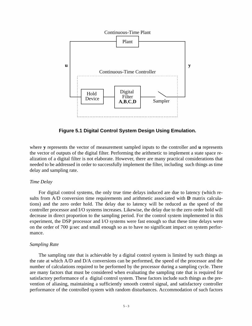
The method of “emulation” was used for the design of the discrete-time controller (Quast, et.al., 1994). Using this technique, a continuous-time controller was first designed which producedsatisfactory control performance. The continuous-time controller was then approximated or `emu-lated' with a discrete-time equivalent digital filter using the bilinear transformation. This configu-ration is illustrated in Figure 5.1. The controller samples the measured outputs of the plant andpasses the samples through a digital filter implemented on the DSP board. The output of the digi-tal filter was then passed through a hold device to create a continuous-time signal which becamethe control input to the plant. The series combination of sampler, digital filter and hold emulatedthe operation of a continuous-time controller. Typically, with the use of emulation, if the sam-pling rate of the digital controller is greater than about 10-25 times the closed-loop system band-width, the discrete equivalent system will adequately represent the behavior of the emulatedcontinuous-time system over the frequency range of interest. This sampling rate was successfullyachieved by the DSP system used in this experiment.

5.3 Digital Control Implementation Issues

Once a filter was designed for use in the digital control system, it was implemented on a DSPsystem using state space form:

(5.1)

(5.2)

x kT T+( ) Ax kT( ) By kT( )+=

u kT( ) Cx kT( ) Dy kT( )+=

5 - 3

where y represents the vector of measurement sampled inputs to the controller and u representsthe vector of outputs of the digital filter. Performing the arithmetic to implement a state space re-alization of a digital filter is not elaborate. However, there are many practical considerations thatneeded to be addressed in order to successfully implement the filter, including such things as timedelay and sampling rate.

Time Delay

For digital control systems, the only true time delays induced are due to latency (which re-sults from A/D conversion time requirements and arithmetic associated with D matrix calcula-tions) and the zero order hold. The delay due to latency will be reduced as the speed of thecontroller processor and I/O systems increases. Likewise, the delay due to the zero order hold willdecrease in direct proportion to the sampling period. For the control system implemented in thisexperiment, the DSP processor and I/O systems were fast enough so that these time delays wereon the order of 700 sec and small enough so as to have no significant impact on system perfor-mance.

Sampling Rate

The sampling rate that is achievable by a digital control system is limited by such things asthe rate at which A/D and D/A conversions can be performed, the speed of the processor and thenumber of calculations required to be performed by the processor during a sampling cycle. Thereare many factors that must be considered when evaluating the sampling rate that is required forsatisfactory performance of a digital control system. These factors include such things as the pre-vention of aliasing, maintaining a sufficiently smooth control signal, and satisfactory controllerperformance of the controlled system with random disturbances. Accommodation of such factors

Plant

Hold Device

Digital Filter

Sampler

Continuous-Time Controller

Continuous-Time Plant

Figure 5.1 Digital Control System Design Using Emulation.

yu

A,B,C,D

µ

5 - 4

usually requires a sampling rate of the controller that is 10-25 times greater than the significantfrequencies in the measured responses, depending on the specific application. For this experi-ment, all I/O processes, control calculations, and supervisory functions were performed in lessthan 1 msec, allowing for sampling rates on the order of 1 kHz. Thus, the TMS320C30 DSP sys-tem readily accommodated this sampling rate guidance.

5.4 Software

Once the controller digital filter is designed, it is implemented using the Real-Time DigitalSignal Processor System. The code for these programs can be written directly in the C program-ming language. The code is compiled, linked with library functions and made into executable fileson the PC. The PC is then used to download the control code to the DSP board through the PC’sI/O interface. The SPOX operating system provides standard I/O library support for the C lan-guage so that pre-existing C programs will execute with limited code modification. SPOX alsoprovides a library of standard DSP functions which free the operator from writing lower levelcode such as device drivers for managing incoming data. Applications written in C under SPOXare portable to other hardware environments supporting SPOX.

In addition to the implementation of the control algorithm difference equations (Eqs. (5.1)and (5.2)), several other tasks are performed on the DSP board during controller operation. In par-ticular, standard deviations are calculated for all measured quantities. These values are read itera-tively by the supervisory program running on the PC and are continuously displayed on the PCdisplay so the operator can monitor performance of the system. Further, as is done extensively incontrol system implementation in general as well as in structural control, at each sample instant,the magnitudes of certain measured quantities such as the actuator force and displacement arecompared to maximum allowable values specified by the user (Soong, et al., 1991; Reinhorn, etal., 1993). If at any instant the measured values exceed the maximum allowable values, the con-troller is immediately shut off and the command signal is set equal to zero. In addition, if the com-mand output calculated by the control algorithm exceeds the range of the D/A devices, acontroller shutdown also occurs. In this case, if the controller were allowed to continue to operatewith a saturated command output, the control signal would effectively be corrupted by a noise sig-nal equal in magnitude to the difference between the commanded output and the saturation levelof the D/A device. Such a situation could have devastating effects on the performance and stabili-ty of the system.

If a shutdown occurs, the supervisory program on the PC, repeatedly checking the conditionof the controller, detects the shutdown and displays an advisory on the monitor for the operator.This feature is designed to protect the system and structure from damage due to excessive or un-stable response caused by modeling errors, high ground excitation or mistakes in the hardware orsoftware implementation of the controller. The supervisory program running on the PC also al-lows the operator to turn the controller on and off as well as to change control parameters of thecontroller during its operation. Although changing parameters in the control algorithm while thecontroller is running may be desirable in some cases, it is generally not advisable unless a carefulassessment is made of the effects of such changes during control operation.

5.5 Verification of Digital Controller

After the data that was used for system identification was collected, a period of several weekselapsed before the controllers were actually implemented. Before implementing the controllers,

5 - 5

the transfer functions of the system were again determined to verify that the system model onwhich the controller designs were based was still valid. During the time between the system iden-tification tests and implementation of the control designs the structural system softened, resultingin approximately a 1% decrease in the frequencies of the first three modes. However, the controldesigns were robust enough to account for the slight differences. All of the twenty-one control de-signs which were implemented produced a significant reduction in the responses. Ten of the con-trollers were thoroughly tested with various excitations, and the results of five representativecontrollers are provided in the following section.

Extensive testing was conducted for all components of the control hardware and software be-fore the experiments on the controlled structure were performed. One of the final tests was to ex-perimentally determine the loop gain transfer function by attaching the measured outputs from thebuilding to the inputs of the controller (i.e., the DSP board). The loop gain transfer function wasthen calculated by exciting the actuator command input with a broadband excitation and measur-ing the controller output. Figure 5.2 compares the experimental and analytical loop gain transferfunctions for one of the test controllers (Controller E as defined in Table 6.1). The two transferfunctions are nearly identical below 40 Hz, indicating that the controller was working as expectedand the system model was accurate.

experimentalanalytical

0 5 10 15 20 25 30 35 40 45 50-40

-20

0

20

0 5 10 15 20 25 30 35 40 45 50-1200

-1000

-800

-600

-400

-200

Figure 5.2 Experimental Loop Gain at the Input for Controller E.

Frequency (Hz)

Frequency (Hz)

Mag

nitu

de (

dB)

Pha

se (

deg)

5 - 6

Note that except for built-in high frequency anti-aliasing filters on the input channels to theDSP board, no external filters were employed for either the feedback measurements or the controlsignal. All of the required frequency shaping was performed within the digital control algorithm.

6 - 1

SECTION 6

EXPERIMENTAL RESULTS

Two different types of tests were conducted on the earthquake simulator to verify the controldesigns. A bandlimited white noise ground excitation (0-10 Hz) was first used to excite the struc-ture to observe the ability of the controllers to reduce the rms values of the structural responses. Inthe second type of test, the earthquake simulator reproduced a recorded accelerogram to deter-mine the ability of the controllers to reduce the peak structural responses. For this test, two earth-quakes were chosen for controller verification: 1) an El Centro earthquake excitation (N-Scomponent) and 2) a Taft earthquake excitation (North 21 East component). The magnitude of theearthquakes were reduced to one-quarter (El Centro) and one-half (Taft) of the recorded intensityto reduce the possibility of damaging the structure. Also, because the test structure was a scaledmodel of a prototype structure, similitude relations dictated that both earthquakes be reproducedat double the speed of the recorded earthquakes.

6.1 Development and Validation of Simulation Model

As discussed previously, the characteristics of the system changed slightly between the timethat the original data (used for control design) was taken and the controllers were implemented.After completion of the experiments, a revised simulation model was developed based on the datataken when the control experiments were conducted. This was the model used in all comparisonsbetween the analytical and experimental results. Using the eigenvectors of the system matrix forthe original model, and modified values for the eigenvalues from the new data, a revised systemmatrix was formed.

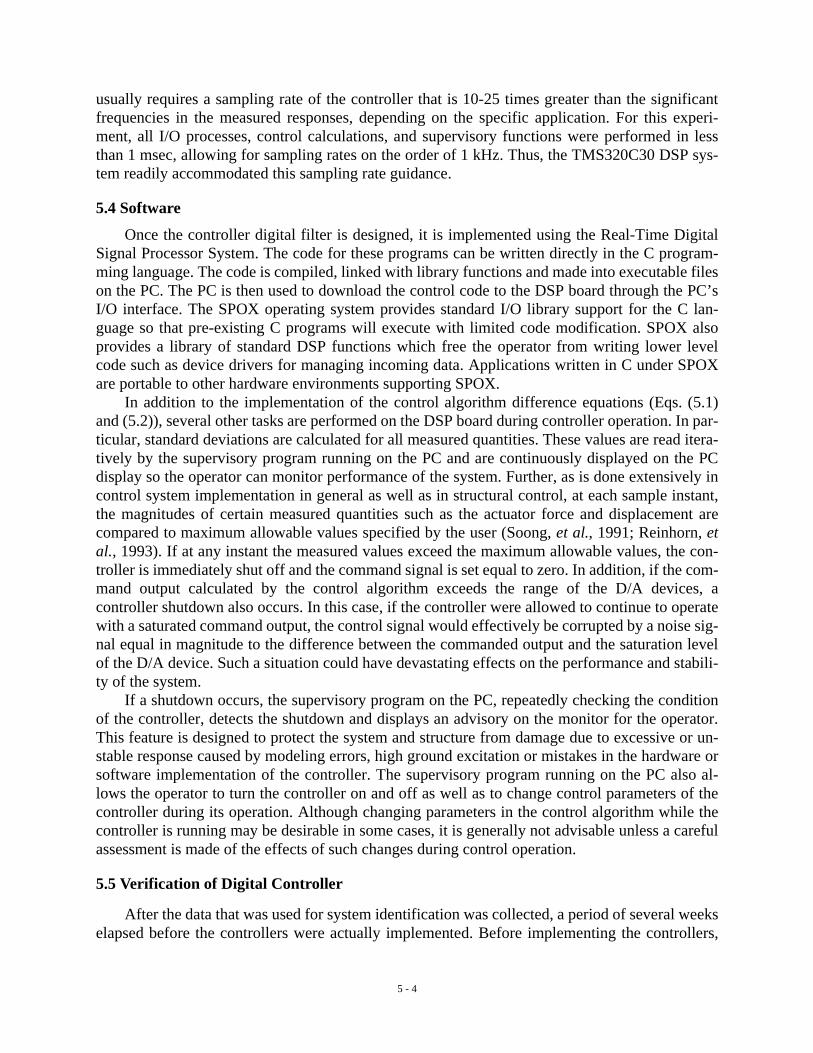
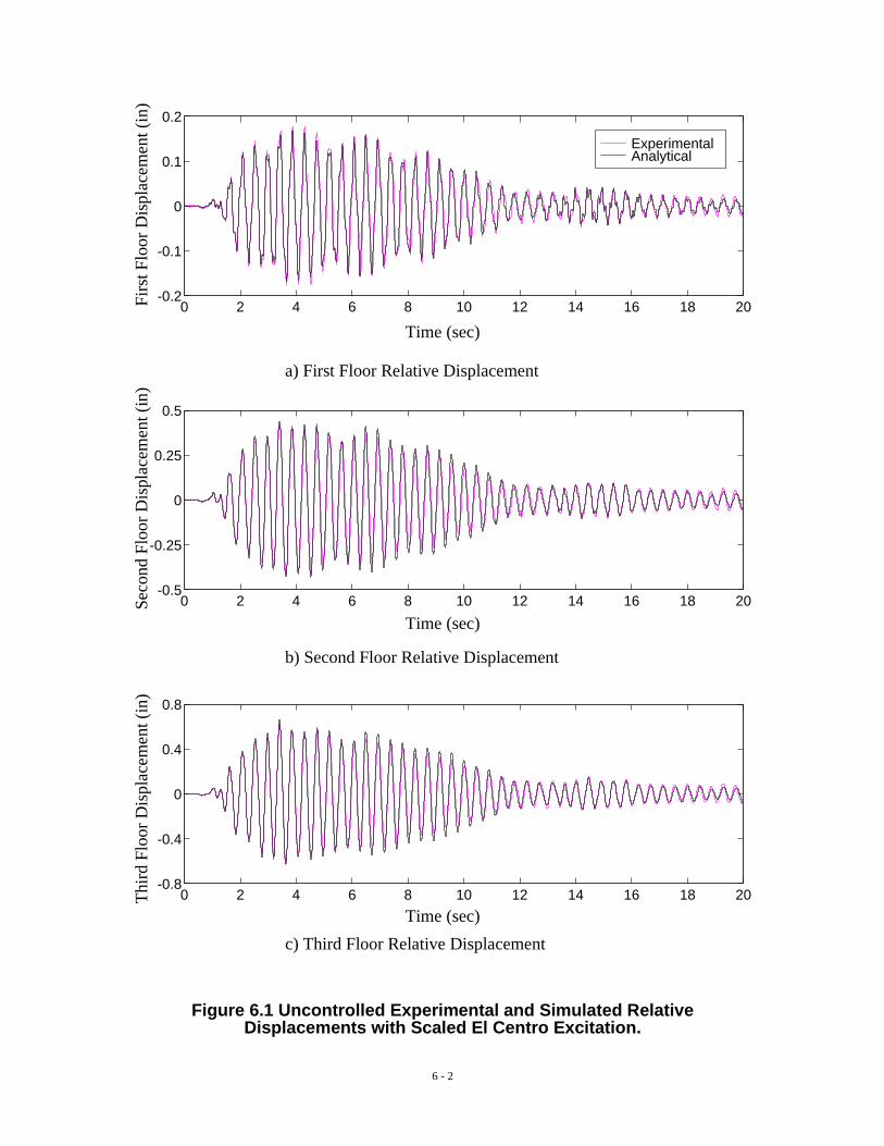
By exciting the model with the measured base accelerations, a simulation of the uncontrolledsystem was performed to verify the new model of the structural system. Uncontrolled, in this con-text, refers to the structural system with the tendons in place and the actuator command set to ze-ro. In Figs. 6.1a-c and 6.2a-c, the experimental and simulated time responses of the first, secondand third floor relative displacements and absolute accelerations for a quarter scale El Centro ex-citation are compared for verification of the simulation model. In all cases, the experimental andanalytical responses matched well, indicating that the simulation model is quite accurate. In addi-tion, the analytical loop gain shown in Fig. 5.2 corresponds to this model. The analytical and ex-perimental loop gains match well, indicating that the controller was operating as expected. Again,notice that the experimental and analytical loop gains match well in the frequency range of inter-est, indicating that the model is accurate and the control system is behaving as expected.

6.2 Discussion of Results and Comparison to Simulation

Twenty-one control designs were implemented, all of which were designed based on theoriginal model. Each controller performed well and none resulted in unstable systems. Ten of thecontrol designs were chosen for further study. The results of five representative control designs,designated A–E, are presented herein. Table 6.1 lists the five controllers with a description of thecorresponding control strategy employed for each design. The performance objective in the de-sign of Controller A was to minimize the relative displacements of the structure. This wasachieved by weighting the three displacements equally and applying a smaller weighting to theactuator displacement. Controller B was designed to minimize the interstory displacements. Inthis case a weighting matrix was chosen which corresponded to weighting the three interstory dis-

6 - 2


0 2 4 6 8 10 12 14 16 18 20-0.2

-0.1

0

0.1

0.2

0 2 4 6 8 10 12 14 16 18 20-0.5

-0.25

0

0.25

0.5

0 2 4 6 8 10 12 14 16 18 20-0.8

-0.4

0

0.4

0.8

Figure 6.1 Uncontrolled Experimental and Simulated Relative Displacements with Scaled El Centro Excitation.

c) Third Floor Relative Displacement

a) First Floor Relative Displacement

b) Second Floor Relative Displacement

Time (sec)

Time (sec)

Time (sec)

Firs

t Flo

or D

ispl

acem

ent (

in)

Seco

nd F

loor

Dis

plac

emen

t (in

)T

hird

Flo

or D

ispl

acem

ent (

in)

6 - 3

Firs

t Flo

or A

ccel

erat

ion

(g)

Seco

nd F

loor

Acc

eler

atio

n (g

)T

hird

Flo

or A

ccel

erat

ion

(g)


0 2 4 6 8 10 12 14 16 18 20-0.3

-0.2

-0.1

0

0.1

0.2

0.3

0 2 4 6 8 10 12 14 16 18 20-0.5

-0.25

0

0.25

0.5

0 2 4 6 8 10 12 14 16 18 20-0.4

-0.2

0

0.2

0.4

c) Third Floor Absolute Acceleration

a) First Floor Absolute Acceleration

b) Second Floor Absolute Acceleration

Figure 6.2 Uncontrolled Experimental and Simulated Absolute Accelerations with Scaled El Centro Excitation.

Time (sec)

Time (sec)

Time (sec)

6 - 4

placements and a smaller weighting was applied to the actuator displacement. The performance

objective in the design of Controller C was to minimize the absolute accelerations of the structure.This was achieved by placing equal weighting on all three absolute accelerations. Controller Dwas designed by weighting only the absolute acceleration of the third floor. Since the largest re-sponse in the fundamental mode is at the third floor, this approach serves to minimize all thestructural responses in the fundamental mode. In Controller E an additional measurement, thebase acceleration, was included in the measurement vector, and the absolute acceleration of thethird floor was weighted.

The experimental and simulated responses for Controllers A–E are provided in Tables 6.2,6.3 and 6.4. Table 6.2 provides rms responses of each controlled system to a broadband excitation(0-10 Hz) and Tables 6.3 and 6.4 report peak responses to the scaled El Centro and Taft excita-tions, respectively. Values for the absolute accelerations, , relative displacements, , intersto-ry displacements, actuator displacement, , and control signal, , are provided. The resultsinclude rms responses in the case of the bandlimited white noise excitation and peak responses forthe scaled El Centro and Taft excitations. The percent reduction of each controlled response rela-tive to the corresponding uncontrolled response is given in parentheses. Note the excellent agree-ment between the results predicted by the simulation and those obtained in the experiment. Theforce in the tendons (above the pretensioned value), f, was also measured during the experimentand is included in each table. Notice that the measured force in the tendons during the controlledtests was less than the force during the uncontrolled test for all control design.

Comparing Controllers A and B, it is evident that no particular advantage was gained byweighting interstory displacements in this experiment. In all response categories except the firstfloor displacement, Controller A consistently performed better than Controller B. In the first floorrelative displacement response, Controller B produced slightly better results than Controller A.However, Controller A reduced the remaining interstory displacements (i.e., and )5-10% more than Controller B. Also, Controller A reduced the rms relative displacements of each

Table 6.1: Description of Control Strategies for Each Design.

Controller Control Strategy

A Equal weighting on all three relative displacements and small weighting on the actuator displacement

B Weighting on the interstory displacements and small weighting on the actuator displacement

C Equal weighting on all three absolute accelerations

D Weighting on third floor absolute acceleration

E Weighting on third floor absolute acceleration and measurement of ground excitation

x··ai xixa uc

x2 x1– x3 x2–

6 - 5

Tab

le 6

.2:

RM

S R

esp

on

ses

of

Co

ntr

olle

d S

yste

m t

o B

road

ban

d E

xcit

atio

n.

Con

trol

ler

,,

,, i

n, i

n, i

nin

inf,

lbf

, in

Volt

s

Exp

erim

enta

l RM

S R

espo

nse

for

Ban

dlim

ited

Whi

te N

oise

Gro

und

Exc

itatio

n (1

0 H

z)

unco

ntro

lled

36.1

39.7

53.0

0.06

50.

161

0.22

80.

097

0.07

144

4.0

0.00

2—

A20

.5(4

3.2)

18.2

(54.

0)23

.8(5

5.1)

0.02

6(6

0.8)

0.06

1(6

1.9)

0.08

7(6

1.9)

0.03

7(6

1.5)

0.02

9(5

9.1)

183.

6(5

8.6)

0.00

80.

162

B17

.7(5

1.0)

18.2

(54.

1)24

.4(5

3.9)

0.02

8(5

7.0)

0.07

0(5

6.4)

0.10

0(5

6.2)

0.04

3(5

5.7)

0.03

2(5

5.1)

205.

6(5

3.7)

0.00

60.

125

C14

.1(6

1.0)

15.1

(62.

0)20

.3(6

1.6)

0.02

5(6

1.2)

0.06

2(6

1.7)

0.08

7(6

1.8)

0.03

7(6

1.7)

0.02

7(6

2.0)

170.

1(6

1.7)

0.00

80.

168

D13

.7(6

2.0)

13.8

(65.

3)18

.2(6

5.6)

0.02

4(6

4.0)

0.05

5(6

5.9)

0.07

7(6

6.4)

0.03

3(6

6.5)

0.02

4(6

6.6)

147.

2(6

6.8)

0.01

00.

210

E13

.5(6

2.7)

13.3

(66.

4)17

.5(6

7.0)

0.02

3(6

5.0)

0.05

3(6

7.2)

0.07

4(6

7.7)

0.03

1(6

7.9)

0.02

3(6

8.1)

141.

3(6

8.2)

0.01

10.

220

Sim

ulat

ion

RM

S R

espo

nse

for

Ban

dlim

ited

Whi

te N

oise

Gro

und

Exc

itatio

n (1

0 H

z)

unco

ntro

lled

34.7

39.5

52.5

0.05

90.

160

0.22

50.

104

0.07

141

3.6

0.00

2—

A19

.7(4

3.2)

18.6

(52.

9)22

.7(5

6.9)

0.02

5(5

7.8)

0.06

2(6

1.3)

0.08

7(6

1.4)

0.04

0(6

1.4)

0.02

9(5

8.7)

175.

4(5

7.6)

0.00

90.

187

B17

.0(5

0.8)

18.7

(52.

7)24

.3(5

3.8)

0.02

7(5

4.1)

0.07

2(5

4.9)

0.10

2(5

4.7)

0.04

7(5

4.7)

0.03

3(5

4.3)

195.

3(5

2.8)

0.00

70.

141

C13

.5(6

1.0)

15.3

(61.

2)20

.2(6

1.6)

0.02

5(5

7.3)

0.06

4(6

0.2)

0.08

9(6

0.6)

0.04

0(6

1.1)

0.02

7(6

1.9)

157.

9(6

1.8)

0.01

00.

195

D13

.1(6

2.1)

13.9

(64.

9)17

.7(6

6.4)

0.02

4(5

9.5)

0.05

6(6

4.9)

0.07

7(6

5.7)

0.03

5(6

6.6)

0.02

3(6

7.3)

134.

0(6

7.6)

0.01

30.

250

E12

.9(6

2.9)

13.4

(66.

1)16

.9(6

7.9)

0.02

3(6

0.1)

0.05

4(6

6.1)

0.07

4(6

7.2)

0.03

3(6

8.2)

0.02

2(6

8.9)

132.

8(6

7.9)

0.01

30.

266

x·· a1

in s2-----x·· a

2in s2-----

x·· a3

in s2-----x 1

x 2x 3

x 2x 1

–x 3

x 2–

x au c

6 - 6

Tab

le 6

.3:

Pea

k R

esp

on

ses

of

Co

ntr

olle

d S

yste

m t

o S

cale

d E

l Cen

tro

Exc

itat

ion

.

Con

trol

ler

,,

,, i

n, i

n, i

nin

inf,

lbf

, in

,Vo

lts

Exp

erim

enta

l Pea

k R

espo

nse

for

Qua

rter

Sca

le E

l Cen

tro

Ear

thqu

ake

Exc

itatio

n.

unco

ntro

lled

93.0

118.

715

8.6

0.17

80.

421

0.62

70.

273

0.20

911

560.

005

—

A68

.3(2

6.6)

64.6

(45.

5)97

.7(3

8.4)

0.10

0(4

4.1)

0.22

1(4

7.6)

0.31

8(4

9.4)

0.14

0(4

8.9)

0.11

5(4

4.8)

629.

6(4

5.5)

0.03

10.

625

B67

.2(2

7.7)

68.2

(42.

6)94

.6(4

0.3)

0.10

2(4

2.6)

0.26

3(3

7.5)

0.38

8(3

8.1)

0.16

7(3

8.9)

0.12

7(3

9.2)

698.

9(3

9.5)

0.02

40.

500

C55

.9(3

9.9)

57.8

(51.

3)84

.1(4

7.0)

0.09

5(4

6.6)

0.23

0(4

5.5)

0.33

3(4

6.9)

0.14

2(4

7.9)

0.10

4(5

0.5)

584.

0(4

9.5)

0.03

40.

688

D57

.3(3

8.5)

56.5

(52.

3)82

.2(4

8.2)

0.09

4(4

7.2)

0.21

1(5

0.0)

0.29

3(5

3.3)

0.12

9(5

2.9)

0.09

5(5

4.5)

495.

2(5

7.2)

0.04

10.

824

E51

.7(4

4.4)

53.3

(55.

0)78

.4(5

0.6)

0.09

3(4

7.8)

0.20

6(5

1.1)

0.28

4(5

4.7)

0.12

5(5

4.3)

0.09

1(5

6.3)

927.

5(1

9.8)

0.04

40.

284

Sim

ulat

ion

Peak

Res

pons

e fo

r Q

uart

er S

cale

El C

entr

o E

arth

quak

e E

xcita

tion.

unco

ntro

lled

99.1

103.

916

8.5

0.16

90.

438

0.66

00.

309

0.22

111

940.

006

—

A64

.1(3

5.3)

66.1

(36.

4)93

.7(4

4.4)

0.09

8(4

1.7)

0.22

5(4

8.8)

0.32

7(5

0.4)

0.15

3(5

0.5)

0.11

6(4

7.6

622.

2(4

7.9)

0.03

50.

700

B64

.1(3

5.3)

70.9

(31.

8)95

.6(4

3.3)

0.09

7(4

2.4)

0.26

5(3

9.5)

0.39

0(4

0.8)

0.18

3(4

0.8)

0.12

6(4

2.9)

692.

1(4

2.0)

0.02

70.

538

C52

.7(4

6.8)

59.4

(42.

8)81

.3(5

1.7)

0.09

3(4

4.6)

0.23

6(4

6.1)

0.34

1(4

8.3)

0.15

8(4

8.9)

0.10

6(5

2.1)

553.

2(5

3.7)

0.03

90.

770

D52

.9(4

6.6)

56.8

(45.

4)76

.2(5

4.8)

0.09

5(4

3.5)

0.21

4(5

1.1)

0.29

9(5

4.6)

0.14

0(5

4.7)

0.09

7(5

6.3)

474.

9(6

0.2)

0.04

80.

953

E48

.7(5

0.9)

51.8

(50.

2)72

.9(5

6.8)

0.09

4(4

4.2)

0.20

7(5

2.9)

0.28

7(5

6.4)

0.13

3(5

6.9)

0.09

3(5

8.0)

459.

8(6

1.5)

0.05

11.

026

x·· a1

in s2-----x·· a

2in s2-----

x·· a3

in s2-----x 1

x 2x 3

x 2x 1

–x 3

x 2–

x au c

6 - 7

Tab

le 6

.4:

Pea

k R

esp

on

se o

f C

on

tro

lled

Sys

tem

to

Sca

led

Taf

t E

arth

qu

ake

Exc

itat

ion

.

Con

trol

ler

,,

,, i

n, i

n, i

nin

inf,

lbf

, in

,Vo

lts

Exp

erim

enta

l Pea

k R

espo

nse

for

One

-Hal

f Sc

ale

Taft

Ear

thqu

ake

Exc

itatio

n.

unco

ntro

lled

102.

710

4.5

146.

40.

165

0.40

80.

585

0.24

80.

187

1079

0.00

5—

A55

.9(4

5.5)

55.6

(46.

8)98

.9(3

2.4)

0.08

6(4

8.0)

0.22

2(4

5.6)

0.34

1(4

1.8)

0.14

6(4

1.1)

0.12

2(3

4.9)

576.

2(4

6.6)

0.02

90.

617

B57

.3(4

4.2)

60.9

(41.

7)10

2.9

(29.

7)0.

099

(39.

9)0.

260

(36.

2)0.

390

(33.

4)0.

169

(32.

1)0.

134

(28.

4)65

7.4

(39.

0)0.

023

0.49

2

C49

.4(5

1.8)

52.1

(50.

1)84

.8(4

2.1)

0.08

3(4

9.4)

0.22

4(4

5.1)

0.33

3(4

3.2)

0.14

4(4

2.0)

0.11

2(4

0.2)

562.

9(4

7.8)

0.03

10.

629

D44

.5(5

6.7)

48.2

(53.

8)75

.3(4

8.6)

0.07

2(5

6.0)

0.19

0(5

3.5)

0.28

2(5

1.8)

0.12

3(5

0.3)

0.09

7(4

8.3)

473.

3(5

6.1)

0.03

60.

741

E43

.5(5

7.7)

46.4

(55.

6)71

.8(5

0.9)

0.07

0(5

7.2)

0.18

4(5

4.8)

0.27

3(5

3.4)

0.12

1(5

1.2)

0.09

4(4

9.7)

460.

4(5

7.3)

0.03

80.

786

Sim

ulat

ion

Peak

Res

pons

e fo

r O

ne-H

alf

Scal

e Ta

ft E

arth

quak

e E

xcita

tion.

unco

ntro

lled

89.6

109.

914

4.3

0.14

90.

417

0.60

10.

272

0.19

110

540.

005

—

A57

.1(3

6.3)

59.0

(46.

3)94

.0(3

4.8)

0.07

9(4

6.8)

0.21

6(4

8.2)

0.31

0(4

3.2)

0.16

1(4

0.8)

0.12

5(3

4.5)

602.

0(4

2.8)

0.03

20.

668

B57

.9(3

5.4)

61.6

(44.

0)10

2.9

(28.

7)0.

090

(39.

9)0.

262

(37.

1)0.

363

(33.

5)0.

188

(31.

1)0.

137

(28.

2)60

4.1

(42.

7)0.

025

0.52

8

C46

.0(4

8.7)

54.8

(50.

1)84

.9(4

1.2)

0.07

7(4

8.7)

0.22

2(4

6.9)

0.33

6(4

4.1)

0.15

8(4

1.9)

0.11

4(4

0.4)

516.

0(5

1.0)

0.03

30.

685

D42

.7(5

2.3)

49.9

(54.

6)71

.9(5

0.2)

0.06

6(5

5.6)

0.18

0(5

6.8)

0.27

6(5

4.1)

0.13

0(5

2.4)

0.09

6(4

9.9)

479.

8(5

4.5)

0.04

00.

805

E40

.7(5

4.6)

47.7

(56.

6)69

.0(5

2.2)

0.06

8(5

4.3)

0.17

5(5

8.0)

0.24

2(5

5.7)

0.12

5(5

4.1)

0.09

1(5

2.3)

478.

5(5

4.6)

0.04

20.

863

x·· a1

in s2-----x·· a

2in s2-----

x·· a3

in s2-----x 1

x 2x 3

x 2x 1

–x 3

x 2–

x au c

6 - 8

floor by almost 62% and reduced the peak relative displacement responses by approximately 45-50%, whereas Controller B could only produce a 56% reduction in the rms relative displacements.

Comparing Controllers C and D, which both weight various accelerations of the structure,Controller D performs significantly better. In the design of Controller D, the absolute accelerationof the third floor was weighted heavily, which forced the controller to concentrate most of its ef-forts on the fundamental mode of the structure. In the design of Controller C, the absolute acceler-ation of each floor was weighted equally, and the controller had less of an effect in thefundamental mode. Choosing to weight only the absolute acceleration of the third floor also madeit possible to design a higher authority controller. Therefore, application of Controller D resultedin a moderate increase in the ability of the controller to reduce the acceleration responses and asignificant increase in the ability of the controller to reduce all of the displacement responses ascompared to Controller C.

In all response categories, Controller E performed best, achieving a 62-68% reduction in allrms responses to a broadband disturbance. Controller E performed best because it had the advan-tage of measuring the ground acceleration, in addition to the structural accelerations and actuatordisplacement. Including the disturbance as a measurement produced moderately better resultsthan Controller D, which had the same performance objective, but did not measure the ground ac-celeration. With Controller E the peak relative displacement of the third floor due to the scaled ElCentro and Taft earthquakes was reduced by 55% and 53%, respectively, indicating that a signifi-cant reduction in the response in the fundamental mode was achieved.

Damping ratios for the first three modes were also determined for each controlled system.These values are provided in Table 6.5 for each of the controllers mentioned above. The resultsexhibit the same trends as the rms and peak responses discussed above. Again, Controller E per-formed best, increasing the damping in the fundamental mode from 1.0% to 11.1%. ComparingControllers C and D, one observes that Controller D has a significant effect on the damping ratioof the fundamental mode of the system. Therefore, weighting only the third floor absolute accel-

eration had the intended effect on the responses of the system in the fundamental mode. General-ly, the control strategies which weighted the absolute accelerations of the structure (Controllers C,

Table 6.5: Estimated Damping Ratios of Structural Modes.

Controller Mode 1 (%)

Mode 2 (%)

Mode 3 (%)

uncontrolled 1.0 0.7 0.4

A 6.7 5.0 1.1

B 4.9 3.5 1.5

C 7.6 6.6 2.0

D 10.6 6.4 1.7

E 11.1 6.8 1.9

6 - 9

D, and E) resulted in higher damping ratios than those weighting relative displacements (Control-lers A and B).

The experimental relative displacement and absolute acceleration responses of the closed-loop system formed with the best control design, Controller E, are compared to the experimentaluncontrolled responses for the scaled El Centro excitation in Figs. 6.3a-c and 6.4a-c, respectively.Clearly, the controller has a significant effect on the magnitude of the system responses and on thedamping characteristics. The experimental transfer functions of the uncontrolled system are com-pared to the experimental transfer functions of the controlled system (using Controller E) in Figs.6.5-6.10. The experimental and simulated closed-loop responses are compared in Figs. 6.11a-cand 6.12a-c. Notice the excellent agreement between the simulated and experimental responses,indicating that the model is very accurate and there were no unforeseen problems in the imple-mentation of the controller.

6.3 Comments

Notice from the results that by weighting the absolute accelerations, both the absolute accel-erations and relative displacements are significantly reduced. However, weighting the relativedisplacements does not effectively minimize the absolute accelerations. This observation can beexplained by considering the relationship between the relative displacements and absolute accel-erations. In the relative displacement responses, the fundamental mode accounts for the largestcomponent of the responses. Therefore, a controller which concentrates on the response in thismode will cause a significant reduction in the relative displacements. However, because the high-er modes contribute significantly to the acceleration responses, and these modes are not signifi-cantly affected by the controller, the accelerations will not be reduced as greatly as thedisplacements. By placing weighting on the absolute accelerations, the response in all modes isaffected, thus reducing the displacements as well as the accelerations.

Finally, as empirical evidence of robustness of the controllers, it should be mentioned thatduring one of the controlled experiments a sensor was left disconnected. Nevertheless, the result-ing structural responses were reduced, although not as greatly as when all sensors wereconnected.

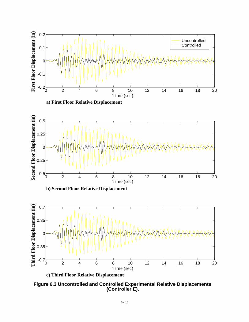
6 - 10

0 2 4 6 8 10 12 14 16 18 20-0.7

-0.35

0

0.35

0.7

0 2 4 6 8 10 12 14 16 18 20-0.5

-0.25

0

0.25

0.5

UncontrolledControlled

0 2 4 6 8 10 12 14 16 18 20-0.2

-0.1

0

0.1

0.2

Figure 6.3 Uncontrolled and Controlled Experimental Relative Displacements (Controller E).

Time (sec)

Time (sec)

Time (sec)




Fir

st F

loor

Dis

plac

emen

t (i

n)Se

cond

Flo

or D

ispl

acem

ent

(in)

Thi

rd F

loor

Dis

plac

emen

t (i

n)

6 - 11

Figure 6.4 Uncontrolled and Controlled Experimental Absolute Accelerations (Controller E).

UncontrolledControlled

0 2 4 6 8 10 12 14 16 18 20-0.3

-0.15

0

0.15

0.3

0 2 4 6 8 10 12 14 16 18 20-0.4

-0.2

0

0.2

0.4

0 2 4 6 8 10 12 14 16 18 20-0.5

-0.25

0

0.25

0.5

Time (sec)

Time (sec)

Time (sec)




Fir

st F

loor

Acc

eler

atio

n (g

)Se

cond

Flo

or A

ccel

erat

ion

(g)

Thi

rd F

loor

Acc

eler

atio

n (g

)

6 - 12

Figure 6.6 Comparison of Uncontrolled and Controlled Transfer Functions from the Ground Acceleration to the Second Floor Relative Displacement.

Figure 6.5 Comparison of Uncontrolled and Controlled Transfer Functions from the Ground Acceleration to the First Floor Relative Displacement.

Experimental Uncontrolled

Experimental Controlled

0 2 4 6 8 10 12 14 16 18 20-40

-30

-20

-10

0

10

20

30

0 2 4 6 8 10 12 14 16 18 20-30

-20

-10

0

10

20

30

40

Frequency (Hz)

Mag

nitu

de (

dB)

Frequency (Hz)

Mag

nitu

de (

dB)

6 - 13

Figure 6.8 Comparison of Uncontrolled and Controlled Transfer Functions from the Ground Acceleration to the First Floor Absolute Acceleration.

Figure 6.7 Comparison of Uncontrolled and Controlled Transfer Functions from the Ground Acceleration to the Third Floor Relative Displacement.

0 2 4 6 8 10 12 14 16 18 20-40

-30

-20

-10

0

10

20

30

0 2 4 6 8 10 12 14 16 18 20-40

-30

-20

-10

0

10

20

30

40

50

Frequency (Hz)

Mag

nitu

de (

dB)

Frequency (Hz)

Mag

nitu

de (

dB)

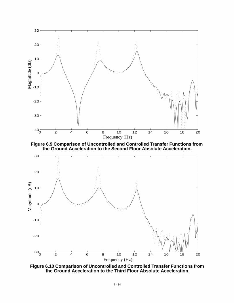
6 - 14

Figure 6.10 Comparison of Uncontrolled and Controlled Transfer Functions from the Ground Acceleration to the Third Floor Absolute Acceleration.

0 2 4 6 8 10 12 14 16 18 20-40

-30

-20

-10

0

10

20

30

0 2 4 6 8 10 12 14 16 18 20-30

-20

-10

0

10

20

30

Figure 6.9 Comparison of Uncontrolled and Controlled Transfer Functions from the Ground Acceleration to the Second Floor Absolute Acceleration.

Frequency (Hz)

Mag

nitu

de (

dB)

Frequency (Hz)

Mag

nitu

de (

dB)

6 - 15

0 2 4 6 8 10 12 14 16 18 20-0.3

-0.2

-0.1

0

0.1

0.2

0 2 4 6 8 10 12 14 16 18 20-0.4

-0.2

0

0.2

0.4


0 2 4 6 8 10 12 14 16 18 20-0.1

-0.05

0

0.05

0.1

Figure 6.11 Comparison of Experimental and Simulated Controlled Relative Displacement Responses (Controller E).

Fir

st F

loor

Dis

plac

emen

t (i

n)Se

cond

Flo

or D

ispl

acem

ent

(in)

Thi

rd F

loor

Dis

plac

emen

t (i

n)

Time (sec)

Time (sec)

Time (sec)




6 - 16


0 2 4 6 8 10 12 14 16 18 20-0.2

-0.1

0

0.1

0.2

0 2 4 6 8 10 12 14 16 18 20-0.2

-0.1

0

0.1

0.2

0 2 4 6 8 10 12 14 16 18 20-0.3

-0.15

0

0.15

0.3

Figure 6.12 Comparison of Experimental and Simulated Controlled Absolute Acceleration Responses (Controller E).

Time (sec)

Time (sec)

Time (sec)




Fir

st F

loor

Acc

eler

atio

n (g

)Se

cond

Flo

or A

ccel

erat

ion

(g)

Thi

rd F

loor

Acc

eler

atio

n (g

)

7 - 1

SECTION 7

CONCLUSION

Active control designs based on acceleration feedback have been successfully implementedand verified on a tendon-controlled, MDOF test structure at the National Center for EarthquakeEngineering Research at SUNY, Buffalo. The effects of actuator dynamics and control-structure-interaction were incorporated into the system identification procedure. The identified ten-statemodel reproduced the experimental results well in both the frequency domain and the time do-main. Experimental results indicate that effective and robust controllers can be designed using anacceleration feedback control strategy, and full state feedback performance can be recovered.

Using /LQG control design techniques, many different controllers were designed, eachwith a different performance objective. Some controllers were designed to minimize the three rel-ative displacements of the structure while others minimized the absolute acceleration of the thirdfloor. The best control design, which was designed to minimize the third floor acceleration and in-cluded the ground acceleration as an additional measurement (Controller E), achieved a 60-68%reduction in all rms displacement and acceleration measurements. Similarly, a 55% and 53% re-duction in the peak response of the third floor displacement under the scaled El Centro earthquakeand Taft excitations, respectively, was achieved. Comparable reductions were obtained for theother peak responses. In all cases, including the ground acceleration as an additional measurementresulted in a better control system. Additionally, excellent agreement was obtained between thesimulations based on the identified analytical model and the experimental results.

By comparing the various control designs it was observed that weighting the displacementsof the structure did not effectively reduce the acceleration responses. However, by weighting theaccelerations in the control design, both the displacements and accelerations were efficiently re-duced.

H2

8 - 1

SECTION 8

REFERENCES

Antoniou, Andreas. 1993. Digital Filters: Analysis, Design, and Applications, McGraw-Hill, Inc.,New York, pp. 444–446.

Bergland, G.D. 1969. A Guided Tour of the Fast Fourier Transform. IEEE Spectrum, vol. 6, pp.41–52, July.

Bendat, J.S. and Piersol, A.G. 1980. Engineering Applications of Correlation and Spectral Analy-sis, John Wiley & Sons, Inc., New York, pp. 57-–76.

Chung, L.L., R.C. Lin, T.T. Soong & A.M. Reinhorn. 1989. Experiments on Active Control forMDOF Seismic Structures,” J. of Engrg. Mech., ASCE, Vol. 115, No. 8, pp. 1609–1627.

Dyke, S.J., B.F. Spencer Jr., P. Quast & M.K. Sain. 1993. Protective System Design: The Role ofControl-Structure Interaction. Proc. of the Int. Workshop on Structural Control, Univ. of South-ern California, pp. 100–114.

Dyke, S.J., B.F. Spencer Jr., P. Quast & M.K. Sain. 1994. The Role of Control-Structure Interac-tion in Protective System Design. J. of Engrg. Mech, ASCE (in press).

Friedlander, B. 1982. Lattice Filters for Adaptive Processing. Proc. of the IEEE, 70(3).

Harris, F.J. 1978. On the Use of Windows for Harmonic Analysis with Discrete Fourier Trans-forms. Proc. of the IEEE, 66(1), pp. 51–83.

Housner, G.W. & S.F. Masri, Eds. 1990. Proc. of the U.S. National Workshop on Structural Con-trol Research, USC Publications No. M9013, University of Southern California.

Housner, G.W. & S.F. Masri, Eds. 1993. Proc. of the Int. Workshop on Structural Control, Univ.of Southern California.

Laub, A.J. 1980. Computation of Balancing Transformations. Proc. JACC, Vol. 2, paper FA8-E.

MATLAB. 1993. The Math Works, Inc. Natick, Massachusetts.

Moore, B.C. 1981. Principal Component Analysis in Linear Systems: Controllability, Observabil-ity, and Model Reduction. IEEE Trans. on Automatic Control, pp. 26–31.

Quast, P., B.F. Spencer Jr., M.K. Sain & S.J. Dyke 1994. Microcomputer Implementation of Digi-tal Control Strategies for Structural Response Reduction. Microcomputers in Civil Engrg., (inpress).

Reinhorn, A.M., T.T. Soong, M.A. Riley, R.C. Lin, S. Aizawa, & M. Higashino, Full Scale Imple-mentation of Active Control. II: Installation and Performance., Journal of Structural Engineer-ing, ASCE, Vol. 119, No. 6, June 1993, pp. 1935–1960.

8 - 2

Schoukens, J. and R. Pintelon. 1991. Identification of Linear Systems, A Pratical Guide to Accu-rate Modeling. Pergamon Press. New York, pp. 39–49.

Soong, T.T. 1990. Active Structural Control: Theory and Practice, Longman Scientific and Tech-nical, Essex, England.

Soong, T.T., A.M. Reinhorn, Y.P. Wang, & R.C. Lin. Full Scale Implementation of Active Con-trol. I: Design and Simulation., Journal of Structural Engineering, ASCE, Vol. 117, Noveember1991, pp. 3516–3536.

Spencer Jr., B.F., J. Suhardjo & M.K. Sain. 1991. Frequency Domain Control Algorithms for Civ-il Engineering Applications. Proc. of the Int. Workshop on Tech. for Hong Kong’s InfrastructureDevelopment, Hong Kong, December 19–20, 169–178.

Spencer Jr., B.F., J. Suhardjo & M.K. Sain. 1994a. Frequency Domain Optimal Control Strategiesfor Aseismic Protection. J. of Engrg. Mech, ASCE, Vol. 120, No. 1, pp. 135–159.

Spencer Jr., B.F., P. Quast., S.J. Dyke & M.K. Sain. 1994b. Digital Signal Processing Techniquesfor Active Structural Control. Proc. of the 1994 ASCE Structures Congress, Atlanta, Georgia.

Spencer Jr., B.F., M.K. Sain, C.-H. Won, D. Kaspari, Jr., & P.M. Sain 1994c. Reliability-BasedMeasures of Structural Control Robustness. Structural Safety, (in press).

Suhardjo, J. 1990. Frequency Domain Techniques for Control of Civil Engineering Structureswith Some Robustness Considerations, Ph.D. Dissertation, Univ. of Notre Dame, Dept. of CivilEngineering.

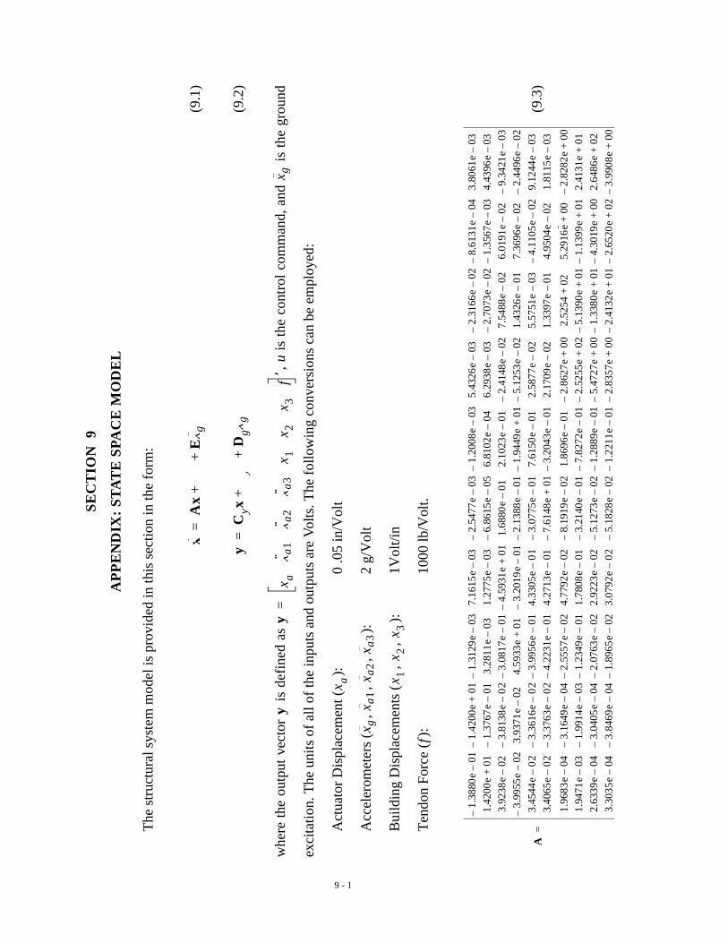
9 - 1

SE

CT

ION

9

AP

PE

ND

IX:

STA

TE

SPA

CE

MO

DE

L

The

str

uctu

ral s

yste

m m

odel

is p

rovi

ded

in th

is s

ectio

n in

the

form

:

(9.1

)

(9.2

)

whe

re t

he o

utpu

t ve

ctor

i

s de

fine

d as

,

u is

the

con

trol

com

man

d, a

nd

is

the

grou

nd

exci

tati

on. T

he u

nits

of

all o

f th

e in

puts

and

out

puts

are

Vol

ts. T

he f

ollo

win

g co

nver

sion

s ca

n be

em

ploy

ed:

Act

uato

r D

ispl

acem

ent (

):

0 .0

5 in

/Vol

t

Acc

eler

omet

ers

(,

, ,

):

2 g/

Vol

t

Bui

ldin

g D

ispl

acem

ents

(,

, ):

1V

olt/i

n

Ten

don

Forc

e (

):

1000

lb/V

olt.

(9.3

)

x·A

xB

uE

x·· g+

+=

yC

yxD

yuD

gx·· g

++

=

yy

x ax·· a

1x·· a

2x·· a

3x 1

x 2x 3

f′

=x·· g

x a

x·· gx·· a

1x·· a

2x·· a

3

x 1x 2

x 3

f

A

1.38

80e

–01

–1.

4200

e–

01+

1.31

29e

–03

–7.

1615

e03

–2.

5477

e–

03–

1.20

08e

–03

–5.

4326

e03

–2.

3166

e–

02–

8.61

31e

–04

–3.

8061

e03

–

1.42

00e

01+

1.37

67e

–01

–3.

2811

e03

–1.

2775

e03

–6.

8615

e–

05–

6.81

02e

04–

6.29

38e

03–

2.70

73e

–02

–1.

3567

e–

03–

4.43

96e

03–

3.92

38e

02–

3.81

38e

–0

2–

3.08

17e

–01

–4.

5931

e–

01+

1.68

80e

01–

2.10

23e

01–

2.41

48e

–02

–7.

5488

e02

–6.

0191

e02

–9.

3421

e–

03–

3.99

55e

–02

–3.

9371

e02

–4.

5933

e01

+3.

2019

e–

01–

2.13

88e

–01

–1.

9449

e–

01+

5.12

53e

–02

–1.

4326

e01

–7.

3696

e02

–2.

4496

e–

02–

3.45

44e

02

–3.

3616

e–

02

–3.

9956

e–

01–

4.33

05e

01–

3.07

75e

–01

–7.

6150

e01

–2.

5877

e02

–5.

5751

e03

–4.

1105

e–

02–

9.12

44e

03–

3.40

65e

02

–3.

3763

e–

02

–4.

2231

e–

01–

4.27

13e

01–

7.61

48e

–01

+3.

2043

e–

01–

2.17

09e

02–

1.33

97e

01–

4.95

04e

02–

1.81

15e

03–

1.96

83e

04–

3.16

49e

–04

–2.

5557

e–

02–

4.77

92e

02–

8.19

19e

–02

–1.

8696

e01

–2.

8627

e–

00+

2.52

5402

+5.

2916

e00

+2.

8282

e–

00+

1.94

71e

03–

1.99

14e

–03

–1.

2349

e–

01–

1.78

08e

01–

3.21

40e

–01

–7.

8272

e–

01–

2.52

55e

–02

+5.

1390

e–

01+

1.13

99e

–01

+2.

4131

e01

+

2.63

39e

04–

3.04

05e

–04

–2.

0763

e–

02–

2.92

23e

02–

5.12

73e

–02

–1.

2889

e–

01–

5.47

27e

–00

+1.

3380

e–

01+

4.30

19e

–00

+2.

6486

e02

+

3.30

35e

04–

3.84

69e

–04

–1.

8965

e–

02–

3.07

92e

02–

5.18

28e

–02

–1.

2211

e–

01–

2.83

57e

–00

+2.

4132

e–

01+

2.65

20e

–02

+3.

9908

e–

00+

=

9 - 2

(9.1

)

(9.2

)

(9.3

)

B

6.62

51e

–02

–

7.58

39e

02–

2.86

84e

01–

4.51

86e

–01

–

3.65

84e

01–

8.63

95e

01–

4.18

44e

00+

1.68

99e

01+

2.82

60e

00+

2.68

13e

00+

=

E

6.33

55e

–00

+6.

2056

e00

+

3.86

38e

00+

3.95

90e

–00

+

3.42

98e

00+

3.39

80e

00+

2.21

31e

–02

–

5.98

83e

03–

3.68

45e

–03

–

5.27

07e

03–

=

Cy

8.84

82e

–01

–1.

0256

e–

00+

4.10

46e

01–

6.15

65e

01–

1.64

89e

01–

1.86

75e

–01

–4.

1676

e00

+1.

6830

e–

01+

2.61

09e

–00

+2.

6702

e00

+

4.12

12e

–01

–4.

0830

e–

01–

2.56

94e

00+

2.49

21e

00+

2.39

08e

00+

2.38

03e

–00

+3.

5009

e–

01–

1.50

32e

00+

2.29

74e

01–

2.36

13e

–01

–

1.00

67e

–00

+1.

0149

e–

00+

1.81

11e

00+

1.85

71e

00+

2.30

79e

–0

0+

2.42

23e

00+

1.66

60e

03–

3.69

38e

–02

–6.

4788

e03

–2.

0946

e02

–

1.47

85e

–00

+1.

5234

e–

00+

1.85

73e

–00

+1.

8816

e–

00+

6.96

17e

01–

7.42

51e

–01

–1.

3385

e–

01–

1.88

72e

–01

–1.

0562

e00

+5.

6696

e02

–

1.36

29e

–00

+1.

3797

e–

00+

1.06

62e

00+

1.06

41e

00

+3.

9198

e01

–3.

9045

e–

01–

8.05

77e

–04

–1.

6463

e02

–5.

5993

e–

03–

8.95

81e

–03

–

4.13

31e

–00

+3.

6623

e–

00+

5.13

83e

01–

1.09

86e

00+

4.97

77e

–0

1–

1.98

69e

01–

6.64

40e

03–

1.10

32e

–02

–2.

8659

e–

03–

7.02

13e

–03

–

5.45

67e

–00

+5.

5829

e–

00+

7.19

50e

–0

1–

7.32

34e

–0

1–

1.29

78e

01–

1.43

61e

–01

–3.

9679

e03

–2.

1299

e02

–3.

4121

e02

–1.

3934

e02

–

9.65

68e

–00

+9.

6970

e–

00+

7.72

46e

00+

7.58

49e

00+

2.83

16e

00+

2.80

69e

–00

+2.

5274

e–

00+

1.03

06e

01+

1.53

77e

00+

1.68

25e

–00

+

=

9 - 3

(9.4

)

(9.5

)

A M

AT

LA

B f

ile c

onta

inin

g th

is m

odel

can

be

requ

este

d by

con

tact

ing

Prof

. B.F

. Spe

ncer

thro

ugh

e-m

ail a

t spe

ncer

.1@

nd.e

du.

Dy

4.51

94e

01–

3.93

46e

–02

–

2.40

50e

–03

–

8.17

83e

–04

–

4.36

86e

04–

8.92

32e

04–

3.91

45e

–03

–

2.70

16e

–01

–

=

Dg

2.14

21e

–02

–

4.41

46e·

04–

3.86

14e

04–

2.09

67e

–04

–

3.43

37e

04–

1.41

26e

04–

2.58

7104

–

1.55

28e

02–

=

EXPERIMENTAL VERIFICATION OF ACCELERATION FEEDBACK CONTROL ... · EXPERIMENTAL VERIFICATION OF...

Documents

Transcript of EXPERIMENTAL VERIFICATION OF ACCELERATION FEEDBACK CONTROL ... · EXPERIMENTAL VERIFICATION OF...