Experimental Study of Built-up-edge Formation in Micro Milling

EXPERIMENTAL STUDY OF BUILT-UP-EDGE FORMATION IN MICRO

MILLING

A Thesis

by

VIVEKANANDA REDDY KOVVURI

Submitted to the Office of Graduate and Professional Studies of

Texas A&M University

in partial fulfillment of the requirements for the degree of

MASTER OF SCIENCE

Chair of Committee, Satish Bukkapatnam

Co-Chair of Committee, Wayne N.P. Hung

Amarnath Banerjee Committee Member, Head of Department, César O. Malavé

August 2015

Major Subject: Industrial Engineering

Copyright 2015 Vivekananda Reddy Kovvuri

ii

ABSTRACT

Micromachining relies on precise tool geometry for effective material removal and

acceptable surface finish. The detrimental built-up-edges (BUEs) not only degrade the

surface finish of machined features, but also pose a concern for critical applications when

BUE can be eventually detached from machined surface.

This work presents experimental study on conditions for BUE formation and its

effects in micro milling of biocompatible 316L stainless steel. Surface finish and BUE

density on a micro milled surface are used to quantify the presence of BUE. A new micro

tool is used for each milling condition. A BUE, embedded onto a milled surface, is

identified by scanning electron microscopy and energy dispersive X-ray analysis. Optical

microscopy is used to quantify BUE density at different locations and milling parameters.

Surface finish data from meso-scale milling agree with predicted surface finish,

but the model fails to predict the surface finish in micro-scale milling. Micro milling

resulted in rough surface finish at low cutting speeds and chip loads due to formation and

detachment of BUE from tool surface to machined surface. Hence a new surface finish

model including the effect of BUE and tool wear was developed.

iii

DEDICATION

To my Mom, Dad and Brother for their love and support

iv

ACKNOWLEDGEMENTS

I would like to thank my committee chair and co-chair, Dr. Bukkapatnam and Dr.

Hung who have been constantly advising me throughout my research. They have always

guided me when required and played a critical role in my progress. I would also like to

extend my heartfelt thanks to committee member Dr. Banerjee for his constant support.

Thanks also extend to Dr. Srinivasa for his advice and suggestions.

I would like to extend a warm thanks to Zimo Wang for his guidance and assistance

in machining experiments. Thanks also go to the rest of the Smart Manufacturing Research

Group for their valuable support during this time.

I would like to thank Mr. Adam Farmer for his support and advice on machining

experiments. Thanks to HAAS Automation, Performance Micro Tools and UNIST for

providing us with valuable tools required for this research. Thanks also extend to National

Science foundation (NSF grant: CMMI 1432914, CMMI 1437319) for their support

towards this project.

Finally, thanks to my mother and father, family and friends for their

encouragement, patience and support.

v

NOMENCLATURE

α Concavity angle (o)

β Axial relief angle (o)

µ Coefficient of friction

D Tool diameter (mm)

d Depth of cut (µm)

f Chip load (µm/tooth)

δ Friction angle (o)

ϕ End rake angle (o)

θ Shear plane angle (o)

fz Spindle frequency (Hz)

Fc Cutting force (Newton)

Fs Shearing force (Newton)

h uncut chip thickness (µm)

hm Minimum chip thickness (µm)

N Tool rotational speed (revolutions per minute)

Ra Average line roughness (µm)

Rmax Maximum height of surface (µm)

re Tool edge radius (µm)

rr Ratio of uncut chip thickness to tool edge radius

Sa Average surface roughness (µm)

vi

t Maximum height of surface (µm)

v Cutting speed (m/min)

µEDM Micro-electro discharge machining

BUE Built-up-edge

CNC Computerized numerical control

CrN Chromium Nitride

CrTiAlN Chromium Titanium Aluminum Nitride

EDS Energy dispersive X-Ray spectroscopy

FEA Finite element analysis

FFT Fast Fourier transformation

HRC Rockwell C hardness

MRR Material removal rate

SEM Scanning electron microscopy

TiAlN Titanium Aluminum Nitride

TiCN Titanium carbonitride

TiN Titanium Nitride

vii

TABLE OF CONTENTS

Page

ABSTRACT .......................................................................................................................ii

DEDICATION ................................................................................................................. iii

ACKNOWLEDGEMENTS .............................................................................................. iv

NOMENCLATURE ........................................................................................................... v

TABLE OF CONTENTS .................................................................................................vii

LIST OF FIGURES ........................................................................................................... ix

LIST OF TABLES .......................................................................................................... xiv

1. INTRODUCTION .......................................................................................................... 1

1.1 Issues with non-traditional micro manufacturing techniques .......................... 3

2. OBJECTIVE AND SCOPE ........................................................................................... 5

3. LITERATURE REVIEW ............................................................................................... 6

3.1 Machining variables in micro machining ......................................................... 6

3.2 Surface finish modeling ................................................................................... 9 3.3 Built-up-edge mechanism and effects ............................................................ 18

3.4 Study of tool vibration on surface topography ............................................... 22

4. EXPERIMENTS .......................................................................................................... 24

4.1 List of equipment ........................................................................................... 24 4.2 Equipment calibrations ................................................................................... 24

4.3 Experiments .................................................................................................... 26

5. RESULTS AND DISCUSSION .................................................................................. 42

5.1 Tool runout results ......................................................................................... 42 5.2 Tool offset ...................................................................................................... 48 5.3 Detection of built-up-edge ............................................................................. 49 5.4 Surface roughness and built-up-edge ............................................................. 52 5.5 Theoretical model ........................................................................................... 55

viii

Page

5.6 Results of meso milling experiments ............................................................. 56 5.7 Results of micro milling experiments ............................................................ 62

6. CONCLUSIONS .......................................................................................................... 85

7. RECOMMENDATIONS AND FUTURE WORK ...................................................... 86

REFERENCES ................................................................................................................. 87

APPENDIX A SPECIFICATIONS OF EQUIPMENT ................................................... 91

APPENDIX B MODELLING OF LINE SURFACE ROUGHNESS IN FLAT END MILLING ......................................................................................................................... 98

APPENDIX C CNC CODE............................................................................................ 102

C.1 Spindle warmup program ............................................................................ 102 C.2 Meso and Micro slot milling program ......................................................... 102

APPENDIX D EXPERIMENTAL DATA..................................................................... 103

APPENDIX E R STATISTICAL DATA ....................................................................... 108

ix

LIST OF FIGURES

Page

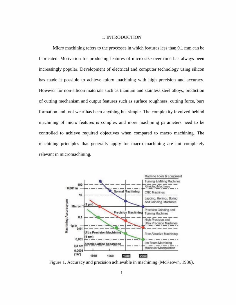
Figure 1. Accuracy and precision achievable in machining (McKeown, 1986). ............... 1

Figure 2. Small statue created by ball end micro milling using a 5-axis machine

(Sasaki et al. 2004). ............................................................................................ 2

Figure 3. Profile of micro channel with aspect ratio1.1:1, AlTiN coated WC ball end

mill, Φ0.198mm, 0.1µm/tooth chip load, 24m/min speed, 30µm depth,

316L stainless steel, MQL (Dmytro, 2013). ....................................................... 3

Figure 4. a) Macro machining where h>re b) Micro machining where h<re, re=radius

of cutting edge, h=uncut chip thickness, α=effective rake angle

(Aramcharoen and Mativenga, 2009). ................................................................ 8

Figure 5. A static model of chip formation in micro scale milling, re=radius of cutting

edge, h=uncut chip thickness, hm=minimum chip thickness (Aramcharoen

and Mativenga, 2009). ........................................................................................ 8

Figure 6. Surface profile of channel formed after ball end milling (Dmytro, 2013)........ 10

Figure 7. Surface profile generated by a two flute end mill cutter (Wang and Chang,

2004). ................................................................................................................ 11

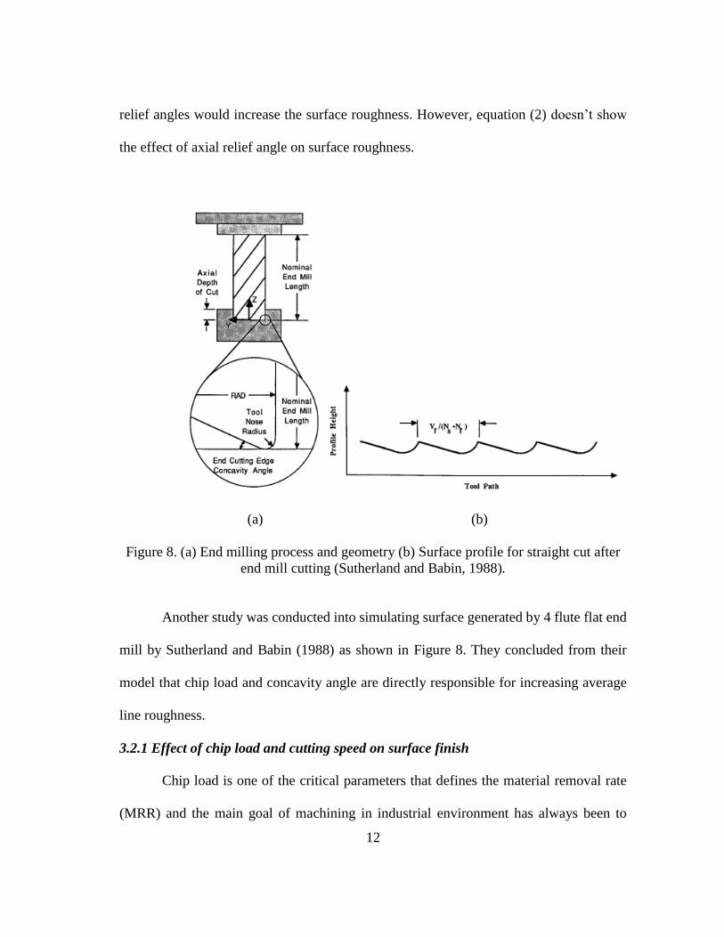
Figure 8. (a) End milling process and geometry (b) Surface profile for straight cut

after end mill cutting (Sutherland and Babin, 1988). ....................................... 12

Figure 9. Comparison of line roughness measurements and predictions for ferrite

(Vogler et al., 2004). ......................................................................................... 13

Figure 10. Relation between chip load and line roughness (Dmytro, 2013). ................... 14

Figure 11. Surface roughness variation with ratio of underformed/uncut chip

thickness to cutting edge radius (rr) (Aramcharoen and Mativenga, 2009) ...... 15

Figure 12. Dependence of roughness (Rz) with respect to cutting speed (Weule et al.,

2001). ................................................................................................................ 15

Figure 13. Percent increase in tool edge radius for coated and uncoated WC tools

(Aramcharoen et al., 2008) ............................................................................... 17

Figure 14. Comparison of surface finish for uncoated and coated tools, Lc = length of

cut (Aramcharoen et al., 2008). ........................................................................ 18

x

Page

Figure 15. SEM images showing growth of BUE at time t=0s, t=15s and t=30s at a

test temperature of 450oC, Magnification 420x (Iwata and Ueda, 1980). ........ 21

Figure 16. Cutting speed vs force per unit width (Childs, 2011). .................................... 22

Figure 17. Effect of tool vibration on surface topography (a) vibration amplitude:

0µm (b) vibration amplitude: 1µm (c) vibration amplitude: 5 µm (d)

vibration amplitude: 15 µm (Peng et al., 2012) ................................................ 23

Figure 18. Comparison of machined channel with and without runout (Sujeev, 2009). . 25

Figure 19. Experimental setup for runout measurements and milling experiments. ........ 25

Figure 20. Side view of uncoated micro flat end mill showing concavity angle. ............ 28

Figure 21. Sketch of sectional view of slot after micro milling with flat end mill.

re=radius of cutting edge ................................................................................... 28

Figure 22. Schematic diagram (side view) of workpiece preparation. ............................. 32

Figure 23. Precision gage block (thickness=3.81mm) with copper strip hanging with

support of double side sticky tape. ................................................................... 33

Figure 24. Schematic diagram representing precision gage block and Cu strip

thickness measurements with Keyence laser displacement sensor. .................. 33

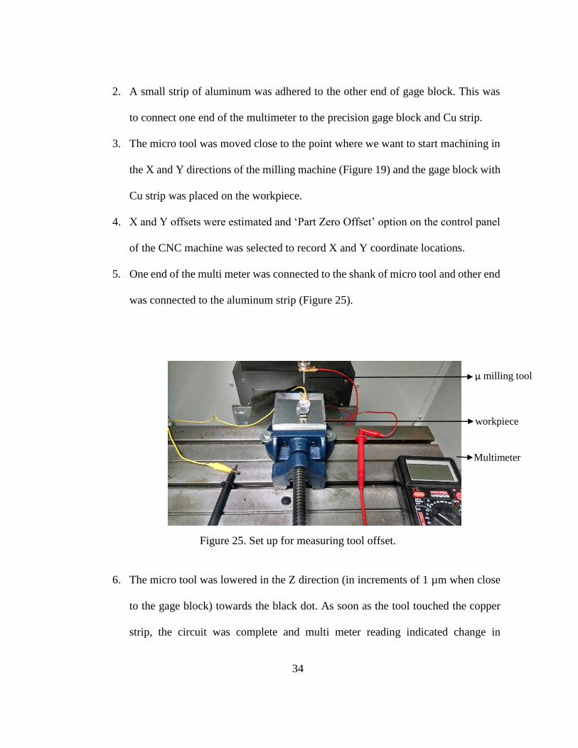
Figure 25. Set up for measuring tool offset. ..................................................................... 34

Figure 26. Time series plot at different tool rotation speeds (a) 10,000 RPM. (b)

20,000 RPM. (c) 30,000 RPM. (d) 40,000 RPM. (e) 50,000 RPM. ................. 42

Figure 27. Frequency domain plot at different tool rotational speeds (a) 10,000 RPM.

(b) 20,000 RPM. (c) 30,000 RPM. (d) 40,000 RPM. (e) 50,000 RPM. ........... 46

Figure 28. Repeatability and consistency of tool offset values. ....................................... 49

Figure 29. Tool rake surface of uncoated WC after machining 4 slots, length 32 mm,

Uncoated Φ0.406 mm WC flat end mill, 15-80 m/min speed, 15 µm/tooth

chip load, 100 µm depth, dry and MQL, A36 carbon steel workpiece. ............ 50

Figure 30. Scanning electron microscopy image of chips collected after machining

pure titanium, Uncoated WC tool, Φ0.406 mm, 2 flute, 10 m/min speed, 0.2

µm/tooth chip load, 10 µm depth, dry. ............................................................. 51

xi

Page

Figure 31. Machined surface of 316L stainless steel with uncoated WC tool, Φ0.406

mm, 2 flute, 10 m/min speed, 0.05 µm/tooth chip load, 30 µm depth, MQL. . 52

Figure 32. Linear density of BUE at center of slot, A36 carbon steel, high speed steel

tool, Φ3.175 mm, 12 mm length, 3 µm/tooth chip load, 50 µm depth, dry. ..... 53

Figure 33. Area density of BUE at center of slot, A36 carbon steel, high speed steel

tool, Φ3.175 mm, measurement area-15625 µm2, 3 µm/tooth chip load, 50

µm depth, dry. ................................................................................................... 54

Figure 34. Average line roughness at center of slot, A36 carbon steel, high speed steel

tool, Φ3.175 mm, 3 µm/tooth chip load, 50 µm depth, dry. ............................. 54

Figure 35. Predicted and actual line roughness Ra values of slots measured at center.

Al 6061-T6, high speed steel tool, Φ3.175 mm, 2 flute, 100 µm depth, dry,

3.5o concavity angle. ......................................................................................... 56

Figure 36. Average surface roughness, Sa, A36 carbon steel, uncoated and coated WC

tool, Φ3.175mm, 4 flutes, 15 µm/tooth chip load. ............................................ 58

Figure 37. (a) Uncoated WC tool before machining (b) Tool chipping and wear

observed on uncoated WC tool. Machining 4 consecutive slots, 32 mm

length, 15 m/min and 80 m/min speed, 15 µm/tooth chip load, dry and

MQL, 50 µm and 100 µm depth, A36 carbon steel. ......................................... 59

Figure 38. (a) TiAlN coated WC tool before machining (b) Tool chipping and wear

observed on TiAlN coated WC tool. Machining 4 consecutive slots, 32 mm

length, 15 m/min and 80 m/min speed, 15 µm/tooth chip load, dry and

MQL, 50 µm and 100 µm depth, A36 carbon steel. ......................................... 60

Figure 39. Built-up-edge formation observed on rake surfaces of uncoated WC tool.

Machining 4 consecutive slots, 32 mm length, 15 m/min and 80 m/min

speed, 15 µm/tooth chip load, dry and MQL, 50 µm and 100 µm depth, A36

carbon steel. ...................................................................................................... 61

Figure 40. Machined surface of A36 carbon steel. Uncoated WC tool, Φ3.175 mm, 4

flutes, 15 m/min speed, 15 µm/tooth chip load, 100 µm depth, MQL,

Sa=0.997µm. ..................................................................................................... 61


flute, 80 m/min speed, 15 µm/tooth chip load, 50 µm depth, MQL,

Sa=0.584µm. ..................................................................................................... 62

xii

Page

Figure 42. Scanning electron microscopy image of machined 316L stainless steel.

Uncoated WC micro mill, Φ0.406 mm, 10 m/min speed, 0.05 µm/tooth chip

load, 30 µm depth, MQL. ................................................................................. 63

Figure 43. Energy dispersive X-ray spectroscopy (EDS) of BUE. .................................. 63

Figure 44. BUE density showing variation for different grayscale. 27 m/min speed, 1

µm/tooth chip load, uncoated WC tool, Φ0.406 mm WC tool, 30 µm depth,

MQL. ................................................................................................................ 64

Figure 45. Grayscale image with BUE count on Image Pro software. 316L stainless

steel, 44 m/min speed, 0.5 µm/tooth chip load, uncoated WC tool, Φ0.406

mm, 30 µm depth, MQL. .................................................................................. 65

Figure 46. BUE density variation in up and down milling within a sample. 316L

stainless steel, 27 m/min speed, 1 µm/tooth chip load, uncoated WC tool,

Φ0.406 mm, 30 µm depth, MQL. ..................................................................... 66



mm, 30 µm depth, MQL, up-milling. ............................................................... 67



mm, 30 µm depth, MQL, down-milling. .......................................................... 67

Figure 49. BUE Density (average of 20 samples per slot) on micro milled slots. 316L

stainless steel, 10-60 m/min speed, 0.05-1 µm/tooth chip load, 30 µm depth,

Φ0.406 mm uncoated WC flat end mill, 2 flutes, MQL. .................................. 68

Figure 50. (a) Flat end mill showing view area of micro end mill tool. (b) Scanning

electron microscopy image of cutting edge of uncoated WC tool, Φ0.406

mm, 10 m/min speed, 0.05 µm/tooth chip load, 30 µm depth, 24 mm milling

length, MQL. .................................................................................................... 69

Figure 51. (a) Flat end mill with arrows pointing towards view area of micro end mill

tool. (b) Scanning electron microscopy image of cutting edge. Uncoated

WC tool with BUE, Φ0.406 mm, 10 m/min speed, 0.05 µm/tooth chip load,

30 µm depth, 24 mm milling length, MQL. ..................................................... 70

Figure 52. Energy dispersive X-ray spectroscopy results of BUE on tool....................... 71

xiii

Page


electron microscopy image of rake surface and cutting edge. Uncoated WC

tool with BUE, Φ0.406 mm, 60 m/min speed, 1 µm/tooth chip load, 30 µm

depth, 24 mm milling length, MQL. ................................................................. 72


electron microscopy image of rake surface and cutting edge. AlTiN WC

tool with BUE, Φ0.800 mm, 10 m/min speed, 2-8 µm/tooth chip load, 30

µm depth, 48 mm milling length, MQL. .......................................................... 73

Figure 55. Surface roughness Sa (average of 15 values) measured at center of slot.

Micro milling, 316L stainless steel, 10-60 m/min speed, 0.05-1 µm/tooth

chip load, 30 µm depth, Φ0.406 mm uncoated WC flat end mill, 2 flutes,

MQL. ................................................................................................................ 74

Figure 56. Predicted and actual line roughness, Ra values of slots measured at center.

316L stainless steel, Φ0.406 mm uncoated WC tool, 2 flute, 10-60 m/min

speed, 0.05-1 µm/tooth chip load, 30 µm depth, MQL, 7o concavity angle. .... 75

Figure 57. Predicted and actual line roughness, Ra values of slots measured at center. .. 76

Figure 58. (a) Top view of new micro tool (b) Top view of micro tool after 24 mm

milling distance, 316L stainless steel, 27 m/min speed, 1 µm/tooth chip

load, Φ0.406 mm uncoated WC tool, 30 µm depth, MQL. .............................. 77

Figure 59 (a) Top view of machined tool superimposed on top view of new micro tool

(b) One of the cutting edges magnified to calculate tool wear and chipping

after milling 24 mm, 316L stainless steel, 27 m/min speed, 1 µm/tooth chip

load, Φ0.406 mm uncoated WC tool, 30 µm depth, MQL. .............................. 77

Figure 60. Average tool volumetric loss per machining length after micro machining

slots with 10-60 m/min cutting speed, 0.05-1 µm/tooth chip load, 30 µm

depth, Φ0.406 mm uncoated WC flat end mill, 2 flutes, 316L stainless steel

workpiece. ......................................................................................................... 79

Figure 61. Average tool volumetric loss per machining time after micro machining

slots with 10-60 m/min cutting speed, 0.05-1 µm/tooth chip load, 30 µm

depth, Φ0.406 mm uncoated WC flat end mill, 2 flutes, 316L stainless steel

workpiece. ......................................................................................................... 80


316L stainless steel, Φ0.406 mm uncoated WC tool, 2 flute, 10-60 m/min

speed, 0.05-1 µm/tooth chip load, 30 µm depth, MQL, 7o concavity angle. .... 84

xiv

LIST OF TABLES

Page

Table 1. Cutting edge radius before and after coating tools (Aramcharoen et al.,

2008). ................................................................................................................ 17

Table 2. Comparison of uncoated and TiAlN coated meso end mill cutters (MSC

Industrial Supply, 2014). .................................................................................. 26

Table 3. Properties of uncoated WC micro tools (Performance Micro Tools, 2014). ..... 27

Table 4. Physical properties of workpiece materials (Azom, 2014) (Steel Grades,

2014). ................................................................................................................ 29

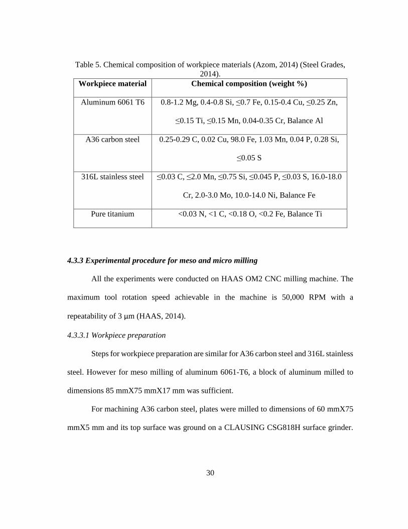
Table 5. Chemical composition of workpiece materials (Azom, 2014) (Steel Grades,

2014). ................................................................................................................ 30

Table 6. Meso milling experimental conditions. .............................................................. 37

Table 7. Micro milling experimental conditions. ............................................................. 38

Table 8. Spindle speed frequencies calculated at various tool rotational speeds. ............ 42

Table 9. Tool runout values measured at different speeds. .............................................. 45

Table 10. Correlation between Linear density of BUE, Area density of BUE and Line

roughness, Ra, A36 carbon steel, 5 m/min speed, high speed steel tool,

Φ3.175 mm, 12 mm length, 3 µm/tooth chip load, 50 µm depth, dry. ............. 53

Table 11. Preliminary linear model fit using R statistical software. ................................ 58

Table 12. Final linear model fit using R statistical software ............................................ 59

Table 13. Comparison between material composition of 316L stainless steel and BUE

(Azom, 2014) (Steel Grades, 2014). ................................................................. 64

Table 14. EDS of BUE on cutting edge, Uncoated WC tool with BUE, Φ0.406 mm,

10 m/min speed, 0.05 µm/tooth chip load, 30 µm depth, 24 mm milling

length, MQL. .................................................................................................... 71

Table 15. Tool wear and chipping for micro milling experimental conditions, 316L

stainless steel workpiece, Φ0.406 mm uncoated WC tool, MQL ..................... 78

Table 16. Final model using R statistical software for difference between predicted

roughness and actual roughness ........................................................................ 81

xv

Page


roughness and actual roughness ........................................................................ 82

1

1. INTRODUCTION

Micro machining refers to the processes in which features less than 0.1 mm can be

fabricated. Motivation for producing features of micro size over time has always been

increasingly popular. Development of electrical and computer technology using silicon

has made it possible to achieve micro machining with high precision and accuracy.

However for non-silicon materials such as titanium and stainless steel alloys, prediction

of cutting mechanism and output features such as surface roughness, cutting force, burr

formation and tool wear has been anything but simple. The complexity involved behind

machining of micro features is complex and more machining parameters need to be

controlled to achieve required objectives when compared to macro machining. The

machining principles that generally apply for macro machining are not completely

relevant in micromachining.

Figure 1. Accuracy and precision achievable in machining (McKeown, 1986).

2

Figure 1 represents manufacturing precision and accuracy curves which were first

proposed by Taniguchi (1980) and later modified McKeown (1986). With advancement

in the realm of science and technology, CNC machines with positional accuracies in the

range of a few nanometers have been developed in the early 1990’s (Byrne et al., 2003).

Complex micro part features are fabricated as their demand is on the rise owing to

increased usage in fuel injection nozzles in aerospace and automobile industries,

integrated circuit packages in semi-conductor industry, stent and drug delivery systems in

bio-medical industry (Bourne, 2007; Liu et al., 2004).

Usage of stainless steel in these applications is gaining prominence due to its

properties such as high ductility, toughness, corrosion and oxidation resistance. The goal

of micro machining is to fabricate these small features with high accuracy and precision.

Figure 2. Small statue created by ball end micro milling using a 5-axis machine (Sasaki

et al. 2004).

An example of complex part that could be fabricated is shown in Figure 2. Sasaki

et al. (2004) machined gold for 36 hours using a single crystal diamond ball end mill on a

3

5-axis machine to fabricate this statue. Also features with high aspect ratios can be

fabricated in micro milling with ease over other non-traditional fabrication methods as

shown in Figure 3 (Dmytro, 2013). Various non-traditional micro fabrication processes

are known to exist to machine these features. In this study, micro milling has been chosen

due to its flexibility in machining complex part features.

Figure 3. Profile of micro channel with aspect ratio1.1:1, AlTiN coated WC ball end

mill, Φ0.198mm, 0.1µm/tooth chip load, 24m/min speed, 30µm depth, 316L stainless

steel, MQL (Dmytro, 2013).

1.1 ISSUES WITH NON-TRADITIONAL MICRO MANUFACTURING

TECHNIQUES

Both traditional and non-traditional techniques can produce micro features.

Although many non-traditional processes have been developed to achieve the same level

of accuracy and precision as in traditional machining process, they have their own

limitations. Laser beam machining and electron beam machining can machine almost any

available material as the heat generated during the process can exceed the melting point

4

of all known materials. However the heat affected zone is difficult to control (Masuzawa,

2000).

Photo etching can specify a pattern with good precision with etching proceeding

iso-tropically, which restricts the application of this method to only semiconductor

products. (Masuzawa, 2000). Rapid prototyping techniques like stereo-lithography can

also be used in micro fabrication with major drawback being the limited availability of

materials.

Micro-electro discharge machining (µEDM) is a machining process which

removes material by melting and vaporization. High machining accuracy is easily

achieved by µEDM whereas high machining speed is yet to be reached. Although the use

of deionized water improves machining speed to an extent, it does so at the expense of

machining accuracy (Masaki et al., 1990).

Traditional methods for micro fabrication include micro milling which is an

extension of macro milling on a smaller scale. In this study, micro milling has been chosen

due to its flexibility in machining complex part features. Also features with high aspect

ratios can be fabricated using micro milling with ease over other non-traditional

fabrication methods. One of the major limitations of micro milling is the formation of

built-up-edge (BUE). The presence of BUE on the machined surface results in higher

average surface roughness values. Detection of BUE is critical so as to avoid its formation

for producing high quality micro part features. Since BUE related information is limited

in micro milling, this work is an experimental study on optimizing machining parameters

for BUE formation.

5

2. OBJECTIVE AND SCOPE

The primary objective of this study is

1. Study BUE formation in micro milling

2. Predict surface roughness and effect of BUE

3. Optimize process parameters to obtain best surface with minimum BUE

The scope of this study limits to:

1. Micro milling of 316L stainless steel using uncoated and coated tungsten carbide

flat end mill cutters with diameters less than <0.500 mm.

2. Meso milling of Aluminum 6061-T6 with high speed steel cutter.

3. Meso milling of A36 carbon steel with coated and uncoated tungsten carbide flat

end mill cutters of diameters 3 mm.

4. Applying minimum quantity lubrication through micro mist.

6

3. LITERATURE REVIEW

3.1 MACHINING VARIABLES IN MICRO MACHINING

Micro and macro machining are different in various aspects especially cutting

mechanism, chip formation, surface generation etc. The motivation and knowledge of

macro machining could be slightly extended to micro machining but cannot be completely

applied. Since the availability of relevant literature in micro machining is limited, review

of related macro machining literature is cited for reference.

3.1.1 Uncut chip thickness and edge radius

A lot of research has been done in the field of uncut chip thickness and its

significance in micro machining. Its importance has been discussed by Ikawa et al. (1992)

at length although studies have been conducted before that in 1988. Furukawa and

Moronuki (1988) observed increase in specific cutting force for aluminum alloy with

different grain sizes below cutting depths of 3 µm and reached normal standard cutting

force values at higher depths. This might be due to sliding of aluminum alloy under flank

face due to elastic recovery at small depths. They concluded that a minimum depth of cut

is required.

Ikawa et al. (1988) machined copper using a specially prepared diamond cutting

edge and produced chips in the range of 1 nm. The cutting edge sharpness was less than

1nm. They developed atomistic models to validate their claim that chips are formed only

if thickness of cut is above a critical value. They further extended their study on minimum

thickness of cut by applying molecular dynamics simulation on accuracy in micro cutting

7

which they found out to be about 1nm or less and called it minimum thickness of cut below

which a chip is not formed (Shimada et al., 1993).

Yuan et al. (1996) studied the relation between tool edge radius and minimum chip

thickness in ultra-machining of aluminum alloys with diamond coated cutting tools and

derived mathematical equations based on cutting forces to estimate minimum thickness of

cut. They found that minimum chip thickness was a function of coefficient of friction (µ)

between workpiece and tool material and estimated minimum chip thickness for different

combinations of workpiece and tool materials. They found it to be between 20-40% of

tool edge radius in cutting most of the materials.

Lai et al. (2008) used finite element models to simulate machining of Oxygen-free

high thermal conductivity (OFHC) copper with minimum chip thickness between 10-30%

of tool edge radius and observed chip formation for 30% of tool edge radius when the

cutting edge radius is around 2µm. After a series of experiments, they recommended

minimum thickness of cut for machining OFHC copper to be 25% of cutter edge radius.

Aramcharoen and Mativenga (2009) proposed a conclusive model on minimum

cut thickness with respect to tool edge radius as evident from Figures 4 and 5. They

suggested that minimum thickness of cut depends on sharpness of cutting edge and tool

workpiece material affinity. They suggested that chip formation in micro machining does

not follow the same principles of macro machining, and its formation is uncommon in

micro machining unless uncut chip thickness is greater than tool edge radius.

8

a) b)

Figure 4. a) Macro machining where h>re b) Micro machining where h<re, re=radius of

cutting edge, h=uncut chip thickness, α=effective rake angle (Aramcharoen and

Mativenga, 2009).

They proposed three cutting mechanisms in micro machining depending on uncut chip

thickness (depth of cut) h, minimum chip thickness hm and tool radius of cutting edge re.

1) h<hm<re

In Figure 5(a), the uncut chip thickness is less than tool edge radius. When this

happens, elastic deformation of workpiece takes place resulting in no chip formation. A

tool has negative rake angle which encourages the rake surface of tool to push forward the

workpiece material resulting in ploughing and no chip formation (Aramcharoen and

Mativenga, 2009).

a) h<hm<re b) h=hm=re c) h>hm>re

Figure 5. A static model of chip formation in micro scale milling, re=radius of cutting

edge, h=uncut chip thickness, hm=minimum chip thickness (Aramcharoen and

Mativenga, 2009).

9

2) h=hm=re

As this uncut chip thickness value increases and equals tool edge radius as shown

in Figure 5(b), plastic deformation dominates over elastic deformation. Transition from

ploughing or elastic deformation to cutting or plastic deformation is observed

accompanied by chip formation.

3) h>hm>re

As the uncut chip thickness is greater than tool edge radius, plastic deformation of

workpiece material or chip formation is observed. (Figure 5(c)).

3.2 SURFACE FINISH MODELING

In most of the research concerning optimizing surface finish, a surface model is

either derived mathematically or simulated to predict average roughness values. These

values are then compared with actual values obtained, and deviation from predicted

average roughness is calculated and explained. To achieve the best possible finish,

different combination of machining parameters are tried to find the best combination that

results in small values of average surface roughness (Sa).

Dmytro (2013) predicted line roughness at the center of slot for micro ball end

milling under the assumptions that depth of cut was large enough to avoid ploughing and

cutting tool edge was sharp. Finished surface model was developed to predict line

roughness shown in Figure 6 and equation (1). This model predicts line roughness

reasonably well, when the chip load is above 50 µm/tooth.

10

Figure 6. Surface profile of channel formed after ball end milling (Dmytro, 2013).

(1)

where Ra = Line roughness (mm)

f = Chip load (mm/tooth)

D = Diameter of tool (mm)

Wang and Chang (2004) simulated surface generated by 2 flute flat end mills

(Figure 7). They conducted experiments with 5 factors, each at 5 levels, including cutting

speed, chip load, depth of cut, concavity angle and axial relief angle to verify their

mathematical equation (2).

11

Figure 7. Surface profile generated by a two flute end mill cutter (Wang and Chang,

2004).

Ra = 𝑓

4 𝑐𝑜𝑡𝛾 (2)

where Ra = Line roughness (mm)

Rmax = Maximum height of surface (mm)

f = Chip load (mm/tooth)

𝛾 = Concavity angle (o)

β = Axial relief angle (o)

Using response surface methodology (RSM) and experimental analysis, Wang and

Chang (2004) found that for dry cutting, significant parameters affecting average

roughness were cutting speed, chip load, concavity and axial relief angles. For wet cutting,

chip load and concavity angles were the critical parameters. They found that, when the

concavity angle is greater than 2.50, an increase in chip load, concavity angle and axial

β

12

relief angles would increase the surface roughness. However, equation (2) doesn’t show

the effect of axial relief angle on surface roughness.

(a) (b)

Figure 8. (a) End milling process and geometry (b) Surface profile for straight cut after

end mill cutting (Sutherland and Babin, 1988).

Another study was conducted into simulating surface generated by 4 flute flat end

mill by Sutherland and Babin (1988) as shown in Figure 8. They concluded from their

model that chip load and concavity angle are directly responsible for increasing average

line roughness.

3.2.1 Effect of chip load and cutting speed on surface finish

Chip load is one of the critical parameters that defines the material removal rate

(MRR) and the main goal of machining in industrial environment has always been to

13

achieve a high MRR. Cui et al. (2012) machined AISI H13 steel with a tool diameter of

125 mm with tungsten carbide inserts and found that chip load is directly proportional to

surface roughness. In a study by Zawawi et al. (2014) on machining aluminum and P20

steel with a 12 mm diameter end mill, they found that surface roughness deteriorates by

increasing chip loads. However, in micro machining, there has always been a debate on

the effect of chip load on surface finish.

Vogler et al. (2004) micro milled ferrite and pearlite at chip loads from 0.25-3

µm/tooth, spindle speed of 120000 RPM, and with axial depth of cuts at 50 µm and 100

µm. They observed that a chip load of 3.0 µm/tooth has a lower line roughness compared

to a chip load of 0.25 µm/tooth (Figure 9). They compared their experimental results with

predicted results using finite element analysis and found the prediction to be in close

agreement.

Figure 9. Comparison of line roughness measurements and predictions for ferrite (Vogler

et al., 2004).

14

However, another study conducted by Dmytro (2013) on micromachining of ball

end mills of 316L Stainless steel and Ni-Ti alloys shows that surface roughness increases

with chip load. It is clearly evident from Figure 10 that increase in chip load with a

constant cutter diameter, resulted in higher average line roughness.

Figure 10. Relation between chip load and line roughness (Dmytro, 2013).

Another important study on uncut chip thickness and surface finish was done by

Aramcharoen and Mativenga (2009) in which they machined H13 hardened steel at

different ratios of uncut chip thickness to tool edge radius (rr) as shown in Figure 11.

15

Figure 11. Surface roughness variation with ratio of underformed/uncut chip thickness to

cutting edge radius (rr) (Aramcharoen and Mativenga, 2009)

They based their study on 3 different cases.

1. rr < 1, the surface roughness values decreases with increase in chip load as

observed by Vogler et al., (2004).

2. rr > 1, chip load has a positive correlation with surface roughness. This study is in

acceptance with the study conducted by Dmytro (2013) on micromachining of

stainless steel using ball end mills.

3. rr = 1, the best surface finish occurs.

Figure 12. Dependence of roughness (Rz) with respect to cutting speed (Weule et al.,

2001).

re>fz

re<fz

re=fz

16

Weule et al., (2001) milled SAE 1045 steel with cutting velocities ranging from 5

m/min to 420 m/min. Chip load, depth of cut and type of cutting (up and down milling)

were other variable parameters. They found that surface roughness decreases with increase

in cutting velocity except for a small region (around 1-60 m/min) (Figure 12). This

suggests the possibility of BUE formation on the rake surface of tool at these cutting

speeds.

3.3.2 Tool coatings

Coatings (both soft and hard) on tungsten carbide tools have been effectively and

efficiently used in macro machining till date with fair amount of decrease in cutting forces

and surface finish. Tool coatings protect the cutting edge by forming an extra layer over

rake surface and cutting edges and thus protecting the cutting edge from wear, resulting

in longer tool life. Also depending upon the type of tool coating used, coefficient of

friction between the coating material and workpiece material would be reduced, thereby

ensuring reduced friction and temperatures at tool chip interface.

Aramchareon et al. (2008) studied the effect of hard coatings in micro milling of

hardened H13 tool steel (45 HRC) using flat end mills under dry conditions. They

evaluated effect of TiN, TiCN, TiAlN, CrN and CrTiAlN coatings on tools made from

ultra-fine tungsten carbide structure. Also coating effectively increases the tool edge

radius by almost 2 times. Details of cutting edge radius before and after for different types

of coating are provided in Table 1. For most of micro cutting applications coating

thickness is in the range of 1.5+0.15 µm. The cutting edge radius before and after coating

was measured on a scanning electron microscope (SEM).

17

Table 1. Cutting edge radius before and after coating tools (Aramcharoen et al., 2008).

Figure 13. Percent increase in tool edge radius for coated and uncoated WC tools

(Aramcharoen et al., 2008)

Figure 13 shows cutting edge radius enlargement after machining hardened H13

tool steel for a length of cut (Lc) of 20-25 mm. Overall, coated micro end mills perform

better than uncoated tools due to improved friction characteristics at workpiece tool

interface. Among coated tools TiN coating performs best in terms of percentage

enlargement of cutting edge radius.

18

Figure 14. Comparison of surface finish for uncoated and coated tools, Lc = length of cut

(Aramcharoen et al., 2008).

Figure 14 compares surface finish at the beginning of slot and after machining a

length of 20-25 mm with both coated and uncoated tools. CrN tool initially shows promise

of better performance over all other tools, but slowly deteriorates upon time. At the end of

20-25 mm length, surface finish of uncoated, TiCN and CrN tools are poor due to large

flank wear and delamination of coating (Aramcharoen et al., 2008). However, a rationale

behind improvement in surface finish for TiN, TiAlN and CrTiAlN was not provided.

3.3 BUILT-UP-EDGE MECHANISM AND EFFECTS

Built-up-edge is a phenomenon in which the chip material welds or sticks to the

tool rake surface. This extra layer of workpiece material protects the original rake surface

from wear. It also acts as a new cutting edge covering the original cutting edge thus

modifying the tool geometry. This BUE occurs quite frequently while machining ductile

materials such as stainless steel and mainly effects cutting forces, vibrations, tool life and

surface finish. The BUE formation is dynamic in the sense that, it increases in size, breaks

19

off from the rake surface of the tool and forms again. Research on BUE formation has

always been a topic of prime interest in the realm of manufacturing.

Heginbotham and Gogia (1961) had shown that cutting speed has a major influence

on the formation of BUE. At about the same time, Zorev (1966) has reinforced that cutting

speed has significant impact on the formation of BUE and proposed that cutting speeds

for BUE formation in machining carbon steels are in the range of 1-50 m/min.

Sukvittayawong and Inasaki (1994) measured cutting force to detect BUE in

turning process. Their assumption was based on the fact that, whenever BUE was formed

on the face of the rake, the chip was no longer moving on the rake surface but on the BUE

surface. This led to a negative effective end rake angle (ϕ), resulting in higher cutting

forces from Merchants equation (Groover, 2004).

Fc= Fs * cos(𝛿−𝜙)

cos(𝜃+𝛿−𝜙) (3)

where Fc = cutting force (N)

Fs = shearing force (N)

δ = friction angle (o)

ϕ = end rake angle (o)

θ = shear plane angle (o)

As cutting speed was increased beyond a critical point, BUE breaks, resulting in

positive rake angle, decreasing cutting forces again. This cyclic process of increase and

decrease in cutting forces was used to detect formation of BUE. This increase in cutting

force, however could be attributed to other machining changes like tool wear. There was

20

no particular reason explained why this variation in cutting force occurs only due to BUE

formation.

Iwata and Ueda (1980) machined low carbon steel with high speed SKH-9 tool at

cutting speed of 0.15 mm/min and test temperatures between 350-500 oC at tool rake

surface. They proposed a complicated mechanism for formation of BUE based on SEM

images of machining observed over time (Figure 15). They observed workpiece material

to appear around the cutting edge of the tool. Consequently, they found two cracks: one

below the flank face which grows in the primary shear zone along a slip line and other

ahead of rake surface at a distance from the cutting edge. At this stage BUE becomes

clearly evident and continues to grow along these cracks. The crack growth is in the region

of severe strain concentration which starts from the current position of crack tip and

continues to grow along a slip line.

This reinforces the fact that fracture behavior of workpiece material plays a

significant role in BUE formation in addition to the adhesion property. Below 350-500oC,

there is not sufficient adhesion between workpiece and tool material to support formation

of BUE while above this range the ability of material to recover its ductility inhibits crack

formation which is necessary for BUE formation.

21

Figure 15. SEM images showing growth of BUE at time t=0s, t=15s and t=30s at a test

temperature of 450oC, Magnification 420x (Iwata and Ueda, 1980).

Formation of BUE has always been difficult to predict. A lot of research has been

done to quantify and predict BUE formation. Fang et al. (2010) used a Neural network

approach and developed Resource Allocation Network (RAN) and Multilayer Perceptron

(MLP) Network models for round and sharp cutting edges to predict BUE formation in

orthogonal machining of 2024-T351 aluminum alloy, corresponding to multitude of inputs

including cutting speed, feed rate, cutting force, thrust force and vibration amplitude.

Experiments were conducted at different extremes of speed (26 levels from 0.80-250

m/min) and feed rates (8 levels from 0.01-0.3 mm/rev). Based on input parameters they

were able to classify three stages of BUE formation. When the cutting speed was below

20 m/min, BUE formation occurred at tool rake surface and grew in size. When the cutting

speed was between 20-100 m/min, BUE formation is intermittent. At high cutting speeds,

over 100 m/min, there is no BUE formation.

Childs (2011) used finite element analysis (FEA) to simulate machining of a type

of carbon steel using cemented carbide tool at cutting speeds ranging from 1-150 m/min.

His results indicated the BUE was significant in the speed range of 1-60 m/min. Cutting

22

force and thrust force per unit width were used to compare BUE formation for different

speed ranges (Figure 16). Simulation results showed that BUE was observed when the

temperature range at the rake chip interface was between 300-500oC, which agreed with

study from Iwata and Ueda (1980).

Figure 16. Cutting speed vs force per unit width (Childs, 2011).

Shahabi and Ratnam (2010) proposed an on-site inspection technique to detect and

measure BUE using machine vision approach. They used subtraction method and polar-

radius transformation algorithms on images captured by a high resolution CCD camera to

detect BUE. Actual images of tools before and after cutting are aligned and image of tool

before cutting is subtracted from image of tool after cutting, to find area of BUE. They

found both the methods to perform within a mean difference of 6.5%.

3.4 STUDY OF TOOL VIBRATION ON SURFACE TOPOGRAPHY

Tool vibration is an inseparable phenomenon present and has a direct influence on

the final surface produced especially when the tool vibration and surface finish are in the

23

same scale. Peng et al. (2012) simulated surfaces by using a 1mm diameter ball end mill,

with a constant chip load of 80 µm/tooth, spindle speed of 7500 RPM and tool radius of

0.5 mm. They found that with increase in vibration amplitude, average surface roughness

increases from 0.76 µm without vibration to 3.4 µm with vibration of 15 µm (Figure 17).

(a) (b)

(c) (d)

Figure 17. Effect of tool vibration on surface topography (a) vibration amplitude: 0µm

(b) vibration amplitude: 1µm (c) vibration amplitude: 5 µm (d) vibration amplitude: 15

µm (Peng et al., 2012).

Y, µm

X, µm

Z, µm

X, µm

Y, µm

Z, µm

X, mm

Y, mm

Z, µm

Y, mm

X, mm

Z, µm

24

4. EXPERIMENTS

4.1 LIST OF EQUIPMENT

A variety of equipment have been used throughout the experimentation phase.

These equipment can be broadly classified into machining equipment, data collection

equipment and metrology equipment. A brief introduction on machines and their usage is

described in the experiment section. A detailed list of specifications is provided in

Appendix A.

1. HAAS OM2 milling machine

2. CLAUSING CSG818H Surface Grinder

3. UNIST lubrication system

4. KEYENCE laser displacement sensor (LK-G series)

5. OLYMPUS optical microscope

6. ZYGO ZeGage 3D optical surface profiler

7. TESCAN Vega LM3

8. UNI-T M890G digital multimeter

9. Metason 200 ultrasonic cleaner

4.2 EQUIPMENT CALIBRATIONS

4.2.1 Runout measurements

Tool runout in simple terms is imperfect alignment of tool in the spindle. Presence

of tool runout cuts unequal quantities of material by each tooth. Tool runout is considered

negligible in macro machining since runout is very small compared to slot width. However

25

in micro machining it is highly significant as tool runout is comparable to the slot width

and hence even a small value of runout can result in inaccurate slot widths (Figure 18).

Figure 18. Comparison of machined channel with and without runout (Sujeev, 2009).

Figure 19. Experimental setup for runout measurements and milling experiments.

MQL nozzle

Laser

workpiece

X

Z

26

Keyence laser displacement sensor was used to measure tool runout. It was

mounted on a rigid stand, independent of machine frame (Figure 19). Fast Fourier

Transformations (FFT) were used to obtain frequency domain graphs to analyze the

components of output signal. The time domain and frequency graphs were plotted in

MATLAB. A Φ3.175mm plug gage was used to measure tool runout at tool rotational

speeds ranging from 10,000-50,000 RPM in uniform increments of 10,000 RPM.

4.3 EXPERIMENTS

4.3.1 Tool specifications

Two sizes of milling cutters were used for the experiments. Uncoated high speed

steel tool with tool diameter of 3.175 mm was used for machining aluminum 6061-T6.

Coated and uncoated tungsten carbide (WC) flat end mills with tool diameter of 3.175 mm

were used for meso milling experiments with A36 carbon steel (Table 2).

Table 2. Comparison of uncoated and TiAlN coated meso end mill cutters (MSC

Industrial Supply, 2014).

Tool material High speed steel Tungsten carbide Tungsten carbide

Type of coating Uncoated Uncoated TiAlN

Number of flutes 2 4 4

Cutter diameter, mm 3.175 3.175 3.175

Shank diameter, mm 3.175 3.175 3.175

Cutter length, mm 15.830 15.830 8.830

Tool length, mm 38.320 38.320 38.320

Concavity angle

(average of 10

measurements per

flute, 2 flutes per

tool)

3.5o 6.2o 11.5o

Standard deviation

of concavity angle

0.15o 0.13o 0.22o

27

Micro flat end mills were used to mill 316L stainless steel. The diameter of these

tools were 0.406 mm (TS-2-0160-S). A detailed list of tool specifications and properties

is given in Table 3.

Table 3. Properties of uncoated WC micro tools (Performance Micro Tools, 2014).

Tool material µ grained tungsten

carbide in Co matrix

µ grained tungsten Type of coating uncoated AlTiN coated

Number of flutes 2 1

Cutter diameter, mm 0.406 0.8

Shank diameter, mm 3.175 3.175

Flute length, mm 0.6096 11

Tool length, mm 38.1 38.1

Concavity angle 7o 5.2o

Cutting edge radius, re, µm

(Average of 10 measurements on

both sides of machined slot)

2.21 3.6

The concavity angle for meso tools was measured using the Olympus optical

microscope. The tool holder was placed along the Y-axis of the optical microscope table.

A rectangle box was used as a reference to measure the angle accurately (Figure 20). The

angle measurement was done using the measurement features in the embedded optical

microscope software. However, the concavity angle for a micro tool was obtained from

the tool manufacturer (Performance Micro Tools, 2014).

28

Figure 20. Side view of uncoated micro flat end mill showing concavity angle.

Figure 21. Sketch of sectional view of slot after micro milling with flat end mill.

re=radius of cutting edge

Figure 21 shows cross sectional view of slot after machining with a micro end mill.

Since the tool geometry is replicated on the slot, measurement of radius of cutting edge

(re) was done at the beginning of the slot, as the tool remains new at the beginning.

+ re

29

4.3.2 Workpiece material properties

Three different materials were chosen to conduct experiments.

Aluminum 6061 T6 was initially machined on meso scale using high speed steel

tool (Φ3.175 mm) to validate the theoretically derived average line roughness

equation.

A36 carbon steel was chosen to conduct experiments on meso scale with tungsten

carbide tools (Φ3.175 mm) to investigate significant factors effecting the quality

of surface and BUE formation. These critical factors were later varied during

designing experiments in micro milling.

316L stainless steel material has been picked for micro milling experiments owing

to its vast application in the realm of medical applications.

The physical properties and chemical composition of the above materials can be found in

Table 4 and Table 5 respectively.

Table 4. Physical properties of workpiece materials (Azom, 2014) (Steel Grades, 2014).

Mate

rial

of

work

pie

ce

Yie

ld

stre

ngth

(MP

a)

Ult

imate

ten

sile

stre

ngth

(MP

a)

Mod

ulu

s

of

ela

stic

ity

(GP

a)

Hard

nes

s

(RB)

Den

sity

(g/c

m3)

Al-6061 260-310 207 69 95-97 2.7

A36 carbon

steel

250 400-550 200 67.0-83.0 7.85

316L stainless

steel

170 485 193 95 8.0

Pure titanium 170 240 21-69 70 6.45

30

Table 5. Chemical composition of workpiece materials (Azom, 2014) (Steel Grades,

2014).

Workpiece material Chemical composition (weight %)

Aluminum 6061 T6 0.8-1.2 Mg, 0.4-0.8 Si, ≤0.7 Fe, 0.15-0.4 Cu, ≤0.25 Zn,

≤0.15 Ti, ≤0.15 Mn, 0.04-0.35 Cr, Balance Al

A36 carbon steel 0.25-0.29 C, 0.02 Cu, 98.0 Fe, 1.03 Mn, 0.04 P, 0.28 Si,

≤0.05 S

316L stainless steel ≤0.03 C, ≤2.0 Mn, ≤0.75 Si, ≤0.045 P, ≤0.03 S, 16.0-18.0

Cr, 2.0-3.0 Mo, 10.0-14.0 Ni, Balance Fe

Pure titanium <0.03 N, <1 C, <0.18 O, <0.2 Fe, Balance Ti

4.3.3 Experimental procedure for meso and micro milling

All the experiments were conducted on HAAS OM2 CNC milling machine. The

maximum tool rotation speed achievable in the machine is 50,000 RPM with a

repeatability of 3 µm (HAAS, 2014).

4.3.3.1 Workpiece preparation

Steps for workpiece preparation are similar for A36 carbon steel and 316L stainless

steel. However for meso milling of aluminum 6061-T6, a block of aluminum milled to

dimensions 85 mmX75 mmX17 mm was sufficient.

For machining A36 carbon steel, plates were milled to dimensions of 60 mmX75

mmX5 mm and its top surface was ground on a CLAUSING CSG818H surface grinder.

31

The surfaces were ground for oxide removal and flatness/parallelism requirement. Cold

rolled 316L stainless steel plates of dimensions 50 mmX90 mmX0.5 mm were used.

Steps for workpiece preparation (meso and micro milling):

1. An aluminum 6061-T6 block was milled to dimensions 85 mmX75 mmX17 mm.

2. The top surface of aluminum was cleaned with 70% isopropyl alcohol to get rid of

dirt and oil.

3. The aluminum block was used as a base to support and raise the height of A36

carbon steel and 316L stainless steel. Parallel bars were further used to raise the

workpiece height and ensure that the top surface of workpiece was parallel to the

vice. Hence the aluminum block was placed on hot plate as shown in Figure 22 for

heating.

4. Mounting wax sticks (P/N MWM070, melting point=70 oC) was melted on the top

surface of aluminum block and this wax was smeared all across the surface to

ensure uniformity.

5. After the wax was melted, workpiece material (A36 carbon steel or 316L stainless

steel) was carefully placed on the aluminum block and weight added on the top to

remove any air that might have been trapped inside the molten wax.

6. The workpiece was allowed to cool for about 1.5-2 hours to allow for wax to

solidify.

32

Figure 22. Schematic diagram (side view) of workpiece preparation.

4.3.3.2 Tool offset

Tool is to be repositioned in Z-direction (Figure 19) with respect to workpiece

every time a new tool is inserted. New work coordinates must be defined every time a tool

is replaced. Variation in Z-offset in the range of microns could largely impact the axial

depth of cut. To avoid direct touch, an indirect technique was developed for finding Z-

offset. The tool was lowered and touched to a thin cantilever beam that completed a circuit.

The set up consists of a precision gage block of known thickness. Three thin layers of

3double sided sticky tape was stuck side to each other (Figure 23). A small black dot was

marked on a thin copper strip and was carefully placed on the double sided sticky tape

such that the black dot faces upwards. At least a quarter of the length of copper strip was

let to hang freely. The copper strip now acted as a cantilever beam thus bending freely

when the tool touched.

X

Y

X

Z

X

33

Figure 23. Precision gage block (thickness=3.81mm) with copper strip hanging with

support of double side sticky tape.

Figure 24. Schematic diagram representing precision gage block and Cu strip thickness

measurements with Keyence laser displacement sensor.

Steps for measuring precision gage block and Cu strip thickness and micro tool

offset measurements:

1. The height of this black dot (precision gage block and Cu strip thickness) from a

steel table was repeatedly measured 20 times by Keyence laser displacement

sensor (Figure 24). Average of these 20 value were recorded.

Precision

gage block

Copper strip

Precision gage block

Aluminum foil


19.05mm 6.35mm


34

2. A small strip of aluminum was adhered to the other end of gage block. This was

to connect one end of the multimeter to the precision gage block and Cu strip.

3. The micro tool was moved close to the point where we want to start machining in

the X and Y directions of the milling machine (Figure 19) and the gage block with

Cu strip was placed on the workpiece.

4. X and Y offsets were estimated and ‘Part Zero Offset’ option on the control panel

of the CNC machine was selected to record X and Y coordinate locations.

5. One end of the multi meter was connected to the shank of micro tool and other end

was connected to the aluminum strip (Figure 25).

Figure 25. Set up for measuring tool offset.

6. The micro tool was lowered in the Z direction (in increments of 1 µm when close

to the gage block) towards the black dot. As soon as the tool touched the copper

strip, the circuit was complete and multi meter reading indicated change in

Multimeter

workpiece

µ milling tool

35

conductivity by making a beep sound. The micro tool was rotated all along the way

to ensure better tool workpiece contact

7. As soon as a change in resistivity was observed the ‘Part Zero Offset’ was selected

to record the current position of Z. The average value of gage block thickness with

Cu strip, which was measured earlier was compensated from the current Z-offset

value.

4.3.3.3 Keyence laser displacement sensor

The Keyence laser displacement sensor was used to capture the tool vibration

signal during meso and micro milling experiments. The laser head emits red

semiconductor laser with a wavelength of 655 nm (Keyence, 2015) which was reflected

of the tool shank and is received by the laser head. The resolution of the instrument is 0.1

µm. The laser head was let to warm up for at least 30 minutes to stabilize the system before

taking recording data. LK-Navigator software was used to capture and save the vibration

signal. Also, the maximum number of data points that could be captured at one go is

65,000 (Keyence, 2015). Due to constriction of space around the machine, the laser sensor

was placed at an angle of 45o from X and Y axis of machine. The laser head of the sensor

was held in position with the help of a metal support stand. This support stand was adjusted

to ensure that the laser reflected off the tool shank, just above the cutting teeth (Figure 19).

4.3.3.4 UNIST micro mist system set up

The UNIST micro mist system was set up to provide lubrication during milling

experiments. It provided minimum quantity lubrication (MQL) during meso and micro

milling experiments. The number of pulses was set at 8 per minute. Also the system can

36

spray the lubricant at any angle and location in the milling machine. Coolube 2210EP was

used for MQL. Input air pressure was set at 400 kPa and lubricant consumption rate was

0.022 cm3/min (1.32 ml/hr). If the micro mist nozzle was set up along the Y-axis of the

machine, the chips would interfere with cutting and might be responsible for degraded

surface. Hence it was decided to place the micro mist nozzle at approximately 300 to the

X-direction, 450 to the Y-direction and 600 to the Z-direction (Figure 19).

4.3.4 Experimental conditions for meso milling

The meso milling experiments were done in two stages. The first stage of

experiments involved experiments on aluminum 6061-T6 for verifying the theoretical line

roughness equation. The experimental conditions are given in Table 6. The values of chip

loads ranged from 0.0005 in (12.7 mm) to 0.004 in (101.6 mm). Medical manufacturing

students (ENTC 418, spring 2014 and 2015) were given the choice to pick chip loads from

a specified range in accordance with Machinery’s Hand-book (29th edition). These

experiments were done as part of one of their lab exercises. The second stage of meso

milling experiments were conducted on A36 carbon steel to preliminarily identify the

significant parameters that effect BUE formation.

Slot milling was performed with each slot at a distance of 5 mm away. A total of

two WC and AlTiN-WC flat end mills were used for the experiments. The uncoated tool

was used to machine 4 slots and the coated tool was used to machine 4 slots. The length

of machined slot was around 8 mm. Cutting speeds and chip loads were selected from the

Machinery’s Hand-book (29th edition). Cutting speeds of 15 m/min and 80 m/min were

chosen to ensure that one speed lies within the BUE range and one speed outside the range

37

(Childs, 2011). Similarly, depth of cut values were chosen to make sure they were large

enough to study its effect on surface roughness. Surface roughness was measured at eight

places along the length of slot (center) approximately 1 mm away and average of these

values were calculated. Taguchi’s half factorial design was selected as it was crucial to

initially identify the parameters that significantly affected the surface roughness. Since

four attributes were varied at two levels each, Taguchi’s half factorial design suggested

eight randomized experiments to find individual significant factors (Table 6). Open source

statistical software R was used to fit a linear model between all the four response variables.

The results are presented in Table 12.

Table 6. Meso milling experimental conditions.

Work

pie

ce

mate

rial

Tool

Coati

ng

an

d

dia

met

er

(mm

)

Dep

th o

f

cut

(µm

)

Cu

ttin

g

flu

id

Cu

ttin

g

spee

d

(m/m

in)

Ch

ip L

oad

(µm

/tooth

)

Al 6061 T6

uncoated HSS, Φ3.175

100 Dry 30/60 12.7

100 Dry 30/60 20.32

100 Dry 30/60 25.4

100 Dry 30/60 30.48

100 Dry 30/60 38.1

100 Dry 30/60 50.8

100 Dry 30/60 63.5

100 Dry 30/60 76.2

100 Dry 30/60 88.9

100 Dry 30/60 101.6

A36 carbon steel

uncoated WC, Φ3.175

50 Dry 15 15

50 MQL 80 15

100 Dry 80 15

100 MQL 15 15

AlTiN WC, Φ3.175

50 Dry 80 15

50 MQL 15 15

100 Dry 15 15

100 MQL 80 15

38

4.3.5 Experimental conditions for micro milling

Cutting speed and chip load are two factors that were varied at four levels during

the experiments. Taguchi design of experiments suggested a total of 16 randomized

experiments. A new uncoated WC tool with 2 cutting flutes was used for each cutting

condition. A slot of length 12 mm was machined under MQL. The experimental conditions

for micro milling are shown below in Table 7. A low cutting speed of 10m/min was chosen

to ensure that a minimum spindle speed was maintained and high cutting speed of

60m/min was selected as it was the maximum achievable RPM on the milling machine.

Table 7. Micro milling experimental conditions.

Mate

rial

Tool

coati

ng

an

d

dia

met

er

(mm

)

Dep

th o

f

cut

(µm

)

Cu

ttin

g

flu

id

Cu

ttin

g

spee

d

(m/m

in)

Ch

ip

Load

,

(µm

/tooth

) 316L

stainless

steel

uncoated WC, Φ0.406 30 MQL

10 0.05

27 0.05

44 0.05

60 0.05

10 0.2

27 0.2

44 0.2

60 0.2

10 0.5

27 0.5

44 0.5

60 0.5

10 1.0

27 1.0

44 1.0

60 1.0

NiTi

AlTiN coated,

Φ0.8

30 Dry 10

2

4

6

8

39

4.3.6 Post experimental measurement procedures

The machined tools and workpiece surfaces were ultrasonically cleaned in 70%

isopropyl alcohol and pressurized air to get rid of dirt, chips and lubricant.

4.3.6.1 ZYGO ZeGage 3D optical surface profiler - Surface roughness

Zygo 3D profiler was used to measure the values of average line (Ra) and surface

roughness (Sa). Also all the measurements were randomly taken along the center of slot

randomly. Average of 15 measurements were recorded for each condition or slot. For

taking the measurements, the workpiece is initially placed on the T-slot table of the Zygo

profiler. A scanning length of 20 µm was selected for our purposes. Additional post

processing functions provided by the ZeMaps software were utilized to enhance the

quality of the image. Also, before taking the measurements the optical profiler was

calibrated with a standard calibration piece of known line roughness.

4.3.6.2 ZYGO ZeGage 3D optical surface profiler -Tool wear

Zygo 3D profiler was used to measure area loss of cutting tool material. Images of

top view of all tools before machining were taken. Similarly, images of tools after

machining were also pictured and superimposed on top view of pictures of new tools. The

loss in volume for one cutting edge is magnified and calculated using an open source

software Image J. Similarly, wear for other side is calculated and average is calculated.

4.3.6.3 OLYMPUS optical microscope - BUE density

OLYMPUS optical microscope and Image Pro v4.5 software were used to

calculate BUE density. BUE area density is defined as the absolute number of Built-up-

edges per square millimeter area. Similarly, BUE linear density is defined as the absolute

40

number of BUE per millimeter along the center of slot. BUE density is an attempt to

quantify the presence of BUE on the machined surface to qualitatively compare two

different machining conditions. The following approach has been taken to quantify the

BUE density.

a) An average of 20 image samples were taken for a particular condition with 10

samples on up-milling side and 10 on down-milling side of each slot under the

Olympus optical microscope. Images with sampling area of 100 µm X 100 µm

were captured.

b) All the images on optical microscope were then taken in 0-255 range gray

scale. Different values of gray scale ranging from 50-90 were initially selected

to find the best value that most closely counts the number of black dots. A gray

scale value of 75 was chosen as it closely matched the actual number of BUE’s.

Counting tool from Image Pro 4.5 software was used to count the number of

BUE images on the machined surface.

4.3.6.4 TESCAN Vega LM3 – Scanning electron microscope

TESCAN Vega LM3 was used to take high resolution and magnification images

of workpiece surfaces and tools. All the images were taken at a high vacuum of 9 X 10-3

Pa with a resolution of 3 nm at 30 kV accelerating voltage.

4.3.6.5 Statistical software

The R statistical software was used for preliminary data analysis after meso milling

of A36 carbon steel. A simple R code was run to fit a linear regression model with surface

roughness (Sa) as response variable. The values of estimates from the output table aided

41

in developing a surface roughness model with machining parameters as input variables. A

negative value of estimate implied that the input variable associated with the estimate was

negatively correlated with surface roughness. Also p-value was the most important

parameter in deciding the important factor affecting surface roughness (Sa). A smaller p-

value implies that the factor affects the response more.

42

5. RESULTS AND DISCUSSION

5.1 TOOL RUNOUT RESULTS

The spindle speed frequency, fz, at 10,000 RPM is calculated as following:

fz = 𝑁 𝑟𝑒𝑣

𝑚𝑖𝑛 *

1 𝑚𝑖𝑛

60 𝑠𝑒𝑐=

10000

60= 166.67 Hz

Similarly, spindle speed frequency, for other rotational speeds are shown in

Table 8.

Table 8. Spindle speed frequencies calculated at various tool rotational speeds.

Tool Revolution (RPM) Spindle speed frequency (fz)

10,000 166

20,000 333

30,000 500

40,000 666

50,000 833

Time series plots for different rotational speeds are shown in Figures 26 (a), (b),

(c), (d) and (e).

(a)

Figure 26. Time series plot at different tool rotation speeds (a) 10,000 RPM. (b)

20,000 RPM. (c) 30,000 RPM. (d) 40,000 RPM. (e) 50,000 RPM.

43

(b)

(c)

Figure 26 Continued.

44

(d)

(e)


Average and standard deviation of tool runout at different tool rotational speeds in

increments of 10,000 RPM are recorded and calculated. The difference between the 3

45

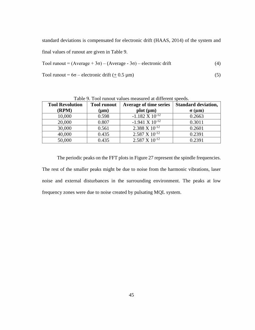
standard deviations is compensated for electronic drift (HAAS, 2014) of the system and

final values of runout are given in Table 9.

Tool runout = (Average + 3σ) – (Average - 3σ) – electronic drift (4)

Tool runout = 6σ – electronic drift (+ 0.5 µm) (5)

Table 9. Tool runout values measured at different speeds.

Tool Revolution

(RPM)

Tool runout

(µm)

Average of time series

plot (µm)

Standard deviation,

σ (µm)

10,000 0.598 -1.182 X 10-12 0.2663

20,000 0.807 -1.941 X 10-12 0.3011

30,000 0.561 2.388 X 10-12 0.2601

40,000 0.435 2.587 X 10-12 0.2391

50,000 0.435 2.587 X 10-12 0.2391

The periodic peaks on the FFT plots in Figure 27 represent the spindle frequencies.

The rest of the smaller peaks might be due to noise from the harmonic vibrations, laser

noise and external disturbances in the surrounding environment. The peaks at low

frequency zones were due to noise created by pulsating MQL system.

46

(a)

Figure 27. Frequency domain plot at different tool rotational speeds (a) 10,000

RPM. (b) 20,000 RPM. (c) 30,000 RPM. (d) 40,000 RPM. (e) 50,000 RPM.

(b)

(µm

)

X: 160 Hz

X: 337 Hz

X: 8 Hz

X: 8 Hz

47

(c)

(d)


X: 514 Hz

X: 691 Hz

(µm

) (µ

m)

X: 8 Hz

X: 8 Hz

48

(e)


A Φ3.175mm plug gage was used for runout measurements. It was observed that

the runout decreases as the tool rotational speed was increased as the machine achieves

stability at high tool rotational speeds (Table 9). Also the measured frequency was a little

different from the theoretical frequency (fz), due to electronic drift in the system.

5.2 TOOL OFFSET

To check the accuracy, consistency and repeatability of tool offset technique

before machining, series of tool offset measurements were conducted and the results are

presented in Figure 28.

X: 868 Hz X: 8 Hz

49

Figure 28. Repeatability and consistency of tool offset values.

From Figure 28, it is clear that the standard deviation of this technique is 0.8 µm.

However, the range of this technique is 2.5 µm which is less than the repeatability of 3

µm as specified by machine manufacturer.

5.3 DETECTION OF BUILT-UP-EDGE

BUE formation is critical factor that directly affects surface finish. There are many

factors responsible for the formation of BUE. A lot depends on machining parameters like

cutting speed, depth of cut, type of lubrication, chip load, workpiece and tool material

combination, tool condition etc. Varying one or combination of the above said factors

would generate different workpiece surfaces. Also BUE formation is intermittent and

highly unpredictable. Formation of BUE is observed with almost all machining parameter

combinations. The intensity or density of BUE’s however are different for different cutting

conditions. To quantify the presence of BUE, it is necessary to successfully identify BUE.

-2

-1.5

-1

-0.5

0

0.5

1

1.5

2

0 5 10 15 20 25 30

Dev

iati

on f

rom

aver

age,

µm

Measurement (#)

Standard deviation = 0.8944 µm

Variance = 0.8 µm

50

BUE can generally be detected at 3 different places after machining:

Rake and clearance surfaces of a cutter after machining

Chips collected during machining

Workpiece surface after machining

The most commonly followed technique to identify BUE is by observing the rake

surface of the tool as seen in Figure 29. During machining the temperatures around chip-

workpiece interaction zone reach favorable temperatures suitable for formation of BUE

(Iwata and Ueda, 1980).

Figure 29. Tool rake surface of uncoated WC after machining 4 slots, length 32 mm,

Uncoated Φ0.406 mm WC flat end mill, 15-80 m/min speed, 15 µm/tooth chip load, 100

µm depth, dry and MQL, A36 carbon steel workpiece.

Another technique is to observe chips for BUE. During machining when chips flow

along the rake surface of milling cutter, BUE on the rake surface might break and weld to

the chip surface as observed in Figure 30. The chips generated after machining are usually

BUE

51

curled. Also since only one side of the chip interacts with the tool rake surface, evidence

for BUE must be searched carefully on only one side. Hence there is a very slim

probability that only a few chips might actually be suitable for viewing.

Figure 30. Scanning electron microscopy image of chips collected after machining pure

titanium, Uncoated WC tool, Φ0.406 mm, 2 flute, 10 m/min speed, 0.2 µm/tooth chip

load, 10 µm depth, dry.

The third place where BUE can be found is the workpiece surface after machining

as seen in Figure 31. The BUE that is welded on to the rake surface shields the actual

cutting edge and acts as a cutting edge. Due to cutting forces involved and growing BUE

size, BUE breaks from the tool and sticks to the surface of workpiece, resulting in poor

surface finish.

BUE

52

In this study, BUE found on machined surface was observed and quantified, while

showing evidence of BUE on tools.

Figure 31. Machined surface of 316L stainless steel with uncoated WC tool, Φ0.406

mm, 2 flute, 10 m/min speed, 0.05 µm/tooth chip load, 30 µm depth, MQL.

5.4 SURFACE ROUGHNESS AND BUILT-UP-EDGE

Zygo surface profiler was used to measure average surface roughness (Sa) and

average line roughness (Ra) of the machined slots on the workpiece to find the correlation

between average surface roughness, linear and area densities of BUE. From Figure 32, 33

and Figure 34, it is quite obvious that as linear and area BUE density increases the

corresponding average line roughness values increase. The correlation between all the

three variables was calculated in Excel to find the degree of linear dependence between

BUE

53

variables (Table 10). Since the values of correlation lie from 0 to 1, we can conclude that

BUE densities, line and surface roughness are positively correlated and BUE density is

one of the reasons for a higher surface roughness.

Table 10. Correlation between Linear density of BUE, Area density of BUE and Line

roughness, Ra, A36 carbon steel, 5 m/min speed, high speed steel tool, Φ3.175 mm, 12

mm length, 3 µm/tooth chip load, 50 µm depth, dry.

Variables Correlation

Linear density versus Line roughness 0.795

Area density versus Line roughness 0.875

Linear density versus Area density 0.938

Figure 32. Linear density of BUE at center of slot, A36 carbon steel, high speed steel

tool, Φ3.175 mm, 12 mm length, 3 µm/tooth chip load, 50 µm depth, dry.

5

10

15

20

1 3 5 7 9 11 13

Lin

ear

Den

sity

of

BU

E (

#/m

m)

Distance from starting location (mm)

5m/min 8m/min 17m/min

54

Figure 33. Area density of BUE at center of slot, A36 carbon steel, high speed steel tool,

Φ3.175 mm, measurement area-15625 µm2, 3 µm/tooth chip load, 50 µm depth, dry.

Figure 34. Average line roughness at center of slot, A36 carbon steel, high speed steel

tool, Φ3.175 mm, 3 µm/tooth chip load, 50 µm depth, dry.

15

20

25

30

1 3 5 7 9 11 13

Are

a d

ensi

ty o

f B

UE

(#

/mm

2)



0.2

0.3

0.4

0.5

0.6

1 3 5 7 9 11 13

Lin

e ro

ughnes

s, R

a(µ

m)



55

5.5 THEORETICAL MODEL

A theoretical model was developed based on following assumptions to predict line

roughness.

Assumptions:

1. Tool edge radius is negligible compared to depth of cut

2. Chip load and depth of cut are much larger than tool edge radius to avoid

ploughing

3. Tool surface and chip has negligible friction

4. Machined surface is free from built-up-edge

The derivation is provided in appendix B. The model is shown in equation (6).

Ra = 0.277 𝑡𝑎𝑛𝛼 𝑓 (6)

Ra = line surface roughness (µm)

f = chip load (µm/tooth)

α = concavity angle of flat end mill (o)

This equation is used to predict line roughness for meso and macro milled surfaces.

Equation 6 proposes that line roughness is directly affected by chip load and concavity

angle which is in strong agreement with previous research on surface finish modeling with

a deviation of 5.4% from equation (2) (Wang and Chang, 2004). Hence to validate this

equation, surface finish data of milled aluminum 6061-T6 are plotted in Figure 35.

56

Figure 35. Predicted and actual line roughness Ra values of slots measured at center. Al

6061-T6, high speed steel tool, Φ3.175 mm, 2 flute, 100 µm depth, dry, 3.5o concavity

angle.

5.6 RESULTS OF MESO MILLING EXPERIMENTS

5.6.1 Surface Roughness

A series of controlled meso milling experiments were conducted on A36 carbon

steel. The experimental conditions are described in Table 6. Surface roughness was used

as a response variable to find the factors that affects the formation of BUE due to their

correlation. A linear regression model was fit using surface roughness as response variable

and cutting speed, depth of cut, tool coating and cutting fluid as input variables (Table 11).

In the second stage of iterations, interaction been input variables were also considered. A

small p-value (less than a significant value, assumed to be 0.1), is required for that

0

0.2

0.4

0.6

0.8

1

1.2

1.4

1.6

1.8

2

2.2

10 20 30 40 50 60 70 80 90 100

Lin

e ro

ughnes

s, R

a, µ

m

Chip load, µm/tooth

60m/min 30m/min

𝑅𝑎 = 0.277 tan(3.5) 𝑓

57

respective input variable to influence surface roughness. A series of iterations were done

and less influential variables were eliminated in successive models. It was found that

cutting speed, depth of cut, cutting fluid and interaction between cutting fluid and depth

of cut effected BUE formation, with cutting speed clearly the dominant factor due its

smallest p-value (Table 11). Also cutting speed and surface roughness are negatively

correlated (negative value of estimate), which means that increasing the cutting speed

decreases the surface finish resulting in smooth surfaces. The next significant factor was

the depth of cut. As the depth of cut increases, amount of rake surface interacting with

chip flow increases, thus providing a larger surface area for workpiece material to stick to

the rake surface of tool increasing the tendency to form BUE. Also using MQL and AlTiN

coated flat end mills improve surface finish due to positive value of estimates.

Equation (7) predicts the surface roughness values based on the estimates for input

variables (Table 11). To predict surface roughness, input variables can be plugged into

equation (7) with a value of ‘1’ for MQL cutting and ‘0’ for dry cutting.

Surface roughness = (0.415) + (0.013*Depth of cut µm) + (0.733*Cutting fluid) -

(0.008*Cutting speed) - (0.013*Depth of cut: Cutting fluid) (7)

The estimate from Table 11 gives the coefficient of each variable in the prediction

equation and with an accuracy level given by standard error. Also the measured values of

surface roughness varied from 0.332 µm-1.539 µm with the low values occurring at high

cutting speeds (80 m/min) and high values occurring at low cutting speeds (15 m/min)

respectively (Figure 36). The raw data are in appendix D.

58

Figure 36. Average surface roughness, Sa, A36 carbon steel, uncoated and coated WC

tool, Φ3.175mm, 4 flutes, 15 µm/tooth chip load.

Table 11. Preliminary linear model fit using R statistical software.

Variable Estimate Std. Error p value

Intercept 0.954000 0.362163 0.0780

Tool coating -0.100000 0.192650 0.6396

Depth of cut 0.015150 0.009632 0.2138

Cutting fluid -0.245000 0.192650 0.2931

Cutting speed -0.007800 0.002964 0.0782

0.200

0.400

0.600

0.800

1.000

1.200

1.400

1.600

0 10 20 30 40 50 60 70 80 90

Surf

ace

roughnes

s, S

a,

µm

Cutting speed, m/min

Uncoated tool, 15m/min speed, 50µm depth, Dry Uncoated tool, 15m/min speed, 100µm depth, MQL

Coated tool, 15m/min speed, 50µm speed, MQL Coated tool, 15m/min speed, 100µm depth, Dry

Uncoated tool, 80m/min speed, 50µm depth, MQL Uncoated tool, 80m/min speed, 100µm depth, Dry

Coated tool, 80m/min speed, 50µm depth, Dry Coated tool, 80m/min speed,100µm depth, MQL

59

Table 12. Final linear model fit using R statistical software


Intercept 0.415000 0.166709 0.08853

Depth of cut -0.012580 0.002004 0.00817

Cutting fluid 0.733000 0.224098 0.04675

Cutting speed -0.007800 0.001090 0.00562

Depth of cut : Cutting fluid -0.013040 0.002835 0.01931

(a) (b)

Figure 37. (a) Uncoated WC tool before machining (b) Tool chipping and wear observed

on uncoated WC tool. Machining 4 consecutive slots, 32 mm length, 15 m/min and 80

m/min speed, 15 µm/tooth chip load, dry and MQL, 50 µm and 100 µm depth, A36

carbon steel.

Tool wear

and chipping

60

(a) (b)

Figure 38. (a) TiAlN coated WC tool before machining (b) Tool chipping and wear

observed on TiAlN coated WC tool. Machining 4 consecutive slots, 32 mm length, 15

m/min and 80 m/min speed, 15 µm/tooth chip load, dry and MQL, 50 µm and 100 µm

depth, A36 carbon steel.

Figure 37(a) and (b) show microscopic images of uncoated WC tool before and

after machining 4 consecutive slots respectively for a total length of 32 mm (Table 6). All

the four cutting edges were observed for evidence of wear and it was found that one of the

cutting edges on both the tools had been chipped. Similar results were observed for AlTiN

coated tool as shown in Figure 38(a) and (b). Also, it was found that wear and chipping

was more for uncoated WC flat end mills over coated WC cutters. The four rake surfaces

were also observed for evidence of BUE after machining 4 slots for a length of 32 mm.

Presence of BUE on the rake surfaces is clearly evident from Figure 39. Workpiece

surfaces were also observed along with the tool rake surfaces.

Tool wear

and chipping

61

Figure 39. Built-up-edge formation observed on rake surfaces of uncoated WC tool.

Machining 4 consecutive slots, 32 mm length, 15 m/min and 80 m/min speed, 15

µm/tooth chip load, dry and MQL, 50 µm and 100 µm depth, A36 carbon steel.


flutes, 15 m/min speed, 15 µm/tooth chip load, 100 µm depth, MQL, Sa=0.997µm.

Figure 40 shows machined surface of A36 steel at the cutting speed of 15 m/min

and chip load of 15 µm/tooth. As seen from the image it is clear that this surface finish is

high when compared to machined surface at 80 m/min cutting speed due to smearing of

BUE

BUE

Direction of

tool rotation

Feed direction

62

BUE on the machine surface (Figure 41). This is evident by visually comparing the chip

load marks on Figure 40 and 41. Lower values of surface roughness (Sa), at high speed is

due to high quality of finished surface without BUE presence. Also, as seen from Figure

36, surface roughness of machined surfaces at 10 m/min were relatively higher compared

to surface roughness of surfaces at 80 m/min irrespective of other machining variables.


flute, 80 m/min speed, 15 µm/tooth chip load, 50 µm depth, MQL, Sa=0.584µm.

5.7 RESULTS OF MICRO MILLING EXPERIMENTS

5.7.1 BUE Density

Area BUE density is used to quantify BUE on the machined surface to qualitatively

compare different machining conditions in micro milling experiments. The detailed

procedure to count and quantify BUE is described in section 4.3.6.3. Formation of BUE

is inevitable and found with all combinations of cutting speeds and chip loads. Figure 42

shows BUE welded on machined surface after breaking off from tool.

Direction of

tool rotation

Feed direction

63

Figure 42. Scanning electron microscopy image of machined 316L stainless steel.

Uncoated WC micro mill, Φ0.406 mm, 10 m/min speed, 0.05 µm/tooth chip load, 30 µm

depth, MQL.

Figure 43. Energy dispersive X-ray spectroscopy (EDS) of BUE.

BUE

Tool rotation direction

Fe

Cr

Fe Ni Mn O

Cr Fe

64

Table 13. Comparison between material composition of 316L stainless steel and BUE

(Azom, 2014) (Steel Grades, 2014).

Material 316L stainless steel

(%weight)

BUE

(%weight)

Cr 16-18 17.7

Ni 10-14 9

O 0 4

Mn <2 1.6

Si <0.75 0.4

Fe Balance 69

Energy dispersive X-ray spectroscopy (EDS) of BUE were done on the SEM

(Figure 43). By comparing the material composition of BUE with that of 316L stainless

steel, we confirm the BUE is from 316L stainless steel (Table 13). Due to the use of MQL

during machining experiments and high temperature in the shear zone, BUE oxidizes

(presence of oxygen in Table 13) and appear as black dots on optical microscopic images.

Figure 44. BUE density showing variation for different grayscale. 27 m/min speed, 1

µm/tooth chip load, uncoated WC tool, Φ0.406 mm WC tool, 30 µm depth, MQL.

3000

3200

3400

3600

3800

4000

4200

4400

4600

4800

5000

1 2 3 4 5 6 7 8 9 10

BU

E d

ensi

ty (

#/m

m2)

Measurements within one slot (#)

Gray scale:75 Gray scale:60

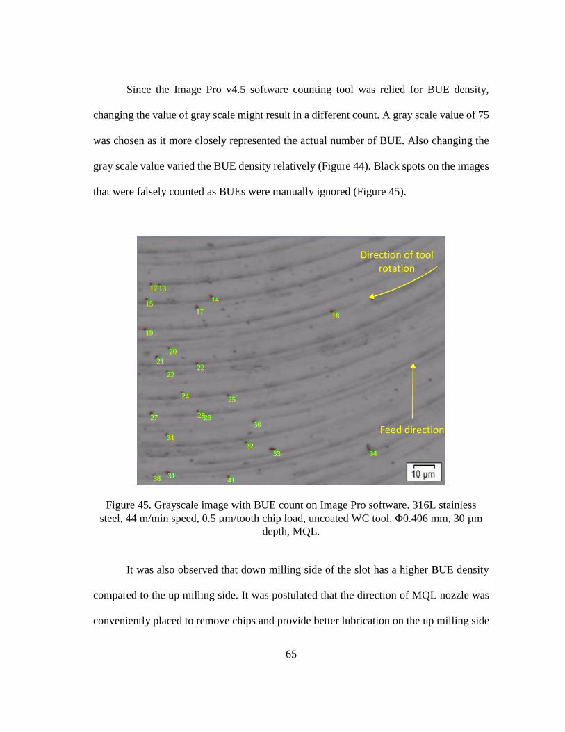
65

Since the Image Pro v4.5 software counting tool was relied for BUE density,

changing the value of gray scale might result in a different count. A gray scale value of 75

was chosen as it more closely represented the actual number of BUE. Also changing the

gray scale value varied the BUE density relatively (Figure 44). Black spots on the images

that were falsely counted as BUEs were manually ignored (Figure 45).


steel, 44 m/min speed, 0.5 µm/tooth chip load, uncoated WC tool, Φ0.406 mm, 30 µm

depth, MQL.

It was also observed that down milling side of the slot has a higher BUE density

compared to the up milling side. It was postulated that the direction of MQL nozzle was

conveniently placed to remove chips and provide better lubrication on the up milling side

Feed direction

Direction of tool rotation

18

12 13

14 15

17

19

20

22 21

22

24 25

27 28 29

31

31 38

30

32 33 34

41

66

over down milling side. This led to increased friction and temperature between chips and

workpiece in the down milling side resulting in higher BUE density (Figures 46-48). Also

during up milling width of chip starts from minimum and increases to a maximum at the

center of slot and might stick to the tool rake surface. As cutting continues to the down

milling side, this further builds up to the tool rake surface resulting in BUE fracture and

subsequent sticking on to the machined surface.

Figure 46. BUE density variation in up and down milling within a sample. 316L

stainless steel, 27 m/min speed, 1 µm/tooth chip load, uncoated WC tool, Φ0.406 mm,

30 µm depth, MQL.

3600

3800

4000

4200

4400

4600

4800

5000

5200

1 2 3 4 5 6 7 8 9 10

BU

E d

ensi

ty (

#/m

m2)

Measurements within a slot (#)

Up milling Down milling

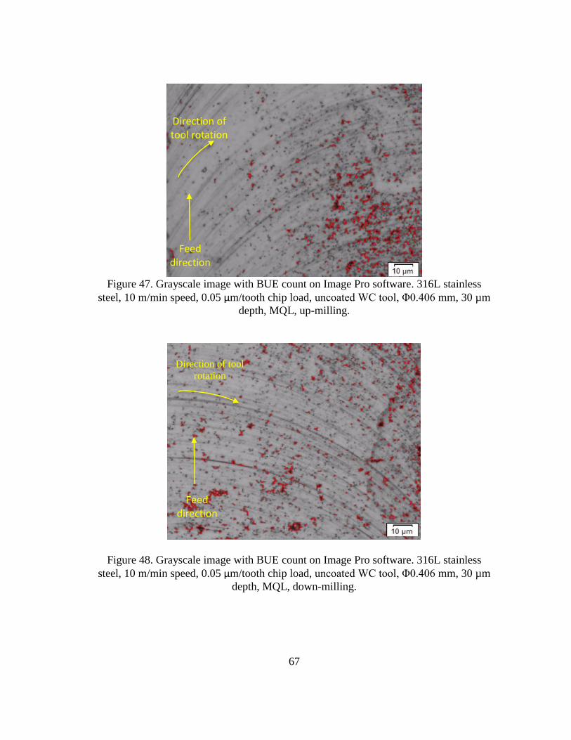
67



depth, MQL, up-milling.



depth, MQL, down-milling.

Feed direction

Direction of tool rotation

Direction of tool

rotation

Feed direction

68

Figure 49. BUE Density (average of 20 samples per slot) on micro milled slots. 316L

stainless steel, 10-60 m/min speed, 0.05-1 µm/tooth chip load, 30 µm depth, Φ0.406 mm

uncoated WC flat end mill, 2 flutes, MQL.

The results of BUE density for each of the machining conditions are presented in

Figure 49. It was observed that BUE density decreases with increasing cutting speeds and

increasing chip loads. Since the minimum cut thickness for most of tool-workpiece

material combinations lie from 20%-30% of their cutting edge radius (re) (0.44-0.66 µm

in this case, since re=2.21 µm) (Yuan et al., 1996), cutting below chip load of 0.5 µm

resulted in ploughing. This led to high BUE density and surface roughness at low chip

loads. Also for the same cutting condition, up milling has lower BUE density over down

0

2000

4000

6000

8000

10000

12000

10 10 10 10 27 27 27 27 44 44 44 44 60 60 60 60

BU

E d

ensi

ty (

#/m

m2)

Cutting Speed, m/min

Up milling (left)Down milling (right)

0.05 µm/tooth, up milling 0.2 µm/tooth, up milling

0.5 µm/tooth, up milling 1 µm/tooth, up milling

0.05 µm/tooth, down milling 0.2 µm/tooth, down milling

0.5 µm/tooth, down milling 1 µm/tooth, down milling

69

milling as discussed before. A combination of low cutting speed and low chip load resulted

in surface with high BUE density and vice versa.

(a) (b)


electron microscopy image of cutting edge of uncoated WC tool, Φ0.406 mm, 10 m/min

speed, 0.05 µm/tooth chip load, 30 µm depth, 24 mm milling length, MQL.

Figure 50 (a) shows the area of flat end mill magnified for viewing tool wear and

BUE. Figure 50 (b) shows SEM image of a cutting edge of uncoated WC tool at cutting

speed of 10 m/min and a chip load of 0.05 µm/tooth for a total milling length of 24 mm.

Tool wear is obvious on the cutting edge. The arrows in Figure 51 (a) point towards the

viewing direction in Figure 51 (b). Also from Figure 51 (b), significant BUE is observed

on the tool cutting edge. Energy dispersive X-ray spectroscopy revealed the presence of

tungsten and cobalt (materials from uncoated WC tool) and iron, cobalt and nickel

(materials from BUE) (Figure 52 and Table 14). Similarly Figure 53 (a) shows area of flat

Tool wear

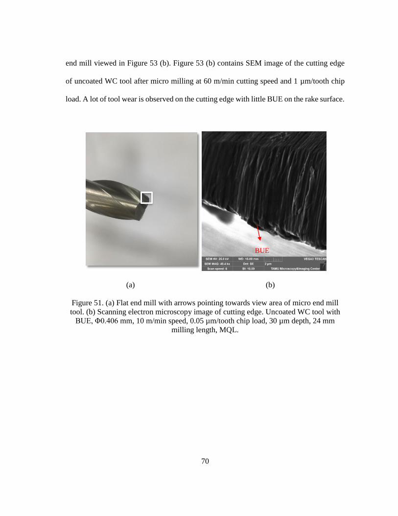
70

end mill viewed in Figure 53 (b). Figure 53 (b) contains SEM image of the cutting edge

of uncoated WC tool after micro milling at 60 m/min cutting speed and 1 µm/tooth chip

load. A lot of tool wear is observed on the cutting edge with little BUE on the rake surface.

(a) (b)

Figure 51. (a) Flat end mill with arrows pointing towards view area of micro end mill

tool. (b) Scanning electron microscopy image of cutting edge. Uncoated WC tool with

BUE, Φ0.406 mm, 10 m/min speed, 0.05 µm/tooth chip load, 30 µm depth, 24 mm

milling length, MQL.

BUE

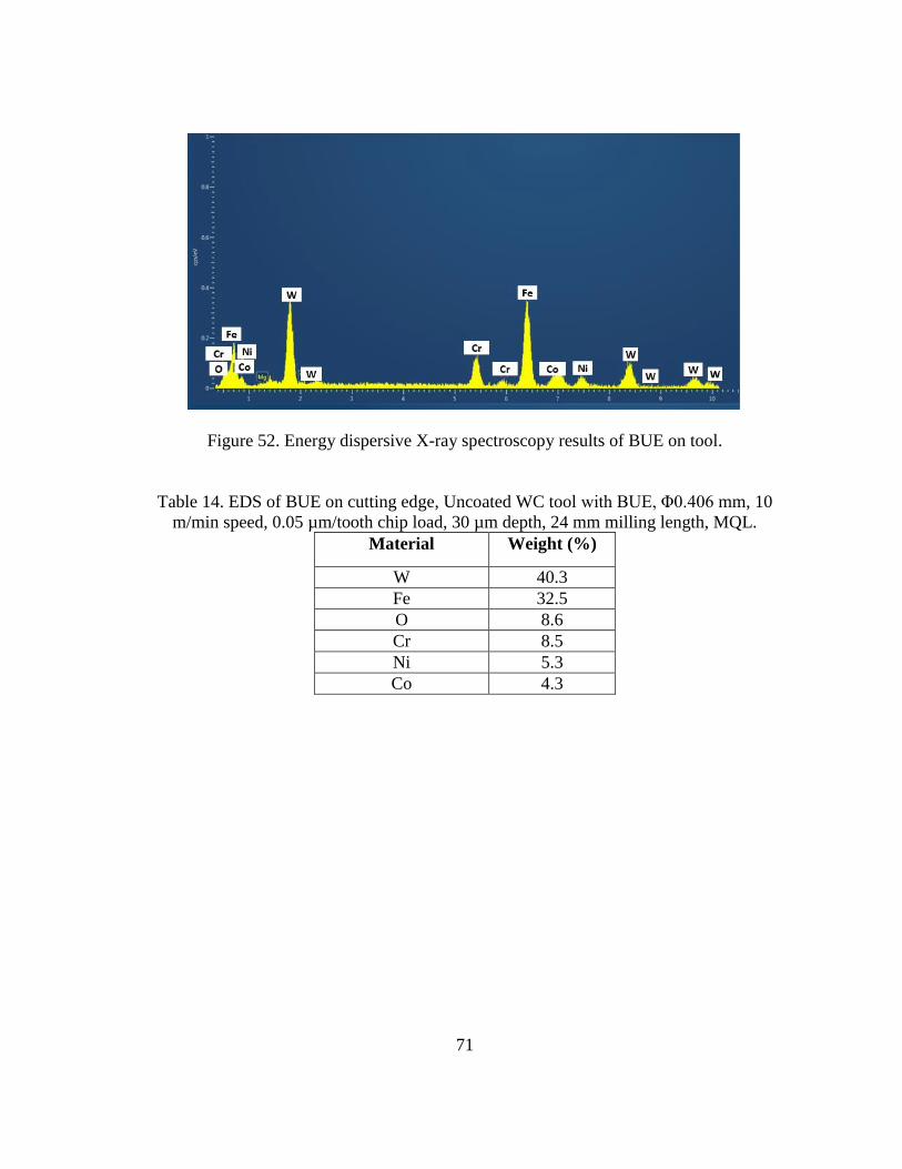
71

Figure 52. Energy dispersive X-ray spectroscopy results of BUE on tool.

Table 14. EDS of BUE on cutting edge, Uncoated WC tool with BUE, Φ0.406 mm, 10

m/min speed, 0.05 µm/tooth chip load, 30 µm depth, 24 mm milling length, MQL.

Material Weight (%)

W 40.3

Fe 32.5

O 8.6

Cr 8.5

Ni 5.3

Co 4.3

72

(a) (b)


electron microscopy image of rake surface and cutting edge. Uncoated WC tool with

BUE, Φ0.406 mm, 60 m/min speed, 1 µm/tooth chip load, 30 µm depth, 24 mm milling

length, MQL.

Figure 54 (a) shows the area of a flute magnified for viewing BUE. Figure 54 (b)

shows BUE formed after machining pure titanium with Φ0.8 mm AlTiN coated WC tool

for 4 slots of 12 mm each at chip loads of 2,4,6 and 8 µm/tooth and 10 m/min cutting

speed. Since the same cutting tool was used for milling all the 4 slots, considerable tool

wear and BUE was observed on the cutting edge and rake surface.

BUE

Tool wear

73

(a) (b)


electron microscopy image of rake surface and cutting edge. AlTiN WC tool with BUE,

Φ0.800 mm, 10 m/min speed, 2-8 µm/tooth chip load, 30 µm depth, 48 mm milling

length, MQL.

5.7.2 Surface roughness

Average roughness values (Sa) were between 0.1 µm to 0.2 µm for cutting speeds

below 30 m/min and there was shift in roughness values to below 0.1 µm when milling at

cutting speeds increased over 40 m/min (Figure 55). Childs (2011) reported that as cutting

speed increases from 0.5 m/min to 40 m/min, the maximum temperature at rake surface

increases from 80 oC to 500 oC and at low temperatures the strain rate levels led to BUE

formation. This can be avoided by machining at cutting speeds >40 m/min. The raw data

for surface roughness are tabulated in appendix D.

BUE

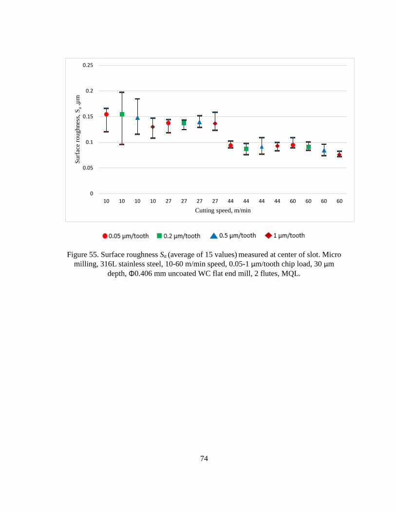
74

Figure 55. Surface roughness Sa (average of 15 values) measured at center of slot. Micro

milling, 316L stainless steel, 10-60 m/min speed, 0.05-1 µm/tooth chip load, 30 µm

depth, Φ0.406 mm uncoated WC flat end mill, 2 flutes, MQL.

0

0.05

0.1

0.15

0.2

0.25

10 10 10 10 27 27 27 27 44 44 44 44 60 60 60 60

Surf

ace

roughnes

s, S

a,µ

m


75


316L stainless steel, Φ0.406 mm uncoated WC tool, 2 flute, 10-60 m/min speed, 0.05-1

µm/tooth chip load, 30 µm depth, MQL, 7o concavity angle.

Equation (6) was used to predict line roughness of micro milled slots on 316L

stainless steel workpiece. According to equation (6), chip load and concavity angle of tool

determined the line roughness, under the assumption that surface was free from BUE. It

can be observed from Figure 56 that when the line roughness was measured at places in

absence of BUE, the equation performed considerably well in predicting the line

roughness accurately. However, when the line roughness was measured at places in

presence of BUE, the equation failed to predict accurately. This is because BUE masks

the actual effect of chip load on line roughness. Figure 57 shows surface finish data of

micro milling of 316L stainless steel and meso milling of aluminum 6061-T6 combined

into single plot.

0.00

0.02

0.04

0.06

0.08

0.10

0.12

0.14

0.16

0.18

0.20

0 0.2 0.4 0.6 0.8 1 1.2

Lin

e ro

ughnes

s, R

a, µ

m


60m/min (without BUE) 10m/min (without BUE)

10m/min (with BUE) 60m/min (with BUE)

𝑅𝑎 = 0.277 tan(7) 𝑓

76


316L stainless steel: Φ0.406 mm uncoated WC tool, 2 flute, 10-60 m/min speed,

0.05-1 µm/tooth chip load, 30 µm depth, MQL, 7o concavity angle.

Pure titanium: Φ0.8 mm AlTiN coated WC tool, 1 flute, 10 m/min speed, 2-8

µm/tooth chip load, 30 µm depth, dry, 5.2o concavity angle.

6061-T6 aluminum: Φ3.175 mm uncoated high speed steel tool, 2 flute, 60

m/min speed, 12.7-101.6 µm/tooth chip load, 100 µm depth, dry, 3.5o concavity

angle.

5.7.3 Tool wear

Tool wear was also observed during micro milling 316L stainless steel with

uncoated WC flat end mills. Average tool wear was calculated as area loss of cutting tool

material at the cutting edge radius on both the flutes of a milling cutter (Figure 58-59).

The area loss was multiplied by the depth of cut to get the volumetric loss.

0.05

0.50

0.01 0.1 1 10 100

Lin

e ro

ughnes

s, R

a, µ

m


60m/min (without BUE) 10m/min (without BUE)

10m/min (with BUE) 60m/min (with BUE)

60m/min (Meso milling) 10m/min (AlTiN coated, without BUE)

Ra = 0.277 tan (5.2) f

Micro milling Meso milling

Ra = 0.277 tan (3.5) f

Ra = 0.277 tan (7) f

77

(a) (b)

Figure 58. (a) Top view of new micro tool (b) Top view of micro tool after 24 mm

milling distance, 316L stainless steel, 27 m/min speed, 1 µm/tooth chip load, Φ0.406

mm uncoated WC tool, 30 µm depth, MQL.

(a) (b)

Figure 59 (a) Top view of machined tool superimposed on top view of new micro tool

(b) One of the cutting edges magnified to calculate tool wear and chipping after milling

24 mm, 316L stainless steel, 27 m/min speed, 1 µm/tooth chip load, Φ0.406 mm

uncoated WC tool, 30 µm depth, MQL.

Tool wear and

chipping

78

Since the cutting conditions (chip load and cutting speed) are different for each

slot, machining times are different for each slot as shown in Table 15. All the slots were

machined for an equal distance of 24 mm with unequal milling times. The wear rate (after

each second of machining time) and tool wear per machining length were calculated for

comparison.

Table 15. Tool wear and chipping for micro milling experimental conditions, 316L

stainless steel workpiece, Φ0.406 mm uncoated WC tool, MQL

Cu

ttin

g

spee

d

(m/m

in)

Ch

ip L

oad

,

(µm

/to

oth

)

Tota

l

mach

inin

g

tim

e

(seco

nd

s)

Aver

age

tool

wea

r

(µm

3)

Tool

wea

r

rate

(µm

3/s

ec)

Tool

wea

r

per

mach

inin

g

len

gth

(µm

3/m

m)

10

0.05 918.5 3535 2 147

0.2 340.2 4348 6 181

0.5 208.7 2683 6 111

1 153.1 1491 5 62

27

0.05 229.6 4341 9 181

0.2 85.0 3681 22 153

0.5 52.2 2511 24 105

1 38.3 2931 38 122

44

0.05 91.8 12255 67 511

0.2 34.0 7632 112 318

0.5 20.9 1941 46 81

1 15.3 1797 59 75

60

0.05 45.9 6293 69 262

0.2 17.0 4261 125 178

0.5 10.4 1474 71 61

1 7.7 2587 169 108

79

Figure 60. Average tool volumetric loss per machining length after micro machining

slots with 10-60 m/min cutting speed, 0.05-1 µm/tooth chip load, 30 µm depth, Φ0.406

mm uncoated WC flat end mill, 2 flutes, 316L stainless steel workpiece.

Figure 60 shows that tool wear per machining length is highly dependent on chip

load and speed. As chip load was increased from 0.05 µm/tooth to 1 µm/tooth, tool wear

decreased for the same milling distance. For the same distance, the distance travelled by

tool edge radius is more at low chip loads over high chip loads resulting in large tool wear

at low chip loads. Also for same chip loads, tool wear increases with increase in cutting

speed. The results agreed well with study conducted by Rahman et al. (2001) on micro

milling copper where they suggested that tool wear increases with decrease in depth of cut

and increase in cutting speed. Although tool wear increases at high cutting speeds, a

0

100

200

300

400

500

600

10 10 10 10 27 27 27 27 44 44 44 44 60 60 60 60

To

ol

wea

r p

er m

achin

ing l

ength

(µ

m3/m

m)


0.05 µm/tooth 0.2 µm/tooth 0.5 µm/tooth 1 µm/tooth

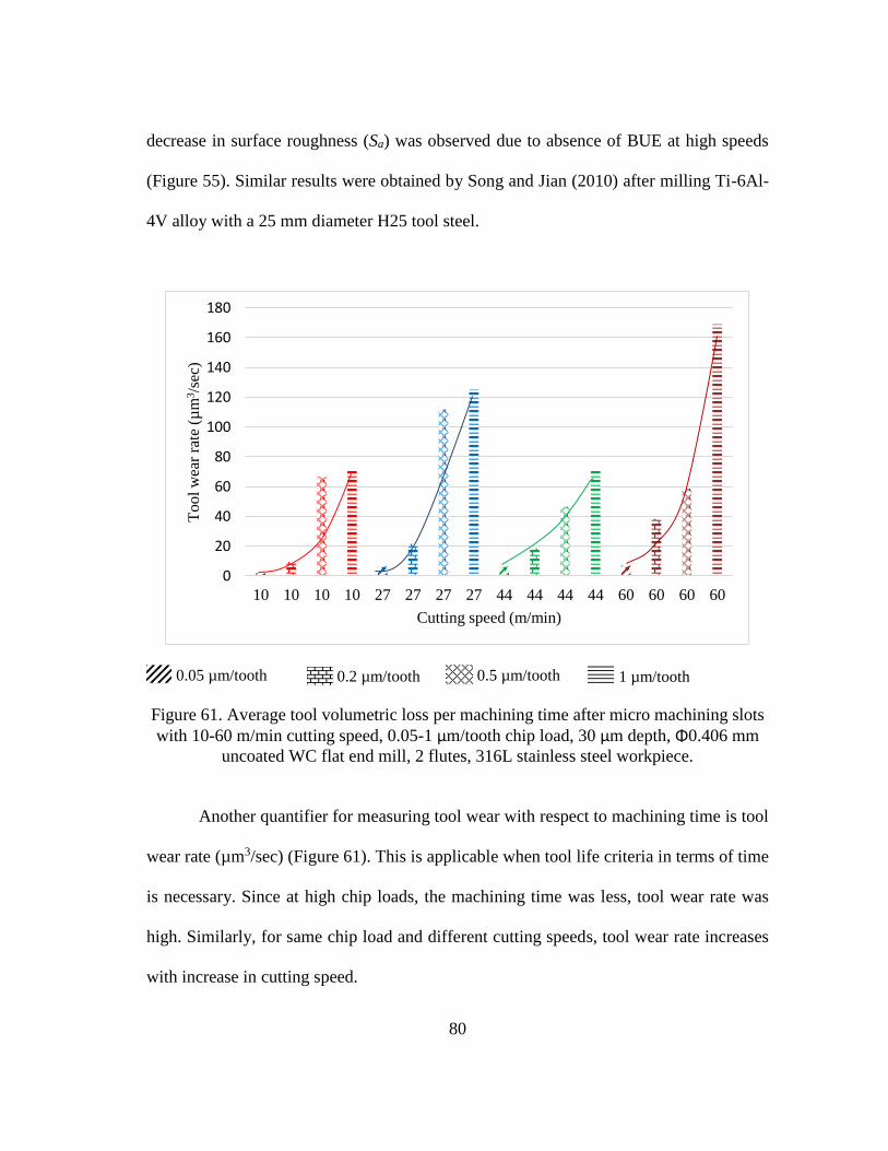
80

decrease in surface roughness (Sa) was observed due to absence of BUE at high speeds

(Figure 55). Similar results were obtained by Song and Jian (2010) after milling Ti-6Al-

4V alloy with a 25 mm diameter H25 tool steel.

Figure 61. Average tool volumetric loss per machining time after micro machining slots

with 10-60 m/min cutting speed, 0.05-1 µm/tooth chip load, 30 µm depth, Φ0.406 mm

uncoated WC flat end mill, 2 flutes, 316L stainless steel workpiece.

Another quantifier for measuring tool wear with respect to machining time is tool

wear rate (µm3/sec) (Figure 61). This is applicable when tool life criteria in terms of time

is necessary. Since at high chip loads, the machining time was less, tool wear rate was

high. Similarly, for same chip load and different cutting speeds, tool wear rate increases

with increase in cutting speed.

0

20

40

60

80

100

120

140

160

180

10 10 10 10 27 27 27 27 44 44 44 44 60 60 60 60

Tool

wea

r ra

te(µ

m3/s

ec)

Cutting speed (m/min)

0.05 µm/tooth 0.2 µm/tooth 0.5 µm/tooth 1 µm/tooth

81

5.7.4 Surface roughness prediction including BUE density and tool wear volume

Formation of BUE in micro milling was prevalent and therefore equation (6) is not

able to accurately predict line roughness. Hence a new model including the effect of BUE

is developed. A null hypothesis is assumed that this difference (delta) between actual

roughness and predicted roughness due to equation (6) is not due to BUE and tool wear.

Ra = 0.277 tan (α) f + Δ (8)

A model is fit in R with BUE and tool wear as variables and this difference as

response variable. It is observed from Table 16 that both BUE and tool wear are significant

predictors of delta due to their small p-values and thus the null hypothesis is rejected.


roughness and actual roughness


Intercept -2.263 x 10-01 5.375 x 10-02 0.00102

BUE density (#/mm2) 3.575 x 10-05 9.790 x 10-06 0.00293

Tool wear volume (µm3) 1.890 x 10-05 6.042 x 10-06 0.00799

Δ = (3.575 x 10-05 * BUE) + (1.890 x 10-05 * tool wear volume) (9)

Ra = 0.277 tan (α) f + (3.575 x 10-05 * BUE) + (1.890 x 10-05 * tool

wear volume) (10)

Hence a model including the effect of BUE and tool wear is added to equation (6).

Equation (10) is able to predict line roughness accurately for micro milling considering

the effect of BUE and tool wear.

82

Also, a model is developed to study the effect of input variables on BUE formation

(Equation 11). Cutting speed, chip load, tool wear and interaction among them are fit with

BUE density as response variable. After series of iterations, unimportant variables are

removed from successive models and it is found that cutting speed has significant

influence on BUE (Table 17).


roughness and actual roughness


Intercept 7708.40 971.29 2.44 x 10-06

Chip load (µm/tooth) 4264.33 3243.31 0.2113

Cutting speed (m/min) -144.33 63.04 0.0394

BUE density = 7708.40 + (4264.33 chip load) - (144.33 * cutting speed) (11)

5.7.5 Surface roughness prediction including BUE density and tool wear volume using

curve fitting

A new model including the effect of BUE is developed by combining equation (6)

with data fitting line as in equation (12).

Ra (micro range) = 0.0061 f + 0.0872 (12)

The above model is a linear fit of the difference between actual line roughness and

predicted line roughness (equation (6)). This difference, delta is considered to be due to

BUE formation in micro milling. Thus a modified equation, combining equation (6) and

(12) can be used to predict line roughness for both meso and micro milling (equation (13)).

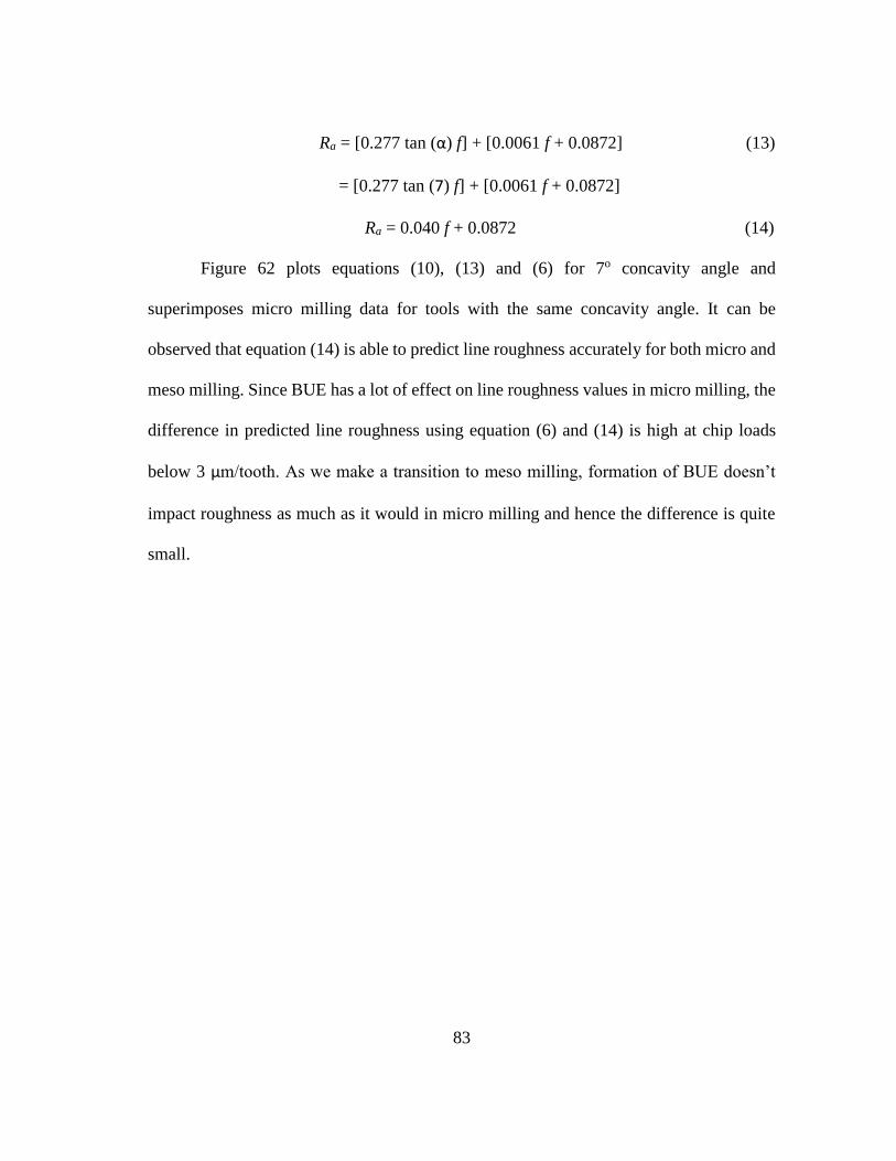
83

Ra = [0.277 tan (α) f] + [0.0061 f + 0.0872] (13)

= [0.277 tan (7) f] + [0.0061 f + 0.0872]

Ra = 0.040 f + 0.0872 (14)

Figure 62 plots equations (10), (13) and (6) for 7o concavity angle and

superimposes micro milling data for tools with the same concavity angle. It can be

observed that equation (14) is able to predict line roughness accurately for both micro and

meso milling. Since BUE has a lot of effect on line roughness values in micro milling, the

difference in predicted line roughness using equation (6) and (14) is high at chip loads

below 3 µm/tooth. As we make a transition to meso milling, formation of BUE doesn’t

impact roughness as much as it would in micro milling and hence the difference is quite

small.

84


316L stainless steel, Φ0.406 mm uncoated WC tool, 2 flute, 10-60 m/min speed, 0.05-1

µm/tooth chip load, 30 µm depth, MQL, 7o concavity angle.

0.00

0.01

0.10

1.00

10.00

0.01 0.1 1 10 100 1000

Lin

e ro

ughnes

s, R

a, µ

m


60m/min (without BUE, 316L SS) 10m/min (without BUE, 316L SS)

60m/min (with BUE, 316L SS) 10m/min (with BUE, 316L SS)

Ra = 0.277 tan (7) f + 0.0061 f + 0.0872

Ra = 0.277 tan (7) f + (3.575 x 10-05 * BUED) +

(1.890 x 10-05 * TWV)

Ra = 0.277 tan (7) f

85

6. CONCLUSIONS

Meso milling of Aluminum 6061 T6, A36 carbon steel and micro milling of 316L

stainless steel were carried out. The experimental study shows:

1. A surface finish model was derived for both meso and micro milling; the line

roughness Ra is a function of chip load and tool concavity angle. At chip loads

below 3 µm/tooth, where the effect of BUE on line roughness is significant, the

surface finish model predicted a higher line roughness over conditions in absence

of BUE. However as we increase the chip loads above 3 µm/tooth, the effect of

BUE on roughness is small and the difference between predicted roughness in

presence of BUE and absence of BUE is small.

2. A combination of high cutting speed with MQL resulted in best surface finish in

meso milling of A36 carbon steel. It was also observed that AlTiN coated WC

tools produce less BUE and smooth surface finish compared to uncoated WC tools.

3. Built-up-edge density is high at low cutting speeds (<30 m/min) and low at high

cutting speeds (>40 m/min). Also BUE formation is minimal at high chip load

conditions. This is because of shear dominated cutting mechanism at high chip

loads and ploughing dominated cutting mechanism at low chip loads.

4. Surface roughness is low at high cutting speeds (>40 m/min) and high at low

cutting speeds (<30 m/min). However tool wear per machining length is more at

high cutting speeds. Hence, to achieve a smooth surface with minimum BUE and

longer tool life, higher cutting speeds (>40 m/min) and chip loads (> 0.5 µm/tooth)

are to be selected.

86

7. RECOMMENDATIONS AND FUTURE WORK

1. This research can be extended to different type of tool coatings and other

workpiece materials to study effect of BUE on surface roughness on wide range of

chip loads. Also this data can be used to test the validity of combined line

roughness model proposed which compensates for BUE formation in milling. A

BUE adhesion and welding to cutting tool depends on the surface of tool material

and cutting condition.

2. Study of BUE density and machining conditions by observing machined chips.

3. Analyze tool vibration data to detect BUE.

4. Tool diameters with 0.050 mm can be machined with CNC milling machines

capable of reaching 200,000 RPM and 400,000 RPM for cutting speeds of 30

m/min and 60 m/min respectively.

5. A device for tool offset measurements can be developed to shorten set up time for

micro milling experiments.

6. Using atomic force microscope (AFM) to measure surface roughness of micro

milled surface while avoiding BUE.

87

REFERENCES

Aramcharoen, A., Mativenga, P.T., 2009. Size effect and tool geometry in micromilling

of tool steel. Precision Engineering 33, 402-407.

Aramcharoen, A., Mativenga, P.T., Yang, S., Cooke, K.E., Teer, D.G., 2008. Evaluation

and selection of hard coatings for micro milling of hardened tool steel. International

Journal of Machine Tools and Manufacture 48, 1578-1584.

AZoM™. Grade 316L, A36 – properties, fabrication and applications, [Online].

Available: http://www.azom.com/ [Accessed Dec 22, 2014].

Bourne, M.A., 2007. A Consumer's Guide to MEMS & Nanotechnology. Bourne

Research [Accessed Nov 19, 2014].

Byrne, G., Dornfeld, D., Denkena, B., 2003. Advancing Cutting Technology. CIRP

Annals - Manufacturing Technology 52, 483-507.

Childs, T.H.C., 2011. Towards simulating built-up-edge formation in the machining of

steel. CIRP Journal of Manufacturing Science and Technology 4, 57-70.

Clausing Industrial, Surface grinder properities, [Online]. Available: http://www.clausing-

industrail.com/ [Accessed Jan 29, 2015].

Cui, X., Zhao, J., Jia, C., Zhou, Y., 2012. Surface roughness and chip formation in high-

speed face milling AISI H13 steel. The International Journal of Advanced

Manufacturing Technology 61, 1-13.

Dmytro, B., 2013. Surface finish modeling in micro milling of biocompatible materials.

Texas A&M University, College Station.

Fang, N., Pai, P.S., Edwards, N., 2010. Prediction of built-up edge formation in

machining with round edge and sharp tools using a neural network approach.

International Journal of Computer Integrated Manufacturing 23, 1002-1014.

Furukawa, Y., Moronuki, N., 1988. Effect of Material Properties on Ultra Precise

Cutting Processes. CIRP Annals - Manufacturing Technology 37, 113-116.

Groover, M.P. (2004). Fundamentals of Modern Manufacturing. New York: John Wiley

& Sons.

HAAS CNC, OM2 milling machine, [Online]. Available: http://www.haascnc.com/

[Accessed Oct 18, 2014].

88

Heginbotham, W., Gogia, S., 1961. Metal cutting and the built-up nose. Proceedings of

the Institution of Mechanical Engineers 175, 892-917.

Ikawa, N., Shimada, S., Tanaka, H., 1992. Minimum thickness of cut in

micromachining. Nanotechnology 3(1), 6.

Iwata, K., Ueda, K., 1980. Fundamental analysis of the mechanism of built-up edge

formation based on direct scanning electron microscope observation. Wear 60, 329-337

52.

Keyence sensors, Keyence LK-G82 laser displacement sensor, [Online]. Available:

http://www.keyence.com/ [Accessed March 14, 2015].

Lai, X., Li, H., Li, C., Lin, Z., Ni, J., 2008. Modelling and analysis of micro scale

milling considering size effect, micro cutter edge radius and minimum chip thickness.

International Journal of Machine Tools and Manufacture 48, 1-14.

Liu, X., DeVor, R.E., Kapoor, S., Ehmann, K., 2004. The mechanics of machining at the

microscale: assessment of the current state of the science. Journal of manufacturing

science and engineering 126, 666-678.

Masaki, T., Kawata, K., Masuzawa, T., 1990. Micro electro-discharge machining and its

applications, Micro Electro Mechanical Systems, 1990. Proceedings, An Investigation of

Micro Structures, Sensors, Actuators, Machines and Robots. IEEE. IEEE, pp. 21-26.

Masuzawa, T., 2000. State of the Art of Micromachining. CIRP Annals - Manufacturing

Technology 49, 473-488.

McKeown, P., 1986. High precision manufacturing and the British economy.

Proceedings of the Institution of Mechanical Engineers, Part B: Journal of Engineering

Manufacture 200, 147-165.

MSC Industrial Supply, Meso tool properties, [Online]. Available:

http://www.mscdirect.com/ [Accessed Nov 24, 2014].

Oberg, E., Jones, F., Horton H., Ryfeel H., 2009. Machinery’s hand book 29th edition,

New York: Industrial Press Inc,.

Olympus corporation, Optical microscope, [Online]. Available:

http://www.olympusamerican.com/ [Accessed Oct 29, 2014].

Peng, F.Y., Wu, J., Yuan, S., Yan, R., 2012. The Effect of Vibration on the Surface

Topography in Micro-Milling. Applied Mechanics and Materials 217, 1791-1801.

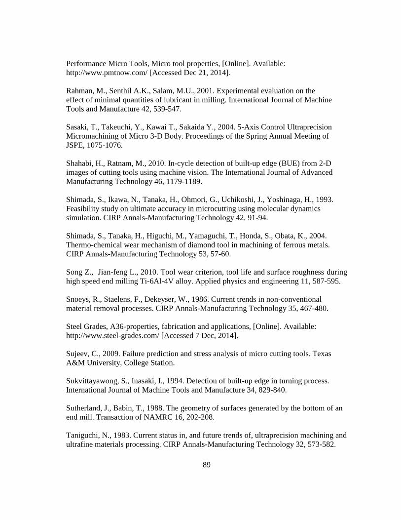
89

Performance Micro Tools, Micro tool properties, [Online]. Available:

http://www.pmtnow.com/ [Accessed Dec 21, 2014].

Rahman, M., Senthil A.K., Salam, M.U., 2001. Experimental evaluation on the

effect of minimal quantities of lubricant in milling. International Journal of Machine

Tools and Manufacture 42, 539-547.

Sasaki, T., Takeuchi, Y., Kawai T., Sakaida Y., 2004. 5-Axis Control Ultraprecision

Micromachining of Micro 3-D Body. Proceedings of the Spring Annual Meeting of

JSPE, 1075-1076.

Shahabi, H., Ratnam, M., 2010. In-cycle detection of built-up edge (BUE) from 2-D

images of cutting tools using machine vision. The International Journal of Advanced

Manufacturing Technology 46, 1179-1189.

Shimada, S., Ikawa, N., Tanaka, H., Ohmori, G., Uchikoshi, J., Yoshinaga, H., 1993.

Feasibility study on ultimate accuracy in microcutting using molecular dynamics

simulation. CIRP Annals-Manufacturing Technology 42, 91-94.

Shimada, S., Tanaka, H., Higuchi, M., Yamaguchi, T., Honda, S., Obata, K., 2004.

Thermo-chemical wear mechanism of diamond tool in machining of ferrous metals.

CIRP Annals-Manufacturing Technology 53, 57-60.

Song Z., Jian-feng L., 2010. Tool wear criterion, tool life and surface roughness during

high speed end milling Ti-6Al-4V alloy. Applied physics and engineering 11, 587-595.

Snoeys, R., Staelens, F., Dekeyser, W., 1986. Current trends in non-conventional

material removal processes. CIRP Annals-Manufacturing Technology 35, 467-480.

Steel Grades, A36-properties, fabrication and applications, [Online]. Available:

http://www.steel-grades.com/ [Accessed 7 Dec, 2014].

Sujeev, C., 2009. Failure prediction and stress analysis of micro cutting tools. Texas

A&M University, College Station.

Sukvittayawong, S., Inasaki, I., 1994. Detection of built-up edge in turning process.

International Journal of Machine Tools and Manufacture 34, 829-840.

Sutherland, J., Babin, T., 1988. The geometry of surfaces generated by the bottom of an

end mill. Transaction of NAMRC 16, 202-208.

Taniguchi, N., 1983. Current status in, and future trends of, ultraprecision machining and

ultrafine materials processing. CIRP Annals-Manufacturing Technology 32, 573-582.

90

Tescan Vega 3, Scanning electron microscope, [Online]. Available:

http://www.tescan.com/ [Accessed April 15, 2015].

UNIST fluid systems, Oil Mist lubrication, [Online]. Available: http://www.unist.com/

[Accessed Dec 11, 2014].

Vogler, M.P., DeVor, R.E., Kapoor, S.G., 2004. On the modeling and analysis of

machining performance in micro-endmilling, Part I: Surface generation. Journal of

Manufacturing Science and Engineering 126, 685-694.

Wang, M.-Y., Chang, H.-Y., 2004. Experimental study of surface roughness in slot end

milling AL2014-T6. International Journal of Machine Tools and Manufacture 44, 51-57.

Weule, H., Hüntrup, V., Tritschler, H., 2001. Micro-cutting of steel to meet new

requirements in miniaturization. CIRP Annals-Manufacturing Technology 50, 61-64.

Yuan, Z., Zhou, M., Dong, S., 1996. Effect of diamond tool sharpness on minimum

cutting thickness and cutting surface integrity in ultraprecision machining. Journal of

Materials Processing Technology 62, 327-330.

Zawawi, M.Z., Shaharudin, M.A.H., Manaf, A.R.A., 2014. Influences of Varying

Combination of Feed Rate and Depth of Cut to Tool Wear Rate and Surface Roughness:

High Speed Machining Technique in Non-High Speed Milling Machine. Advanced

Materials Research 903, 194-199.

Zorev, N.N., 1966. Metal cutting mechanics. Pergamon, Headington hill hall, Oxford,

England. 1966, 526P.

Zygo 3D optical surface profiler, Surface roughness measurements, [Online]. Available:

http://www.zygo.com/ [Accessed Nov 28, 2014].

91

APPENDIX A

SPECIFICATIONS OF EQUIPMENT

A.1 HAAS OM2 CNC Milling machine

The HAAS OM2 milling machine is a 5 axis machine (X, Y, Z, A and B).

Specifications:

1. The maximum travel for X, Y and Z axis are 305 mm x 254 mm x 305 mm

respectively.

2. The spindle runs on air bearings with a minimum rotational speed of 1000 RPM

and maximum speed of 50,000 RPM.

3. The maximum rapid feed rate is 19.2 m/min and maximum cutting feed rate is 12.7

m/min.

4. The positioning accuracy is +5 µm and repeatability is +3 µm.

Figure A.1 HAAS OM2 CNC milling machine (HAAS, 2014)

92

A.2 CLAUSING CSG818H Surface Grinder

Specifications:

1. The table size for the surface grinder is 203 mmX460 mm with a maximum

grinding length of 480 mm and maximum grinding width of 238 mm.

2. The grinding spindle drive is powered by a 2 HP motor with a speed of 3450 RPM.

3. The diameter of the standard grinding wheel is 203 mm and width between 12.7

mm-19 mm.

Figure A.2 CLAUSING Surface grinder (Clausing, 2014)

A.3 UNIST lubrication system

1. Unist lubrication system was used to supply micro-mist during machining.

2. A liquid metering pump exists to generate 5-200 pulse/minute.

3. An air metering screw exists to control the flow of air atomizing out the nozzle.

93

4. The amount of coolant (drops per cycle) and ratio of coolant to pressurized air can

be adjusted according to needs.

5. Cool lube 2210 was used as a lubricant for cooling workpiece and tool. It reduces

coefficient of friction, µ at tool and workpiece interface.

Figure A.3 UNIST micro mist system with its components (Unist, 2015)

A.4 Olympus optical microscope

1. Olympus STM6 with a motorized 3-axis type microscope was used.

2. The dimensions of the observation table are 465 mmX437 mm. The minimum

readout on the counter was 0.1 µm

3. Repeatability of objective lens with 10X and 20X was 2 µm and with 50X was 1

µm

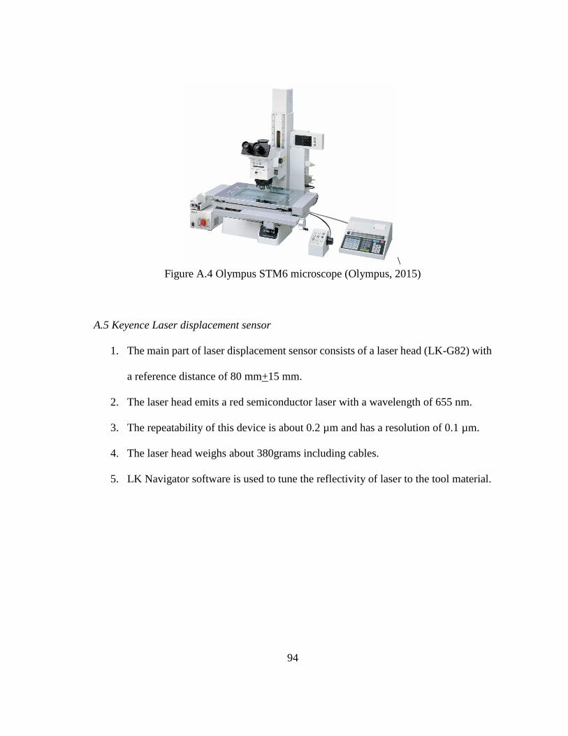
94

\

Figure A.4 Olympus STM6 microscope (Olympus, 2015)

A.5 Keyence Laser displacement sensor

1. The main part of laser displacement sensor consists of a laser head (LK-G82) with

a reference distance of 80 mm+15 mm.

2. The laser head emits a red semiconductor laser with a wavelength of 655 nm.

3. The repeatability of this device is about 0.2 µm and has a resolution of 0.1 µm.

4. The laser head weighs about 380grams including cables.

5. LK Navigator software is used to tune the reflectivity of laser to the tool material.

95

Figure A.5 CAD drawing of Keyence LKG-08 laser head (Keyence, 2015)

A.6 Zygo ZeGage 3D optical surface profiler

1. The physical dimensions of the workstation table are 74 cm X 127 cm X 76 cm

and weighs 37 kilograms.

2. The part stage is an integrated T-slot plate with a travel of 50 mm X 100 mm

travel in both X and Y directions. It tips/tilts to an angle of 40.

3. The Z-stage has a travel of 100 mm and has a 10X objective lens attached.

4. The Zygo ZeGage comes with a ZeMaps software integrated with inbuilt

functions for image processing.

96

5. The surface topography has a repeatability of less than 3.5 nm with a data scan

rate of less than 23 µm/sec.

Figure A.6 Zygo ZeGage 3D optical surface profiler (Zygo, 2015)

A.7 TESCAN Vega LM3

1. The Vega LM3 has a tungsten heated cathode electron gun. The resolution is 3 nm at

30kV/2 nm at 30kV. The chamber pressure is less than 9 X 10-3 Pa.

2. The magnification can be varied from 2x-100000x.

3. The scanning speed varies from 20 ns to 10 ms per pixel adjustable in steps.

4. The table movement is Comp centric, fully motorized with a movement of 80 mm, 60

mm and 47 mm in X, Y and Z direction respectively. Also the table can be rotated 3600

and can be tilted from -800 to 800.

97

Figure A.7 TESCAN Vega LM3 scanning electron microscope (TESCAN, 2015).

98

APPENDIX B

MODELLING OF LINE SURFACE ROUGHNESS IN FLAT END MILLING

Figure B.1 Geometrical sketch representing simulated surface of a flat end mill

Figure B.1 is assumed to be the surface simulated by a flat end mill cutter. The concavity

angle of the tool is a geometric property of the tool and depends on the manufacturer. It is

assumed that the concavity angle effects the final geometry of the machined surface.

∠EOC=α be the concavity angle

EC = t = Rmax be the maximum height of surface profile

OE = f = chip load

1. The center of gravity for a right angle triangle is at a distance of 1/3 from X-axis

and 1/3 from the perpendicular side inside the triangle. Hence the dashed line is at

a height t/3 from X-axis.

𝐷𝐸 = 1

3𝐸𝐶

𝐷𝐸 =1

3𝑡 (B1)

2. Also, Triangles CBD and COE are similar to each other

X

Y

99

𝐶𝐷

𝐶𝐸=

𝐵𝐷

𝑂𝐸

2

3=

𝐵𝐷

𝑂𝐸

𝐵𝐷 =2

3 𝑂𝐸 (B2)

3. The value of AB can be found by subtracting BD from OE

𝐴𝐵 = 𝑂𝐸 − 𝐵𝐷

𝐴𝐵 = 𝑂𝐸 −2

3𝑂𝐸

𝐴𝐵 =1

3𝑂𝐸

𝐴𝐵 =1

3 𝑓 (B3)

4. Tangent of Concavity angle is calculated

𝑡𝑎𝑛𝛼 =𝑡

𝑓(B4)

𝑡 = 𝑓 ∗ 𝑡𝑎𝑛𝛼 (B5)

100

Figure B.2 Line roughness is calculated as the arithmetic average of infinitesimally small

areas along a given length.

Let h1, h2, h3…hn etc. be infinitesimally height of a surface when moving the same

distance along the machined surface. The arithmetic average Ra is defined as

Ra = (ℎ1+ℎ2+ℎ3….ℎ𝑛)

𝑛 (B6)

𝑅𝑎 =(ℎ1Δx + ℎ2Δx+ℎ3Δx … . ℎ𝑛Δx)

𝑛 ∗ Δ𝑥

𝑅𝑎 =(𝐴1+𝐴2+𝐴3 … . 𝐴𝑛)

𝐿

Hence,

5. Area of ΔOAB is calculated as

𝐴𝑟𝑒𝑎 𝑜𝑓 ΔOAB = 1

2∗ 𝐵𝑎𝑠𝑒 ∗ 𝐻𝑒𝑖𝑔ℎ𝑡


2∗ 𝐴𝐵 ∗ 𝑂𝐴


2∗

𝑓

3∗

𝑡

3

𝐴𝑟𝑒𝑎 𝑜𝑓 ΔOAB = 𝑓𝑡

18 (B7)

∆x

h1 h2

101

6. Area of ΔBCD is calculated as

𝐴𝑟𝑒𝑎 𝑜𝑓 ΔBCD = 1

2∗ 𝐵𝑎𝑠𝑒 ∗ 𝐻𝑒𝑖𝑔ℎ𝑡


2∗ 𝐵𝐷 ∗ 𝐶𝐷


2∗

2𝑓

3∗

2𝑡

3

𝐴𝑟𝑒𝑎 𝑜𝑓 ΔBCD = 2𝑓𝑡

9(B8)

7. Arithmetic Line roughness is calculated as follows:

𝑅𝑎 =𝐴𝑟𝑒𝑎 𝑜𝑓 ΔOAB + 𝐴𝑟𝑒𝑎 𝑜𝑓 ΔBCD

𝑙𝑒𝑛𝑔𝑡ℎ 𝑜𝑓 𝑚𝑎𝑐ℎ𝑖𝑛𝑒𝑑 𝑠𝑢𝑟𝑓𝑎𝑐𝑒

𝑅𝑎 =

f t18 +

2𝑓 𝑡9

𝑓

𝑅𝑎 =

5𝑓 ∗ 𝑓 ∗ 𝑡𝑎𝑛𝛼18𝑓

𝑅𝑎 = 5 tan 𝛼 𝑓

18

𝑅𝑎 = 0.277 tan(𝛼) 𝑓 (B9)

102

APPENDIX C

CNC CODE

C.1 SPINDLE WARMUP PROGRAM

M03 S10000

G04 P120.

M03 S20000

G04 P180.

M03 S25000

G04 P180.

M03 S30000

G04 P180.

M03 S35000

G04 P180.

M03 S40000

G04 P180.

M03 S50000

G04 P180.

M05

M30

C.2 MESO AND MICRO SLOT MILLING PROGRAM

G00 G17 G40 G90 (STANDARD START-UP SETTINGS)

G21 (MILLIMETERS)

T1 (IDENTIFIES TOOLING)

G43 H01 (CALLS FOR TOOL LENGTH

COMPENSATION)

G90 G54 G01 X0. Y0. Z5. F50. (MOVES MACHINE TO X Y ORIGIN AND Z

OFFSET) (COORDINATES SET IN LINE G54 IN OFFSETS)

N70 M97 P11111 L1 (SUB-ROUTINE)

(CONDITION 1)

S7839 M03

G90 G01 Z-0.03 F0.78

Z20. F20.

M30 (HARD STOP)

103

APPENDIX D

EXPERIMENTAL DATA

Table D.1 Surface roughness values for meso milling of A36 carbon steel with coated

and uncoated WC tool. Tool

coating

Depth of

cut (µm)

Cutting

fluid

Cutting

speed

(m/min)

Surface

roughness,

Sa, (µm)

Uncoated 50µm Dry 15 1.015

Uncoated 50µm Wet 80 0.584

Uncoated 100µm Dry 80 1.066

Uncoated 100µm Wet 15 0.997

Coated 50µm Dry 80 0.332

Coated 50µm Wet 15 0.925

Coated 100µm Dry 15 1.539

Coated 100µm Wet 80 0.466

Table D.2 Experimental conditions for micro milling 316L stainless steel.

Run o

rder

Condit

ion

Chip

Load

(µm

/tooth

)

Cutt

ing s

pee

d

(m/m

in)

1 8 0.2 60

2 4 0.05 60

3 13 1 10

4 16 1 60

5 14 1 27

6 11 0.5 44

7 6 0.2 27

8 9 0.5 10

9 2 0.05 27

10 3 0.05 44

11 5 0.2 10

12 10 0.5 27

13 12 0.5 60

14 7 0.2 44

15 1 0.05 10

16 15 1 44

104

Table D.3 Average of 15 random surface roughness (Sa) values for micro milling 316L

stainless steel.

Run o

rder

Condit

ion

Chip

Load

(µm

/tooth

)

Cutt

ing s

pee

d

(m/m

in)

Surf

ace

roughnes

s, S

a,

(µm

), A

ver

age

Surf

ace

roughnes

s, S

a,

(µm

), H

igh

Surf

ace

roughnes

s, S

a,

(µm

), L

ow

1 8 0.2 60 0.090533 0.10008 0.090533

2 4 0.05 60 0.094269 0.10871 0.094269

3 13 1 10 0.129849 0.14703 0.129849

4 16 1 60 0.075462 0.08263 0.075462

5 14 1 27 0.136354 0.15863 0.136354

6 11 0.5 44 0.091072 0.10869 0.091072

7 6 0.2 27 0.13705 0.14332 0.13705

8 9 0.5 10 0.147578 0.18454

0.147578

9 2 0.05 27 0.13762 0.14432 0.13762

10 3 0.05 44 0.093854 0.10222 0.093854

11 5 0.2 10 0.154764 0.19724 0.154764

12 10 0.5 27 0.139085 0.15134 0.139085

13 12 0.5 60 0.084304 0.09622 0.084304

14 7 0.2 44 0.086662 0.09783 0.086662

15 1 0.05 10 0.15426 0.16587 0.15426

16 15 1 44 0.092542 0.09977 0.092542

105

Table D.4 Measured BUE Density for micro milling 316L stainless steel, up milling.

Run

order

number M

easu

rem

ent

1

Mea

sure

men

t 2

Mea

sure

men

t 3

Mea

sure

men

t 4

Mea

sure

men

t 5

Mea

sure

men

t 6

Mea

sure

men

t 7

Mea

sure

men

t 8

Mea

sure

men

t 9

Mea

sure

men

t 10

1 3500 3200 3500 3200 3800 2500 3900 3500 3100 3500

2 4000 3900 3800 3400 3100 3600 3900 3700 3900 4500

3 6400 5100 4000 4000 5500 3600 4800 5000 3000 4300

4 3500 3100 2500 2800 1900 2200 3900 2700 3100 2200

5 4400 4500 4400 3900 4800 3800 4400 4900 4700 4200

6 2300 2800 2400 3100 3700 3300 3000 4400 2900 4000

7 4900 5100 4900 4900 5700 5100 4700 4200 5000 5400

8 6300 5400 5300 4900 4800 4200 5800 6000 5800 5400

9 4900 5700 4300 4900 5500 6300 5500 5400 5200 4900

10 3200 4100 3900 2800 3400 3200 3500 4400 3700 3600

11 5500 6500 5800 4900 4500 6000 6200 6600 6500 4800

12 5500 5700 4200 4000 5500 3700 4600 4400 3500 4500

13 3700 3800 2800 3400 3400 3400 2900 2500 2900 2900

14 3400 3700 3500 2900 3800 3000 2800 2300 3600 4000

15 8900 7200 6600 7500 9800 7800 9800 10400 9900 9100

16 3400 2000 3100 2500 2200 2300 2400 2900 2100 2800

106

Table D.5 Measured BUE Density for micro milling 316L stainless steel, down milling.

Run

order

number M

easu

rem

ent

1

Mea

sure

men

t 2

Mea

sure

men

t 3

Mea

sure

men

t 4

Mea

sure

men

t 5

Mea

sure

men

t 6

Mea

sure

men

t 7

Mea

sure

men

t 8

Mea

sure

men

t 9

Mea

sure

men

t 10

1 5000 3500 4500 3700 5200 3900 3200 1900 1900 2400

2 4900 4500 3700 2600 3900 3700 3900 4600 4500 4400

3 4700 4500 4700 4800 5200 5500 3100 4500 4300 4900

4 3000 3400 3000 3300 2600 2900 3200 4400 2400 2200

5 5100 4500 4400 3900 4800 3800 4400 4900 4700 4200

6 2600 3000 4300 2600 3100 4400 4800 2900 2100 3100

7 5800 6300 4600 5800 5000 6200 5400 5500 6400 5900

8 6200 6400 5800 5500 5700 6400 5200 5300 6300 5500

9 5400 5200 6000 5600 5600 3300 5500 6100 6000 5800

10 3300 3700 4200 3500 3900 2500 3400 3900 4900 3900

11 5600 6200 6300 5900 5400 6200 6000 5900 5100 6600

12 5400 5700 5100 4900 4900 4600 4800 5100 5500 5500

13 3100 2700 3300 3800 4500 2700 2500 2900 5000 3000

14 4100 3200 3500 3500 3400 4000 3900 3700 2900 3600

15

10400

11500

10300

11200

9900

10300

11400

10500

12500

11100

16 3300 3100 3400 3100 3300 2400 2200 2600 2500 2300

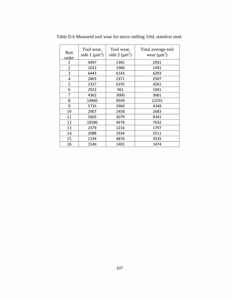
107

Table D.6 Measured tool wear for micro milling 316L stainless steel.

Run

order

number

Tool wear,

side 1 (µm3)

Tool wear,

side 2 (µm3)

Total average tool

wear (µm3)

1 4497 1365 2931

2 1023 1960 1491

3 6443 6143 6293

4 2803 2371 2587

5 2327 6195 4261

6 2922 961 1941

7 4362 3000 3681

8 14960 9549 12255

9 5735 2960 4348

10 2907 2458 2683

11 5603 3079 4341

12 10586 4678 7632

13 2379 1216 1797

14 2088 2934 2511

15 2194 4876 3535

16 1546 1402 1474

108

APPENDIX E

R STATISTICAL DATA

Figure E.1. Final model using R statistical software for meso milling A36 carbon steel.

Figure E.2. Residual plot for meso milling A36 carbon steel.

109

Figure E.3. Residuals vs Fitted for meso milling A36 carbon steel.

Figure E.4. Normal Q-Q plot for meso milling A36 carbon steel.

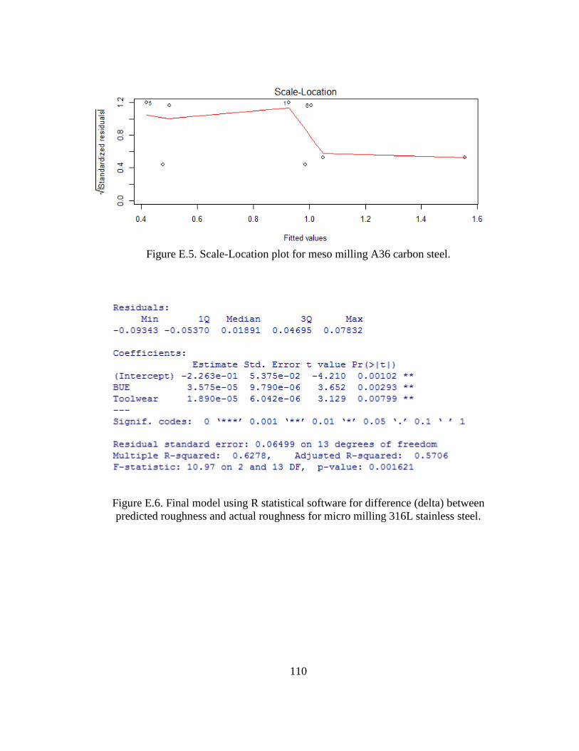
110

Figure E.5. Scale-Location plot for meso milling A36 carbon steel.

Figure E.6. Final model using R statistical software for difference (delta) between

predicted roughness and actual roughness for micro milling 316L stainless steel.

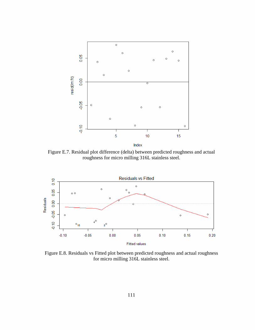
111

Figure E.7. Residual plot difference (delta) between predicted roughness and actual

roughness for micro milling 316L stainless steel.

Figure E.8. Residuals vs Fitted plot between predicted roughness and actual roughness

for micro milling 316L stainless steel.

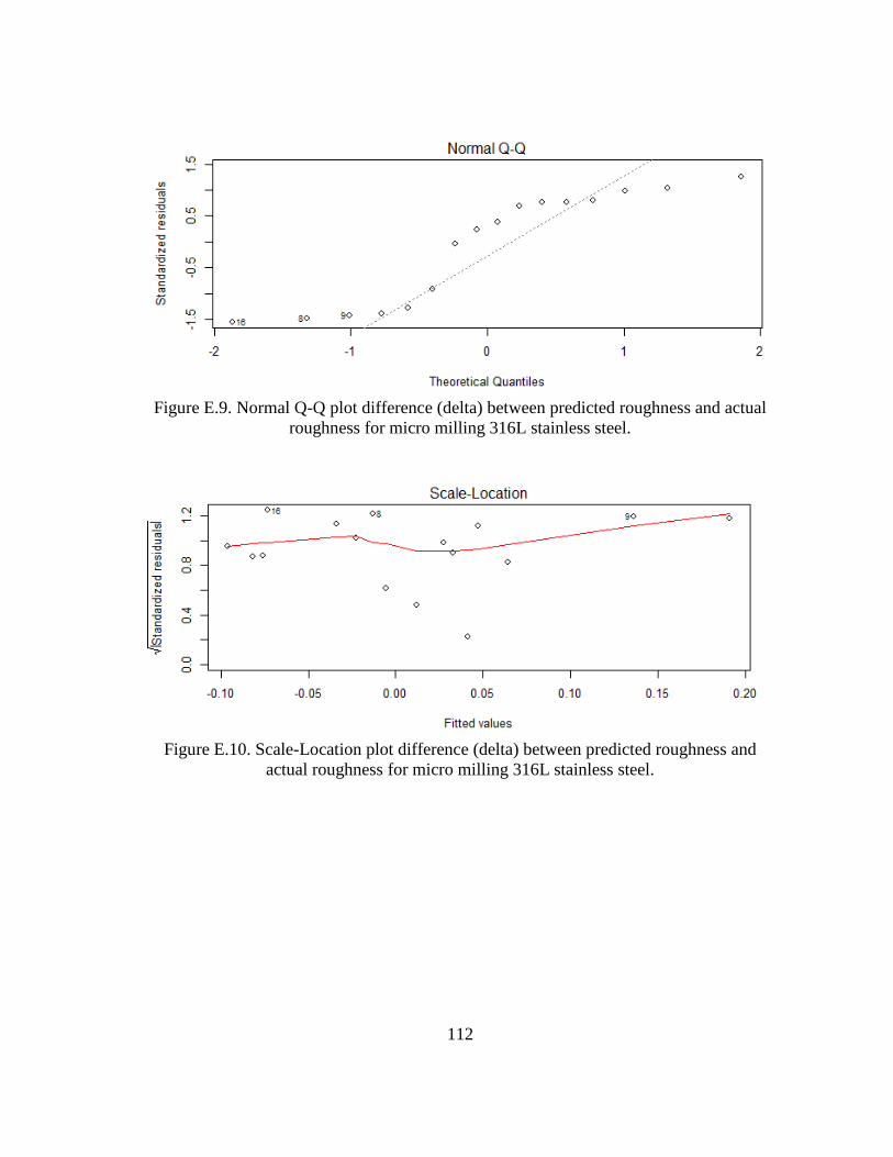
112

Figure E.9. Normal Q-Q plot difference (delta) between predicted roughness and actual

roughness for micro milling 316L stainless steel.

Figure E.10. Scale-Location plot difference (delta) between predicted roughness and

actual roughness for micro milling 316L stainless steel.

113

Figure E.11. Residuals vs Leverage plot difference (delta) between predicted roughness

and actual roughness for micro milling 316L stainless steel.

Figure E.12. Final model using R statistical software for BUE density for micro

milling 316L stainless steel.

114

Figure E.13. Residual plot using R statistical software for BUE density for micro milling

316L stainless steel.

Figure E.14. Residuals vs Fitted plot using R statistical software for BUE density for

micro milling 316L stainless steel.

115

Figure E.15. Normal Q-Q plot using R statistical software for BUE density for micro

milling 316L stainless steel.

Figure E.16. Scale-Location plot using R statistical software for BUE density for


116

Figure E.17. Residuals vs Leverage plot using R statistical software for BUE density for


Experimental Study of Built-up-edge Formation in Micro Milling

Documents

Transcript of Experimental Study of Built-up-edge Formation in Micro Milling