Experimental Investigation of Cavitation Induced … Institute of Aeronautics and Astronautics 1...

American Institute of Aeronautics and Astronautics

1

Exper imental Investigation of Cavitation Induced Feedline Instability from an O rifice

Matthew A. Hitt1 and David M. Lineberry2 University of Alabama in Huntsville, Huntsville, AL, 35899

Vineet Ahuja3 Combustion Research and F low Technology, Inc., Pipersvil le, PA, 18947

and

Robert A. Frederick4 University of Alabama in Huntsville, Huntsville, AL, 35899

This paper details the results of an exper imental investigation into the cavitation instabilities created by a ci rcular orifice conducted at the University of A labama in Huntsville Propulsion Research Center . This exper iment was conducted in concert with a computational simulation to serve as a reference point for the simulation. Testing was conducted using liquid nitrogen as a cryogenic propellant simulant. A 1.06 cm diameter thin orifice with a rounded inlet was tested in an approximately 1.25 kg/s flow with inlet pressures ranging from 504.1 kPa to 829.3 kPa. Pressure fluctuations generated by the orifice were measured using a high frequency pressure sensor located 0.64 tube diameters downstream of the orifice. Fast Fourier T ransforms were performed on the high frequency data to determine the instability frequency. Shedding resulted in a primary frequency with a cavitation related subharmonic frequency. For this exper iment, the cavitation instability ranged from 153 Hz to 275 Hz. Additionally, the strength of the cavitation occurred as a function of cavitation number . A t lower cavitation numbers, the strength of the cavitation instability ranged from 2.4 % to 7 % of the inlet pressure. However , at higher cavitation numbers, the strength of the cavitation instability ranged from 0.6 % to 1 % of the inlet pressure.

Nomenclature B = Systematic expanded uncertainty = Venturi beta ratio

Cd = Venturi discharge coefficient D = Tube inner diameter dv = Venturi throat diameter f = Frequency LN2 = Liquid nitrogen m = Mass flow rate = Dynamic viscosity

P = Pressure Pv = Vapor pressure Re = Reynolds number = Density

1Research Associate, UAHuntsville Propulsion Research Center, TH S225, AIAA Student Member 2Research Engineer, UAHuntsville Propulsion Research Center, TH S225, AIAA Senior Member 3Senio 4Professor/Interim Director, UAHuntsville Propulsion Research Center, TH S225, AIAA Associate Fellow

https://ntrs.nasa.gov/search.jsp?R=20130001791 2018-05-18T00:25:01+00:00Z


2

= Cavitation number St = Strouhal number t = Orifice thickness U = Expanded uncertainty V = Velocity Subscripts 1 = Orifice inlet vent = Venturi

I . Introduction HE occurrence of cavitation in a system can be detrimental to the performance or to the structural integrity of a rocket engine. As such, engines and feedlines are designed to minimize the impact of cavitation in the system.

To do this, an understanding of the nature and causes of cavitation is required. This can be done by testing simpler designs and conditions. The results of these experiments can then be used to construct computational models to describe the occurrence of cavitation in the component. These models can then be used to predict the occurrence and severity of cavitation in other components. This process can reduce the cost and time required to eliminate cavitation in a system.

As part of this objective, experimental testing was performed at the University of Alabama in Huntsville (UAHuntsville) Propulsion Research Center (PRC). The purpose of the experiment was to quantify the instabilities induced by the use of a cryogen through a rounded-inlet, circular orifice. The particular test conditions were selected to provide an experimental comparison for a CFD model. Multiple tests were conducted at the same mass flow rate and Reynolds number but with a variable orifice inlet pressure resulting in a variety of test conditions.

I I . Background Orifices are used in several different fluid applications including rocket propulsion systems. They are frequently

used to control the mass flow rate in a system, reduce the pressure in a system, or to dampen pressure oscillations in a system.1-3 However, orifices are particularly vulnerable to cavitation due to the high jet velocities at the orifice throat.2 As the flow cavitates in the orifice, pressure feed system instabilities can be generated which can be detrimental to the feed system and lead to reduced engine performance.

In launch vehicles, low frequency feed system instabilities can couple with the natural harmonics of the launch vehicle leading to a pogo instability in the vehicle. This coupling leads to the expansion and contraction of the vehicle. These instabilities can be caused by different components in a system. Pogo instabilities caused by cavitation at the oxygen and fuel pump inlets were seen in the Titan II rocket.4 Cavitation induced instabilities in launch vehicle feed systems can lead to thrust oscillations. Due to the lower density and high volume of cavitation bubbles, the mass flow rate downstream of the cavitation point can fluctuate. Since thrust is a function of the propellant flow rates, the mass flow rate oscillations lead to thrust oscillations in the engine.5

The presence of cavitation in feed system components is eliminated as much as possible in order to avoid the negative effects it can have on a vehicle performance. To better remove cavitation in a feedline system, computational models are developed to predict the existence of cavitation and determine means of eliminating it. In order to improve the effectiveness of the computational models, experimental tests are conducted to validate the results from the models.

A . Combustion Instability Combustion instability is when significant pressure oscillations occur in the combustion chamber of an engine.

These instabilities may or may not be detrimental to the engine. In general, combustion instability can be divided into three different categories depending upon the frequency range and source of the instability as shown in Table 1..

T

Table 1. Combustion Instability Modes3 Instability Frequency CauseChugging < 400 Hz Feedline

BuzzingFeedline or Combustion

Acoustic > 1000 Hz Combustion


3

instability is typically generated by oscillations created by feed system components. While this type does not typically couple with the combustion chamber, large volume combustion chambers with low frequency responses can couple with chugging instability. While not strictly combustion instability, a chugging instability can couple with t , as described above. . Chugging instabilities typically do not result in engine damage . However, chugging instabilities reduce engine efficiency and create thrust oscillations.

Hz. Buzzing instability can be generated by either feedline or combustion chamber instabilities. As such, buzzing instabilities are often better considered as higher frequency chugging instabilities or lower frequency acoustic instabilities rather than their own class of instability. As with chugging instabilities, buzzing instabilities tend to be less damaging to the launch vehicle than acoustic instabilities.3, 6

High frequency instabilities, also known as acoustic instabilities, are are considered to occur above 1000 Hz. Acoustic instabilities are typically generated by combustion phenomena and not by feedline instabilities.

B . Cavitation The formation and collapse of bubbles in a flowing liquid is called cavitation.7 Cavitation occurs when the

velocity of a liquid causes the local static pressure to drop below the local vapor pressure. Some studies have also indicated that viscous shear stresses can influence the formation of cavitation.8 In rocket engines, the necessary velocities, and resulting shear stresses and pressure drops, for cavitation can be easily produced by an orifice2. When the velocity reaches levels capable of producing cavitation, a vapor cavity starts to grow on a solid surface in contact with the liquid.8 As the vapor cavity grows, the cavity starts to elongate into the system, and disturbances in the system cause the cavity to split forming a vapor bubble.10 The bubble travels downstream until it reaches a point in the flow where the local static pressure returns above the vapor pressure. When the bubble reaches a high pressure point, the bubble collapses. While cryogens follow the same pattern in cavitation development as other liquids, cryogenic liquids form smaller bubbles than other liquids due to thermodynamic effects from vaporization.5 As the cryogen vaporizes, a thermal depression is created in the flow which reduces the size of the bubble because more energy is required to form a bubble in a colder area.5

To characterize the type and severity of the cavitation in a system, a nondimensional cavitation number is used. It should be noted that cavitation number can be defined in different manners depending on the application . Due to the type of component tested and the location of the sensors, the cavitation number used in this experiment is defined by the classical fluid dynamics relation,

2

1

21

orif

v

V

PP (1)

here P1 is the upstream pressure, Pv is the vapor pressure based on the temperature at the P1 1 measurement location, and Vorif is the velocity at the orifice throat. The cavitation number represents the pressure drop required to induce cavitation relative to the dynamic pressure induced through the orifice. and indicates the relative strength of cavitation at the test point. As the cavitation number decreases, the relative strength of the cavitation increases.7, 11-12

Cavitation in a system generally occurs in two main types; when cavitation first begins to occur in the system. During incipient cavitation, the flow rate of the fluid still increases with increasing pressure drop. As cavitation continues to develop, it eventually reaches the point termed choked cavitation. Once choked cavitation occurs, the volumetric flow rate of the fluid through the component becomes fixed and no longer increases with increasing pressure drop.7 Typically, incipient cavitation occurs at a cavitation number on the order of 1.11 However, in some cases, cavitation has been observed to occur at a higher cavitation number than 1.12

Cavitation in a system can have several negative effects in the system. These effects range from minor difficulties such as increased noise level to damage of system components. When the cavitation bubbles reach a region of higher pressure, they collapse violently. This violent collapse can create significant localized pressure spikes. These bubble implosions and pressure spikes can cause erosion and damage of components in the system as

erosion is particularly serious if the bubbles collapse next to the surface of a component. Erosion of a system component can lead to structural fatigue and failure or can remove protective coatings from the component resulting in potential corrosion damage.7, 9, 13 In addition to system damage, cavitation can cause an efficiency loss in a system. As the system


4

cavitates, the local fluid density fluctuates due to the lower density of vapor and the high volume of the bubbles produced. These fluctuations in the fluid density cause the mass flow rate in the system to fluctuate. This in turn can result in a thrust fluctuations and pogo instabilities discussed previously.

Cavitation has had negative effects on actual launch vehicles. Specifically, cavitation instabilities in the Delta 4 oxidizer feed line are considered to have been contributory to erroneous pressure readings leading to an early shutdown of the RS-68 engine.14 Also, large pressure fluctuations have contributed to structural cracks in the liquid hydrogen lines in the space shuttle.14

C . O rifice F low In addition to cavitation instabilities, the use of an orifice in a flow can also result in additional fluid dynamic

instabilities. These instabilities can result from such phenomena as turbulence or vortex shedding.14 One significant example of fluid dynamic instability is orifice whistling. Orifice whistling occurs when the acoustic power scattered from an orifice is greater than the power incident to the orifice. To estimate at what frequency the orifice whistling will occur, the Strouhal number is used. The Strouhal number is defined as

1V

tfSt (2)

where St is the Strouhal number, f is the orifice shedding frequency, t is the orifice thickness, and V1 is the orifice throat velocity. The Strouhal number is a function of Reynolds number and generally lies in the range of 0.2 to 0.3.15-17 If whistling occurs in an orifice, acoustic feedback can occur and cause instabilities to exist upstream of the orifice.11

I I I . Exper imental Approach To evaluate the cavitation instabilities created by an orifice, a test system was developed for using LN2. The

system was equipped with thermocouples and static pressure transducers to characterize the flow conditions. A high frequency pressure sensor was used to measure the frequency and amplitude of the instabilities downstream of the orifice. To determine the effect of the cavitation related instabilities, a test matrix was planned to test at conditions with a stronger cavitation response and at conditions with a weaker cavitation response.

A . PR C C ryogenic Test Facility Testing for the project was conducted at the University of Alabama in Huntsville (UAH) Propulsion Research

Center (PRC) using the PRC Cryogenic Test Facility.18 The PRC cryogenic test facility was originally designed to deliver single phase liquid oxygen to a rocket hot-fire test stand at flow rates of up to 1.36 kg/s (3 lbm/s). The facility is capable of handling inert or oxidizing cryogenic liquids in the temperature range of atmospheric LN2 or warmer. The facility was modified from the hot-fire rocket testing configuration in order to better accommodate the LN2 flow testing conducted in this experiment. The revised flow path consisted of 2.54 cm (1 in.) OD tubing without teflon nitrogen jacket. The existing 1.27 cm (0.5 in.) valves and fittings were replaced with 2.54 cm (1 in.) components or eliminated where possible. The overall flow path length from the run tank to the test article was shortened and simplified as much as possible to minimize heat losses and pressure losses through the system. These changes allowed for testing at an increased flow rate while maintaining a lower operating pressure in order to allow for cavitation in the test orifice without having cavitation occur in the system.

The flow path for the orifice testing consisted of 2.54 cm (1 in.) outer diameter 316 stainless steel tubing with 0.21 cm (0.083 in.) wall thickness resulting in a 2.12 cm (0.834 in.) inner diameter flow path. The tubing and components in the system were insulated using Cryogel®Z insulation to minimize the heat transfer from the surroundings into the LN2. The flow through the system was initiated by opening a manually actuated, quarter turn, cryogenic ball valve. The mass flow rate was controlled by a fixed diameter, cavitating venturi. The governing equation used for calculating the flow rate was

42

1)(2

)4

( ven tvven tvd

ppdCm (3)

where m is the mass flow rate, Cd is the discharge coefficient, dv is the throat diameter of the venturi, p1 is the venturi inlet pressure, pvent vent is the density of the LN2 is the ratio of the venturi throat diameter to the tubing inner diameter. The discharge coefficient was determined from manufacturer data using the manufacturer specified mass flow rate and fluid properties.


5

The inlet pressure of the test orifice was controlled using a cryogenic globe valve downstream of the test orifice. Once mass flow rate was set through the cavitating venturi, the test orifice inlet pressure was controlled by adjusting the position of the throttle valve. As the valve was closed, the pressure drop across the valve increased thus increasing the orifice inlet and outlet pressures for a fixed mass flow, After the backpressure valve, the flowpath expanded to 1-1/2 in. copper pipe and was plumbed into the test stand oxygen vent and vented to atmosphere.

The test orifice used in this experiment was a single element, circular orifice. The orifice had a throat diameter of 1.06 cm (0.417 in.) and a beta ratio of 0.5. The test orifice had a smooth inlet with a 0.26 cm (0.104 in.) radius and was 0.53 cm (0.209 in.) thick. This thickness yields a thickness to diameter ratio of 0.5 which falls within the range for a thin orifice.11 The test orifice component was fabricated from 316 stainless steel. In addition to the orifice, the component included a high frequency measurement port 1.32 cm (0.521 in. or 0.625 tubing diameters) downstream of the orifice. Tube fittings were welded using smooth welds to the component to connect the component to the flow path. A picture of the flow path is shown in Fig. 1.

B . Instrumentation and Uncertainty Temperature measurements were taken upstream of the main ball valve, upstream of the cavitating venturi,

upstream of the orifice and downstream of the orifice. Each location had an Omega TMQSS-125U-6 T-type thermocouple. The thermocouples were not calibrated on site for the temperature range expected in testing, thus the uncertainty for the thermocouples was taken as the larger of 1.0 °C or 1.5% of measurement, as per the manufacturer specifications.

In addition to system static pressure measurements necessary for establishing flow from the run tank, static pressure measurements were taken upstream of the venturi and upstream and downstream of the orifice. These static pressure measurements were made using Omega pressure transducers. Each of the static pressure transducers used a 0.32 cm (0.125 in.) OD tubing standoff which positioned the transducer approximately 76.2 cm (30 in.) away from the main tubing to protect the transducers from the cryogenic temperatures. Each static pressure transducer was connected to the DAQ and calibrated over the range 0 to 1965 kPa (0 to 285 psig) using a deadweight pressure tester. The transducers were assumed to have a linear pressure-voltage relationship and a 2nd order regression analysis was performed to determine calibration uncertainty for each transducer.19

A single high frequency dynamic pressure measurement was taken downstream of the orifice to measure pressure fluctuations resulting from flow instabilities. The measurement was made using a PCB 112A05 pressure sensor with a PCB 422E51 in-line charge converter. The pressure sensor had a minimum operating temperature of -

LN2 Run Tank

Manual Ball Valve

Cavitating Venturi

Test Article

Back Pressure Throttle Valve

F igure 1. C ryogenic Test Facility


6

240 °C and a sensitivity of 1.1 pC/psi. The inline charge converter had a 100 mV/pC conversion factor and a ±5 V output. The pressure sensor and charge converter combination had a ±296.5 kPa (±43 psi) output.

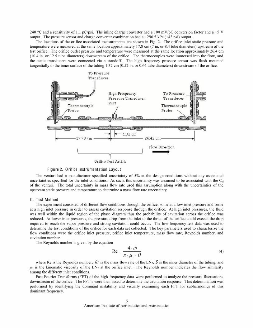
The locations of the orifice associated measurements are shown in Fig. 2. The orifice inlet static pressure and temperature were measured at the same location approximately 17.8 cm (7 in. or 8.4 tube diameters) upstream of the test orifice. The orifice outlet pressure and temperature were measured at the same location approximately 26.4 cm (10.4 in. or 12.5 tube diameters) downstream of the orifice. The thermocouples were immersed into the flow, and the static transducers were connected via a standoff. The high frequency pressure sensor was flush mounted tangentially to the inner surface of the tubing 1.32 cm (0.52 in. or 0.64 tube diameters) downstream of the orifice.

The venturi had a manufacturer specified uncertainty of 5% at the design conditions without any associated

uncertainties specified for the inlet conditions. As such, this uncertainty was assumed to be associated with the Cd of the venturi. The total uncertainty in mass flow rate used this assumption along with the uncertainties of the upstream static pressure and temperature to determine a mass flow rate uncertainty.

C . Test M ethod The experiment consisted of different flow conditions through the orifice, some at a low inlet pressure and some

at a high inlet pressure in order to assess cavitation response through the orifice. At high inlet pressures, the fluid was well within the liquid region of the phase diagram thus the probability of cavitation across the orifice was reduced. At lower inlet pressures, the pressure drop from the inlet to the throat of the orifice could exceed the drop required to reach the vapor pressure and strong cavitation could occur. The low frequency test data was used to determine the test conditions of the orifice for each data set collected. The key parameters used to characterize the flow conditions were the orifice inlet pressure, orifice inlet temperature, mass flow rate, Reynolds number, and cavitation number.

The Reynolds number is given by the equation

D

m

1

4Re (4)

where Re is the Reynolds number, m is the mass flow rate of the LN2, D is the inner diameter of the tubing, and 1 is the kinematic viscosity of the LN2 at the orifice inlet. The Reynolds number indicates the flow similarity

among the different inlet conditions. Fast Fourier Transforms (FFT) of the high frequency data were performed to analyze the pressure fluctuations

assed to determine the cavitation response. This determination was performed by identifying the dominant instability and visually examining each FFT for subharmonics of this dominant frequency.

F igure 2. O rifice Instrumentation Layout


7

I V . Results The orifice testing was conducted in seven different test runs. Data was continuously recorded throughout each

run. These data included start-up and shut-down data as well as data during back pressure throttling. From the data, sets of measurements were taken for steady state inlet conditions only. Transient data sets were neglected from the analysis. In addition, the inlet condition data sets were analyzed, and the average cavitation number for each set of data were calculated. To focus on the effect of cavitation, the data sets with cavitation numbers in the range of 0.5 to 2.5 were selected. Finally, an FFT was performed for each set of test data, and the maximum amplitude and the associated frequency were determined. To remove the effect of a non-zero mean in the pressure data, the first two FFT bins were set equal to zero. The FFT results were then examined, and the data from several operating conditions were noticed to have strong instantaneous pressure spikes which resulted in inaccurate FFT results. These data sets and graphs are not analyzed here. These criteria resulted in 15 data sets for the orifice testing. The following sections detail the results of a representative test condtition and provide a summary of all the test points.

A . Test Results Overview The summary of the average orifice and venturi conditions with uncertainty for the data sets are shown in Table

12. Results from the test data show that the orifice inlet pressure ranged from 601.2 kPa (87.2 psia) to 829.5 kPa (120.3 psia). While the uncertainty for a few data sets slightly extended into the vapor regime, the inlet conditions for each of the data sets were on the liquid side of the vapor curve.

The temperature and pressure data were used to calculate the mass flow rate, pressure drop, Reynolds number, cavitation number, and Strouhal number. The results of these calculations are shown inTable 3. An important note regarding the uncertainties provided in this table is that the cavitation number uncertainty is presented as the absolute value while the other uncertainties provided are percentages of the nominal value. This presentation was selected due to the small values of the cavitation number.

The inlet conditions were non-dimensionalized using the cavitation number for comparison. The cavitation number data show two distinct groupings. One group had cavitation numbers ranging from 0.6 to 1.1, and another group had cavitation numbers ranging from 2.1 to 2.5. The mass flow rate was relatively constant over the all of the data sets with average flow rates ranging from 1.22 kg/s to 1.29 kg/s (2.69 lbm/s to 2.83 lbm/s) with approximately 8 % uncertainty. The pressure drop across the orifice was also fairly constant with an approximate value of 103.4 kPa (15 psid) for all the data sets. The average Reynolds number ranged from 789,300 to 833,800 with 11 % to 12 % uncertainty. These Reynolds numbers indicate that the flow was fully turbulent for all data sets. The relative constancy of these parameters indicates that the inlet flow conditions for each data set were similar. The Strouhal numbers all fell within the expected range of 0.2 to 0.3. This range is consistent for the wake frequencies identified from the data set FFT

Table 2. Testing Conditions Summary

Test Set [kPa]Uncertainty

[%] [K]Uncertainty

[%] [kPa]Uncertainty

[%] [K]Uncertainty


[%] [K]Uncertainty

[%]164499 103 1682.9 0.5 93.1 2.9 617.0 2.5 94.7 2.8 516.6 3.0 109.4 2.2165099 33 1640.7 0.5 90.5 3.0 601.2 2.6 92.2 2.9 498.1 3.2 107.2 2.3165099 34 1637.4 0.5 90.4 3.0 601.2 2.6 92.2 2.9 499.3 3.2 107.3 2.3166178 41 1665.0 0.5 93.6 2.9 650.5 2.3 94.9 2.8 551.3 2.8 109.6 2.2166178 42 1662.5 0.5 93.6 2.9 649.0 2.3 95.0 2.8 550.4 2.8 109.7 2.2166178 43 1660.7 0.5 93.6 2.9 649.1 2.3 95.0 2.8 550.4 2.8 109.7 2.2167223 39 1673.3 0.5 92.2 2.9 634.8 2.4 93.8 2.9 530.2 3.0 108.6 2.3167223 41 1668.0 0.5 92.2 2.9 829.3 1.8 93.4 2.9 721.0 2.1 108.9 2.3167223 42 1665.1 0.5 92.2 2.9 826.6 1.8 93.4 2.9 718.8 2.1 108.9 2.3167223 43 1662.2 0.5 92.3 2.9 824.1 1.8 93.4 2.9 715.8 2.1 108.8 2.3167223 44 1659.5 0.5 92.3 2.9 824.2 1.8 93.3 2.9 715.8 2.1 108.7 2.3167223 54 1632.7 0.5 92.4 2.9 765.0 1.9 93.3 2.9 660.4 2.3 108.6 2.3167223 55 1630.7 0.5 92.4 2.9 766.4 1.9 93.2 2.9 662.7 2.3 108.5 2.3167223 56 1628.7 0.5 92.4 2.9 765.6 1.9 93.2 2.9 662.1 2.3 108.6 2.3167223 59 1621.6 0.5 92.9 2.9 650.8 2.3 94.0 2.9 551.6 2.8 108.8 2.3

Inlet Temp Outlet Pressure Outlet TempVenturi Pressure Venturi Temp Inlet Pressure


8

B . Sample H igh F requency Data The high frequency test data from Test 165099-Set 33 are shown in Figure 3. A magnified section of these data

is shown in Figure 4. As can be seen in the plots, the data include several sharp spikes in the pressure trace. These spikes are likely due to the occurrence of cavitation in the flow. Since this data set had a cavitation number of 1.1, the presence of cavitation was expected. It should be noted that the pressure signal shows that at these strong spikes, the pressure exceeds the limits of the transducer resulting in saturation. For the high frequency pressure sensor and charge converter used in this experiment, saturation occurred when the pressure spikes exceeded ±296.5 kPa (±43 psi). Saturation of the transducer was exacerbated due to the fluctuations of the dynamic transducer resulting in a non-zero mean. For a saturated signal, the absolute magnitudes of the instability peaks are not reliable. However, the qualitative strengths of the peaks may be compared. When saturation occurs in a measurement, the measured signal appears as a square wave. As such, when an FFT is conducted for a saturated sensor, harmonics of the frequency can appear.

F igure 3. Test 165099-Set 33 H igh F requency Raw Signal

Table 3. Test Conditions Results

Test Set [kg/s]Uncertainty


% UncertaintyUncertainty

%Uncertainty

%164499 103 1.25 8.1 100.3 0.2 0.6 0.8 833800 12 0.24 10165099 33 1.29 7.7 103.1 0.2 1.1 0.7 795800 11 0.28 10165099 34 1.29 7.7 101.9 0.2 1.1 0.7 795300 11 0.29 10166178 41 1.23 8.3 99.2 0.2 0.8 0.8 825900 12 0.27 11166178 42 1.23 8.3 98.5 0.3 0.8 0.9 826100 12 0.27 10166178 43 1.23 8.3 98.7 0.3 0.8 0.9 825500 12 0.27 11167223 39 1.26 8.0 104.6 0.2 1.0 0.8 820200 11 0.27 10167223 41 1.26 8.0 108.3 0.4 2.5 0.9 810200 12 0.27 10167223 42 1.26 8.0 107.8 0.5 2.4 0.9 809000 12 0.22 10167223 43 1.26 8.0 108.3 0.5 2.4 0.9 807200 12 0.27 10167223 44 1.26 8.0 108.4 0.4 2.5 0.9 804900 12 0.26 10167223 54 1.24 8.1 104.6 0.4 2.1 0.9 792500 12 0.21 10167223 55 1.24 8.1 103.7 0.3 2.1 0.9 790000 12 0.20 10167223 56 1.24 8.1 103.5 0.3 2.1 0.9 789300 12 0.21 10167223 59 1.22 8.2 99.2 0.3 1.1 0.8 799700 12 0.27 10

Mass Flow Rate Orifice Pressure Drop Cavitation Number Reynold's Number Strouhal Number


9

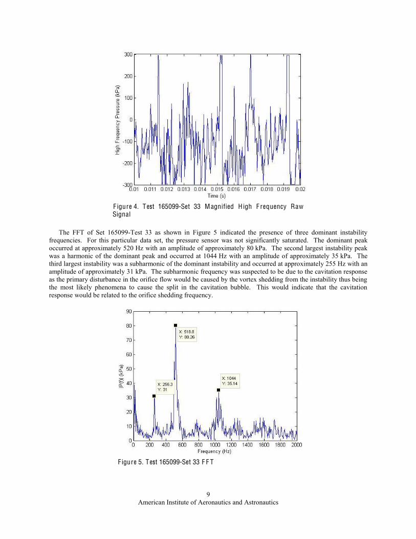
The FFT of Set 165099-Test 33 as shown in Figure 5 indicated the presence of three dominant instability frequencies. For this particular data set, the pressure sensor was not significantly saturated. The dominant peak occurred at approximately 520 Hz with an amplitude of approximately 80 kPa. The second largest instability peak was a harmonic of the dominant peak and occurred at 1044 Hz with an amplitude of approximately 35 kPa. The third largest instability was a subharmonic of the dominant instability and occurred at approximately 255 Hz with an amplitude of approximately 31 kPa. The subharmonic frequency was suspected to be due to the cavitation response as the primary disturbance in the orifice flow would be caused by the vortex shedding from the instability thus being the most likely phenomena to cause the split in the cavitation bubble. This would indicate that the cavitation response would be related to the orifice shedding frequency.

F igure 5. Test 165099-Set 33 F F T

F igure 4. Test 165099-Set 33 Magnified H igh F requency Raw Signal


10

C . Instability Analysis For this analysis, the three strongest instabilities were categorized as the primary instability, the subharmonic

instability, and the harmonic instability. The primary instability typically had the largest amplitude and was typically in the range of 400 to 500 Hz. The harmonic instability was hypothesized to be a product of the wake instability caused by the whistling of the orifice. A Strouhal number was calculated using the harmonic instability frequency as the sheding frequency in the Strouhal equation. For the previously mentioned sample point, this gave a Strouhal number of 0.28 ± 10 % which falls within the expected range of 0.2 to 0.3. The primary instability was considered to be a result of the same shedding phenomena that caused the harmonic instability. The high frequency pressure measurements were made only on one side of the tubing. Because of the helical nature of vortex shedding from a circular orifice, the pressure sensor would be more strongly influenced by vortices near the sensor than those on the opposite side of the tubing leading to a measured frequency equal to roughly ½ of the shedding frequency. The subharmonic instability is the instability considered to be primarily produced from cavitation. This frequency is less than the primary frequency because not all vortices will contain cavitation bubbles. The three instabilities for each data set are shown in Table 4.

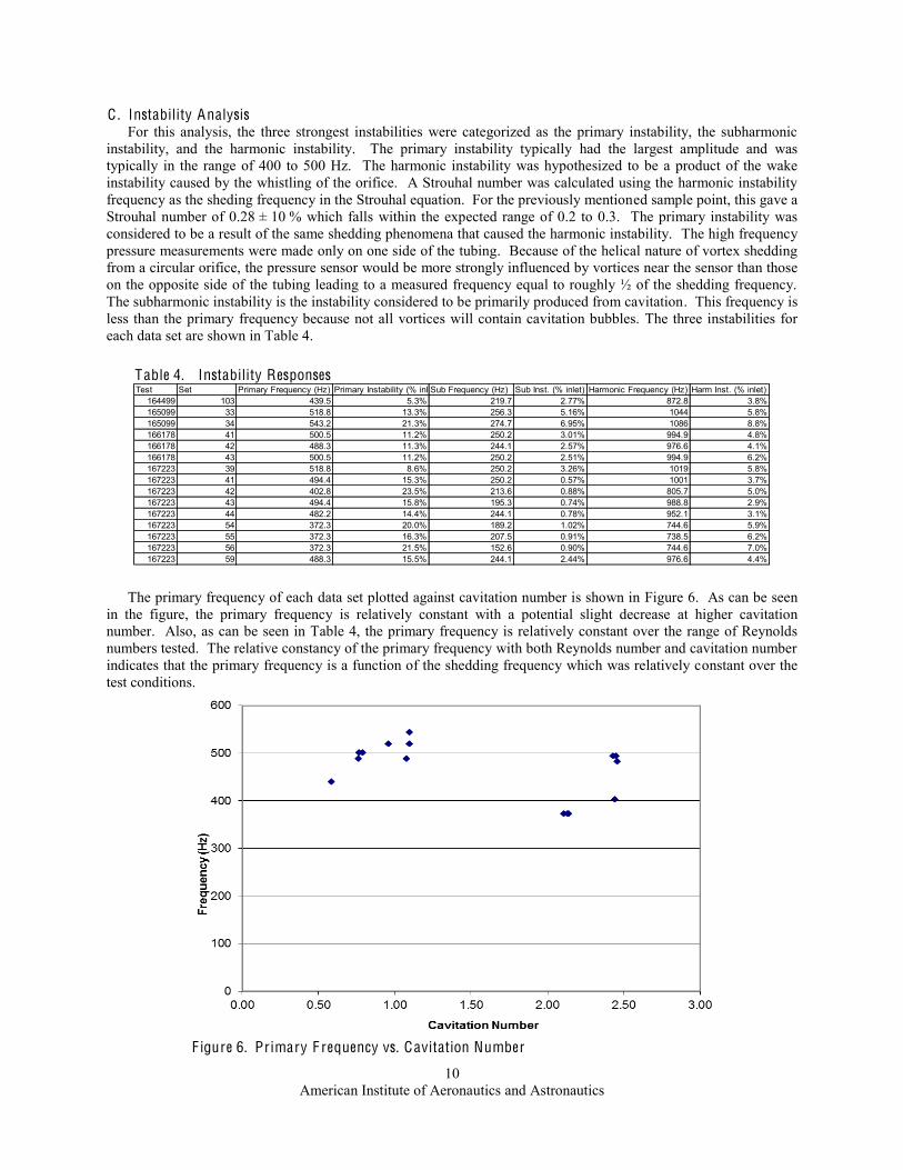
The primary frequency of each data set plotted against cavitation number is shown in Figure 6. As can be seen in the figure, the primary frequency is relatively constant with a potential slight decrease at higher cavitation number. Also, as can be seen in Table 4, the primary frequency is relatively constant over the range of Reynolds numbers tested. The relative constancy of the primary frequency with both Reynolds number and cavitation number indicates that the primary frequency is a function of the shedding frequency which was relatively constant over the test conditions.

F igure 6. Primary F requency vs. Cavitation Number

Table 4. Instability Responses Test Set Primary Frequency (Hz) Primary Instability (% inlet)Sub Frequency (Hz) Sub Inst. (% inlet) Harmonic Frequency (Hz) Harm Inst. (% inlet)

164499 103 439.5 5.3% 219.7 2.77% 872.8 3.8%165099 33 518.8 13.3% 256.3 5.16% 1044 5.8%165099 34 543.2 21.3% 274.7 6.95% 1086 8.8%166178 41 500.5 11.2% 250.2 3.01% 994.9 4.8%166178 42 488.3 11.3% 244.1 2.57% 976.6 4.1%166178 43 500.5 11.2% 250.2 2.51% 994.9 6.2%167223 39 518.8 8.6% 250.2 3.26% 1019 5.8%167223 41 494.4 15.3% 250.2 0.57% 1001 3.7%167223 42 402.8 23.5% 213.6 0.88% 805.7 5.0%167223 43 494.4 15.8% 195.3 0.74% 988.8 2.9%167223 44 482.2 14.4% 244.1 0.78% 952.1 3.1%167223 54 372.3 20.0% 189.2 1.02% 744.6 5.9%167223 55 372.3 16.3% 207.5 0.91% 738.5 6.2%167223 56 372.3 21.5% 152.6 0.90% 744.6 7.0%167223 59 488.3 15.5% 244.1 2.44% 976.6 4.4%


11

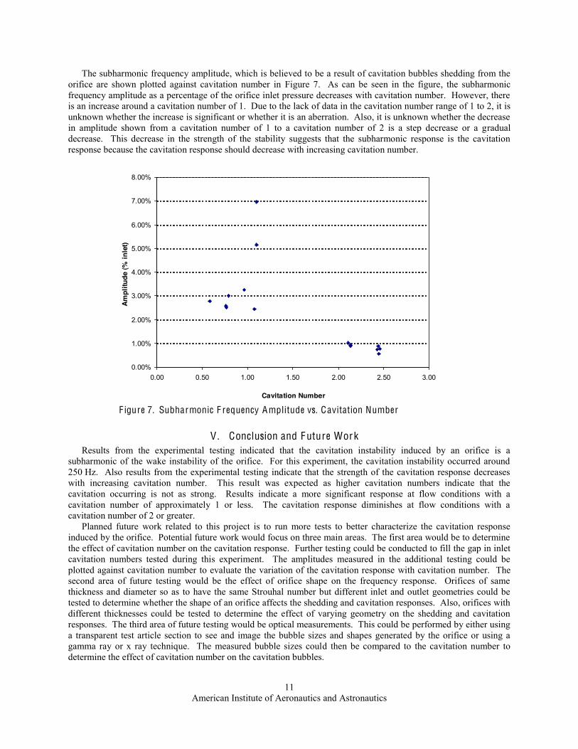
The subharmonic frequency amplitude, which is believed to be a result of cavitation bubbles shedding from the orifice are shown plotted against cavitation number in Figure 7. As can be seen in the figure, the subharmonic frequency amplitude as a percentage of the orifice inlet pressure decreases with cavitation number. However, there is an increase around a cavitation number of 1. Due to the lack of data in the cavitation number range of 1 to 2, it is unknown whether the increase is significant or whether it is an aberration. Also, it is unknown whether the decrease in amplitude shown from a cavitation number of 1 to a cavitation number of 2 is a step decrease or a gradual decrease. This decrease in the strength of the stability suggests that the subharmonic response is the cavitation response because the cavitation response should decrease with increasing cavitation number.

V . Conclusion and Future Work Results from the experimental testing indicated that the cavitation instability induced by an orifice is a

subharmonic of the wake instability of the orifice. For this experiment, the cavitation instability occurred around 250 Hz. Also results from the experimental testing indicate that the strength of the cavitation response decreases with increasing cavitation number. This result was expected as higher cavitation numbers indicate that the cavitation occurring is not as strong. Results indicate a more significant response at flow conditions with a cavitation number of approximately 1 or less. The cavitation response diminishes at flow conditions with a cavitation number of 2 or greater.

Planned future work related to this project is to run more tests to better characterize the cavitation response induced by the orifice. Potential future work would focus on three main areas. The first area would be to determine the effect of cavitation number on the cavitation response. Further testing could be conducted to fill the gap in inlet cavitation numbers tested during this experiment. The amplitudes measured in the additional testing could be plotted against cavitation number to evaluate the variation of the cavitation response with cavitation number. The second area of future testing would be the effect of orifice shape on the frequency response. Orifices of same thickness and diameter so as to have the same Strouhal number but different inlet and outlet geometries could be tested to determine whether the shape of an orifice affects the shedding and cavitation responses. Also, orifices with different thicknesses could be tested to determine the effect of varying geometry on the shedding and cavitation responses. The third area of future testing would be optical measurements. This could be performed by either using a transparent test article section to see and image the bubble sizes and shapes generated by the orifice or using a gamma ray or x ray technique. The measured bubble sizes could then be compared to the cavitation number to determine the effect of cavitation number on the cavitation bubbles.

0.00%

1.00%

2.00%

3.00%

4.00%

5.00%

6.00%

7.00%

8.00%

0.00 0.50 1.00 1.50 2.00 2.50 3.00

Cavitation Number

Ampl

itude

(% in

let)

F igure 7. Subharmonic F requency Amplitude vs. Cavitation Number


12

Acknowledgments The authors would like to thank the staff and students of the UAHuntsville Propulsion Research Center for their

support and encouragement during this study. M. A. Hitt thanks UAHuntsville for the support of the Von Braun Propulsion Scholarship. This research was supported by the NASA STTR Program. The Contract Monitor was Dr. Daniel Allgood.

References 1Broerman, E. L., Smol

-26246, 2007 ASME Pressure Vessels and Piping Division Conference, San Antonio, Texas, 22-26 July 2007.

2Adams, JCode to the Design of a Multi-Stage Breakdown Orifice in Support of GSI- -26208, 2007 ASME Pressure Vessels and Piping Division Conference, San Antonio, Texas, 22-26 July 2007.

3Sutton, G. P., and Biblarz, O., Rocket Propulsion Elements, 8th ed., John Wiley & Sons, Inc., Hoboken, New Jersey, 2010, Chap. 9, 11.

4 - Crosslink, Vol. 5, No. 1, 2003/2004, pp. 26-29. 5 Journal of Mechanical

Science and Technology, Vol. 23, No. 3, 2009, pp. 643-649. 6Harrje, D., and Reardon, F. (ed.), -194, 1972. 7Skousen, P.., Valve Handbook, 3rd ed., McGraw Hill, New York, 2011, Chap. 9. 8 Physics of F luids, Vol. 19, No. 7, 2007. 9White, F. M., F luid Mechanics, 6nd ed., McGraw Hill, New York, 2006. 10Stutz, B., and Reboud, J.- Experiments in F luids, Vol. 29, No. 6, 2000, pp.

545-552. 11Testud, P., Moussou, P., Hirschberg -hole and Multi-hole

Journal of F luids and Structures, Vol. 23, No. 2, 2007, pp. 163-189. 12 -2011-0808, 49th AIAA Aerospace Sciences Meeting

and Exhibit, Orlando, Florida, 4-7 January 2011. 13 Proc. O f 1st FPNI-PhD Symp., Hamburg, 2000, pp. 371-382. 14 -26639, 2007 ASME Pressure

Vessels and Piping Division Conference, San Antonio, Texas, 22-26 July 2007. 15

PVP2007-26157, 2007 ASME Pressure Vessels and Piping Division Conference, San Antonio, Texas, 22-26 July 2007. 16White, F. M., Viscous F luid F low, 3rd ed., McGraw Hill, New York, 2006, Chap. 1. 17 Validation of a Whistling Criterion for Orifices in Air Pipe

th French Congress of Acoustics, Tours, France, 24-27 April 2006. 18

Thesis, Mechanical and Aerospace Engineering Department, University of Alabama in Huntsville, Huntsville, AL, 2010. 19Coleman, H. W., and Steele, W. G., Experimentation, Validation, and Unceratinty Analysis for Engineers, 3rd ed., John

Wiley & Sons, Inc., Hoboken, New Jersey, 2009, Chap. 3-4.

Experimental Investigation of Cavitation Induced … Institute of Aeronautics and Astronautics 1...

Documents

Transcript of Experimental Investigation of Cavitation Induced … Institute of Aeronautics and Astronautics 1...