Experimental Investigation of Air-Sea Transfer of Momentum and Enthalpy at High Wind Speed

By: Moshe Alamaro1, Kerry A. Emanuel1, Wade R. McGillis2

1 Department of Earth, Atmospheric and Planetary Sciences, Massachusetts Institute of Technology; 2 Woods Holes Oceanographic Institution.

Abstract. Thermodynamic analysis and numerical modeling of hurricanes show that

their intensity is sensitive to enthalpy and momentum transfer from the ocean surface.

Since direct measurements of drag are not easily performed on the high seas, an

annular wind-wave tank was constructed to simulate some aspects of the tropical storm

boundary layer. The maximum air velocity inside the annular tank is comparable to that

of a hurricane.

This paper describes the design and engineering of the tank, the fluid mechanics of the

rotational flow in the tank using angular momentum analysis, the design of the

experiments, and experimental results. It provides experimental data on drag and latent

enthalpy transfer at high air speed relative to the moving water surface. The design of

the wind-wave tank and the experiments provide a foundation for future and more

comprehensive high air speed experimental programs using a linear tank.

Key Words: Air-sea interaction, spray, tropical cyclones, heat and momentum transfer.

1. Introduction

Basic theory (e.g., Emanuel 1986) and numerical experiments (Ooyama 1969;

Rosenthal 1971; Emanuel 1995a) show that the intensity of tropical cyclones depends

strongly on the coefficients for the transfers of momentum (CD) and enthalpy (Ck)

between the ocean and the atmospheric boundary layer. The maximum wind speed, in

particular, depends on (Ck /CD)1/2 in the high wind speed core of the storm (Emanuel

1986). Unfortunately, there are no simultaneous measurements of the effective values of

these coefficients at wind speeds greater than about 25 m s-1, and the theory of air–sea

interaction at very high wind speeds is poorly developed. The agitated sea no doubt

increases the effective roughness length and, thereby, CD and the dissipation rate of

kinetic energy; while, for wind speeds up to about 20 m s-1, there is little observational

evidence to suggest a corresponding increase in Ck (Geernaert et al. 1987). Emanuel

(1995a) showed that if estimated values of the exchange coefficients at 20 m s-1 are

applied at higher wind speeds, maintaining a storm of much greater than marginal

hurricane intensity would be impossible. Some mechanism must also serve to enhance

air–sea enthalpy exchange at high wind speed.

Given the many obstacles to obtaining field measurements at hurricane wind speeds, we

have attempted to make progress by performing a series of experiments in an annular

wind-wave flume of our own design. While the geometry of the tank places serious

limitations on scaling our results up to the real ocean-atmosphere system, it allows us to

make quite precise estimates of exchange coefficients. Our estimates of the drag

coefficient are broadly consistent with the recent work of Powell et al. (2003) and

Donelan et al. (2004), and we believe that our methodology can be applied to the design

and execution of experiments in larger tanks. To our knowledge, our results represent

the first quantitative experimental deductions of enthalpy fluxes at hurricane wind

speeds.

2. Experimental Apparatus

A circular wind wave tank made of two acrylic concentric walls was constructed, as

shown in Figures 1 and 2. A rotor, powered by a 1 kW electric motor, moves the air over

the water surface and the shear stress propels the water around the tank. An Acoustic

Doppler Velocitmeter (ADV) measures the water velocity and an anemometer measures

the air velocity. The tank is equipped with an adjustable false bottom that enables the

distance from the rotor to the water surface to be varied for the same depth of water. The

tank is also equipped to conduct enthalpy transfer experiments. All the experiments used

Poland SpringTM water to minimize variations in water properties.

2

Figure 1: 3-D view of the annular wind wave tank. The outer and inner radiuses are

and respectively. mr 479.00 = mrin 284.0=

Figure 2: Cross section of wind wave tank and dimensions in mm.

3

3. Angular momentum and shear stress analysis

3.1 Basic Formulation

The drag coefficient over the ocean surface is defined as:

210V

Ca

sD ρ

τ= (1)

Where sτ is the shear stress over the water surface, aρ is the air density and is

the air velocity relative to the water at a reference height of 10 meters. The following is a

simplified model that enables the simulation, measurement, and calculation of the shear

stress

10V

sτ over the water surface in the wind wave tank. The model uses angular

momentum equations for the rotating water mass. Given that the water has no density

stratification, Ekman pumping quickly communicates surface and wall stresses to the

interior, allowing us to approximate the motion outside the boundary layers as solid body

rotation.

Figure 3: Side and upper views of the wind wave tank. Air motion over the water

surface results in a propelling shear stress sτ and propelling torque . propelT

H

0rinr

sτ

4

We further approximate the radial varying shear stress by a suitably defined radial mean

value. The differential propelling torque provided by the stress applied to a differential

water surface area drrddA ⋅= θ is:

rdAdT spropel τ= (2)

The entire propelling torque is:

( ) sins

r

rs

r

rpropel rrrdrrdrdAT

inin

τπθττππ

⋅−=⋅== ∫∫∫∫ 330

2

0

2

0 3200

(3)

The outer, inner, and bottom walls provide a retarding torque through shear stresses. The total torque on the rigid body rotating water mass is then:

retardT

retardpropeltotal TTT += (4)

The angular momentum of a differential water mass, assuming rigid body rotation with

angular velocity , is: Ω

rrdzdrdrdM w )()( Ω= θρ (5)

where wρ is the water density. Assuming thin boundary layers, the total angular

momentum of the water mass is thus

( Ω−=Ω= ∫ ∫ ∫ 440

0

2

0

3

2

0

inw

H r

rw rrHdrrddzM

in

ρπθρπ

) (6)

where H is the water depth. To derive an angular motion equation, we use the fact that

the rate of change of the angular momentum is equal to the total applied torque:

( ) retardpropelinw TTt

rrHtM

+=∂Ω∂

−=∂∂ 44

02ρπ (7)

5

In the steady state: 0=∂∂

tM and retardpropel TT −= (8)

3.2 Propelling torque and stress

The procedure for measuring and calculating the propelling torque and stress is as

follows: First bring the water mass to a steady state rotation for certain - the relative

air velocity over the moving water surface. Then abruptly switch off the electric motor,

removing the surface wind stress. The equation of motion just after the stress vanishes,

at , is:

sV

0=t

( ) propelretardinw TTt

rrHtM

+=−=∂Ω∂

−=∂∂ 44

021πρ (9)

Measuring t∂Ω∂ just after spindown starts thus enables us to determine the propelling

torque and the propelling shear stress just before spindown. By combining (9) with (3)

we get:

( ) ( )t

It

rrHrrT winwsinpropel ∂Ω∂

⋅=∂Ω∂

−−=⋅−= 440

330 2

132 πρτπ (10)

Where is the moment of inertia of the water mass defined as: wI

( 4402

1inww rrHI −= πρ ) (11)

and the surface shear stress is:

( )( )

( )( ) trr

rrHrr

trrH

in

inw

in

inw

s ∂Ω∂

−−

−=−

∂Ω∂

−−= 33

0

440

330

440

43

32

21

ρπ

πρτ (12)

6

To obtain t∂Ω∂ of the water mass, the velocity of the water is measured at a

distance (the location of the ADV) from the tank center so that:

wV

DRt

VRt

w

D ∂∂

=∂Ω∂ 1 .

Substituting into (11):

( )( ) t

Vrrrr

RH w

in

in

Dws ∂

∂−−

−= 330

440

43 ρτ (13)

The deceleration of the water mass t

Vw

∂∂ is obtained by spindown experiments that are

described in later sections. The surface area over which the stress acts is corrected for curvature of the water surface, as described in the Appendix.

4. Fluid mechanics of rotational water and air and spindown experiments 4.1 Spindown formulation

The spindown technique is central to this investigation. It provides information on the

deceleration of the water mass that in turn enables the calculation of the shear stress on

the water surface. The experiment is compromised by surface waves and inertial

oscillations that cause irregular tangential velocity, and Ekman flows of both the water

and the air cause departures from solid body rotation. Instrument noise also introduces

uncertainties.

We hypothesize that the water flow in the tank can be modeled as a channel flow. This

flow has a velocity on the order of 0.5 m/sec, and hydraulic diameter on the order

of 0.2 m. Therefore, the Reynolds number of the water flow

wV hD

is about: 56 10

102.05.0≈

⋅== −

w

hwe

DVRν

Therefore we expect the flow to be

turbulent.

For channel and pipe flow, a “friction factor” f is defined which is measured for the head

or pressure losses due to shear stresses on the walls. For laminar pipe flow f has an

7

analytical expression while for turbulent channel and pipe flows semi empirical

expressions are used. For both turbulent and laminar channel and pipe flows, the

friction factor f is always a decreasing function of . This is shown graphically by the

Moody Chart (Fox, 1998). Semi empirical formulas provide correlations for for

various ranges of . For example, the Blasius correlation gives (Fox, 1998):

eR

)( eRf

eR

25.0316.04e

f RCf == for (14) 510≤eR

Here is the coefficient we use to relate the spindown of the water mass to the tank

wall stress. (It is not the drag coefficient between the water surface and the airflow.)

According to the Moody Chart and the Blasius correlation, for turbulent or laminar flow,

or is a decreasing function of for all values of .

fC

fC DWC eR eR

The ODE describing the spindown is:

021 rVCA

dtdV

RI

dtdI owDWw

w

Dww ⋅⋅−=⋅=

Ω⋅ ρ (15)

where is the moment of inertia of the water mass defined in (11), is the water

velocity on the outer wall (when we ignore the thickness of boundary layer on the outer

wall) and is the radius of the outer wall.

wI owV

or

The assumption of rigid body rotation of the water mass gives:

2

02

⎟⎟⎠

⎞⎜⎜⎝

⎛=⎟⎟

⎠

⎞⎜⎜⎝

⎛

Dw

wo

Rr

VV (16)

where is the distance of the ADV from the tank center where the water velocity is

measured.

DR wV

8

Substituting the expression for the moment of inertia given in (11) and equation (16) into

equation (15):

21 wDw

w VCkt

V⋅−=

∂∂ (17)

Where wD

o

w Rr

IAK ρ

3

1 = is a constant for a specific experiment the dimension of which is

[m-1].

Assume that for a turbulent flow, is a power function of the Reynolds number as

shown by the Blasius equation, or equivalently, a power function of the water velocity:

DWC

x

wxeDW VRC ∝∝ (18)

where x is any number. Substituting (18) into (17):

xw

w Vkdt

dV +−= 2 (19)

Solving this last ODE:

( ) ( )nm

x

mw tk

V

tk

VtV⋅+

=⋅+

=+

11)(

11 (20)

Where x

n+

=1

1 , is the water velocity at mV 0=t and is some constant. Also: k

nnx −

=1 (21)

For x to be negative as required by the Blasius correlation or by the Moody Chart, it is

required that . 1>n

9

Spindown Data and Curve Fitting

0

0.1

0.2

0.3

0.4

0.5

0.6

0 50 100 150 200 250 300 350 400 450

Time (sec)

Wat

er V

eloc

tiy (m

/sec

)

Figure 4: Spindown date and curve fitting done by Excel.

Figure 4 shows an example of spindown data and a curve fit to the data. For this

particular experiment, curve fitting gives:

3014.1)*0028562.01(5222.0)(

ttVw += (22)

In eq. (22) is the beginning of the spindown shown in Figure 3. Repeating the

same spindown experiment a few times, different pairs of and k are obtained

simultaneously for each experiment.

0=t

n

4.2 The derivative of water velocity

Once the coefficients and have been obtained for each spindown experiment, the

time derivative of (20) is used to estimate the shear stress by applying equation (13).

The general form of the curve fitting formula is:

n k

( )nm

w tkVtV

⋅+=

1)( (23)

10

Differentiation gives:

( ) ( )n

m

ww

wn

mw

VVnkV

tknkV

tknkV

tV

1

1 11 ⎟⎟⎠

⎞⎜⎜⎝

⎛−=

⋅+−

=⋅+

−=

∂∂

+ (24)

This expression has been used in (13) to calculate the shear stress.

5. The drag experiments: analysis and results

This section outlines, step-by-step, the procedure for the drag experiments, their

analysis and results for drag coefficients. The following figures are shown for

experiments that used a 14 cm water depth since for this water depth the ADV could

measure the water velocity in the middle of the water column. Also, this depth of water

was not so great as to substantially reduce the maximum RPM for the given electric

motor power. Experiments were done once with the lid on to enable high RPM and air

speed and once with the lid off to enable evaporation and enthalpy transfer from the tank

to the ambient laboratory. The lid-off drag experiments reached a maximum RPM of 560

while the lid-off enthalpy experiments reached a maximum of 480 RPM. The lid-on drag

experiments, however, reached 760 RPM. This is because, without the lid, the electric

motor must not only do work against frictional dissipation in the apparatus, but must also

accelerate ambient air that is continually exchanged through the top. Also, in the

evaporation experiments, heating elements were submerged in the water, obstructing its

flow and causing the maximum RPM to be lower than in the tank without heating

elements.

The experimental procedure is as follows:

a. The steady-state water velocity is measured vs. paddle RPM. The lowest RPM is 40

and the highest for a tank covered with a lid is about 760, depending on the amount of

water in the tank. The RPM was changed by increments of 20. At low RPM, the time

necessary to bring the water to steady state is long and it is generally shorter for higher

RPM. For an intermediate 200-400 RPM, the necessary time is about 2 minutes. For

the lowest 40 RPM the time can be as long as 7-10 minutes.

11

b. Once the water velocity reaches steady state, the water velocity is recorded for 30-60

seconds and is averaged for each RPM.

c. Air speed is measured as a function of RPM by an anemometer at a fixed height

above the water surface and is shown in Figure 6. The water speed for a specific RPM

is subtracted from the air speed to obtain the relative air velocity over the water surface.

Since relative air speed is known as a function of RPM and all other data is given as a

function of RPM, all other data can be calculated as a function of relative air speed. It

was observed that the air speed strongly affects the water speed and wave pattern but

water depth, speed and wave patterns do not significantly affect the air speed.

d. The spindown and curve fitting procedures described in section 4 are performed in

order to calculate the coefficients n and governing the decelerating water velocity as

given by eq. (23). These values are used in eq. (24) to calculate the time derivative of

k

the velocity.

Water Velocity Vs. RPM

00.20.40.60.8

11.21.41.61.8

0 100 200 300 400 500 600 700 800

RPM

Wat

er V

eloc

ity (m

/sec

)

Figure 5: Water velocity vs. RPM. Around 220-280 RPM the surface becomes rough,

resulting in wave drag and a marked increase in the slope of water velocity vs.

RPM.

The derivative is used in eq. (13) to calculate the shear stress pfτ over the parabolic

water surface (see appendix). The friction velocity is obtained using:

12

Air Speed vs. RPM

02468

10121416

0 100 200 300 400 500

RPM

Air

Spee

d (m

/sec

)

Figure 6: Air speed vs. RPM for two experiments. The water surface in the first is 25 cm

and in the second is 12 cm above tank bottom. The air speed vs. RPM is

approximately equal for the two experiments.

a

pfuρτ

=∗ (25)

where aρ is the air density.

The drag coefficient is calculated by assuming that the wind velocity has a logarithmic

profile and extrapolating it to 10 m height. An intermediate step is the calculation of the

“roughness” of the water surface. The expression used to calculate the roughness is:

13

Shear Strees Vs. RPM

02468

101214

0 200 400 600 800

RPM

Stre

ss (P

a)

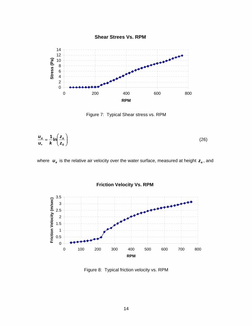
Figure 7: Typical Shear stress vs. RPM

⎟⎟⎠

⎞⎜⎜⎝

⎛=

∗ 0ln1

zz

kuu aa (26)

where is the relative air velocity over the water surface, measured at height , and au az

Friction Velocity Vs. RPM

0

0.5

1

1.5

2

2.5

3

3.5

0 100 200 300 400 500 600 700 800

RPM

Fric

tion

Velo

city

(m/s

ec)

Figure 8: Typical friction velocity vs. RPM

14

41.0=k is the Von Karman coefficient. The anemometer was placed at

above the tank bottom where the water surface height measured from the bottom of the

tank is

m425.0

H . The expression for is: az

Hza −= 425.0 (27)

Equation (27) enables the calculation of the roughness:

⎟⎟⎠

⎞⎜⎜⎝

⎛−⋅=

∗uukzz a

a exp0 (28)

The air velocity at a height of 10 m above the water surface is found by (28) and (26):

⎟⎟⎠

⎞⎜⎜⎝

⎛=

0

*10

10lnzk

uU (29)

Roughness Vs. U10 (m)

00.0020.0040.0060.0080.01

0.0120.0140.0160.0180.02

0 10 20 30 40 50 6

U10 (m/sec)

Rou

ghne

ss (m

)

0

Figure 9: Roughness length in meters vs. , the extrapolated air speed 10 meters

above the water surface. The calculated “unphysical” roughness length

range is 0-20 mm.

10U

15

The non-dimensional drag coefficient is obtained by dividing the shear stress by the

dynamic pressure at the reference air velocity obtained in (29). The drag coefficient

is:

10U

2

10210

10 ⎟⎟⎠

⎞⎜⎜⎝

⎛== ∗

Uu

UC

a

sD ρ

τ (30)

Drag Coefficient vs. U10

00.00050.001

0.00150.002

0.00250.003

0.00350.004

0.0045

0 10 20 30 40 50 6

U10 (m/sec)

C D10

0

Figure 10: Drag coefficient vs. the extrapolated wind speed at a height of 10 meters

above the water surface.

The results for the drag coefficient vs. shown in Figure 10 are consistent with

those of Donealn (2004) who used momentum budget showing a steep increase in the

drag coefficient up to a wind speed of 25-30 m/sec and then leveling and a decrease of

the drag coefficient for a wind speed higher than 30 m/sec. This steep increase and

leveling of the drag coefficient is also consistent with recent deductions from

dropwindsondes deployed in hurricanes Powell (2003), although the highest C

10U

D10 in

Donealn’s work is 2.5 10-3 while our is 4.0 10-3 for air speed of 25-30 m/sec.

16

Friction velocity Vs. U10

0

0.5

1

1.5

2

2.5

3

0 10 20 30 40 50 6

U10 (m/sec)

u * (m

/sec

)

0

Figure 11: Friction velocity vs. the extrapolated wind speed at a height of 10

meters above the water surface.

The data in Figures 10 and 12 will be used later on to normalize the enthalpy transfer

coefficient with U10.

6. Enthalpy Transfer Experiments

6.1 Introduction and experimental apparatus

A schematic drawing for the tank equipped and modified for the enthalpy transfer

experiment is shown in figure 12. Submerged heating elements are powered using a 20

Volt transformer. During the experiments, the paddle moves the air over the water, and

the air motion enhances the enthalpy transfer from the water into the lab ambient

environment. Humidity and temperature sensors were placed in the room and this

information was fed into a Program Logic Controller (PLC). A thermocouple measures

the bulk temperature of the water in the tank and this information is also fed into the

PLC. The PLC controls the on-off power input into the heating elements so the water

temperature is kept equal (within a margin of 0.2 C) to the lab ambient temperature. In

this way, heat transfer from the room into the tank through the tank walls is minimized.

17

The water level in the tank during all the enthalpy transfer experiments was 14 cm. This

water height, which was also used for the drag experiments, gave consistent results.

Each experiment was conducted using Poland SpringsTM water and the water was

always changed after each experiment. Each experiment was conducted over 24-48

hours. The surface tension of the water was measured before and after an experiment

and was found to be constant, having a value of 75-80 dyne/cm.

The water in the tank was connected by a pipe to an external cup so the water levels in the tank and the cup are equal. A needle attached to a micrometer is used to gauge the water level in the cup before and after the experiment, measuring the water loss during the experiment. The water level in the tank during the experiment was kept at

. If necessary, the experiment was briefly interrupted and a known amount of

water was added. Each experiment was done for a specific RPM. Air velocity vs. RPM was measured using an anemometer at a specified height above the water surface, as in the drag experiments.

cm114 ±

18

Figure 12: Wind wave tank equipped with heating elements The electric motor has an efficiency of less than 100% in converting electric power to

shaft power, thus the motor heats the surrounding motor case, thereby heating the

surrounding water. To solve this, a fan was installed in a duct to ventilate the motor.

6.2 Latent Enthalpy Transfer

The following formulation and analysis shows that for an experiment in which the water

and the ambient temperature are equal, the latent enthalpy transfer and the mass

transfer coefficients are equal.

The latent enthalpy transfer from the water is:

( )airVairsatwVwsataqwV LLAVCLm ,,,,, ρφρ −= (31)

where is the mass rate of evaporation, is the latent heat of evaporation at the

temperature of the water, is the latent heat of evaporation at the temperature of

the air, is the latent enthalpy transfer coefficient, is the air velocity,

m wVL ,

airVL ,

qC aV A is the water

surface area, φ is the relative humidity, and wsat ,ρ and airsat ,ρ are the saturation water

vapor density at the water and air temperature respectively.

Because the heating elements keep the water temperature equal to the air temperature,

and airVwV LL ,, = airsatwsat ,, ρρ = . Therefore, eq. (31) is reduced to give:

( )φρ −= 1,wsataq AVCm (32)

or

( )φρ −=

1,wsataq AV

mC (33)

19

The last expression for - the latent enthalpy transfer coefficient - is equivalent to the

mass transfer coefficient for these specific experimental conditions.

qC

Eq. (32) can also be written as ( φρ −= 1,wsataq AVCdtdm ) . Integrating:

( )∫∫ −==T

wsataqtot

m

dtAVCmdmtot

0,

0

1 φρ (34)

or ( )∫ −

= T

wsata

totq

dtAV

mC

0, 1 φρ

(35)

where is the total water mass evaporated in a specific experiment. In our

procedure, each experiment lasts

totm

min000,2000,1 −=n , and )(,, twsatwsat ρρ = and

)(tφφ = . The temperature and relative humidity (RH) are recorded once per minute.

Temperature Variations Over an Experiment

23.0023.2023.4023.6023.8024.0024.2024.4024.60

0 200 400 600 800 1000 1200 1400 160

Time (min)

Tem

pera

ture

(C)

Figure 13: Typical temperature variations over an enthalpy transfer experiment

The integral in (35) is written as a difference form and is performed numerically to give:

20

( )∑ Δ−= n

iwisata

totq

tAV

mC

1, 1 φρ

(36)

In fact, since the heating elements are activated by a temperature difference between

the ambient air and water, there are slight temperature differences between the water

and room temperature of about 0.3 C, on average. Therefore, equation (36) may be re-

written more accurately as:

∑ −Δ= n

iairsatiwisata

totq

tAV

mC

1,,, )( ρφρ

(37)

Relative Humidity variations

0.00

10.00

20.00

30.00

40.00

50.00

60.00

0 200 400 600 800 1000 1200 1400 1600

Time (min)

RH

(%)

Figure 14: Typical relative humidity variations over an enthalpy transfer experiment.

Since the tank walls are not perfectly circular, the cross sectional area of the tank was

measured around the height of the water surface using a known amount of water and

measuring its rise using the micrometer. The measured water surface area is

. Using this and 24769.0 mA = sec60=Δt (data recording interval by the

spreadsheet) Equation (37), it becomes:

21

∑ −= −

n

iairsatiwisata

totlatentq

V

mC

1,,,

2,

)(10495.3

ρφρ (38)

where is the total water mass evaporated in Kg during a specific experiment, is

the air speed in m s

totm aV-1, iφ is the relative humidity each minute. The saturation water

vapor pressure at the water surface and in the air as a function of temperature is

calculated using the semi-empirical Clausius-Clayperon equation (Ludlam, 1980):

⎥⎦

⎤⎢⎣

⎡−−

+=)86.35(

)16.273(27.178096.1exp100T

TPs (39)

where T is the temperature in K. The saturation vapor density is calculated using the

ideal gas equation:

TRPOH

ssat ⋅

=2

ρ (40)

where is the gas constant for water vapor. OHR2 KKg

JR OH ⋅= 5.461

2

Experiments were performed for 100, 120, 140…..480 RPM. The air velocity for each

RPM was measured using the anemometer, and the temperature of the water, ambient

air and relative humidity were recorded, enabling the calculation of

for each experiment. A summary of the latent enthalpy transfer

coefficient Vs. V

(∑ −n

iairsatiwisat1

,,, ρφρ )

0.285 is shown in figure 15. V0.285 is the air velocity at the height of the

anemometer placement, 0.285 m above the water surface.

Previously, the friction velocity vs. V0.285 has been found by experiment and therefore, it

is possible to calculate enthalpy transfer coefficient normalized with u* using:

*

285.0285.0,, * u

VCC qlatentq U⋅= (41)

22

Latent Enthalpy Transfer Coefficient Vs. Friction Velocity

0

0.01

0.02

0.03

0.04

0.05

0.06

0.07

0.08

0 0.5 1 1.5

Friction Velocity u* (m/sec)

Cq,

late

nt

2

Figure 15: Latent enthalpy transfer coefficient Cq, latent Vs. u* - the friction velocity. The

coefficient Cq, latent is normalized with u*.

The final step is to calculate the latent enthalpy transfer coefficient normalized with U10.

For this, it is possible to apply the data of friction velocity vs. the extrapolated wind

speed at a height of 10 meters above the water surface that was used to plot Figure 11

and the data of drag coefficient vs. the extrapolated U10 that was used to plot Figure 10.

For convenience, let’s denote the latent enthalpy transfer coefficient normalized with the

friction velocity as Cq* and the latent enthalpy transfer coefficient normalized with U10 as

Cq10. After some calculations it is possible to show that:

10*10 Dqq CCC ⋅= (42)

Or alternatively:

10

**10 U

uCC qq ⋅= (43)

23

Latent Enthalpy Transfer and Drag Coefficients vs. U10

0

0.001

0.002

0.003

0.004

0.005

0.006

0 10 20 30 40 50 6

U10 (m/sec)

Coe

ffici

ents

0

DragLatent Enthalpy

Figure 16: Extrapolation of latent enthalpy transfer and drag coefficients vs. U10.

Unfortunately, in the enthalpy transfer experiments it was impossible to reach high RPM

and air speed U10 higher than 32 m/sec. This was due to the absence of lid on the tank

that caused entrainment of air that added a load on power-limited electric motor.

7. Tank Limitations

A comparison between characteristics of a few experiments was made. Such a

comparison is important for identifying the limitations of the apparatus and to design

future experiments.

The false bottom is a valuable component of the facility. It can be used to vary the

distance from the paddle to the water surface without changing the amount of water in

the tank. Unfortunately, the possible height changes implemented by the false bottom

are no more than 20 cm owing to the height of the tank.

24

In further studies it might be useful to consider modifying the wind-wave tank by

increasing its height to about 3-5 meters. In such a tank, the false bottom position could

be changed by meters rather than centimeters. Also, a tall tank in which the paddle is

much higher than the water surface will prevent the water spray from reaching the

paddle blades.

At high RPM the water velocity Vw reached 1.5 - 1.7 m/sec. Owing to the parabolic

shape of the water surface (see appendix), the distance from the water surface to the

paddle near the outer wall is different from the distance near the inner wall. This

difference can reach 15 cm for .sec/7.1 mVw ≅ This introduces an error in calculating

, the distance from the water surface to the paddle and to the anemometer that

measures the air speed. The highly parabolic water surface for high RPM also alters the

moment of inertia of the water mass, and this introduces an error in the calculation of the

shear stress.

az

It was also observed that at a paddle RPM that corresponds to sec/3010 mU ≅ and

higher, water spray is generated, especially when the lid is on. It is estimated that the

centrifugal acceleration of the spray is on the order of so that its flight

time scale before impacting the tank walls is about 0.1 sec. This point may explain the

declining for and should be the subject of further investigation.

2sec/200100 m−

DC sec/2510 mU >

The enthalpy transfer experiments seem to provide useful and accurate information as

far as the latent enthalpy transfer is concerned. However, the tank air inflow and outflow

govern the sensible heat transfer, and this flow pattern in our experiment does not

resemble conditions over the ocean. In addition, at high RPM, mechanical dissipation in

the air above the water surface and on the tank walls might contribute to sensible heat

transfer into the water.

8. Conclusions

The scientific goal of this experimental study is to develop an experimental procedure for

estimating air-sea heat and momentum exchange at very high wind speeds, and to

present results for these fluxes in a relatively simple apparatus. While the limitations of

the circular tank make comparisons to nature problematic, we observe several

25

interesting features of the results that are consistent with other experiments. Our drag

experimental results are consistent with those of Donealn (2004) who used momentum

budget showing a steep increase in the drag coefficient up to a wind speed of 25-30

m/sec and then leveling and a decrease of the drag coefficient for a wind speed higher

than 30 m/sec. This steep increase and leveling of the drag coefficient is also consistent

with recent deductions from dropwindsondes deployed in hurricanes Powell (2003),

although the highest CD in Donealn’s work is 2.5 10-3 while our is 4.0 10-3 for air speed of

25-30 m/sec. All of this recent research seems to suggest that the well documented

increase in the surface drag coefficient with wind speed over the ocean does not

continue indefinitely but levels off at 10 m winds speeds of about marginal hurricane

force, and may even decrease at yet higher speeds. Consistent with the

abovementioned research, we observe such a decrease in the tank, but this decrease

may result from the centrifuging of spray before it can extract momentum from the

airflow. We hope to apply some of the estimation techniques described here in future

experiments using linear wind-wave flumes.

We also present quantitative estimates of the surface latent enthalpy exchange

coefficient at near hurricane wind speeds. The tank limitations did nit enable us to

conduct investigation into the sensible enthalpy exchange coefficient. The tank

limitations suggest caution in extrapolating these results to nature, they do suggest that

the enthalpy coefficient also increases with wind speed, but levels off near marginal

hurricane strength. The near equality of the enthalpy and momentum exchange

coefficients is consistent with what is required for quantitatively accurate forecasts of

hurricane intensity using numerical models (Emanuel, 1995). We hope to apply some of

the same experimental procedures developed here to deduce enthalpy fluxes in larger,

linear wind-wave flumes.

Acknowledgment: The authors wish to thank the MIT Edgerly Fund for providing the funding for the wind

wave tank construction and to Peter Morley and David Bono for their technical

assistance.

26

References: Alamaro, M.; “Wind Wave Tank for the Investigation of Momentum and Enthalpy

Transfer from the Ocean Surface at High Wind Speed,” Master thesis at the Department

of Earth, Atmospheric and Planetary Sciences, Massachusetts Institute of May, 2001.

See also: http://web.mit.edu/hurricanelab/ThesisWebsite.pdf

Bistre, M. and Emanuel, K.A., 1998: Dissipative heating and hurricane intensity.

Meteoric. Atoms. Physic. 65, 233-240.

Donelan, M.A. et al 2004: On the Limiting Aerodynamic Roughness of the Ocean in

Very Strong Winds. Forthcoming in Geophysical Research Letters.

Emanuel, K.A., 1986: An air-sea interaction theory for tropical cyclones. Part I.

J. Atmos. Sci., 42, 1062-1071.

Emanuel, K.A., 1988: The maximum intensity of hurricanes. J. Atmos. Sci.,

45, 1143-1155.

Emanuel, K.A., 1995: Sensitivity of tropical cyclones to surface exchange coefficients

and a revised steady-state model incorporating eye dynamics. J. Atmos. Sci., 52, 3969-

3976.

Fox, R.W, and McDonald, A.T. 1998: Introduction to Fluid Mechanics. John Wiley &

Sons, Inc., New York.

Geerneart, G. L., S. E. Larsen and F. Hansen, 1987: Measurements of the wind stress,

heat flux and turbulence intensity during storm conditions over the North Sea. J.

Geophys. Res., 92,13127-13139.

Ludlam, F.H., “Clouds and storms; the behavior and effect of water in the atmosphere,”

The Pennsylvania State University Press, 1980.

27

Ooyama, K., 1969: Numerical simulation of the life cycle of tropical cyclones. J. Atmos.

Sci., 26, 3-40.

Powell, M.D, et al 2003: Reduced Drag Coefficient for High Wind Speeds in Tropical

Cyclones. Nature, Vol. 422, 279-283.

Rosenthal, S. L., and M. S. Moss, 1971: Numerical experiments of relevance to Project

STORMFURY. NOAA Tech. Memo. ERL NHRL-95, Coral Gables, FL, 52 pp.

Appendix: Parabolic Shape Factors of the water surface

Due to the centrifugal acceleration, the water surface will not be horizontal. The water

surface becomes parabolic in r or )(rHH = . Therefore, the definition of , the height

above the water surface where air velocity is measured is compromised. The water

surface area and the water moment of inertia are also changed.

az

Consider rigid body rotation of the water mass. Equilibrium in the r direction at any point

in the water gives:

rr

Vdrdp 2

2Ω−=−= ρρ or r

drdzg

drdz

dzdp

drdp 2Ω−=−== ρρ (a1)

Integrating gives:

( ) (a2) 222

2)( inrr

grz −

Ω=Δ inrr ≥

Using D

w

RV

=Ω and substituting the values for and , equation (a1) provides the

height difference of the water surface between the outer water and inner walls for the

specific geometry of the tank:

0, rRD inr

20528.0 wVz =Δ (a3)

28

Where is in m swV -1

water

zΔr

drr +

ds

Figure a1: Parabolic surface of rotating rigid body water mass The differential surface area in the rotating system is:

rdsdA π2= or (a4) ∫=0

2)(r

rin

dsrrA π

Where:

drdrdzds

2

1 ⎟⎠⎞

⎜⎝⎛+= and (a1) becomes: r

gdrdz 2Ω

=

(a5)

Substituting and integrating:

⎥⎥⎥

⎦

⎤

⎢⎢⎢

⎣

⎡

⎟⎟⎠

⎞⎜⎜⎝

⎛ Ω+−⎟⎟

⎠

⎞⎜⎜⎝

⎛ Ω+⋅

Ω⋅=

23

22

423

22

4

4

211

32)( inr

gr

ggrA π (a6)

29

The parabolic area factor 0

0 )(ArAPFarea = is the ratio of the new water surface area to the

area of the surface without rotation and is obtained by substituting 0rr = and D

w

RV

=Ω

in equation (a6) so:

( )20

20

23

22

423

202

4

4

211

32

rr

rg

rg

g

PF

in

area −

⎥⎥⎥

⎦

⎤

⎢⎢⎢

⎣

⎡

⎟⎟⎠

⎞⎜⎜⎝

⎛ Ω+−⎟⎟

⎠

⎞⎜⎜⎝

⎛ Ω+⋅

Ω⋅

=π

π

(a7)

After substituting the apparatus dimensions and simplifying, the parabolic area factor become:

( ) ( )4

23

423

4 0407.0111578.01879.8

w

ww

area V

VVPF

⎥⎦

⎤⎢⎣

⎡+−+⋅

= (a8)

where is the water velocity in m swV -1. The increase in surface area due to rotation of

the water will be used to obtain the exchange rates per unit surface area. Similarly, an analysis has been made to define a parabolic torque correction factor for

the shear stress that propels the rotational water motion. The basic assumption is that

the shear stress over the water surface is not a function of the distance from the tank

center or that )(rss ττ ≠ . However, since the shear stress now is over a parabolic

surface, let’s denote the stress as pfτ (where the stand for parabolic factor). The

stress

pf

pfτ acts on a differential surface area dsr ⋅π2 and the differential torque

generated by the stress at a radial distance is: r

30

Increase of surface area due to rotation

1

1.1

1.2

1.3

1.4

1.5

1.6

0 0.5 1 1.5

water velocity (m/sec)

Para

bolic

are

a fa

ctor

2

Figure a2: The ratio of the surface area due to rotation to the surface area without

rotation as a function of the water velocity at the sonic Doppler location.

drdrdzrdsrrrdsdT pfpfpfpf

222 122)2( ⎟

⎠⎞

⎜⎝⎛+=== πτπτπτ (a9)

The solutions for pfτ becomes (Alamaro 2001):

( )torque

ss

D

wr

r

in

pf PFdrr

gRVr

rr

in

ττ

π

πτ =⋅

⎥⎥⎥⎥⎥⎥

⎦

⎤

⎢⎢⎢⎢⎢⎢

⎣

⎡

⎟⎟⎠

⎞⎜⎜⎝

⎛+

−=

∫ 224

42

330

12

32

0 (a10)

In equation (a10) the term in the bracket is a correction factor for the shear stress over a

parabolic water surface. Substituting the actual values for the apparatus dimensions

and we get: ,,,0 Din Rrr g

∫ +=out

in

r

rwtorque drrVrPF 242 504.0148.34 (a11)

31

The explicit expression for the solution of equation (a11) is a long and cumbersome

expression. Therefore, the integral in (a11) has been solved numerically for

. Curve fitting has been performed with a sixth degree polynomial to

obtain a working formula for the torque parabolic factor as a function of the water

velocity.

sec/20 mVw <<

The shear stress for the rotating water mass in the wind wave tank is obtained by

combining equations (13) and (a11) and by using the dimensions of the tank to obtain:

torque

w

pf PFt

VH∂∂

⋅⋅−=

1050τ (a12)

Where H is the water depth.

Torque Parabolic Factor Vs. Water Velocity

1

1.1

1.2

1.3

1.4

1.5

1.6

0 0.5 1 1.5

Water Velocity (m/sec)

Torq

ue P

arab

olic

Fac

tor

2

Figure a3: The correction factor to the propelling shear stress as a function of

water velocity at the radial location of the ADV.

32