EXPERIMENTAL EVALUATION OF GEOMEMBRANE / GEOTEXTILE ...
100
EXPERIMENTAL EVALUATION OF GEOMEMBRANE / GEOTEXTILE INTERFACE AS BASE ISOLATING SYSTEM A THESIS SUBMITTED TO THE GRADUATE SCHOOL OF NATURAL AND APPLIED SCIENCES OF MIDDLE EAST TECHNICAL UNIVERSITY BY AMIN TAHERI BONAB IN PARTIAL FULFILLMENT OF THE REQUIREMENTS FOR THE DEGREE OF MASTER OF SCIENCE IN CIVIL ENGINEERING APRIL 2016
Transcript of EXPERIMENTAL EVALUATION OF GEOMEMBRANE / GEOTEXTILE ...

EXPERIMENTAL EVALUATION OF GEOMEMBRANE / GEOTEXTILE
INTERFACE AS BASE ISOLATING SYSTEM
A THESIS SUBMITTED TO
THE GRADUATE SCHOOL OF NATURAL AND APPLIED SCIENCES
OF
MIDDLE EAST TECHNICAL UNIVERSITY
BY
AMIN TAHERI BONAB
IN PARTIAL FULFILLMENT OF THE REQUIREMENTS
FOR
THE DEGREE OF MASTER OF SCIENCE
IN
CIVIL ENGINEERING
APRIL 2016


Approval of the thesis:
EXPERIMENTAL EVALUATION OF GEOMEMBRANE / GEOTEXTILE
INTERFACE AS BASE ISOLATING SYSTEM
submitted by AMIN TAHERI BONAB in partial fulfillment of requirement for the
degree of Master of Science in Civil Engineering Department, Middle East
Technical University by:
Prof. Dr. Gülbin Dural Ünver
Dean, Graduate School of Natural and Applied Sciences
Prof. Dr. İsmail Özgür Yaman
Head of Department, Civil Engineering
Assoc. Prof. Dr. Zeynep Gülerce
Supervisor, Civil Engineering Dept., METU
Asst. Prof. Dr. Volkan Kalpakcı
Co-Supervisor, Civil Engineering Dept., HKU
Examining Committee Members:
Prof. Dr. Erdal Çokça
Civil Engineering Dept., METU
Assoc. Prof. Dr. Zeynep Gülerce
Civil Engineering Dept., METU
Asst. Prof. Dr. Volkan Kalpakcı
Civil Engineering Dept., HKU
Asst. Prof. Dr. Nabi Kartal Toker
Civil Engineering Dept., METU
Asst. Prof. Dr. Nejan Huvaj Sarıhan
Civil Engineering Dept., METU
Date:

iv
I hereby declare that all information in this document has been obtained
and presented in accordance with academic rules and ethical conduct. I also
declare that, as required by these rules and conduct, I have fully cited and
referenced all material and results that are not original to this work.
Name, Last Name: Amin, TAHERI BONAB
Signature:

v
ABSTRACT
EXPERIMENTAL EVALUATION OF GEOMEMBRANE / GEOTEXTILE
INTERFACE AS BASE ISOLATING SYSTEM
Taheri Bonab, Amin
M.S., Department of Civil Engineering
Supervisor: Assoc. Prof. Dr. Zeynep Gülerce
Co-Supervisor: Asst. Prof. Dr. Volkan Kalpakcı
April 2016, 82 pages
The objective of this study is to evaluate the effect of the composite liner
seismic isolation system on the seismic response of small-to-moderate height
structures. For this purpose, a building model with the natural frequency of 3.13 Hz
(representing 3-4 story structures) was tested with and without the addition of
composite liner system using the shaking table test set-up by employing harmonic
and modified/ scaled ground motions. Experiment results showed that the composite
liner seismic isolation system significantly reduced the floor accelerations, especially
in moderate-to-high ground shaking levels. The interaction between the natural
frequency of the model and the frequency of the loading is evaluated by integrating
the test results obtained here with previously conducted experiments on similar
models by Kalpakcı (2013). Analysis results displayed that the composite liner
system is most effective when these two frequencies are close to each other. Based
on the test results discussed here, a mean spectrum was derived to define the
behavior of the isolation system in frequency domain under ground motion
excitation.
Keywords: Seismic isolation, composite liner, geotextile, geomembrane, dynamic
tests, shaking table, building response.
vi
ÖZ
GEOMEMBRAN / GEOTEKSTİL ARAYÜZÜNÜN TEMEL IZOLASYONU
OLARAK KULLANILMASININ DENEYSEL OLARAK İNCELENMESİ
Taheri Bonab, Amin
Yüksek Lisans, İnşaat Mühendisliği Bölümü
Tez Yöneticisi: Doç. Dr. Zeynep Gülerce
Ortak Tez Yöneticisi: Yrd. Doç. Dr. Volkan Kalpakcı
Nisan 2016, 82 sayfa
Bu çalışmanın amacı kompozit sismik izolasyon sisteminin küçükten orta
yüksekliğe kadar olan yapıların sismik tepkileri üzerindeki etkisini
değerlendirmektir. Bu amaçla, 3-4 katlı yapıları temsil eden (doğal frekansı 3.13 Hz
olan) bir bina modeli, kompozit sistemin eklenmesiyle ve kompozit sistem olmadan
sarsma tablası üzerinde harmonik ve uyarlanmış yer hareketleri kullanarak test
edilmiştir. Deney sonuçları, kompozit sismik izolasyon sisteminin katlarda ölçülen
ivmeleri özellikle orta/yüksek yer hareketi seviyelerinde önemli ölçüde azalttığını
göstermiştir. Modelin doğal frekansı ile uygulanan hareketin frekansı arasındaki
etkileşimin incelenmesi için bu deney setinin sonuçları benzer modellerle daha önce
yapılmış deney sonuçları (Kalpakcı, 2013) ile birleştirilerek tekrar analiz edilmiştir.
Analiz sonuçları, bu iki frekansın birbirine yakın olduğu durumlarda kompozit
sistemin etkinliğinin arttığını işaret etmektedir. Test sonuçları kullanılarak, sismik
izolasyon sisteminin kuvvetli yer hareketleri altındaki davranışını tanımlayan
ortalama bir tepki spektrumu elde edilmiştir.
Anahtar Kelimeler: Sismik izolasyon, kompozit sistem, geotesktil, geomembran,
dinamik deneyler, sarsma tablası, tepki spektrumu.

vii
To my beloved family

viii
ACKNOWLEDGMENTS
The author wishes to express his sincere appreciation to his precious supervisor
Prof. Dr. Zeynep GÜLERCE
for her guidance, advice and encouragements throughout the research.
Asst. Prof. Dr. Volkan KALPAKCI
is sincerely acknowledged for his valuable support and contributions.
Finally, the author is grateful for the continuous support and encouragement
he has received from his family.

ix
TABLE OF CONTENTS
ABSTRACT ................................................................................................................. v
ÖZ ............................................................................................................................... vi
ACKNOWLEDGMENTS ........................................................................................ viii
TABLE OF CONTENTS ............................................................................................ ix
LIST OF FIGURES ..................................................................................................... x
LIST OF TABLES .................................................................................................... xvi
LIST OF SYMBOLS ............................................................................................... xvii
CHAPTERS
1. INTRODUCTION .................................................................................................... 1
2. PREVIOUS STUDIES ON THE SEISMIC RESPONSE OF COMPOSITE LINER
SYSTEM USED AS BASE ISOLATION ............................................................... 3
3. EXPERIMENTAL SETUP AND TESTING PROGRAM .................................... 19
2.1 Experimental Model Properties ........................................................................ 19
2.1.1 Free Vibration Test ........................................................................................ 24
2.2 Input Motions ................................................................................................... 25
4. EXPERIMENT RESULTS FOR 3-STORY BUILDING MODEL ...................... 29
4.1 Result of Tests with Harmonic Motions .......................................................... 32
4.2 Result of Tests with Scaled Ground Motions ................................................... 35
4.3 Verification of Fixed Base Model in CSI SAP2000 Software ......................... 39
5. COMPARISON OF THE CURRENT TEST RESULTS WITH PREVIOUSLY
PERFORMED EXPERIMENTS ........................................................................... 43
5.1 Comparison of Test Results for Harmonic Motions ........................................ 43
5.2 Comparison of Test Results for Ground Motions ............................................ 46
6. SUMMARY AND CONCLUSIONS ..................................................................... 55
REFERENCES ........................................................................................................... 57
APPENDICES
A. SAMPLE INPUT MOTION ................................................................................. 59
B. PROPERTIES OF SHAKING TABLE AND MEASUREMETN DEVICES ..... 61
C. GEOMEMBRANE AND GEOTEXTILE PROPERTIES .................................... 63
D. TIME HISTORIES OF INPUT GROUND MOTIONS ........................................ 65
x
LIST OF FIGURES
Figure 2.1 Conventional structures and base isolated structures (Naeim and Mayes,
2001) ............................................................................................................................. 3
Figure 2.2 (a) Elastomeric and (b) Sliding isolators .................................................... 4
Figure 2.3 Experiments using shaking table for geosynthetic interface in dry
condition with normal stress 1.2 psi (8.5 kPa) and for motions f=2,5,10 Hz (Yegian
and Lahlaf, 1992) ......................................................................................................... 6
Figure 2.4 Experiments using shaking table for geosynthetic interface in submerged
condition with normal stress 1.2 psi (8.5 kPa) and for motions f=2,5,10 Hz (Yegian
and Lahlaf, 1992) ......................................................................................................... 6
Figure 2.5 Accelerations transmitted through geosynthetic interfaces tested at 2 and 5
Hz (Yegian et al., 1999) ............................................................................................... 7
Figure 2.6 Single Story experimental model used in Yegian et al, 1999. .................... 8
Figure 2.7 Comparison of model responses with and without geosynthetic foundation
isolation. (Yegian et al, 1999) ...................................................................................... 9
Figure 2.8 Friction Coefficient vs. Normal Stress (Yegian and Kadakal, 2004) ....... 10
Figure 2.9 Maximum shaking table acceleration vs. transmitted acceleration during
harmonic excitation (Yegian and Kadakal, 2004) ...................................................... 10
Figure 2.10 Maximum shaking table acceleration vs. transmitted acceleration during
earthquake excitation (Yegian and Kadakal, 2004) ................................................... 10
Figure 2.11 Maximum acceleration of shaking table vs. model drift (Yegian and
Kadakal, 2004) ........................................................................................................... 11
Figure 2.12 (a) 2-story and (b) 4-story model used in Kalpakcı (2013) .................... 12
Figure 2.13 H/L vs. Acceleration for 2-Story Model (a) f= 1 Hz, (b) f= 2 Hz, (c) f= 3
Hz and ........................................................................................................................ 14
Figure 2.14 H/L vs. Acceleration for 4-Story Model (a) f= 1Hz, (b) f= 2 Hz, .......... 15
Figure 2.15 η vs. amax for (a) 2-story model (strike-slip), (b) 2-story model (reverse) ,
.................................................................................................................................... 16
Figure 0.1 Shaking table in soil laboratory of METU ................................................ 20
Figure 0.2 3-story model in fixed base mode ............................................................. 20
xi
Figure 0.3 Aluminum plates and the motion direction .............................................. 21
Figure 0.4 TDG Testbox 2010 data logger ................................................................ 21
Figure 0.5 Model in isolated base condition .............................................................. 22
Figure 0.6 UHMWPE geomembrane ......................................................................... 23
Figure 0.7 Small blocks of fiberglass covered with nonwoven heat-bonded geotextile
.................................................................................................................................... 23
Figure 0.8 Nonwoven heat-bonded geotextile ........................................................... 23
Figure 0.9 Acceleration time history of model under free vibration test ................... 24
Figure 0.10 Scaled response spectra for the recordings taken from (a) Landers, (b)
Chalfant Valley, (c) Loma Prieta, (d) Coalinga, (e) Northridge, and (f) San Fernando
Earthquakes (Each scaled to 0.1, 0.2 and 0.3g) ......................................................... 27
Figure 4.1 Time history recorded at top slab under f1a0.16 motion before filtration 29
Figure 4.2 Filters applied in SeismoSignal software ................................................. 30
Figure 4.3 Time history recorded at top story under f1a0.16 motion after filtration . 30
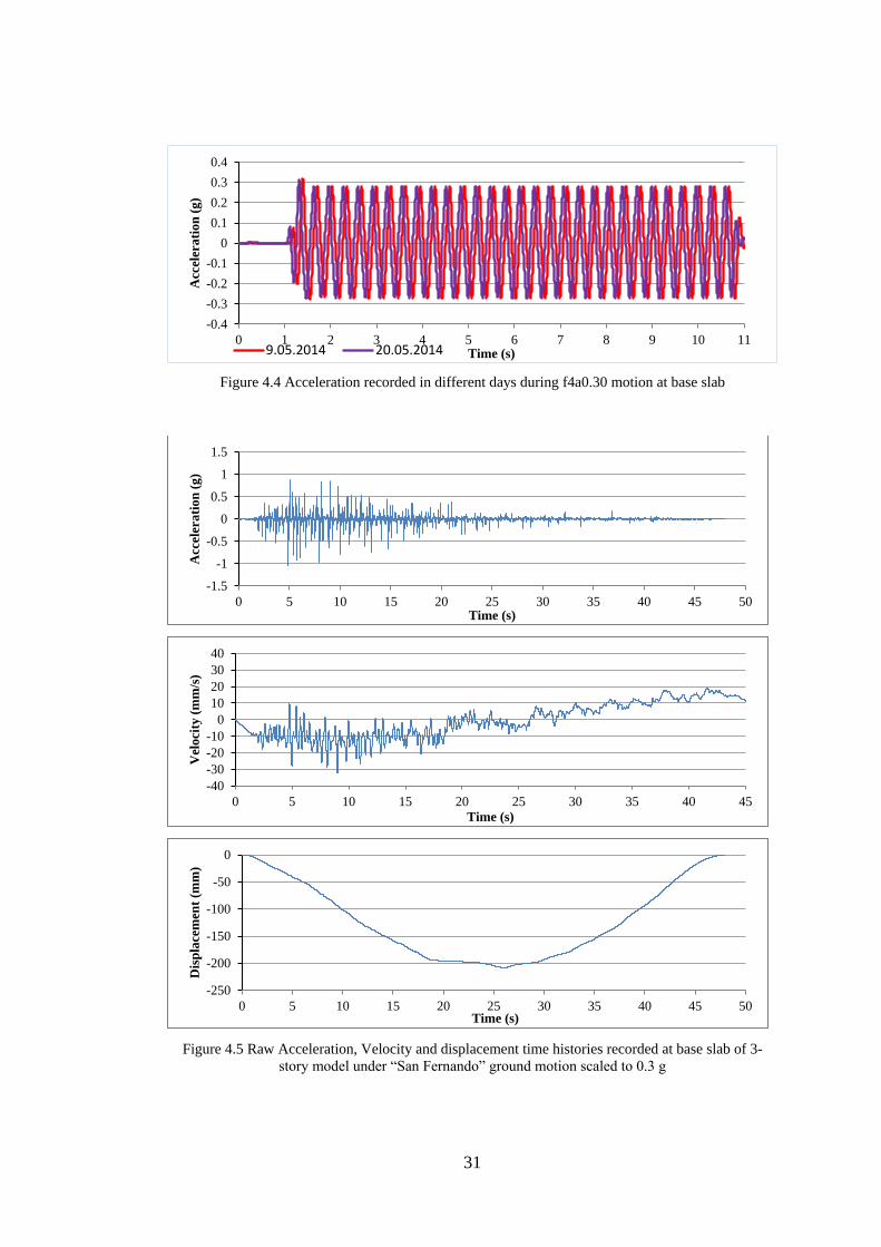
Figure 4.4 Acceleration recorded in different days during f4a0.30 motion at base slab
.................................................................................................................................... 31
Figure 4.5 Raw Acceleration, Velocity and displacement time histories recorded at
base slab of 3-story model under “San Fernando” ground motion scaled to 0.3 g .... 31
Figure 4.6 Filtered Acceleration, velocity and displacement time histories recorded at
base slab of 3-story model under “San Fernando” ground motion scaled to 0.3 g .... 32
Figure 4.7 Acceleration vs. H/L under f=1 Hz .......................................................... 33
Figure 4.8 Acceleration vs. H/L under f=2 Hz .......................................................... 33
Figure 4.9 Acceleration vs. H/L under f=3 Hz .......................................................... 33
Figure 4.10 Acceleration vs. H/L under f=4 Hz ........................................................ 33
Figure 4.11 Acceleration vs. H/L under Landers motions (f= 1Hz) .......................... 35
Figure 4.12 Acceleration vs. H/L under Coalinga motions (f= 1Hz) ........................ 35
Figure 4.13 Acceleration vs. H/L under Chalfant Valley motions (f= 2Hz) ............. 35
Figure 4.14 Acceleration vs. H/L under Northridge motions (f= 2Hz) ..................... 35
Figure 4.15 Acceleration vs. H/L under Loma Prieta motions (f= 4Hz) ................... 36
Figure 4.16 Acceleration vs. H/L under San Fernando motions (f= 4Hz) ................. 36
Figure 4.17 Mean Response Spectra for motions with f=1Hz scaled to 0.1g at top and
base of the 3-story model ........................................................................................... 37
xii
Figure 4.18 Mean Response Spectra for motions with f=2Hz scaled to 0.1g at top and
base of the 3-story model ........................................................................................... 37
Figure 4.19 Mean Response Spectra for motions with f=4Hz scaled to 0.1g at top and
base of the 3-story model ........................................................................................... 38
Figure 4.20 Mean Response Spectra for motions with f=1Hz scaled to 0.2g at top and
base of the 3-story model ........................................................................................... 38
Figure 4.21 Mean Response Spectra for motions with f=2Hz scaled to 0.2g at top and
base of the 3-story model ........................................................................................... 38
Figure 4.22 Mean Response Spectra for motions with f=4Hz scaled to 0.2g at top and
base of the 3-story model ........................................................................................... 38
Figure 4.23 Mean Response Spectra for motions with f=1Hz scaled to 0.3g at top and
base of the 3-story model ........................................................................................... 38
Figure 4.24 Mean Response Spectra for motions with f=2Hz scaled to 0.3g at top and
base of the 3-story model ........................................................................................... 38
Figure 4.25 Mean Response Spectra for motions with f=4Hz scaled to 0.3g at top and
base ............................................................................................................................. 39
Figure 4.26 SAP2000 Model ...................................................................................... 40
Figure 4.27 Acceleration vs. H/L under Landers motions in SAP2000 and
Experiments ................................................................................................................ 41
Figure 4.28 Acceleration vs. H/L under Chalfant Valley motions in SAP2000 and
Experiments ................................................................................................................ 41
Figure 4.29 Acceleration vs. H/L under Loma Prieta motions in SAP2000 and
Experiments ................................................................................................................ 41
Figure 4.30 Acceleration vs. H/L under Coalinga motions in SAP2000 and
Experiments ................................................................................................................ 41
Figure 4.31 Acceleration vs. H/L under Northridge motions in SAP2000 and
Experiments ................................................................................................................ 41
Figure 4.32 Acceleration vs. H/L under San Fernando motions in SAP2000 and
Experiments ................................................................................................................ 41
Figure 4.33 Comparison of the response spectra at the top and at the base gathered
from SAP2000 model and the experiments for the ground motion from Loma Prieta
earthquake scaled to amax=0.2g (LMP-0.2) ................................................................ 42

xiii
Figure 5.1 aIB/aFB vs. H/L for f1a0.08 motion ............................................................ 44
Figure 5.2 aIB/aFB vs. H/L for f1a0.30 motion ............................................................ 44
Figure 5.3 aIB/aFB vs. H/L for f3a0.08 motion ............................................................ 44
Figure 5.4 aIB/aFB vs. H/L for f1a0.30 motion ............................................................ 44
Figure 5.5 Mean of aIB/aFB vs freq. of model at top and base for f=1 Hz motions ..... 45
Figure 5.6 Mean of aIB/aFB vs freq. of model at top and base for f=2 Hz motions .... 45
Figure 5.7 Mean of aIB/aFB vs freq. of model at top and base for f=3 Hz motions .... 45
Figure 5.8 Mean of aIB/aFB vs freq. of model at top and base for f=4 Hz motions .... 45
Figure 5.9 aIB/aFB vs. H/L for LND_0.1 motion ......................................................... 47
Figure 5.10 aIB/aFB vs. H/L for LND_0.2 motion ....................................................... 47
Figure 5.11 aIB/aFB vs. H/L for LND_0.3 motion ....................................................... 47
Figure 5.12 aIB/aFB vs. H/L for LMP_0.1 motion ....................................................... 47
Figure 5.13 aIB/aFB vs. H/L for LMP_0.2 motion ....................................................... 47
Figure 5.14 aIB/aFB vs. H/L for LMP_0.3 motion ....................................................... 47
Figure 5.15 Normalized Response Spectra for 2-Story Model under Strike-Slip
Ground Motions ......................................................................................................... 48
Figure 5.16 Normalized Response Spectra for 2-Story Model under Reverse Ground
Motion ........................................................................................................................ 48
Figure 5.17 Normalized Response Spectra for 3-Story Model under Strike-Slip
Ground Motion ........................................................................................................... 48
Figure 5.18 Normalized Response Spectra for 3-Story Model under Reverse Ground
Motion ........................................................................................................................ 48
Figure 5.19 Normalized Response Spectra for 4-Story Model under Strike-Slip
Ground Motion ........................................................................................................... 48
Figure 5.20 Normalized Response Spectra for 4-Story Model under Reverse Ground
Motion ........................................................................................................................ 48
Figure 5.21 Mean of Normalized Response Spectra for 2-Story Model under Strike-
Slip and Reverse Ground Motions ............................................................................. 49
Figure 5.22 Mean of Normalized Response Spectra for 3-Story Model under Strike-
Slip and Reverse Ground Motions ............................................................................. 49
Figure 5.23 Mean of Normalized Response Spectra for 4-Story Model under Strike-
Slip and Reverse Ground Motions ............................................................................. 49
xiv
Figure 5.24 Mean of Normalized Response Spectra for All Models under Strike-Slip
and Reverse Ground Motions ..................................................................................... 50
Figure 5.25 Special Design Acceleration Spectra According to Turkish Earthquake
Code 2007 .................................................................................................................. 51
Figure 5.26 Fitted curve to Mean of Normalized Response Spectra for All Models in
FB Condition .............................................................................................................. 52
Figure 5.27 Fitted curve to Mean of Normalized Response Spectra for All Models in
IB Condition ............................................................................................................... 52
Figure 5.28 Fitted Curves for Mean of Normalized Response Spectra for FB and IB
conditions ................................................................................................................... 53
Figure D.1 Acceleration, velocity and displacement time histories for “Landers”
ground motion scaled to 0.1 g .................................................................................... 65
Figure D.2 Acceleration, velocity and displacement time histories for “Landers”
ground motion scaled to 0.2 g .................................................................................... 66
Figure D.3 Acceleration, velocity and displacement time histories for “Landers”
ground motion scaled to 0.3 g .................................................................................... 67
Figure D.4 Acceleration, velocity and displacement time histories for “Chalfant
Valley” ground motion scaled to 0.1 g ....................................................................... 68
Figure D.5 Acceleration, velocity and displacement time histories for “Chalfant
Valley” ground motion scaled to 0.2 g ....................................................................... 69
Figure D.6 Acceleration, velocity and displacement time histories for “Chalfant
Valley” ground motion scaled to 0.3 g ....................................................................... 70
Figure D.7 Acceleration, velocity and displacement time histories for “Loma Prieta”
ground motion scaled to 0.1 g .................................................................................... 71
Figure D.8 Acceleration, velocity and displacement time histories for “Loma Prieta”
ground motion scaled to 0.2 g .................................................................................... 72
Figure D.9 Acceleration, velocity and displacement time histories for “Loma Prieta”
ground motion scaled to 0.3 g .................................................................................... 73
Figure D.10 Acceleration, velocity and displacement time histories for “Coalinga”
ground motion scaled to 0.1 g .................................................................................... 74
Figure D.11 Acceleration, velocity and displacement time histories for “Coalinga”
ground motion scaled to 0.2 g .................................................................................... 75

xv
Figure D.12 Acceleration, velocity and displacement time histories for “Coalinga”
ground motion scaled to 0.3 g .................................................................................... 76
Figure D.13 Acceleration, velocity and displacement time histories for “Northridge”
ground motion scaled to 0.1 g .................................................................................... 77
Figure D.14 Acceleration, velocity and displacement time histories for “Northridge”
ground motion scaled to 0.2 g .................................................................................... 78
Figure D.15 Acceleration, velocity and displacement time histories for “Northridge”
ground motion scaled to 0.3 g .................................................................................... 79
Figure D.16 Acceleration, velocity and displacement time histories for “San
Fernando” ground motion scaled to 0.1 g .................................................................. 80
Figure D.17 Acceleration, velocity and displacement time histories for “San
Fernando” ground motion scaled to 0.2 g .................................................................. 81
Figure D.18 Acceleration, velocity and displacement time histories for “San
Fernando” ground motion scaled to 0.3 g .................................................................. 82
xvi
LIST OF TABLES
Table 2.1 Static friction angle (Yegian and Lahlaf, 1992) ........................................... 5
Table 2.2 Dynamic friction angle (Yegian and Lahlaf, 1992) ..................................... 5
Table 2.3 Interfaces and their friction coefficient used in Yegian and Kadakal, 2004.9
Table 2.4 Properties of input harmonic motions used in Kalpakcı (2013) ................ 13
Table 2.5 Properties of input modified ground motions used in Kalpakcı (2013) ..... 13
Table 0.1 Frequencies and amplitudes of selected harmonic motion combinations .. 25
Table 0.2 Summary of Input Ground Motions ........................................................... 26
Table B.1 Properties of shaking table used in METU soil laboratory ....................... 61
Table B.2 specification of data logger used in experiments ...................................... 61
Table B.3 Specification of measurement devices used in experiments ..................... 62
Table C.4 Material Properties of nonwoven heat-bonded Geotextile (Typar-3601) . 63
Table C.5 Physical and Mechanical Properties of UHMWPE Geomembrane (TIVAR
88-2) ........................................................................................................................... 63
Table C.6 Chemical Resistance Properties of UHMWPE Geomembrane (TIVAR 88-
2) ................................................................................................................................. 64
xvii
LIST OF SYMBOLS
Ab: Base area
D: Critical damping ratio
di= amplitude at ith cycle
FB: Fixed base condition
H: Height of story at which acceleration was measured
IB: Isolated base condition
L: Total height of model
Pm: base pressure of model
Wm: weight of model

xviii

1
CHAPTER 1
INTRODUCTION
Turkey and other earthquake-prone countries frequently experience moderate to large
magnitude earthquakes. These earthquakes mostly result in loss of lives and collapse
of most of the improperly built structures, especially in developing countries (e.g.
2010 Chile Earthquake). Isolating the building from the ground shaking is one of the
methods that has been proposed to avoid such collapses. Various types of seismic
isolators (e.g. elastomeric bearings, sliding bearings) have been designed for special
structures all around the world; however, the use of these seismic isolators have still
not become a standard practice in Turkey and in other developing countries mainly
due to their high initial costs and difficulties in their installation. In the last two
decades, many research efforts were focused on designing innovative seismic
isolators with lower costs and application ease. One of the recently developed
systems, known as the “composite liner system”, combines geotextiles and
geomembranes to be used as base isolators. Shaking table studies that test the
dynamic properties of composite liners with rigid blocks on top are available in the
literature and the details of these experiments are provided in Chapter 2. Similar
tests on composite liner system were also conducted on the shaking table test set-up
located in the Middle East Technical University Soil Mechanics Laboratory, using 2-
story and 4-story building models since the blocks in previous studies were rigid and
consequently had a higher natural frequency than typical buildings (Kalpakcı, 2013).
Chapter 2 also includes a detailed summary of the tests performed by Kalpakcı
(2013).
Kalpakcı (2013) noted that the frequency of the loading has a significant effect on
the efficiency of the composite liner system. Since the previous tests are limited with
only two models, 2-story and 4-story models with the scale of 1:12, the results could
not be fully utilized to analyze these effects in a systematic manner. One of the
objectives of this study is to complement the test results of Kalpakcı (2013) by
adding more data using a building model with a different natural frequency.
2
Therefore, a 3-story building model with the natural frequency of 3.13 Hz was
designed and tested by employing harmonic and modified ground motions in both
fixed base and isolated base conditions. The shaking table test set up, 3-story
building model, and the harmonic and modified ground motions used in the tests are
presented in Chapter 3. 69 experiments under different loading and base conditions
were performed and the acceleration time history of each floor was recorded during
these experiments. Tests results are given and thoroughly discussed in Chapter 4.
To understand the relation between the frequency of the harmonic load and the
natural frequency of the model, the test results gathered in this study was combined
with the results of 2-story and 4-story tests. The reduction in the floor accelerations
in the isolated base case when compared to the fixed base case is analyzed in
Chapter 5. Analysis results showed that the interaction between these two
frequencies has a significant effect on the efficiency of the composite liner system,
especially for harmonic loads. However, for modified and scaled ground motions,
this effect is not that substantial and the test results from all models can be combined
to analyze the reduction in the response. Combined results of tests with modified
ground motions are also presented in Chapter 5. The efficiency of the composite
liner system in reducing the spectral accelerations in a range of frequencies were
evaluated and a mean response spectra was derived to define the behavior of the
isolation system under ground motion excitation. Main conclusions of this study and
recommendations for future studies are provided in Chapter 6.
3
CHAPTER 2
PREVIOUS STUDIES ON THE SEISMIC RESPONSE OF COMPOSITE
LINER SYSTEM USED AS BASE ISOLATION
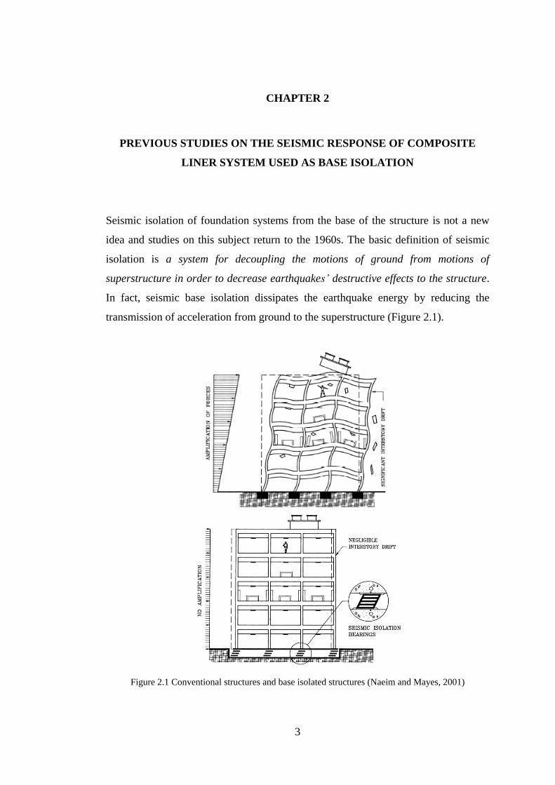
Seismic isolation of foundation systems from the base of the structure is not a new
idea and studies on this subject return to the 1960s. The basic definition of seismic
isolation is a system for decoupling the motions of ground from motions of
superstructure in order to decrease earthquakes’ destructive effects to the structure.
In fact, seismic base isolation dissipates the earthquake energy by reducing the
transmission of acceleration from ground to the superstructure (Figure 2.1).
Figure 2.1 Conventional structures and base isolated structures (Naeim and Mayes, 2001)

4
Various types of seismic isolation systems have been developed and used for this
purpose. Elastomeric and sliding isolators are the major types of seismic isolators,
which are used in developed countries (Figure 2.2). ‘Lead Rubber Bearing’ (LRB)
and ‘High Damping Rubber Bearing’ (HDRB) are mainly two types of elastomeric
isolators. ‘Sliding Support with Rubber-pad’ (SSR) and ‘Friction Pendulum System’
(FPS) are the types of sliding bearing systems.
(a)
(b)
Figure 2.2 (a) Elastomeric and (b) Sliding isolators
Since the application and implementation of seismic base isolation systems are costly
and requires expert and experienced staff to install, their application is limited to
public housing, schools, hospitals and structures with major importance. Therefore,
researchers have been attempting to find an easy-to-use, innovative and cost effective
approach to solve this problem. Using geomembrane and geotextile as a seismic
isolator is one of these new systems that researchers have been investigating for the
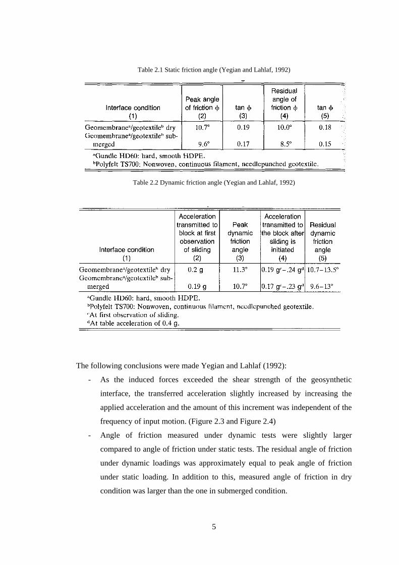
past few decades. In a study by Yegian and Lahlaf (1992), the static and dynamic
interface properties of geomembrane and geotextile was investigated. In their study,
static shear tests were performed in order to measure the static angle of friction
(Table 2.1). And also different shaking table tests with different frequencies and
normal stresses was performed on the selected geosynthetic combination in both dry
and submerged condition in order to measure the dynamic friction angle (Table 2.2).
5
Table 2.1 Static friction angle (Yegian and Lahlaf, 1992)
Table 2.2 Dynamic friction angle (Yegian and Lahlaf, 1992)
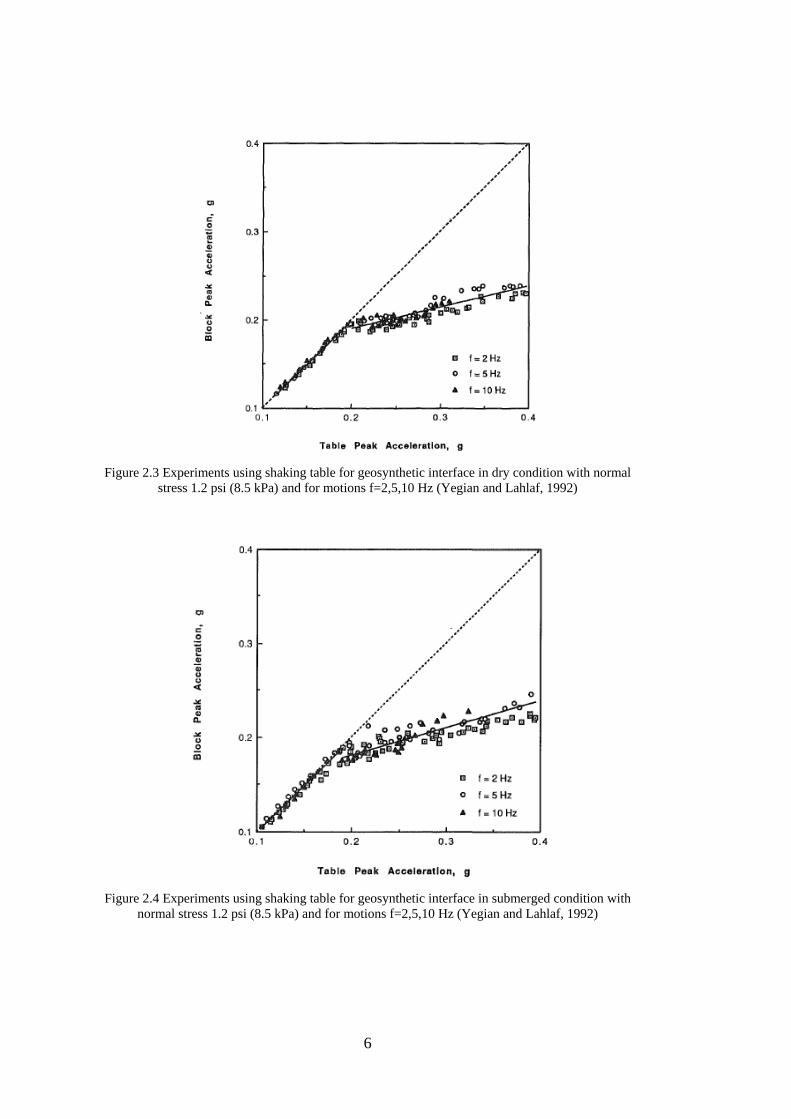
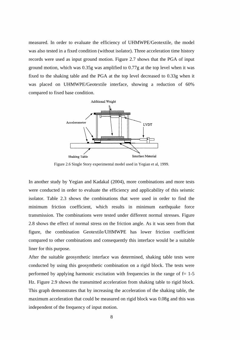
The following conclusions were made Yegian and Lahlaf (1992):
- As the induced forces exceeded the shear strength of the geosynthetic
interface, the transferred acceleration slightly increased by increasing the
applied acceleration and the amount of this increment was independent of the
frequency of input motion. (Figure 2.3 and Figure 2.4)
- Angle of friction measured under dynamic tests were slightly larger
compared to angle of friction under static tests. The residual angle of friction
under dynamic loadings was approximately equal to peak angle of friction
under static loading. In addition to this, measured angle of friction in dry
condition was larger than the one in submerged condition.
6
Figure 2.3 Experiments using shaking table for geosynthetic interface in dry condition with normal
stress 1.2 psi (8.5 kPa) and for motions f=2,5,10 Hz (Yegian and Lahlaf, 1992)
Figure 2.4 Experiments using shaking table for geosynthetic interface in submerged condition with
normal stress 1.2 psi (8.5 kPa) and for motions f=2,5,10 Hz (Yegian and Lahlaf, 1992)

7
In a study by Yegian et al. (1999), the use of geosynthetic materials as seismic
energy dissipation system was investigated. Geosynthetic or related materials that are
placed under foundations can absorb seismic energy, and hence transmit limited
shear forces and consequently smaller levels of excitation to an overlying structure.
Three following combinations of interfaces were chosen for shaking table tests:
Smooth HDPE/HDPE;
Smooth HDPE/Nonwoven spun-bonded Geotextile;
Polytetrafluoroethylene (PTFE)/PTFE.
In order to determine friction coefficients of tested interfaces, shaking table tests
were carried out and the interface with minimum friction coefficient was chosen,
since the minimum friction causes the maximum decrease in earthquake induced
forces. However, the interface’s friction coefficient had to be independent of the slip
rate. Results of shaking table tests under cyclic loading utilizing these three
combinations of different interfaces showed that the transmitted acceleration through
UHMWPE/Geotextile interface was lower than other combinations (Figure 2.5). The
‘Ultra High Molecular Weight Polyethylene’ (UHMWPE)/Geotextile interface which
has the lower friction coefficient (independent of slip rate), was chosen for the future
shaking table tests.
Figure 2.5 Accelerations transmitted through geosynthetic interfaces tested at 2 and 5 Hz (Yegian et
al., 1999)
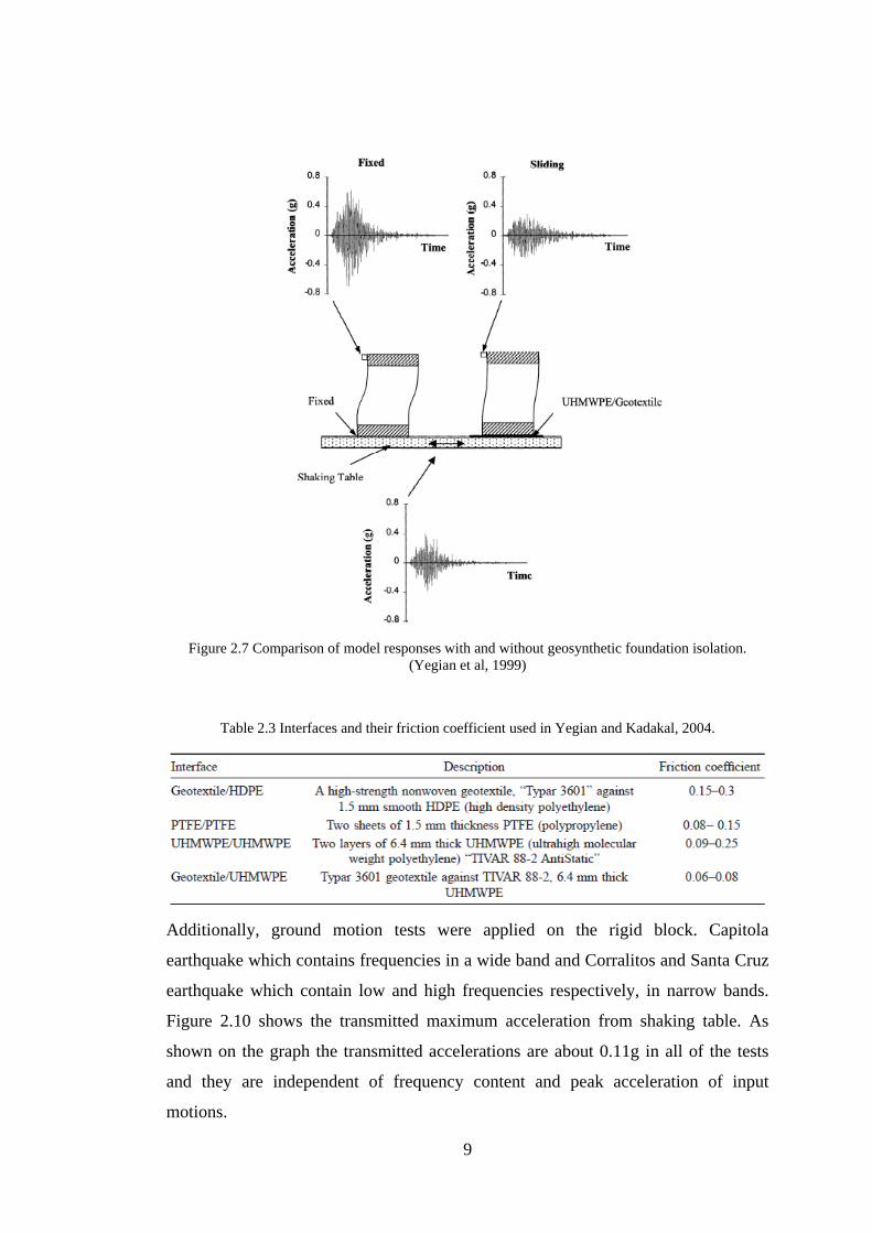
A single-story building model was tested on shaking table and UHMWPE/Geotextile
interface used as seismic isolator beneath the foundation of the model (Figure 2.6).
Acceleration at the top, base level and at the shaking table and the displacement were
8
measured. In order to evaluate the efficiency of UHMWPE/Geotextile, the model
was also tested in a fixed condition (without isolator). Three acceleration time history
records were used as input ground motion. Figure 2.7 shows that the PGA of input
ground motion, which was 0.35g was amplified to 0.77g at the top level when it was
fixed to the shaking table and the PGA at the top level decreased to 0.33g when it
was placed on UHMWPE/Geotextile interface, showing a reduction of 60%
compared to fixed base condition.
Figure 2.6 Single Story experimental model used in Yegian et al, 1999.
In another study by Yegian and Kadakal (2004), more combinations and more tests
were conducted in order to evaluate the efficiency and applicability of this seismic
isolator. Table 2.3 shows the combinations that were used in order to find the
minimum friction coefficient, which results in minimum earthquake force
transmission. The combinations were tested under different normal stresses. Figure
2.8 shows the effect of normal stress on the friction angle. As it was seen from that
figure, the combination Geotextile/UHMWPE has lower friction coefficient
compared to other combinations and consequently this interface would be a suitable
liner for this purpose.
After the suitable geosynthetic interface was determined, shaking table tests were
conducted by using this geosynthetic combination on a rigid block. The tests were
performed by applying harmonic excitation with frequencies in the range of f= 1-5
Hz. Figure 2.9 shows the transmitted acceleration from shaking table to rigid block.
This graph demonstrates that by increasing the acceleration of the shaking table, the
maximum acceleration that could be measured on rigid block was 0.08g and this was
independent of the frequency of input motion.
9
Figure 2.7 Comparison of model responses with and without geosynthetic foundation isolation.
(Yegian et al, 1999)
Table 2.3 Interfaces and their friction coefficient used in Yegian and Kadakal, 2004.
Additionally, ground motion tests were applied on the rigid block. Capitola
earthquake which contains frequencies in a wide band and Corralitos and Santa Cruz
earthquake which contain low and high frequencies respectively, in narrow bands.
Figure 2.10 shows the transmitted maximum acceleration from shaking table. As
shown on the graph the transmitted accelerations are about 0.11g in all of the tests
and they are independent of frequency content and peak acceleration of input
motions.

10
Figure 2.8 Friction Coefficient vs. Normal Stress (Yegian and Kadakal, 2004)
Figure 2.9 Maximum shaking table acceleration vs. transmitted acceleration during harmonic
excitation (Yegian and Kadakal, 2004)
Table Acceleration (g)
Figure 2.10 Maximum shaking table acceleration vs. transmitted acceleration during earthquake
excitation (Yegian and Kadakal, 2004)

11
Finally, all of ground motion tests were conducted on a one-story model in order to
investigate the effect of the geosynthetic combination on the drift. These tests were
conducted for fixed base and isolated base mode. Figure 2.11 shows that by
increasing the peak acceleration of input motion, model drift increases in fixed base
mode whereas in isolated base mode drift values are smaller than those in the fixed
base mode and remain constant.
Figure 2.11 Maximum acceleration of shaking table vs. model drift (Yegian and Kadakal, 2004)

12
In the study performed by Kalpakcı (2013), the efficiency of geosynthetic liner
similar to the one used in Yegian and Kadakal (2004) was investigated on two
different experimental models. 2-Story model with natural frequency of fn=4.35 Hz
and 4-Story model with the natural frequency of fn=2.33 Hz with the scale of 1:12
were prepared for this purpose (Figure 2.12). The models were tested in both fixed
base (FB) and isolated base (IB) conditions in order to evaluate the efficiency of the
geosynthetic liner, which was composed of UHMWPE (Ultra High Molecular
Weight Polyethylene) and nonwoven heat-bonded geotextile.
(a)
(b)
Figure 2.12 (a) 2-story and (b) 4-story model used in Kalpakcı (2013)
These models were tested under both harmonic motions and modified ground
motions. Harmonic motions were chosen with frequency of f=1 to 4 Hz in order to
cover the natural frequency of the experimental models. 4 different amplitudes were
combined with different frequencies of the harmonic motions in order to provide the
maximum acceleration of amax= 0.08, 0.16, 0.24 and 0.3 g. Table 2.4 shows the
details of harmonic motions used in Kalpakcı (2013).

13
Table 2.4 Properties of input harmonic motions used in Kalpakcı (2013)
Frequency (Hz) Displacement (mm)
1 20 40 60 75
2 5 10 15 18.75
3 2.22 4.44 6.66 8.33
4 1.25 2.5 3.75 4.69
Acceleration (g) 0.08 0.16 0.24 0.3
In addition to harmonic motions, these models also were tested under modified
ground motions. 6 earthquake recordings, three with strike-slip mechanism and three
with reverse mechanism were chosen in a way that predominant frequency of the
input motion is approximately equal to fn= 1, 2 and 4 Hz (Table 2.5). Amplitude of
these motions were scaled to amax= 0.1, 0.2 and 0.3g; therefore, each ground motion
is applied more than once with different scale factors.
Table 2.5 Properties of input modified ground motions used in Kalpakcı (2013)
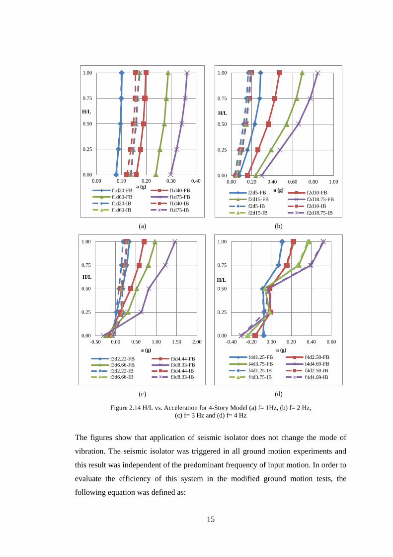
Figures 2.13 (a-d) and Figures 2.14 (a-d) demonstrate acceleration at each story vs.
H/L (H represents the height of story and L represents the total height of model) for
2-story and 4-story models respectively under harmonic motions. According to these
figures, triggering the system and the reduction of the acceleration depends on the
frequency of the input motion and independent of the amax of input motion. The
system is more efficient when the frequency of input motion is close to the natural
frequency of the experimental model.
Mechanism No Earthquake Date Station f (Hz)
Str
ike-
Sli
p 1 Landers 28.06.1992 Arcadia Av 1
2 Chalfant Valley 21.07.1986 Tinemaha Res 2
3 Loma Prieta 18.10.1989 Capitola 4
Rev
erse
1 Coalinga 02.05.1983 Park Field 1
2 Northridge 17.01.1994 Sylmar-County
Hospital 2
3 San Fernando 09.02.1971 Carbon Canyon
Dam 4

14
(a)
(b)
(c)
(d)
Figure 2.13 H/L vs. Acceleration for 2-Story Model (a) f= 1 Hz, (b) f= 2 Hz, (c) f= 3 Hz and
(d) f= 4 Hz
0.00
0.25
0.50
0.75
1.00
0.00 0.10 0.20 0.30 0.40
H/L
a (g)
f1d20-FB f1d40-FBf1d60-FB f1d75-FBf1d20-IB f1d40-IBf1d60-IB f1d75-IB
0.00
0.25
0.50
0.75
1.00
0.00 0.10 0.20 0.30 0.40
H/L
a (g)
f2d5-FB f2d10-FB
f2d15-FB f2d18.75-FB
f2d5-IB f2d10-IB
f2d15-IB f2d18.75-IB
0.00
0.25
0.50
0.75
1.00
0.00 0.20 0.40 0.60
H/L
a (g)
f3d2.22-FB f3d4.44-FB
f3d6.66-FB f3d8.33-FB
f3d2.22-IB f3d4.44-IB
f3d6.66-IB f3d8.33-IB
0.00
0.25
0.50
0.75
1.00
0.00 0.20 0.40 0.60 0.80
H/L
a (g)
f4d1.25-FB f4d2.50-FB
f4d3.75-FB f4d4.69-FB
f4d1.25-IB f4d2.50-IB
f4d3.75-IB f4d4.69-IB
15
(a)
(b)
(c)
(d)
Figure 2.14 H/L vs. Acceleration for 4-Story Model (a) f= 1Hz, (b) f= 2 Hz,
(c) f= 3 Hz and (d) f= 4 Hz
The figures show that application of seismic isolator does not change the mode of
vibration. The seismic isolator was triggered in all ground motion experiments and
this result was independent of the predominant frequency of input motion. In order to
evaluate the efficiency of this system in the modified ground motion tests, the
following equation was defined as:
0.00
0.25
0.50
0.75
1.00
0.00 0.10 0.20 0.30 0.40
H/L
a (g)f1d20-FB f1d40-FB
f1d60-FB f1d75-FB
f1d20-IB f1d40-IB
f1d60-IB f1d75-IB
0.00
0.25
0.50
0.75
1.00
0.00 0.20 0.40 0.60 0.80 1.00
H/L
a (g)f2d5-FB f2d10-FB
f2d15-FB f2d18.75-FB
f2d5-IB f2d10-IB
f2d15-IB f2d18.75-IB
0.00
0.25
0.50
0.75
1.00
-0.50 0.00 0.50 1.00 1.50 2.00
H/L
a (g)
f3d2.22-FB f3d4.44-FB
f3d6.66-FB f3d8.33-FB
f3d2.22-IB f3d4.44-IB
f3d6.66-IB f3d8.33-IB
0.00
0.25
0.50
0.75
1.00
-0.40 -0.20 0.00 0.20 0.40 0.60
H/L
a (g)
f4d1.25-FB f4d2.50-FB
f4d3.75-FB f4d4.69-FB
f4d1.25-IB f4d2.50-IB
f4d3.75-IB f4d4.69-IB

16
)(1F
I
a
a
(2.1)
In which,
Fa : The difference between acceleration of top and base floors, for FB condition;
Ia : The difference between acceleration of top and base floors, for IB condition.
(a)
(b)
(c)
(d)
Figure 2.15 η vs. amax for (a) 2-story model (strike-slip), (b) 2-story model (reverse) ,
(c) 4-story model (strike-slip), (d) 4-story model (reverse)
Figure 2.15 (a-d) shows the efficiency of the isolator for 2-story and 4-story models
respectively. As it can be seen in the graphs, the efficiency of the isolator system is
independent of predominant frequency of input motion however in experiments on
the 2-story model the system worked with higher efficiency as it coincides with
0
0.2
0.4
0.6
0.8
1
0.1 0.2 0.3
η
amax (g)
1Hz
2Hz
4Hz
0
0.2
0.4
0.6
0.8
1
0.1 0.2 0.3
η
amax(g)
1Hz2Hz4Hz
0
0.2
0.4
0.6
0.8
1
0.1 0.2 0.3
η
amax (g)
1Hz
2Hz
4Hz
0
0.2
0.4
0.6
0.8
1
0.1 0.2 0.3
η
amax (g)
1Hz
2Hz
4Hz

17
natural frequency of the model. Similar to the 2-story model, the seismic isolator is
also triggered for 4-story model and also was independent of predominant frequency
of the model. Another conclusion that could be drawn from the figures is that by
increasing the amax of input motion the efficiency of the system increases.

18

19
CHAPTER 3
EXPERIMENTAL SETUP AND TESTING PROGRAM
The shaking table test set-up used in this study is located in the Middle East
Technical University Soil Mechanics Laboratory. Design and production stages of
the shaking table along with its specifications were given in Kalpakcı (2013) and
Kalpakcı et al. (2014); therefore, only a brief summary will be provided in this
section. The servo-engine shaking table shown in Figure 3.1 is capable of performing
dynamic tests with harmonic and random motions along a single axis. However, the
applied motions are limited with the maximum frequency of 5 – 7 Hz (depending on
the payload, maximum 2 tons) and the maximum acceleration (amax) of 0.3g. Two
switches control the amplitude of shaking table and shut down the system completely
when the displacement of the table reaches to the limiting amplitude (±300 mm). The
external dimensions of the shaking table are 2m x 4m and its platform is 1m x 1.5m.
A laminar box of the same size in plan view can be attached to the table.
2.1 Experimental Model Properties
A 3-story model (composed of 3 stories and a base slab) that is consistent with the
experimental models of Kalpakcı (2013) was prepared with the scale of 1:12 for this
study (Figure 3.2). Slabs are made of fiberglass plates with dimensions of 35x50 cm
and with the thickness of 10 mm. These fiberglass plates were attached to 4
aluminum plates with the thickness of 1.5 mm and width of 3.5 cm at corners in a
way that the longer dimension the of aluminum plates are perpendicular to the
direction of motion to reduce the transverse and torsional movements during the tests
(as shown in Figure 3.3).
For recording the acceleration-time history at each story, four strain-gauge based
accelerometers with 1g measurement range were installed at the center of each floor.
Before each test, all of the accelerometers were re-calibrated and re-mounted on the
model since these accelerometers are highly sensitive to the voltage of the current in
the laboratory. In order to reduce the measurement errors; each test was performed

20
more than once on different days. The measured accelerations were collected by the
16-channel 24-bit resolution TDS TESTBOX2010 data acquisition system at the
sampling speed of 250 Hz (Figure 3.4).
Figure 0.1 Shaking table in soil laboratory of METU
Figure 0.2 3-story model in fixed base mode
htotal= 3×22 = 66 cm
Accelerometers

21
Figure 0.3 Aluminum plates and the motion direction
Figure 0.4 TDG Testbox 2010 data logger
In order to evaluate the efficiency of the composite liners for the purpose of seismic
base isolation, the model was tested on the shaking table both in ‘fixed base’ mode
(FB, Figure 3.2) and in ‘isolated base’ mode (IB, Figure 3.5). In FB experiments, the
model was fixed directly to the shaking table. During IB tests, a piece of UHMWPE
geomembrane (Figure 3.6) in 60x160 cm dimensions with the thickness of 6.4 mm
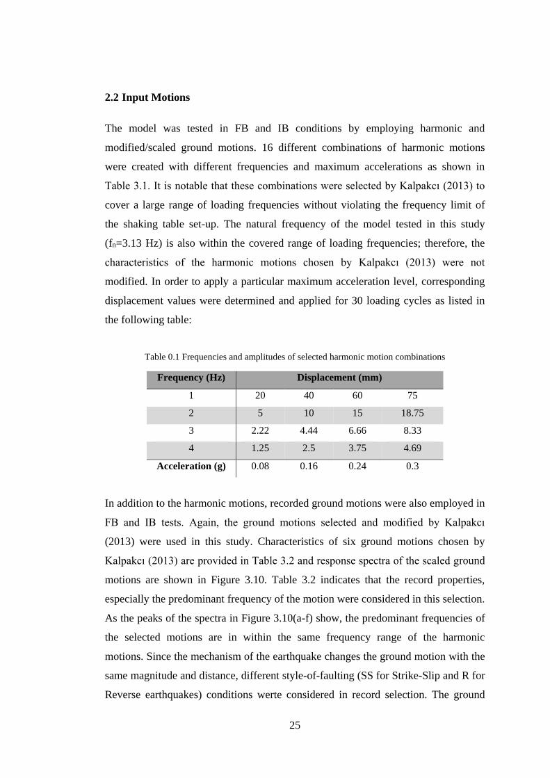
was fixed to the shaking table and 4 small blocks of fiberglass (Figure 3.7) covered
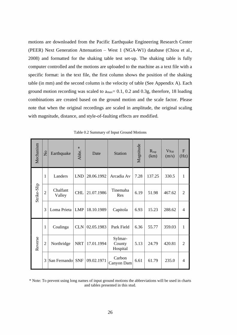
with nonwoven heat-bonded geotextile (Figure 3.8) were mounted to the base of the
model. Therefore, IB experiments utilize the friction between the geomembrane and
geotextile, not between the structure and the composite liner system. Specifications
of UHMWPE geomembrane and nonwoven heat-bonded geotextile are provided in
Appendix C.
Motion Direction
35
cm
50cm

22
Figure 0.5 Model in isolated base condition
The base pressure beneath the foundation of the model assumed to be as 40 kPa. In
order to simulate this pressure beneath the model in IB condition, the model was
weighed as 0.084 kN and the area of geotextile which will be in contact with
geomembrane was calculated as follows:
Pm= Wm / Ab (3.1)
Pm: base pressure of model
Wm: weight of model
Ab: base area
Ab= 0.084 ÷ 40 = 2100 mm2 (3.2)
The size of the four small fiberglass blocks used for attaching the geotextiles are
calculated as:
Ablock= 2100 ÷ 4 = 525 mm2 → 15 mm × 35 mm (3.3)
23
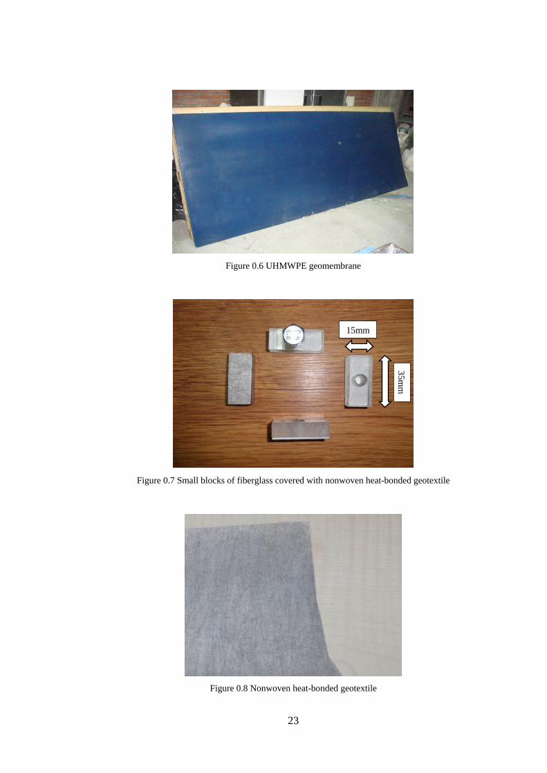
Figure 0.6 UHMWPE geomembrane
Figure 0.7 Small blocks of fiberglass covered with nonwoven heat-bonded geotextile
Figure 0.8 Nonwoven heat-bonded geotextile
35
mm
15mm

24
2.1.1 Free Vibration Test
As discussed in the previous chapter, the dimensions of the model were selected to
achieve a natural period that lies within 0.28-0.32 second range to complement the
previously conducted experiments. Free vibration tests were performed to determine
the natural period and the damping ratio of the models with different dimensions. In
these tests, the motion of the model was initiated by applying a small displacement to
the top of the model and the acceleration-time history of the top slab is recorded as
shown in Figure 3.9. Recorded time history is processed in SeismoSignal software to
estimate the natural frequency of the system. After a trial-and-error phase, the height
of each story was chosen as 22 cm and the natural frequency of the model is
measured as fn=3.13 Hz (Tn=0.32sec).
Figure 0.9 Acceleration time history of model under free vibration test
The damping ratio of the model is calculated as shown:
ln (di / di+n) = 2πnD
where, di is the amplitude at ith cycle, di+n is the amplitude at (i+n) th cycle, D is the
critical damping ratio. For this model, d3 = 0.0278 at t = 0.728 sec and d30 = 0.0043 at
t = 9.476 sec (n = 30-3 = 27); therefore, the damping ratio is:
ln (0.0278 / 0.0043) = 2π×27×D → D = 1.10 %
-0.04
-0.03
-0.02
-0.01
0
0.01
0.02
0.03
0.04
0 5 10 15 20
Acc
ele
rati
on
(g)
Time (sec)
25
2.2 Input Motions
The model was tested in FB and IB conditions by employing harmonic and
modified/scaled ground motions. 16 different combinations of harmonic motions
were created with different frequencies and maximum accelerations as shown in
Table 3.1. It is notable that these combinations were selected by Kalpakcı (2013) to
cover a large range of loading frequencies without violating the frequency limit of
the shaking table set-up. The natural frequency of the model tested in this study
(fn=3.13 Hz) is also within the covered range of loading frequencies; therefore, the
characteristics of the harmonic motions chosen by Kalpakcı (2013) were not
modified. In order to apply a particular maximum acceleration level, corresponding
displacement values were determined and applied for 30 loading cycles as listed in
the following table:
Table 0.1 Frequencies and amplitudes of selected harmonic motion combinations
Frequency (Hz) Displacement (mm)
1 20 40 60 75
2 5 10 15 18.75
3 2.22 4.44 6.66 8.33
4 1.25 2.5 3.75 4.69
Acceleration (g) 0.08 0.16 0.24 0.3
In addition to the harmonic motions, recorded ground motions were also employed in
FB and IB tests. Again, the ground motions selected and modified by Kalpakcı
(2013) were used in this study. Characteristics of six ground motions chosen by
Kalpakcı (2013) are provided in Table 3.2 and response spectra of the scaled ground
motions are shown in Figure 3.10. Table 3.2 indicates that the record properties,
especially the predominant frequency of the motion were considered in this selection.
As the peaks of the spectra in Figure 3.10(a-f) show, the predominant frequencies of
the selected motions are in within the same frequency range of the harmonic
motions. Since the mechanism of the earthquake changes the ground motion with the
same magnitude and distance, different style-of-faulting (SS for Strike-Slip and R for
Reverse earthquakes) conditions werte considered in record selection. The ground
26
motions are downloaded from the Pacific Earthquake Engineering Research Center
(PEER) Next Generation Attenuation – West 1 (NGA-W1) database (Chiou et al.,
2008) and formatted for the shaking table test set-up. The shaking table is fully
computer controlled and the motions are uploaded to the machine as a text file with a
specific format: in the text file, the first column shows the position of the shaking
table (in mm) and the second column is the velocity of table (See Appendix A). Each
ground motion recording was scaled to amax= 0.1, 0.2 and 0.3g, therefore, 18 loading
combinations are created based on the ground motion and the scale factor. Please
note that when the original recordings are scaled in amplitude, the original scaling
with magnitude, distance, and style-of-faulting effects are modified.
Table 0.2 Summary of Input Ground Motions
* Note: To prevent using long names of input ground motions the abbreviations will be used in charts
and tables presented in this stud.
Mec
han
ism
No
Earthquake
Abb
r. *
Date Station
Mag
nit
ude
Rrup
(km)
Vs30
(m/s)
F
(Hz)
Str
ike-
Sli
p
1 Landers LND 28.06.1992 Arcadia Av 7.28 137.25 330.5 1
2 Chalfant
Valley CHL 21.07.1986
Tinemaha
Res 6.19 51.98 467.62 2
3 Loma Prieta LMP 18.10.1989 Capitola 6.93 15.23 288.62 4
Rev
erse
1 Coalinga CLN 02.05.1983 Park Field 6.36 55.77 359.03 1
2 Northridge NRT 17.01.1994
Sylmar-
County
Hospital
5.13 24.79 420.81 2
3 San Fernando SNF 09.02.1971 Carbon
Canyon Dam 6.61 61.79 235.0 4

27
(a)
(b)
(c)
(d)
(e)
(f)
Figure 0.10 Scaled response spectra for the recordings taken from (a) Landers, (b) Chalfant Valley, (c)
Loma Prieta, (d) Coalinga, (e) Northridge, and (f) San Fernando Earthquakes (Each scaled to 0.1, 0.2
and 0.3g)
0
0.2
0.4
0.6
0.8
1
1.2
0 1 2 3 4
SP
EC
TR
AL
AC
CE
LE
RA
TIO
N (
G)
PERIOD (S)
Landers 0.1
Landers 0.2
Landers 0.3
0
0.2
0.4
0.6
0.8
1
1.2
0 1 2 3 4
SP
EC
TR
AL
AC
CE
LE
RA
TIO
N (
G)
PERIOD (S)
ChalfantValley 0.1
ChalfantValley 0.2
ChalfantValley 0.3
0
0.2
0.4
0.6
0.8
1
1.2
1.4
1.6
0 1 2 3 4
SP
EC
TR
AL
AC
CE
LE
RA
TIO
N (
G)
PERIOD (S)
LomaPrieta 0.1
LomaPrieta 0.2
LomaPrieta 0.3
0
0.2
0.4
0.6
0.8
1
1.2
1.4
0 1 2 3 4
SP
EC
TR
AL
AC
CE
LE
RA
TIO
N (
G)
PERIOD (S)
Coalinga 0.1
Coalinga 0.2
Coalinga 0.3
0
0.1
0.2
0.3
0.4
0.5
0.6
0.7
0.8
0.9
0 1 2 3 4
SP
EC
TR
AL
AC
CE
LE
RA
TIO
N (
G)
PERIOD (S)
Northridge 0.1
Northridge 0.2
Northridge 0.3
0
0.2
0.4
0.6
0.8
1
1.2
1.4
1.6
0 1 2 3 4
SP
EC
TR
AL
AC
CE
LE
RA
TIO
N (
G)
PERIOD (S)
SanFernando 0.1
SanFernando 0.2
SanFernando 0.3

28

29
CHAPTER 4
EXPERIMENT RESULTS FOR 3-STORY BUILDING MODEL
The 3-story building model described in Chapter 3 was tested by employing 16
different harmonic loading combinations and 18 different modified and scaled
ground motions in fixed base (FB) and isolated base (IB) conditions (68 experiments
in total). During these experiments, acceleration-time history at each floor is
recorded by accelerometers attached to the middle of the floors. Recorded raw time
histories include some measurement errors due to the vibration of the shaking table
set-up, minor time lag between the applied and recorded shaking, and the
fluctuations in the electrical current in the soil mechanics laboratory. The example
provided in Figure 4.1 clearly shows the measurement errors in the raw time history
recorded at the top story of the model during a harmonic motion experiment.
Figure 4.1 Time history recorded at top slab under f1a0.16 motion before filtration
To eliminate these errors, recorded raw accelerograms are filtered and baseline-
corrected using SeismoSignal and SeismoSpect software
(http://www.seismosoft.com). For this purpose, a-causal Butterforth filter with high-
pass and low-pass frequencies of 0.2 Hz and 6 Hz, respectively is used according to
criteria described by Douglas and Boore (2011) and Akkar et al. (2011) for modified
and scaled ground motions (Figure 4.2). For harmonic motions, the initial frequency
-0.3
-0.2
-0.1
0
0.1
0.2
0.3
0 5 10 15 20 25 30To
p-f
loor A
ccel
era
tio
n (
g)
Time (s)
30
range of the a-casual filter is chosen to be consistent with the predominant frequency
of input motion (generally within ±0.5 Hz) but modified for each recording to
produce a smooth and harmonic form of the recorded motion as shown in Figure 4.3.
Figure 4.2 Filters applied in SeismoSignal software
Figure 4.3 Time history recorded at top story under f1a0.16 motion after filtration
As it was mentioned before, in order to reduce the measurement errors, each test was
performed more than once on different days. Figure 4.4 shows the result of test under
harmonic motion with frequency of f=4 Hz and amax=0.30g performed on two
different days. It is clear from that there is not much difference between results of
these two experiments. Figures 4.5 and 4.6 shows the raw and filtered acceleration,
velocity and displacement time histories recorded at the base slab during San
Fernando ground motion scaled to 0.3g.
-0.3
-0.2
-0.1
0
0.1
0.2
0.3
0 5 10 15 20 25 30
To
p-f
loor A
ccel
era
tio
n (
g)
Time (s)
31
Figure 4.4 Acceleration recorded in different days during f4a0.30 motion at base slab
Figure 4.5 Raw Acceleration, Velocity and displacement time histories recorded at base slab of 3-
story model under “San Fernando” ground motion scaled to 0.3 g
-0.4
-0.3
-0.2
-0.1
0
0.1
0.2
0.3
0.4
0 1 2 3 4 5 6 7 8 9 10 11
Acc
eler
ati
on
(g)
Time (s)9.05.2014 20.05.2014
-1.5
-1
-0.5
0
0.5
1
1.5
0 5 10 15 20 25 30 35 40 45 50
Acc
eler
ati
on
(g)
Time (s)
-40
-30
-20
-10
0
10
20
30
40
0 5 10 15 20 25 30 35 40 45
Vel
ocit
y (
mm
/s)
Time (s)
-250
-200
-150
-100
-50
0
0 5 10 15 20 25 30 35 40 45 50
Dis
pla
cem
ent
(mm
)
Time (s)

32
Figure 4.6 Filtered Acceleration, velocity and displacement time histories recorded at base slab of 3-
story model under “San Fernando” ground motion scaled to 0.3 g
4.1 Result of Tests with Harmonic Motions
The test results of the experiments with harmonic loading combinations are shown in
Figures 4.7 to 4.10 for harmonic motions with 1 Hz, 2 Hz, 3 Hz, and 4 Hz
frequencies, respectively. Horizontal axis of Figures 4.7 to 4.10 shows the absolute
maximum value of the measured accelerations at each floor. The vertical axis of
these figures shows the H/L, which is defined as ratio of height of each floor to the
total height of the model (0 at the base and 1 at the top). Each motion is denoted by
fXaYY where X stands for the frequency of input motion and YY shows the
-0.4
-0.3
-0.2
-0.1
0
0.1
0.2
0.3
0.4
0 5 10 15 20 25 30 35 40 45 50
Acc
eler
ati
on
(g)
Time (s)
-20
-15
-10
-5
0
5
10
15
20
0 5 10 15 20 25 30 35 40 45
Vel
ocit
y (
mm
/s)
Time (s)
-3
-2
-1
0
1
2
3
0 5 10 15 20 25 30 35 40 45 50
Dis
pla
cem
ent
(mm
)
Time (s)

33
maximum acceleration of that particular motion. For instance, ‘f1a0.24’ is the motion
with the frequency of 1 Hz and the acceleration of 0.24g.
Figure 4.7 Acceleration vs. H/L under f=1 Hz
Figure 4.8 Acceleration vs. H/L under f=2 Hz
Figure 4.9 Acceleration vs. H/L under f=3 Hz
Figure 4.10 Acceleration vs. H/L under f=4 Hz
0.00
0.33
0.67
1.00
0 0.1 0.2 0.3 0.4
H/L
Acceleration (g)
FB-f1a0.08 FB-f1a0.16FB-f1a0.24 FB-f1a0.30IB-f1a0.08 IB-f1a0.16IB-f1a0.24 IB-f1a0.30
0.00
0.33
0.67
1.00
0 0.1 0.2 0.3 0.4 0.5H
/LAcceleration (g)
FB-f2a0.08 FB-f2a0.16FB-f2a0.24 FB-f2a0.30IB-f2a0.08 IB-f2a0.16IB-f2a0.24 IB-f2a0.30
0.00
0.33
0.67
1.00
0 0.5 1 1.5 2
H/L
Acceleration (g)
FB-f3a0.08 FB-f3a0.16
FB-f3a0.24 FB-f3a0.30
IB-f3a0.08 IB-f3a0.16
IB-f3a0.24 IB-f3a0.30
0.00
0.33
0.67
1.00
0 0.5 1 1.5
H/L
Acceleration (g)
FB-f4a0.08 FB-f4a0.16
FB-f4a0.24 FB-f4a0.30
IB-f4a0.08 IB-f4a0.16
IB-f4a0.24 IB-f4a0.30

34
Figures 4.7 – 4.10 show that:
When the input acceleration levels are small (e.g. blue and red curves in Figures
4.7, 4.8, and 4.10), the accelerations measured in FB and IB conditions are
approximately the same. Insignificant reduction in the accelerations in each floor
indicates that the base isolation system is not utilized (or triggered) for small
acceleration levels (for motions with amax = 0.08 and 0.16g).
If the input acceleration is higher than 0.16g, the accelerations measured for IB
cases at the top floor are significantly smaller than the accelerations measured at
the top floor for FB cases, showing that the base isolation system effectively
reduced the ground shaking levels.
When the frequency of the input motion is close to the natural frequency of the
system, the amplification of the response (the floor accelerations) is very large,
(measured top floor accelerations for FB case are close to or larger than 1g in
Figure 4.8). For this case, the base isolation system reduces the measured
accelerations even for small shaking levels.
The maximum accelerations are measured at the top floor in each test, except for
f=4 Hz FB tests (green and purple lines in Figure 4.10). It is notable that the mode
of the building model shifts to higher vibrational periods for these tests with large
base accelerations.
Amount of decrease in the base acceleration due to the base isolator is highly
dependent on the frequency of the input motion. As the input motion frequency
“f” gets closer to the natural frequency “fn” of the model (as increases from 1 Hz
to 4 Hz for this model), the reduction in the accelerations for IB condition relative
to FB condition is higher.
The composite liner system is most effective for motions with frequencies close to
the natural frequency of the model namely, f = 2 Hz and f = 3 Hz motions
recalling that the natural frequency of the model was fn = 3.13 Hz.
Test results for 4-story building model are consistent with the findings of
Kalpakcı (2013) for 2-story and 4-story building models. Comparison of the
results presented here and the tests results from Kalpakcı (2013) is provided in
Chapter 5.
35
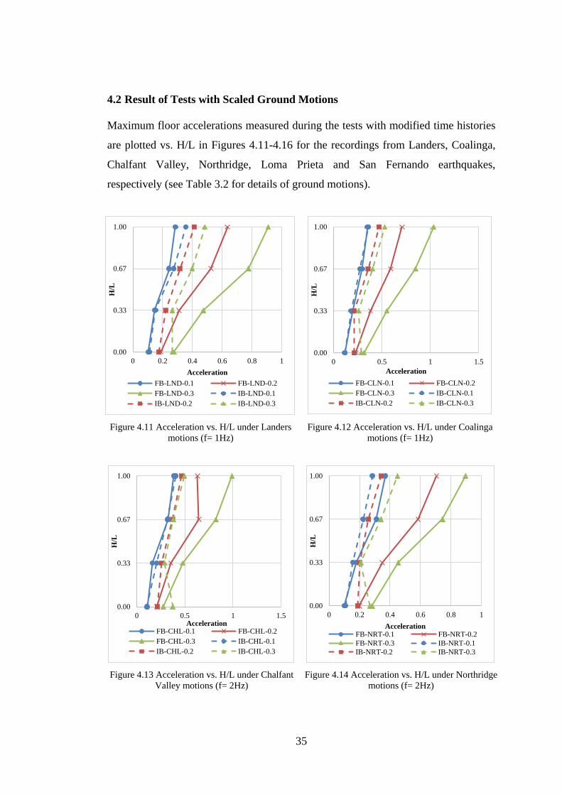
4.2 Result of Tests with Scaled Ground Motions
Maximum floor accelerations measured during the tests with modified time histories
are plotted vs. H/L in Figures 4.11-4.16 for the recordings from Landers, Coalinga,
Chalfant Valley, Northridge, Loma Prieta and San Fernando earthquakes,
respectively (see Table 3.2 for details of ground motions).
Figure 4.11 Acceleration vs. H/L under Landers
motions (f= 1Hz)
Figure 4.12 Acceleration vs. H/L under Coalinga
motions (f= 1Hz)
Figure 4.13 Acceleration vs. H/L under Chalfant
Valley motions (f= 2Hz)
Figure 4.14 Acceleration vs. H/L under Northridge
motions (f= 2Hz)
0.00
0.33
0.67
1.00
0 0.2 0.4 0.6 0.8 1
H/L
Acceleration
FB-LND-0.1 FB-LND-0.2
FB-LND-0.3 IB-LND-0.1
IB-LND-0.2 IB-LND-0.3
0.00
0.33
0.67
1.00
0 0.5 1 1.5
H/L
Acceleration
FB-CLN-0.1 FB-CLN-0.2
FB-CLN-0.3 IB-CLN-0.1
IB-CLN-0.2 IB-CLN-0.3
0.00
0.33
0.67
1.00
0 0.5 1 1.5
H/L
AccelerationFB-CHL-0.1 FB-CHL-0.2
FB-CHL-0.3 IB-CHL-0.1
IB-CHL-0.2 IB-CHL-0.3
0.00
0.33
0.67
1.00
0 0.2 0.4 0.6 0.8 1
H/L
AccelerationFB-NRT-0.1 FB-NRT-0.2
FB-NRT-0.3 IB-NRT-0.1
IB-NRT-0.2 IB-NRT-0.3

36
Figure 4.15 Acceleration vs. H/L under Loma Prieta
motions (f= 4Hz)
Figure 4.16 Acceleration vs. H/L under San
Fernando motions (f= 4Hz)
According to Figures 4.11-4.16:
Results of the tests with scaled ground motions are not significantly different
from the results of the tests with harmonic motions. Again, the floor
accelerations measured in FB and IB conditions for small shaking levels
(amax=0.1g) are close to each other, indicating that the base isolation system is
not triggered (solid and broken blue lines in Figures 4.11-4.16).
The composite liner system effectively reduces the floor accelerations for the
tests with amax=0.2g and amax=0.3g.
As the predominant frequency of the input motion increases from f=1 Hz to 4 Hz
the efficiency of the seismic isolator increases. When the predominant frequency
of the input motions is close to the natural frequency of the experimental model
(motions with predominant frequency of f= 4 Hz shown in Figures 4.15 and
4.16) the isolator system works well even for small acceleration levels and the
floor accelerations in IB case are significantly smaller than the floor
accelerations in FB conditions.
The change in vibrational period (mode) observed in harmonic tests with f=4 Hz
in FB conditions (Figure 4.10) is not observed in the tests with input motions
with the same predominant frequency (Figures 4.15 and 4.16).
0.00
0.33
0.67
1.00
0 0.5 1 1.5 2
H/L
Acceleration
FB-LMP-0.1 FB-LMP-0.2
FB-LMP-0.3 IB-LMP-0.1
IB-LMP-0.2 IB-LMP-0.3
0.00
0.33
0.67
1.00
0 0.5 1 1.5
H/L
Acceleration
FB-SNF-0.1 FB-SNF-0.2
FB-SNF-0.3 IB-SNF-0.1
IB-SNF-0.2 IB-SNF-0.3

37
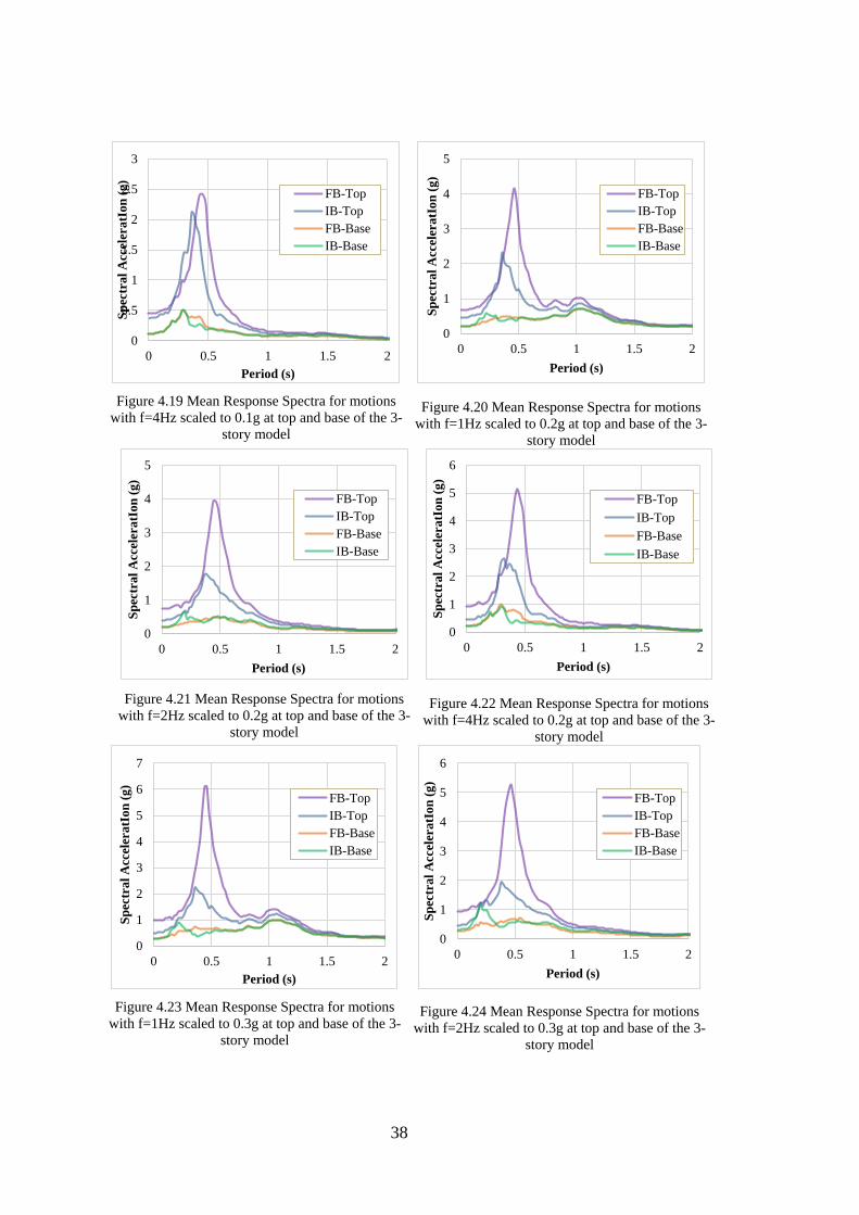
Mean response spectra measured at the top and the base floors in FB and IB cases are
presented in Figures 4.17 through 4.25. In these figures, the mean spectra are
calculated for the input motions scaled to the same maximum acceleration level and
with the same predominant frequency. For example, Figure 4.17 shows the mean
spectra of the time histories from Landers and Coalinga earthquakes (with f=1 Hz)
scaled to amax=0.1g that are recorded at the base and at the top floors in FB and IB
cases. Green and orange lines in each figure show that the response spectra recorded
at the base floor in IB and FB cases are similar to each other, especially in the long
period range. Minor differences are observed in the spectral accelerations for periods
close to the natural period of the system.
When the top and base spectra are compared, a very significant amplification in the
spectral acceleration values for 0.2-0.5 second periods (f=2-5 Hz) are observed in
each test (purple lines in Figures 4.17-4.25). This substantial increase in the response
can be explained by the effect of structural response of the building model on the
frequency content of the recorded ground motions. Test results show that the base
isolation system has a significant effect on this amplification. Contribution of the
base isolation system is not visible in Figures 4.17, 4.18 and 4.19 since the ground
shaking levels in these tests are small and the base isolation system is not triggered.
However, the base isolation system clearly reduces the amplification in 2-5 Hz
spectral accelerations in the tests with amax=0.2g and amax=0.3g (blue lines in Figures
4.20-4.25).
Figure 4.17 Mean Response Spectra for motions
with f=1Hz scaled to 0.1g at top and base of the 3-
story model
Figure 4.18 Mean Response Spectra for motions
with f=2Hz scaled to 0.1g at top and base of the 3-
story model
0
0.5
1
1.5
2
2.5
0 0.25 0.5 0.75 1 1.25 1.5 1.75 2
Sp
ectr
al
Acc
eler
atI
on
(g)
Period (s)
FB-Top
IB-Top
FB-Base
IB-Base
0
0.5
1
1.5
2
2.5
0 0.5 1 1.5 2
Sp
ectr
al
Acc
eler
atı
on
(g)
Period (s)
FB-Top
IB-Top
FB-Base
IB-Base
38
Figure 4.19 Mean Response Spectra for motions
with f=4Hz scaled to 0.1g at top and base of the 3-
story model
Figure 4.20 Mean Response Spectra for motions
with f=1Hz scaled to 0.2g at top and base of the 3-
story model
Figure 4.21 Mean Response Spectra for motions
with f=2Hz scaled to 0.2g at top and base of the 3-
story model
Figure 4.22 Mean Response Spectra for motions
with f=4Hz scaled to 0.2g at top and base of the 3-
story model
Figure 4.23 Mean Response Spectra for motions
with f=1Hz scaled to 0.3g at top and base of the 3-
story model
Figure 4.24 Mean Response Spectra for motions
with f=2Hz scaled to 0.3g at top and base of the 3-
story model
0
0.5
1
1.5
2
2.5
3
0 0.5 1 1.5 2
Sp
ectr
al
Acc
eler
atI
on
(g)
Period (s)
FB-Top
IB-Top
FB-Base
IB-Base
0
1
2
3
4
5
0 0.5 1 1.5 2
Sp
ectr
al
Acc
eler
atI
on
(g)
Period (s)
FB-Top
IB-Top
FB-Base
IB-Base
0
1
2
3
4
5
0 0.5 1 1.5 2
Sp
ectr
al
Acc
eler
atI
on
(g)
Period (s)
FB-Top
IB-Top
FB-Base
IB-Base
0
1
2
3
4
5
6
0 0.5 1 1.5 2
Sp
ectr
al
Acc
eler
atI
on
(g)
Period (s)
FB-Top
IB-Top
FB-Base
IB-Base
0
1
2
3
4
5
6
7
0 0.5 1 1.5 2
Sp
ectr
al
Acc
eler
atI
on
(g)
Period (s)
FB-Top
IB-Top
FB-Base
IB-Base
0
1
2
3
4
5
6
0 0.5 1 1.5 2
Sp
ectr
al
Acc
eler
atI
on
(g
)
Period (s)
FB-Top
IB-Top
FB-Base
IB-Base

39
Figure 4.25 Mean Response Spectra for motions
with f=4Hz scaled to 0.3g at top and base
4.3 Verification of Fixed Base Model in CSI SAP2000 Software
The building model used in these experiments was prepared using the scale of 1:12.
Same 4-story building model is also created in CSI SAP2000 software
(https://www.csiamerica.com/) but the scale is modified as shown in Figure 4.25. For
the SAP2000 model, the floor dimensions are taken as 4.2×6.0 m and the story height
is selected as 2.70 m. Slab thickness is defined as 15 cm and columns dimension are
determined in way that the natural frequency of the SAP2000 model would be
identical to the natural frequency of the building model (fn= 3.13 Hz). By assigning
47×70 cm dimensions to columns, the desired natural frequency is obtained in
SAP2000. Please note that only the fixed base condition is modelled, since the
seismic isolator system used in this study cannot be defined in SAP2000.
The response of the SAP2000 model is analyzed using the same set of scaled ground
motion recording used in the experiments. Acceleration-time history at each floor is
calculated using SAP2000 software and compared with the maximum floor
accelerations measured during the experiments as shown in Figures 4.26 – 4.31. In
these figures, the solid lines show the values calculated in SAP2000 whereas the
broken lines represent the measured values in experiments. According to Figures
4.26-4.31, calculated accelerations in SAP2000 software and the measured
accelerations during the experiments at base are the same. However, most of the
calculated and measured accelerations are different for the top floor: the measured
accelerations are greater than the calculated ones almost for all ground motions.
0
2
4
6
8
10
0 0.5 1 1.5 2S
pec
tra
l A
ccel
eratI
on
(g)
Period (s)
FB-Top
IB-Top
FB-Base
IB-Base
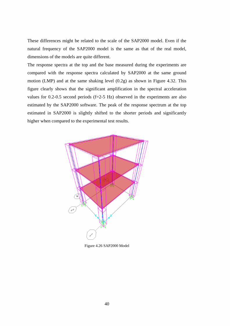
40
These differences might be related to the scale of the SAP2000 model. Even if the
natural frequency of the SAP2000 model is the same as that of the real model,
dimensions of the models are quite different.
The response spectra at the top and the base measured during the experiments are
compared with the response spectra calculated by SAP2000 at the same ground
motion (LMP) and at the same shaking level (0.2g) as shown in Figure 4.32. This
figure clearly shows that the significant amplification in the spectral acceleration
values for 0.2-0.5 second periods (f=2-5 Hz) observed in the experiments are also
estimated by the SAP2000 software. The peak of the response spectrum at the top
estimated in SAP2000 is slightly shifted to the shorter periods and significantly
higher when compared to the experimental test results.
Figure 4.26 SAP2000 Model

41
Figure 4.27 Acceleration vs. H/L under Landers
motions in SAP2000 and Experiments
Figure 4.28 Acceleration vs. H/L under Chalfant
Valley motions in SAP2000 and Experiments
Figure 4.29 Acceleration vs. H/L under Loma
Prieta motions in SAP2000 and Experiments
Figure 4.30 Acceleration vs. H/L under Coalinga
motions in SAP2000 and Experiments
Figure 4.31 Acceleration vs. H/L under
Northridge motions in SAP2000 and Experiments
Figure 4.32 Acceleration vs. H/L under San
Fernando motions in SAP2000 and Experiments
0.00
0.33
0.67
1.00
0 0.2 0.4 0.6 0.8 1
H/L
Acceleration (g)
SAP-LND-0.1 SAP-LND-0.2SAP-LND-0.3 EXP-LND-0.1EXP-LND-0.2 EXP-LND-0.3
0.00
0.33
0.67
1.00
0 0.2 0.4 0.6 0.8 1 1.2
H/L
Acceleration (g)
SAP-CHL-0.1 SAP-CHL-0.2
SAP-CHL-0.3 EXP-CHL-0.1
EXP-CHL-0.2 EXP-CHL-0.3
0.00
0.33
0.67
1.00
0 0.5 1 1.5 2
H/L
Acceleration (g)
SAP-LMP-0.1 SAP-LMP-0.2SAP-LMP-0.3 EXP-LMP-0.1EXP-LMP-0.2 EXP-LMP-0.3
0.00
0.33
0.67
1.00
0 0.2 0.4 0.6 0.8 1 1.2
H/L
Acceleration (g)
SAP-CLN-0.1 SAP-CLN-0.2SAP-CLN-0.3 EXP-CLN-0.1EXP-CLN-0.2 EXP-CLN-0.3
0.00
0.33
0.67
1.00
0 0.2 0.4 0.6 0.8 1
H/L
Acceleration (g)
SAP-NRT-0.1 SAP-NRT-0.2
SAP-NRT-0.3 EXP-NRT-0.1
EXP-NRT-0.2 EXP-NRT-0.3
0.00
0.33
0.67
1.00
0 0.5 1 1.5
H/L
Acceleration (g)SAP-SNF-0.1 SAP-SNF-0.2SAP-SNF-0.3 EXP-SNF-0.1EXP-SNF-0.2 EXP-SNF-0.3

42
Figure 4.33 Comparison of the response spectra at the top and at the base gathered from SAP2000
model and the experiments for the ground motion from Loma Prieta earthquake scaled to amax=0.2g
(LMP-0.2)
0
1
2
3
4
5
6
7
8
9
0 0.25 0.5 0.75 1 1.25 1.5 1.75 2
Sp
ectr
al
Acc
eler
atI
on
(g
)
Period (s)
Experimental-Top
SAP Model-Top
Experimental-Base
SAP Model-Base

43
CHAPTER 5
COMPARISON OF THE CURRENT TEST RESULTS WITH PREVIOUSLY
PERFORMED EXPERIMENTS
Details of the experiments performed by Kalpakcı (2013) using a 2-story model with
the natural frequency of 4.35 Hz and 4-story model with the natural frequency of
2.33 Hz are provided in Chapter 2. This chapter is devoted to the comparison of the
current test results of the 3-story model (natural frequency of 3.13 Hz) with the
previous test results in terms of the measured accelerations in FB and IB
experiments.
5.1 Comparison of Test Results for Harmonic Motions
The accelerations at each floor level measured during the tests with harmonic loading
combinations are compared in Figures 5.1 to 5.4. Horizontal axis of Figures 5.1 to
5.4 shows the ratio between the absolute maximum value of the measured
accelerations in IB and FB conditions at each floor (aIB/aFB). When the base isolation
system has no effect on the accelerations, aIB/aFB is equal to or close to one. Values
lower than one indicate the level of efficiency for the base isolation system. The
vertical axis of these figures shows the H/L, which is defined as ratio of height of
each floor to the total height of the model (0 at the base and 1 at the top). Figure 5.1
shows that the base isolation system was not triggered in any of the tests with small
shaking levels (f=1 Hz and amax=0.08g) since the aIB/aFB is equal to one at each floor.
Figure 5.2 shows the test results with the same frequency but for the highest shaking
level (f=1 Hz and amax=0.3g). For this case, the reduction in the acceleration at each
floor is almost the same for each model (a straight line through H/L), however the
efficiency of the composite liner system changes with the natural frequency of the
model, being highest for the 4-story model.
When the frequency of the input harmonic motion is increased (f=3 Hz in Figures 5.3
and 5.4), the base isolation system was triggered for the 3-story and 4-story models
even if the ground shaking levels are small (amax=0.08g for Figure 5.3) since the
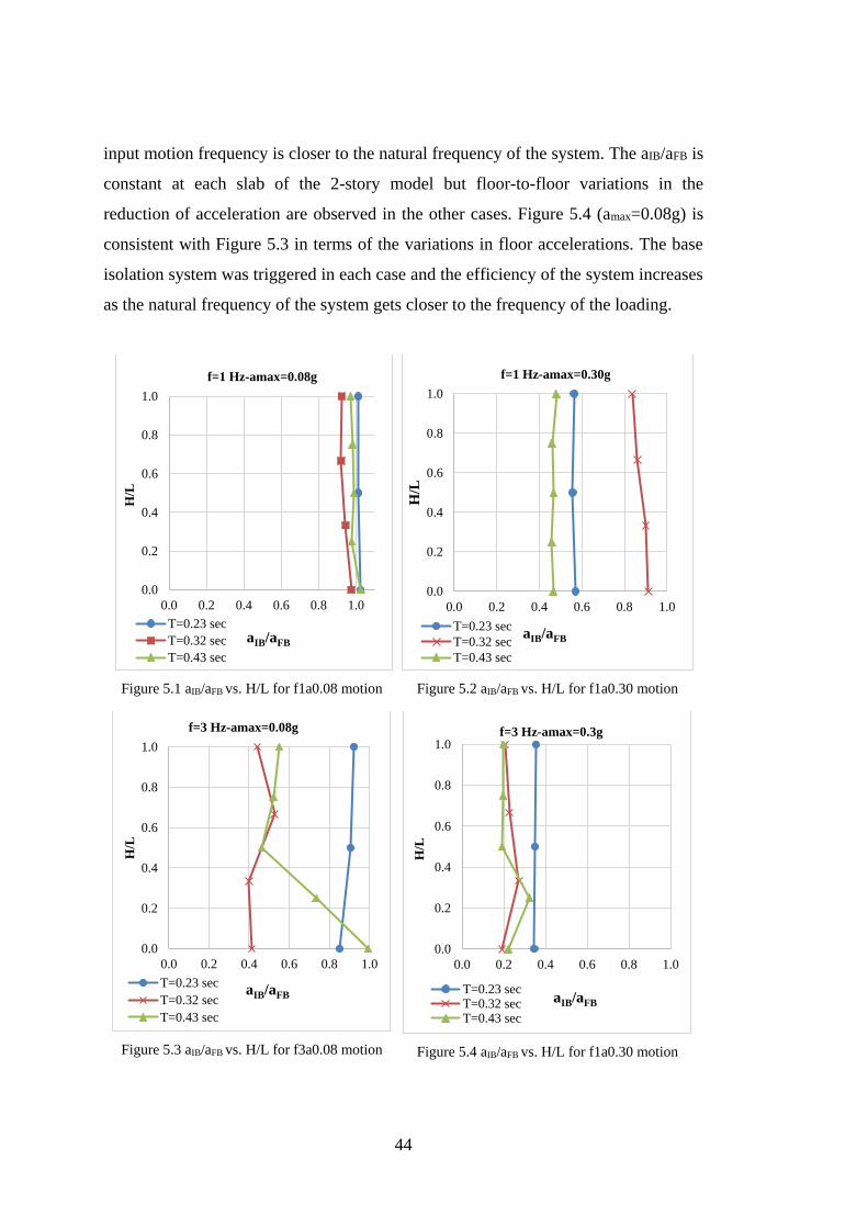
44
input motion frequency is closer to the natural frequency of the system. The aIB/aFB is
constant at each slab of the 2-story model but floor-to-floor variations in the
reduction of acceleration are observed in the other cases. Figure 5.4 (amax=0.08g) is
consistent with Figure 5.3 in terms of the variations in floor accelerations. The base
isolation system was triggered in each case and the efficiency of the system increases
as the natural frequency of the system gets closer to the frequency of the loading.
Figure 5.1 aIB/aFB vs. H/L for f1a0.08 motion
Figure 5.2 aIB/aFB vs. H/L for f1a0.30 motion
Figure 5.3 aIB/aFB vs. H/L for f3a0.08 motion
Figure 5.4 aIB/aFB vs. H/L for f1a0.30 motion
0.0
0.2
0.4
0.6
0.8
1.0
0.0 0.2 0.4 0.6 0.8 1.0
H/L
aIB/aFB
f=1 Hz-amax=0.08g
T=0.23 sec
T=0.32 sec
T=0.43 sec
0.0
0.2
0.4
0.6
0.8
1.0
0.0 0.2 0.4 0.6 0.8 1.0
H/L
aIB/aFB
f=1 Hz-amax=0.30g
T=0.23 sec
T=0.32 sec
T=0.43 sec
0.0
0.2
0.4
0.6
0.8
1.0
0.0 0.2 0.4 0.6 0.8 1.0
H/L
aIB/aFB
f=3 Hz-amax=0.08g
T=0.23 sec
T=0.32 sec
T=0.43 sec
0.0
0.2
0.4
0.6
0.8
1.0
0.0 0.2 0.4 0.6 0.8 1.0
H/L
aIB/aFB
f=3 Hz-amax=0.3g
T=0.23 secT=0.32 secT=0.43 sec
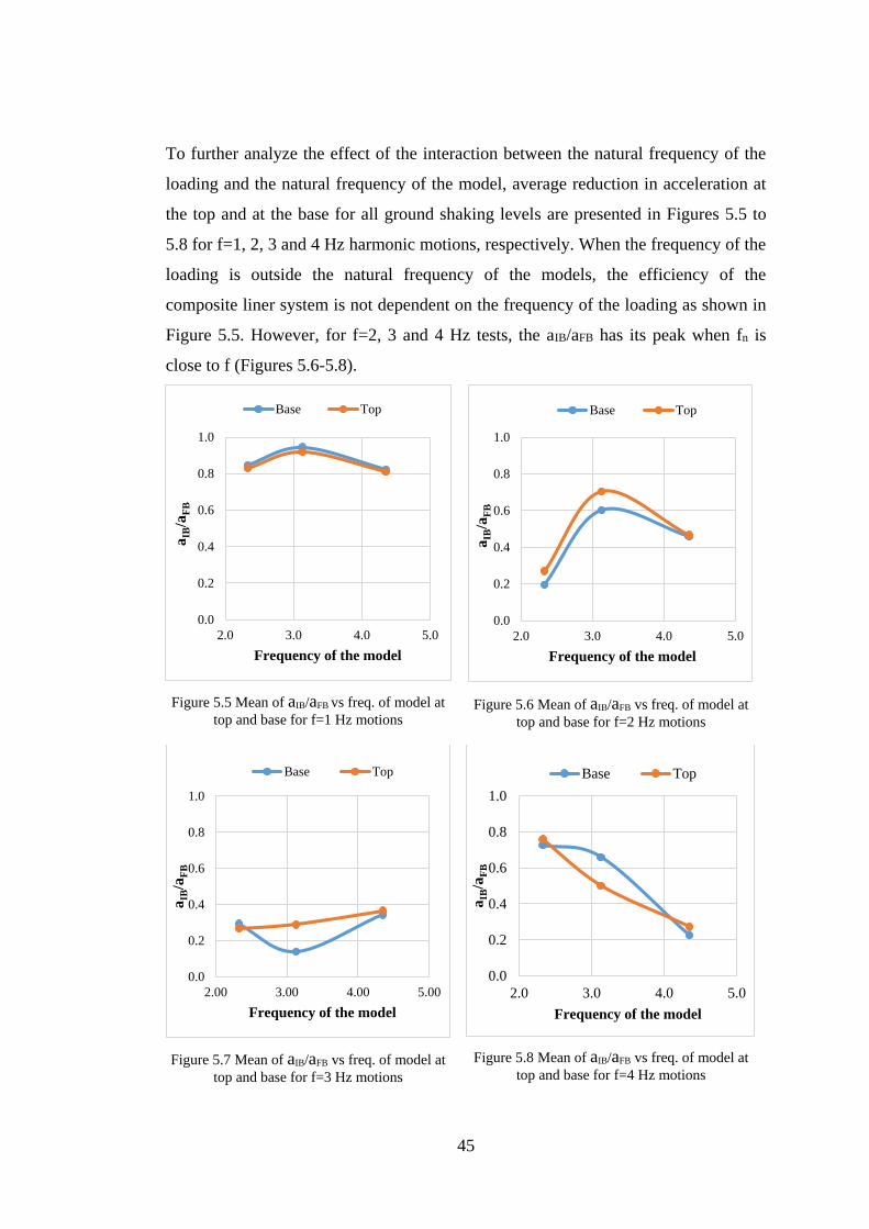
45
To further analyze the effect of the interaction between the natural frequency of the
loading and the natural frequency of the model, average reduction in acceleration at
the top and at the base for all ground shaking levels are presented in Figures 5.5 to
5.8 for f=1, 2, 3 and 4 Hz harmonic motions, respectively. When the frequency of the
loading is outside the natural frequency of the models, the efficiency of the
composite liner system is not dependent on the frequency of the loading as shown in
Figure 5.5. However, for f=2, 3 and 4 Hz tests, the aIB/aFB has its peak when fn is
close to f (Figures 5.6-5.8).
Figure 5.5 Mean of aIB/aFB vs freq. of model at
top and base for f=1 Hz motions
Figure 5.6 Mean of aIB/aFB vs freq. of model at
top and base for f=2 Hz motions
Figure 5.7 Mean of aIB/aFB vs freq. of model at
top and base for f=3 Hz motions
Figure 5.8 Mean of aIB/aFB vs freq. of model at
top and base for f=4 Hz motions
0.0
0.2
0.4
0.6
0.8
1.0
2.0 3.0 4.0 5.0
aIB
/aF
B
Frequency of the model
Base Top
0.0
0.2
0.4
0.6
0.8
1.0
2.0 3.0 4.0 5.0
aIB
/aF
B
Frequency of the model
Base Top
0.0
0.2
0.4
0.6
0.8
1.0
2.00 3.00 4.00 5.00
aIB
/aF
B
Frequency of the model
Base Top
0.0
0.2
0.4
0.6
0.8
1.0
2.0 3.0 4.0 5.0
aIB
/aF
B
Frequency of the model
Base Top

46
5.2 Comparison of Test Results for Ground Motions
Similar to the tests with the harmonic motions, the ratio of the absolute maximum
value of the measured accelerations in IB and FB conditions at each floor (aIB/aFB) is
plotted vs. H/L ratio for different models under the same ground motions. Two cases-
the ground motions from Landers and Loma Prieta earthquakes for different ground
shaking levels are provided in Figures 5.9 to 5.14. These plots are not similar to
Figures 5.1-5.4 since the interaction between the natural frequency of the model and
the predominant frequency of the ground motion are not substantial for real ground
motions. The aIB/aFB is approximately equal to one at the base for each model and the
efficiency of the composite liner system increases as the ground shaking level
increases. Floor accelerations at the 2-story (blue lines) and 3-story (red lines)
models are similar in each plot whereas, the maximum reduction in the floor
acceleration is generally observed at the middle floors of the 4-story model (green
lines).
When compared to the test results with harmonic motions (Figures 5.1-5.4), the
reduction in the maximum accelerations at the base in the tests with ground motions
(Figures 5.9-5.14) is systematically smaller even if the isolation system was triggered
for that particular test. To understand the impact in other spectral accelerations, the
average normalized response spectra measured at the base in FB and IB conditions in
2, 3 and 4-story models are compared for each ground motion through Figures 5.15
to 5.20 separately for reverse and strike slip earthquakes. These figures indicate that:
i) the average normalized spectra in IB conditions are almost always smaller than the
average normalized spectra in FB conditions (especially in the large period range), ii)
the mechanism of the earthquake does not have a noteworthy effect on the efficiency
of the base isolation system, and iii) behavior of the 2-story, 3-story and 4-story
models are not significantly different. Therefore, average normalized spectra for
different mechanism events can be combined for a better understanding in the
efficiency in the reduction of accelerations as shown in Figure 5.21, 5.22 and 5.23
for 2-story, 3-story and 4-story models, respectively. According to Figure 5.23, the
normalized spectral accelerations in FB and IB conditions are very close to each
other for 2-story model. Still, the normalized spectral accelerations decreased from
2.24 to 1.60 (≈28%) at the first mode natural period of the tested model.
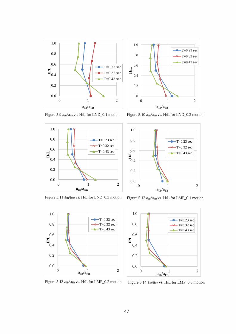
47
Figure 5.9 aIB/aFB vs. H/L for LND_0.1 motion
Figure 5.10 aIB/aFB vs. H/L for LND_0.2 motion
Figure 5.11 aIB/aFB vs. H/L for LND_0.3 motion
Figure 5.12 aIB/aFB vs. H/L for LMP_0.1 motion
Figure 5.13 aIB/aFB vs. H/L for LMP_0.2 motion
Figure 5.14 aIB/aFB vs. H/L for LMP_0.3 motion
0.0
0.2
0.4
0.6
0.8
1.0
0 1 2
H/L
aIB/aFB
T=0.23 sec
T=0.32 sec
T=0.43 sec
0.0
0.2
0.4
0.6
0.8
1.0
0 1 2
H/L
aIB/aFB
T=0.23 sec
T=0.32 sec
T=0.43 sec
0.0
0.2
0.4
0.6
0.8
1.0
0 1 2
H/L
aIB/aFB
T=0.23 sec
T=0.32 sec
T=0.43 sec
0.0
0.2
0.4
0.6
0.8
1.0
0 1 2
H/L
aIB/aFB
T=0.23 sec
T=0.32 sec
T=0.43 sec
0.0
0.2
0.4
0.6
0.8
1.0
0 1 2
H/L
aIB/aFB
T=0.23 sec
T=0.32 sec
T=0.43 sec
0.0
0.2
0.4
0.6
0.8
1.0
0 1 2
H/L
aIB/aFB
T=0.23 sec
T=0.32 sec
T=0.43 sec
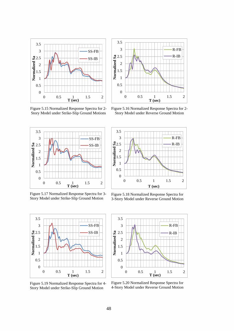
48
Figure 5.15 Normalized Response Spectra for 2-
Story Model under Strike-Slip Ground Motions
Figure 5.16 Normalized Response Spectra for 2-
Story Model under Reverse Ground Motion
Figure 5.17 Normalized Response Spectra for 3-
Story Model under Strike-Slip Ground Motion
Figure 5.18 Normalized Response Spectra for
3-Story Model under Reverse Ground Motion
Figure 5.19 Normalized Response Spectra for 4-
Story Model under Strike-Slip Ground Motion
Figure 5.20 Normalized Response Spectra for
4-Story Model under Reverse Ground Motion
0
0.5
1
1.5
2
2.5
3
3.5
0 0.5 1 1.5 2
No
rma
lize
d S
a
T (sec)
SS-FB
SS-IB
0
0.5
1
1.5
2
2.5
3
3.5
0 0.5 1 1.5 2
No
rma
lize
d S
a
T (sec)
R-FB
R-IB
0
0.5
1
1.5
2
2.5
3
3.5
0 0.5 1 1.5 2
No
rma
lize
d S
a
T (sec)
SS-FB
SS-IB
0
0.5
1
1.5
2
2.5
3
3.5
0 0.5 1 1.5 2
No
rma
lize
d S
a
T (sec)
R-FB
R-IB
0
0.5
1
1.5
2
2.5
3
3.5
0 0.5 1 1.5 2
No
rmali
zed
Sa
T (sec)
SS-FB
SS-IB
0
0.5
1
1.5
2
2.5
3
3.5
0 0.5 1 1.5 2
No
rmali
zed
Sa
T (sec)
R-FB
R-IB

49
Figure 5.21 Mean of Normalized Response Spectra for 2-Story Model under Strike-Slip and Reverse
Ground Motions
Figure 5.22 Mean of Normalized Response Spectra for 3-Story Model under Strike-Slip and
Reverse Ground Motions
Figure 5.23 Mean of Normalized Response Spectra for 4-Story Model under Strike-Slip and
Reverse Ground Motions
0
0.5
1
1.5
2
2.5
3
0 0.5 1 1.5 2 2.5 3 3.5 4
Sa
T (sec)
Mean-FB
Mean-IB
0
0.5
1
1.5
2
2.5
3
0 0.5 1 1.5 2 2.5 3 3.5 4
Sa
T (sec)
Mean-FB
Mean-IB
0
0.5
1
1.5
2
2.5
3
0 0.5 1 1.5 2 2.5 3 3.5 4
Sa
T (sec)
Mean-FB
Mean-IB
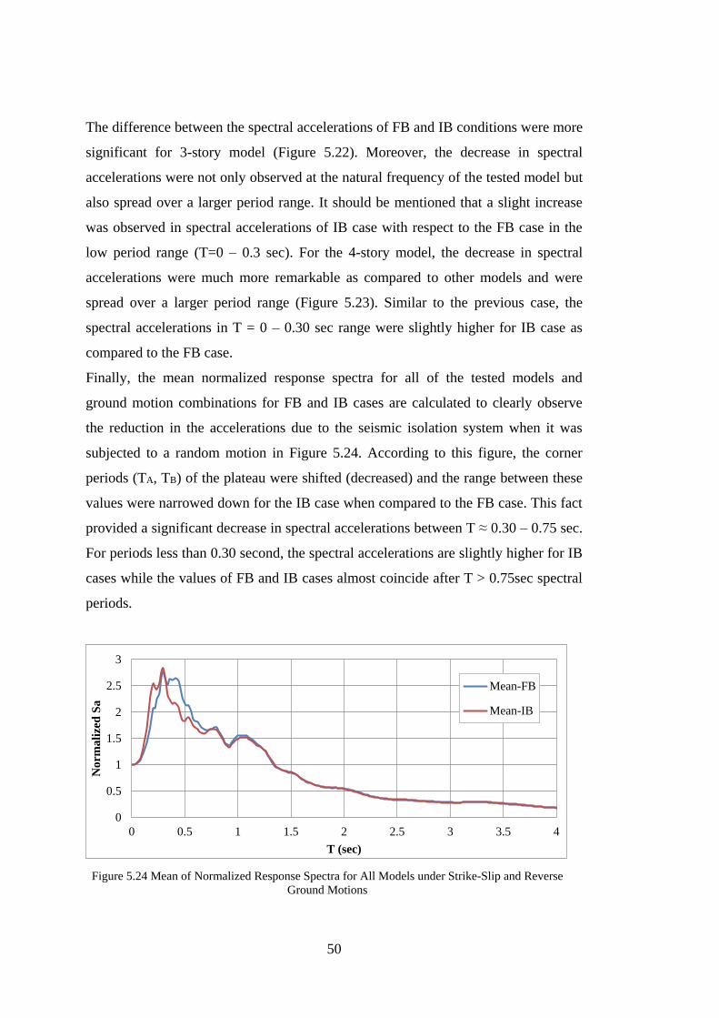
50
The difference between the spectral accelerations of FB and IB conditions were more
significant for 3-story model (Figure 5.22). Moreover, the decrease in spectral
accelerations were not only observed at the natural frequency of the tested model but
also spread over a larger period range. It should be mentioned that a slight increase
was observed in spectral accelerations of IB case with respect to the FB case in the
low period range (T=0 – 0.3 sec). For the 4-story model, the decrease in spectral
accelerations were much more remarkable as compared to other models and were
spread over a larger period range (Figure 5.23). Similar to the previous case, the
spectral accelerations in T = 0 – 0.30 sec range were slightly higher for IB case as
compared to the FB case.
Finally, the mean normalized response spectra for all of the tested models and
ground motion combinations for FB and IB cases are calculated to clearly observe
the reduction in the accelerations due to the seismic isolation system when it was
subjected to a random motion in Figure 5.24. According to this figure, the corner
periods (TA, TB) of the plateau were shifted (decreased) and the range between these
values were narrowed down for the IB case when compared to the FB case. This fact
provided a significant decrease in spectral accelerations between T ≈ 0.30 – 0.75 sec.
For periods less than 0.30 second, the spectral accelerations are slightly higher for IB
cases while the values of FB and IB cases almost coincide after T > 0.75sec spectral
periods.
Figure 5.24 Mean of Normalized Response Spectra for All Models under Strike-Slip and Reverse
Ground Motions
0
0.5
1
1.5
2
2.5
3
0 0.5 1 1.5 2 2.5 3 3.5 4
No
rmali
zed
Sa
T (sec)
Mean-FB
Mean-IB

51
The test results under modified and scaled ground motions are not as influenced by
the resonance effects as the tests results with harmonic motions do since the
empirical ground motions contains a large range of frequencies. When the test results
from all three models are combined, a significant reduction in spectral accelerations
between T ≈ 0.30 – 0.75 sec are observed. To model this reduction, the design
envelope recommended in Turkish Earthquake Code (TEC, 2007) was taken as a
reference point (Figure 5.25) and the necessary parts were modified to make it fit
better to mean spectra for FB and IB cases as shown in Figures 5.26 and 5.27. For
FB case, the formulation given in TEC (2007) was directly used with the same corner
periods (TA = 0.25 sec and TB = 0.45 sec) (Figure 5.26 and Equations 5.1-5.4). For
IB case, the characteristic periods obtained for the FB case were scaled by 0.75
(Equations 5.5-5.8) and a slight modification was made for T > TB (Figure 5.27). The
idealized response spectra for FB and IB cases are compared in Figure 5.28.
Figure 5.25 Special Design Acceleration Spectra According to Turkish Earthquake Code 2007

52
Figure 5.26 Fitted curve to Mean of Normalized Response Spectra for All Models in FB Condition
Figure 5.27 Fitted curve to Mean of Normalized Response Spectra for All Models in IB Condition
For FB condition:
45.025.0 ,, FBBFBA TT (5.1)
)0(5.11)( ,
,
FBA
FBA
TTT
TTS (5.2)
)(5.2)( ,, FBBFBA TTTTS (5.3)
)(5.2)( ,
8.0
,
FBB
FBBTT
T
TTS
(5.4)
0
0.5
1
1.5
2
2.5
3
0 0.5 1 1.5 2 2.5 3 3.5 4
Sa
T (sec)
Mean-FB
FB-fit
0
0.5
1
1.5
2
2.5
3
0 0.5 1 1.5 2 2.5 3 3.5 4
Sa
T (sec)
Mean-IB
IB-fit

53
For IB condition:
FBBIBBFBAIBA TTTT ,,,, .75.0.75.0 (5.5)
)0(5.11)( ,
,
IBA
IBA
TTT
TTS (5.6)
)(5.2)( ,, IBBIBA TTTTS (5.7)
)(5.2)( ,
7.0
,
IBB
IBBTT
T
TTS
(5.8)
Figure 5.28 Fitted Curves for Mean of Normalized Response Spectra for FB and IB conditions
0
0.5
1
1.5
2
2.5
3
0 0.2 0.4 0.6 0.8 1 1.2 1.4 1.6 1.8 2
Sa
T (sec)
IB-fit
FB-fit

54

55
CHAPTER 6
SUMMARY AND CONCLUSIONS
Within the content of this study, a 3-story building model is designed and tested by
employing harmonic and real/modified ground motions in the shaking table test set-
up that is located in the Soil Mechanics Laboratory of Middle East Technical
University. One of the main objectives is to analyze the seismic response of the
model in fixed based (where the model is fixed to the shaking table) and isolated
base (where the model is allowed to move over the composite liner system designed
as a base isolation system) conditions. Therefore, tests are repeated in these altered
base conditions using harmonic ground motions with different frequencies and
amplitudes. Since the interaction between the natural frequency of the system and the
frequency of the harmonic motion was found to be profound in the previous attempts
(similar 2-story and 4-story models were tested by Kalpakcı, 2013), special attention
was given to the natural frequency of the model. Model dimensions were modified in
a trial-and-error process to achieve a natural frequency around 3 Hz, which lies in the
middle of the frequency range of previous models. To reduce the effect of selected
frequency of harmonic motion on the response of the model, real acceleograms that
are richer in frequency content are also employed in the tests.
One of the main findings of Kalpakcı (2013) was related to the cut-off or triggering
amplitude of the ground motion: when the ground shaking levels are smaller than a
certain level, the composite liner system was found to be ineffective in reducing the
floor accelerations. This behavior is also observed in the experiments with harmonic
and real ground motions that were conducted in this study. The minimum threshold
acceleration, which is the minimum value necessary to trigger the base isolation
system, was measured to be around at ≈ 0.08g by Kalpakcı (2013); that is consistent
with the value stated in Yegian and Kadakal (2004) for rigid models. However, this
value was measured as low as at ≈ 0.03g in this study for 3Hz motion frequency. This
difference is attributed to the fact that the model was nearly in resonance during

56
shaking for 3Hz input motion frequency since the first-mode natural frequency of the
model is 3.13Hz.
One of the major findings of this study is related to the interaction between the
natural frequency of the loading and the natural frequency of the model. When the
frequency of the harmonic loading is away from the natural frequency of the models,
the efficiency of the composite liner system is not dependent on the frequency of the
harmonic loading. But when these two frequencies are close to each other, the
seismic isolation system became more efficient, especially in the tests with harmonic
motions. A function which defines the reduction in the floor accelerations provided
by the composite liner system based on the natural frequency of the superstructure
and the input motion frequency of the harmonic loading cannot be derived since the
system’s behavior is rather influenced by the resonance effects. Additionally, the
system was not triggered for some of the motions and higher modes of shaking were
observed in some of the experiments. By combining the results of tests with scaled
ground motions the efficiency of the composite liner system in reducing the spectral
accelerations in a range of frequencies were evaluated and a mean response spectra
was derived to define the behavior of the isolation system under ground motion
excitation
Since this experiments use models with different scales in dimension and weight
when compared to the real structures, test results presented here is only a preliminary
evaluation of the efficiency of geotextiles / geomembrane interface as base isolation.
For further experimental studies, the size and edge effects might be investigated by
testing different sizes of small blocks beneath the foundation. Also, analytical
calculations could be performed and compared in order to verify the results of these
experiments.

57
REFERENCES
Akkar S, Kale Ö, Yenier E, Bommer JJ. (2011). The high-frequency limit of usable
response spectral ordinates from filtered analogue and digital strong-motion
accelerograms. Earthq Eng Struct Dyn., 40(12):1387-1401.
doi:10.1002/eqe.1095.
Chiou, B., Darragh, R., Gregor, N., and Silva, W. (2008). “NGA Project Strong-
Motion Database,” Earthq. Spectra 24, 23-44.
Douglas J, Boore DM. (2010). High-frequency filtering of strong-motion records.
Bull Earthq Eng.,9(2):395-409. doi:10.1007/s10518-010-9208-4.
Kalpakcı, V. (2013). Seismic Isolation of Foundations by Composite Liners. Middle
East Technical University, PhD Dissertation.
Kalpakcı, V. (2015). Utilization of Geosynthetic Material Interfaces for Reduction of
Cyclic Motion Induced Accelerations. Adv Mater Res.;1105:361-364.
doi:10.4028/www.scientific.net/AMR.1105.361.
Naeim F, Mayes R (2001). Chapter 14 Design of Structure with Seismic Isolation.
In: The Seismic Design Handbook. Boston, MA: Springer US;.
doi:10.1007/978-1-4615-1693-4.
SeismoSignal v5.1.2 and SeismoSignal v2016, Seismosoft Ltd, available from:
http://seismosoft.com/seismosignal
SeismoSpect v2.1.2 and SeismoSpect v2016, Seismosoft Ltd, available from:
http://seismosoft.com/seismospect
SAP2000 Software v14, Computers and Structures, Inc. (CSI), available from:
https://www.csiamerica.com/products/sap2000
Turkish Earthquake Code (2007) Specification for structures to be built in disaster
areas. Ministry of Public Works and Settlement, Ankara.
Yegian MK, Lahlaf AM. (1992). Dynamic Interface Shear Strength Properties of
Geomembranes and Geotextiles. J Geotech Eng., 118(5):760-779.
doi:10.1061/(ASCE)0733-9410(1992)118:5(760)
58
Yegian MK, Kadakal U, Catan M. (1999). Geosynthetics for Earthquake Hazard
Mitigation. In: Geosynthetics ’99: Specifying Geosynthetics and Developing
Design Details. https://trid.trb.org/view.aspx?id=657415
Yegian MK, Kadakal U. (2004). Foundation Isolation for Seismic Protection Using a
Smooth Synthetic Liner. J Geotech Geoenvironmental Eng.,130(11):1121-
1130. doi:10.1061/(ASCE)1090-0241(2004)130:11(1121).
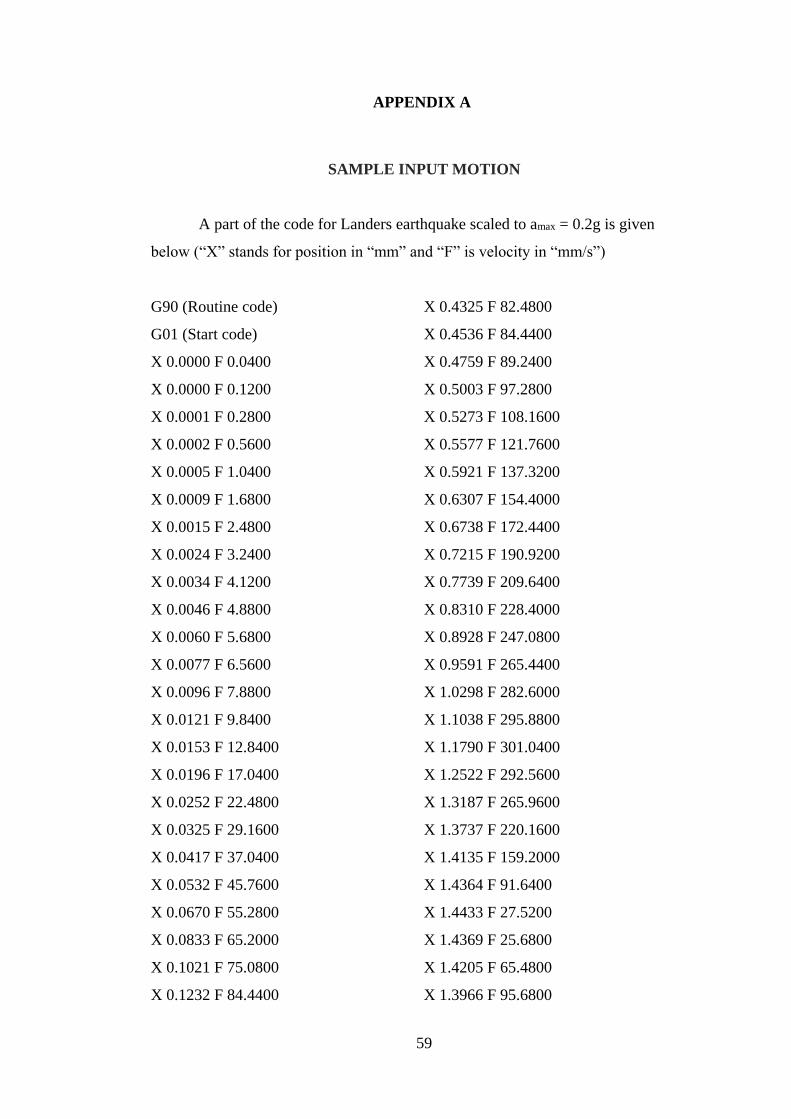
59
APPENDIX A
SAMPLE INPUT MOTION
A part of the code for Landers earthquake scaled to amax = 0.2g is given
below (“X” stands for position in “mm” and “F” is velocity in “mm/s”)
G90 (Routine code)
G01 (Start code)
X 0.0000 F 0.0400
X 0.0000 F 0.1200
X 0.0001 F 0.2800
X 0.0002 F 0.5600
X 0.0005 F 1.0400
X 0.0009 F 1.6800
X 0.0015 F 2.4800
X 0.0024 F 3.2400
X 0.0034 F 4.1200
X 0.0046 F 4.8800
X 0.0060 F 5.6800
X 0.0077 F 6.5600
X 0.0096 F 7.8800
X 0.0121 F 9.8400
X 0.0153 F 12.8400
X 0.0196 F 17.0400
X 0.0252 F 22.4800
X 0.0325 F 29.1600
X 0.0417 F 37.0400
X 0.0532 F 45.7600
X 0.0670 F 55.2800
X 0.0833 F 65.2000
X 0.1021 F 75.0800
X 0.1232 F 84.4400
X 0.4325 F 82.4800
X 0.4536 F 84.4400
X 0.4759 F 89.2400
X 0.5003 F 97.2800
X 0.5273 F 108.1600
X 0.5577 F 121.7600
X 0.5921 F 137.3200
X 0.6307 F 154.4000
X 0.6738 F 172.4400
X 0.7215 F 190.9200
X 0.7739 F 209.6400
X 0.8310 F 228.4000
X 0.8928 F 247.0800
X 0.9591 F 265.4400
X 1.0298 F 282.6000
X 1.1038 F 295.8800
X 1.1790 F 301.0400
X 1.2522 F 292.5600
X 1.3187 F 265.9600
X 1.3737 F 220.1600
X 1.4135 F 159.2000
X 1.4364 F 91.6400
X 1.4433 F 27.5200
X 1.4369 F 25.6800
X 1.4205 F 65.4800
X 1.3966 F 95.6800
60
X 0.1463 F 92.6000
X 0.1711 F 98.9600
X 0.1968 F 103.0400
X 0.2230 F 104.8400
X 0.2492 F 104.6400
X 0.2750 F 103.0000
X 0.3000 F 100.2800
X 0.3242 F 96.8400
X 0.3475 F 92.9600
X 0.3697 F 89.0400
X 0.3911 F 85.5600
X 0.4119 F 83.1200
X 1.3655 F 124.3600
X 1.3251 F 161.7200
X 1.2709 F 216.6000
X 1.1972 F 294.8400
X 1.0978 F 397.4000
X 0.9677 F 520.5200
X 0.8040 F 655.0800
X 0.6073 F 786.4000
X 0.3837 F 894.7600
X 0.1441 F 958.2800
X -0.0952 F 957.3600
X -0.3153 F 880.2400

61
APPENDIX B
PROPERTIES OF SHAKING TABLE AND MEASUREMETN DEVICES
Table B.1 Properties of shaking table used in METU soil laboratory
Table B.2 specification of data logger used in experiments

62
Table B.3 Specification of measurement devices used in experiments

63
APPENDIX C
GEOMEMBRANE AND GEOTEXTILE PROPERTIES
Table C.4 Material Properties of nonwoven heat-bonded Geotextile (Typar-3601)
PROPERTY TEST METHOD METRIC
Weight - Typical ASTM D-5261 203 g/sm
Tensile Strength ASTM D-4632 1,068 N
Elongation @ Break ASTM D-4632 60%
Puncture Strength ASTM D-4833 298 N
CBR Puncture ASTM D-6241 1,647 N
Trapezoidal Tear ASTM D-4533 400 N
Apparent Opening Size ASTM D-4751 0.10 mm
Permittivity ASTM D-4491 0.10 Sec-1
Water Flow Rate ASTM D-4491 611 l/min/sm
UV Resistance @ 500 Hours ASTM D-4355 70%
Table C.5 Physical and Mechanical Properties of UHMWPE Geomembrane (TIVAR 88-2)
Physical and Mechanical Properties Metric Comments
Specific Gravity 0.933 g/cc ASTM D792
Water Absorption <= 0.010 % Immersion, 24hr; ASTM D570(2)
Hardness, Shore D 64 ASTM D2240
Tensile Strength 37.9 MPa ASTM D638
Elongation at Break 200% ASTM D638
Tensile Modulus 0.669 GPa ASTM D638
Flexural Yield Strength 20.7 MPa ASTM D790
Flexural Modulus 0.724 GPa ASTM D790
Compressive Strength 20.0 MPa 10% Def.; ASTM D695
Compressive Modulus 0.552 GPa ASTM D695
Shear Strength 33.1 MPa ASTM D732
Izod Impact, Notched NB ASTM D256 Type A
Coefficient of Friction 0.08 Dry vs. Steel; QTM55007
Sand Slurry 11 1018 Steel = 100
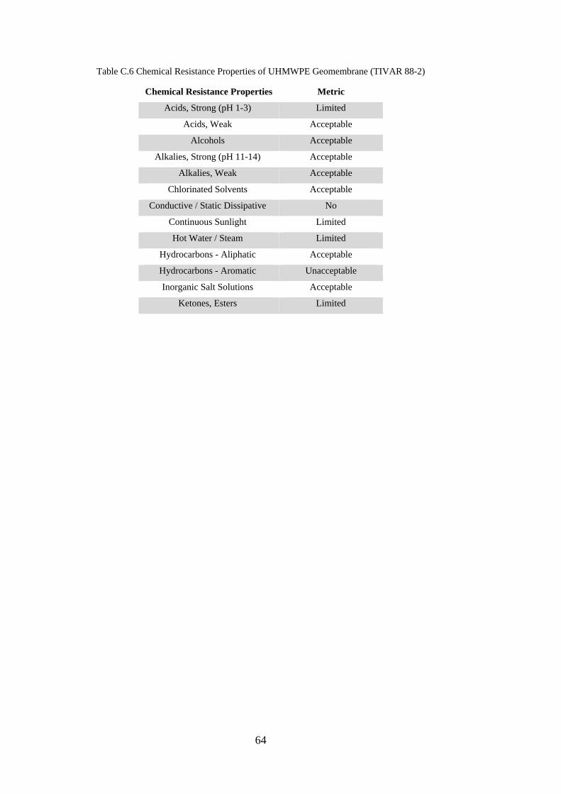
64
Table C.6 Chemical Resistance Properties of UHMWPE Geomembrane (TIVAR 88-2)
Chemical Resistance Properties Metric
Acids, Strong (pH 1-3) Limited
Acids, Weak Acceptable
Alcohols Acceptable
Alkalies, Strong (pH 11-14) Acceptable
Alkalies, Weak Acceptable
Chlorinated Solvents Acceptable
Conductive / Static Dissipative No
Continuous Sunlight Limited
Hot Water / Steam Limited
Hydrocarbons - Aliphatic Acceptable
Hydrocarbons - Aromatic Unacceptable
Inorganic Salt Solutions Acceptable
Ketones, Esters Limited

65
APPENDIX D
TIME HISTORIES OF INPUT GROUND MOTIONS
Figure D.1 Acceleration, velocity and displacement time histories for “Landers” ground motion scaled
to 0.1 g
-0.12
-0.08
-0.04
0
0.04
0.08
0.12
0 5 10 15 20 25 30 35
Acc
eler
ati
on
(g)
Time (s)
-200
-150
-100
-50
0
50
100
150
200
0 5 10 15 20 25 30 35
Vel
ocit
y (
mm
/s)
Time (s)
-60
-40
-20
0
20
40
60
80
0 5 10 15 20 25 30 35
Dis
pla
cem
ent
(mm
)
Time (s)

66
Figure D.2 Acceleration, velocity and displacement time histories for “Landers” ground motion scaled
to 0.2 g
-0.25-0.2
-0.15-0.1
-0.050
0.050.1
0.150.2
0 5 10 15 20 25 30 35
Acc
eler
ati
on
(g)
Time (s)
-400
-300
-200
-100
0
100
200
300
400
0 5 10 15 20 25 30 35
Vel
ocit
y (
mm
/s)
Times (s)
-150
-100
-50
0
50
100
150
0 5 10 15 20 25 30 35
Dis
pla
cem
ent
(mm
)
Time (s)
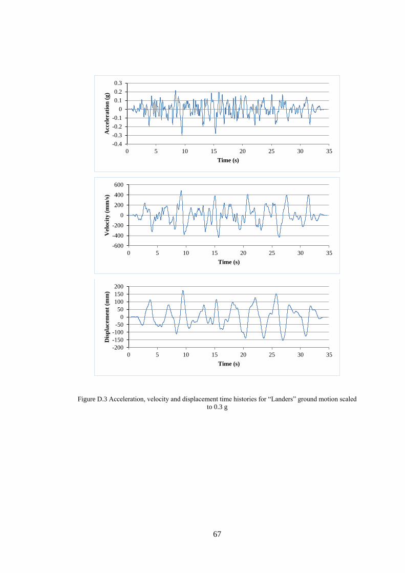
67
Figure D.3 Acceleration, velocity and displacement time histories for “Landers” ground motion scaled
to 0.3 g
-0.4
-0.3
-0.2
-0.1
0
0.1
0.2
0.3
0 5 10 15 20 25 30 35
Acc
eler
ati
on
(g)
Time (s)
-600
-400
-200
0
200
400
600
0 5 10 15 20 25 30 35
Vel
ocit
y (
mm
/s)
Time (s)
-200
-150
-100
-50
0
50
100
150
200
0 5 10 15 20 25 30 35
Dis
pla
cem
ent
(mm
)
Time (s)

68
Figure D.4 Acceleration, velocity and displacement time histories for “Chalfant Valley” ground
motion scaled to 0.1 g
-0.1-0.08-0.06-0.04-0.02
00.020.040.060.080.1
0 5 10 15 20 25 30 35 40
Acc
eler
ati
on
(g)
Time (s)
-200
-150
-100
-50
0
50
100
0 5 10 15 20 25 30 35 40
Vel
ocit
y (
mm
/s)
Time (s)
-30
-20
-10
0
10
20
30
40
0 5 10 15 20 25 30 35 40
Dis
pla
cem
ent
(mm
)
Time
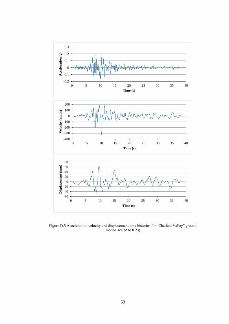
69
Figure D.5 Acceleration, velocity and displacement time histories for “Chalfant Valley” ground
motion scaled to 0.2 g
-0.2
-0.1
0
0.1
0.2
0.3
0 5 10 15 20 25 30 35 40
Acc
eler
ati
on
(g)
Time (s)
-400
-300
-200
-100
0
100
200
0 5 10 15 20 25 30 35 40
Vel
ocit
y (
mm
/s)
Time (s)
-60
-40
-20
0
20
40
60
80
0 5 10 15 20 25 30 35 40
Dis
pla
cem
ent
(mm
)
Time (s)
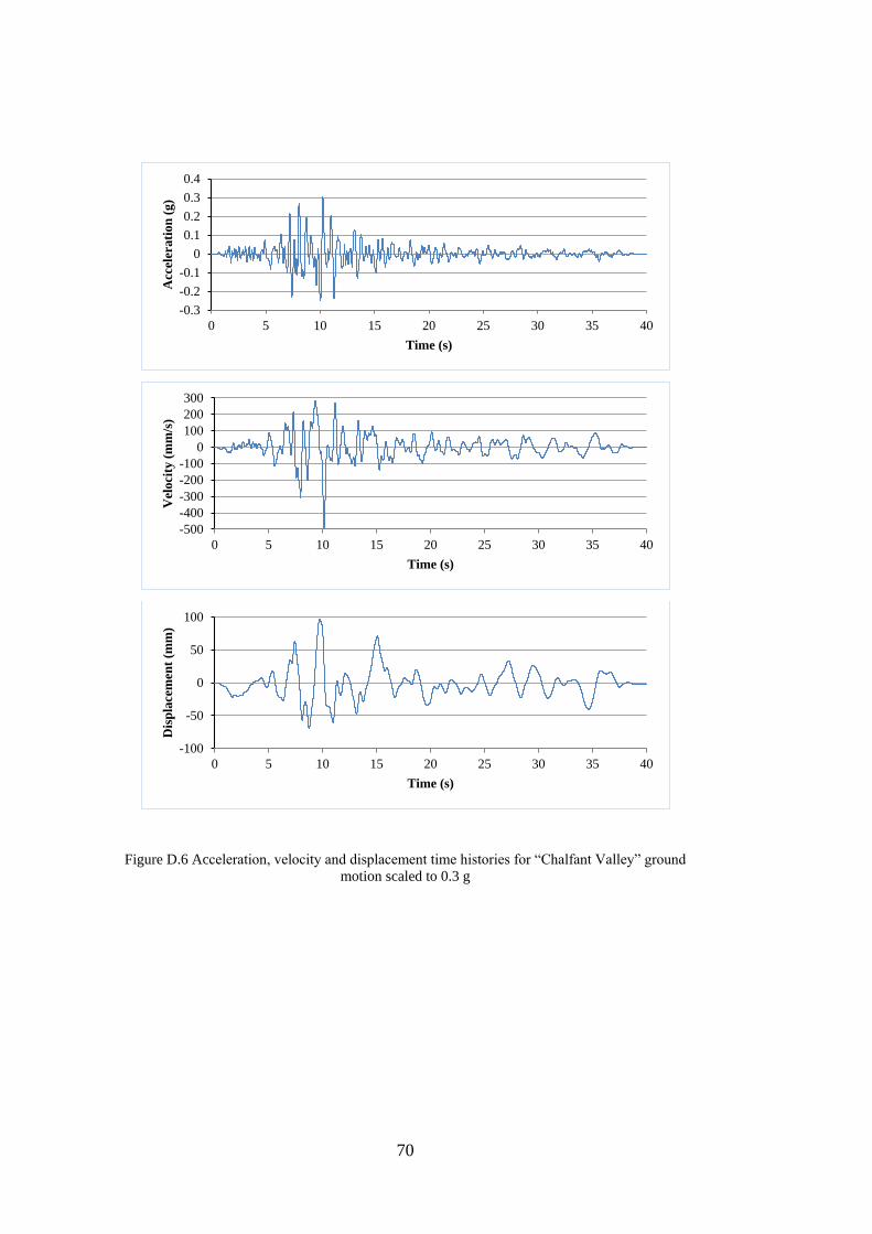
70
Figure D.6 Acceleration, velocity and displacement time histories for “Chalfant Valley” ground
motion scaled to 0.3 g
-0.3
-0.2
-0.1
0
0.1
0.2
0.3
0.4
0 5 10 15 20 25 30 35 40
Acc
eler
ati
on
(g)
Time (s)
-500
-400
-300
-200
-100
0
100
200
300
0 5 10 15 20 25 30 35 40
Vel
ocit
y (
mm
/s)
Time (s)
-100
-50
0
50
100
0 5 10 15 20 25 30 35 40
Dis
pla
cem
ent
(mm
)
Time (s)

71
Figure D.7 Acceleration, velocity and displacement time histories for “Loma Prieta” ground motion
scaled to 0.1 g
-0.15
-0.1
-0.05
0
0.05
0.1
0 5 10 15 20 25 30 35 40
Acc
eler
ati
on
(g)
Time (s)
-100
-50
0
50
100
0 5 10 15 20 25 30 35 40
Vel
ocit
y (
mm
/s)
Time (s)
-30
-20
-10
0
10
20
0 5 10 15 20 25 30 35 40
Dis
pla
cem
ent
(mm
)
Time (s)

72
Figure D.8 Acceleration, velocity and displacement time histories for “Loma Prieta” ground motion
scaled to 0.2 g
-0.3
-0.2
-0.1
0
0.1
0.2
0 5 10 15 20 25 30 35 40
Acc
eler
ati
on
(g)
Time (s)
-200
-150
-100
-50
0
50
100
150
200
0 5 10 15 20 25 30 35 40
Vel
ocit
y (
mm
/s)
Time (s)
-60
-40
-20
0
20
40
0 5 10 15 20 25 30 35 40
Dis
pla
cem
ent
(mm
)
Time (s)

73
Figure D.9 Acceleration, velocity and displacement time histories for “Loma Prieta” ground motion
scaled to 0.3 g
-0.4
-0.3
-0.2
-0.1
0
0.1
0.2
0.3
0 5 10 15 20 25 30 35 40
Acc
eler
ati
on
(g)
Time (s)
-300
-200
-100
0
100
200
300
0 5 10 15 20 25 30 35 40
Vel
ocit
y (
mm
/s)
Time (s)
-80
-60
-40
-20
0
20
40
60
0 5 10 15 20 25 30 35 40
Dis
pla
cem
ent
(mm
)
Time (s)
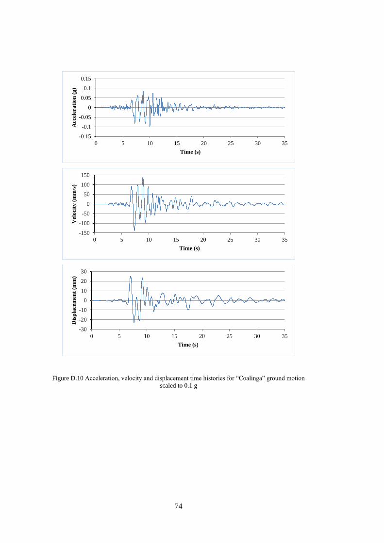
74
Figure D.10 Acceleration, velocity and displacement time histories for “Coalinga” ground motion
scaled to 0.1 g
-0.15
-0.1
-0.05
0
0.05
0.1
0.15
0 5 10 15 20 25 30 35
Acc
eler
ati
on
(g
)
Time (s)
-150
-100
-50
0
50
100
150
0 5 10 15 20 25 30 35
Vel
ocit
y (
mm
/s)
Time (s)
-30
-20
-10
0
10
20
30
0 5 10 15 20 25 30 35
Dis
pla
cem
ent
(mm
)
Time (s)

75
Figure D.11 Acceleration, velocity and displacement time histories for “Coalinga” ground motion
scaled to 0.2 g
-0.3
-0.2
-0.1
0
0.1
0.2
0.3
0 5 10 15 20 25 30 35 40
Acc
eler
ati
on
(g)
Time (s)
-300
-200
-100
0
100
200
0 5 10 15 20 25 30 35 40
Vel
ocit
y (
mm
/s)
Time (s)
-60
-40
-20
0
20
40
60
0 5 10 15 20 25 30 35 40
Dis
pla
cem
ent
(mm
)
Time (s)
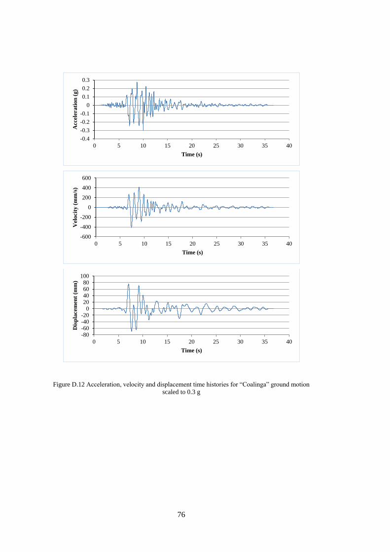
76
Figure D.12 Acceleration, velocity and displacement time histories for “Coalinga” ground motion
scaled to 0.3 g
-0.4
-0.3
-0.2
-0.1
0
0.1
0.2
0.3
0 5 10 15 20 25 30 35 40
Acc
eler
ati
on
(g)
Time (s)
-600
-400
-200
0
200
400
600
0 5 10 15 20 25 30 35 40
Vel
ocit
y (
mm
/s)
Time (s)
-80-60-40-20
020406080
100
0 5 10 15 20 25 30 35 40
Dis
pla
cem
ent
(mm
)
Time (s)
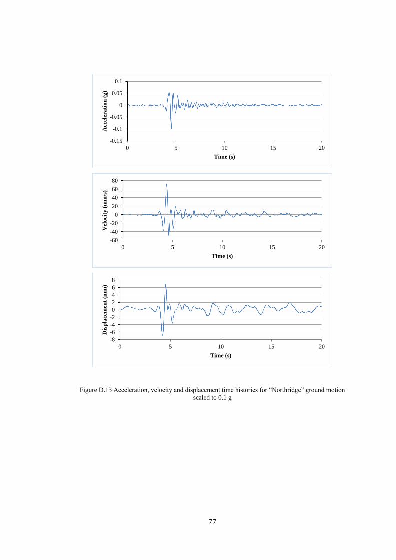
77
Figure D.13 Acceleration, velocity and displacement time histories for “Northridge” ground motion
scaled to 0.1 g
-0.15
-0.1
-0.05
0
0.05
0.1
0 5 10 15 20
Acc
eler
ati
on
(g)
Time (s)
-60
-40
-20
0
20
40
60
80
0 5 10 15 20
Vel
ocit
y (
mm
/s)
Time (s)
-8
-6
-4
-2
0
2
4
6
8
0 5 10 15 20
Dis
pla
cem
ent
(mm
)
Time (s)

78
Figure D.14 Acceleration, velocity and displacement time histories for “Northridge” ground motion
scaled to 0.2 g
-0.25
-0.2
-0.15
-0.1
-0.05
0
0.05
0.1
0.15
0 5 10 15 20
Acc
eler
ati
on
(g)
Time (s)
-150
-100
-50
0
50
100
150
0 5 10 15 20
Vel
ocit
y (
mm
/s)
Time (s)
-15
-10
-5
0
5
10
15
0 5 10 15 20
Dis
pla
cem
ent
(mm
)
Time (s)

79
Figure D.15 Acceleration, velocity and displacement time histories for “Northridge” ground motion
scaled to 0.3 g
-0.4
-0.3
-0.2
-0.1
0
0.1
0.2
0 5 10 15 20
Acc
eler
ati
on
(g)
Time (s)
-200
-100
0
100
200
300
0 5 10 15 20
Vel
ocit
y (
mm
/s)
Time (s)
-30
-20
-10
0
10
20
30
0 5 10 15 20
Dis
pla
cem
ent
(mm
)
Time (s)
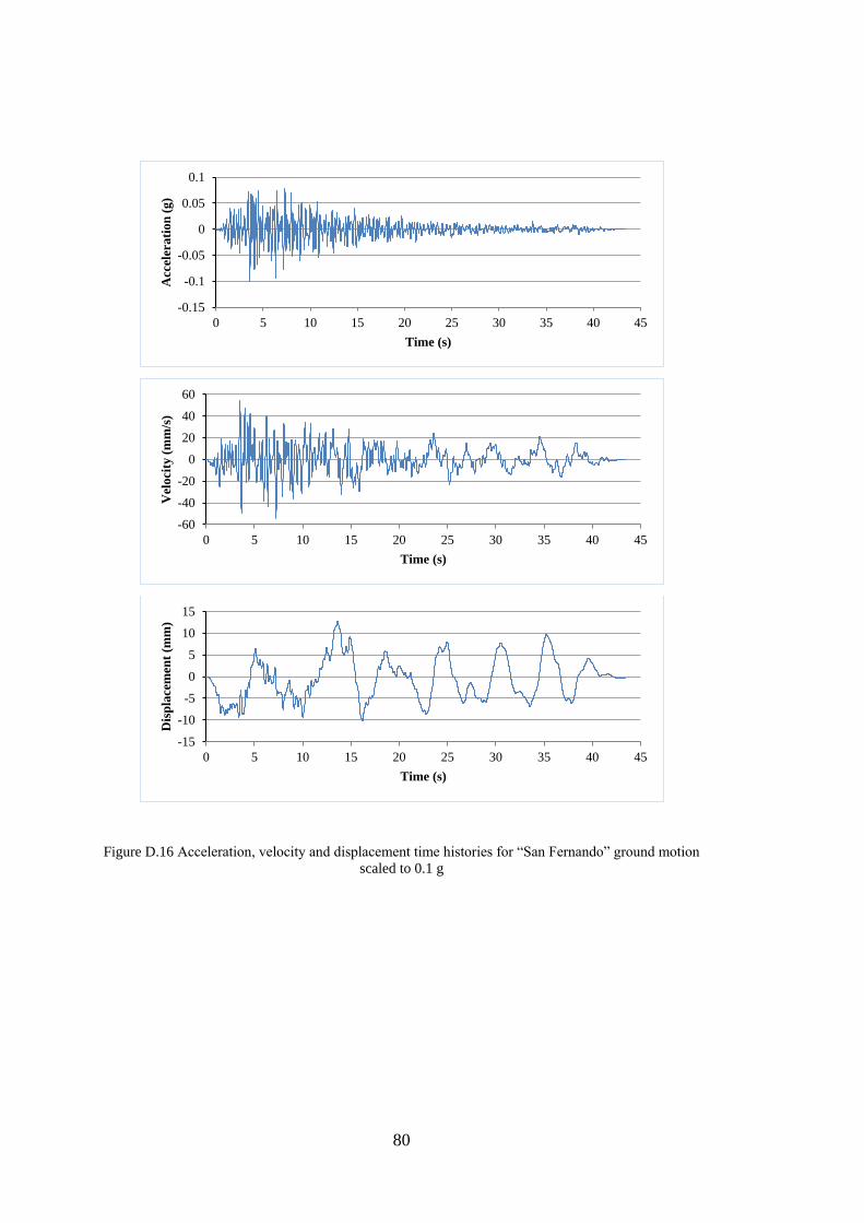
80
Figure D.16 Acceleration, velocity and displacement time histories for “San Fernando” ground motion
scaled to 0.1 g
-0.15
-0.1
-0.05
0
0.05
0.1
0 5 10 15 20 25 30 35 40 45
Acc
eler
ati
on
(g)
Time (s)
-60
-40
-20
0
20
40
60
0 5 10 15 20 25 30 35 40 45
Vel
ocit
y (
mm
/s)
Time (s)
-15
-10
-5
0
5
10
15
0 5 10 15 20 25 30 35 40 45
Dis
pla
cem
ent
(mm
)
Time (s)
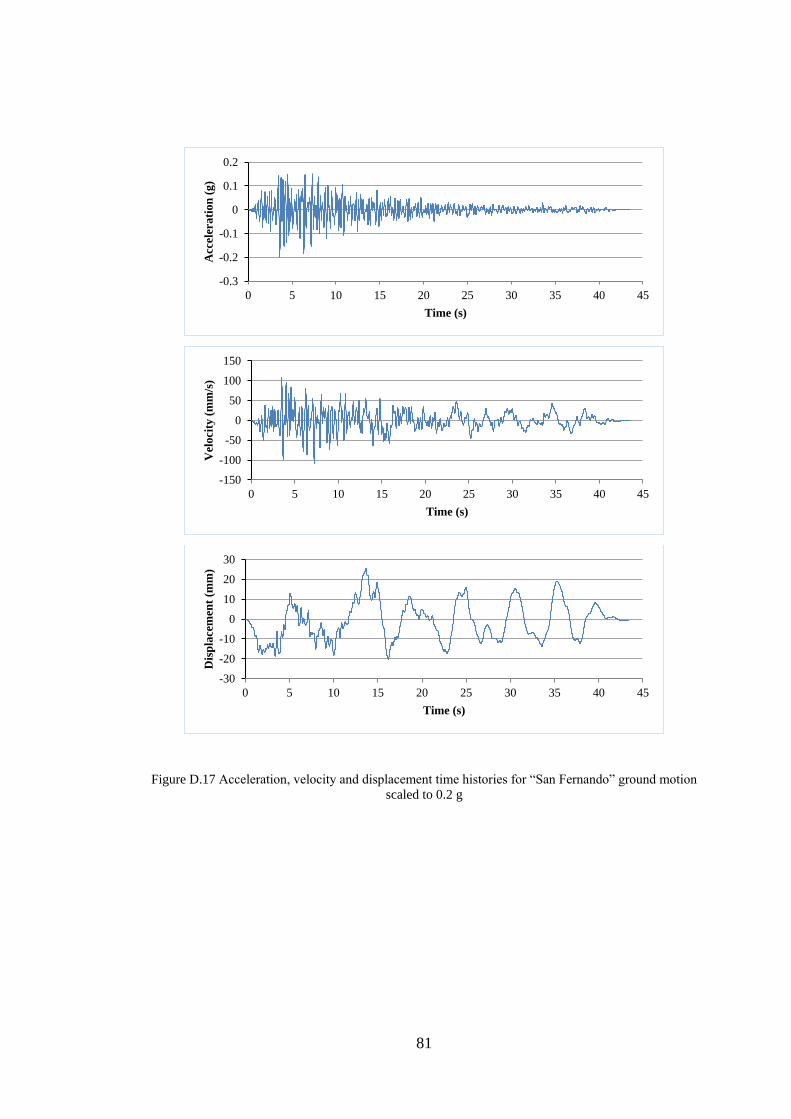
81
Figure D.17 Acceleration, velocity and displacement time histories for “San Fernando” ground motion
scaled to 0.2 g
-0.3
-0.2
-0.1
0
0.1
0.2
0 5 10 15 20 25 30 35 40 45
Acc
eler
ati
on
(g)
Time (s)
-150
-100
-50
0
50
100
150
0 5 10 15 20 25 30 35 40 45
Vel
ocit
y (
mm
/s)
Time (s)
-30
-20
-10
0
10
20
30
0 5 10 15 20 25 30 35 40 45
Dis
pla
cem
ent
(mm
)
Time (s)
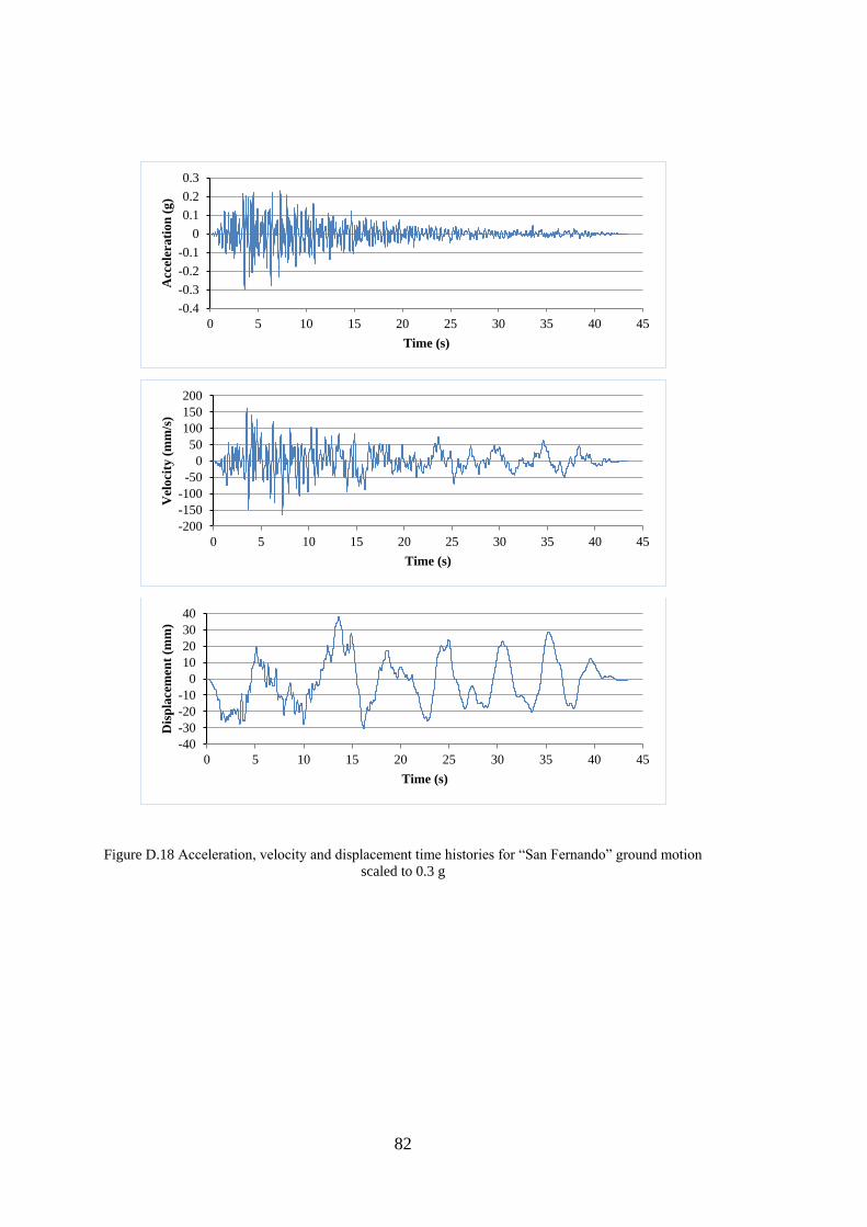
82
Figure D.18 Acceleration, velocity and displacement time histories for “San Fernando” ground motion
scaled to 0.3 g
-0.4
-0.3
-0.2
-0.1
0
0.1
0.2
0.3
0 5 10 15 20 25 30 35 40 45
Acc
eler
ati
on
(g)
Time (s)
-200
-150
-100
-50
0
50
100
150
200
0 5 10 15 20 25 30 35 40 45
Vel
ocit
y (
mm
/s)
Time (s)
-40
-30
-20
-10
0
10
20
30
40
0 5 10 15 20 25 30 35 40 45
Dis
pla
cem
ent
(mm
)
Time (s)