Experimental Design and Inferential Modeling in Pharmaceutical Crystallization

Timokleia Togkalidou and Richard D. Braatz Dept. of Chemical Engineering, University of Illinois at Urbana-Champaign, Urbana, IL 61801

Brian K. Johnson Dept. of Chemical Engineering, Princeton University, Princeton, NJ 08544

Omar Davidson and Arthur Andrews Merck. & Co., Inc., Whitehouse Station, NJ

A fractional factorial experimental design was used to investigate relative effects of operating conditions on the filtration resistance of a slurry produced in a pharmaceuti- cal semicontinuous batch cystallizer. The siu operating variables were seed type, seed amount, temperature, solvent ratio, addition time, and agitation intensity. An empirical model constructed between the operating variables and filtration resistance was used to define the factory operating procedure, which reduced filtration time 3.7-fold, Several chemometric techniques were used to construct inferential models between the in-pro- cess measurement of particle chord-length distribution and filtration resistance to help detect operational problems before completing the batch and decide when batch ciystal- lization runs should end. Depending on the model quality criterion, the most popular chemometric methods of partial least squares and top-down principal-component re- gression can produce lower quality models. Another chemometric approach, confi- dence-interval principal-component regression, predicted 70 % more accurately than the best OLS model. The main effects and inferential models serve different but comple- mentaiy roles in developing and implementing high-pei$omance ciystallization process operations. A main-effects model constructed from statistical experimental design data determined optimal operating conditions rapidly, while the inferential model can deter- mine operational problems and batch end times during batch-process operations.

Introduction

Crystallization from solution is an industrially important unit operation due to its ability to provide high purity separa- tions, which explains its predominant use in the pharmaceuti- cals industry. The crystal size distribution (CSD) is an impor- tant factor in the production of high-quality products and for determining the efficiency of downstream operations, such as filtration and washing. CSD-related characteristics of prod- uct crystals that have been optimized include mean crystal size (Ajinkya and Ray, 1974; Chang and Epstein, 1982; Jones, 19741, coefficient of variation (Chang and Epstein, 1982; Ma

Correspondence conccming this article should be addresaed to R. D. Braatz.

160 January 2001

et al., 19991, the ratio of the nucleated crystal mass to seed crystal mass (Chung et al., 1999; Mathews and Rawlings, 1998; Miller and Rawlings, 19941, and the crystal shape (Ma et al., 2000). An advantage of these objectives is their mathematical convenience, in that the objectives can be computed directly from the moments of the CSD.

The true objective for a pharmaceutical crystallization pro- cess may be to achieve sufficient product purity, to minimize the filtration time, or to achieve sufficient tablet stability when the crystals are mixed with crystals of other chemical species before forming the tablet. No reliable first-principles models are available for relating the CSD to these practical objec-

Vol. 47, No. 1 AIChE Journal

tives. The development of such models is especially challeng- ing for the crystals produced in the pharmaceutical industry, as these crystals often have a needle-like or more complex shape.

This motivates the use of statistical experimental design procedures to define optimal operating procedures for the crystallization of pharmaceutical chemicals, in which a true process objective is used as the goal of the optimization (John- son et al., 1997). In this study, an unbiased multivariable screening design of experiments led to a main-effects model that was followed by process optimization to minimize the filtration resistance, which was the primary variable of impor- tance for the industrial crystallizer of interest. A close inspec- tion of the crystallization process for a salt of an organic molecule that had a molecular weight of less than 1000 g/mol indicated six key input variables with respect to the output variable of interest, the filtration resistance. The optimized process was verified in the laboratory. A recommended fac- tory process was specified and successively demonstrated on the factory scale.

Another goal of this study was to construct a soft sensor (also known as an inferential model) to predict the filtration resistance in-process for the factory crystallizer. The purpose of the soft sensor was to aid in detecting operational prob- lems before the completion of the batch, and in deciding when batch crystallization runs should end, when the crystals are removed from the crystallizer and filtered. Chemometric techniques were applied to data collected from laboratory ex- periments to construct the soft sensor, which predicts filtra- tion resistance from a Lasentec focused-beam reflectance measurement (FBRM) instrument. This real-time in-process sensor, which obtains its information by laser backscattering, is rugged enough to be implemented on industrial crystalliz- ers.

The challenging aspect of the model construction is that the quantity of data is low relative to the model dimensional- ity. In our application, the chord-length distribution was rep- resented as a vector by binning the chord counts into 10 ranges of chord length. The number of experiments is 24. The data are highly collinear, so the model produced using ordinary least squares was too inaccurate to be useful. To address the collinearity, several chemometrics methods were used to construct inferential models, including partial least squares (PLS) and five different principal-component regres- sion (PCR) methods. It was found that the most commonly used chemometrics methods of PLS and top-down PCR may produce lower quality predictions than those produced by al- ternative PCR methods. More specifically, the chemometric technique known as confidence-interval PCR gave the tight- est prediction intervals.

Experimental Procedure The pharmaceutical product was a salt of an organic

molecule with molecular weight less than 1,000 g/mol. The product was crystallized in a baffled reactor, where the su- persaturation was created by adding a less efficient solvent that is miscible with the original solvent. Two streams, ace- tonitrile (product antisolvent) and toluene product concen- trate, were added simultaneously above the liquid surface at a constant rate to a seed bed of product. Each run was made

at the 40-g scale, with the final concentration between 38 and 41 g/L, for a total volume of one liter. Typical crystallizations produced a needle morphology with a length-to-width ratio greater than eight. Needle lengths reached 100 pm.

The relative effects of six input variables (operating condi- tions) on the main output variable, filtration resistance, were determined (Johnson et al., 1997). The input variables were the agitation intensity, seed type, seed amount, temperature, solvent ratio, and addition time. The output variables were filtration resistance (measured off-line) and particle chord- length distribution (measured in-process). Optical micro- graphs of the crystals were also taken.

The agitation speed was varied between 350 and 1450 rpm for a 62 mm diameter 45" pitched four-blade turbine in a 112-mm-dia. vessel. Each crystal slurry was agitated 2 h longer than the addition time of antisolvent. The seed amount (weight percentage, wt %) was based on the product in the starting concentrate. Seed was of two types: (1) final-product crystals that were dried and screened through a 20 mesh screen in a hammer mill and suspended in solvent, and ( 2 ) a stock supply of unfiltered slurry seed adjusted to the desired solvent ratio and 20 g/L starting concentration. Throughout each run, the temperature was held constant, and the con- centrate and antisolvent were charged in unison to maintain a constant solvent ratio.

Measurements of filtration resistance were obtained by fil- tering one-half of each crystallization slurry at 138 kPa on a 50-mm-dia. filter using a tight-weave multifilament polypropylene filter medium. Determination of the average specific cake resistance and the medium resistance was based upon the traditional filtration theory (Leu, 1986). All plots of average inverse filtrate rate vs. filtrate volume were linear, giving the average specific cake resistance from the slope of the curve and the medium resistance from the intercept. For easier interpretation of experimental data, the filtration time to collect 400 mL of filtrate was calculated based on the aver- age specific cake resistance and the medium resistance of each run. The remaining slurry was analyzed for particle chord- length distribution, which was measured in situ by an FBRM (model M300, version F) instrument. A chord length is a straight line between any two points on the edge of the parti- cle or particle structure (agglomerate). The FBRM counts hundreds of thousands of chords per second. This results in a number chord-length distribution (number of counts per sec- ond sorted by chord length). The chord-length distribution is sensitive to particle shape and particle population.

The chord-length distribution can be correlated with any upstream or downstream process variable that is a function of particle shape, dimension, and/or number of particles in the particle system. The primary chord-length distribution (number of counts per second sorted by chord length into bins) can be transformed by arithmetic manipulation to a weighted distribution. The weighted distributions that were used are the length-weighted distribution, the square- weighted distribution, and the cube-weighted distribution. There is a mean chord length associated with each of these distributions.

An optical micrograph of the crystals from each slurry at 200 x magnification was taken by a Zeiss optical microscope, model number ICM 405. Results were drawn by relating the optical micrographs with filtration times and the FBRM.

AIChE Journal January 2001 Vol. 47, No. 1 161

Theory Experimental design

Using statistical experimental design gives more disperse data for correlation, that is, the experiments are selected to more adequately cover the entire range of operations. This provides more confidence when scaling up the results to the factory. Covering a wide range of operations enables the soft sensor to predict the filtration resistance more reliably for a variety of crystal slurries. It is an important point that the data used to construct a soft sensor should not only be data collected during “best practices” or around the optimal oper- ating conditions, since a goal of the soft sensor is to provide accurate predictions even during abnormal operating condi- tions.

A multivariable one-eighth fractional factorial screening design of experiments was initially conducted to characterize the main effects of each input variable on the cake resistance and filtration time (Gunter, 1993). The screening design con- sisted of eight variable runs with two centerpoints.

It is an important point that the goal of this statistical ex- perimental design approach is to directly optimize the filtra- tion efficiency, whereas the goal of some other experimental design studies was to obtain improved estimates of the ki- netic parameters for crystal nucleation and growth (Chung et al., 2000; Mathews and Rawlings, 1998; Miller and Rawlings, 1994).

Chemometrics The strong correlations within the data make it impossible

to construct an accurate ordinary least-square (OLS) model between the filtration time and the entire chord-length distri- bution. Hence ordinary least squares was only applied to re- late the filtration time to certain characteristics of the chord- length distribution (such as mean chord length, fraction of small particles). The ability of the chemometric methods of PCR and PLS to handle highly correlated data allows these methods to construct inferential models based on the entire chord-length distribution.

The first step in PCR is to transform the input variables into a set of new variables, called principal components, which are uncorre- lated. The next step is to select as new variables a subset of the principal components that has a smaller dimensionality than the original input space. The last step is to perform or- dinary least-square regression of the principal components against the output. Five different methods were considered for selecting which principal components to include in the regression model:

Top-down selection PCR (TPCR) (Xie and Kalivas, 1997) Correlation PCR (CPCR) (Xie and Kalivas, 1997) Forward selection PCR 1 (FPCR1) (Draper and Smith,

Forward selection PCR 2 (FPCR2) (Xie and Kalivas,

Confidence interval PCR (CIPCR) The inferential model has the form

Principal-Component Regression Methods.

1981; Phatak et al., 1993)

1997)

y = x T b , (1)

where y is the output prediction, x is the vector of inputs, b is the vector of regression coefficients, and the data are as- sumed to be mean centered. The PCR method computes the regression coefficient from

where Y is the vector of outputs in the training set, X is the matrix of inputs in the training set, and the columns of V are the eigenvectors of X T X corresponding to the selected prin- cipal components. If all principal components were used, then the estimate would be the same as in ordinary least squares. Only a subset of the principal components can be used for regression due to high data collinearity and the small quan- tity of data relative to the number of regression coefficients.

The challenge then becomes to select the best principal components for use in the regression step. Top-down selec- tion, the most popular method for principal-component se- lection, assumes that the most informative principal compo- nents are the ones with the greatest variability, and then uses some criterion for deciding the number of principal compo- nents. However, the principal components with the highest variability may not be the most informative for the purpose of prediction, since this criterion does not contain any infor- mation on the correlation between each principal component and the output (Jackson, 1991; Jolliffe, 1982; Massy, 1965). In order to choose which of these principal components repre- sent better the correlation of the input to the output space, CPCR (Xie and Kalivas, 1997), FPCRl (Draper and Smith, 1981; Phatak et al., 1993), FPCR2 (Xie and Kalivas, 1997), and CIPCR have been proposed.

Since the other chemometrics methods have clear descrip- tions in other journal articles, only the CIPCR method will be described here. The CIPCR method is designed specifi- cally to give tight prediction intervals. CIPCR constructs con- fidence intervals for regression coefficients between the prin- cipal components and the output, and selects only those that are statistically significant. The significance is determined us- ing a hypothesis test based on the variance of the regression coefficients computed using standard statistical formula (Beck and Arnold, 1977).

Partial Least-Square Regression. The PLS method uses output data Y while it is constructing the new regression variables and thus eliminates the weight of variables with high variability but no relevance to the output space (Martens and Naes, 1989; Russell et al., 2000). Due to the nonlinear form of the PLS estimator, it is difficult to derive exact prediction intervals. An approximation on the prediction intervals can be constructed by linearization of the PLS estimator (Phatak et a]., 1993). The accuracy of the prediction intervals was comparable to Monte Carlo simulation for several data sets (Phatak et al., 1993).

The predictive ability of the model can be quantified by the relative ability of predic- tion (RAP) (Martens and Naes, 1989). The RAP is close to unity for perfect predictors, and is close to zero for very poor predictors. The mean value of the prediction interval is an- other property of interest that is used as a criterion to com- pare between the different methods (such as Faber and

Measures of Accuraq of Models.

162 January 2001 Vol. 47, No. 1 AIChE Journal

Kowalski, 1996; Jackson, 1991; Phatak et al., 1993, and cita- tions therein). All chemometric calculations were performed using home-grown MATLAB code, except for the PLS algo- rithm, in which the Matlab PLS Toolbox 2.0 was used (Wise and Gallagher, 1998).

Results Main eflects model

Based on the ten experiments (described in the Experi- mental Design section), an ordinary least-square model (often called a main effects model) was fit to correlate the filtration time to the six input variables. The model indicated that in order to reduce filtration time, the agitation speed and sol- vent ratio should be lowered, the temperature, seed amount, and addition time should be increased, and dried seed should be preferred over a slurry seed.

It was attempted to reduce filtration time by adjusting each input variable in the direction dictated by the main effects model of the screening design. Only the addition time was not optimized to shorten run times due to project time limi- tations.

The first optimization run, OPTl in Table 1, indeed pro- duced the second best filtration time of all the runs, 8.7 min. In order to verify the predictions of the main effects model, additional runs were made, changing one input variable of the optimized run, OPT1, to the negative of the design range. In all cases, except for seed type, switching only one variable to the negative of the optimum predicted by the screening resulted in an increase in filtration time. In addition, multi- ple inputs were changed to the negative of the optimum set- tings, run OPTNEG of Table 1, resulting in the third longest filtration time of all the runs, 99 min.

An empirical model to predict the filtration time of a dried seed run over the ranges evaluated in Table 1 was developed using first-order multivariable ordinary least-square regres- sion. The model was based on the 16 crystallization runs, in- cluding the optimization runs. The slurry seed runs were ex- cluded from the model to increase the model accuracy, as will be discussed below.

The prediction equation of filtration resistance from the five input variables (excluding seed type) is given by:

Time (mid to collect 400 mL of filtrate

34.5 + 0.0362 -(agitation intensity, = rpm)+21.47.(solvent ratio)- 1.77

- (temp., 'C) - 2.64 (charge time, h) - 0.722 -(seed amount, wt. %). (3)

With respect to the ranges studied, agitation intensity had the largest effect on the resulting filtration time of a crystal- lization, followed by solvent ratio, temperature, charge time, and seed amount.

A strong interaction between seed type and seed amount exists. The amount of seed had little effect when the dried seed was used, but if slurry seed was used, the amount of seed had a dramatic effect. The adverse combination of low seed amount and slurry seed led to the longest filtration times of all the runs, 191 min. Conversely, the best filtration time, 6.0 min, of all runs was experienced using 10 wt % slurry seed under favorable conditions for all the other variables, except addition time, similar to run OPTl in Table 1. It was our hypothesis that when there is not enough slurry seed, the crystallization system becomes starved for crystal surface area, resulting in a high supersaturation and significant nucleation. According to this hypothesis, we would expect to see a bi- modal distribution for crystals produced from crystallization runs with low slurry seed (this is confirmed in optical micro- graphs below). The dried seed was more desirable, due to the strong sensitivity of filtration time to the amount of slurry seed.

The difference in sensitivities for the dried and slurry seed is likely due to the different nature of the crystal surfaces. The surface of the dried seed is rough and fractured during the drying and milling process, which undoubtably results in a relatively large number of growth sites distributed across the surface even if the amount of dried seed is low. On the other hand, the slurry seed is quite intact, with a much smoother surface. Since the crystals grow in a needle-like shape, the growth sites for slurry seed are predominantly at the opposite ends of the longest length dimension of the crys- tal. When the quantity of slurry seed is low, the limited num-

Table 1. Experimental Design ~~~ ~~ ~~ ~~

Screening Previous Factory Recommended Design Range OPTl OPTNEG

Input variables Agitation intensity, rpm 350 to 1450 350 1450 1450 (tip speed) 900 Seed amount, wt. % of batch 3.0 to 10 10 3 5.3 10 Seed type Slurry or dried Dried Dried Dried Dried Temuerature. "C 15 to 25 25 16 18 24 Vol& ratio, MeCN:Tol 1:l to 2.33:l 1:l 2.33:l 1.66:l Charge time, h 3 to 9 3 3 6.9

1.22:l 6.9

Output variables Avg. specific cake resistance,

x lo-'". m/ka 290 to 8.5 12 150 Medium cake' resistance.

Filtration time,* min. x IO-"', I/m 62 to 3.2 7.9 36

Dried model orediction 8.8 98 Experimental result 191 to 6.0 8.7 99

89

12

57 68

35

11

23 25

*Filtration time for collecting 400 mL of filtrate

AIChE Journal January 2001 Vol. 47, No. 1 163

Figure 1. Optical micrograph (200 x 1; slowest filtration.

ber of growth sites results in an increase in supersaturation during the crystallization run, resulting in nucleation and the bimodal distribution of crystals.

Optical micrographs Optical micrographs confirmed an obvious bimodal distri-

bution of particles and fines existing in the two runs with the highest filtration resistance, which used slurry seed (see Fig-

Figure 3. Optical micrograph (200 x ); factory recom- mended.

ure 1). Conversely, optical micrographs confirmed that the lowest filtration resistance corresponded to cases where few fines existed and particles were of considerable size, 50-100 pm in length (Figures 2-4). Comparing the results in Table 2 with the optical micrographs, we can qualitatively correlate the properties of filtration time, the percentage of particles with chord length between 0.8 and 1.9 pm, and mean chord length with the crystal size distribution in the related images.

Figure 2. Optical micrograph (200 x 1; laboratory rec- ommended. Figure 4. Optical micrograph (200 x ); fastest filtration.

164 January 2001 Vol. 47, No. 1 AIChE Journal

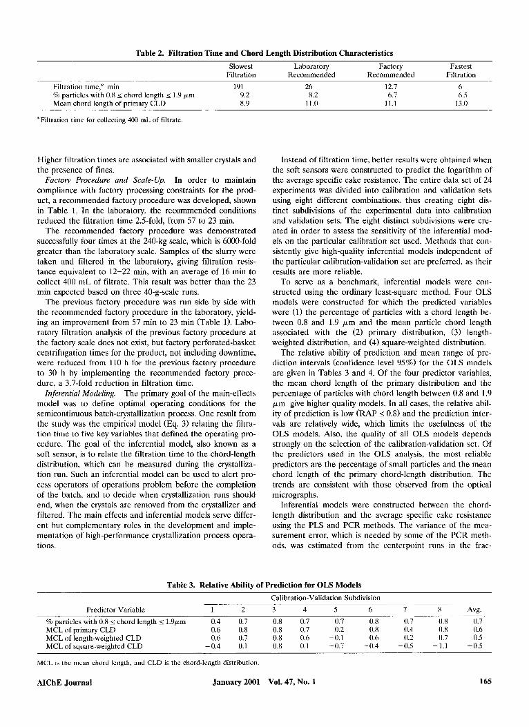
Table 2. Filtration Time and Chord Length Distribution Characteristics Slowest Laboratory Factory Fastest

Filtration Recommended Recommended Filtration

Filtration time,* rnin 191 26 % particles with 0.8 I chord length I 1.9 p m 9.2 8.2 Mean chord length of primary CLD 8.9 11.0

12.7 6 6.7 6.5

11.1 13.0

"Filtration time for collecting 400 mL of filtrate.

Higher filtration times are associated with smaller crystals and the presence of fines.

In order to maintain compliance with factory processing constraints for the prod- uct, a recommended factory procedure was developed, shown in Table I . In the laboratory, the recommended conditions reduced the filtration time 2.5-fold, from 57 to 23 min.

The recommended factory procedure was demonstrated successfully four times at the 240-kg scale, which is 6000-fold greater than the laboratory scale. Samples of the slurry were taken and filtered in the laboratory, giving filtration resis- tance equivalent to 12-22 min, with an average of 16 rnin to collect 400 mL of filtrate. This result was better than the 23 rnin expected based on three 40-g-scale runs.

The previous factory procedure was run side by side with the recommended factory procedure in the laboratory, yield- ing an improvement from 57 min to 23 rnin (Table 1). Labo- ratory filtration analysis of the previous factory procedure at the factory scale does not exist, but factory perforated-basket centrifugation times for the product, not including downtime, were reduced from 110 h for the previous factory procedure to 30 h by implementing the recommended factory proce- dure, a 3.7-fold reduction in filtration time.

The primary goal of the main-effects model was to define optimal operating conditions for the semicontinuous batch-crystallization process. One result from the study was the empirical model (Eq. 3) relating the filtra- tion time to five key variables that defined the operating pro- cedure. The goal of the inferential model, also known as a soft sensor, is to relate the filtration time to the chord-length distribution, which can be measured during the crystalliza- tion run. Such an inferential model can be used to alert pro- cess operators of operations problem before the completion of the batch, and to decide when crystallization runs should end, when the crystals are removed from the crystallizer and filtered. The main effects and inferential models serve differ- ent but complementary roles in the development and imple- mentation of high-performance crystallization process opera- tions.

Factory Procedure and Scale-Up.

Inferential Modeling.

Instead of filtration time, better results were obtained when the soft sensors were constructed to predict the logarithm of the average specific cake resistance. The entire data set of 24 experiments was divided into calibration and validation sets using eight different combinations, thus creating eight dis- tinct subdivisions of the experimental data into calibration and validation sets. The eight distinct subdivisions were cre- ated in order to assess the sensitivity of the inferential mod- els on the particular calibration set used. Methods that con- sistently give high-quality inferential models independent of the particular calibration-validation set are preferred, as their results are more reliable.

To serve as a benchmark, inferential models were con- structed using the ordinary least-square method. Four OLS models were constructed for which the predicted variables were (1) the percentage of particles with a chord length be- tween 0.8 and 1.9 p m and the mean particle chord length associated with the (2) primary distribution, (3) length- weighted distribution, and (4) square-weighted distribution.

The relative ability of prediction and mean range of pre- diction intervals (confidence level 95%) for the OLS models are given in Tables 3 and 4. Of the four predictor variables, the mean chord length of the primary distribution and the percentage of particles with chord length between 0.8 and 1.9 pm give higher quality models. In all cases, the relative abil- ity of prediction is low (RAP I 0.8) and the prediction inter- vals are relatively wide, which limits the usefulness of the OLS models. Also, the quality of all OLS models depends strongly on the selection of the calibration-validation set. Of the predictors used in the OLS analysis, the most reliable predictors are the percentage of small particles and the mean chord length of the primary chord-length distribution. The trends are consistent with those observed from the optical micrographs.

Inferential models were constructed between the chord- length distribution and the average specific cake resistance using the PLS and PCR methods. The variance of the mea- surement error, which is needed by some of the PCR meth- ods, was estimated from the centerpoint runs in the frac-

Table 3. Relative Ability of Prediction for OLS Models Calibration-Validation Subdivision

Predictor Variable 1 2 3 4 5 6 7 8 Avg.

% particles with 0.8 I chord length I 1.9pm 0.4 0.7 0.8 0.7 0.7 0.8 0.7 0.8 0.7 MCL of primary CLD 0.6 0.8 0.8 0.7 0.2 0.8 0.4 0.8 0.6 MCL of length-weighted CLD 0.6 0.7 0.8 0.6 -0.1 0.6 0.2 0.7 0.5 MCL of square-weighted CLD -0.4 0.1 -0.8 0.1 -0.7 -0.4 -0.5 -1.1 -0.5

MCL is the mean chord length, and CLD is the chord-length distribution.

AIChE Journal January 2001 Vol. 47, No. 1 165

Table 4. Mean Range of Prediction Intervals (Confidence Level 95%) for OLS Models Calibration-Validation Subdivision

Predictor Variable 1 2 3 4 5 6 7 8 Avg. % Particles with 0.8 5 chord length 5 1.9 prn 2.1 2.2 1.9 2.4 2.2 2.0 2.3 2.1 2.2 MCL of primary CLD 2.1 2.3 2.3 2.0 2.0 1.8 1.9 2.1 2.1 MCL of length-weighted CLD 2.5 2.5 3.1 2.1 2.2 2.3 2.2 2.7 2.5 MCL of square-weighted CLD 3.9 3.6 3.9 3.7 3.2 3.4 3.5 3.4 3.6

MCL is the mean chord length, and CLD is the chord-length distribution.

Table 5. Number of Predictor Variables

Calibration-Validation Subdivision 1 2 3 4 5 6 1 8 A v g .

TPCR 8 4 3 3 3 1 6 3 3.9 CPCR 3 2 3 1 3 2 4 4 2.8 FPCRl 4 2 1 3 2 3 3 2 2.5 FPCR2 4 4 4 2 5 3 3 4 3.6 CIPCR 4 3 1 3 2 3 6 2 3.0 PLS 5 4 1 2 6 1 5 3 3 . 4

tional factorial design of experiments. The data (particle chord-length distribution) were mean-centered before the construction of the predictors. The complete data set in- cluded 24 experiments, with 10 bins in the chord-length dis- tribution (number of predictor variables at the original space). The rank of the covariance matrix X T X was less than 10. The strong collinearity of the data and the relatively small number of experiments pose a challenging problem for con- structing a reliable and accurate predictor.

The number of predictor variables used in each chemomet- ric technique is reported in Table 5. On average, TPCR se- lects a large number of principal components than the other methods. The principal components selected as predictor variables in each PCR method are reported in Table 6. In almost all cases the alternative PCR methods do not include the second or fourth principal components in constructing the inferential models. The implication is that the second and fourth principal components are not strongly correlated to the predicted output (logarithm of the filtration resistance). In fact, the eighth principal component, which has one of the smallest variances, is selected much more often than the sec- ond principal component, which has one of the largest vari- ances. The TPCR method has on average a larger number of principal components because its ordering of the principal components by variance results in the inclusion of the second

and fourth principal components, which do not add signifi- cantly to the quality of the inferential model. Other examples from chemical engineering, meteorology, and economics are available where principal components of smaller variance can be more important for prediction than principal components of larger variance (Jolliffe, 1982; Massy, 1965). None of these examples involve data that could be considered bizarre or obscure, rather, it is conjectured that such data sets are com- mon in practice (Jolliffe, 1982).

The regression coefficient b, is consistently positive for all of the data subdivisions, indicating that the filtration resis- tance increases when the number of small crystals increases, which agrees with the optical micrographs and industrial ex- perience. There were no other consistent trends among the rest of the regression coefficients.

Except for TPCR, the models constructed using the chemometric methods gave higher average relative ability of prediction than the OLS models, and the RAP was also less sensitive to the selection of the calibration-validation set (see Table 7). The worst RAP among the inferential models was found for PLS and TPCR, which are the most popular chemometrics methods. The best RAP was recorded for FPCR2, which was greater than 0.7 for all data subdivisions. The high RAP for FPCR2 can be attributed to the fact that it uses the validation set during its selection of principal com- ponents. A weakness of FPCR2 is that it gives wider predic- tion intervals than some other PCR methods (see Table 8).

The PCR models had tighter prediction intervals than for the models constructed using OLS and PLS. PLS gave much larger prediction intervals than the other chemometric meth- ods. The PCR method proposed in this article, CIPCR, gave the tightest prediction intervals. This is not surprising, as the ability of a principal component to predict the output is used to select the principal components in CIPCR. Figure 5 shows the measured value, estimated value, and prediction intervals for CIPCR applied to the validation set for data subdivision 1.

Table 6. Selected Principal Components, Where “1” Refers to the Principal Component with Largest Variance, “2” Refers to the Principal Component with Second Largest Variance, and So On

166 January 2001 Vol. 47, No. 1 AIChE Journal

TPCR CPCR FPCRl FPCR2 CIPCR PLS

Table 7. Relative Ability of Prediction for Chemometric-Methods

Calibration-Validation Subdivision 1 2 3 4 5 6 7 8 Average

0.9 0.6 0.9 0.7 0.8 0.7 0.7 0.9 0.7 0.9 0.9 0.9 0.6 0.9 0.9 0.8 0.9 0.8 0.9 0.9 0.7 0.7 0.7 0.7 0.8 0.9 0.8 0.9 1.0 0.9 0.8 1.0 0.9 0.9 0.9 0.9 0.9 0.8 0.7 0.7 0.9 0.7 0.8 0.9 0.8 0.9 0.6 0.7 0.6 0.9 0.7 0.7 0.9 0.8

The performance of all of the methods showed some sensi- tivity to the selection of the calibration and validation sets. This is because the number of experimental samples was small compared to the number of predictor variables, and because of the high data collinearity. The subdivisions were used here to compare and evaluate various chemometric methods in or- der to select the best technique for this particular applica- tion. The final inferential model should be constructed using CIPCR applied to all of the crystallization data.

Conclusions and Recommendations Using an unbiased multivariable testing fractional factorial

experimental design, where many variables were changed si- multaneously, allowed rapid optimization over six variables for a semicontinuous batch crystallization process. An empir- ical model was developed to relate five of the input variables to filtration time. A recommended operating procedure was determined by optimizing the empirical model over the input variables. Scale-up of the recommended process by 6000-fold was successful, resulting in a 3.7-fold (73%) reduction in per- forated-basket centrifugation time compared to previous fac- tory batches.

The recommendations obtained by the empirical model in order to decrease filtration resistance were consistent with crystallization theory. Theory dictates enhanced growth con- ditions and reduced nucleation to create a more monodis- perse size of particles and fewer fine particles. A large num- ber of seed and growth sites were required to reduce nucle- ation, which reduced bimodal particle formation and reduced filtration resistance. Within the ranges studied, dried seed was more robust and preferred over slurry seed. For the dried seed, agitation intensity was the most important variable af- fecting the resulting filtration time of a crystallization slurry. Low agitation intensity was recommended, since it limits sec- ondary nucleation and promotes a monodisperse particle size.

Table 8. Mean Range of Prediction Intervals (Confidence Level 95%) for Chemometric Methods

Calibration-Validation Subdivision 1 2 3 4 5 6 7 8 Average

TPCR 0.55 0.71 0.70 0.56 0.63 0.80 0.49 0.69 0.64 CPCR 0.45 0.66 0.76 1.05 0.59 0.72 0.48 0.79 0.69 FPCRl 0.43 0.66 0.71 0.56 0.61 0.26 0.51 0.68 0.60 FPCR2 0.49 0.74 0.95 0.94 0.61 0.85 0.62 0.79 0.75 CIPCR 0.43 0.62 0.71 0.56 0.61 0.62 0.39 0.68 0.58 PLS 0.96 1.23 0.94 0.81 1.39 0.98 0.88 1.46 1.08

~ ~~

AIChE Journal January 2001

13 r - 12.5

Y 12

2! 11.5

!! 11

- 8 10.5

a, 0 C

v) v)

C 0

.-

.- +.'

Y

v

- ;5

F X

f 9

10' 0 2 4 6 a

sample

Figure 5. Measured output ( x 1, estimated output (*), and prediction intervals for log (average spe- cific cake resistance) vs. sample number.

Both reducing the solvent ratio (more toluene) and increas- ing batch temperature led to increased solubility and so re- duced supersaturation of the product, which favors the re- duction of filtration time. Extension of the addition time also promoted controlled growth by reducing supersaturation.

The utility of chemometrics for the in-process prediction of crystal properties was demonstrated through application to the crystallization of a pharmaceutical. The OLS, PLS, and several PCR methods were compared in terms of the accu- racy of their predictions. The chemometric methods that used multiple bins from a chord-length distribution gave a higher and more reliable relative ability of prediction than the OLS methods developed based on a unique predictor variable. The most popular chemometrics techniques, PLS and TPCR, did not give the most accurate predictions. CIPCR gave the smallest prediction intervals, with its predictions being 70% more accurate than the predictions of the best OLS model.

The use of rational experimental design combined with en- hanced chemometrics techniques allows the engineer to more accurately predict and control challenging pharmaceutical crystallization processes. The main effects and inferential models serve different but complementary roles in the devel- opment and implementation of high-performance crystalliza- tion process operations. A main-effects model constructed from data collected from statistical experimental designs al- lows the rapid determination of the optimal operating condi- tions. The inferential model allows the rapid determination of operational problems and end times during batch-process operations.

Although CIPCR outperformed TPCR and PLS for these particular data sets, this will not necessarily be true for other data sets. However, the results do suggest a general proce- dure for constructing the most accurate and reliable inferen- tial models. Several chemometrics methods should be applied to a given data set, to result in multiple inferential models. These chemometrics methods should include not only the popular PLS and TPCR methods, but also include alternative PCR methods that select principal components based on the quality of the inferential model, rather than just on variability

Vol. 47, No. 1 167

of the input space. The best inferential model should be se- lected based on optimizing some well-defined model quality criterion, such as the average size of the prediction intervals.

Acknowledgments Funding was provided by the Merck Foundation. Rich Becker of

Lasentec is acknowledged for some helpful comments, especially with regard to the FBRM instrument.

Literature Cited Ajinkya, M. B., and W. H. Ray, “On the Optimal Operation of Crys-

tallization Processes,” Chem. Eng. Commun., 1, 181 (1974). Beck, J. V., and K. J. Arnold, Parameter Estimation in Engineering

and Science, Wiley, New York (1977). Chang, C., and M. A. Epstein, “Identification of Batch Crystalliza-

tion Control Strategies Using Characteristic Curves,” Nucleation, Growth, and Impuriy Effects in Crystallization Process Engineering, Vol. 78, No. 215, AIChE Symp. Ser., AIChE, New York, p. 68 (1982).

Chung, S. H., D. L. Ma, and R. D. Braatz, “Optimal Seeding in Batch Crystallization,” Can. J. Chem. Eng., 77, 590 (1999).

Chung, S. H., D. L. Ma, and R. D. Braatz, “Optimal Model-Based Experimental Design in Batch Crystallization,” Chemometrics In- telligent Lab. Sys., 50, 83 (2000).

Draper, N. R., and H. Smith, Applied Regression Analysis, 2nd ed., Wiley, New York (1981).

Faber, K., and B. R. Kowalski, “Prediction Error in Least Squares Regression: Further Critique on the Deviation Used in The Un- scrambler,” Chemometrics Intelligent Lab. Syst., 34, 283 (1996).

Gunter, B. H., “How Statistical Design Concepts Can Improve Ex- perimentation in the Physical Sciences,” Comput. Phys., 7, 262 (1993).

Jackson, J. E., A User’s Guide to Principal Components, Wiley, New York (1991).

Johnson, B. K., C. Szeto, 0. Davidson, and A. Andrews, “Optimiza-

tion of Pharmaceutical Batch Crystallization for Filtration and Scale-Up,” AIChE Meeting, Los Angeles (1997).

Jolliffe, I. T., “A Note on the Use of Principal Components in Re- gression,” Appl. Stat., 31, 300 (1982).

Jones, A. G., “Optimal Operation of a Batch Cooling Crystallizer,” Chem. Eng. Sci., 29, 1075 (1974).

Leu, W., Encyclopedia of Fluid Mechanics, Vol. 5, Gulf Publishing, Houston (1986).

Ma, D. L., S. H. Chung, and R. D. Braatz, “Worst-case Perfor- mance Analysis of Optimal Batch Control Trajectories,” AIChE J., 45, 1469 (1999).

Ma, D. L., and R. D. Braatz, “Robust Batch Control of Multidimen- sional Crystal Growth,” Proc. Amer. Control Conf., IEEE Press, Piscataway, NJ (2000).

Martens, H., and T. Naes, Multivariate Calibration, Wiley, New York (1989).

Massy, W. F., “Principal Components Regression in Exploratory Sta- tistical Research,” J. Amer. Stat. Assoc., 60, 234 (1965).

Matthews, H. B., and J. B. Rawlings, “Batch Crystallization of a Photochemical Modeling, Control and Filtration, AZChE J., 44, 1119 (1998).

Miller, S. M., and J. B. Rawlings, “Model Identification and Control Strategies for Batch Cooling Crystallizers,” AIChE J., 40, 1312 (1994).

Phatak, A., P. M. Reilly, and A. Penlidis, “An Approach to Interval Estimation in Partial Least Squares Regression,” Anal. Chim. Acta, 277, 495 (1993).

Russell, E. L., L. H. Chiang, and R. D. Braatz, Data-Driven Tech- niques for Fault Detection and Diagnosis in Chemical Processes, Springer-Verlag, London (2000).

Wise, B. M., and N. B. Gallagher, PLS- Toolbox 2.0 for Use with Matlab, Software Manual, Eigenvector Research, Manson, WA (1998).

Xie, Y., and J. Kalivas, “Evaluation of Principal Component Selec- tion Methods to Form a Global Prediction Model by Principal Component Regression,” Anal. Chim. Acta, 348, 19 (1997).

Manuscript receiwd Jan. 24, 2000, and revision receiwd June 26, 2000.

168 January 2001 Vol. 47, No. 1 AIChE Journal