Pergamon OOM-1098(95)00046-l

Aummatica, Vol. 31, No. 9, pp. 1275-1285, 1995 Copyright 0 1995 Elsevier Science Ltd

Printed in Great Britain. All rights reserved ocn5-lG98/95 $9.50 + o.Gu

Experimental Comparison of Parameter Estimation Methods in Adaptive Robot Control*

HARRY BERGHUIS,t HERMAN ROEBBERSS and HENK NIJMEIJER3

Comparative experiments with various parameter estimation methods in adaptive model-based robot control are presented. These experiments were performed on a two-DOF robot manipulator linked to a transputer-based

processing environment.

Key Words-Robotics; model-based control; adaptive control; parameter estimation.

Abstmrt--In the literature on adaptive robot control a large variety of parameter estimation methods have been proposed, ranging from tracking-error-driven gradient methods to combined tracking- and prediction-error-driven least-squares type adaptation methods. This paper presents experimental data from a comparative study between these adaptation methods, performed on a two-degrees-of-freedom robot manipulator. Our results show that the prediction error concept is sensitive to unavoidable model uncertainties. We also demonstrate empirically the fast convergence properties of least-squares adaptation relative to gradient approaches. However, in view of the noise sensitivity of the least-squares method, the marginal performance benefits, and the computational burden, we (cautiously) conclude that the tracking-error driven gradient method is preferred for parameter adaptation in robotic applications.

1. INTRODUCTION

The design and analysis of motion control systems for robots has matured to a stage where theoretically satisfactory results have become well established (see e.g. Spong et al., 1993). Among these are the adaptive model-based robot controllers, which achieve global error convergence even in the presence of parametric uncertainties in the robot dynamics. These controllers are often claimed to be very promising because they are able to meet present-day demands on robot systems. To substantiate this claim, most publications dealing with these adaptive controllers illustrate their

* Received 15 October 1993; revised 24 May 1994; revised 24 December 1994; received in final form 21 March 1995. This paper was not presented at any IFAC meeting. This paper was recommended for publication in revised form by Associate Editor A. Annaswamy under the direction of Editor C. C. Hang. Corresponding author Dr Harry Berghuis. Fax +31 74 483287; e-mail h_berghuis@hgl. signaal.nl.

t Hollandse Signaalapparaten BV, PO Box 42, 7550 GD Hengelo, The Netherlands.

$ Philips Technical Application Software Services BV, Eindhoven, The Netherlands.

L$ Applied Mathematics Department, University of Twente, PO Box 217,750O AE Enschede, The Netherlands.

potential performance benefits by computer simulations. However, since such simulations studies generally neglect practical aspects such as motor dynamics, joint flexibility and sensor noise, their outcomes are of limited value. Hence the challenge that robotics research currently faces is to experimentally justify the theoreti- cally sound achievements in adaptive model- based robot control.

Fortunately, the number of experimental evaluations of adaptive model-based robot controllers is steadily growing (see e.g. Craig et al., 1987; Slotine and Li, 1988; Niemeyer and Slotine, 1990; Leahy and Whalen, 1991; De Jager, 1992; Sadegh and Guglielmo, 1992). These authors all demonstrate the superior perfor- mance of model-based robot control over classical approaches like independent joint PD control. In addition, they show that adaptive robot controllers outperform their non-adaptive counterparts. Recently, also a profound com- parison between the various closely related but algorithmically distinct adaptive model-based robot controllers was reported in an interesting paper by Whitcomb et al. (1993).

One important aspect not considered in all these experimental studies is that various parameter estimation methods have been de- veloped for adaptive robot control. In particular, the works mentioned above are restricted to the class of so-called direct adaptive controllers. Characteristics of these controllers is that they utilize a gradient-type of adaptation mechanism that is driven by the tracking errors on the joint motion. However, as discussed by Slotine and Li (1989), there exist more sophisticated ways to generate the parameter estimates. In particular, it is shown that the direct adaptive controllers can be generalized straightforwardly to compos-

1275

1276 H. Berghuis et al.

ite adaptive controllers. These controllers are based upon the observation that the parameter uncertainty is reflected not only in the joint tracking errors, but also in a filtered prediction error on the joint input torques. This allows for the development of novel methods for parameter estimation that are driven by a weighted combination of tracking and prediction errors, and that employ an adaptation gain that can be selected in either a gradient or a least-squares way. As a consequence, theoretically stronger closed-loop properties are obtained in com- parison with the direct controllers, such as global exponential tracking error convergence and faster parameter estimation.

techniques. In Section 3 we give a description of the environment that was used for experimenta- tion, and we discuss some implementation issues. The experimental results are presented in Section 4. We end with some concluding remarks in Section 5.

2. ADAPTIVE MODEL-BASED CONTROL OF ROBOTS

2.1. Robot dynamics The equations describing the dynamics of an

n-degrees-of-freedom (n-DOF) rigid robot man- ipulator are given by (Spong and Vidyasagar, 1989)

To the best of our knowledge, this paper offers the first reported empirical verification of the attractive properties of composite adaptive controllers. In addition, it provides a detailed comparison of the various parameter estimation methods, especially with respect to the overall performance benefits that can be obtained. For this purpose, extensive experiments were per- formed on a two-degrees-of-freedom light weight robot manipulator (Kruise, 1990), under a variety of operating conditions. Three adaptation methods were considered, namely the direct gradient method, the composite gradient method and a composite least-squares method. The generated parameter estimates were employed in the so-called DCAL-controller (Sadegh and Horowitz, 1990), which has been shown to provide good control performance in practice, (see e.g. Leahy and Whalen, 1991; Whitcomb et al., 1993; Berghuis, 1993). Corresponding to the work of Whitcomb et al. (1993) we adopted the mean-squared tracking error criterion as a measure to evaluate the control performances.

M(q, e)q + C(q, 4, e)q + G(q, 0) = r> (I)

where 4 is the II X 1 vector of generalized coordinates, 8 is a p X 1 vector of unknown parameters, M(q, 0) = MT(q, 6) > 0 is the 12 X IZ positive-definite inertia matrix, C(q, 4, 0)q represents the (n X 1) Coriolis and centrifugal torques, G(q, 6) is the (n X 1) gravitational torque and r is the n X 1 vector of control torques. The matrix C(g, 4, 0) is defined via the Christoffel symbols (Ortega and Spong, 1989), which implies that &f(q, 0) - 2C(q, 4, 0) is skew-symmetric. The robot dynamics can be parametrized linearly in a set of unknown parameters, so we have the following property.

Property 1. There exists a reparametrization of all unknown parameters into a parameter vector 8 E IF@’ that enters linearly in the system dynamics (1). Therefore the following equation holds:

It is worth emphasizing at this point that a powerful parallel processing environment pro- vided us with the ingredients necessary to implement the composite adaptation methods. The main drawback of composite adaptation is its substantial computational burden, particularly when a least-squares type of updating is used for the adaptation gain. Apparently this is the reason why the above-mentioned experimental studies did not examine these approaches to robot control. Fortunately, we have access to a suitably tailored flexible transputer-based hard- ware platform (see Roebbers, 1992) that greatly facilitates the implementation of advanced robot control strategies like composite adaptive control.

M(u, e)x + C(u, u, e)w + G(u, e)

= M&)x + Co(u, u)w + G,(u) + Y(u, u, w, x)0,

where M,,(.), C,(.) and Go(.) represent the known part of the dynamics, and Y(u, u, w, x) is a regressor matrix of dimension n Xp that contains nonlinear but known functions. !J

As a consequence of Property 1, the left-hand side of (1) can be written as

M(q, @)ii + C(q, 4, e)d + G(q, 0)

= Mo(q)ii + C,(q, 4)4 + G,(q) + Y(% 474, ii)@.

(2)

This paper is organized as follows. Section 2 2.2. Desired compensation adaptive law provides the background for our work. It Recently, Sadegh and Horowitz (1990) intro- introduces the DCAL controller, and briefly duced the so-called desired compensation adap- discusses the different parameter estimation tive law (DCAL) for adaptive motion control of

Adaptive robot control: an experimental comparison 1277

rigid robot systems. This controller is described

by

r = M&&d + Co(qd, 444 + Go(qJ

This adaptation law is driven by s, a weighted sum of position and velocity tracking errors on the joint angles, for which reason it is referred to as direct parameter adaptation law (Slotine and Li, 1989).-

As shown by Berghuis et al. (1993), an

(3)

where e = q -q& qd(t) represents the desired trajectory, s = t! + hoe, A0 > 0 is a scalar, Kd > 0, Kp > 0, K,> 0, and 6 is an estimate of 8. The important feature of this controller is that it utilizes clean reference signals instead of noise-corrupted sensor data in the model-based compensation part. In practice, this enables one to enhance the tracking accuracy, as can be concluded from several experimental studies (see e.g. Leahy and Whalen, 1991; Berghuis, 1993; Whitcomb ef al., 1993). The last reference shows, however, that the advantage of using reference signals are not without peril; in case of saturated actuator torques the DCAL may fail to perform satisfactory. In this paper the DCAL controller will be employed as the primary controller, although any controller structure belonging to the class of adaptive passivity-based robot controllers (see Ortega and Spong, 1989) could have been used.

The adaptive controller (3) can be extended to accommodate Coulomb and viscous friction, denoted by F(4, 0). This kind of friction can be modeled as

E(4, 0) = F,,i(e) sign (4i) + F,,i(Wi,

i E 1, . . . ) 12, (4)

where FJ 0) 2 0, FV,i( 0) 2 0 represent the Coulomb and viscous friction coefficients respec- tively. Hence F(g, 0) is parameterized linearly, for which reason it can straightforwardly be included in (3).

The DCAL controller requires an estimate 6 of the unknown system parameters. As shown by Slotine and Li (1989), different methods exist to generate this estimate. These methods are briefly recapitulated below.

important drawback of adaptive passivity-based robot controllers is that they are not robust to velocity measurement noise. Specifically, in underexcited operation the phenomenon of parameter drift in the adaptation law may occur owing to the presence of quadratic terms in the measured velocity 4. This phenomenon was experimentally demonstrated by Berghuis (1993). The use by DCAL of reference signals in the regressor makes the adaptation law (5) linear in 4, and consequently reduces the sensitivity of the direct adaptation law for drift. For a more detailed theoretical analysis of parameter drift, including experimental evidence, we refer to Ghorbel et al. (1990). It is worth mentioning that in all experiments performed with the DCAL we did not observe parameter drift.

2.3.2. Composite gradient estimator. The com- posite parameter adaptation law is driven by a combination of tracking errors on the joint angles and prediction errors on the joint torques. Before representing this adaptation method, we first briefly review the idea underlying the prediction error approach (cf. Middleton and Goodwin, 1988; Slotine and Li, 1989).

Consider the input torque z driving the system dynamics (1):

r = Mo(q)ij + Co(4,4)4 + Go(q) + Y(q, 44, ii)e.

(6)

Given some estimate e of the parameters, a prediction ‘2 of z is

2 = Mo(q)ij + Co(q, 4)4 + Go(q) + Y(q, 44, ii)b.

(7)

Then it follows from (6) and (7) that a prediction error E of the input torque is given by

& = 2 - r = Y(q, 4,lj, q)e. (8)

2.3. Parameter estimation methods 2.3.1. Direct gradient estimator. From an

implementation perspective, the easiest way of generating fi is the tracking-error-driven gradient adaptation method:

; [&)I = -rOyT(qd, gd, gd, qd)s, (5)

The generation of E (or Z in (7)) requires the measurement of 4, which makes the prediction error method unattractive in this form. However, owing to the particular structure of the robot dynamics, it is possible to filter both r and t such that the acceleration signal is eliminated, (cf. Middleton and Goodwin, 1988), yielding’ a filtered prediction error Q:

where To = r;f > 0 is a constant adaptation gain. (9)

1278 H. Berghuis et al.

where

%0) E z(s(Q 4(t)) + w(s(t), 4(t))&), (Ioa)

Z(q(t), 4(t)) = h(t) * ro(t), (lob)

ro(t) = $ PfoMt)Mt)l - &(qwQw

+ C&(t), 4O)Mt) + GMt)), (1~)

WMth 4(t)) = WI * YMt), 4(t), 4(t), ii(t)>,

e.g. Sastry and Bodson, 1988). For this reason, least-squares-type estimation methods were also developed for adaptive robot motion control. For least-squares adaptation, (12) changes to

-$ ml

= -rtt)[YTtqd, dd, gd, ijdb + WTtq, 4)&l,

03)

(104

zf(t) = h(t) * r(t). We)

Here * represents the convolution of two time signals, and h(t) is the impulse response of H(s):

where r(t) = r’(t) > 0 now represents a time- varying adaptation gain. Slotine and Li (1989) showed that several techniques can be employed to generate r(t), such as the cushioned-floor method or the unnormalized least-squares estimator:

H(s)=-&, (II) i [r(t)] = -r(t)wT(q, 9)Rw(q, 4)rV). (14)

where w > 0 is some constant. The filtered prediction error can be employed

in combination with tracking error information in (5), resulting in the composite gradient estimator

Note that the computational complexity of the least-squares type of estimators is significantly larger than that of the gradient ones. In practice this may translate to lower real-time sampling rates. In addition, least-squares estimation is rather sensitive to noise (see e.g. Johnson, 1988), which implies that it should be handled with care.

(12) 3. EXPERIMENTATION ENVIRONMENT

where R = RT > 0 is an n X II weighting matrix. This matrix can be used to influence the relative contribution of the prediction error component with respect to the tracking error component. As shown by Slotine and Li (1989) composite adaptation has better convergence properties than direct adaptation, but its realization involves a substantial increase in mathematical operations compared with (5).

3.1. Description of the hardware configuration

As useful property of the prediction error concept is that it is robust to input saturation effects, as was experimentally demonstrated by Berghuis (1993). Bounded acutator torques cause the integral direct adaptation law (5) to wind-up: a well-known undesirable phenomenon in saturated control systems. Indirect adaptive controllers (i.e. adaptive controllers that use only the prediction error for parameter adaptation; see e.g. Middleton and Goodwin, 1988) are essentially insensitive to input bounds, because they take these bounds explicitly into considera- tion in the generation of the prediction error.

The robot manipulator is an experimental two-DOF lightweight mechanical construction moving in the vertical plane (Kruise, 1990). It consists of two aluminium links, both actuated by a current-driven DC motor with gearbox; the transmission ratios are 20 and 12 for upper and lower links respectively. The manipulator is connected to a control cabinet, which constitutes the I/O interface to the robot. It comprises two PWM current amplifiers to drive the motors, and a transputer-based data-acquistiion unit. The data acquisition and actuation take place using two 16-bit T222 transputers, one for each robot link. Position measurements are obtained from resolvers that are mounted directly on the motor shafts. To convert the analog resolver signals, 16 bits RDCs are used. Actuation takes place using 1Zbit D/A converters. Further details can be found in Roebbers (1992); see also Berghuis and Nijmeijer (1993).

2.3.3. Composite least-squares estimator. It has widely been recognized that least-squares-type estimators possess faster parameter convergence properties compared with gradient methods (see

The data acquisition unit is connected to a MEiKO Computing Surface by means of a high-speed optical transputer link. This MEiKO system offers a powerful parallel processing environment, because it is equipped with

Adaptive robot control: an experimental comparison 1279

forty-eight 32-bit T8OOs. These transputers can be configured electronically, and may be exploited to perform the controller calculations.

3.2. Description of the software configuration In order to benefit from the available

transputer-based hardware configuration, a dedi- cated software architecture was developed that supports the parallel implementation of ad- vanced robot controllers. The actual control algorithm (3) is distributed on two T800 transputers. The first, referred to as contrll, runs a velocity observer (cf. Berghuis and Nijmeijer, 1993) and the PD-feedback component in (3). The second, contrl2, contains the model-based terms including the parameter adaptation laws. This separation on two transputers was performed to facilitate the use of two-rate control, which allows one to update the model-based portion at a slower rate than the PD-loop including observer. See for instance Sadegh and Guglielmo (1992), who used a similar idea. During the experiments, the sampling frequencies were set at 1000 Hz for contrll, and 25OHz for contrl2.

3.3. Experimentation issues 3.3.1. Controller gain tuning. The joint re-

sponse to a commanded position change is generally required to be critically damped and fast. In addition to this, it is desirable to have a high disturbance rejection ratio, or high stiffness. In theory, these design constraints can always be satisfied, since one is allowed to select the controller gains Kp and Kd arbitrarily large. The actual choice of these gains is, however, limited by practical considerations. For instance, sensor noise generally dictates the upper bound on the derivative gain & (Khosla and Kanade, 1988). Furthermore, the presence of unmodeled high- frequency dynamics such as link flexibility restricts the control system bandwidth and consequently the feedback gains. Therefore in practice several compromises have to be made in the tuning of controller gains. Another impor- tant aspect to deal with is the possibly highly nonlinear nature of the error dynamics of controlled robot systems. Because of this, the gain tuning process becomes considerably less transparent than in a linear setting, since requirements like critical damping become dependent on the initial error conditions and the speed of the reference trajectory.

The controller gains Kp and K,, were chosen such as to ensure the acceptable behavior in practice. For this purpose, some preliminary experiments were performed on the robot system as follows. First, the derivative gain Kd

was enlarged such that the excitation of the unmodeled robot link flexibility by the noise on the (estimated) velocity was at an acceptably low level. This resulted in

K,, = diag (100,30). (1Sa)

Second the proportional gain was adjusted under the requirements of critical damping and high stiffness. Unfortunately, it was impossible to meet both requirements together. As high stiffness provides large tracking accuracy after the transient phase, it was decided to put the main emphasis on stiffness, at the cost of an underdamped initial response. Therefore K, was chosen to be

KP = diag (1500,300). (15b)

It was found that the DCAL controller is fairly insensitive to variations in the auxiliary gain K,, because the tracking errors are relatively small. For this reason, Kf was set equal to zero. As shown by Bayard and Wen (1988), the DCAL algorithm yields local error convergence in the absence of the nonlinear compensation -Kf l)e112 s. The procedure that was used to select the design parameters in the adaptation laws is discussed in Section 4.

3.3.2. Performance evaluation. In robotics literature one frequently encounters perfor- mance evaluation based on a visual examination of tracking error curves. in this paper the more objective ‘average sum of the squared position tracking errors’ measure is taken; that is (cf. Whitcomb et al., 1993),

Ji = $ I

‘e?(u) du, i = 1,2, (16) 0

where T (ins) represents the total experimenta- tion time and ei (in rad) are the components of the position tracking error. To average out stochastic influences, the data presented in the following sections are the means of five runs. Fortunately, the results from one run to another deviate by less than 2%, which underscores the repeatability of the experiments.

3.3.3. Initial conditions. Throughout the case study, it was assumed that the robot system starts in the equilibrium position, that is,

4(O) = [O 01=, with zero initial velocity. The system contains five unknown parameters, these are the payload mass mP, and the viscous and Coulomb friction parameters in both motor drives. It is assumed that initially no knowledge of these parameters is available, hence

G(O) = [&i,(O) MO) &J(O) &,2(O) t2m

= 0. (17)

1280 H. Berghuis et al.

The actual payload mass used in the experiments was “2, = 1 kg.

3.3.4. Friction compensation. During the ex- periments, the friction compensating torque was defined as

rf,i = pc’,,i sign (4d.i) + pv,i4d,;, i E 1, 2, (18)

where the estimates & and pv;,i can be adapted along the lines given in Section 2.3. From (18), it can be seen that the friction is compensated using desired trajectory information. For the viscous friction part this was done to prevent drift of the parameter estimates due to velocity measurement noise (cf. Section 2.3.1). Interest- ingly, the use of desired quantities in the compensation of viscous friction does not affect the stability properties of (3). On the contrary, the use of reference signals in the Coulomb friction part does not necessarily guarantee stability, although in practice we did not observe any destabilizing effect.

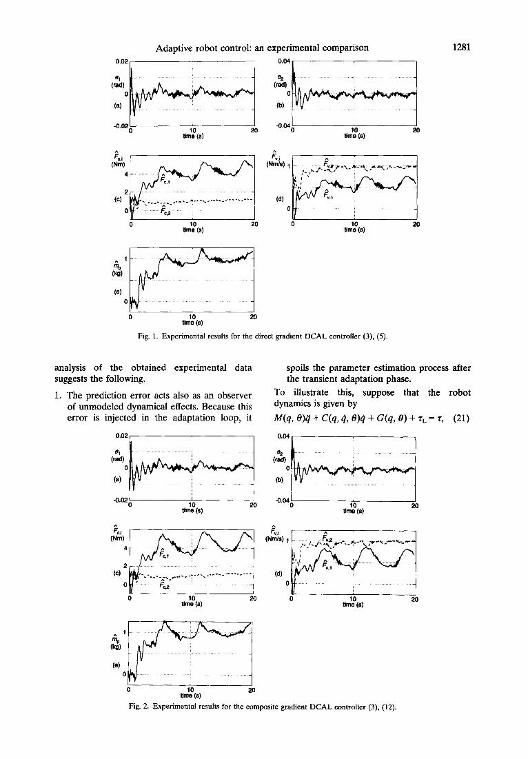
4.1.1. Direct gradient adaptation. The direct estimator (5) contains two design parameters: the diagonal adaptation gain matrix I0 > 0 and the sliding gain A,, >O. These gains were determined empirically by experimentation on the real setup, in such a way that sufficiently fast but stable adaptation was obtained. This resulted in I0 = diag (5,100,100,10,25), and A0 = 3. Figure 1 shows the data obtained from this experiment. Note that the control performance improves after the transient phase: the controller effectively exploits its adaptation capabilities in order to enhance the tracking accuracy. In particular the payload-sensitive lower link profits from this. For this experiment we obtained J1 = 9.34 X 10e6 and J2 = 2.87 X 10W5.

4. EXPERIMENTAL EVALUATION OF PARAMETER ESTIMATION METHODS

Extensive experiments were carried out with the DCAL controller (3) in combination with the following parameter estimation methods:

l direct gradient adaptation (5);

l composite gradient adaptation (12);

The erratic behavior of pc,l(t) and f?&(t) suggests that the friction in the upper joint cannot be described by viscous and Coulomb effects only. Indeed, attached to the upper joint are two cylinders that, though switched off during the experiments, can be used to compensate for the gravitation on the upper link. However, these cylinders introduce a difficult-to- model asymmetric and position-dependent fric- tion disturbance in the upper joint. As can be seen from Figs l(c, d) this friction disturbance becomes more important for increasing negative amplitudes of the upper link. Relative to this, the friction in the lower motor drive appears to be truly viscous and Coulomb; see ficc,2(t) and &(t) in Figs l(c, d).

l composite unnormalized least-squares adapta- tion (13), (14).

The results of these experiments are described in Sections 4.1 and 4.2. The former discusses some selective data that highlight the characteristics of the various parameter estimators. Section 4.2 presents performance figures of the estimation methods under a large variation of operational conditions.

4.1. Features of the parameter estimation methods

The data shown in the figures were obtained with the following reference trajectory:

qdl(f) = -Ai sin (@It),

q&t) = AZ sin (WZt),

(I9a)

(19b)

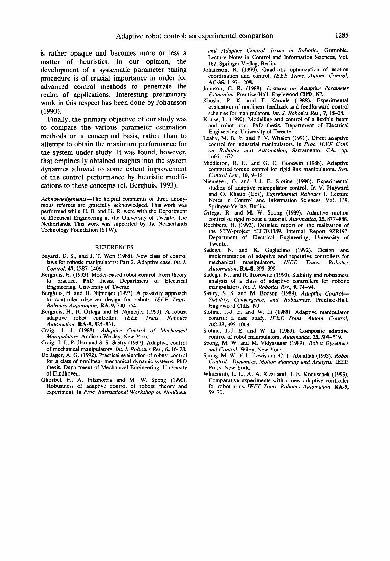
4.1.2. Composite gradient adaptation. During some preliminary experiments, it was observed that the composite gradient adaptation law is rather sensitive to velocity measurement noise. Such noise introduces offsets in the parameter estimates, which ensue from the filtering actions in the prediction error part. Consequently, the control performance decreased dramatically in comparison with the direct gradient method. Hence the noise level in the filtered prediction error cf has to be diminished, which can be achieved in two ways. First, the bandwidth o of the filter in the prediction error generator can be decreased. Second, the weighing matrix R can be selected such to reduce the influence of noisy components in cf. Suitable choices for w and R were found to be

w = 1, R = diag (2 X 10p3, 10e4). (20)

where Al = 0.34 rad, A2 = 0.62 rad, w1 = To justify the choice of R, recall that, owing to 0.3~ rad SK’ and w2 = 0.7~ rad s-‘. This trajec- the differences in PD gains, the noise on the tory is chosen because it generates sufficient control torque r1 is larger than the noise on ~2. nonlinear dynamic coupling between the robot As a consequence, the same is true for &fl links, while preventing the actuators from relative to cf2, which is reflected in R. The

saturating. resulting data are given in Fig. 2. A thorough

Adaptive robot control: an experimental comparison 1281

(1, 0,

(a) _

(d)

0 tirl-E(a) 20

Fig. 1. Experimental results for the direct gradient DCAL controller (3), (5).

analysis of the obtained experimental data suggests the following.

1. The prediction error acts also as an observer of unmodeled dynamical effects. Because this error is injected in the adaptation loop, it

2

(c)

v 0 ’

“_-‘_._x,_“...__ *_-., _._-._-..-_^-.

F c2 1

spoils the parameter estimation process after the transient adaptation phase.

To illustrate this, suppose that the robot dynamics is given by

Mq, @ii + C(q, 4, +j + G(q, 6) + r, = r, (21)

-0.04 1 I 0

timleo 20

0 timleo 20

Fig. 2. Experimental results for the composite gradient DCAL controller (3), (12).

1282 H. Berghuis ef al.

where rL is a vector of disturbances. According to (7) a prediction ‘2 of r is given by

Z = M(q, b)cj + C(q, 4, &j + G(q, 8). (22)

Then the prediction error equals

&=+-_=Y(q,~,~,~)8-zL. (23)

This shows that, besides the parameter error 8, unmodeled disturbances r, are also reflected in E and cf. As indicated by (23), these disturbances become increasingly dominant in the prediction error after the transient adaptation phase. The disturbance-observer nature of the prediction error method is illustrated in Fig. 3, which shows the prediction error cfl on the control torque of the upper drive. In this figure the asymmetric and position-dependent friction disturbance in the upper drive (cf. Section 4.1.1 and Figs lc, d) can clearly be seen.

The ‘polluted’ cfl is injected in the adaptation loop. As a consequence, the adaptation process not only compensates for the uncertainty in the parameters, but also tries to reject the friction disturbance. This may improve the performance. In the underlying case, Efl influences &(t), p,,,(t) and tip(t). As can be seen from Figs 2(c,d), pc,r(t) and &(t) in particular are employed to compensate for the unmodeled friction effect in the upper link, compare with Figs l(c, d). This yields an increase in control performance of the upper link, from J, = 9.34 X 1O-6 for direct adaptation to J1 = 9.10 X

10e6 here. Unfortunately, this improvement is not without peril: cfl also affects h,(j), which causes a slight deterioration of the tracking accuracy of the payload-sensitive lower link: J2 = 2.92 X 10d5 compared with J2 = 2.87 X 10e5 for direct adaptation. In spite of the potential performance benefits, the aforementioned use of the prediction error concept for disturbance rejection should not be advocated, because of its high sensitivity to the kind of disturbances, and its necessity for careful parameter tuning.

2. Under ideal circumstances, the composite

5

(tz, 0

-5

0 10 20 time (s)

Fig. 3. Prediction error of the upper link.

adaptation method yields faster zero conver- gence of the prediction error in comparison with the direct method.

In contrast to the upper link, the lower link is almost free of unmodeled effects. This is illustrated in Fig. 4, which shows the absolute value of the filtered prediction error of the lower link for both the direct and the composite method. As can be seen, the composite method drives the prediction error faster to zero than the direct method. Hence, under ideal circum- stances, the prediction error concept may enhance the performance.

In our opinion the merit of the prediction error concept is that it provides valuable additional insight into the system dynamics that may be used to improve the dynamical model employed in the control loop. As an example, the information contained in Fig. 3 could be used to develop a phenomenological description of the asymmetric friction disturbance that can be included in the control model.

4.1.3. Composite least-squares adaptation. The gradient-based adaptation methods are relatively slow, which can be seen from Figs 1 and 2: the transient period in the adaptation takes ap- proximately 5 s. Faster convergence can be obtained by employing the unnormalized least- squares-based composite method (13), (14). In the following experiment this method was examined with I(O) set at I(O) = diag (100,100,100,10,25). Compared with IO, this gain is larger in its first element, which represents the adaptation gain for n$,(t). To justify this choice, note that the system dynamics is most sensitive to uncertainty in m,; hence it is desired to obtain a fast convergent mass estimate. But since such a large adaptation gain makes h,(t) rather sensitive to noise, Rz2 was also reselected as R 22 = 0.1, which causes I’,,(t) to increase at a significantly faster rate. Figure 5 shows the experimental results obtained with (3,13,14).

Figure 5 demonstrates the powerful conver- gence properties of least-squares algorithms relative to gradient methods (see Figs le,2e). The corresponding indices are equal to 5, = 9.22 x 10m6 and J2 = 2.67 X 10-5. In particular, the tracking of the load-sensitive lower link improves owing to the fast convergent mass estimate. Another reason for this improvement is that the adaptive loop is nearly turned off after a while because I(t) has a tendency to vanish for the unnormalized least-squares method (14). This is illustrated in Fig. 6 for the payload mass adaptation gain I,,(t). Consequently, after the transient period, &Jr) is no longer negatively

Adaptive robot control: an experimental comparison

I%1 I%1 (NM (NM

(a) (W

0 0

tim5e (s) 10

Fig. 4. Prediction error of the lower link for direct (a) and composite (b) adaptation.

1283

affected by the unmodeled friction disturbance

m Efl (cf. Section 4.1.2). On the contrary, the disconnection of the adaptive loop also prevents pc,r(t) and fiV,I(t) from compensating for this friction disturbance, which explains why .I1 of the least-squares composite method is slightly worse than Jr of the gradient composite method.

4.2. Comparative experiments for various reference trajectories

To allow for general conclusions, an ensemble of runs were performed under different operating conditions. For this purpose, five sinusoidal test trajectories were considered, which span a wide range of the operational space of the robot. For brevity, only the performance indices of the different controllers are shown in Fig. 7. As before, these indices represent the means of five runs. The amplitudes A,, A2 and frequencies ol, w2 refer back to (19). For convenience, the data in Fig. 7 are normalized

with respect to performance index of the direct gradient method. The results shown in Fig. 7 reveal the following.

Composite gradient adaptation generally provides a small improvement in the upper link relative to direct gradient adaptation, because it (mis)uses the adaptation loop to compensate for the uncertain friction distur- bance in the upper link. As far as the lower link is concerned, the first method is overall worse owing to the negative influence of the unmodeled disturbance on the payload mass estimate (see Section 4.1.2).

On average, the least-squares composite adaptation method is more attractive than the gradient direct adaptation method, although the improvement is relatively small.

Because sampling aspects are an important issue, we implement a counter determining the period needed to compute the different control

0.04, I

(I,

(a)

, I 0

timT(e) 20

-0.04; I

tin?(s) 20

60

Fig. 5. Experimental results for the composite least-squares DCAL controller (3), (13), (14).

H. Berghuis et al.

1 3

time (8)

Fig. 6. Monotonically decreasing adaptation gain for the payload mass.

algorithms. For the gradient methods this period was evaluated as 410 ps, whereas the least- squares method required 600 ps. This indicates the significant increase in computational burden of the least-squares method. It was also observed that the sampling rate of the model-based compensation part including the adaptive loop could be decreased to 100 Hz without any measurable performance degradation.

5. CONCLUSIONS One of the main issues to be resolved is the

An experimental comparison between development of suitable design guidelines that

different parameter estimation methods for facilitate the gain tuning process. Especially for

adaptive robot control has been given. Our data large sets of adjustable parameters, this process

indicate on the one hand that in practice the usefulness of the prediction error concept for enhanced control performance is decreased owing to the presence of unmodeled effects. On the other hand, because torque disturbances such as uncertain friction effects are directly reflected in the prediction error, this concept gives valuable additional insight into the system dynamics that may be employed to improve the control model. Concerning least-squares adapta- tion, we observe that it increases the parameter convergence rate, which on average yields some improvement in control quality. However, this marginal improvement is attained at the cost of an increase in computational complexity. In addition, the least-squares method is rather sensitive to noise owing to the filtering actions in the prediction error generation part. On the basis of these observations, we (cautiously) conclude that in robotic applications the gradient-based direct method is to be preferred for parameter adaptation.

Jl J2

1.3 _ .................................. 1.3 ....................................

1.2 _ .................................. 1.2 ....................................

1.1 _ .................................. 1.1 ...................................

1.0 1.0

0.9 0.9

0.6 0.6

0.7 0.7

0.6 0.6

AkO.26 Al=034 A1=0.40 Ab0.26 A1=0.34 Ab0.40 A2==0.41 A2=0.62 A2=0.63 A2=0.41 AhO. A2=0.63

Constant frequency (wl=O.3x 02=0.7x)

Jl

1.3 _ .......................... ........

1.2.. ......................... .........

,,, _ ..................................

J2

1.0 1.0

0.9 0.9

0.6 0.6

0.7 0.7

0.6 0.6

ol=Oo.2n 01=0.3x 01=0.4n oko.2x okO.3n 01=0).4x

d?=Osn c&0.7x w2=0.9n o2=Osn 02=0.7x 02=0.9x

Constant amplitude (Al =0.34 A2~0.62)

Fig. 7. Mean-square tracking errors for different test trajectories.

Adaptive robot control: an experimental comparison 1285

is rather opaque and becomes more or less a matter of heuristics. In our opinion, the development of a systematic parameter tuning procedure is of crucial importance in order for advanced control methods to penetrate the realm of applications. Interesting preliminary work in this respect has been done by Johansson

(199% Finally, the primary objective of our study was

to compare the various parameter estimation methods on a conceptual basis, rather than to attempt to obtain the maximum performance for the system under study. It was found, however, that empirically obtained insights into the system dynamics allowed to some extent improvement of the control performance by heuristic modifi- cations to these concepts (cf. Berghuis, 1993).

Acknowledgemenrs-The helpful comments of three anony- mous referees are gratefully acknowledged. This work was performed while H. B. and H. R. were with the Department of Electrical Engineering at the University of Twente, The Netherlands. This work was supported by the Netherlands Technology Foundation (STW).

REFERENCES

Bayard, D. S., and J. T. Wen (1988). New class of control laws for robotic manipulators: Part 2. Adaptive case. Inr. J. Control, 47, 1387-1406.

Berghuis, H. (1993). Model-based robot control: from theory to practice. PhD thesis. Department of Electrical Engineering, University of Twente.

Berghuis, H. and H. Nijmeijer (1993). A passivity approach to controller-observer design for robots. IEEE Trans. Robotics Automation, RA-9, 740-754.

Berghuis, H., R. Ortega and H. Nijmeijer (1993). A robust adaptive robot controller. IEEE Trans. Robotics Automation, RA-9,825-831.

Craig, J. J. (1988). Adaptive Control of Mechanical Manipulators. Addison-Wesley, New York.

Craig, J. J., P. Hsu and S. S. Sastry (1987). Adaptive control of mechanical manipulators. Int. 1. Robotics Res., 6, 16-28.

De Jager, A. G. (1992). Practical evaluation of robust control for a class of nonlinear mechanical dynamic systems. PhD thesis, Department of Mechanical Engineering, University of Eindhoven.

Ghorbel, F., A. Fitzmorris and M. W. Spong (1990). Robustness of adaptive control of robots: theory and experiment. In Proc. International Workshop on Nonlinear

and Adaptive Control: Issues in Robotics, Grenoble. Lecture Notes in Control and Information Sciences, Vol. 162, Springer-Verlag, Berlin.

Johansson, R. (1990). Quadratic optimization of motion coordination and control. IEEE Trans. Autom. Control, AC-35,1197-1208.

Johnson, C. R. (1988). Lectures on Adaptive Parameter Estimation. Prentice-Hall, EngIewood Cliffs, NJ.

Khosla. P. K. and T. Kanade (1988). Exwrimental evaluation of nonlinear feedback and feedforward control schemes for manipulators. Int. J. Robotics Res., 7, 18-28.

Kruise, L. (1990). Modelling and control of a flexible beam and robot arm. PhD thesis, Department of Electrical Engineering, University of Twente.

Leahy, M. B. Jr, and P. V. Whalen (1991). Direct adaptive control for industrial manipulators. In Proc. IEEE Conf. on Robotics and Automation, Sacramento, CA, pp. 1666-1672.

Middleton, R. H. and G. C. Goodwin (1988). Adaptive computed torque control for rigid link manipulators. Syst. Control Lett., 10, 9-16.

Niemeyer, G. and J.-J. E. Slotine (1990). Experimental studies of adaptive manipulator control. In V. Hayward and 0. Khatib (Eds), Experimental Robotics I. Lecture Notes in Control and Information Sciences, Vol. 139, Springer-Verlag, Berlin.

Ortega, R. and M. W. Spong (1989). Adaptive motion control of rigid robots: a tutorial. Automatica. 25.877-888.

Roebbers, H.11992). Detailed report on the reahzation of the STW-project tEL70.1389. Internal Report 92R197, Department of Electrical Engineering, University of Twente.

Sadegh, N. and K. Guglielmo (1992). Design and implementation of adaptive and repetitive controllers for mechanical manipulators. IEEE Trans. Robotics Automation, RA-8, 395-399.

Sadegh, N., and R. Horowitz (1990). Stability and robustness analysis of a class of adaptive controllers for robotic manipulators. Int. J. Robotics Res., 9, 74-94.

Sastry, S. S. and M. Bodson (1989). Adaptive Control- Stability, Convergence, and Robustness. Prentice-Hall, Englewood Cliffs, NJ.

Slotine, J.-J. E. and W. Li (1988). Adaptive manipulator control: a case study. IEEE Trans. Autom. Control, AC-33,995-1003.

Slotine, J.-J. E. and W. Li (1989). Composite adaptive control of robot manipulators. Automatica, 25,509-519.

Spong, M. W. and M. Vidyasagar (1989). Robot Dynamics and Control. Wiley, New York.

Spong, M. W., F. L. Lewis and C. T. Abdallah (1993). Robot Control-Dynamics, Motion Planning and Analysis. IEEE Press, New York.

Whitcomb, L. L., A. A. Rizzi and D. E. Koditschek (1993). Comparative experiments with a new adaptive controller for robot arms. IEEE Trans. Robotics Automation, RA-9, 59-70.