Experimental characterization of towers in cable-supported ...

Experimental Characterization of Towers in Cable-Supported Bridges

by Ambient Vibration Testing

Volume 1

A Thesis

Submitted to the Faculty

of

Drexel University

by

Kirk Alexander Grimmelsman

in partial fulfillment of the

requirements for the degree

of

Doctor of Philosophy

December 2006

ii DEDICATIONS

To my parents.

iii ACKNOWLEDGEMENTS

I would like to acknowledge the guidance and support provided by my advisor, Dr. A.

Emin Aktan. I sincerely appreciate Dr. Aktan’s excellent mentorship and encouragement

throughout my graduate studies. I would also like to thank the members of my

dissertation committee, Drs. J. Awerbuch, A. Lau, F. Moon, and T. Tan for their interest,

participation, and advice. The support provided by the Mechanical Engineering and

Mechanics Department at Drexel University throughout my studies is gratefully

acknowledged. I would also like to thank the MEM Department Head, Dr. Mun Choi, for

providing financial support and encouragement as I completed my research.

I would also like to thank Dr. Bart Peeters and LMS International for providing the

TestLab software package which was used extensively in this study. I would also like to

thank the New York City Department of Transportation and Dr. Arzoumanidis from

Parsons Transportation Group for the opportunity to test the Brooklyn Bridge. My

position at Drexel University has been partially supported by research funding from the

Federal Highway Administration, and I would like to acknowledge this support and the

encouragement given by Drs. S. Chase, H. Ghasemi, and F. Jalinoos.

I would like to gratefully acknowledge the help and support provided by my friends and

colleagues. In particular, I would like to acknowledge John Prader, Qin Pan, and Korhan

Ciloglu for their enthusiastic assistance with this research. I also wish to thank my friend

and former colleague, Dr. F.N. Catbas at the University of Central Florida for his helpful

advice and support. Finally, I would like to thank my family for their patience, love and

endless moral support.

iv TABLE OF CONTENTS

LIST OF TABLES............................................................................................................. ix

LIST OF FIGURES ........................................................................................................... xi

ABSTRACT...................................................................................................................... xx

CHAPTER 1 : INTRODUCTION...................................................................................... 1

1.1 Background............................................................................................................. 1

1.2 Motivation............................................................................................................... 5

1.3 Objectives and Scope.............................................................................................. 9

1.4 Thesis Structure .................................................................................................... 15

CHAPTER 2 : LITERATURE REVIEW......................................................................... 18

2.1 Introduction........................................................................................................... 18

2.2 Examples of Previously Characterized Towers .................................................... 20

2.2.1 Characterization of the Towers from Two Suspension Bridges ............... 20

2.2.2 Characterization of the Towers in the Golden Gate Bridge...................... 21

2.2.3 Characterization of the Towers in the Humber Bridge............................. 28

2.2.4 Characterization of the Towers in the Bosporus Suspension Bridge........ 30

2.2.5 Characterization of the Towers in the Second Bosporus Suspension Bridge................................................................................................ 32

2.2.6 Characterization of the Towers in the Tsing Ma Suspension Bridge ....... 34

2.2.7 Characterization of the Towers in a Long-Span Cable-Stayed Bridge..... 38

2.3 Summary ............................................................................................................... 40

CHAPTER 3 : AMBIENT VIBRATION TESTING OVERVIEW................................. 47

3.1 Introduction........................................................................................................... 47

3.2 Basic Assumptions................................................................................................ 48

v 3.3 Experimental Considerations ................................................................................ 49

3.4 Identification of Modal Properties ........................................................................ 51

3.4.1 Frequency Domain Identification Methods .............................................. 51

3.4.2 Time Domain Modal Identification Methods ........................................... 58

CHAPTER 4 : AMBIENT VIBRATION TEST OF THE BROOKLYN BRIDGE TOWERS .......................................................................................................................... 63

4.1 Introduction........................................................................................................... 63

4.2 Description of the Brooklyn Bridge...................................................................... 66

4.3 Previous Dynamic Characterization of the Spans................................................. 68

4.3.1 Summary Findings from the Vibration Tests of the Spans....................... 69

4.4 Test Description .................................................................................................... 70

4.4.1 Proposed Test Procedure........................................................................... 70

4.4.2 Instrumentation Scheme............................................................................ 73

4.4.3 Sensors and Data Acquisition ................................................................... 78

4.4.4 Test Execution .......................................................................................... 84

4.5 Data Processing and Analysis............................................................................... 86

4.5.1 Data Pre-Processing.................................................................................. 86

4.5.2 Modal Parameter Identification by Peak-Picking Method........................ 94

4.6 Results................................................................................................................... 98

4.6.1 Amplitudes of Acceleration Signals ......................................................... 99

4.6.2 Spectral Content of Acceleration Signals ............................................... 101

4.6.3 Time Variation of Spectral Content........................................................ 106

4.6.4 Natural Frequencies and Mode Shapes................................................... 116

4.7 Discussion........................................................................................................... 125

4.7.1 Longitudinal Modes ................................................................................ 126

4.7.2 Torsional Modes ..................................................................................... 129

vi 4.7.3 Lateral Modes ......................................................................................... 130

4.7.4 Summary Modes ..................................................................................... 131

CHAPTER 5 : ANALYTICAL STUDY OF THE BROOKLYN BRIDGE .................. 134

5.1 Introduction......................................................................................................... 134

5.2 Objectives and Scope.......................................................................................... 137

5.3 Structural Characteristics of the Brooklyn Bridge.............................................. 140

5.3.1 Masonry Towers ..................................................................................... 141

5.3.2 Suspended Structure................................................................................ 146

5.3.3 Main Cables ............................................................................................ 147

5.4 Idealized Analytical Model of the Brooklyn Bridge........................................... 148

5.4.1 Towers..................................................................................................... 148

5.4.2 Stiffening Trusses ................................................................................... 150

5.4.3 Main Cables ............................................................................................ 150

5.4.4 Stay Cables.............................................................................................. 151

5.5 Results................................................................................................................. 152

5.6 Discussion........................................................................................................... 164

CHAPTER 6 : MODAL IDENTIFICATION OF A CANTILEVER BEAM................ 169

6.1 Introduction......................................................................................................... 169

6.2 Scope................................................................................................................... 174

6.3 Description of the Test Specimen ....................................................................... 176

6.3.1 Theoretical Dynamic Properties of the Cantilever Beam ....................... 178

6.4 Ambient Dynamic Excitation Characteristics for Cable-Supported Bridges ..... 183

6.5 Dynamic Excitation Cases .................................................................................. 189

6.6 Experimental Setup............................................................................................. 194

6.7 Data Analysis ...................................................................................................... 199

vii 6.7.1 Data Pre-Processing................................................................................ 201

6.7.2 Identification of Modal Parameters ........................................................ 207

6.8 Results................................................................................................................. 221

6.8.1 Spectral Densities for Excitation Cases .................................................. 221

6.8.2 Peak Selection Criteria and Mode Indicator Functions .......................... 223

6.8.3 Natural Frequencies and Mode Shapes................................................... 227

6.9 Discussion........................................................................................................... 274

6.9.1 Identification Methods ............................................................................ 275

CHAPTER 7 : RIGOROUS MODAL IDENTIFICATION OF THE BROOKLYN BRIDGE TOWERS ........................................................................................................ 283

7.1 Introduction......................................................................................................... 283

7.2 Scope................................................................................................................... 286

7.3 Data Processing................................................................................................... 289

7.3.1 Peak-Picking (PP) ................................................................................... 289

7.3.2 Stochastic Subspace Identification (SSI) ................................................ 297

7.3.3 Polyreference Time Domain (PTD)........................................................ 297

7.3.4 Complex Mode Indicator Function (CMIF) ........................................... 300

7.4 Results................................................................................................................. 301

7.4.1 Peak Selection Criteria and Mode Indicator Functions for PP ............... 301

7.4.2 Tower Longitudinal Natural Frequencies and Mode Shapes.................. 303

7.4.3 Tower Torsional Natural Frequencies and Mode Shapes ....................... 347

7.4.4 Tower Lateral Natural Frequencies and Mode Shapes ........................... 368

7.5 Discussion........................................................................................................... 397

7.5.1 Effectiveness of the Automated Peak Picking Procedure....................... 397

7.5.2 Identification of the Tower Modes from Peak Picking Results.............. 399

7.5.3 Performance of the Advanced Modal Identification Methods................ 407

viii CHAPTER 8 : CONCLUSIONS AND FUTURE WORK............................................. 411

8.1 Introduction......................................................................................................... 411

8.2 Fundamental Dynamic Behavior for a Tower in a Cable-Supported Bridge...... 414

8.3 Character of the Ambient Dynamic Excitation................................................... 418

8.4 Effectiveness of Different Modal Identification Methods .................................. 421

8.5 Experiment Design.............................................................................................. 432

8.6 Future Work ........................................................................................................ 434

LIST OF REFERENCES................................................................................................ 436

VITA............................................................................................................................... 441

ix LIST OF TABLES

Table 4.1. Performance characteristics of the piezoelectric and capacitive

accelerometers................................................................................................. 81

Table 4.2. Characteristics of spectral peaks identified from SPSD function for tower longitudinal response .................................................................................... 119

Table 4.3. Characteristics of spectral peaks identified from ANPSD function for tower torsional response.......................................................................................... 119

Table 4.4. Characteristics of spectral peaks identified from ANPSD function for tower lateral response.............................................................................................. 120

Table 4.5. Brooklyn Tower modes identified by ambient vibration testing ................... 132

Table 5.1. Brooklyn Tower modes for different model cases......................................... 153

Table 6.1. Mechanical and material properties of the cantilever beam .......................... 177

Table 6.2. Theoretical natural frequencies and mode shape coordinates for the cantilever beam.............................................................................................................. 182

Table 6.3. Number of spectral peaks identified by selection criterion and MIF ............ 226

Table 6.4. Number of spectral peaks identified for each MIF with minimum threshold criterion ......................................................................................................... 226

Table 6.5. Spectral peaks by PP for BB400 excitation case ........................................... 228

Table 6.6. Characteristics of spectral peaks identified for BB400 excitation case......... 233

Table 6.7. Final Identified Frequencies and MAC Values: Random Finger Taps Excitation Case ............................................................................................. 270

Table 6.8. Experimental frequencies and mode shapes from multiple reference impact test ..................................................................................................... 273

Table 6.9. Final Identified Frequencies and MAC Values: BB400 & NB200 Excitation Cases ............................................................................................................. 280

Table 6.10. Final Identified Frequencies and MAC Values: NB50 & NB10 Excitation Cases ............................................................................................................. 281

Table 6.11. Final Identified Frequencies and MAC Values: H1 Excitation Case .......... 282

Table 7.1. Number and Distribution Bridge Responses Evaluated ................................ 294

x Table 7.2. Number of spectral peaks identified by PP for each selection criteria

and MIF......................................................................................................... 303

Table 7.3. Number of Spectral Peaks Identified by PP Selection Criteria and MIF with Thresholds..................................................................................................... 303

Table 7.4. Spectral peaks identified by PP from SPSD function for Brooklyn Tower longitudinal vibrations .................................................................................. 327

Table 7.5. Comparison of %SSCOH values - tower longitudinal references and all other bridge responses............................................................................................ 330

Table 7.6. Comparison of tower longitudinal spectral peaks with span identification results ............................................................................................................ 331

Table 7.7. Summary evaluation results for identifying pure longitudinal tower modes. 332

Table 7.8. Spectral peaks identified by PP from ANPSD function for Brooklyn Tower torsional vibration ......................................................................................... 350

Table 7.9. Comparison of %SSCOH values - tower torsional references and all other bridge responses............................................................................................ 351

Table 7.10. Comparison of tower torsional spectral peaks with span identification results ............................................................................................................ 351

Table 7.11. Summary evaluation results for identifying pure torsional tower modes.... 354

Table 7.12. Spectral peaks identified by PP from ANPSD function for Brooklyn Tower lateral vibrations............................................................................................ 373

Table 7.13. Comparison of %SSCOH values - tower lateral references and all other bridge responses............................................................................................ 373

Table 7.14. Comparison of tower lateral spectral peaks with span identification results ............................................................................................................ 374

Table 7.15. Summary evaluation results for identifying pure lateral tower modes........ 383

xi LIST OF FIGURES

Figure 1.1. Classification of available short-term experiments for objective

characterization of constructed systems............................................................ 4

Figure 1.2. Classification of available long-term experiments for objective characterization of constructed systems............................................................ 4

Figure 1.3. Different stages in the structural identification framework.............................. 5

Figure 1.4. Flowchart illustrating the experimental and analytical components of the research ........................................................................................................... 13

Figure 1.5. Flowchart summarizing the analytical component of the research ................ 13

Figure 1.6. Overview of the experimental component for the cantilever ......................... 14

Figure 1.7. Overview of the experimental component for the full-scale tower vibration measurements.................................................................................................. 14

Figure 4.1. Overview of the Brooklyn Bridge .................................................................. 67

Figure 4.2. Overview of the Brooklyn Bridge Towers ..................................................... 67

Figure 4.3. Pedestrians crossing the Brooklyn Bridge during electrical blackout............ 69

Figure 4.4. Eccentric mass shaker from Utah State University ........................................ 71

Figure 4.5. First three tower modes from preliminary FE models.................................... 72

Figure 4.6. Measurement levels on the Brooklyn and Manhattan Towers ....................... 75

Figure 4.7. Accelerometer layout at the lower measurement levels on the towers .......... 76

Figure 4.8. Accelerometer layout at the upper measurement levels on the towers .......... 76

Figure 4.9. Installation of accelerometers on the Brooklyn Tower .................................. 77

Figure 4.10. Locations of the measurement stations for the spans ................................... 77

Figure 4.11. Arrangement of the accelerometers on the stiffening trusses....................... 78

Figure 4.12. Piezoelectric (Model 393C) and capacitive type (Model 3701) accelerometers................................................................................................. 81

Figure 4.13. Ultrasonic anemometer on top of the Brooklyn Tower................................ 82

xii Figure 4.14. Data acquisition system components............................................................ 85

Figure 4.15. Data acquisition cabinet on inspection walkway.......................................... 85

Figure 4.16. Large and small spurious spikes in the raw time domain acceleration records ........................................................................................ 91

Figure 4.17. Removal of spurious responses from acceleration record............................ 91

Figure 4.18. Effect of different combination methods for channel with large spurious peaks........................................................................................ 92

Figure 4.19. Effect of different combination methods for channel with small spurious peaks ....................................................................................... 92

Figure 4.20. Effect of different combination methods for channel with no spurious peaks............................................................................................ 93

Figure 4.21. Acceleration amplitudes for vertical span and longitudinal tower vibrations ............................................................................................ 100

Figure 4.22. Acceleration amplitudes for lateral span and tower vibrations .................. 101

Figure 4.23. Autospectral densities for longitudinal and torsional vibrations of the towers ...................................................................................................... 103

Figure 4.24. Autospectral densities for lateral (transverse) vibrations of the towers ..... 104

Figure 4.25. Autospectral densities for the vertical and torsional vibrations of the main and side spans ............................................................................................... 105

Figure 4.26. Autospectral densities for the lateral vibrations of the main and side spans................................................................................. 106

Figure 4.27. Variation of spectral content with time for tower longitudinal vibrations . 109

Figure 4.28. Variation of spectral content with time for tower torsional vibrations ...... 110

Figure 4.29. Variation of spectral content with time for tower lateral vibrations .......... 111

Figure 4.30. Time domain responses corresponding to unusual spectral content .......... 112

Figure 4.31. Variation of spectral content with time for vertical vibrations of the spans ..................................................................... 113

Figure 4.32. Variation of spectral content with time for torsional vibrations of the spans .................................................................................. 114

Figure 4.33. Variation of spectral content with time for lateral vibrations of the spans 115

xiii Figure 4.34. Operating deflection shapes at spectral peaks for

tower longitudinal response .......................................................................... 120

Figure 4.35. Operating deflection shapes at spectral peaks for tower torsional response ............................................................................... 121

Figure 4.36. Operating deflection shapes at spectral peaks for tower lateral response (north tower column) .................................................................................... 122

Figure 4.37. Operating deflection shapes at spectral peaks for tower lateral response (middle tower column).................................................................................. 123

Figure 4.38. Operating deflection shapes at spectral peaks for tower lateral response (south tower column) .................................................................................... 124

Figure 4.39. Eccentricity of transverse accelerometers for torsional vibrations............. 133

Figure 5.1. Elevation view of the Brooklyn Bridge........................................................ 141

Figure 5.2. Front and side elevation views of the Brooklyn Tower ............................... 142

Figure 5.3. Brooklyn Tower dimensions at Section A-A and Section B-B.................... 143

Figure 5.4. Brooklyn Tower dimensions at Section C-C and Section D-D.................... 144

Figure 5.5. Brooklyn Tower dimensions at Section E-E and Section F-F...................... 145

Figure 5.6. Representation of towers in analytical model .............................................. 149

Figure 5.7. Representation of different bridge components in the idealized model ....... 154

Figure 5.8. Principal bridge components included in different analytical model cases .............................................................................................................. 154

Figure 5.9. First six modes of the Brooklyn Tower from the free-standing towers analysis case.................................................................................................. 157

Figure 5.10. First longitudinal, lateral and torsional modes of the Brooklyn Tower ..... 159

Figure 5.11. Second longitudinal, lateral and torsional modes of the Brooklyn Tower . 160

Figure 5.12. 1st and 2nd unit normalized longitudinal mode shapes for different model cases .............................................................................................................. 161

Figure 5.13. 1st and 2nd unit normalized lateral mode shapes for different model cases .............................................................................................................. 162

Figure 5.14. 1st and 2nd unit normalized torsional mode shapes for different model cases .............................................................................................................. 163

xiv Figure 5.15. Longitudinal modal displacements of Brooklyn Tower at discrete span

and tower modes ........................................................................................... 163

Figure 6.1. Cantilever beam specimen in the laboratory ................................................ 176

Figure 6.2. Clamped support condition for the cantilever beam..................................... 177

Figure 6.3. Theoretical unit normalized mode shapes for the cantilever beam .............. 182

Figure 6.4. Classification of ambient dynamic excitation for in-service bridges ........... 184

Figure 6.5. Spatial localization of transmitted ambient excitations................................ 187

Figure 6.6. Overview of dynamic excitation cases ......................................................... 195

Figure 6.7. Accelerometer layout for the cantilever beam specimen ............................. 197

Figure 6.8. Linear electrodynamic shaker....................................................................... 198

Figure 6.9. Eccentric mass shaker................................................................................... 198

Figure 6.10. Shakers installed on rear projection of cantilever beam............................. 199

Figure 6.11. Flowchart for PP implementation............................................................... 208

Figure 6.12. Criteria for automatic identification of spectral peaks in a MIF ................ 214

Figure 6.13. Application of minimum threshold for automated identification of peaks ......................................................................................................... 215

Figure 6.14. Autospectral density plots for random excitation cases ............................. 222

Figure 6.15. Autospectral density plots for random excitation cases with superimposed harmonic excitation....................................................................................... 222

Figure 6.16. Autospectral density plot for H1 excitation case........................................ 223

Figure 6.17. Possible natural frequencies and mode shapes by PP (BB400 excitation case)................................................................................ 234

Figure 6.18. Possible natural frequencies and mode shapes by SSI (BB400 excitation case)................................................................................ 235

Figure 6.19. Possible natural frequencies and mode shapes by CMIF (BB400 excitation case)................................................................................ 236

Figure 6.20. Possible natural frequencies and mode shapes by PTD (BB400 excitation case)................................................................................ 237

xv Figure 6.21. Experimental natural frequencies and mode shapes by PP

(NB200 excitation case)................................................................................ 240

Figure 6.22. Possible natural frequencies and mode shapes by SSI (NB200 excitation case)................................................................................ 240

Figure 6.23. Possible natural frequencies and mode shapes by CMIF (NB200 excitation case)................................................................................ 241

Figure 6.24. Possible natural frequencies and mode shapes by PTD (NB200 excitation case)................................................................................ 242

Figure 6.25. Experimental natural frequencies and mode shapes by PP (NB50 excitation case).................................................................................. 245

Figure 6.26. Mode shapes at discrete frequency lines near the 5th Mode (NB50 Excitation Case) ................................................................................ 246

Figure 6.27. Single-reference mode shapes at identified peaks near the 5th Mode of the cantilever beam ............................................................................................. 247

Figure 6.28. Multiple-reference mode shapes at identified peaks near the 5th Mode of the cantilever beam ............................................................................................. 247

Figure 6.29. Experimental natural frequencies and mode shapes by SSI (NB50 excitation case).................................................................................. 248

Figure 6.30. Possible natural frequencies and mode shapes by CMIF (NB50 excitation case).................................................................................. 249

Figure 6.31. Possible natural frequencies and mode shapes by PTD (NB50 excitation case).................................................................................. 250

Figure 6.32. Experimental natural frequencies and mode shapes by PP (NB10 excitation case).................................................................................. 252

Figure 6.33. Possible natural frequencies and mode shapes by SSI (NB10 excitation case).................................................................................. 252

Figure 6.34. Possible natural frequencies and mode shapes by CMIF (NB10 excitation case).................................................................................. 253

Figure 6.35. Possible natural frequencies and mode shapes by PTD (NB10 excitation case).................................................................................. 254

Figure 6.36. Identified natural frequencies and mode shapes by PP for BB400+H1 excitation case............................................................................................... 255

xvi Figure 6.37. Identified natural frequencies and mode shapes by PP for NB200+H1

excitation case............................................................................................... 256

Figure 6.38. Identified natural frequencies and mode shapes by PP for NB50+H1 excitation case............................................................................................... 256

Figure 6.39. Identified natural frequencies and mode shapes by PP for NB10+H1 excitation case............................................................................................... 257

Figure 6.40. Identified natural frequencies and mode shapes by SSI for BB400+H1 excitation case............................................................................................... 259

Figure 6.41. Identified natural frequencies and mode shapes by SSI for NB200+H1 excitation case............................................................................................... 259



Figure 6.44. Identified natural frequencies and mode shapes by CMIF for BB400+H1 excitation case............................................................................................... 261

Figure 6.45. Identified natural frequencies and mode shapes by CMIF for NB200+H1 excitation case............................................................................................... 261



Figure 6.48. Identified natural frequencies and mode shapes by PTD for BB400+H1 excitation case............................................................................................... 262

Figure 6.49. Identified natural frequencies and mode shapes by PTD for NB200+H1 excitation case............................................................................................... 262



Figure 6.52. Natural frequencies and mode shapes identified by PP for H1 excitation case............................................................................................... 266

xvii Figure 6.53. Mode shapes and phase factor values at spectral peak associated with

the H1 excitation ........................................................................................... 266

Figure 6.54. Mode shapes and phase factor values at the 1st Mode of cantilever beam ............................................................................................. 267

Figure 6.55. Natural frequencies and mode shapes by SSI for H1 excitation case ........ 267

Figure 6.56. Natural frequencies and mode shapes by CMIF for H1 excitation case .... 267

Figure 6.57. Natural frequencies and mode shapes by PTD for H1 excitation case....... 268

Figure 6.58. Natural frequencies and mode shapes by CMIF using correlation functions for random finger taps excitation case .......................................................... 270

Figure 6.59. Natural frequencies and mode shapes by CMIF using random decrement for random finger taps excitation case................................................................ 271

Figure 6.60. Natural frequencies and mode shapes by PTD using correlation functions for random finger taps excitation case................................................................ 271

Figure 6.61. Natural frequencies and mode shapes by PTD using random decrement for random finger taps excitation case................................................................ 272

Figure 7.1. Vibration responses at each level on Brooklyn Tower................................. 291

Figure 7.2. Unit normalized operating deflection shapes for longitudinal spectral peaks 1 – 16 .................................................................................................. 328

Figure 7.3. Unit normalized operating deflection shapes for longitudinal spectral peaks 17 – 25 ................................................................................................ 329

Figure 7.4. Raw phase factors between each output-reference pair at longitudinal spectral peak frequencies .............................................................................. 333

Figure 7.5. Raw phase factors between each output-reference pair at longitudinal spectral peak frequencies............................................................................................ 334

Figure 7.6. Brooklyn Tower longitudinal modes by SSI method ................................... 337

Figure 7.7. Brooklyn Tower longitudinal modes by SSI method ................................... 338

Figure 7.8. Brooklyn Tower longitudinal modes by PTD method from correlation functions........................................................................................................ 340

Figure 7.9. Brooklyn Tower longitudinal modes by PTD method from correlation functions........................................................................................................ 341

xviii Figure 7.10. Brooklyn Tower longitudinal modes by PTD from random decrement

functions........................................................................................................ 342

Figure 7.11. Brooklyn Tower longitudinal modes by CMIF from correlation functions........................................................................................................ 344

Figure 7.12. Brooklyn Tower longitudinal modes by CMIF from correlation functions345

Figure 7.13, Brooklyn Tower longitudinal modes by CMIF from random decrement functions........................................................................................................ 346

Figure 7.14. Unit normalized operating deflection shapes for torsional spectral peaks ............................................................................................................. 352

Figure 7.15. Raw phase factors between each output-reference pair at torsional spectral peak frequencies............................................................................................ 353

Figure 7.16. Tower torsional modes by SSI method ...................................................... 357

Figure 7.17. Tower torsional modes by SSI method ...................................................... 358

Figure 7.18. Brooklyn Tower torsional modes by PTD from correlation functions....... 360

Figure 7.19. Brooklyn Tower torsional modes by PTD from random decrement functions........................................................................................................ 361

Figure 7.20. Brooklyn Tower torsional modes by CMIF from correlation functions .... 364

Figure 7.21. Brooklyn Tower torsional modes by CMIF from correlation functions .... 365

Figure 7.22. Brooklyn Tower torsional modes by CMIF from random decrement functions........................................................................................................ 366

Figure 7.23. Brooklyn Tower torsional modes by CMIF from random decrement functions........................................................................................................ 367

Figure 7.24. Unit normalized operating deflection shapes for lateral spectral peaks (north tower column) ............................................................................................... 375

Figure 7.25. Unit normalized operating deflection shapes for lateral spectral peaks (north tower column) ............................................................................................... 376

Figure 7.26. Unit normalized operating deflection shapes for lateral spectral peaks (middle tower column).................................................................................. 377

Figure 7.27. Unit normalized operating deflection shapes for lateral spectral peaks (middle tower column).................................................................................. 378

xix Figure 7.28. Unit normalized operating deflection shapes for lateral spectral peaks (south

tower column) ............................................................................................... 379

Figure 7.29. Unit normalized operating deflection shapes for lateral spectral peaks (south tower column) ............................................................................................... 380

Figure 7.30. Raw phase factors between each output-reference pair at lateral spectral peak frequencies .................................................................................................... 381

Figure 7.31. Raw phase factors between each output-reference pair at lateral spectral peak frequencies .................................................................................................... 382

Figure 7.32. Tower lateral modes by SSI method (north, middle and south tower columns)........................................................................................................ 385

Figure 7.33. Tower lateral modes by SSI method (north, middle and south tower columns)........................................................................................................ 386

Figure 7.34. Lateral modes by PTD from correlation functions (north, middle and south tower columns).............................................................................................. 389

Figure 7.35. Lateral modes by PTD from random decrement functions (north, middle and south tower columns).................................................................................... 390

Figure 7.36. Lateral modes by CMIF from correlation functions (north, middle and south tower columns).............................................................................................. 393

Figure 7.37. Lateral modes by CMIF from correlation functions (north, middle and south tower columns).............................................................................................. 394

Figure 7.38. Lateral modes by CMIF from random decrement functions (north, middle and south tower columns) ............................................................................. 395

Figure 7.39. Lateral modes by CMIF from random decrement functions (north, middle and south tower columns) ............................................................................. 396

Figure 7.40. Brooklyn Tower modes from PP – 1st Longitudinal, 1st Lateral and 1st Torsional ....................................................................................................... 406

Figure 7.41. Brooklyn Tower modes from PP – 2nd Longitudinal, 2nd Lateral and 2nd Torsional ....................................................................................................... 407

xx ABSTRACT

Experimental Characterization of Towers in Cable-Supported Bridges by Ambient Vibration Testing

Kirk Alexander Grimmelsman A. Emin Aktan, Ph.D.

The objective of this thesis is to address several unresolved issues related to the

experimental characterization of the modal properties for the towers in cable-supported

bridges by the ambient vibration testing. A number of these unresolved issues were

identified during the application of this method to the towers in a landmark suspension

bridge. The research that was undertaken included both experimental and analytical

components. The experimental components consisted of: (1) characterizing the ambient

vibration environment for the masonry towers in the Brooklyn Bridge and evaluating the

limitations associated with the conventional approach for identifying the dynamic

properties by ambient vibration testing, (2) a laboratory investigation to compare and

evaluate the effectiveness of the most common and basic modal identification approach

for bridges, a multiple-reference channel extension of the basic approach and several

more sophisticated identification methods for the conditions of ambient dynamic

excitation that can occur for the towers in a cable-supported bridge, and (3) an

comparative evaluation of these same methods for characterizing the Brooklyn Bridge

towers. The focus of the analytical component was to characterize the fundamental

dynamic behavior for the towers using a idealized analytical model of a suspension

bridge.

This research indicated that the towers in a cable-supported bridge can have modes

which are distinct from the spans and vice-versa. Furthermore, it was possible to identify

the most likely dynamic properties of a tower by considering a spectrum of

xxi characteristics and parameter values associated with each identification result for the

complex vibration output spectra associated with the towers in cable-supported bridges;

however, the identified properties will not be free from uncertainty. The most consistent

and meaningful modal properties were identified by the peak picking identification

method using multiple reference locations. Visually comparing the consistency of the

operating mode shapes computed from multiple reference locations was also found to be

a very effective and intuitive approach for identifying spurious or poorly-excited modes

in the identification results.

1 CHAPTER 1: INTRODUCTION

1.1 Background

The constructed nature and the operational environment of civil infrastructure

systems often leads to significant uncertainty related to their in-service condition,

characteristics and performance. In most cases, this uncertainty is not a critical

consideration for assuring the safety of new or existing structures due to the level of

conservatism inherent in their designs. This conservatism is the result of numerous

simplifying assumptions and the use of empirical or probabilistic factors of safety in

conjunction with the design loads, the properties of the constituent materials, and the

computed capacities of the structural elements.

The uncertainty associated with constructed civil infrastructure systems does have a

significant influence on the cost and efficacy of engineering assessments and decisions

related to the operation, maintenance, and renewal of in-service structures. The degree to

which this uncertainty affects these assessments and decisions is a function of the data

available for use in managing these structures. Engineers and infrastructure owners have

traditionally relied on visual inspection techniques as one of the principal sources of this

data; however, this data is generally subjective in nature and has been shown to have

limitations with respect to accuracy and reliability (Moore, et al. 2001). Subjective data is

not well-suited to support reliable and cost effective management decisions, particularly

when coupled with conservative or simplified design assumptions.

The motivation to reduce the uncertainty associated with the in-service condition,

behavior, and performance of constructed systems is especially great for major bridges.

2 The US bridge inventory consists of far more short to medium span bridges than major

long span bridges; however, there are several important characteristics associated with

major bridges that justify additional measures to mitigate the uncertainty associated with

their in-service condition and behavior. Major bridges serve as critical or lifeline nodes of

the transportation network in most major metropolitan areas, and any disruptions or

limitations to their service will reverberate through the many other interconnected

infrastructure systems. Many major bridges are also considered as historic or landmark

structures, and there is a corresponding incentive to preserve them. Bridge owners desire

safe and reliable long term performance of their structures with minimal maintenance

costs. This objective is somewhat incompatible with the currently reactive and often

subjective approach generally used to manage and maintain such structures. Finally, the

societal and economic costs that result from a lack of performance for major bridge

structures, whether it is at the serviceability limit state or the safety limit state, can be

rather significant.

There are several possible ways to mitigate the uncertainty associated with major

bridges. One common approach is to employ more sophisticated and detailed analytical

models of a structure. Three dimensional FE models can offer a more accurate

representation of the various force resisting mechanisms by explicitly representing all of

the structural members. This will not completely mitigate the uncertainty since various

assumptions are still necessary to construct an analytical representation of a structure,

irrespective of the level of detail or sophistication utilized. Furthermore, an analytical

model can only simulate details and mechanisms that are known and may be reliably

3 conceptualized. Unknown or incompletely characterized details or mechanisms will

contribute uncertainty to the resulting analytical representation.

Another approach that may be used to reduce uncertainty is through objective

characterization of the structure or its subcomponents by field measurements and

experiments. The experimental characterization may be done at local levels using

nondestructive evaluation (NDE) methods, or at the global level using static or dynamic

field tests. Many of the available tools for conducting experimental characterizations may

be classified as short-term and long-term experiments as shown in Figure 1.1 and Figure

1.2, respectively.

The greatest reduction in uncertainty may be obtained when analytical models of the

structure are calibrated in conjunction with the results of field measurements through a

structural identification framework as shown in Figure 1.3. It is important to note that

while the experimental characterization of a major bridge through the system

identification framework offers the best possible approach for obtaining a reduction of

the uncertainty related to in-service conditions or characteristics of the structure, the

various stages of the structural identification approach are also subject to various sources

of epistemic and aleatory uncertainty. Moon and Aktan (2006) describe many of the

possible sources of uncertainty that may occur when the structural identification

paradigm is applied to large scale constructed systems. The possible sources and

manifestations of epistemic and aleatory uncertainty in each stage of the structural

identification framework must be addressed in order to realize a corresponding reduction

in the uncertainty related to the as-is condition, characteristics and behavior of in-service

constructed system.

4

GeometryMonitoring

Local NDE

Load Testing(Static or Quasi-Static Testing)

Controlled Uncontrolled

Static TrucksCrawling Trucks

Measure Outputs

Only

Measure Input by WIM & Outputs

Vibration Analysis (Dynamic Testing)


Measure Outputs

Only

Measure Input & Outputs

Input by Traffic

Impact

Forced-Vibration

by Exciter

Surveying

GPS

Laser

Remote Sensing

Photo Methods

Material Testing

Thermal

Magnetic

Ultrasonic

Acoustic

Electrical

Optical

Electro-Chem

Nuclear

Special Loading Devices


Input by Traffic, Wind

Input by Traffic

Short-Term ExperimentsGeometryMonitoring

Local NDE

Load Testing(Static or Quasi-Static Testing)


Static TrucksCrawling Trucks

Measure Outputs

Only

Measure Input by WIM & Outputs

Vibration Analysis (Dynamic Testing)


Measure Outputs

Only


Input by Traffic

Impact

Forced-Vibration

by Exciter

Surveying

GPS

Laser

Remote Sensing

Photo Methods

Material Testing

Thermal

Magnetic

Ultrasonic

Acoustic

Electrical

Optical

Electro-Chem

Nuclear

Special Loading Devices


Input by Traffic, Wind

Input by Traffic

Short-Term Experiments

Figure 1.1. Classification of available short-term experiments for objective characterization of constructed systems

Low-Bandwidth Measurements

High-Bandwidth Measurements

Long-Term Experiments with Intermittent or Continuous Monitoring

VibrationsConstruction Effects

Traffic LoadsWind/Ambient Weather Conditions

Temperature

Movements or DisplacementsOperations

Incidents or Accidents

Impacts

Earthquake

Security Monitoring

Mechanical Variables (Force, Stress, Strain, etc)

Changes in: Geometry, Electro-chemical Properties

Deterioration/Damage Effects

Low-Bandwidth Measurements

High-Bandwidth Measurements

Long-Term Experiments with Intermittent or Continuous Monitoring

VibrationsConstruction Effects

Traffic LoadsWind/Ambient Weather Conditions

Temperature

Movements or DisplacementsOperations

Incidents or Accidents

Impacts

Earthquake

Security Monitoring

Mechanical Variables (Force, Stress, Strain, etc)

Changes in: Geometry, Electro-chemical Properties

Deterioration/Damage Effects

Figure 1.2. Classification of available long-term experiments for objective characterization of constructed systems

5

Structural Identification

(1)

Conceptualization

(2)

A-priori Modeling

(3)

Experimental Characterization

(4)

Data Analysis &

Interpretation

(5)

Model Calibration

(6)

Knowledge & Decisions

Structural Identification

(1)

Conceptualization

(2)

A-priori Modeling

(3)

Experimental Characterization

(4)

Data Analysis &

Interpretation

(5)

Model Calibration

(6)

Knowledge & Decisions

Figure 1.3. Different stages in the structural identification framework

1.2 Motivation

Dynamic testing is a relatively common approach for experimentally characterizing

in-service constructed systems. A dynamic test may be conducted as either a controlled or

uncontrolled experiment. Controlled dynamic testing is the classical approach for

experimental modal analysis of mechanical and constructed systems. In this type of

experiment, the dynamic excitation is controlled and measured along with the

corresponding responses of the structure. The controlled dynamic excitation is often

supplied by linear or eccentric mass shakers, or by instrumented hammers or impact

devices. In an uncontrolled dynamic test, only the vibration response of the structure is

6 measured. The most common examples of the uncontrolled dynamic testing include free

vibration testing where the structure is subject to some initial conditions (most often

displacements) and its free vibration response is measured, and operational modal

analysis or ambient vibration testing in which the vibration responses of the structure are

measured assuming the various sources of ambient dynamic excitation such as wind,

traffic, wave action, and ground motions are random inputs with broad band Gaussian

noise characteristics.

Ambient vibration testing is popular experimental technique for objectively

characterizing the dynamic properties of a broad range of constructed systems including

buildings, bridges, offshore structures and dams. Since the technique relies on ambient

sources of excitation to extract the dynamic properties from the measured structural

responses, it is well-suited for characterizing a large-scale structure that may not be easily

evaluated using forced-excitation dynamic testing methods. The identified dynamic

properties are frequently employed in a structural identification framework to improve

the reliability of analytical models of constructed systems; however, a significant amount

of research has also been focused on using them to identify and characterize damage and

deterioration in structural health monitoring applications. Despite the significant amount

of research that has been conducted on different methods and algorithms that will permit

the most reliable identification of the dynamic properties, and the relatively large number

of full-scale implementations on constructed systems that have been conducted since the

1970’s, there are still many unresolved issues related to the design, execution, analysis,

and interpretation of ambient vibration experiments that require further research.

7 A number of these unresolved issues were encountered while trying to identify the

dynamic properties of the masonry towers of a landmark suspension bridge by ambient

vibration testing. The ambient vibration testing program was initiated for the Brooklyn

Bridge towers with the objective of improving the reliability of a seismic evaluation and

retrofit investigation that was being conducted for the bridge.

A major challenge that was encountered and had to be overcome was related to the

nature of the dynamic excitation of the towers. The suspended spans of the bridge were

subject to spatially distributed, stochastic ambient excitation primarily due to traffic. The

dynamic excitation of the towers; however, was of a significantly more complex nature;

consisting of both stochastic and harmonic excitations due to the oscillations of the spans

and additional unknown sources. The harmonic components of the ambient excitation

appeared as peaks in the frequency spectra for the towers along with the resonant

frequencies of the tower structures themselves. This complicated the identification of the

natural frequencies of the tower.

Another more fundamental challenge was related to the dynamic behavior of a global

system consisting of very stiff subcomponents, such as the towers, coupled with very

flexible subcomponents, such as the suspended superstructure. The dynamic behavior and

interactions of the coupled global system and of the individual subcomponent systems

must be clearly conceptualized in order to conduct reliable modal identification.

One of the most relevant lessons that emerged from the research related to the design

and execution of an ambient vibration experiment for reliable structural identification of a

large-scale constructed structure comprised of components with very different mass and

stiffness characteristics. A related issue was the analysis and interpretation of the

8 measurement data where the ambient excitation of one component may be governed by

vibrations transmitted through another, especially when vibration is transmitted from

components having significant differences in mass and stiffness from the component

being monitored.

Although numerous suspension and cable-stayed bridges have been experimentally

characterized by ambient vibration testing, the vast majority of these characterizations

have been limited to the flexible spans. A relatively smaller number of the towers and

pylons in cable-supported bridge have been systematically characterized by ambient

vibration testing, and many of these did not address or adequately characterize the

challenges described above, or how these may be overcome to obtain the most reliable

characterization by ambient vibration testing. Finally, nearly all of the previous

experimental characterizations of the towers and pylons of cable supported bridges that

may be found in the literature were conducted using roving instrumentation schemes with

a very limited number of sensors. Modern data acquisition systems permit a large number

of sensors to be deployed in a stationary instrumentation scheme, but the advantages

associated with this approach and the possible limitations of a roving sensor approach

have not been previously evaluated for the experimental characterization of a suspension

bridge tower.

The state of knowledge related to the characterization of the towers in cable-

supported bridges by ambient vibration testing remains somewhat limited, even though

these may represent particularly critical components of these structures for seismic

evaluation and performance considerations. The experimental characterizations of many

long-span structures by ambient vibration testing is frequently justified for obtaining

9 calibrated analytical models that reflect the actual characteristics of an in-service

structure. The resulting experimental characterizations are often limited to the flexible

spans of the structures, and whether or not a model of the complete structure that is

calibrated based on only a partial experimental characterization of the structure is valid

has not been addressed.

1.3 Objectives and Scope

The principal focus of this thesis is to investigate the experimental characterization of

the tower structure in a long-span cable-supported bridge by ambient vibration testing.

The research described herein was designed to address several fundamental knowledge

gaps related to characterization of the towers in suspension bridges using the ambient

vibration testing approach. The research includes experimental and analytical

components as outlined in Figure 1.4, and is intended to address some of these

knowledge gaps by providing a conceptual basis for understanding the possible dynamic

behavior of these critical structural components. The analytical component of the study is

summarized by the flowchart shown in Figure 1.5. The scope of the experimental

component consists of two parts: (1) vibration experiments conducted in the laboratory

for a simple cantilever beam structure (Figure 1.6) and (2) a full-scale ambient vibration

test for a tower from the Brooklyn Bridge (Figure 1.7). The scope and objectives of the

research described herein may be further explained as follows:

1. Describe and characterize the fundamental dynamic behavior for the towers in a

cable-supported bridge and identify how this behavior may impact the modal

properties identified by an ambient vibration test. This objective will be addressed

10 through analytical studies of a suspension bridge consisting of very stiff and massive

components (towers) and relatively more flexible and lighter components (the spans).

The dynamic interactions of the tower and span components are investigated to

determine if pure modes exist for each component, to determine if there are coupled

modes consistent with simultaneous resonant oscillations of the tower and span

components or simultaneous resonant oscillations of the tower component in more

than one response direction, and to evaluate the character of the tower modes. The

most critical responses of the tower are investigated to determine what identification

results from the experiment should be classified as the tower modes. The observations

related to the fundamental dynamic behavior will be evaluated in the context of full-

scale ambient vibration measurements for a tower in the Brooklyn Bridge.

2. Evaluate the effect of complex ambient dynamic excitation characteristic on the

identified dynamic properties. The ambient dynamic excitation acting on the tower

components of the bridge is of a very different nature and significantly more complex

than what is generally assumed in ambient vibration testing. The ambient dynamic

excitation acting on the towers also has a fundamentally different character from that

which acts on the flexible spans. The possible effects of this excitation complexity on

the effectiveness of different identification methods and on the accuracy and

reliability of the identified properties are systematically investigated through the

experimental characterization of a mechanically transparent beam cantilever beam

subjected to different cases of “ambient dynamic excitation” with well-defined

characteristics. The term “mechanically transparent” implies that the theoretical

11 dynamic properties of the test specimen can be established through numerical

analysis with good reliability.

3. Evaluate the effectiveness of different modal identification methods for the specific

case of characterizing the dynamic properties of the towers in a cable-supported

bridge. The conventional peak picking identification method with a single reference

location is compared with an improved approach that incorporates the multiple

reference locations available when a stationary instrumentation scheme is used for the

ambient vibration test. The objective is to determine if the inclusion of multiple

references can improve the effectiveness and reliability of the modal identification

problem. The different implementations of the peak picking method are compared for

the case of a simple cantilever beam in which the modal properties and the

characteristics of the ambient dynamic excitation are reasonably well-characterized,

and for the case of ambient vibration measurements from a tower from the Brooklyn

Bridge for which the dynamic excitation and modal properties are less certain. The

effectiveness of several parameters and characteristics associated with each result

identified by peak picking are investigated for extracting the tower responses most

likely due to resonance from those associated with interactions of the structural

components (spans and towers) and those which represent spurious results or other

types of less critical responses.

4. Several different multiple-reference time domain and frequency domain modal

identification methods are also applied to the ambient vibration measurements from

the cantilever beam and the full-scale tower from the Brooklyn Bridge to compare

and evaluate their effectiveness and reliability for identifying the modal properties of

12 each structure. The objective of this comparison is to determine if these identification

approaches have any inherent advantages over the peak picking method in terms of

the effectiveness and reliability of the identified modal properties (frequencies and

mode shapes). These specific methods evaluated include: the peak-picking (PP)

method, the Stochastic Subspace Identification (SSI) method, the Polyreference Time

Domain (PTD) method, and the Complex Mode Indicator Function (CMIF) method.

5. Investigate the most reliable approach for experimentally characterizing the modal

properties for the tower in a cable-supported bridge. This is evaluated by considering

the results from the analytical and experimental studies described above. The

objective is to evaluate if there are any limitations related to identifying the modal

properties for the towers in a cable supported bridge by ambient vibration testing, and

to determine whether a stationary instrumentation scheme can add to the reliability of

the modal identification for this application. The objective is to identify any

recommendations that can be made for future experimental characterizations of the

towers in a cable-supported bridge by ambient vibration testing and to identify any

additional research needs.

13

Experimental Studies

Experimental Studies

Analytical Study

Analytical Study

Laboratory Study with Mechanically Transparent Beam


Excitation Characteristics

Excitation Characteristics

Experiment Design

Experiment Design

Identification Methods




Fundamental Dynamic Behavior


Experiment Design

Experiment Design

Ambient Vibration Test of Brooklyn Bridge Towers




Idealized Analytical

Model

Idealized Analytical

Model

Figure 1.4. Flowchart illustrating the experimental and analytical components of the research

Idealized Analytical Model of Brooklyn

Bridge

Free-Standing Towers

Towers-Main Cables

Towers-Spans-Stay Cables

Towers-Main Cables-Spans

Towers-Main Cables-Stay

Cables-Spans

3D Response of Towers

Tower Modes: Frequencies & Mode Shapes


Bridge


Bridge



Towers-Main Cables

Towers-Main Cables



Towers-Main Cables-SpansTowers-Main Cables-Spans


Cables-Spans


Cables-Spans





Figure 1.5. Flowchart summarizing the analytical component of the research

14


Identification by Single Reference

Peak-Picking


Peak-Picking

Identification by Multiple Reference

Peak-Picking


Peak-Picking

Identification by SSI – PTD – CMIF

Methods


Methods

Complex Ambient Dynamic Excitation

Cases

Complex Ambient Dynamic Excitation

Cases

Figure 1.6. Overview of the experimental component for the cantilever




Peak-Picking


Peak-Picking


Peak-Picking


Peak-Picking


Methods


Methods

Ambient Excitation & Response

Characteristics

Ambient Excitation & Response

Characteristics

Figure 1.7. Overview of the experimental component for the full-scale tower vibration measurements

15 1.4 Thesis Structure

Chapter 1 describes the concept of experimental characterization of constructed

systems by dynamic testing. Several challenges are described related to the specific

problem of characterizing of the towers in cable-supported bridges. These challenges

served as the principal motivation for the work presented in this thesis. The scope and

objectives for the research designed to address these challenges is also described.

Chapter 2 reviews of the available literature relevant to experimental

characterizations of the towers in long-span cable-supported bridges by ambient vibration

testing. In particular, previous experimental characterizations of the towers or pylons by

ambient vibration testing are evaluated to determine the state-of-the art for such

characterizations.

The brief overview and background of ambient vibration testing is presented in

Chapter 3. The fundamental assumptions made in conjunction with this experimental

approach are described along with the primary experimental considerations required for

this type of test. The different modal identification methods used in conjunction with the

experiments conducted as part of this research are also briefly described.

Chapter 4 demonstrates the implementation of the ambient vibration test approach for

experimentally characterizing the towers of the Brooklyn Bridge. The ambient vibration

environment is described and the modal properties (natural frequencies and mode shapes)

of the tower are identified using the methods that have been used by other researchers to

characterize similar structures in the past.

16 Chapter 5 describes the development and analysis of an idealized model of the

Brooklyn Bridge. The influence different structural components of the bridge have on the

dynamic response of the towers is evaluated and the nature of the tower dynamic

responses at the natural frequencies associated with the spans or the towers is

characterized.

In Chapter 6, a cantilever beam is utilized in the laboratory as a test specimen to

investigate how the nature of the ambient dynamic excitation effects the identification of

the dynamic properties of the beam and to compare the results obtained using several

different modal identification methods. A qualitative characterization of the ambient

dynamic excitation environment for the tower of a cable-supported bridge is presented,

and several complex ambient dynamic excitation cases are defined based on this

characterization and subsequently applied to the cantilever beam. The comparative

evaluation of different modal identification approaches is conducted in conjunction with

the experimental results for the complex excitation cases. The identification methods that

are compared and evaluated include the Peak-Picking (PP) method, the Stochastic

Subspace Identification (SSI) method, the Polyreference Time Domain (PTD) method,

and the Complex Mode Indicator Function (CMIF) method.

The modal identification methods that are compared in Chapter 6 are also applied to

the full-scale ambient vibration measurement data from the Brooklyn Bridge in Chapter

7. The multiple-reference extension to the basic peak-picking identification approach is

evaluated for a real structure subject to complex ambient dynamic excitation and having

dynamic response characteristics and interactions.

17 Chapter 8 presents a number of conclusions that may be formulated from this

research and includes recommendations for future research work related to characterizing

the dynamic properties of a tower in a cable-supported bridge.

18 CHAPTER 2: LITERATURE REVIEW

2.1 Introduction

There are many existing reviews of the available literature related to the experimental

characterization of constructed systems by full-scale dynamic experiments. Farrar, et al.

(1994) provide an overview of static and dynamic field experiments that have been

conducted to characterize a variety of full-scale constructed systems including buildings,

dams, bridges, off-shore structures, chimneys and towers. Several forced and ambient

vibration tests on a various types of short, medium and long span bridge structures are

also reviewed with an emphasis on experimental and data processing methods. The utility

of low-level testing for characterizing large scale civil structures is mentioned as an

unresolved issue related to ambient and forced vibration tests.

Salawu and Williams (1995) review the literature on full-scale dynamic tests for

bridge structures. Their review describes some typical objectives for dynamic tests of

bridges including: to increase the database on dynamic behavior of similar structures, to

evaluate structural integrity after an overload or to assess the effectiveness of remedial

works, to validate theoretical models of structures, to assess the integrity of a structure

when higher load levels are anticipated, to monitor the overall condition of a structure,

and to verify a structures behavior is as intended. The authors discuss different methods

for forced excitation testing and several benefits and limitations associated with ambient

testing. A number of full-scale ambient vibration tests on bridges are described, including

some applications for suspension bridges. The scope of the descriptions is generally

limited to different test approaches and final results of the studies.

19 Ivanovic, et al. (2000) provide a general review of ambient vibration tests on different

types of constructed systems with a significant emphasis on the history of its application

to building structures. The authors describe the objectives for ambient vibration tests that

have been conducted on different types of constructed systems. Some of the objectives

that are cited include: to identify the natural frequencies, mode shapes, and damping

parameters of full scale structures, to improve the parameter estimates and the overall

definition and properties of analytical models of full scale structures, for relative

calibration of different excitation methods. Other objectives cited for different types of

constructed systems include: to identify and monitor changes of system frequencies

between small and large response amplitudes, undamaged versus damaged versus

repaired structures, changes in parameters during a failure test, variability of the structure

during construction, and variability in the response of similar structures with different

soil conditions and type of excitation. The experimental and data analysis parameters that

were utilized for the different types of structures are not discussed.

It is clear from the previous literature reviews that there is a wealth of information

available related to the characterization of a broad variety of constructed systems by full-

scale dynamic experiments. These reviews are useful for tracing the history of the

development and application of forced and ambient vibration experiments for different

types of constructed systems, understanding some of the experimental issues that are

generic to any class of constructed system, and tracing the evolution of various

experimental and data analysis techniques. Because many of these reviews were

developed with the objective of broadly describing the state-of-the-art with respect to

characterization of constructed systems by static or dynamic experiments, they are a little

20 too general and incomplete to adequately define and evaluate the state-of-the-art with

respect to the characterizing the towers in a cable supported bridge by ambient vibration

testing.

2.2 Examples of Previously Characterized Towers

Although there numerous examples in the literature describing the experimental

characterizations of in service cable-supported bridges by ambient vibration testing, the

principal focus in the vast majority of these applications has been to characterize only the

flexible spans. A significantly smaller number of applications have been described for

characterizing the towers or pylon components of cable-supported bridges by this

experimental technique. In order to properly frame the challenges addressed in this thesis,

it was necessary to first establish the state-of-the art with respect to the very specific case

of characterizing the tower in cable-supported bridges using the ambient vibration test

technique. Since the existing body of literature related to this topic is relatively small,

many of the more in-depth examples of previous applications meaningful application

examples are reviewed in detail in the following sections.

2.2.1 Characterization of the Towers from Two Suspension Bridges

McLamore, Hart and Stubbs (1971) describe one of the earliest applications where

the ambient vibration test method was used to experimentally characterize two

suspension bridges. The objective of the experiment was to investigate the structural

responses to wind, but a very limited characterization of the towers was also performed.

The experiments were conducted using 7 sensors and employed multiple setups to test the

21 spans and towers. A total of 3 accelerometers were distributed to the tops of the two

towers for both bridges tested (2 longitudinally oriented sensors on 1 tower, and 1

longitudinally oriented on the other tower). The sensors on both towers were

simultaneously measured along with 4 accelerometers located at the midspan location of

the bridge. The modal identification for the towers was conducted using the peak picking

method in the frequency band from 0 to 1 Hz, and only the longitudinal frequencies (no

mode shapes) were identified. Although the characterization of the towers performed in

this study was rather minimal, the authors make a significant observation that most of the

spectral peaks in the tower longitudinal response spectra were due to tower participation

in the deck modes of vibration. The natural frequencies for the longitudinal responses of

the tower were identified as the peaks in the tower response that were not associated with

the deck modes.

2.2.2 Characterization of the Towers in the Golden Gate Bridge

Abdel-Ghaffar and Scanlan (1984a, 1984b) describe the experimental

characterization of the Golden Gate Bridge using the ambient vibration test method. This

investigation included a fairly comprehensive experimental characterization of one of the

main tower-pier structures. The objective for this investigation was to study the dynamic

characteristics of the span and tower components of the bridge. The experimental

characterization of the tower was performed using a total of 9 accelerometers deployed in

a roving instrumentation scheme. This instrumentation scheme included 3 accelerometers

that remained in a stationary position at the roadway level on the tower (the reference

level) while the remaining accelerometers were moved in separate test setups to a total of

22 10 different levels that were distributed along the full height of the tower. The

accelerometers were arranged at each level in groups of 3 sensors to simultaneously

measure the longitudinal tower responses at the two legs of the tower, and the lateral

tower response from a single tower leg. Simultaneous vibration measurements were

recorded in one test setup from both the tower reference station and a reference station on

the main span to correlate the motions between these two components.

The simultaneous measurements from the two longitudinal accelerometers at each

level on the tower were added to obtain the pure longitudinal response, and differenced to

obtain the pure torsional response of the tower. The modal properties were identified

using the peak picking method in the frequency domain. The natural frequencies of the

tower were identified from the locations of peaks in the Fourier amplitude spectra, and

the corresponding mode shapes (operating deflection shapes) were computed from the

ratio of the Fourier amplitudes at each tower level to the reference level. The in-phase or

out-of-phase characteristics for each response level were established by comparing the

Fourier phase spectra at the response level to the reference level. Damping ratios were

estimated for each identified resonant frequency of the tower from the half-power

bandwidth of the Fourier amplitude spectral peaks. The modal properties in each

response direction of the tower (longitudinal, torsional, and lateral) were identified

independently from each by applying this procedure to the measurements from each

response direction.

The identification results included 20 longitudinal tower modes in the 0.2 Hz to 9.4

Hz frequency range. A total of 4 of the identified longitudinal tower modes were

subsequently classified as pure longitudinal tower modes and the rest were classified as

23 being associated with bridge vertical vibration (vertical span modes). A total of 15

torsional tower modes were identified in the 0.2 Hz to 4.6 Hz frequency range. A total of

4 of the identified torsional tower modes were classified as pure torsional tower modes

and the rest were classified as being associated with torsional modes of the spans. Finally,

a total of 11 lateral tower modes were identified in the 0.2 Hz to 4.6 Hz frequency range.

A total of 4 lateral tower modes were classified as pure lateral tower modes and the rest

were classified as being associated with lateral modes of the spans. The authors note that

the mode shapes corresponding to the resonant frequencies of the tower that were

classified as being associated with the span modes were essentially the same as those

associated with purely tower modes.

The pure longitudinal, torsional and lateral tower modes were classified by comparing

the tower identification results (natural frequencies and mode shapes) with the identified

span frequencies, and with the corresponding frequencies and mode shapes from 2D

methods of analysis and 3D finite element models. The 3D finite element analysis was

conducted for a tower that was separated from the bridge. The cable restraint at the top of

the tower and the joint in the suspended structure at the bridge deck level were included

in the model. A measured tower mode was classified as a pure tower mode if the

frequency of that mode was not identified in the span responses, and if the natural

frequency and mode shape had reasonably close agreement with a pure tower mode from

determined from the models. The authors noted that there were slight differences between

the tower frequencies that were classified as being associated with a span mode and the

measured natural frequency of the corresponding span mode, and attributed these

differences to the fact that both the span and tower frequencies were identified from the

24 average of measurements from different stations on the spans and different levels on the

tower that were recorded on different days. The authors remark that the slight frequency

differences somewhat challenges the assumption of stationarity, but note that differences

are essentially very small. Finally, the authors observed that the maximum amplitude for

the measured lateral vibration response of the tower does not occur at the top of the

tower, and that this conflicted with the predictions from analysis. The measured response

was attributed to the lateral restraint at the tower top provided by the main cables.

There are some apparent inconsistencies in the reported results that were not

discussed by the authors. The most obvious one is related to the modal order of the

identified tower modes. The 1st pure lateral tower mode was identified at a frequency

(0.46 Hz) that was significantly lower than the frequency of the 1st pure longitudinal

tower mode (0.75 Hz). Since the natural frequencies of a structure are related to its mass

and stiffness properties, and the bending stiffness of the tower section appears to be much

stiffer about its transverse axis (perpendicular to the span length) than about its

longitudinal axis (parallel to the span length), the natural frequency of the 1st lateral tower

mode would normally be expected higher than the natural frequency of the 1st

longitudinal tower mode. The identified modal order could be explained by additional

longitudinal restraint of the tower top by the main cables; however, the allowable tower

deflections that reported in the paper appear to reflect a larger bending stiffness in the

lateral direction (less allowable tower deflection in the lateral direction than in the

longitudinal direction) would tend to refute this. The reasons for this inconsistency

between the experimental results and the reported structural properties are not discussed

in the paper.

25 Another apparent inconsistency that may be observed from the reported results also

relates to the identification of the 1st pure lateral tower mode. This mode was identified as

having a natural frequency of 0.4578 Hz; however, in the companion paper describing the

results for the spans, the same frequency is reported as being the 3rd torsional mode of the

main span. The measured results, if they are indeed correct, would tend to indicate that

this is a global mode of the structure. In other words, the both the main span and the

tower may undergo simultaneous resonant oscillations if the either the span or tower is

adequately excited at 0.4578 Hz. It is much more likely that identified pure tower

frequency is actually associated with the torsional vibrations of the spans; however, this

may only be speculated from the reported results. The more important observation to be

made from this result is that the method used by the authors to classify the identified

results as either pure tower modes or as being associated with span modes, although

valid, may not be the most rigorous approach possible.

White and Pardoen (1987) subsequently analyzed the same ambient vibration

measurements in the 0 to 0.75 Hz frequency range using a different approach to identify

the dynamic properties. In this application, a least-squares curve fitting approach was

used to identify the natural frequencies, mode shapes and damping ratios for the tower.

The writers observed that the largest source of excitation to the tower was the oscillations

of the span in its own natural modes, and that it is difficult to identify pure tower modes

without considering the results from both the separate characterization of the spans and

the finite element analysis results because the span modes occur in the same frequency

range as the pure tower modes. The modal properties were estimated by a curve fitting

method applied to frequency response functions. Since there was no measured excitation

26 from the ambient vibration test, the frequency response functions were estimated by

dividing averaged cross spectrums between an output sensor and a reference sensor by

the averaged autospectrum of the reference sensors. The longitudinal and torsional

vibration components of the vibration response at each level on the tower were not

decoupled from each other as was done in the previous study before the modal properties

were identified. The authors indicated that by not doing this, they would be able to

extract more descriptive mode shapes when using the quantitative analytic approach to

perform the modal identification.

The authors identified at total of 20 tower modes in the frequency range of 0 to 0.75

Hz, whereas a total of 9 were identified in the previous analysis. Damping ratios and

mode shapes were also computed for each of these identified modes. All but two of the

additional modes that were identified were classified as being associated with bridge-

tower coupling. The authors observed that the two additional modes not classified as

being associated with bridge-tower coupling could be explained by: (1) noise in the data

that could indicate the existence of two modes where in reality there is only one or (2)

that two closely-spaced modes with nearly identical frequencies and mode shapes exist,

but are separated by asymmetry in the tower. The authors indicated that the first

explanation is the more likely one, but also noted that the autospectrum curves and the

magnitude and phase information from the frequency response functions indicated the

presence of two closely-spaced modes. The authors also observe from their computed

modes shapes that most of the modes identified in the previous study as a longitudinal,

torsional, or lateral tower modes were in reality a combination of two or three of these

fundamental motions. They note that with the exception of only one mode, the response

27 direction for every mode described in the previous study matched the principal response

direction of its corresponding mode from their results. A frequency identified as being a

lateral mode with small torsional response corresponded to a mode described as tower

longitudinal/span vertical in the previous study; however, the authors were unable to

identify a reason for this difference.

It is not clear that the quantitative identification approach used for this study provided

results that were inherently more meaningful or reliable than those reported in the

previous study. Furthermore, it appears that the authors relied on the previous

identification results as a guide for interpreting the results obtained by their analysis of

the measurements. The authors observe that the coupled motions of the tower that were

identified in multiple response directions could not have been indicated by the qualitative

identification approach used in the previous analysis. This is not strictly true since there

was nothing to prevent the simultaneous response of the tower in multiple directions from

being extracted at any frequency by the qualitative approach. The corresponding motions

of the tower in all three of the primary response directions could very easily be extracted

from the individual response spectra computed for each direction at the frequencies of

any identified modes. It is more important to assess if the coupled motions in the other

directions are more meaningful and necessary than the motions in the principal response

direction for any subsequent analyses or interpretation of the results. This would certainly

depend on the type of analyses that would be performed using the identification results,

and the coupled motions of the tower may only really be meaningful in some cases. It is

far more important to reliably extract and interpret the most critical response for the vast

28 majority of applications in which the identification results would be subsequently

utilized.

2.2.3 Characterization of the Towers in the Humber Bridge

Brownjohn, et al. (1987) describes the experimental characterization of the Humber

Bridge using the ambient vibration test method. The two concrete towers from this

suspension bridge were also experimentally characterized in this application. The stated

objective for the experimental characterization of the bridge was to verify numerical

studies of the bridge and to investigate the dynamic characteristics. Each tower was

independently characterized using a total of three accelerometers in a roving

instrumentation scheme. The instrumentation scheme included two accelerometers that

remained stationary at the selected reference level (one accelerometer in each of the

hollow tower columns at the top of the tower adjacent to the portals), and one roving

accelerometer that was moved in separate test setups to three addition levels along the

height of the towers (adjacent to the portals).

The natural frequencies and damping ratios were identified from peaks in the

autopower spectra computed from the accelerometer channels. Pure torsional responses

were differentiated from pure longitudinal responses by computing sum and difference

autopower spectra for the tower level with accelerometers in both tower columns. The

complex-valued transfer function was computed to determine relative phase, amplitude

ratio, and coherence between the roving accelerometers and the reference accelerometers.

The response function for a single degree of freedom oscillator was also curve fit to the

significant peaks from autopower spectra from each sensor location using a least squares

29 approach, and the corresponding resonant frequencies and damping were identified. The

curve fitting was performed to reduce the effects of bias error, to smooth the peaks and

obtain more reliable estimates of the natural frequencies, amplitudes and damping ratios.

The authors identified 13 longitudinal (5 torsion) and 15 lateral modes for one tower

(Hessle Tower) in the frequency band from 0 to 2 Hz. A total of 18 longitudinal (5

torsion) and 21 lateral modes were identified for the other tower (Barton Tower) in the 0

to 2 Hz frequency band. Mode shapes and damping ratios were computed for each of

these identified results, and some of the identified tower modes were described as being

coupled with the main or side spans of the bridge. The modal identification results were

subsequently compared with theoretical natural frequencies and mode shapes. As a result

of this comparison, a subset of the identified longitudinal tower modes were further

described as corresponding to theoretical tower modes (3 for the Hessle Tower and 4 for

the Barton Tower), while the remainder were described as being simply tower modes or

associated with various vertical and torsional modes of the span. Significant coherence

between the tower vibrations and the vibrations of the spans was also noted at some of

the identified modes, and the authors contend that these values add to the reliability of the

identification results. The number of nodes and antinodes were noted for the mode shape

associated with each identified mode, and many of the mode shapes were found to

include similar numbers of nodes and antinodes. Many of the tower modes that were

classified as being associated with span modes are described as components of main span

modes that occur at the same frequencies, or in other words as modes that are

participating in span modes. The authors also noted that the longitudinal tower modes

that were not participating in the span modes occurred at lower frequencies in the Barton

30 tower than in the Hessle tower. The greater flexibility observed in the response of the

Barton tower was attributed to a longer main cable length in the adjacent side span

providing less longitudinal restraint than provided by the shorter main cable length in the

side span adjacent to the other tower.

The identified lateral tower modes were described in a similar manner as was done

for the longitudinal tower modes. Some of the identified lateral tower modes were

described as being associated with main span lateral modes, while the rest were classified

as being tower modes. In this case, a theoretical tower mode designation was not assigned

to any of the identified lateral tower modes as was done for some of the identified

longitudinal tower modes. The authors note that the measured lateral (perpendicular to

the span length of the bridge) vibration of the towers was larger than the measured

longitudinal vibration vibrations for similar wind conditions. This is attributed to

restraining action by the main cables at the top of the towers being larger for the

longitudinal response direction than for the lateral response direction, and as a result the

towers are more flexible in the lateral direction. The writers do not indicate if the

measured flexibility characteristics were analytically verified by static analysis of the

towers in the longitudinal and lateral response directions.

2.2.4 Characterization of the Towers in the Bosporus Suspension Bridge

Brownjohn, et al. (1989) describes the experimental characterization of the Bosporus

Suspension Bridge by ambient vibration testing. The stated objective for this study was to

validate assumptions used for constructing finite element models to study the seismic

response of the bridge when subjected to asynchronous inputs. The scope of the study

31 included the experimental characterization of the Asian tower to identify its modal

properties. The testing was conducted using a total of three force-balance type

accelerometers in a roving instrumentation scheme. The instrumentation scheme

employed for the tower included one stationary reference sensor located on the main

span, and two roving accelerometers (one in each tower column) that were placed at the

top of the tower, at the roadway level along the tower height, and at an intermediate level

between the top of the tower and the roadway level. The foundation level for the tower

was also tested using a pair of accelerometers. The longitudinal/torsional and the lateral

vibration responses at each measurement level on the tower were recorded from a

separate test setups.

The resonant frequencies, amplitude and damping ratios were obtained from the

measurements by inspecting the autopower spectra. The longitudinal and torsional

responses were distinguished from each other by examining autopower spectra of the sum

and difference signals from the two accelerometers in the east and west tower columns.

The transfer function was computed between each of the three pairs of tower

accelerometers to obtain the magnitude, phase and coherence ratios for their responses.

The response function for a single degree of freedom oscillator was fit to the autopower

curves at the peak locations to minimize the error in matching the ambient response to

this theoretical response. The authors identified a total of 12 longitudinal modes

(including torsional modes) in the frequency range of 0 to 1.1 Hz, and 12 lateral modes in

the frequency range from 0 to 0.8 Hz. Damping values and mode shapes were computed

for each identified mode, although the tower mode shapes are not included in this paper.

32 The tower longitudinal mode shapes were estimated from the transfer function

magnitude and phase information at the frequencies that gave the best compromise

between highest coherence and maxima in the tower tip autopower spectra. The authors

indicate that no measurable response was recorded at the foundation level of the tower in

the longitudinal direction, and that all of the identified longitudinal/torsional tower modes

occur at the same frequencies as main span vertical/torsional modes. They also observe

that most of the identified tower modes were participating in the span modes, and that

high coherence values between the lateral responses of the tower and span added to the

reliability of the identified modes.

The authors note that the lateral vibration response of the tower tip (perpendicular to

the span length) was much larger than the corresponding longitudinal vibration response

(parallel to the span length). This is attributed to the tower’s longitudinal vibration being

restrained by the main cables connecting to the anchorage. The main cable restraint adds

to the longitudinal stiffness of the tower tip and decreasing is motions. This is an

interesting observation given the relative differences that are likely to occur between the

bending stiffness of the tower in its longitudinal and lateral directions.

2.2.5 Characterization of the Towers in the Second Bosporus Suspension Bridge

Brownjohn, Dumanoglu and Severn (1992) describe the characterization of the Fatih

Sultan Mehmet (Second Bosporus) suspension bridge by ambient vibration testing. The

experimental characterization of the modal properties of the bridge was conducted to

validate mathematical models used for the seismic response analysis of the bridge. The

European tower in the bridge was included in the experimental characterization program.

33 The characterization was conducted using up to five servo-type accelerometers deployed

in a roving instrumentation scheme, and examined the modal properties for the 0 to 2 Hz

frequency range. Vibration measurements were recorded from five different levels on the

European tower using different test setups. These levels corresponded to the foundation,

mid-portal, upper portal and intermediate positions on the tower. A second reference

accelerometer was installed at the top of the tower, and the longitudinal and torsional

components of the measured response were determined by taking the sum and difference

of their responses.

The modal properties of the tower (natural frequencies, mode shapes, and damping

ratios) were identified from the measurements. Power spectra of the accelerations for

each measurement location were estimated for identifying the natural frequencies,

damping ratios, and amplitude. Each of these parameters was identified by fitting the

response function for a single degree of freedom oscillator to the peaks in the power

spectra using a least squares curve fitting procedure. The corresponding mode shapes

were computed by normalizing the modal amplitude values from each measurement level

to the amplitude value at the stationary reference location on the tower.

The authors observed that the strongest longitudinal tower modes occur above 1Hz

and all but three of the measured modes above 1 Hz corresponded to a deck mode. The

longitudinal tower modes corresponding to the strongest spectral peaks above 1 Hz are

shown in the paper, and the mode shapes for the pure (not associated with span modes)

longitudinal and torsional modes are very similar and reflect the stiffness of the back-stay

cables at the top of the tower. The mode shapes associated with lowest vertical deck

modes up to 0.3 Hz are consistent with a deflection of a cantilever. The authors note that

34 mode shapes associated with the pure longitudinal tower modes are in agreement with the

tower modes predicted by a two-dimensional model.

A total of 13 lateral tower modes were identified in the frequency range from 0 Hz to

1 Hz. The authors note that the acceleration levels are higher than for either the lateral

deck response or the longitudinal tower response, and that modes were clearly

identifiable. The corresponding mode shapes are described as progressing from a simple

cantilever mode shape towards the type of mode shape found for the longitudinal tower

modes. A large proportion of the measured tower modes were observed to not involve

deck participation.

2.2.6 Characterization of the Towers in the Tsing Ma Suspension Bridge

Qin, et al. (2001) provides a description of the experimental characterization of the

modal properties for the Tsing Ma suspension bridge by ambient vibration testing that

was conducted on the newly completed structure just before it was opened to traffic. Both

the span and the two towers were included in the experimental characterization. The

stated objective for the project was to identify the global dynamic characteristics

including the natural frequencies, mode shapes and damping ratios. These were identified

to validate the seismic and wind resistance design, and for use in health monitoring and

damage detection studies. Since the testing was conducted before traffic loads were

permitted on the structure, the measured responses were relatively weak, non-stationary,

and associated with low signal-to-noise ratios. The authors note that the overall quality of

the measurements was generally poor.

35 The spans and towers were characterized using a roving instrumentation scheme with

two different stationary reference locations on the right (Tsing Yi side) and left (Ma Wan

side) parts of the span that were used separately for the roving test setups on the right and

left parts of the bridge, respectively. A total of three measurement degrees of freedom

(vertical, longitudinal and lateral) were recorded at the stationary reference locations on

the span. Each roving test setup for the towers included two measurement levels with five

measurement degrees of freedom at each level. The characterization of each tower

required a total of two separate test setups that covered a total of four different levels on

each tower. The tower vibrations were recorded for 1.5 hours during each test setup at a

sampling rate of 50 Hz.

The modal properties were extracted from the measured vibrations using a time

domain modal identification method. This method was referred to as the FERA method,

and included two improvements to the classical implementation of the Eigensystem

Realization Algorithm (ERA) identification method. The improvements included using

cross-correlation matrices of Random Decrement (RD) functions to compute the initial

Hankel matrices used with this algorithm, and using eigensystem decomposition to

replace the singular value decomposition (SVD) operation typically used with this

method. The modal identification was completed in three steps which included: (1)

estimating the RD functions from the ambient vibration responses, (2) identification of

the modes from each test setup using the FERA approach, and (3) assembling the modes

of the complete bridge. The mode assembly consisted of combining the mode shape

segments from separate setups associated with very similar identified natural frequencies

to confirm they belonged to the same mode. When such confirmation was obtained, the

36 true natural frequency was taken from the average of the identified frequencies from each

test setup. The corresponding mode shapes for the complete bridge were assembled by

from the data collected using the left and right stationary reference locations. Damping

ratios were estimated for each mode using the only the measurements obtained from two

span measurement stations that were near the midspan location.

A total of 26 natural frequencies, mode shapes and damping ratios were identified and

reported in tables for the Tsing Yi tower (10 lateral bending modes, 8 longitudinal

bending modes, and 8 torsional bending modes) and 18 natural frequencies, mode shapes

and damping ratios were identified and reported in tables (7 lateral bending modes, 6

longitudinal bending modes, and 5 torsional bending modes). The authors note that a total

of 5 complex modes were identified for the bridge, and these are associated with at least

1 longitudinal bending mode for the Ma Wan tower, and the same torsional mode of the

Ma Wan and Tsing Yi tower. The presence of the complex modes is attributed to the

difference in damping ratios of the towers and spans.

Many of the identified modal properties from this study appear to conflict with the

experimental modal properties that were identified for the towers during earlier stages of

the construction of the bridge, including its completed state. Xu, Ko and Yu (1997)

describe and compare the modal properties determined from analytical models of the

tower-cable constructed state of the bridge with natural frequencies and mode shapes

identified from an experimental characterization of the bridge for this constructed state by

ambient vibration testing. Although the details of the experimental characterization

program are not included in this paper, the measured natural frequencies and mode

shapes are compared with their corresponding analytically predicted counterparts. The

37 authors report good agreement between the measured results and the analytical

predictions. Xu, Ko, and Wang (1997) describe and compare the modal properties of the

completed bridge determined from analytical models and from ambient vibration

measurements on the completed structure. The details of the experimental

characterization program for the bridge are not included in the paper. The analytical and

measured modal properties of the towers are also compared in this paper, and these

results are also compared with analytical predictions and/or measured properties from the

free-standing towers constructed-state and the towers-main cables constructed-state. The

evolution of the modal properties during each state of construction obtained from analysis

and experiment are shown to have reasonably good agreement.

It should be noted that the natural frequencies and descriptions of the tower modes

described in these two papers are quite different from those presented in the first paper.

The obvious question that arises is which results represent a more reliable and

meaningful characterization of the modal properties for the towers. This is somewhat

difficult to assess since the specific details of the experiment and data analysis methods

were not included in the second two papers; however, the experimental results described

in these papers do show correspondence with detailed analytical models of the structure.

An even more important observation that may be made by comparing the results from all

three papers is that the resulting experimental characterizations of the tower modal

properties were very different even though the experimental characterizations were all

performed using ambient vibration testing. This is a strong indicator of a potential for

uncertainty associated with the analysis and interpretation of the ambient vibration

measurements.

38 2.2.7 Characterization of the Towers in a Long-Span Cable-Stayed Bridge

Chang, Chang, and Zhang (2001) describe the experimental characterization of a

newly constructed long-span cable-stayed bridge by ambient vibration testing. The scope

of the experimental characterization included the deck structure, the towers, and a subset

of the inclined stay cables. The objective of the study was to obtain a comprehensive

understanding of the dynamic characteristics of the bridge by comparing the numerical

results from finite element models with the measured results from ambient vibration

testing. The bridge considered was a cable-stayed bridge linking the islands of Ma Wan

and Lantau in Hong Kong. The significant features of the bridge include a continuous

double-layer deck, two reinforced concrete H-shaped towers, and double-plane of stay

cables in a fan arrangement.

The experimental characterization of the entire structure was conducted using a

roving instrumentation scheme where the vibration responses from multiple levels on the

tower or stations on the deck were recorded in a total of 5 different test setups. The stay

cable responses were measured separately in two additional test setups. A total of three

stationary reference accelerometers were installed on the deck to record vertical, torsional

and lateral responses throughout the entire series of test setups and their measurements

were used for constructing the mode shapes of the bridge. Each of the towers included

two measurement levels, one located at the top of the tower and one located at the portal

beam level. Each measurement level on the tower included two measurement points that

were located at the extreme ends of the tower’s transverse width dimension. Longitudinal

(span wise) and lateral responses were measured at one measurement point in a tower

level, while only longitudinal responses were measured at the other measurement point.

39 The vibration responses from each test setup were recorded for 90 minutes with a

sampling rate of 50 Hz.

The modal identification procedure included band pass filtering of the raw

measurement signals followed by power spectral density (PSD) analysis to generate PSD

functions for all measurement locations. Cross spectral density (CSD) analysis was also

performed on the filtered data to generate coherence functions and phase difference

functions. The natural frequencies were identified by considering the PSD and coherence

functions, and the mode shapes were constructed from the PSD and phase difference

functions. The corresponding damping ratios were estimated by the half-power

bandwidth method applied to the PSD functions at the identified natural frequencies, and

by band pass filtering the measured data in the time domain around the identified natural

frequencies before subsequently passing the data to an ARMA analysis procedure to

extract the damping ratio. The authors reported the identification of 4 longitudinal

bending modes, 2 lateral bending modes and 2 torsional modes for the east tower, and 3

longitudinal bending modes, 4 lateral bending modes, and 3 torsion modes for the west

tower.

The experimental results were subsequently compared to the results from finite-

element analysis. The authors observed from this comparison that the dynamic behavior

of the bridge is characterized by the presence of many closely spaced and coupled modes,

that there was significant interaction between the deck and towers. They note that the

modes may be classified into either vertical-dominate, lateral-dominate, torsional-

dominate, or tower-dominate modes based on the relative amplitude of the mode shapes.

They also note that nearly all of the deck-dominate modes are associated with tower

40 motion to some level and vice-versa. Finally, by comparing the experimental and

analytical results, the authors observed that 7 modes could be confidently identified for

the west tower and that 7 modes could be confidently identified for the east tower.

2.3 Summary

There are relatively few examples in the literature where the towers or pylons from a

cable-supported bridge have been experimentally characterized by ambient vibration

testing to determine their modal properties. It is clear from reviewing these applications

that many similar challenges were encountered in the analysis and interpretation of the

ambient vibration measurements were encountered in most of these applications.

Furthermore, while most of the resulting characterizations were ultimately deemed as

successful at accomplishing many or all of the original objectives for the application, it is

also apparent that many of the challenges and associated limitations associated with

applying this method to cable-supported bridges (including their primary structural

components) have not been clearly articulated and thoroughly evaluated. These

unresolved challenges and limitations may represent important knowledge gaps that may

significantly impact the reliability associated with the identification results.

The following general observations may be made with respect to the experimental

characterization of the dynamic characteristics for the towers (and in many cases the

other structural components) in a cable-supported by ambient vibration testing based on

the above review of the previous applications:

1. The most often stated objective for experimentally characterizing the structures and

their towers in the majority of the reported applications was to obtain knowledge

41 regarding the dynamic characteristics of the structure and for validating the dynamic

responses of the structure and its principal components (spans, towers, main cables,

and stay cables) predicted by numerical or finite element analyses. The validated

numerical or finite-element models are then used to study the response of the

structure to seismic or wind loads. The identified modal properties and any changes

that occur in them have more recently been explored as a basis for monitoring the

health or condition of the structure.

2. A roving instrumentation scheme was used to conduct all of the previous

experimental characterizations that were reviewed. In this instrumentation scheme, a

limited number (in some cases as few as three) of accelerometers are roved to

different locations (measurement stations) on the towers and spans using a series of

separate test setups and measurements are recorded for some predetermined length of

time. A limited number of reference accelerometers are also installed at a strategically

identified measurement station on the spans or towers and remain there during each

test setup. The roving and reference accelerometers are typically arranged on the

structure in such a manner that the vertical, longitudinal, torsional and lateral

components of the vibration response at each station can be measured. This is

generally accomplished using a minimum of three accelerometers (two vertical and

one lateral for the span motions, or two longitudinal and one lateral for the towers) at

each station. In most of the previous examples, at least some simultaneous

measurements of the spans and tower vibration responses were recorded. There does

not appear to be any standard related to the number of measurement stations required

42 to obtain a reliable characterization of the tower, but in most of the applications at

least two or more stations on the towers were tested.

3. The rationale given for using a roving instrumentation scheme instead of stationary

instrumentation scheme in the reviewed applications typically included: (1) limited

numbers of available sensors or data acquisition channels, (2) the ability to

characterize the structure at many stations in a rapidly, and (3) a desire to estimate

mode shapes having a fine spatial resolution. The above rationale is clearly weighted

more towards logistical considerations than towards possible impacts on the

reliability of the resulting identification. Since a roving scheme was used in each of

the previous applications, the possible impacts of a roving instrumentation scheme on

the overall reliability of the identified modal parameters for full-scale experimental

dynamic characterizations of cable-supported bridges and their components is not

clear. It is also not clear if a stationary instrumentation scheme will add to the

reliability of the identified modal properties, or how to best incorporate the additional

reference locations available from a stationary scheme (or even a roving scheme with

multiple reference locations) into the evaluation and interpretation process for the

experimental data.

4. Most of the applications utilized the basic peak picking procedure or some variant of

this approach to identify the modal parameters from the measurements. Some

implementations of more sophisticated identification methods have been utilized

although in the few cases where the results were compared with the results from the

peak picking method, it is not clear that the modal identification results and their

subsequent interpretation were the same. Furthermore, there are many sophisticated

43 modal identification algorithms that can operate on multiple references; however, it is

not clear that their application for the particular case of characterizing the towers or

the global system of a cable-supported bridge has been systematically evaluated.

5. The tower measurements in the reviewed applications were often described as low

level signals that were generally characterized by interactions between the different

structural components (e.g. the towers and spans, towers and main cables). The

observed interaction was typically greatest between the vertical and torsional

responses of the spans and the longitudinal and torsional responses of the towers;

however, it was also noted for the lateral responses of the towers and spans and

between the towers and the main cables for some cases. These interactions obscure

the identification of the modal properties for structural components such as the

towers, and it is not apparent that these interactions have been rigorously accounted

for in the processing and interpretation of the measurement results, whether the

identification is accomplished by the peak picking method or another more

sophisticated method.

6. The characteristics of the vibration responses for the towers in cable-supported

bridges have been described as complex, and this indirectly indicates that the

character of the ambient dynamic excitation acting on the towers in such structures is

also complex. Most of the methods utilized for extracting the modal properties of a

structure require that certain assumptions are made regarding the nature of the

ambient dynamic excitation. Furthermore, the characteristics of the ambient dynamic

excitation acting on towers may be expected to be very different from those for the

excitation acting on the flexible spans. While it was generally recognized in these

44 applications that the ambient dynamic excitation may not conform to characteristics

that are normally assumed, it is also clear that the possible nature of the ambient

excitation acting on the various structural components has not be sufficiently

characterized. Furthermore, it does not appear that the possible effects of different

ambient excitation characteristics may have on the subsequent identification of the

modal properties have been thoroughly considered or rigorously evaluated

particularly in relation to the modal parameter identification for different structural

components. The ambient dynamic excitation was generally assumed not to be ideal

in the applications reviewed; however, the ambient excitation was generally

considered to be the same for all components of the structure evaluated.

7. Analytical, numerical or finite element models of the structure appear to play a

significant role for validating and interpreting the experimental results and

corroborating the observed dynamic responses for the structure and its components.

This observation provides additional support for the observation that the complexity

of the measured vibration responses and the identified modal properties may lead to

significant uncertainty for their subsequent interpretation. Furthermore, this indicates

that the procedures that were used for extracting the modal properties from the

measured responses may not be sufficiently rigorous to reduce this uncertainty. It is

important to note that the principal objective for performing the experimental

characterization is often to validate analytical models of the structure, but it appears

that such models may be equally necessary for validating and interpreting the

experimental results. Since the analytical models of the structure may not always

reflect reality (hence the need to conduct experiments to validate them), this could

45 lead to erroneous interpretation of the experimental results, or could obscure the most

critical responses and results obtained from the measurements. This would also tend

to indicate that the methods and approaches that do not require a comparison with

analytical results to assess the reliability of the ambient vibration test results are

inadequate for doing this convincingly, and that new approaches and parameters may

be necessary along with a more rigorous evaluation of the currently available

approaches and parameters used for assuring the quality and validity of the

measurement results.

8. The definition of what represents a “mode” for the structure or its tower component

appears to be somewhat ambiguous. Furthermore, the definition of what constitutes a

“coupled modes” for the global structure or for a particular structural component such

as the tower also seems to be somewhat unclear, having apparently different

connotations to different researchers. This may be a reflection of the complexity of

the measurement results and uncertainty related to the actual global and local

dynamic behavior of the structure and its components. A lack of a consistent

terminology for describing the results and a corresponding set of guidelines for how

to apply this terminology may obscure some of the most critical and meaningful

results, and could lead to an incomplete or incorrect characterization of the structure.

Nearly all of the identification results are classified as “modes” which is a term that is

generally reserved to describe resonant behavior, although in many cases some

additional classification was used to describe the nature of the experimental results.

While this may represent an adequate description in some cases, in many cases it may

serve to obscure the most critical or meaningful measurement results. Furthermore,

46 the term “coupled mode” is generally a term used to describe simultaneous resonant

response of a structure in more than one direction, or for multiple structural

components. The complex static and dynamic interactions that occur between the

towers, spans, and cables in a cable-supported structure can lead to experimental

results that are not necessarily associated with resonant responses. Furthermore, it is

not apparent if the available methods used to analyze the measured vibrations are

adequately robust to distinguish between the responses that are associated with

resonance and those which are not.

47 CHAPTER 3: AMBIENT VIBRATION TESTING OVERVIEW

3.1 Introduction

There are several approaches that can be used to experimentally characterize the

dynamic properties of a full scale constructed system. These include forced-vibration

testing, free vibration testing and ambient vibration testing. In forced-vibration testing, a

calibrated input (excitation) is applied to the structure and its vibration responses are

measured. The character and direction of the externally supplied excitation are controlled,

and the excitation is measured simultaneously with the structural responses. The

excitation is usually supplied to the structure using linear mass shakers, eccentric mass

shakers, or instrumented impact hammers. Both the measured input and responses are

used for the subsequent identification of the modal properties. In free vibration testing,

the structure is subjected to some initial conditions (most often displacement) and

subsequently undergoes free vibration response. In ambient vibration testing, the

vibration responses of the structure due to the unmeasured natural (ambient) sources of

excitation acting on the structure used to identify the modal properties of the structure.

The ambient sources of excitation for a major bridge typically include the traffic crossing

the structure, wind, wave action, and ground motions. Ambient vibration testing is

generally the preferred test method for characterizing the dynamic properties of large

constructed systems since it can be difficult to obtain devices suitable for forced-vibration

testing, and these devices may interfere with the normal operation of the bridge.

This chapter provides a very basic overview of the ambient vibration testing method.

The assumptions made with respect to the unmeasured input and for the structure being

48 characterized are described. This is followed by a description of some of the more

important test considerations are presented and described. Finally, the methods used for

estimating the modal properties that are used in this thesis are briefly described.

3.2 Basic Assumptions

Because the input is not measured in an ambient vibration test method, certain basic

assumptions are made relative to the characteristics of the ambient dynamic excitation. In

addition, ambient vibration testing, like the other dynamic test methods, requires that

certain assumptions are made with respect to the structure being characterized. These

assumptions are briefly described as follows:

• The ambient dynamic excitation is assumed to be broad banded Gaussian white

noise for the frequency band of interest. This assumption implies that the

frequency spectrum of the unmeasured excitation is flat for the frequency band

from where the modes of the structure are expected to exist.

• The unmeasured ambient excitation and the structural responses are assumed to

be stationary random processes. Stationary data may be defined an ensemble of

time history records describing a phenomena of interest, and the average

properties of the data are readily computed at any specific time t1 by averaging

over the ensemble (Bendat and Piersol, 1980). If some average value of interest

(the mean, mean square, autocorrelation, or other higher order averages) varies

with time, the data is considered non-stationary.

49 • The ambient excitation and the structural responses are assumed to be ergodic.

For stationary data, the properties computed from time averages over individual

records of the ensemble will be the same from one record to the next and will

equal the corresponding properties computed from an ensemble average over the

records at any time t.

• The structure being tested is assumed to be linear.

• The structure being tested is assumed to be observable.

• Normal mode behavior (proportional damping) is generally assumed for the

response of the structure.

In ambient vibration testing, it is generally assumed that these assumptions are not

always strictly true, and any violations of these assumptions, if significant, will affect the

reliability of the identified dynamic properties.

3.3 Experimental Considerations

There are several important characteristics to consider when designing an ambient

vibration experiment. One of the most important of these is that the responses are

generally very low level vibrations that may be corrupted by noise. This most often leads

to errors associated with digitization of the analog measurement signals. These errors and

the uncertainty associated with them can be minimized by using sensitive accelerometers

(large volt/g output), by amplifying the analog signals to occupy a larger percentage of

the range of the analog-to-digital (A/D) converter, and by using an A/D converter with a

higher number of bits (resolution).

50 The minimum sampling rate is usually defined by the Nyquist criterion that states the

measurements should be sampled at a rate that is a least twice the highest frequency of

interest. In ambient vibration testing, the frequency band of interest may be established

by an analytical model or preliminary measurements on the structure. It should be noted

that in a cable-supported bridge, the frequency band associated with the responses of

different structural components may be different from each other although they will

likely have some overlap. In addition, the frequency band of the responses will generally

be governed by the frequency band of the excitation, which may be different for different

response directions. A sampling rate of 10 times the Nyquist frequency was common for

many of the ambient vibration tests that have been conducted for major bridges.

Another experimental consideration is whether to use a roving or stationary

instrumentation scheme. A roving scheme permits a fewer number of sensors to be used

to characterize the structure, and the mode shapes to be estimated with a high resolution,

but this scheme is generally used to conduct the test quickly and a relatively small

amount of measurements are collected from each setup. More sensors are generally

required for a stationary instrumentation scheme to cover the structure and avoid spatial

aliasing in the mode shapes; however, this approach permits more locations on the

structure to be simultaneously sampled for a longer period of time and multiple reference

locations are available for the identification of the modal properties. A longer

measurement duration may be important for some structures since it permits the statistical

variations in the vibration responses and in the modal properties to be characterized and

evaluated. The benefits and limitations of either approach for the experimental

51 characterization of a cable-supported bridge are not well-established and are investigated

in this thesis.

3.4 Identification of Modal Properties

The modal properties (natural frequencies, mode shapes, and damping ratios) can be

evaluated from the measured vibration responses using a wide variety of modal

identification methods. These methods can generally be classified as frequency domain or

time domain methods, depending on the domain in which the modal parameter

identification is performed. Many of the modal identification methods used for ambient

vibration testing applications are derived from classical modal testing in which the input

is measured, and frequency response functions (FRFs) or impulse response functions

(IRFs) serve as the starting point for the modal identification. In ambient vibration testing

applications, the input is unmeasured and pseudo IRFs are estimated from correlation

functions or Random Decrement functions may be used as the starting point for the

modal identification. Additional details on estimating IRFs from correlation functions

and Random Decrement functions are given in Chapter and Chapter 7. The modal

identification methods used in this thesis are briefly described in the following.

3.4.1 Frequency Domain Identification Methods

There are several modal identification methods that are classified as frequency

domain methods. Some of the more common of these methods include the Peak Picking

(PP) method and the Complex Mode Indicator Function (CMIF) method. In this thesis,

the PP and CMIF methods are used for identifying the modal parameters from ambient

52 vibration measurements of a laboratory specimen, and from the tower of a suspension

bridge. These identification methods may be used for identifying the ambient vibration

responses due to an unmeasured input if the input is assumed to be white noise.

Furthermore, since the input is unmeasured in such applications, the modal scaling cannot

be estimated from the output measurements. The PP and CMIF identification methods are

briefly described in the following.

3.4.1.1 Peak Picking

The peak picking method is one of the most basic approaches that can be used to

identify the modal properties from the output only vibration measurements acquired from

an ambient vibration test. The details of this approach are outlined in Bendat and Piersol

(1980). The basic premise of this approach is that when a lightly damped structure is

subjected to random excitation, the output autospectrum at any response point will reach

a maximum at the frequencies where the excitation spectrum peaks or at frequencies

where the frequency response function for the structure peaks. In other words, the peaks

in the response spectra are assumed to represent either peaks in the excitation spectrum or

the normal modes (resonant frequencies) of the structure.

There are several parameters and characteristics that may be considered to help

distinguish between the output spectral peaks that are due to structural modes and those

that are due to peaks in the excitation spectrum or other noise. One characteristic is that

all points on a structure responding in a lightly damped normal mode of vibration will be

either in phase or 180 degrees out of phase with one another and this will depend only on

the shape of the normal mode. At frequencies where a peak in the output spectra is the

53 result of a peak in the excitation spectra, the phase between any pair of outputs will

usually be something other than zero or 180 degrees. The phase between any pair of

output measurements can be determined from the cross spectrum estimated between

them. The magnitude of the cross spectrum estimated between two output measurements

will also peak at the locations of the normal mode frequencies. The ordinary coherence

functions can also be used to identify the peaks associated with the normal mode

frequencies. The coherence functions tend to peak at the normal modes since the normal

modes appear as narrow band peaks in the output spectra and the signal-to-noise ratio in

the calculations is maximized at these frequencies.

The normal mode shapes associated with the resonant frequencies can be estimated

from the responses of sensors distributed on the structure. The mode shape at the

identified resonant frequencies can be estimated from the measurements in a given

direction using the following expression from Bendat and Piersol (1980):

rji

fGy iyyii jj ,,2,1,3,2,1

)]([)( 21

K

K

==

=φ (3.1)

where )( iyy fGjj

is the output autospectral density value at the ith normal mode

frequency and the jth location. The minimum output sensor locations required to identify

the ith order normal mode is r = i, but more sensor locations may be required to define

the mode shape in more detail. In practice, the amplitudes of the mode shapes are

extracted from each output location, including an output location selected to serve as a

reference. The relative difference in the magnitude between each output location and the

reference location gives the amplitude of the mode shape at each degree of freedom. The

54 phase information for each measurement degree of freedom is taken from the cross

spectra between each output and the reference at the identified natural frequencies. The

equations used for estimating these spectra from discretely sampled measurements are

given in Chapter 6 of this thesis.

An alternative approach used for constructing the mode shapes is to use the transfer

function computed between each output sensor location and the reference sensor. The

transfer function is based on the frequency response function (FRF) that may be

estimated when a calibrated input measurement is available with the output

measurements. An estimate of the FRF has the form (Bendat and Piersol, 2000):

)(ˆ)(ˆ

)(ˆfGfG

fHxx

xy= (3.2)

where the numerator is the cross spectrum between the input and the output

measurements, and the denominator is the autospectrum of the calibrated input

measurement. Since there is no measurement of the input available in an ambient

vibration test, the reference sensor, x(t) is selected as the input. If it is assumed that the

unmeasured ambient excitation is white noise for the frequency band of interest, the

transfer function between the input x(t) and each output y(t) is given by the following

expression:

)()(

)()()()(

)(ˆ)(ˆ

)(ˆ*

*

fXfY

fXfXfYfX

fGfG

fTxx

xyxy === (3.3)

55 The transfer function and the magnitude is the ratio of the amplitudes of the output

degree of freedom to the reference degree of freedom, and the phase factor gives the

phase of the output degree of freedom relative to the reference degree of freedom. The

damping ratios associated with each identified natural frequency are generally identified

using the half-power bandwidth method with the autospectra, but it is generally

understood that the damping ratios computed from this approach are not very reliable.

Although the peak picking method has been successfully used to identify the modal

properties of many large scale constructed systems by ambient vibration testing, there are

some other limitations associated with this approach. One of the main limitations is that it

has been described as subjective if the peaks are not very large. Felber (1993) developed

an automated implementation of the peak picking method that sought to reduce the

subjectivity with this approach. Additional improvements to the basic peak picking

method are proposed and evaluated in this thesis in conjunction with a mechanically

transparent cantilever beam (Chapter 6) and the tower in a suspension bridge (Chapter 7).

Another limitation with this approach is that because the natural frequencies are

identified directly from the frequency spectra, the accuracy of the identified peaks is

defined by the frequency resolution of the spectra. The peak picking method also does

not decompose the spectra and identify the modal participation for multiple degree of

freedom systems. Indeed, the accuracy of the identification will suffer to some degree if

the modes are closely-spaced since several modes will contribute to the response at each

peak. According to Ewins (2000), closely spaced modes are natural frequencies that are

separated by an amount that is less than the prevailing damping in either or both modes.

The peak picking method also identifies resonant frequencies and not the undamped

56 natural frequencies associated with normal modes. The damped and undamped natural

frequencies will be close to each other if the damping ratio is small (generally when ξ<

0.05), therefore the peak picking method is typically limited to structures that are lightly

damped. The “mode shapes” identified by this approach are in reality operating

deflection shapes that reflect the contributions of multiple modes; however, if the system

is lightly damped and the modes are well-separated, the operating deflection shapes will

be close approximations of the normal modes.

3.4.1.2 CMIF Method

The complex mode indicator function (CMIF) is a zero order spatial domain

algorithm that can be used to estimate the modal parameters of a system from its

vibration measurements. A spatial domain algorithm uses the magnitude and phase

relationships contained in the spatial information to identify the number and

characteristics of the excited modes. The spatial information in conventional

experimental modal analysis corresponds to the physical input and the output degrees of

freedom. In contrast, many available modal identification methods rely on the magnitude

and phase relationships in the temporal information to identify the number and

characteristics of the excited modes. The temporal information represents the time and

frequency responses. Some modal identification methods such as PTD take advantage of

both spatial and temporal information.

The CMIF method is generally implemented as a two stage solution process.

Additional details of this method and the associated equations are given in Shih, et al.

(1989) and in Phillips, Allemang, and Fladung (1998). The modal vectors (spatial

57 information) are estimated in the first stage of the solution, and the modal frequencies

and modal scaling are estimated in the second stage. In ambient vibration testing the

physical input is unmeasured, and modal scaling cannot be estimated directly from the

measurements. The CMIF method is based on singular value decomposition (SVD) of a

traditional multiple reference frequency response function (FRF) matrix. The algorithm

indicates the existence of real normal or complex modes, and the relative magnitude of

each mode. In this method, SVD of the FRF matrix is performed at every spectral line

and the following matrix equation is obtained:

[ ] [ ][ ][ ]HjVjjUjH )()()()( ωωωω Σ= (3.4)

where [H(jω)] is the FRF matrix of size No by Ni; [U(jω)] is the left singular matrix

of size No by Ni; [Σ(jω)] is the diagonal singular value matrix of size Ni by Ni; [V(jω)] is

the right singular matrix of size Ni by Ni, No is the number of output points; and Ni is the

number of input points (reference points).

If the number of effective modes is less than or equal to the smaller dimension of the

FRF matrix, the approximate mode shapes are given by the left singular vectors, the

approximate modal participation factors are given by the right singular vectors, and the

singular values are proportional to the scaling factor divided by the difference between

the discrete (measured) frequency and the modal frequency. The closer the modal

frequency is to the discrete frequency, the larger the singular value will be, and the

damped natural frequencies are found at the locations at which the maximum magnitude

of the singular value occurs. The singular values are plotted as a function of frequency,

and the locations of the peaks are the locations of the damped natural frequencies. The

58 enhanced frequency response function (eFRF) is used to identify the modal frequencies

and scaling of a single degree of freedom characteristic that is associated with each peak

in the CMIF plot, and enhances the individual modes of vibration. The eFRF is used with

single degree of freedom estimation techniques to estimate the frequency and damping of

each modal frequency.

It should be noted that CMIF is in many ways an enhanced version of the basic peak

picking procedure. It should also be noted that the accuracy of the identified frequencies

is a function of the frequency resolution, and the peaks in the CMIF can correspond to

errors in addition to the modes. As with other methods used for identifying the modal

properties of output only vibration measurements, the input is assumed to be white noise,

and pseudo impulse response functions which are estimated from correlation functions or

Random Decrement are used as the starting point for the identification. Since the modal

identification is conducted in the frequency domain by CMIF, the discrete Fourier

transform operation is performed on the pseudo impulse response functions to obtain

pseudo frequency response functions (pFRF). The “pseudo” tag is added to the IRF and

FRF functions to serve as a reminder that these are estimated using only output

measurements.

3.4.2 Time Domain Modal Identification Methods

There are many available modal identification methods that are classified as time

domain methods. Some of the more common methods include Polyreference Time

Domain (PTD), Ibrahim Time Domain (ITD), Eigensystem Realization Algorithm

(ERA), and the Stochastic Subspace Identification (SSI) method. In this thesis, the PTD

59 and SSI methods are used for identifying the modal parameters from ambient vibration

measurements of a laboratory specimen, and from the tower of a suspension bridge.

These identification methods may be used for identifying the ambient vibration responses

due to an unmeasured input if the input is assumed to be white noise. Furthermore, since

the input is unmeasured in such applications, the modal scaling cannot be estimated from

the output measurements. The PTD and SSI identification methods are briefly described

in the following.

3.4.2.1 Polyreference Time Domain Method

The Polyreference Time Domain (PTD) method is a two stage technique that may be

used to identify the modal parameters of a system from its time domain measurements.

The method was originally developed for use with free vibration or from the impulse

response function data (the inverse Fourier transform of the frequency response function).

In the first stage of the solution, the natural frequencies and damping ratios are extracted

using one or more references. This solution is subsequently used in the second stage to

compute modal coefficients or residues. The second stage can be solved in the time

domain or the frequency domain. When only a single reference location is used, the

method is equivalent to the Least Squares Complex Exponential (LSCE) identification

method. When the PTD method is applied with multiple references, it has the ability to

identify repeated roots.

This identification method starts with the impulse response function which represents

the decaying time history response of the system. This function can be written as a

60 function of the damped exponentials of the system. When expressed in terms of a discrete

sampled function, the relationship is given by:

∑=

=N

r

tspqrkpq

kreAth2

1

)( (3.5)

where p is the response point; q is the input point or reference point; r is the mode

number; Apqr is the residue for mode r at point p due to an input at point q; sr is the

system pole; N is the number of modes in frequency band of interest; and tk is an integer

multiple of the sampling interval (k∆t). The system pole, sr, for a given mode may also be

expressed as:

rrr js ωσ += (3.6)

where σr is the system damping (rad/sec) and ωr is the damped natural frequency. The

equation for the impulse response function equation can be written for every response

point on the structure. Additional details on the matrix polynomial equations that are

formulated in this method and their subsequent solution can be found in Vold (1982),

Deblauwe, Brown and Allemang (1987), and Allemang and Brown (1998).

In ambient vibration testing, the input is unmeasured. In order to apply the PTD

method to the output only measurements from an ambient vibration test, pseudo impulse

response functions estimated from correlation functions or the Random Decrement

technique assuming a white noise input. Because the output only measurements are used,

the modal scaling and unit mass normalized mode shape vectors cannot be estimated for

61 the system. The PTD method is also a high order time domain algorithm and some

computational modes will be estimated along with the solution of the matrix polynomial

equations. These computational modes are usually excluded from the solution by

constructing stability diagrams of the estimated parameters as a function of the model

order used to solve the polynomial equations. As outlined in Allemang and Brown

(1998), when the model order of the polynomial equations is increased, the modal

parameter estimates that are not physical (computational values) will fail to stabilize. The

physical modal parameter estimates will tend to stabilize with increasing model order,

and if the modes are well-excited, this will occur at a low model order. The parameter

estimates that fail to stabilize are subsequently excluded from identification results.

3.4.2.2 Stochastic Subspace Identification Method

The Stochastic Subspace Identification (SSI) is a time domain identification method

that has more recently become popular for identifying the modal properties of a system

from output only (ambient vibration) vibration measurements. Additional details on the

theoretical aspects of this method, the necessary equations, and some application

examples of its use for analyzing the ambient vibration tests of constructed systems can

be found in Peeters and De Roeck (1998), Peeters (2000), and Peeters and De Roeck

(2001). A basic summary of the method as described in these papers is given below.

This basic premise of this method is that the physical model that describes the

continuous dynamic behavior of a system can be expressed as an equivalent discrete-time

stochastic state-space model given by:

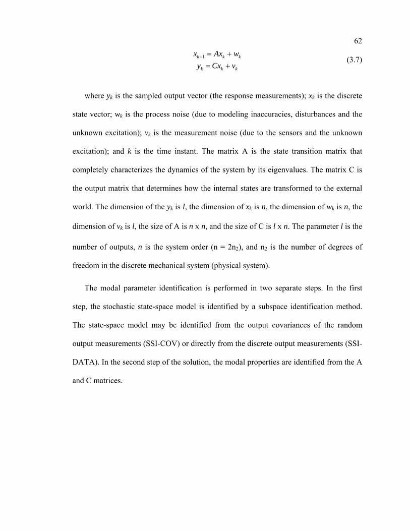
62

kkk

kkk

vCxywAxx

+=+=+1 (3.7)

where yk is the sampled output vector (the response measurements); xk is the discrete

state vector; wk is the process noise (due to modeling inaccuracies, disturbances and the

unknown excitation); vk is the measurement noise (due to the sensors and the unknown

excitation); and k is the time instant. The matrix A is the state transition matrix that

completely characterizes the dynamics of the system by its eigenvalues. The matrix C is

the output matrix that determines how the internal states are transformed to the external

world. The dimension of the yk is l, the dimension of xk is n, the dimension of wk is n, the

dimension of vk is l, the size of A is n x n, and the size of C is l x n. The parameter l is the

number of outputs, n is the system order (n = 2n2), and n2 is the number of degrees of

freedom in the discrete mechanical system (physical system).

The modal parameter identification is performed in two separate steps. In the first

step, the stochastic state-space model is identified by a subspace identification method.

The state-space model may be identified from the output covariances of the random

output measurements (SSI-COV) or directly from the discrete output measurements (SSI-

DATA). In the second step of the solution, the modal properties are identified from the A

and C matrices.

63 CHAPTER 4: AMBIENT VIBRATION TEST OF

THE BROOKLYN BRIDGE TOWERS

4.1 Introduction

This chapter describes the experimental characterization of the Brooklyn Bridge

towers by ambient vibration testing. The experimental characterization was performed to

support a seismic evaluation and retrofit investigation that was also being performed for

the bridge. The characterization consisted of identifying the dynamic properties

(frequencies and mode shapes) for the masonry towers. The measured natural frequencies

and the corresponding mode shapes of a structure are primarily a function of the mass

and stiffness characteristics and their distribution in the structure, the boundary

conditions of the structure, and the connectivity or continuity conditions between the

various subcomponents of the structure. The dynamic properties identified for the towers

from the ambient vibration test were to be used by the engineering consultant responsible

for the seismic evaluation and retrofit investigation to verify assumptions related to the

in-service conditions and behavior of the bridge, and to validate analytical models of the

bridge used to identify and assess seismic vulnerabilities and to design appropriate

countermeasures. The principal benefit expected from the experimental characterization

of the in-service structure was that the overall level of uncertainty associated with the

seismic evaluation and retrofit investigation would be significantly reduced. The

reduction in uncertainty was expected to lead to a more reliable and cost effective retrofit

design for this landmark bridge.

The focus of the experimental characterization described in this chapter was limited

to the masonry towers. The suspended spans of a symmetric half of the bridge had

64 already been experimentally characterized by both ambient and forced-vibration testing

methods as part of a previous investigation related to pedestrian vibrations. The design,

analysis and interpretation of the ambient vibration test program developed for the towers

were guided in large part by the following questions relevant to this type of suspension

bridge:

9. What is the nature of the ambient vibration environment of the entire bridge and for

its individual subcomponents?

10. What are the dynamic properties of the global system, and more importantly, of the

subcomponent towers?

11. Can the dynamic properties of the various subcomponents of the bridge be directly

extracted by measuring their respective operating vibration responses, or is it essential

to model, test, and identify the entire weakly-coupled system as an interconnected

system?

The reliability and utility of an experimental characterization of the large masonry

towers by ambient vibration testing was also considered in designing the vibration testing

program. The reliability of the experimental characterization by ambient vibration testing

was questioned given the very large mass and stiffness characteristics of the towers and

the ambient dynamic excitation levels expected to act on them. Specifically, it was not

known if the responses of the massive towers under ambient excitation would be large

enough to generate the levels of signal-to-noise ratios in the measurements necessary to

permit their dynamic properties to be reliably identified. The utility of the

characterization by ambient vibration testing for evaluating the seismic response

characteristics of the towers was also not guaranteed. The nature of any seismic

65 excitation and its transmission through the structure would be fundamentally different

from the normally dominant sources of ambient excitation such as traffic. The

discrepancy between the bandwidth and transmission characteristics of the ambient and

the design seismic excitations would certainly introduce a considerable level of

uncertainty related to the dynamic properties of the towers since these would be

identified from very low-level and likely linear responses experienced under ambient

dynamic excitation. Furthermore, the material stiffness and damping characteristics of the

tower and the behavior of the boundary conditions would be very different during a

design seismic event than under ambient dynamic excitation levels.

The design, execution and analysis of the ambient vibration testing program that was

designed and implemented for the towers of the Brooklyn Bridge are described in the

following sections of this chapter. The ambient vibration environment at the bridge is

also presented and discussed. The vibration data were analyzed using the basic peak-

picking procedure that has been used in previous experimental characterizations of other

suspension bridge towers. The results of the data analysis using this approach are

presented and discussed. It should be noted that this discussion is limited to the natural

frequencies and mode shapes identified for the towers. The damping ratios were

computed from the measurements for the various identified natural frequencies and

reported to the owner; however, these estimates should be considered somewhat

unreliable due to the very low levels of the measured responses under ambient vibration

excitation.

66 4.2 Description of the Brooklyn Bridge

The Brooklyn Bridge (Figure 4.1) crosses the East River between the Boroughs of

Manhattan and Brooklyn in New York City. The landmark structure is one New York

City’s most widely recognized icons, and is considered to be one of America’s great

national civil engineering treasures. The bridge was designed by John A. Roebling and its

construction was completed under the supervision of his son, Col. Washington Roebling.

At the time of its completion in 1883, the Brooklyn Bridge was the longest suspension

bridge in the world. The Brooklyn Bridge was also the first suspension bridge to use steel

wire instead of wrought-iron for its cables, thus it was able to support much longer and

heavier spans than its predecessors. The main bridge crossing consists of a single 1595.5

feet-long river (main) span and two 930 feet-long land (side) spans. The overall length of

the bridge, including its Manhattan and Brooklyn approach spans is 5,989 feet.

The Brooklyn Bridge features two large masonry towers (Figure 4.2) that are

supported on large-concrete-filled timber caissons. The stonework in each tower above

the waterline is granite, while limestone is used below the waterline. Each tower rises to a

height of 272.5 feet above the mean high water elevation, and is supported on large

concrete-filled timber caissons. The towers consist of three separate columns joined at

their tops by Gothic arches above the roadway deck. Additional details of the bridge are

described in Chapter 5.

67

(Drawing: Historic American Engineering Record, National Park Service, Paul Berry, 1985)(Drawing: Historic American Engineering Record, National Park Service, Paul Berry, 1985)

Figure 4.1. Overview of the Brooklyn Bridge


Figure 4.2. Overview of the Brooklyn Bridge Towers

68 4.3 Previous Dynamic Characterization of the Spans

The flexible spans of the Brooklyn Bridge were experimentally characterized prior to

the experimental characterization of the towers. This characterization was accomplished

using both ambient and forced-vibration tests on the spans of the bridge as part of a

separate investigation related to pedestrian-induced vibrations. Significant vibrations of

the flexible spans were reportedly observed as thousands of pedestrians utilized the

bridge to evacuate Manhattan (Figure 4.3) during a major electrical blackout on August

14, 2003 (Julavits, 2003). A symmetric portion of the land and river spans adjacent to the

Brooklyn Tower were tested as part of this investigation.

Forced-vibration testing was used in the investigation to obtain reliable estimates of

the damping ratios corresponding to the span modes. The forced-vibration testing was

accomplished using a large electro-hydraulic linear mass shaker that was placed at

different locations on the roadway. The linear mass shaker was able to excite a total of 18

modes in the vertical and lateral directions within the frequency range susceptible to

pedestrian induced vibrations (Kulczycki et al., 2004). The dynamic properties identified

for the spans of the bridge as a result of this investigation were also used in conjunction

with the seismic evaluation and retrofit investigation project. The focus of this

investigation was the spans, and the towers were not characterized. The very stiff and

massive towers are a critical component of the bridge with respect to seismic

performance considerations, and a similar experimental characterization of their dynamic

properties was also necessary to meet the objectives of the seismic evaluation and retrofit

investigation.

69

Figure 4.3. Pedestrians crossing the Brooklyn Bridge during electrical blackout

4.3.1 Summary Findings from the Vibration Tests of the Spans

The dynamic properties of the spans were identified by others during a previous

vibration test of the bridge (Kulczycki et al., 2004). A total of 35 modes were identified

for the bridge spans from acceleration measurements recorded on the main span and

Brooklyn side span. The frequency band of the identified modes ranged from 0.180 Hz to

2.397 Hz. The experimentally identified modes were exclusive to either the main or the

side span, and with the exception of two side span modes, they were also exclusive to the

lateral, vertical, and torsional directions of each span. The 5th lateral and 3rd torsional

modes of the side span were identified at the same frequency (1.100 Hz), and the 6th

lateral and 4th torsional modes of the side span were identified at the same frequency

(1.508 Hz). The former set of lateral and torsional modes were identified as being very

closely spaced in a 3D FE model of the bridge, while the later set of lateral and torsional

70 modes were identified at the same frequency (coupled mode) in the analytical model. The

experimentally identified modes were correlated with various analytical modes in the 3D

FE model which ranged from the 1st to the 137th mode.

4.4 Test Description

4.4.1 Proposed Test Procedure

In light of the utility and reliability considerations related to experimental

characterization of the towers by ambient vibration testing that were discussed earlier, an

experimental program was proposed for the towers that included both ambient and

forced-vibration testing was proposed to the bridge owner. The ambient vibration testing

would be used to obtain an initial identification of the natural frequencies of the tower,

and the forced-vibration testing would be performed to verify the identified frequencies,

to activate possible structural responses and behaviors at the natural frequencies that

might otherwise not be observable for ambient dynamic excitation levels, and to provide

more reliable estimates of the damping ratios at the identified natural frequencies. For

example, a properly designed forced-vibration test might reveal behaviors such as the

movement of the frozen main cable saddles or rigid body rotation of the towers about

their timber caissons. These behaviors were not necessarily expected to be observable

under the normal ambient dynamic excitation levels for the bridge.

The forced-vibration testing component of the proposed experimental program would

be performed using an eccentric mass shaker (Figure 4.4) that would be installed on the

top of the Brooklyn Tower. The engineering consultant in charge of the project (Parsons)

71 had developed preliminary analytical models of an isolated tower (Figure 4.5) that

indicated that the first three modes of the tower in the longitudinal, lateral, and torsional

directions would be near the frequency range of 1.5 to 3 Hz. The harmonic force

generated by the eccentric mass shaker varied linearly with operating frequency from

approximately 0.5 Hz to 7 Hz. The shaker could generate approximately 1,100 lbs at an

operating frequency of 1.5 Hz to a maximum of 20,000 lbs for operating frequencies

from 7 Hz to 10 Hz. The magnitudes of the harmonic forces generated by the shaker and

the resulting deflections of the tower would be relatively minor in a static sense;

however, when the operating frequency of a shaker is tuned to a natural frequency of the

structure being excited, its effect is amplified significantly.

(Photograph: Utah State University)(Photograph: Utah State University)

Figure 4.4. Eccentric mass shaker from Utah State University

72

1st Longitudinal = 1.5 Hz 1st Lateral = 2.0 Hz 1st Torsional = 2.7 Hz 1st Longitudinal = 1.5 Hz 1st Lateral = 2.0 Hz 1st Torsional = 2.7 Hz

Figure 4.5. First three tower modes from preliminary FE models

The ratio of the dynamic deflection to the static deflection for a structure under the

same magnitude of load is referred to as the dynamic load factor (Humar, 1990). The

amplitude of the dynamic load factor for an undamped structure is a maximum when the

ratio of the frequency of the exciting force to the natural frequency of the structure is

equal to one, a condition called resonance. Resonance for a damped structure is also

considered to occur when the ratio of the exciting force to the natural frequency of the

structure is equal to one, but in this case, the maximum amplitude for the dynamic load

factor occurs when the ratio of the exciting force to the natural frequency of the structure

is slightly less than one. Humar (1990) shows that when the damping ratio (ξ) is small,

the maximum amplitude will occur when the ratio of the exciting force to the natural

frequency is equal to one and the corresponding dynamic amplification factor (DAF) can

be expressed as:

73

ξ21

=DAF (4.1)

If a 2% damping ratio is assumed for each of the first three tower modes estimated

from the engineering consultant’s preliminary analytical models, the resulting dynamic

amplification factor would be 25 for each mode. This means that the force generated by

the eccentric mass shaker on the tower, when tuned to the natural frequencies of each

mode, would result in a response that would be 25 times larger than the equivalent

response for a static load of the same magnitude. The resulting amplified responses of the

tower, coupled with sensitive accelerometers, would produce a signal-to-noise ratio in the

measurements that would be more than adequate to confidently identify the resonant

frequencies.

The bridge owner ultimately decided to forgo the proposed forced-vibration testing

program and to use ambient vibration testing for the experimental characterization of the

towers due to other constraints. This was expected to lead to some uncertainty related to

the characteristics identified under very low and linear responses and the actual behavior

of the bridge, including its material behavior, stiffness and damping characteristics, and

finally its boundary conditions during a design seismic event.

4.4.2 Instrumentation Scheme

The instrumentation scheme developed for the experimental characterization by

ambient vibration testing included a stationary array of 43 uniaxial accelerometers. The

individual accelerometers were installed at various locations on the bridge to measure

vertical, longitudinal, and transverse vibration responses. The vertical and longitudinal

74 accelerometers were installed in pairs at each measurement location to permit the

torsional vibration responses to also be identified. The accelerometers were installed on

four main elements of the bridge: (1) the Brooklyn Tower (above and below the roadway

level), (2) the Manhattan Tower (below the roadway level), (3) the main span adjacent to

the Brooklyn Tower, and (4) the side span adjacent to the Brooklyn tower.

A total of 28 accelerometers were installed at different measurement levels on the

Brooklyn and Manhattan Towers as shown in Figure 4.6, Figure 4.7, and Figure 4.8. The

three independent tower columns above the roadway deck level on the Brooklyn Tower

were instrumented with two accelerometers to measure the longitudinal and transverse

(lateral) vibration responses of each column. Three accelerometers were installed at each

of the remaining levels on the towers to measure the longitudinal/torsional and transverse

vibrations. Two vertically oriented accelerometers were installed on the top of the

Brooklyn Tower and at the base of the tower. The Manhattan Tower was instrumented

with three accelerometers at a level located just below the roadway deck.

The tower accelerometers were installed using fixtures that were temporarily

anchored into the masonry stones. The accelerometers were installed at the various

measurement levels on the tower by rappelling as shown in Figure 4.9. The accelerometer

cables were routed to a data acquisition cabinet located between the stiffening trusses

under the pedestrian walkway.

Although the principal focus of the testing was the towers and the dynamic properties

of the spans had already been characterized, a limited number of accelerometers were

installed on the stiffening trusses in the main span and side span near the Brooklyn

Tower. These accelerometers were used to aid in the interpretation of the tower

75 measurements and to provide a means to correlate the tower responses with the results of

the previous span investigation. A total of 12 accelerometers were distributed between

measurement stations in the side span and main span as shown in Figure 4.10. There were

two vertically oriented accelerometers installed at the two outer trusses to measure

vertical and torsional vibration responses, and on transverse oriented accelerometer to

measure the lateral vibration responses of the spans. The arrangement of the

accelerometers on the stiffening trusses is shown in Figure 4.11. The accelerometers were

affixed to the bottom chord of the trusses using magnets. The accelerometers located at

PP31 in the side span had to be installed from the inspection walkway located between

the roadways since the motorized scaffolding system was not working in that span.

East ElevationBrooklyn Tower

(L = Longitudinal Accelerometer, T = Transverse Accelerometer, V = Vertical Accelerometer)

52’

33’

39’

54’

54’

40.5

’

272.

5’

West ElevationManhattan Tower

(L = Longitudinal Accelerometer, T = Transverse Accelerometer)

117’

D D

V TLL V

TLTLTL

TLTLTL

TLL

TLL

TLL

TLL

V VEast ElevationBrooklyn Tower

(L = Longitudinal Accelerometer, T = Transverse Accelerometer, V = Vertical Accelerometer)

52’

33’

39’

54’

54’

40.5

’

272.

5’

West ElevationManhattan Tower

(L = Longitudinal Accelerometer, T = Transverse Accelerometer)

117’

DD DD

VV TL TTLLLL VV

TL TTLLTL TTLLTL TTLL


TL TTLLLL

TL TTLLLL

TL TTLLLL

TL TTLLLL

VV VV

Figure 4.6. Measurement levels on the Brooklyn and Manhattan Towers

76

Level ATower Cross Section Below Deck Level

N

Level B & Level CTower Cross Section Below Deck Level

N

Level DTower Cross Section Below Deck Level

N

Level ETower Cross Section at Balcony Level

N

V

TL L

V

TL L

TL L

Vertical Accelerometer Longitudinal Accelerometer Transverse AccelerometerV TL


N


N


N


N

V

TL L

V

TL L

TL L


NN


NN


NN


NN

VV

TL TTTLLL LLL

VV

TL TTTLLL LLL

TL TTTLLL LLL

Vertical Accelerometer Longitudinal Accelerometer Transverse AccelerometerV TLVertical Accelerometer Longitudinal Accelerometer Transverse AccelerometerVV TTLL

Figure 4.7. Accelerometer layout at the lower measurement levels on the towers

Level F & Level GBrooklyn Tower Cross Section Above Deck Level

N

Level HTop of Brooklyn Tower

N

TL

L

V

TL TL

V

TL

Anemometer

Vertical AccelerometerV

Transverse AccelerometerT

Longitudinal AccelerometerLLevel F & Level G

Brooklyn Tower Cross Section Above Deck Level

NN

Level HTop of Brooklyn Tower

NN

TL TTTLLL

LLL

VV

TL TTTLLL TL TTTLLL

VV

TL TTTLLL

Anemometer



Longitudinal AccelerometerL

Anemometer



Longitudinal AccelerometerL

AnemometerAnemometer

Vertical AccelerometerV Vertical AccelerometerVV

Transverse AccelerometerT Transverse AccelerometerTT

Longitudinal AccelerometerL Longitudinal AccelerometerLL

Figure 4.8. Accelerometer layout at the upper measurement levels on the towers

77

Figure 4.9. Installation of accelerometers on the Brooklyn Tower

Main & Side SpansPartial Plan

PP59 PP31 PP24 PP51

Main (River) SpanSide (Land) Span

Broo

klyn

Tow

er

Brooklyn Bound Traffic

Lanes

Manhattan Bound Traffic

Lanes

Vertical Accelerometer Transverse AccelerometerV T

VT

V

VT

V

VT

V

VT

V

Main & Side SpansPartial Plan

PP59 PP31 PP24 PP51

Main (River) SpanSide (Land) Span

Broo

klyn

Tow

er

Brooklyn Bound Traffic

Lanes

Manhattan Bound Traffic

Lanes

Vertical Accelerometer Transverse AccelerometerV TVertical Accelerometer Transverse AccelerometerVV TT

VT VVTT

VV

VT

V

VT VVTT

VV

VT

V

VT VVTT

VV

VT

V

VT VVTT

VV

Figure 4.10. Locations of the measurement stations for the spans

78

Stiffening Trusses PP51, PP24 & PP59

Manhattan Bound Roadway

Brooklyn Bound Roadway

Pedestrian Walkway

Out

er T

russ

Inne

r Tru

ss

Inne

r Tru

ss

Out

er T

russ

33’-0” 33’-0”16’-6”

N

Stiffening Trusses PP31



Pedestrian Walkway

Out

er T

russ

Inne

r Tru

ss

Inne

r Tru

ss

Out

er T

russ

33’-0” 33’-0”16’-6”

N

VTV

VTV

Vertical Accelerometer

Transverse Accelerometer

V

T

Stiffening Trusses PP51, PP24 & PP59



Pedestrian Walkway

Out

er T

russ

Inne

r Tru

ss

Inne

r Tru

ss

Out

er T

russ

33’-0” 33’-0”16’-6”

NN

Stiffening Trusses PP31



Pedestrian Walkway

Out

er T

russ

Inne

r Tru

ss

Inne

r Tru

ss

Out

er T

russ

33’-0” 33’-0”16’-6”

NN

VT VVVTTVVV

VT VVVTTVVV



V

T



V

T



VV

TT

Figure 4.11. Arrangement of the accelerometers on the stiffening trusses

4.4.3 Sensors and Data Acquisition

The instrumentation scheme developed for the ambient vibration test of the Brooklyn

Bridge included sensors for measuring the vibration responses of the bridge components,

an anemometer for measuring the wind speed and direction, and a temperature sensor to

measure the ambient temperature at the bridge. The sensors were installed at various

locations on the bridge, and their cables were all routed to a single data acquisition

cabinet located on the bridge. The installed sensors were left in place on the bridge

79 throughout the duration of the ambient vibration testing program. The specific

characteristics of the sensors and data acquisition system that were used for the

experimental program are described in the following sections.

4.4.3.1 Accelerometers

There were two different types of accelerometers used to measure the vibration

responses of the Brooklyn Bridge during the ambient vibration testing. These included

piezoelectric and capacitive type accelerometers from PCB Piezoelectronics Inc. Both

types of accelerometers are shown in Figure 4.12.

The piezoelectric accelerometer used was the Model 393C seismic accelerometer.

This accelerometer uses the piezoelectric effect of quartz to directly convert acceleration

to a low impedance voltage signal. The voltage signal produced is proportional to the

vibratory force experienced by the accelerometer. The low-impedance output signal can

be transmitted over very long distances with minimal signal degradation using regular

coaxial cable. The stainless steel sensor housing is hermetically sealed and contains the

crystals, a seismic mass, and a low noise electronic amplifier. The Model 393C

accelerometer is a unidirectional sensor; therefore, it can only measure accelerations in

one principal direction. A total of 27 of these accelerometers were used for the ambient

vibration test. The specific performance characteristics of this sensor are summarized in

Table 4.1.

The Model 3701 accelerometer was the capacitive type of accelerometer used for the

ambient vibration testing. This accelerometer uses an air-damped, opposed-plate

capacitor and the sensing element. Once energized, the accelerometer generates a low-

80 impedance voltage output that is directly proportional to acceleration. The low-

impedance output signal can be transmitted over long distances with minimal signal

degradation using ordinary wires. Capacitive accelerometers can measure frequencies all

the way to DC (0 Hz). The tolerances of the internal electrical components give this

accelerometer a zero-g offset voltage. The voltage offset is generally less than 200 mV

and could be nulled by the zero-adjust feature on the capacitive accelerometer signal

conditioners. The Model 3701 accelerometer requires a three-conductor cable, with one

conductor to carry the excitation power, one conductor for carrying the measurement

signal, and the final conductor serving as a common ground. This particular

accelerometer is also a unidirectional sensor. A total of 16 of these capacitive

accelerometers were used for the ambient vibration test. The performance characteristics

for the Model 3701 accelerometer are also listed in Table 4.1.

The accelerometer manufacturer supplied a factory calibrated value for the sensitivity

of each sensor. These values were verified in the laboratory using the back-to-back

calibration method before the sensors were installed on the bridge. In the back-to-back

method of calibration, the accelerometer being calibrated is placed back-to-back with a

working reference standard accelerometer and installed on a shaker. The two

accelerometers are subjected to the same acceleration at different frequencies and the

ratio of their sensitivities at each frequency is equal to the ratio of their outputs.

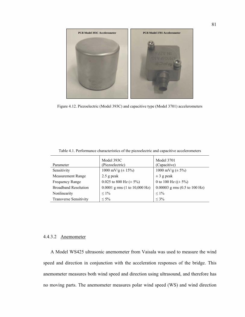
81 PCB Model 393C Accelerometer PCB Model 3701 AccelerometerPCB Model 393C Accelerometer PCB Model 3701 Accelerometer

Figure 4.12. Piezoelectric (Model 393C) and capacitive type (Model 3701) accelerometers

Table 4.1. Performance characteristics of the piezoelectric and capacitive accelerometers

Parameter Model 393C (Piezoelectric)

Model 3701 (Capacitive)

Sensitivity 1000 mV/g (± 15%) 1000 mV/g (± 5%) Measurement Range 2.5 g peak ± 3 g peak Frequency Range 0.025 to 800 Hz (± 5%) 0 to 100 Hz ((± 5%) Broadband Resolution 0.0001 g rms (1 to 10,000 Hz) 0.00003 g rms (0.5 to 100 Hz) Nonlinearity ≤ 1% ≤ 1% Transverse Sensitivity ≤ 5% ≤ 3%

4.4.3.2 Anemometer

A Model WS425 ultrasonic anemometer from Vaisala was used to measure the wind

speed and direction in conjunction with the acceleration responses of the bridge. This

anemometer measures both wind speed and direction using ultrasound, and therefore has

no moving parts. The anemometer measures polar wind speed (WS) and wind direction

82 (WD) relative to a north reference that is engraved on the top of the sensor. The

anemometer was installed on top of the Brooklyn Tower (north end) as shown in Figure

4.13, and was oriented so that the sensor’s north reference pointed towards Manhattan

and was parallel to the length of the bridge. This orientation means that the wind

direction was acting perpendicular to the length of the bridge when the measured WD

value was either 90 degrees or 180 degrees.

Figure 4.13. Ultrasonic anemometer on top of the Brooklyn Tower

83 4.4.3.3 Data Acquisition System

The data acquisition system used for the project consisted of three basic hardware

components: (1) multi-channel accelerometer signal conditioners from PCB

Piezoelectronics Inc., (2) a Model E8401A VXI mainframe with Model E1432A input

modules from Agilent Technologies, and (3) a laptop computer. Figure 4.14 shows the

inter-connections between the accelerometers and the data acquisition hardware

components.

The signal conditioners used were specific to each type of accelerometer. A single

Model 478A16 signal conditioner was used for the capacitive accelerometers, and two

Model 481 signal conditioners were used for the piezoelectric accelerometers. Each

signal conditioner could accommodate 16 accelerometers and supplied the regulated

excitation voltage required for the accelerometers.

The analog to digital conversion of the acceleration signals is accomplished using

Model E1432A input modules which are installed in open slots of the VXI mainframe.

Each input module is a 16 channel, 51.2 kSamples/s digitizer with DSP (Digital Signal

Processing). The input modules have 16 bit resolution for amplitude and dynamic range.

This data acquisition system is equipped with buffers to be able to simultaneously sample

multiple accelerometers across multiple input modules and at high speeds. The DSP

permits acceleration measurements to be collected using AC or DC coupling. When AC

coupling is selected, the measurement data is high pass filtered at 1 Hz by the input

module prior to storage. When the measurements are collected using DC coupling, the

data is not high pass filtered prior to storage and frequencies down to DC (0 Hz) are

84 observable. Since some of the natural frequencies for the Brooklyn Bridge spans were

expected to be less than 1 Hz, DC coupling was selected for the measurements.

A short patch cable (RG58U Coax) connected each output channel from the signal

conditioners to breakout boxes connected to the input modules on the VXI mainframe. A

laptop computer connected to the VXI mainframe was used to control the data acquisition

system and to store the measurement data.

The data acquisition components were placed in a watertight cabinet located on the

inspection walkway adjacent to the Brooklyn tower as shown in Figure 4.15. Two

different types of lead wires were used to connect the accelerometers to the signal

conditioners. Individually shielded, twisted pair cables (2 pair cable) were used to

connect the capacitive accelerometers to their signal conditioner, and RG58U coaxial

cables were used to connect the piezoelectric accelerometers to their signal conditioners.

A separate lead wire was run from each accelerometer installed on the bridge to the

cabinet containing the data acquisition hardware components.

4.4.4 Test Execution

The ambient vibration testing was conducted over a period of about one month. The

data acquisition system was manually operated from the bridge so that the measurement

parameters could be adjusted to ensure optimal performance and accuracy during the

changing ambient excitation and environmental conditions. The data acquisition system

was also set to operate while unattended during evenings and weekends. The ambient

temperature was periodically measured and recorded while the data acquisition system

was being operated manually. The accelerations were primarily measured at either 20

85 samples/second (20 Hz) or 40 samples/second (40 Hz), and were recorded in time periods

ranging from 30 minutes to about 3 days in length.

Model E8401A VXI Mainframe with Model E1432A 16-Channel

Input Modules

Piezoelectric Accelerometers

Capacitive Accelerometers

Laptop Computer

Capacitive Signal Conditioner

Sensor Lead Wires(RG58U Coax)

Sensor Lead Wires(2 Pair Cables)

ICP Signal Conditioner

Short Patch Cables(RG58U Coax)

Short Patch Cables(RG58U Coax)Model E8401A VXI Mainframe

with Model E1432A 16-Channel Input Modules

Piezoelectric Accelerometers

Capacitive Accelerometers

Laptop Computer

Laptop Computer

Capacitive Signal Conditioner

Sensor Lead Wires(RG58U Coax)

Sensor Lead Wires(2 Pair Cables)

ICP Signal Conditioner



Figure 4.14. Data acquisition system components

Figure 4.15. Data acquisition cabinet on inspection walkway

86 4.5 Data Processing and Analysis

4.5.1 Data Pre-Processing

The data pre-processing consisted of a number of steps that served to ensure the

quality of each measured acceleration signal and to prepare these signals for subsequent

data processing steps needed to identify the dynamic properties (frequencies and mode

shapes) for the towers. The data pre-processing procedure applied to the measurement

data included the following steps:

12. Data quality analysis

13. Data filtering

14. Signal cleaning

15. De-coupling of combined vibration responses

The first three steps were used to evaluate the quality of the signals recorded by each

output sensor channel. They were performed in an iterative manner until the resulting

signals were judged to be relatively clean from noise and bias type errors. The data

quality analysis that was performed was a somewhat subjective process that involved

visually examining the raw time domain signals from each output sensor channel and

their resulting frequency domain transformations. The identification and removal of noise

and bias errors from the raw time domain signals was a critical step since if these errors

are significant, they can lead to erroneous estimates of the identified modal properties

during the subsequent data analysis stage. The purpose of the final step in the pre-

processing stage was to decouple the combined vertical/torsional responses of the spans

and the combined longitudinal/torsional responses of the towers into discrete

87 representations of purely vertical, longitudinal, and torsional vibration responses. The

procedures employed in each of these steps are further described in following sections.

4.5.1.1 Data Quality Analysis

The quality of the data was evaluated by visually inspecting the raw (untreated) time

domain signals (acceleration versus time) for each channel. A Fast Fourier

Transformation (FFT) was also computed from the raw time domain signal from each

output channel during this step. The time and frequency domain signals for each output

sensor channel were examined to identify any noisy or malfunctioning sensors. The

locations of any spurious noise spikes in the time domain signals were also noted and

recorded for use in the subsequent cleansing of the signals. The frequency domain signals

were inspected to establish the frequency range that contained the majority of the

significant responses.

4.5.1.2 Data Filtering

The signals were band pass filtered to remove any DC (zero Hz) bias or drift from the

signals, and to minimize the effects of high frequency components in the frequency band

of interest. The frequency domain signals indicated that the most of the vibration

responses for the towers were located in the frequency band between 1 Hz and 5 Hz. The

majority of the vibration responses for the span were located in a similar frequency band,

but with some responses occurring at frequencies below 1 Hz. Based on these

observations, the cutoff frequencies selected for the digital filter were 0.3 Hz at the low

end and 10 Hz at the upper end of the spectrum. It was expected that these cutoff

88 frequencies would retain the majority of the vibration responses for the towers. The

digital filter used in this step was a 5th order Butterworth Filter, and this operation was

performed in Matlab.

4.5.1.3 Signal Cleaning

The data quality analysis identified one accelerometer channel that did not function

correctly during the ambient vibration testing. The non-functioning sensor was a

longitudinal accelerometer located at Level F on the Brooklyn Tower (on the north tower

column). This accelerometer was excluded from the subsequent data processing and

analysis.

The visual inspection of the raw time domain signals from the output sensor channels

also revealed that the responses for some output channels contained very large (relative to

the rest of the response) but isolated peaks in the time records, while the responses for

others channels contained isolated peaks that were smaller relative the rest of the

response record. The time domain response signals were generally of a more reasonable

character between these isolated peaks. Typical examples of both the large and small

isolated or spurious responses observed in the time domain signals of different output

channels are shown in Figure 4.16. In most cases, there was no discernable pattern

associated with the observed spurious responses. The spurious responses would occur at

simultaneously for some channels at some point in the time history and occur in different

channels at different times at other points in the time history. The spurious responses

were not limited to only a certain group of output channels.

89 The spurious responses in the time history of each channel were removed in order to

preserve the maximum amount of acceptable responses for use in subsequent stages of

the data analysis process. The portions of the time histories corresponding to occurrences

of spurious responses were eliminated across all channels in the data set. The portions of

the time record were removed from all channels even if the response for a certain channel

was acceptable to preserve the phase relationships between the acceleration responses

recorded by each channel.

Three different approaches for combining the remaining portions of clean response

were evaluated to investigate their effect on the subsequent data analysis. These different

approaches were evaluated by computing the autospectral densities (ASD) for each

approach and comparing the results. The different approaches for combining the cleaned

records may be described in conjunction with the accelerometer time history containing

spurious responses shown in Figure 4.17. The portion of the acceleration response shown

in this figure contains three instances of spurious responses. The portions of the

acceleration record from every acceleration channel corresponding to these spurious

responses were eliminated from the records. As a result, there were four regions left from

the original records of each output channel containing clean response (Segments A, B, C,

and D in Figure 4.17). Of the remaining portions of the signals, only Segments A, B, and

D contained enough data points to compute the ASD using a consistent resolution with no

zero-padding required.

The first approach evaluated for combining the clean signals was to compute the ASD

for Segments A, B, and D, and then take the average of the results. The second approach

was simply to combine Segments A, B, and D in the time domain by placing them end to

90 end, and to compute the ASD for the resulting composite time domain signals. The final

approach evaluated was to combine all of the clean segments (Segments A, B, C, and D)

in the time domain and compute the ASD for the resulting composite time domain

signals.

The ASD computed using the these three approaches for combining the cleaned

portions of the time domain signals are shown with the original time domain signal (non-

cleaned) for three different output channels containing large, small and no spurious peaks

in Figure 4.18, Figure 4.19 and Figure 4.20, respectively. It is clear from these figures

that the large spurious peaks, if not removed, have the most significant effect on the

resulting ASD. It is also clear from these figures that there is not much difference

between the ASDs computed using the different approaches for combining the clean

portions of the signal. The third approach was selected for use in combining the cleaned

portions of each record for subsequent stages of the data analysis since it was the easiest

method to program.

91

3.8565 3.857 3.8575 3.858 3.8585 3.859

x 105

-0.02

-0.01

0

0.01

0.02

Filtered Time Domain Data for Brooklyn Tower Longitudinal Accelerometers

Sample Number

Acc

eler

atio

n (g

)

13151619202324

1.656 1.6562 1.6564 1.6566 1.6568 1.657 1.6572 1.6574 1.6576

x 105

-2

-1

0

1

x 10-3 Filtered Time Domain Data for Brooklyn Tower Transverse Accelerometers

Sample Number

Acc

eler

atio

n (g

)

12141718212225

Tower Longitudinal Accelerations

Tower Transverse Accelerations

Large Spike

Small Spike

3.8565 3.857 3.8575 3.858 3.8585 3.859

x 105

-0.02

-0.01

0

0.01

0.02

Filtered Time Domain Data for Brooklyn Tower Longitudinal Accelerometers

Sample Number

Acc

eler

atio

n (g

)

13151619202324

1.656 1.6562 1.6564 1.6566 1.6568 1.657 1.6572 1.6574 1.6576

x 105

-2

-1

0

1

x 10-3 Filtered Time Domain Data for Brooklyn Tower Transverse Accelerometers

Sample Number

Acc

eler

atio

n (g

)

12141718212225

Tower Longitudinal Accelerations

Tower Transverse Accelerations

Large Spike

Small Spike

Figure 4.16. Large and small spurious spikes in the raw time domain acceleration records

1000 2000 3000 4000 5000 6000

-4

-2

0

2

4

6x 10

-3 Filtered Time Domain Data with Noise for Channel 13

Time (sec)

Acc

eler

atio

n (g

)

Typical spurious responses

Portions of record removed during cleansing (from all

output channels)

Segment “A” Segment “B” Segment “D”

Segment “C”

1000 2000 3000 4000 5000 6000

-4

-2

0

2

4

6x 10

-3 Filtered Time Domain Data with Noise for Channel 13

Time (sec)

Acc

eler

atio

n (g

)

Typical spurious responses

Portions of record removed during cleansing (from all

output channels)

Segment “A” Segment “B” Segment “D”

Segment “C”

Figure 4.17. Removal of spurious responses from acceleration record

92

0 5000 10000 15000-0.015

-0.01

-0.005

0

0.005

0.01

0.015Filtered Time Domain Data with Noise for Channel #12

Time (sec)

Acc

eler

atio

n (g

)

0 1 2 3 4 5 610-12

10-10

10-8

10-6

PSD for Channel #12

Frequency (Hz)

PS

D (

g2 /Hz)

W ith NoiseAvg of SegementsComposite of Valid SegmentsComposite of All Segments

Original Signal with Large Spurious Peaks

Average ASDASD for Composite of A, B and DASD for Composite of all segments

Original Signal

Autospectral Densities (ASD) for CH 12

0 5000 10000 15000-0.015

-0.01

-0.005

0

0.005

0.01

0.015Filtered Time Domain Data with Noise for Channel #12

Time (sec)

Acc

eler

atio

n (g

)

0 1 2 3 4 5 610-12

10-10

10-8

10-6

PSD for Channel #12

Frequency (Hz)

PS

D (

g2 /Hz)


Original Signal with Large Spurious Peaks


Original SignalAverage ASDASD for Composite of A, B and DASD for Composite of all segments

Original Signal


Figure 4.18. Effect of different combination methods for channel with large spurious peaks

0 5000 10000 15000-6

-4

-2

0

2

4

6x 10-4 Filtered Time Domain Data with Noise for Channel #43

Time (sec)

Acc

eler

atio

n (g

)

0 1 2 3 4 5 610-12

10-10

10-8

10-6

PSD for Channel #43

Frequency (Hz)

PS

D (

g2 /Hz)


Original Signal with Small Spurious Peaks


Original Signal


0 5000 10000 15000-6

-4

-2

0

2

4


Time (sec)

Acc

eler

atio

n (g

)

0 1 2 3 4 5 610-12

10-10

10-8

10-6

PSD for Channel #43

Frequency (Hz)

PS

D (

g2 /Hz)


Original Signal with Small Spurious Peaks

0 5000 10000 15000-6

-4

-2

0

2

4


Time (sec)

Acc

eler

atio

n (g

)

0 1 2 3 4 5 610-12

10-10

10-8

10-6

PSD for Channel #43

Frequency (Hz)

PS

D (

g2 /Hz)


Original Signal with Small Spurious PeaksOriginal Signal with Small Spurious Peaks



Original Signal


Figure 4.19. Effect of different combination methods for channel with small spurious peaks

93

0 5000 10000 15000-1

-0.5

0

0.5

1

1.5x 10-3 Filtered Time Domain Data with Noise for Channel #23

Time (sec)

Acc

eler

atio

n (g

)

0 1 2 3 4 5 610-12

10-10

10-8

10-6

PSD for Channel #23

Frequency (Hz)

PS

D (

g2 /Hz)


Original Signal with no Spurious Peaks


Original Signal


0 5000 10000 15000-1

-0.5

0

0.5

1

1.5x 10-3 Filtered Time Domain Data with Noise for Channel #23

Time (sec)

Acc

eler

atio

n (g

)

0 1 2 3 4 5 610-12

10-10

10-8

10-6

PSD for Channel #23

Frequency (Hz)

PS

D (

g2 /Hz)


Original Signal with no Spurious Peaks



Original Signal


Figure 4.20. Effect of different combination methods for channel with no spurious peaks

4.5.1.4 Decoupling of Combined Vibration Responses

The final step in the data pre-processing stage was to decouple the combined

vertical/torsional vibration responses for the spans and the combined

longitudinal/torsional responses for the towers into their pure vertical, longitudinal, and

torsional responses. The pure vertical responses were decoupled from the combined

responses by summing the response of the two vertical accelerometers located on the two

outer trusses at each measurement station on the main and side spans. The pure

longitudinal responses were decoupled from the combined responses for the towers by

summing the responses from the two longitudinal accelerometers located at each

94 measurement level on the towers. The pure torsional vibration responses of the spans and

towers were computed by subtracting the response of one vertical (or longitudinal)

channel from the other vertical (or longitudinal) channel at each measurement station on

the spans and towers.

4.5.2 Modal Parameter Identification by Peak-Picking Method

The frequencies and mode shapes were identified from the measured responses using

the common peak-picking (PP) method. In the PP method, the modal properties can be

identified using the information available in the autospectral density (ASD) functions,

cross spectral density (CSD) functions, and ordinary coherence functions as outlined by

Bendat and Piersol (1980). The natural frequencies were identified from the locations of

peaks in the autospectral density functions estimated for each measured acceleration

response. The mode shapes at the identified spectral peak may be estimated from the

magnitude and phase information contained in the CSD function estimated between

response in a particular direction at each measurement location and the response in the

same direction at a selected reference response location. The mode shapes estimated from

the measurement data are in reality operating deflection shapes. An operating deflection

shape is a deflection shape that may include the contributions of more than one mode in

the vicinity of the spectral peak; however, if the modes are not too closely-spaced and if

the damping ratios are small, the operating deflection shapes will be reasonable

approximations of the undamped mode shapes. The ordinary coherence function is also

computed between each response and the reference response location to aid in the

identification of the natural frequencies.

95 The natural frequencies and mode shapes were identified for the Brooklyn Tower in

the longitudinal, lateral and torsional response directions. Mode shapes were not

estimated for the span or the Manhattan Tower measurements since the number of

measurement locations that were permitted for these components was not sufficient to

overcome spatial aliasing in the mode shape estimates. The ASD functions were

estimated for these locations and used to identify the frequencies corresponding to

spectral peaks. The frequencies of the spectral peaks from the span and Manhattan Tower

measurement locations were used in conjunction with interpreting the results from the

Brooklyn Tower.

4.5.2.1 Estimation of Autospectral Density and Cross Spectral Density Functions

The ASD and CSD functions were estimated using Welch’s average modified

periodogram method. The specifics of the computations required for estimating the ASD,

CSD, and ordinary coherence functions from discrete time domain data are described in

Chapter 6. The ASD and CSD estimates were computed from the pre-processed data

using 50% overlap processing and a Hanning Window to minimize spectral leakage

effects. The blocksize used in computing these estimates for the data sampled at 40 Hz

was 8192 points, which gave a frequency resolution of 0.0049 Hz. The same frequency

resolution was obtained for the data sets that were sampled at 20 Hz by using a blocksize

of 4096 points. This frequency resolution was expected to be more than adequate to

resolve any closely-spaced natural frequencies.

96 4.5.2.2 Identification of Natural Frequencies and Mode Shapes

The frequencies corresponding to the locations of spectral peaks in the ASD functions

for each tower response should theoretically correspond to the natural frequencies of the

towers. In order to simplify the identification of the spectral peak locations for each

response direction, the responses were first combined into several different mode

indicator functions (MIFs). The MIFs that were computed and used for the tower

responses included the Average Normalized Power Spectral Density (ANPSD) function

that was developed by Felber (1993), and one additional MIF termed the SPSD which

was developed for use in this project.

The ANPSD function is determined by first computing the autospectral density

(ASD), which is also called the Power Spectral Density (PSD), for each output channel.

The resulting ASD functions are then normalized by dividing the ASD value at each

frequency line by the sum of the ASD values at all frequency lines. The normalized ASD

values at each frequency line from each output channel are then summed and the

resulting value is divided by the number of output channels used. The equations used to

compute the ANPSD are given in Chapter 6. The SPSD is a somewhat simplified

variation of the ANPSD function in that it simply takes the sum of the ASD values at

each frequency line for the output channels. The SPSD does not employ any

normalization or averaging of the ASD values. The equations used to compute the SPSD

are also given in Chapter 6.

A separate MIF was computed for each tower response direction (longitudinal,

torsional, and lateral). The peaks were identified in an automated manner by comparing

the amplitude of the MIF at a given frequency line with the amplitude at the five adjacent

97 frequency lines immediately before and after the frequency line being evaluated. This so-

called 5P selection criterion is illustrated in Chapter 6 by Figure 6.12. A minimum MIF

amplitude level criterion was also applied for the automated identification of the spectral

peak locations. The minimum MIF amplitude level criterion served to filter out any

spectral peak locations associated with low signal-to-noise ratios. The minimum level

threshold criterion is illustrated by Figure 6.13 in Chapter 6.

The mode shapes were computed at every frequency line from the magnitude and

phase information contained in the CSD computed between each output channel in a

given response direction and a selected reference output channel. In this project, the

longitudinal, torsional, and lateral responses near the roadway deck level of the bridge

(Level E in Figure 4.6). A single tower level was selected to serve as the reference as was

done in earlier characterizations of suspension bridge towers by ambient vibration testing

(Abdel-Ghaffar and Scanlan, 1985; Brownjohn, et al., 1987; Brownjohn, et al., 1989,

Brownjohn, et al., 1992). In this case, the selected reference location was at the roadway

deck level, which was similar to the selected reference level used in the characterization

of the Golden Gate Bridge towers (Abdel-Ghaffar and Scanlan, 1985). In the other tower

characterizations by ambient vibration testing referenced above, accelerometers that were

located at the tops of the towers served as the reference sensors.

The phase information between each measurement level and the reference level were

forced to have values of either zero or 180 degrees. This constrained the mode shapes

computed at each frequency line to behave as a normal mode. Computed phase factors

between zero and +/-90 degrees were forced to a value of zero degrees (in-phase with the

reference level), and the computed phase factors that were between 90 and 180 (or

98 between -90 and -180 degrees) were forced to a value of 180 degrees (out-of-phase with

the selected reference level). The original unmodified values of the phase factor were

later checked to confirm normal mode behavior (phase factors very close to zero or 180

degrees) for identified spectral peaks that were considered as possible modes of the

structure.

The ordinary coherence function was also computed between the output from each

measurement level on the tower and the selected reference level. The computations

necessary to estimate the ordinary coherence function are given in Chapter 6. The

ordinary coherence function will have values between 0 and 1, and the maximum values

occurring near natural frequencies of the system (Bendat and Piersol, 1980). The values

of the ordinary coherence function computed for each measurement level on the tower

relative to the reference level were summed at each frequency line and expressed as a

percentage of their maximum possible value (%SCOH). For example, if the sum of the

ordinary coherence values for five output responses relative to a reference response is

equal to 4.5 for a given frequency line, the resulting %SCOH value would be computed

to be 90%.

4.6 Results

The results shown in the following sections were computed from one data set

recorded during the ambient vibration testing program on the bridge. The acceleration

measurements contained in this data set were sampled at 40 Hz, and the total duration of

the vibration monitoring for this data set was 4 hours. The measurements were recorded

on November 22, 2004 between 4:00 pm and 8:00 pm. This particular data set was

99 selected for analysis since it contained some unusually large amplitude accelerations for

the tower channels, and particularly for the transverse (lateral) response direction.

4.6.1 Amplitudes of Acceleration Signals

There were significant differences in the amplitudes of the recorded accelerations

from the different components of the bridge (the spans and the towers) and for the

different response directions (longitudinal or vertical and transverse). The vibration

amplitudes were generally largest for the vertical accelerometers that were located on the

flexible spans. The vibration amplitudes measured by longitudinal accelerometers that

were located on the towers were smaller than for the vertical accelerometers on the spans,

but were larger than the lateral responses of the spans. Figure 4.21 shows examples of the

vertical acceleration responses from the main span, and the longitudinal response at the

top of the Brooklyn Tower. Figure 4.22 shows the typical lateral vibration responses at

for the same two locations shown in the previous figure. The amplitudes of the span

accelerations were generally nearly twice as large in the vertical direction as they were in

the lateral direction at the same measurement location. Similarly, the amplitudes of the

measured longitudinal accelerations for the tower were generally twice as large as those

in the lateral direction. The lateral responses of the spans were at least an order of

magnitude larger than the lateral responses for the tower.

100

1 1.05 1.1 1.15 1.2 1.25 1.3 1.35 1.4 1.45 1.5

x 104

-0.01

-0.005

0

0.005

0.01

Time (sec)

Acc

eler

atio

n (g

)

Tower Longitudinal

1 1.05 1.1 1.15 1.2 1.25 1.3 1.35 1.4 1.45 1.5

x 104

-0.015

-0.01

-0.005

0

0.005

0.01

0.015

Time (sec)

Acc

eler

atio

n (g

)

Main Span Vertical

Level H

PP51

4x10-4

-4x10-4

1 1.05 1.1 1.15 1.2 1.25 1.3 1.35 1.4 1.45 1.5

x 104

-0.01

-0.005

0

0.005

0.01

Time (sec)

Acc

eler

atio

n (g

)

Tower Longitudinal

1 1.05 1.1 1.15 1.2 1.25 1.3 1.35 1.4 1.45 1.5

x 104

-0.015

-0.01

-0.005

0

0.005

0.01

0.015

Time (sec)

Acc

eler

atio

n (g

)

Main Span Vertical

Level H

PP51

4x10-4

-4x10-4

Figure 4.21. Acceleration amplitudes for vertical span and longitudinal tower vibrations

101

1 1.05 1.1 1.15 1.2 1.25 1.3 1.35 1.4 1.45 1.5

x 104

-4

-2

0

2

4x 10-4

Time (sec)

Acc

eler

atio

n (g

)

Tower Lateral

1 1.05 1.1 1.15 1.2 1.25 1.3 1.35 1.4 1.45 1.5

x 104

-3

-2

-1

0

1

2

3x 10-3

Time (sec)

Acc

eler

atio

n (g

)

Main Span Lateral

Level H

PP51

Figure 4.22. Acceleration amplitudes for lateral span and tower vibrations

4.6.2 Spectral Content of Acceleration Signals

The autospectral densities computed for the different measurement levels of the

towers for longitudinal, torsional, and lateral vibrations are shown in Figure 4.23 and

Figure 4.24. These figures show that there are numerous spectral peaks in the frequency

range of 0 Hz to 2 Hz in the longitudinal response. The torsional response also shows

multiple spectral peaks in the slightly larger frequency range of 0 Hz to 3 Hz. The

preliminary analytical models of the bridge indicated that there were most likely three

102 tower modes in the frequency range between 0 Hz and 3 Hz, so many of the peaks

contained in these spectral were likely to represent spurious results that correspond to

something other than the natural frequencies of the towers.

The ASD for the lateral responses of the tower has spectral peaks that are mostly

between 1 Hz and 5 Hz. The ASD for the lateral tower responses shows several large

spectral peaks near 5 Hz. These peaks were believed to be the result of some unusual

excitation for the bridge. These peaks can also be seen in Figure 4.23 for the ASDs of the

tower longitudinal and torsional responses although their magnitudes are relatively

smaller than the other spectral peaks at the lower end of the frequency band.

The autospectral densities computed for the vertical, torsional and lateral vibrations of

the main and side spans in the vicinity of the Brooklyn Tower are given in Figure 4.25

and Figure 4.26. It is clear from Figure 4.25 that there are many more spectral peaks for

the vertical and torsional vibrations of the spans than were observed for the tower

responses. The spectral peaks are also better distributed across the frequency band from 0

Hz to 5 Hz. Many of the spectral peaks for these responses occur at the same frequencies

as the spectral peaks shown in Figure 4.23 for the longitudinal vibration responses of the

Brooklyn Tower. As shown in Figure 4.26, the spectral peaks for the lateral vibration

responses of the spans are mostly at frequencies less than 2 Hz.

103

0 0.5 1 1.5 2 2.5 3 3.5 4 4.5 50

0.5

1

1.5

2

2.5

3

3.5

4

4.5x 10-7

Frequency (Hz)

Acc

eler

atio

n (g

2 /Hz)

BCEGHMT

0 0.5 1 1.5 2 2.5 3 3.5 4 4.5 50

1

2

3

4

5

6

7x 10-8

Frequency (Hz)

Acc

eler

atio

n (g

2 /Hz)

BCEGHMT

Tower Longitudinal Response

Tower Torsional Response

Figure 4.23. Autospectral densities for longitudinal and torsional vibrations of the towers

104

0 0.5 1 1.5 2 2.5 3 3.5 4 4.5 50

0.2

0.4

0.6

0.8

1

1.2

1.4x 10

-8

Frequency (Hz)

Acc

eler

atio

n (g

2 /Hz)

BCEF-NF-SF-MG-SG-MHMT

Tower Lateral Responses

0 0.5 1 1.5 2 2.5 3 3.5 4 4.5 50

0.2

0.4

0.6

0.8

1

1.2

1.4x 10

-8

Frequency (Hz)

Acc

eler

atio

n (g

2 /Hz)

BCEF-NF-SF-MG-SG-MHMT

Tower Lateral Responses

Figure 4.24. Autospectral densities for lateral (transverse) vibrations of the towers

105

0 0.5 1 1.5 2 2.5 3 3.5 4 4.5 50

0.5

1

1.5

2

2.5x 10

-5

Frequency (Hz)

Acc

eler

atio

n (g

2 /Hz)

MS-24MS-51SS-31SS-59

0 0.5 1 1.5 2 2.5 3 3.5 4 4.5 50

0.5

1

1.5

2

2.5

3

3.5

4x 10

-5

Frequency (Hz)

Acc

eler

atio

n (g

2 /Hz)


Span Vertical Responses

Span Torsional Responses

0 0.5 1 1.5 2 2.5 3 3.5 4 4.5 50

0.5

1

1.5

2

2.5x 10

-5

Frequency (Hz)

Acc

eler

atio

n (g

2 /Hz)


0 0.5 1 1.5 2 2.5 3 3.5 4 4.5 50

0.5

1

1.5

2

2.5

3

3.5

4x 10

-5

Frequency (Hz)

Acc

eler

atio

n (g

2 /Hz)


Span Vertical Responses

Span Torsional Responses

Figure 4.25. Autospectral densities for the vertical and torsional vibrations of the main and side spans

106

0 0.5 1 1.5 2 2.5 3 3.5 4 4.5 50

0.2

0.4

0.6

0.8

1

1.2x 10

-6

Frequency (Hz)

Acc

eler

atio

n (g

2 /Hz)


Main and Side Span Lateral Responses

0 0.5 1 1.5 2 2.5 3 3.5 4 4.5 50

0.2

0.4

0.6

0.8

1

1.2x 10

-6

Frequency (Hz)

Acc

eler

atio

n (g

2 /Hz)


Main and Side Span Lateral Responses

Figure 4.26. Autospectral densities for the lateral vibrations of the main and side spans

4.6.3 Time Variation of Spectral Content

In order to characterize the ambient vibration environment for the different

components of the bridge, it is helpful to examine how the spectral content at each

measurement location varies with time. It is usually assumed in ambient vibration testing

that both the structure and the excitation are stationary. In other words, it is assumed that

the characteristics of the structure remain constant as does the frequency content of the

ambient dynamic excitation. The assumed stationarity of the structure and excitation has

107 been shown to be not very realistic for vibration tests of short to medium span bridges

(Farrar et al., 1994; Fu and DeWolf, 2001; Peeters et al, 2001).

The time variation of the spectral content for the longitudinal, torsional, and lateral

vibrations at different levels on the towers are shown in Figure 4.27, Figure 4.28 and

Figure 4.29, respectively. The majority of the significant spectral content for the tower

vibrations was located in the 0 to 5 Hz frequency band. The response at Level F is

excluded from these figures since one of the longitudinal accelerometers at this level

ceased functioning during the test and the logistics of the sensor installation did not

permit it to be replaced. The intensity of the vibration at a given frequency line is

indicated by the level of shading in the graphs with the darkest regions corresponding to

the largest vibration amplitudes. It can also be seen from the figures that the measured

vibration amplitudes were generally largest at the top of the tower.

The lateral response at the top of the Brooklyn Tower (Level H) is markedly different

from the response of the lower measurement levels in the vicinity of 3 Hz. There is no

discernable lateral response for the top of the tower near this frequency in Figure 4.29

while lateral response is clearly visible near this frequency for the lower tower levels.

The lack of response at the top of the tower appears to be restrained from lateral motion

at this frequency by the main cables and the diagonal stays. The latter explanation would

be somewhat unexpected since the main cables are not very stiff in bending. It should be

noted that this frequency was later identified as being related to a torsional mode of the

tower.

The spectral plots shown in Figure 4.27 - Figure 4.29 show that the spectral content

for each response and at each level on the tower was nearly constant during the

108 approximately 4 hour period when the measurements were recorded. Therefore, it may be

concluded that the ambient excitation of the towers was practically stationary. The only

exception to this observation is highlighted by the fenced portions on each graph between

4 Hz and 5 Hz. It is clear from the graphs that some unusual and rather significant

excitation occurred between 8,000 and 13,000 seconds affecting the Brooklyn Tower

responses. The vibration amplitudes resulting from this unusual excitation were largest in

the lateral direction, and at the lower measurement levels of the tower (roadway deck

level and below). The additional spectral content was not observed in the Manhattan

Tower responses, but could be identified in the some of the responses for the spans. The

source of this unusual excitation could not be conclusively identified; however, it could

be concluded that it was not spurious noise.

The corresponding time domain record for the time period corresponding to the

observed additional spectral content is shown in Figure 4.30. The accelerations shown in

this figure are representative of real responses and are obviously not a manifestation of

measurement noise. These time domain responses also have a distinctly harmonic

character associated with them. The exact cause of the excitation that led to these

responses could not be identified; however, wind excitation was ruled out as the cause

since the wind speed and direction records did not contain any significant measurements

during this period of time. Wave action was also excluded as a possible cause of the

excitation since the Brooklyn Tower is located on dry land.

The variation of spectral content with time for the vertical, torsional, and lateral

vibration responses of the main and side span in the vicinity of the Brooklyn Tower are

shown in Figure 4.31, Figure 4.32 and Figure 4.33, respectively. These figures also

109 indicate that the responses of the spans were essentially stationary for the four hour

period of time considered. It should be noted that the unusual spectral content discussed

previously relative to the tower vibrations was also detected in the span responses. It is

not immediately apparent from these figures that this is the case; however, the amplitude

of the unusual acceleration was much smaller relative to the normal span responses than

it was for the tower responses, and therefore is not readily distinguishable in Figure 4.31 -

Figure 4.33.

H

G

E

C

B

B

C

E

G

H

MT

MT = Manhattan Tower

Frequency (Hz) Frequency (Hz)0 8

Tim

e (s

ec)

0 84 4

Tim

e (s

ec)

Tim

e (s

ec)

Brooklyn Tower

0

2000

4000

6000

8000

10000

12000

140000

2000

4000

6000

8000

10000

12000

140000

2000

4000

6000

8000

10000

12000

14000

H

G

E

C

B

B

C

E

G

H

MT



Tim

e (s

ec)

0 84 4

Tim

e (s

ec)

Tim

e (s

ec)

Brooklyn Tower

0

2000

4000

6000

8000

10000

12000

14000

0

2000

4000

6000

8000

10000

12000

140000

2000

4000

6000

8000

10000

12000

14000

0

2000

4000

6000

8000

10000

12000

140000

2000

4000

6000

8000

10000

12000

14000

0

2000

4000

6000

8000

10000

12000

14000

Figure 4.27. Variation of spectral content with time for tower longitudinal vibrations

110

H

G

E

C

B

B

C

E

G

H

MT



Tim

e (s

ec)

0 84 4

Tim

e (s

ec)

Tim

e (s

ec)

Brooklyn Tower

0

2000

4000

6000

8000

10000

12000

140000

2000

4000

6000

8000

10000

12000

140000

2000

4000

6000

8000

10000

12000

14000

H

G

E

C

B

B

C

E

G

H

MT



Tim

e (s

ec)

0 84 4

Tim

e (s

ec)

Tim

e (s

ec)

Brooklyn Tower

0

2000

4000

6000

8000

10000

12000

14000

0

2000

4000

6000

8000

10000

12000

140000

2000

4000

6000

8000

10000

12000

14000

0

2000

4000

6000

8000

10000

12000

140000

2000

4000

6000

8000

10000

12000

14000

0

2000

4000

6000

8000

10000

12000

14000

Figure 4.28. Variation of spectral content with time for tower torsional vibrations

111

H

G

E

C

B

B

C

E

G

H

MT



Tim

e (s

ec)

0 84 4

Tim

e (s

ec)

Tim

e (s

ec)

Brooklyn Tower

0

2000

4000

6000

8000

10000

12000

140000

2000

4000

6000

8000

10000

12000

140000

2000

4000

6000

8000

10000

12000

14000

H

G

E

C

B

B

C

E

G

H

MT



Tim

e (s

ec)

0 84 4

Tim

e (s

ec)

Tim

e (s

ec)

Brooklyn Tower

0

2000

4000

6000

8000

10000

12000

14000

0

2000

4000

6000

8000

10000

12000

140000

2000

4000

6000

8000

10000

12000

14000

0

2000

4000

6000

8000

10000

12000

140000

2000

4000

6000

8000

10000

12000

14000

0

2000

4000

6000

8000

10000

12000

14000

Figure 4.29. Variation of spectral content with time for tower lateral vibrations

112

3.63 3.64 3.65 3.66 3.67 3.68

x 105

-4

-2

0

2

x 10-4 Filtered Time Domain for Transverse Acclerometers Below Deck Level On Brooklyn Tower

Sample Number

Acc

eler

atio

n (g

)

3.6295 3.63 3.6305 3.631

x 105

-4

-2

0

2

x 10-4Filtered Time Domain for Transverse Accelerometers Below Deck Level On Brooklyn Tower (Zoomed in View)

Sample Number

Acc

eler

atio

n (g

)

Tower Level BTower Level CTower Level E


Normal Response

Zoom from portion containing unusual spectral content

Unusually Large Response

3.63 3.64 3.65 3.66 3.67 3.68

x 105

-4

-2

0

2

x 10-4 Filtered Time Domain for Transverse Acclerometers Below Deck Level On Brooklyn Tower

Sample Number

Acc

eler

atio

n (g

)

3.6295 3.63 3.6305 3.631

x 105

-4

-2

0

2

x 10-4Filtered Time Domain for Transverse Accelerometers Below Deck Level On Brooklyn Tower (Zoomed in View)

Sample Number

Acc

eler

atio

n (g

)



Normal Response

Zoom from portion containing unusual spectral content

Unusually Large Response

Figure 4.30. Time domain responses corresponding to unusual spectral content

113

PP24

PP51

PP31

Frequency (Hz) Frequency (Hz)

Main Span Vertical Side Span Vertical

PP59

0 84

Tim

e (s

ec)

0

2000

4000

6000

8000

10000

12000

14000

0 84

Tim

e (s

ec)

0

2000

4000

6000

8000

10000

12000

14000PP24

PP51

PP31


Main Span Vertical Side Span Vertical

PP59

0 840 84

Tim

e (s

ec)

0

2000

4000

6000

8000

10000

12000

14000

Tim

e (s

ec)

0

2000

4000

6000

8000

10000

12000

14000

0

2000

4000

6000

8000

10000

12000

14000

0 840 84

Tim

e (s

ec)

0

2000

4000

6000

8000

10000

12000

14000

Tim

e (s

ec)

0

2000

4000

6000

8000

10000

12000

14000

0

2000

4000

6000

8000

10000

12000

14000

Figure 4.31. Variation of spectral content with time for vertical vibrations of the spans

114

PP24 PP31


Main Span Torsional Side Span Torsional

PP59PP51

0 84

Tim

e (s

ec)

0

2000

4000

6000

8000

10000

12000

14000

0 84

Tim

e (s

ec)

0

2000

4000

6000

8000

10000

12000

14000PP24 PP31


Main Span Torsional Side Span Torsional

PP59PP51

0 840 84

Tim

e (s

ec)

0

2000

4000

6000

8000

10000

12000

14000

Tim

e (s

ec)

0

2000

4000

6000

8000

10000

12000

14000

0

2000

4000

6000

8000

10000

12000

14000

0 840 84

Tim

e (s

ec)

0

2000

4000

6000

8000

10000

12000

14000

Tim

e (s

ec)

0

2000

4000

6000

8000

10000

12000

14000

0

2000

4000

6000

8000

10000

12000

14000

Figure 4.32. Variation of spectral content with time for torsional vibrations of the spans

115

PP59

PP24 PP31


Main Span Lateral Side Span Lateral

PP51

0 84

Tim

e (s

ec)

0

2000

4000

6000

8000

10000

12000

14000

0 84

Tim

e (s

ec)

0

2000

4000

6000

8000

10000

12000

14000

PP59

PP24 PP31


Main Span Lateral Side Span Lateral

PP51

0 840 84

Tim

e (s

ec)

0

2000

4000

6000

8000

10000

12000

14000

Tim

e (s

ec)

0

2000

4000

6000

8000

10000

12000

14000

0

2000

4000

6000

8000

10000

12000

14000

0 840 84

Tim

e (s

ec)

0

2000

4000

6000

8000

10000

12000

14000

Tim

e (s

ec)

0

2000

4000

6000

8000

10000

12000

14000

0

2000

4000

6000

8000

10000

12000

14000

Figure 4.33. Variation of spectral content with time for lateral vibrations of the spans

116 4.6.4 Natural Frequencies and Mode Shapes

4.6.4.1 Longitudinal Response of the Brooklyn Tower

The automated procedure developed for the identification of the spectral peaks using

the ANPSD and SPSD functions with the 5P selection criterion resulted in 273 and 227

frequencies, respectively for the longitudinal tower response between zero and 10 Hz.

The subsequent application of a minimum MIF amplitude threshold level criterion to

each of these results reduced the number of spectral peaks to 75 for the ANPSD function

and 25 for the SPSD function. All but 6 of the spectral peaks identified by the SPSD

function were also identified by the ANPSD function.

The frequencies identified by the automated peak-picking (PP) for the SPSD MIF are

summarized in Table 4.2. The values of the MIF amplitude at each spectral peak, the

%SCOH value, and the value of the unmodified phase factor computed from the CSD

between each measurement level and the selected reference level (Level E) are also

summarized in this table. Operating deflection shapes were computed for each frequency

corresponding to an identified peak using the magnitude and phase information from the

CSD for output pairs from responses at each measurement level and the selected

reference level on the towers. The amplitude of each operating deflection shape was also

normalized to a maximum value of one in order to provide a consist basis for comparing

the shapes associated with the identified peaks. The unit normalized mode shape vectors

computed for each of the 25 spectral peak locations were grouped according to six

distinct types of shapes as shown in Figure 4.34.

117 4.6.4.2 Torsional Response of the Brooklyn Tower

There were 258 peaks identified in the ANPSD function and 253 peaks identified in

the SPSD function using the 5P identification criterion with no minimum MIF amplitude

threshold level specified. When a minimum MIF amplitude level threshold is used with

these functions, the number of spectral peaks identified reduces to 7 for the ANPSD

function and 7 for the SPSD function. There are slight differences between the

frequencies identified by each MIF after the threshold criterion is used with spectral

peaks located at 2.510 Hz, 2.539 Hz, 2.695 Hz and 2.808 Hz identified with both MIFs,

spectral peaks at 0.518 Hz, 1.045 Hz, and 1.094 Hz by the SPSD function only, and

spectral peaks at 4.766 Hz, 7.051 Hz, and 7.188 Hz by the ANPSD function only. It

should be noted that these differences are largely the result of the level threshold and the

normalization or lack thereof for the MIFs considered. When the minimum level

threshold criterion is not used, a very comparable set of spectral peak locations were

identified by the ANPSD and SPSD functions.

The frequencies identified by the automated PP procedure for the torsional vibration

response of the Brooklyn Tower using the ANPSD and SPSD functions with the

minimum MIF amplitude threshold level applied are summarized in Table 4.3. The

values of the MIF amplitude at each spectral peak, the %SCOH value, and the value of

the unmodified phase factor computed from the CSD between each measurement level

and the selected reference level (Level E) are also summarized in this table. The

operating deflection shapes corresponding to these 10 spectral peaks are shown in Figure

4.35. The operating deflection shapes shown in these figures have were unit normalized

118 to provide a common basis for comparing them, and have been grouped according to 4

different shape types.

4.6.4.3 Lateral Response of the Brooklyn Tower

There were 250 peaks identified in the ANPSD function and 263 peaks identified in

the SPSD function using the 5P identification criterion with no minimum MIF amplitude

threshold level specified for the lateral response of the tower. When a minimum MIF

amplitude level threshold criterion is used with these functions, the number of spectral

peaks identified was to 12 for the ANPSD function and 3 for the SPSD function. The 3

peaks locations identified from the SPSD function (1.597 Hz, 4.668 Hz, and 4.766 Hz)

were also identified by the ANPSD function.

The frequencies, MIF amplitude, %SCOH and the values of the unmodified phase

factor computed from the CSD between each measurement level and the selected

reference level (Level E) are summarized in Table 4.4. The operating deflection shapes in

the lateral response direction were computed separately for each of the three tower

columns located above the roadway deck level. The lateral response of the lower portion

of the tower (below the roadway deck level) is the same for each tower column. The unit

normalized operating deflection shapes for corresponding to the 12 spectral peaks that

were identified for the lateral responses of the tower are shown for the north, middle and

south tower columns in Figure 4.36, Figure 4.37 and Figure 4.38, respectively. The

deflection shapes are grouped in each figure according to four different shape types.

119 Table 4.2. Characteristics of spectral peaks identified from SPSD function for tower longitudinal response

Unmodified CSD Phase Factor for Reference Level E (degrees)

Peak Freq. (Hz)

MIF Amplitude

(g2/Hz) %SCOH Level B Level C Level E Level G Level H 1 0.313 3.81E-08 76.8% -0.9 -9.8 0.0 -15.9 -16.6 2 0.381 2.53E-08 63.7% -0.5 -10.5 0.0 -11.9 -14.7 3 0.439 3.48E-08 74.1% -1.5 -8.4 0.0 -14.7 -16.3 4 0.566 1.57E-08 56.8% 1.3 -15.2 0.0 -10.8 -7.4 5 0.610 1.28E-08 52.9% -6.7 3.7 0.0 -5.6 -6.0 6 0.806 1.17E-07 93.5% -2.5 -6.3 0.0 -8.2 -7.1 7 0.972 2.61E-07 98.0% -2.9 -5.9 0.0 -6.4 -5.3 8 1.201 5.64E-07 99.6% -2.5 -4.0 0.0 -4.6 -3.8 9 1.294 2.79E-07 99.0% -2.5 -4.7 0.0 -3.3 -3.3

10 1.387 7.63E-07 99.7% -1.9 -3.4 0.0 -3.8 -3.3 11 1.450 4.11E-07 99.4% -1.8 -3.9 0.0 -3.2 -2.6 12 1.519 4.17E-07 99.6% -2.2 -3.5 0.0 -2.8 -2.1 13 1.836 1.45E-08 92.4% -2.0 -3.1 0.0 -3.3 1.4 14 1.899 1.51E-08 92.4% -0.9 -1.4 0.0 -2.1 0.1 15 3.511 1.13E-08 91.1% 3.1 1.9 0.0 -156.3 -163.9 16 3.765 1.26E-08 92.6% -0.6 0.5 0.0 -160.9 -172.3 17 3.813 1.22E-08 92.4% -0.4 -0.9 0.0 -160.4 -168.7 18 4.766 1.97E-08 94.8% 12.8 3.6 0.0 -174.5 176.7 19 8.223 1.82E-08 38.0% 73.8 160.5 0.0 0.5 3.5 20 8.296 1.71E-08 40.0% 68.8 107.0 0.0 -5.6 0.4 21 8.350 1.69E-08 43.9% 168.4 -161.4 0.0 6.7 12.0 22 8.384 1.69E-08 49.7% -168.5 -154.7 0.0 14.0 23.9 23 8.438 1.75E-08 58.7% 153.0 175.7 0.0 4.2 11.7 24 8.496 1.90E-08 69.0% 149.8 174.4 0.0 4.8 12.4 25 8.599 1.42E-08 71.7% 161.8 178.1 0.0 6.3 14.8

Table 4.3. Characteristics of spectral peaks identified from ANPSD function for tower torsional response


Peak Freq. (Hz)

MIF Amplitude

(g2/Hz) %SCOH Level B Level C Level E Level G Level H 1a 0.518 1.04E-08 38.2% 33.8 -1.1 0.0 -8.2 -3.8 2a 1.045 1.07E-08 50.3% -11.8 -1.7 0.0 -16.5 -18.1 3a 1.094 1.19E-08 54.7% 5.3 6.2 0.0 -9.9 -11.5 4b 2.510 2.90E-03 92.9% -2.7 -4.3 0.0 -2.9 -2.3 5b 2.539 2.86E-03 92.6% -2.3 -4.5 0.0 -1.5 0.2 6b 2.695 7.48E-03 96.9% -5.0 -2.9 0.0 -2.1 -1.2 7b 2.808 2.71E-03 92.8% -6.8 2.6 0.0 176.2 175.9 8c 4.766 1.62E-03 88.7% -21.9 -8.1 0.0 156.2 171.5 9c 7.051 1.11E-03 92.3% -20.8 -7.9 0.0 159.0 175.6

10c 7.188 1.11E-03 91.9% 33.8 -1.1 0.0 -8.2 -3.8 a. Identified from SPSD function b. Identified from ANPSD and SPSD functions, ANPSD amplitude shown c. Identified from ANPSD function

120 Table 4.4. Characteristics of spectral peaks identified from ANPSD function for tower lateral response


Peak Freq. (Hz)

MIF Amplitude

(g2/Hz) %SCOH Level

B Level

CLevel

E Level

F Level

G Level

H 1 1.426 1.24E-03 71.1% -9.3 3.0 0.0 -2.5 1.7 -5.4 2 1.597 1.14E-02 95.6% -1.8 0.7 0.0 -4.9 -4.4 -5.3 3 1.699 1.57E-03 79.4% 1.3 -0.4 0.0 -6.1 -0.7 -2.7 4 2.695 1.26E-03 76.5% 1.3 -0.1 0.0 -2.2 -0.3 -8.1 5 4.468 1.40E-03 73.7% -2.1 0.3 0.0 -12.1 -178.8 174.0 6 4.536 2.58E-03 81.8% -1.7 0.3 0.0 -10.5 178.3 176.7 7 4.668 2.33E-02 95.9% 0.2 0.1 0.0 -6.0 -179.7 178.2 8 4.766 2.37E-02 95.6% 0.7 0.3 0.0 -3.6 178.6 177.6 9 5.000 3.28E-03 77.4% 1.6 0.6 0.0 -2.7 -169.6 175.5

10 9.233 1.22E-03 51.1% -36.7 -26.7 0.0 -175.2 173.9 -169.2 11 9.263 1.18E-03 51.6% -47.5 -24.5 0.0 -177.7 171.3 -173.1 12 9.302 1.17E-03 50.6% -58.0 -25.0 0.0 -178.1 176.8 -174.9

Unit Normalized Amplitude Unit Normalized Amplitude

Hei

ght A

bove

Tow

er B

ase

(ft)

Hei

ght A

bove

Tow

er B

ase

(ft)

SHAPE TYPE 1

0

50

100

150

200

250

-1.0 -0.5 0.0 0.5 1.0

0.313

0.381

0.439

0.566

0.610

0.806

0.972

SHAPE TYPE 2

0

50

100

150

200

250

-1.0 -0.5 0.0 0.5 1.0

1.201

1.294

1.387

1.450

1.519

SHAPE TYPE 3

0

50

100

150

200

250

-1.0 -0.5 0.0 0.5 1.0

1.836

1.899

SHAPE TYPE 4

0

50

100

150

200

250

-1.0 -0.5 0.0 0.5 1.0

3.511

3.765

3.813

SHAPE TYPE 5

0

50

100

150

200

250

-1.0 -0.5 0.0 0.5 1.0

4.766

SHAPE TYPE 6

0

50

100

150

200

250

-1.0 -0.5 0.0 0.5 1.0

8.223

8.296

8.350

8.384

8.438

8.496

8.599

Unit Normalized AmplitudeUnit Normalized Amplitude Unit Normalized Amplitude

Hei

ght A

bove

Tow

er B

ase

(ft)

Hei

ght A

bove

Tow

er B

ase

(ft)

SHAPE TYPE 1

0

50

100

150

200

250

-1.0 -0.5 0.0 0.5 1.0

0.313

0.381

0.439

0.566

0.610

0.806

0.972

SHAPE TYPE 2

0

50

100

150

200

250

-1.0 -0.5 0.0 0.5 1.0

1.201

1.294

1.387

1.450

1.519

SHAPE TYPE 3

0

50

100

150

200

250

-1.0 -0.5 0.0 0.5 1.0

1.836

1.899

SHAPE TYPE 4

0

50

100

150

200

250

-1.0 -0.5 0.0 0.5 1.0

3.511

3.765

3.813

SHAPE TYPE 5

0

50

100

150

200

250

-1.0 -0.5 0.0 0.5 1.0

4.766

SHAPE TYPE 6

0

50

100

150

200

250

-1.0 -0.5 0.0 0.5 1.0

8.223

8.296

8.350

8.384

8.438

8.496

8.599

Unit Normalized Amplitude

Figure 4.34. Operating deflection shapes at spectral peaks for tower longitudinal response

121


Hei

ght A

bove

Tow

er B

ase

(ft)



SHAPE TYPE 2

0

50

100

150

200

250

-1.0 -0.5 0.0 0.5 1.0

2.510

2.539

2.695

2.808

SHAPE TYPE 3

0

50

100

150

200

250

-1.0 -0.5 0.0 0.5 1.0

4.766

SHAPE TYPE 4

0

50

100

150

200

250

-1.0 -0.5 0.0 0.5 1.0

7.051

7.188

Hei

ght A

bove

Tow

er B

ase

(ft)


SHAPE TYPE 1

0

50

100

150

200

250

-1.0 -0.5 0.0 0.5 1.0

0.518

1.045

1.094


Hei

ght A

bove

Tow

er B

ase

(ft)



SHAPE TYPE 2

0

50

100

150

200

250

-1.0 -0.5 0.0 0.5 1.0

2.510

2.539

2.695

2.808

SHAPE TYPE 3

0

50

100

150

200

250

-1.0 -0.5 0.0 0.5 1.0

4.766

SHAPE TYPE 4

0

50

100

150

200

250

-1.0 -0.5 0.0 0.5 1.0

7.051

7.188

Hei

ght A

bove

Tow

er B

ase

(ft)


SHAPE TYPE 1

0

50

100

150

200

250

-1.0 -0.5 0.0 0.5 1.0

0.518

1.045

1.094

Figure 4.35. Operating deflection shapes at spectral peaks for tower torsional response

122

SHAPE TYPE 1

0

50

100

150

200

250

-1.5 -1.0 -0.5 0.0 0.5 1.0 1.5

1.426

1.597

1.699

SHAPE TYPE 2

0

50

100

150

200

250

-1.5 -1.0 -0.5 0.0 0.5 1.0 1.5

2.695

SHAPE TYPE 3

0

50

100

150

200

250

-1.5 -1.0 -0.5 0.0 0.5 1.0 1.5

4.468

4.536

4.668

4.766

5.000

SHAPE TYPE 4

0

50

100

150

200

250

-1.5 -1.0 -0.5 0.0 0.5 1.0 1.5

9.233

9.263

9.302


Hei

ght A

bove

Tow

er B

ase

(ft)


Hei

ght A

bove

Tow

er B

ase

(ft)


SHAPE TYPE 1

0

50

100

150

200

250

-1.5 -1.0 -0.5 0.0 0.5 1.0 1.5

1.426

1.597

1.699

SHAPE TYPE 2

0

50

100

150

200

250

-1.5 -1.0 -0.5 0.0 0.5 1.0 1.5

2.695

SHAPE TYPE 3

0

50

100

150

200

250

-1.5 -1.0 -0.5 0.0 0.5 1.0 1.5

4.468

4.536

4.668

4.766

5.000

SHAPE TYPE 4

0

50

100

150

200

250

-1.5 -1.0 -0.5 0.0 0.5 1.0 1.5

9.233

9.263

9.302


Hei

ght A

bove

Tow

er B

ase

(ft)


Hei

ght A

bove

Tow

er B

ase

(ft)


Figure 4.36. Operating deflection shapes at spectral peaks for tower lateral response (north tower column)

123

SHAPE TYPE 1

0

50

100

150

200

250

-1.5 -1.0 -0.5 0.0 0.5 1.0 1.5

1.426

1.597

1.699

SHAPE TYPE 2

0

50

100

150

200

250

-1.5 -1.0 -0.5 0.0 0.5 1.0 1.5

2.695

SHAPE TYPE 3

0

50

100

150

200

250

-1.5 -1.0 -0.5 0.0 0.5 1.0 1.5

4.468

4.536

4.668

4.766

5.000

SHAPE TYPE 4

0

50

100

150

200

250

-1.5 -1.0 -0.5 0.0 0.5 1.0 1.5

9.233

9.263

9.302

Hei

ght A

bove

Tow

er B

ase

(ft)

Hei

ght A

bove

Tow

er B

ase

(ft)


SHAPE TYPE 1

0

50

100

150

200

250

-1.5 -1.0 -0.5 0.0 0.5 1.0 1.5

1.426

1.597

1.699

SHAPE TYPE 2

0

50

100

150

200

250

-1.5 -1.0 -0.5 0.0 0.5 1.0 1.5

2.695

SHAPE TYPE 3

0

50

100

150

200

250

-1.5 -1.0 -0.5 0.0 0.5 1.0 1.5

4.468

4.536

4.668

4.766

5.000

SHAPE TYPE 4

0

50

100

150

200

250

-1.5 -1.0 -0.5 0.0 0.5 1.0 1.5

9.233

9.263

9.302

Hei

ght A

bove

Tow

er B

ase

(ft)

Hei

ght A

bove

Tow

er B

ase

(ft)


Figure 4.37. Operating deflection shapes at spectral peaks for tower lateral response (middle tower column)

124

SHAPE TYPE 1

0

50

100

150

200

250

-1.5 -1.0 -0.5 0.0 0.5 1.0 1.5

1.426

1.597

1.699

SHAPE TYPE 2

0

50

100

150

200

250

-1.5 -1.0 -0.5 0.0 0.5 1.0 1.5

2.695


Hei

ght A

bove

Tow

er B

ase

(ft)


SHAPE TYPE 3

0

50

100

150

200

250

-1.5 -1.0 -0.5 0.0 0.5 1.0 1.5

4.468

4.536

4.668

4.766

5.000

SHAPE TYPE 4

0

50

100

150

200

250

-1.5 -1.0 -0.5 0.0 0.5 1.0 1.5

9.233

9.263

9.302


Hei

ght A

bove

Tow

er B

ase

(ft)

SHAPE TYPE 1

0

50

100

150

200

250

-1.5 -1.0 -0.5 0.0 0.5 1.0 1.5

1.426

1.597

1.699

SHAPE TYPE 2

0

50

100

150

200

250

-1.5 -1.0 -0.5 0.0 0.5 1.0 1.5

2.695

SHAPE TYPE 1

0

50

100

150

200

250

-1.5 -1.0 -0.5 0.0 0.5 1.0 1.5

1.426

1.597

1.699

SHAPE TYPE 2

0

50

100

150

200

250

-1.5 -1.0 -0.5 0.0 0.5 1.0 1.5

2.695


Hei

ght A

bove

Tow

er B

ase

(ft)


SHAPE TYPE 3

0

50

100

150

200

250

-1.5 -1.0 -0.5 0.0 0.5 1.0 1.5

4.468

4.536

4.668

4.766

5.000

SHAPE TYPE 4

0

50

100

150

200

250

-1.5 -1.0 -0.5 0.0 0.5 1.0 1.5

9.233

9.263

9.302


SHAPE TYPE 3

0

50

100

150

200

250

-1.5 -1.0 -0.5 0.0 0.5 1.0 1.5

4.468

4.536

4.668

4.766

5.000

SHAPE TYPE 4

0

50

100

150

200

250

-1.5 -1.0 -0.5 0.0 0.5 1.0 1.5

9.233

9.263

9.302


Hei

ght A

bove

Tow

er B

ase

(ft)

Figure 4.38. Operating deflection shapes at spectral peaks for tower lateral response (south tower column)

125 4.7 Discussion

It is apparent from the results presented in the previous section that numerous spectral

peaks were identified for each of the three primary response directions of the Brooklyn

Tower. It should be noted that there was response in each of these directions at every

spectral line; however, the nature of the response in a given direction determines whether

it may be associated with a natural mode of the structure, it is merely incidental to the

response of another component of the structure, or it is a spurious result. The objective of

the experimental characterization was to identify the natural frequencies and mode shapes

which are associated with resonant motion of the tower.

The very large mass and stiffness characteristics of the tower make it very unlikely

that all of the spectral peaks and deflection shapes that were identified in the previous

section correspond to pure tower modes. An analysis of an idealized model of the bridge

indicated that there are likely to be six pure tower modes in the frequency range from

zero to 10 Hz. The analysis of the idealized model is described in Chapter 5. The results

identified from the experimental data should therefore be considered to represent a pool

of possible candidates for the natural frequencies and mode shapes of the tower. The

challenge is therefore to identify the subset of these results that are most likely associated

with the natural frequencies and mode shapes for the tower.

The most straightforward approach to identifying the most likely candidates for the

natural frequencies and mode shapes of the tower is to first try to rule out the candidates

that are least likely to be modes. There are several available parameters that are

associated with the identified spectral peaks and that may be used to accomplish this

evaluation. One is the character of the operating deflection shape. The operating

126 deflection shape should be physically plausible for the structural mode being considered.

Another is the coherence value associated with each identified spectral peak can also be

evaluated. For example, the %SCOH value should be close to 100% at the natural

frequencies of the structure. Finally, the amplitude of the MIF value can be considered

since it will be a maximum at the locations of the natural frequencies.

4.7.1 Longitudinal Modes

The operating deflection shapes shown in Figure 4.34 were grouped according to

similar shapes. There are slight differences in the amplitudes of each deflection shape

along the tower height for the different frequencies contained within each shape type

group; however; the overall character of the deflection profiles contained within each

distinct shape group are generally very similar. There is also a noticeable trend in the

deflection shapes from that of a cantilever beam in bending at the lowest frequencies to

one more indicative of a rigid body rotation about the base of the tower in the 1.2 to 1.5

Hz frequency band.

If the parameter values shown in Table 4.2 for the longitudinal response of the

Brooklyn Tower are considered, it is possible to immediately rule out the spectral peaks

contained in last shape type group shown in Figure 4.34. The %SCOH values associated

with each of the frequencies in this group have relatively low values. In addition, the

dynamic behavior of the tower should be expected to be similar to that of a cantilever

beam, and the deflection shape for this group does not appear very plausible for a

fundamental mode of such a structure.

127 If the remaining shape type groups are considered, it is likely that at most one spectral

peak in each group may represent a plausible candidate for a tower mode. In the first

shape type group shown in Figure 4.34, only two frequencies have relatively good values

for the %SCOH parameter. These are the spectral peaks at 0.806 Hz and 0.972 Hz. The

operating deflection shapes associated with each of these frequencies are very similar, but

the amplitude of the spectral peak is larger at 0.972 Hz. This frequency also has the

largest %SCOH value of any frequency in this shape type group.

In the second shape type group, the frequency with the largest amplitude and %SCOH

value is 1.387 Hz. The amplitude of the spectral peak and the %SCOH value at 1.201 Hz

are also relatively large, but the values are slightly less than at 1.387 Hz. As a result, the

spectral peak at 1.387 Hz represents the best candidate for a natural frequency of the

tower in this group. In the third shape type group, both frequencies have nearly the same

amplitude values for their spectral peaks, and the %SCOH value is identical for both

frequencies. The amplitude of the spectral peak is slightly larger at 1.899 Hz, so this

frequency represents the best candidate for a mode from this group. In the fourth shape

type group, the spectral peak at 3.765 Hz has the largest amplitude and %SCOH value,

and is the best candidate from this group. There is only one spectral peak in the fifth

shape group with a frequency of 4.766 Hz.

The problem remains that there are now five frequencies that can be considered as the

best possible candidates for longitudinal modes of the tower, but only two longitudinal

tower modes are expected to be possible for the frequency range considered. The first

three frequencies (0.972 Hz, 1.387 Hz, and 1.899 Hz) have operating deflection shapes

that are plausible for the first mode of a cantilever beam. The operating deflection shape

128 associated with 0.972 Hz is most consistent with the first mode shape for a simple

cantilever beam; however, the deflection shape associated with 1.387 Hz is consistent

with a rigid body rotation about the base of the tower. This type of behavior was

observed for the towers during a controlled load test conducted on the bridge in the late

1940’s (ASCE Transactions, 1947). The deflection shape associated with 1.899 Hz is

more consistent with the first mode of a propped cantilever beam. Of the three

frequencies, the amplitude of the spectral peak is greatest for 1.387 Hz and this would

represent the most likely candidate for the 1st longitudinal mode of the Brooklyn Tower.

It should also be noted that 0.972 Hz was identified as the frequency of the 5th vertical

mode of the main span from the characterization of the spans (Kulczycki et al., 2004),

and the spectral peak observed in the longitudinal response of the tower at this frequency

is likely incidental to the motion of the main span in this mode.

The spectral peaks at 3.765 Hz and 4.766 Hz have somewhat similar operating

deflection shapes, and both are plausible for the 2nd longitudinal mode of the Brooklyn

Tower. It should be recalled that there was unusual spectral content identified in the

response of the Brooklyn Tower in the frequency range between 4 Hz and 5 Hz, so it is

possible that the spectral peak at 4.766 Hz is related to a peak in the excitation spectrum.

The unmodified phase factors at the lower levels of the tower (Level B and Level C)

shown in Table 4.2 seem to indicate this as they are farther from zero than the

corresponding unmodified phase factors at these levels for the spectral peak at 3.765 Hz.

Therefore, the most likely candidate for the 2nd longitudinal mode of the Brooklyn Tower

is the spectral peak at 3.765 Hz.

129 4.7.2 Torsional Modes

A similar evaluation can be conducted for the spectral peaks identified from the

torsional vibration responses of the Brooklyn Tower. The frequencies corresponding to

the deflection shapes in the first shape type group shown in Figure 4.35 may be ruled out

as possible torsional modes since the %SCOH values for these frequencies are relatively

poor. In the second shape type group, the spectral peak at 2.695 Hz has the largest

amplitude and the best %SCOH value of any of the frequencies. The operating deflection

shape associated with 2.695 Hz is also reasonable, and therefore this frequency is the

most likely candidate for the 1st torsional mode of the Brooklyn Tower.

The best candidate for the 2nd torsional mode of the tower is less certain. The third

and fourth shape types are both plausible for this mode, and the spectral amplitude is

largest at 4.766 Hz but the %SCOH is larger at 7.051 Hz, which is the best candidate in

the last shape type group. The spectral peak at 4.766 Hz was identified for the lateral

response of the Brooklyn Tower, and the amplitude of the peak is at least an order of

magnitude larger for the lateral vibration than for torsional vibration. This, combined

with the nonzero values of the unmodified phase factor at Level B for this peak may

indicate that the motion is incidental to the lateral response of the tower at 4.766 Hz, and

is not a good candidate for the 2nd torsional mode. The value of the unmodified phase

factor at 7.051 Hz is also poor at Level B, but this peak could be considered as the best

candidate due the value for the %SCOH parameter. It is difficult to establish the best

candidate for the 2nd torsional mode of the Brooklyn Tower with much certainty since the

values of the experimental parameters on which this evaluation is based do not provide

for an unambiguous identification.

130 4.7.3 Lateral Modes

The spectral peaks identified for the lateral vibration response of the Brooklyn Tower

were evaluated in a similar manner as for the longitudinal and torsional vibration results.

The frequencies corresponding to the deflection shapes contained in the fourth shape type

group shown in Figure 4.36 - Figure 4.38 is inconsistent for the north, middle, and south

tower legs. These frequencies also have poor values for the %SCOH parameter.

The amplitude of the spectral peak at 1.597 Hz is an order of magnitude larger than

the other frequencies in the first shape type group, and the %SCOH value is also a

maximum at this frequency. This is clearly consistent with resonant type behavior. The

operating deflection shape for this frequency is also consistent for the north, middle, and

south tower column and reflects the expected sidesway behavior for the 1st lateral mode

of the tower.

The %SCOH value for the spectral peak at 2.695 Hz is not very high, and the

operating deflection shape associated with this frequency is more consistent with a local

lateral response of the tower, even though it is consistent for the north, middle and south

tower columns. This frequency was also identified with reasonable confidence as the 1st

torsional mode of the Brooklyn Tower, so the lateral response at this frequency is likely

incidental to the 1st torsional mode. This is reasonable since the transverse accelerometers

were installed on the face of the tower which is located relatively far away from the

centerline of the tower thickness, and any torsional motion can have a significant lateral

response component at the face of the tower due to this eccentricity as shown in Figure

4.39. This also explains why the spectral content at this frequency is not observed at the

top of the tower (Level H) in Figure 4.29. The transverse accelerometer installed on top

131 of the tower was placed near the centerline of the tower’s width and as a result the

eccentricity is zero at this sensor for any torsional response.

The best candidate for the second lateral mode of the Brooklyn Tower is also

somewhat uncertain. The amplitude is greatest at 4.766 Hz but the %SCOH is greatest at

4.668 Hz. Furthermore the differences between the amplitudes and the %SCOH values at

these two frequencies are relatively small. This could indicate that the both frequencies

are actually the same mode, and that the mode may have shifted due to nonstationary

behavior of the tower. The spectral peak at 4.766 Hz is selected as the best candidate for

the 2nd lateral mode only by virtue of its slightly larger spectral amplitude.

4.7.4 Summary Modes

The results of the ambient vibration testing were scrutinized using several parameters

computed from the experimental data to identify the most likely candidates for the modes

of the Brooklyn Tower from a pool of candidate frequencies that corresponded to the

locations of spectral peaks in the frequency domain. The frequencies that were identified

from the ambient vibration measurements as most likely corresponding to the first six

modes of the Brooklyn Tower are summarized in Table 4.5. It should be noted that

despite the depth of the analysis performed on experimental results, there is still some

level of uncertainty associated with these results since the characteristics of the ambient

dynamic excitation are effectively unknown. The most reliable approach for verifying

these results would be to perform a forced-excitation test of the towers using these results

as a guide. Although a forced-excitation dynamic test is often unfeasible for very flexible

structure, it is very likely that a moderate level dynamic force tuned to the natural

132 frequencies identified from the ambient vibration testing would produce vibration

responses for the towers that would exceed the normal levels of ambient vibration

responses.

Table 4.5. Brooklyn Tower modes identified by ambient vibration testing

Mode Frequency (Hz) Description

1 1.387 1st Longitudinal

2 1.597 1st Lateral

3 2.695 1st Torsional

4 3.765 2nd Longitudinal

5 4.766 2nd Lateral

6 7.051 2nd Torsional

133

e

Plan ViewLower Tower Levels

Plan ViewTop of Brooklyn Tower

e

Plan ViewLower Tower Levels

Plan ViewTop of Brooklyn Tower

Figure 4.39. Eccentricity of transverse accelerometers for torsional vibrations

134 CHAPTER 5: ANALYTICAL STUDY OF THE BROOKLYN BRIDGE

5.1 Introduction

The dynamic responses of a structure and its principal subcomponents are defined

their mass, stiffness, and damping characteristics. Furthermore, the dynamic interactions

between the various subcomponent parts of a structure are dependent on the connections

between these components and the mass and stiffness characteristics of the individual

components. If the various subcomponents of a structure have large differences between

their mass and stiffness characteristics, the dynamic response of the structure can be of a

fundamentally different character than for a structure where the mass and stiffness is

distributed in a more homogeneous fashion. In the former case, it may be possible for the

structure to have global modes where all of the components are oscillating, but only some

components oscillate in a resonant manner. This type of dynamic response can be

expected to be even more pronounced if the various subcomponents of the structure are

connected by very flexible elements. Structural systems that exhibit such dynamic

response characteristics may be described as weakly-coupled dynamic systems.

Cable-supported bridges such as suspension bridges and cable-stayed bridges are

examples of structures that may experience weakly-coupled dynamic responses. In these

structures, the flexible spans represent a subcomponent of the structure that can have

significantly different mass and stiffness characteristics from the supporting towers or

pylons. The dynamic response of the spans may be distinct from the towers, and it may

be possible for the flexible spans of the structure to undergo resonant oscillations while

the towers or pylons do not and vice-versa. Since the structural components of these

135 bridges are physically attached to each other by their connections at the deck and cables,

compatibility of displacements requires that the motion of one component will lead to

motions of the connected elements, but the character of the oscillations will be defined by

the mass and stiffness properties of each component. If the mass and stiffness

characteristics are sufficiently different for each component, it may be possible for one

component’s oscillations to be of a resonant nature while the oscillations of the other

component may be simply characterized as non-resonant coupled motion.

A global vibration mode implies simultaneous resonant motions of the primary

subcomponents, but in a weakly-coupled dynamic system, this will only occur if the

natural frequencies associated with the subcomponents are similar. It is also possible for

the natural frequencies of the subcomponents to be such that both are resonating that is

consistent with different modes of each subcomponent. A possible example of such

behavior might be the span resonating in its 3rd vertical mode, while the tower resonates

in its 1st longitudinal mode. It is also possible that the resonant motions of each

component may occur in different directions simultaneously, such as lateral resonance of

the span and longitudinal resonance of the tower.

The dynamic response characteristics of weakly-coupled systems have important

ramifications for identifying the dynamic properties by ambient vibration testing. One of

the most fundamental of these relates to the definition of a global structural dynamic

mode. The maximum amplification of response for a particular structural subcomponent

will occur at that component’s distinct natural frequencies, and not at frequencies for

which the component is simply oscillating as a result of its connections to another

component that is undergoing resonant oscillations. A failure to properly conceptualize

136 and consider this possible dynamic behavior could lead to classifying all of the identified

frequencies as global modes of the structure. At the same time, if the modal parameter

identification process is not sufficiently rigorous, the frequencies associated with non-

resonant oscillations of a component could be mistakenly classified as natural frequencies

for that component even though by definition, a natural frequency implies resonant

motion. A strict characterization and assignment of global and local natural frequencies

could be considered as simply a matter of semantics; however, the definition of what

constitutes a natural frequency for the global structure or for any of one of its components

should not be loosely defined and applied to the interpretation of the experimental results

since this may add uncertainty and further complexity to the FE model validation process.

Given the inherently difficult and non-unique nature of structural identification, this

additional complexity may lead to a model that incorrectly or incompletely represents the

structure.

The dynamic response characteristics of a weakly-coupled system are also an

important consideration for the design and interpretation of an ambient vibration test.

Since the dynamic characteristics of the various components of the structure may be

different (e.g. resonant response for one component and non-resonant response for

another), the primary subcomponents must be explicitly tested in order to characterize the

structure completely. This implies that the flexible spans and the supporting towers or

pylons in a cable-supported bridge should be included in the experimental

characterization for a complete characterization. There are many examples in the

literature where only the flexible spans of a cable-supported bridge have been

characterized by ambient vibration testing for seismic investigations or for validating

137 analytical models of the structures. The resulting characterization is effectively only valid

for the spans in such cases, and any subsequent calibration of analytical or finite element

models of the structure will also only be valid for the portion of the structure that was

experimentally characterized. Both the towers and spans in a cable-supported bridge must

be experimentally characterized if the objective of the characterization is to validate or

calibrate analytical or finite element models of the global structure.

5.2 Objectives and Scope

In this chapter, the response of a weakly-coupled dynamic system is investigated

through the use of an idealized analytical model. Specifically, the dynamic behavior of

the stone masonry towers of the Brooklyn Bridge is investigated by considering the

influences of the different structural components on their behavior. An idealized

analytical model is used in this study since the principal objective is to study the dynamic

characteristics of the towers and their interaction with the span components. The dynamic

characteristics of the spans and main cables are only of interest with respect to any

changes they impose on the dynamic responses of the towers. There were two main

objectives for this performing this study.

The first objective of this study was to verify that the Brooklyn Bridge exhibits

dynamic response characteristics consistent with a weakly-coupled dynamic system. The

measurement data obtained from the ambient vibration test performed on the bridge, and

the large differences between the mass and stiffness characteristics of the masonry towers

and the suspended spans indicated that weakly-coupled dynamic behavior was possible.

138 The analyses of the idealized model would serve to provide additional confirmation that

this observation was indeed valid.

The second objective of this analytical study was to help guide the analysis and

interpretation of the measurement results from the ambient vibration test of the towers.

This guidance was necessary because a significant number of spectral peaks were

identified from the measurement data for the longitudinal, torsional, and lateral vibrations

of the Brooklyn Tower; however, only a subset the spectral peaks in each direction was

expected to correspond to actual natural frequencies of the towers. The idealized model

was used to clarify the nature of the global dynamic behavior of the bridge and of the

towers, and to identify the quantity and order of the tower modes that should exist within

the frequency range considered. Since the purpose of this model was only to help

conceptualize the dynamic behavior of the global structure and of the towers for

interpreting the measurements, the model could be very approximate and idealized.

The engineering consultant responsible for the seismic evaluation and retrofit

investigation of the bridge developed and utilized very detailed, resolute and complete

3D finite element models of the bridge that were validated using different types of

measurement data, including the final results of the ambient vibration test. However, the

output from this very detailed analytical model contained hundreds of structural modes,

including many local cable modes, within the frequency range of interest for the dynamic

properties of the towers. Furthermore, because the towers are much stiffer than the

flexible spans and cable elements, the dynamic responses of the towers were easily

obscured by the responses of the more flexible components of the bridge, even at the

modes corresponding to the maximum tower responses. The full 3D finite element model

139 of the bridge, although more accurate than the idealized model described in this chapter,

was far more cumbersome and difficult to use for conceptualizing the fundamental

dynamic responses of the towers.

The idealized analytical model of the bridge was developed using SAP2000. The

model included representations of the principal components of bridge, namely the towers,

the main cables, the stay cables, and the stiffening trusses. The representation of each

bridge component in the analytical model was intentionally designed to prevent the

dynamic responses of the towers from being obscured as much as possible by the

dynamic responses of the other bridge components. Idealized representations were used

for some of the bridge components since the objective of this study was only to evaluate

how they may influence the dynamic responses of the towers and not to study the detailed

dynamic responses of these components.

The influence of the various bridge components on the dynamic responses of the

towers is evaluated by including different components of the bridge as separate model

cases. The results from each model case were examined to determine if there were any

changes in the number of tower modes, if the order of the tower modes changed as

different bridge components were included in the model, and finally, if the character of

the tower mode shapes changed as additional bridge components were added to the

model. The specific tower modes evaluated in this study included the first two modes of

the Brooklyn Tower in each of the longitudinal, torsional, and lateral response directions.

140 The following analytical model cases were considered for this study:

• Case 1: Free-standing towers

• Case 2: Towers and main cables

• Case 3: Towers, main cables and spans

• Case 4: Towers and spans

• Case 5: Towers, spans and stay cables

• Case 6: Towers, main cables, spans and stay cables

5.3 Structural Characteristics of the Brooklyn Bridge

The principal structural characteristics of the Brooklyn Bridge are described in the

following sections. The geometry, material properties, and boundary conditions for the

stone masonry towers, the flexible spans, the main cables, and the stay cables are

described. These characteristics were used to create the corresponding analytical

representations of these components in the idealized model.

The Brooklyn Bridge (Figure 5.1) crosses the East River between the Boroughs of

Manhattan and Brooklyn in New York City. The main bridge crossing consists of a single

1595.5 ft-long main span and two 930 ft-long land spans. The overall length of the

bridge, including its Manhattan and Brooklyn approach spans is 5989 feet.

141


Figure 5.1. Elevation view of the Brooklyn Bridge

5.3.1 Masonry Towers

The Brooklyn Bridge features two massive masonry towers, one near the Brooklyn

side and one near the Manhattan side of the East River, that are constructed from large

granite stones. Each tower rises to a height of 272.5 feet above the mean high water

elevation, and is supported on large concrete-filled timber caissons. The towers consist of

three separate columns joined at their tops by Gothic arches above the roadway deck.

Below the roadway deck level, the tower is partially hollow structure with two interior

shafts that are 32.5 feet by 20 feet in plan. The stonework in each tower above the

waterline is granite, while limestone is used below the waterline.

The geometric details of the Brooklyn and Manhattan Towers are nearly identical.

The front and side elevation views of the Brooklyn Tower are shown in Figure 5.2.

Several cross sections of the Brooklyn Tower from below and above the roadway deck

level are shown in Figure 5.3, Figure 5.4 and Figure 5.5. The cross sectional dimensions

of the Manhattan Tower are slightly larger in the direction parallel to the span length than

for the Brooklyn Tower. The base of the Brooklyn Tower has nominal plan dimensions

of 140 feet by 56 feet at the mean high water elevation, while the corresponding

142 dimensions of the Manhattan tower are 140 feet by 59 feet. The top of the Brooklyn

Tower measures 135.88 feet by 49.88 feet and the top of the Manhattan Tower measures

135.88 feet by 52.88 feet in plan.

According to statistics available in the Historic American Engineering Record, the

weight of the Brooklyn Tower (79,000 tons) is less than the weight of the Manhattan

Tower (97,000 tons). Each tower is supported on large concrete-filled timber caissons.

The caisson supporting the Manhattan Tower is founded at an elevation of 78 feet below

the mean high water elevation, while the caisson supporting the Brooklyn Tower is

founded at a depth of 47 feet below the mean high water elevation (Amman, 1947).

Front ElevationBrooklyn Tower

Side ElevationBrooklyn Tower

135’-10 ½”49’-10 ½”

56’-0” 140’-0”

272’

-6”

153’

-0”

119’

-6”

117’

33’-9”

36’

B B

A A

C C

D D

E E

F F


Side ElevationBrooklyn Tower

135’-10 ½”49’-10 ½”

56’-0” 140’-0”

272’

-6”

153’

-0”

119’

-6”

117’

33’-9”

36’

B B

A A

C C

D D

E E

F F

Figure 5.2. Front and side elevation views of the Brooklyn Tower

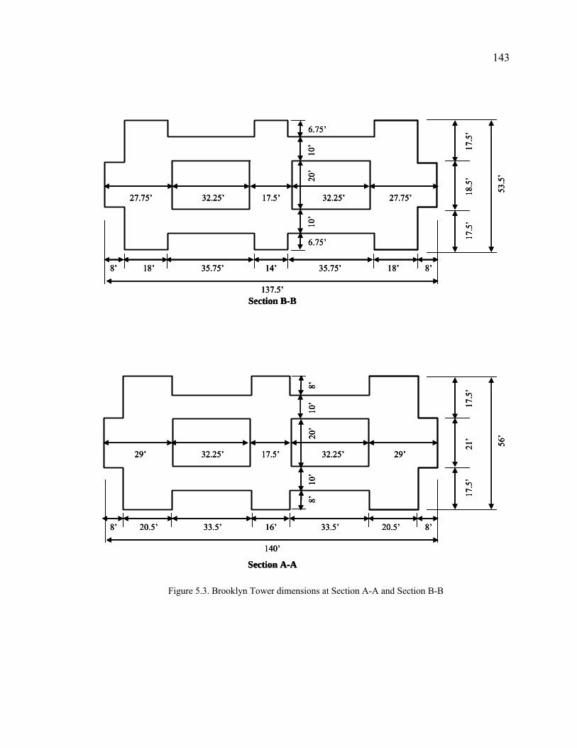
143

140’

56’

21’

17.5

’17

.5’

8’

29’32.25’17.5’

10’

20’

33.5’

8’10

’

20.5’

29’ 32.25’

8’16’33.5’20.5’8’

Section A-A

53.5

’

18.5

’17

.5’

17.5

’

27.75’32.25’17.5’27.75’ 32.25’

137.5’

35.75’ 18’ 8’14’35.75’18’8’

10’

20’

10’

6.75’

6.75’

Section B-B

140’

56’

21’

17.5

’17

.5’

8’

29’32.25’17.5’

10’

20’

33.5’

8’10

’

20.5’

29’ 32.25’

8’16’33.5’20.5’8’

Section A-A

140’

56’

21’

17.5

’17

.5’

8’

29’32.25’17.5’

10’

20’

33.5’

8’10

’

20.5’

29’ 32.25’

8’16’33.5’20.5’8’

Section A-A

53.5

’

18.5

’17

.5’

17.5

’

27.75’32.25’17.5’27.75’ 32.25’

137.5’

35.75’ 18’ 8’14’35.75’18’8’

10’

20’

10’

6.75’

6.75’

Section B-B

53.5

’

18.5

’17

.5’

17.5

’

27.75’32.25’17.5’27.75’ 32.25’

137.5’

35.75’ 18’ 8’14’35.75’18’8’

10’

20’

10’

6.75’

6.75’

Section B-B

Figure 5.3. Brooklyn Tower dimensions at Section A-A and Section B-B

144

51’

16’

17.5

’17

.5’

26.5’32.25’17.5’26.5’ 32.25’

135’

38’ 15.5’ 8’12’38’15.5’8’

10’

20’

10’

5.5’

5.5’

Section C-C

16’

14.5

’14

.5’

45’

131’

6’15.5’33.75’12’33.75’6’ 15.5’

Section D-D

51’

16’

17.5

’17

.5’

26.5’32.25’17.5’26.5’ 32.25’

135’

38’ 15.5’ 8’12’38’15.5’8’

10’

20’

10’

5.5’

5.5’

Section C-C

51’

16’

17.5

’17

.5’

26.5’32.25’17.5’26.5’ 32.25’

135’

38’ 15.5’ 8’12’38’15.5’8’

10’

20’

10’

5.5’

5.5’

Section C-C

16’

14.5

’14

.5’

45’

131’

6’15.5’33.75’12’33.75’6’ 15.5’

16’

14.5

’14

.5’

45’

131’

6’15.5’33.75’12’33.75’6’ 15.5’

Section D-D

Figure 5.4. Brooklyn Tower dimensions at Section C-C and Section D-D

145

13.5

’14

.5’

14.5

’

42.5

’

128.5’

6’13’33.75’10’33.75’6’ 13’

Section E-E

3.75’ 3.75’

16’

11’

14.5

’14

.5’

40’

126’

6’10.5’41.5’10’41.5’6’ 10.5’

Section F-F

16’

13.5

’14

.5’

14.5

’

42.5

’

128.5’

6’13’33.75’10’33.75’6’ 13’

Section E-E

3.75’ 3.75’

16’

11’

14.5

’14

.5’

40’

126’

6’10.5’41.5’10’41.5’6’ 10.5’

Section F-F

16’

11’

14.5

’14

.5’

40’

126’

6’10.5’41.5’10’41.5’6’ 10.5’

Section F-F

16’

Figure 5.5. Brooklyn Tower dimensions at Section E-E and Section F-F

146 5.3.2 Suspended Structure

The suspended structure of the Brooklyn Bridge was reconstructed in the early 1950’s

to accommodate modern traffic needs as described by Steinman (1957). The

reconstruction program included modifications to the stiffening trusses, the floor system

and the roadway deck. The suspended structure currently consists of four stiffening

trusses and a concrete deck carrying a total of six lanes of traffic. Heavy trucks are

currently prohibited from crossing the bridge. The stiffening trusses are supported by

vertical suspender cables spaced at 7.5 ft intervals. The vertical suspenders transfer the

loads from the stiffening trusses to the four main cables on the bridge. The stiffening

trusses are also partially supported near each tower by a series of diagonal stay cables.

The diagonal stays radiate down from the tops of the towers to the bottom panel points of

the stiffening trusses at intervals of 15 ft. The diagonal stays are symmetrically arranged

around each tower and consist of wire rope with diameters of 1.75 in., 1.875 in., and 2 in.

(Amman, 1947).

Steinman (1957) provides the following details about the configuration of the

stiffening trusses. The stiffening trusses in the 930-foot land spans have 125 panels and

the stiffening trusses in the river span have 107 panels between each tower and the center

of the span. The diagonal stays connect to the bottom panel points of the stiffening

trusses at alternating panels between Panel Points 7 and 55 in the land and river spans.

The stiffening trusses have hinged supports at the anchorages (Panel Point 122), and have

fixed connections at the towers. The stiffening trusses have slip joints at Panel Point 60 in

the land spans and Panel Point 104 in the river span. These slip joints which are located at

the mid-span locations of each span provide moment and axial force releases to the

147 stiffening trusses. The boundary conditions of the stiffening trusses are such that the

bridge is considered to be a five-hinged structure.

The stiffening trusses are classified as quadruple intersection Warren trusses. The

depth of each truss is 17 ft. The chord members of the trusses are constructed of 9 in.

rolled steel channel sections with webs oriented vertically. The bottom chords of the

trusses, which are subject to high compressive stresses in the regions where the diagonal

stays are located, were reinforced and stiffened with added angle sections between Panel

Points 17 and 45 in the land spans and between Panel Points 17 and 42 in the river span

during the reconstruction of the bridge. Following reconstruction of the suspended

structure, its average dead load was increased to 9,840 pounds per linear foot. The mass

of each tower is approximately 10 times greater than the mass of the portion of the

suspended spans carried by each tower.

5.3.3 Main Cables

The suspended structure is supported by four steel wire main cables each having a

diameter of 15.75 in. The total length of each main cable is 3,578.5 ft. and the weight of

each cable is 870 tons (Historic American Engineering Record). The cross sectional area

of each main cable is 144.8 sq. in. (Amman, 1947).

The main cables are supported at the tops of the towers by saddle structures on rollers

that were originally designed to permit the cables to move longitudinally with

temperature changes and unbalanced loads on the spans (Amman, 1947). The rollers

under each saddle structure have become frozen with age, and the cables may effectively

be considered to be fixed to the tops of the towers. This condition also permits the bridge

148 to act as three independent suspended spans (Amman, 1947). Past field surveys of the

bridge revealed that the deflection profile of the towers under controlled loading was

consistent with rigid body rotation about the base of the towers. This behavior has been

described as due to the elastic compressibility properties of the timber portions of the

caissons (Amman, 1947; Steinman, 1957).

5.4 Idealized Analytical Model of the Brooklyn Bridge

5.4.1 Towers

The Brooklyn and Manhattan towers were represented by identical dimensions in the

analytical model. The cross sectional dimensions used to model both towers

corresponded to those for the Brooklyn Tower. Each tower was modeled using 3D non-

prismatic beam elements with cross sectional properties coinciding with the tower at the

various levels and material properties corresponding to granite. The portion of each tower

located below the roadway level was represented by a single beam element, while the

portion above the roadway level included three separate beam elements to represent each

tower column (Figure 5.6). Rigid links were used to connect the three beam elements

together at the top of the tower and at the roadway level. The foundation conditions at

each tower were not explicitly considered in this model, and the beam elements

representing the lower portions of the towers were simply fixed in all directions at the

ground level.

Since the Manhattan Tower is founded at a deeper depth than the Brooklyn Tower,

the Young’s Modulus used for the granite material in the Manhattan Tower was reduced

149 in proportion to the ratio of the difference in foundation depths for the two towers. A

Young’s Modulus value of 7,687,000 pounds per square inches was assigned for the

granite material in the towers. The density of the granite material for the towers was

specified as 0.096 pounds (force) per cubic inch. This particular density value produced a

static dead load reaction at the tower that was equivalent to the reported self-weight of

the Brooklyn Tower. Since the Manhattan Tower has a deeper foundation depth than the

Brooklyn Tower, the Young’s Modulus specified for the granite material in the

Manhattan Tower was reduced in proportion to the difference of the foundation depths.

This made the Manhattan Tower slightly more flexible than the Brooklyn Tower.


Front ElevationIdealized Analytical Model

R.L. R.L.

R.L. R.L.


Front ElevationIdealized Analytical Model

R.L. R.L.

R.L. R.L.

Figure 5.6. Representation of towers in analytical model

150 5.4.2 Stiffening Trusses

The stiffening trusses were modeled using a single line of 3D beam elements along

the longitudinal centerline of the spans that was fixed at the towers and pinned at the

anchorage locations. This limited the modes associated with the stiffening trusses to only

vertical and lateral modes. Axial force and moment releases were provided at the

midpoint of the beam elements at the middle of each span to simulate the expansion

joints at those locations. The mass of each beam element was specified to match the

reported average dead load force per linear foot of bridge length. The section properties

specified for beam elements representing the spans initially defined according to reported

properties and were subsequently modified in an iterative fashion until the frequencies of

the first vertical and lateral modes matched those reported from the results of the ambient

vibration test performed on the spans (Kulczycki et al., 2004).

5.4.3 Main Cables

The four main cables were represented by horizontal, linear link elements connected

to the tops of the towers, and pinned at the anchorage locations. The main cables were

modeled using link elements so that their contributions to the overall dynamic response

of the structure would be included, but their dynamic responses and interactions with the

other components in the model would be suppressed. The four main cables were

represented by three physical link elements in the analytical model. The mass and

stiffness properties of the two interior main cables were combined into a single link

element located along the centerline of the bridge spans.

151 The stiffness of each spring was computed from the axial stiffness (AE/L) of the

cable for the horizontal projection of the main cable length in each span. The resulting

stiffness assigned to each link is a conservative approximation of the actual cable

stiffness; however, this is still a reasonable representation considering the objectives of

the idealized model. The mass assigned to each main cable link was computed using the

total length of each cable (3,578.5 ft) and the total weight of each cable (870 tons). The

length of the main cable assigned to each span was computed according to the

proportions of the river and land span lengths. The ratio of the length of the river span

(1,595.5 ft) to the total length of the bridge (3,535.5 ft) was multiplied by the total length

of the main cable (3,578.5 ft) to compute an estimate of the portion of the main cable in

the river span. The remaining length of the main cable was assigned equally to each land

span. These cable lengths were multiplied by the unit weight of the main cable which was

computed by dividing the total weight of each cable (870 tons) by the total length of each

cable (3,578.5 ft).

5.4.4 Stay Cables

Only one symmetric pair of diagonal stay cables at each tower was included in the

idealized analytical model. The pair of diagonal stays extending the farthest distance

from the towers in the main span and side span from each tower (the stays terminating at

Panel Point 55 in each span) was modeled using axial link elements. The stiffness

assigned to the link element was computed from the axial stiffness (AE/L) of the cable

using a stay cable diameter of 2 in. and the diagonal length from the top of the tower to

Panel Point 55 in each span. Since there are 4 separate planes of diagonal stays, the

152 computed stiffness was multiplied by 4 and applied to a single link. The mass assigned to

the axial link representing the diagonal stay in each span was estimated using the

diameter of 4 stays and a unit weight of 490 lb per cubic foot.

The inclusion of only one pair of diagonal stay cables represents a significant

simplification of reality; however, since the diagonal stay cables connect the tops of the

towers to the flexible spans, their effect on the dynamic response of the tower was

expected to be minimal. The vertical suspender cables were not represented in the

idealized model since they are not physically connected to the towers and their dynamic

responses would add unnecessary complexity to the analysis results.

5.5 Results

Several views of the idealized analytical model are shown in Figure 5.7. The different

model cases analyzed are shown with the principal bridge components included for each

case in Figure 5.8. The natural frequencies for the first two longitudinal, torsional, and

lateral modes of the Brooklyn Tower were extracted from each analysis case. The

analytical natural frequencies are summarized in Table 5.1.

The frequencies associated with each Brooklyn Tower mode change very little

between the different model cases. The addition of the main cables leads to an increase in

the frequency of the first longitudinal mode of the Brooklyn Tower. This indicates that

the main cables do stiffen the tower in the longitudinal direction; however, the do not add

enough stiffness to change the first longitudinal mode shape from that associated with a

simple cantilever beam to that corresponding to a propped cantilever beam. Thus, even

though the main cables were modeled using very conservative estimates of their true

153 stiffness, they do not add enough restraint to the tops of the tower to fundamentally

change the character of the first longitudinal mode shape. This tends to confirm the

observation that the Brooklyn Bridge behaves as a weakly-coupled dynamic system.

The addition of the stay cables does not significantly influence the natural frequencies

of the Brooklyn Tower. This may be observed by comparing the results from the Towers-

Spans and the Towers-Spans-Stays cases. This is a reasonable result in that the stay

cables radiate from a single location at the top of the tower and terminate at various

points along the very flexible span. As a result, the stay cables do not effectively brace

the top of the tower and change its fundamental dynamic response. The stay cables

essentially ride along with the response of the tower since they are connected to a flexible

support (the spans). The stay cables do add mass to the model, and including additional

stays may change the natural frequencies somewhat due to added mass, however, they do

not restrain the dynamic motion of the towers.

Table 5.1. Brooklyn Tower modes for different model cases

Natural Frequency (Hz)

Description

Free Standing

Towers Towers-

Cables

Towers-Cables-

Spans Towers-

Spans

Towers-Spans-

Stays

Towers-Cables-Spans-

Stays Mode 1 1st Longitudinal 1.799 1.919 1.964 1.857 1.872 1.976 Mode 2 1st Lateral 2.896 2.793 2.791 2.894 2.893 2.790 Mode 3 1st Torsional 4.046 4.015 4.032 4.063 4.063 4.032 Mode 4 2nd Longitudinal 5.096 5.014 4.981 5.061 5.062 4.983 Mode 5 2nd Lateral 7.196 7.171 7.089 7.114 7.113 7.088 Mode 6 2nd Torsional 8.047 7.933 7.944 8.056 8.056 7.943

154

Main Cables (links)

Diagonal Stays (links)

Stiffening Trusses (beam element)

Towers(beam elements)

Free-standing Towers

Towers, Main Cables, Spans & Stays

Deck Level

Top

Base

Main Cables (links)

Diagonal Stays (links)

Stiffening Trusses (beam element)

Towers(beam elements)

Free-standing Towers

Towers, Main Cables, Spans & Stays

Deck Level

Top

Base

Figure 5.7. Representation of different bridge components in the idealized model


Towers – Main Cables

Towers - Main Cables - Spans

Towers – Spans

Towers – Spans – Stay Cables

Towers – Main Cables – Spans – Stay Cables


Towers – Main Cables

Towers - Main Cables - Spans

Towers – Spans

Towers – Spans – Stay Cables

Towers – Main Cables – Spans – Stay Cables

Figure 5.8. Principal bridge components included in different analytical model cases

155 The order of the Brooklyn Tower modes also does not change from the free-standing

towers case and the cases where other components of the bridge are included. The

difference in stiffness assigned to the Brooklyn Tower and Manhattan Tower to account

for their different foundation depths results in the modes of each tower being independent

of each other. In other words, there are 6 fundamental modes associated with the

Manhattan Tower that occur at different frequencies than the same 6 fundamental modes

for the Brooklyn Tower.

The mode shapes for the first six modes of the Brooklyn Tower from the free-

standing towers model case are shown in Figure 5.9. The Manhattan Tower is essentially

stationary at each of these modes. The first 6 modes of the Brooklyn Tower for the model

case which included representations of all of the bridge components are shown in Figure

5.10 and Figure 5.11. These illustrate a similar behavior in that the Manhattan Tower is

essentially stationary for the modes associated with the Brooklyn Tower. The separation

of the modes for the different components is consistent with the behavior expected for a

weakly-coupled dynamic system.

The mode shapes associated with each natural frequency of the Brooklyn Tower were

fairly consistent for each of the model cases analyzed. The first two longitudinal, lateral,

and torsional mode shapes computed from each model case are shown in Figure 5.12,

Figure 5.13, and Figure 5.14, respectively. The mode shapes shown in these figures are

unit normalized to permit them to be compared on a consistent basis. It may be observed

from the mode shapes shown in these figures that there are slight differences in the

amplitudes of the mode shapes at some degrees of freedom for some of the model cases.

156 These differences are generally more pronounced in the 2nd longitudinal, torsional, and

lateral mode shapes than the 1st longitudinal, torsional, and lateral mode shapes.

The modal amplitudes are different for the model cases that included representations

of the main cables and those which did not. In other words, the amplitudes of the mode

shapes are slightly different for the model cases which included the main cables and those

which did not. The tops of the towers are more flexible in the cases which did not include

the main cables, and the resulting normalized mode shape amplitudes for these models

are slightly different from the cases where the main cables were included. This also

indicates that the main cables stiffen the tops of the towers in both the longitudinal and

lateral directions. The stiffness provided by the main cables effectively changes the

amplitude of the top of the tower in each mode; however, the change is not sufficient to

fundamentally alter the character of the mode shapes.

Another observation that may be made from the results of the idealized analytical

model cases relates to the coupled motions of the different bridge components for modes

associated with one particular component of the weakly-coupled system. There is motion

associated with each component of the bridge at every natural frequency; however, the

nature of the motion associated with each bridge component at these natural frequencies

is clearly different. For example, the spans are observed to vibrate at the tower natural

frequencies; however, the nature of these oscillations appears to be consistent with local

or higher order modes of the spans. There are some instances where the motion of the

span at a tower mode frequency has a shape that is similar to one of the fundamental

modes of the span; however, the nodal points in the span responses are observed to

exhibit the traveling wave behavior that is associated with complex modes.

157

Brooklyn Tower 1st Longitudinal

f = 1.799 HzBT

BT

BT

MT

MT

MT

Brooklyn Tower 1st Lateral

f = 2.896 Hz

Brooklyn Tower 1st Torsional

f = 4.046 Hz

BT

BT

BT

MT

MT

MT

Brooklyn Tower 2nd Longitudinal

f = 5.096 Hz

Brooklyn Tower 2nd Lateral

f = 7.196 Hz

Brooklyn Tower 2nd Torsional

f = 8.047 Hz


f = 1.799 HzBT

BT

BT

MT

MT

MT


f = 2.896 Hz


f = 4.046 Hz

BT

BT

BT

MT

MT

MT


f = 5.096 Hz


f = 7.196 Hz

Brooklyn Tower 2nd Torsional

f = 8.047 Hz

Figure 5.9. First six modes of the Brooklyn Tower from the free-standing towers analysis case

The towers are also observed to vibrate in their fundamental mode shapes at some of

the natural frequencies associated with the spans, but the modal displacements in these

cases are significantly less than those which occur at the frequencies associated with the

modes of each tower. This observation is reflected by the modal displacements shown for

the Brooklyn Tower from the towers-main cables-stay cables-spans analysis case shown

in Figure 5.15. Unit normalized longitudinal modal displacements of the tower are shown

in the figure at frequencies corresponding to vertical modes of the spans (the leftmost

graph) and for frequencies corresponding to pure tower longitudinal modes (the central

158 graph). The unit normalized shapes for the tower are clearly very comparable for modes

associated with the vertical modes of the spans and for the first longitudinal mode of the

tower. When the absolute (non-normalized) modal deformations associated with the span

and tower frequencies are compared (the rightmost graph), it is clear that the longitudinal

modal deformations associated with the tower modes are at least an order of magnitude

larger than those associated with the vertical modes of the spans. Therefore, although the

modal deformations of the tower have similar shapes for both span and tower modes, the

modal deformations of the tower at the tower modes clearly represent the most critical

case for design and analysis. Furthermore, the mode shapes and frequencies

corresponding to the tower modes should be the principal focus of the experimental

identification and subsequent model calibration, particularly for seismic retrofit

considerations.

159

BT

BT

BT


f = 1.976 Hz


f = 2.790 Hz


f = 4.032 Hz

BT

BT

BT

MT

MT

MT

Figure 5.10. First longitudinal, lateral and torsional modes of the Brooklyn Tower

160

BT

BT

BT


f = 4.983 Hz


f = 7.088 Hz


f = 7.943 Hz

MT

MT

MT

BT

BT

BT

Figure 5.11. Second longitudinal, lateral and torsional modes of the Brooklyn Tower

161

0

50

100

150

200

250

0.0 0.2 0.4 0.6 0.8 1.0

Free Stand Towers

Towers Cables

Towers Cables Spans

Towers Spans

Towers Spans Stays

Towers Cables Spans Stays

0

50

100

150

200

250

-1.0 -0.5 0.0 0.5 1.0

Free Stand Towers

Towers Cables

Towers Cables Spans

Towers Spans

Towers Spans Stays



1st Longitudinal Mode 2nd Longitudinal Mode

Hei

ght A

bove

Tow

er B

ase

(ft)

0

50

100

150

200

250

0.0 0.2 0.4 0.6 0.8 1.0

Free Stand Towers

Towers Cables

Towers Cables Spans

Towers Spans

Towers Spans Stays


0

50

100

150

200

250

-1.0 -0.5 0.0 0.5 1.0

Free Stand Towers

Towers Cables

Towers Cables Spans

Towers Spans

Towers Spans Stays




Hei

ght A

bove

Tow

er B

ase

(ft)

0

50

100

150

200

250

0.0 0.2 0.4 0.6 0.8 1.0

Free Stand Towers

Towers Cables

Towers Cables Spans

Towers Spans

Towers Spans Stays


0

50

100

150

200

250

-1.0 -0.5 0.0 0.5 1.0

Free Stand Towers

Towers Cables

Towers Cables Spans

Towers Spans

Towers Spans Stays




Hei

ght A

bove

Tow

er B

ase

(ft)

Figure 5.12. 1st and 2nd unit normalized longitudinal mode shapes for different model cases

162

0

50

100

150

200

250

0.0 0.2 0.4 0.6 0.8 1.0

Free Stand Towers

Towers Cables

Towers Cables Spans

Towers Spans

Towers Spans Stays


0

50

100

150

200

250

-1.0 -0.5 0.0 0.5 1.0

Free Stand Towers

Towers Cables

Towers Cables Spans

Towers Spans

Towers Spans Stays


1st Lateral Mode 2nd Lateral Mode


Hei

ght A

bove

Tow

er B

ase

(ft)

0

50

100

150

200

250

0.0 0.2 0.4 0.6 0.8 1.0

Free Stand Towers

Towers Cables

Towers Cables Spans

Towers Spans

Towers Spans Stays


0

50

100

150

200

250

-1.0 -0.5 0.0 0.5 1.0

Free Stand Towers

Towers Cables

Towers Cables Spans

Towers Spans

Towers Spans Stays


1st Lateral Mode 2nd Lateral Mode


Hei

ght A

bove

Tow

er B

ase

(ft)

Figure 5.13. 1st and 2nd unit normalized lateral mode shapes for different model cases

163

0

50

100

150

200

250

0.0 0.5 1.0 1.5

Free Stand Towers

Towers Cables

Towers Cables Spans

Towers Spans

Towers Spans Stays


0

50

100

150

200

250

-1.0 -0.5 0.0 0.5 1.0

Free Stand Towers

Towers Cables

Towers Cables Spans

Towers Spans

Towers Spans Stays


Hei

ght A

bove

Tow

er B

ase

(ft)


1st Torsional Mode 2nd Torsional Mode

0

50

100

150

200

250

0.0 0.5 1.0 1.5

Free Stand Towers

Towers Cables

Towers Cables Spans

Towers Spans

Towers Spans Stays


0

50

100

150

200

250

-1.0 -0.5 0.0 0.5 1.0

Free Stand Towers

Towers Cables

Towers Cables Spans

Towers Spans

Towers Spans Stays


Hei

ght A

bove

Tow

er B

ase

(ft)


1st Torsional Mode 2nd Torsional Mode

Figure 5.14. 1st and 2nd unit normalized torsional mode shapes for different model cases

0.0

10.0

20.0

30.0

40.0

50.0

60.0

70.0

80.0

-2.0E-02 -1.0E-02 0.0E+00 1.0E-02 2.0E-02 3.0E-02

0.305

0.482

0.535

1.387

1.570

1.976

4.983

0.0

10.0

20.0

30.0

40.0

50.0

60.0

70.0

80.0

-1.0 -0.5 0.0 0.5 1.0

Amplitude

1.976

4.983

0.0

10.0

20.0

30.0

40.0

50.0

60.0

70.0

80.0

-1.0 -0.5 0.0 0.5 1.0

0.305

0.482

0.535

1.387

1.570

Hei

ght A

bove

Tow

er B

ase

(m)

Hei

ght A

bove

Tow

er B

ase

(m)

Unit Normalized Modal Amplitude

Absolute Modal Amplitude


Main & Side Span Vertical Modes

Tower Longitudinal Modes Tower Longitudinal & Span Vertical Modes

0.0

10.0

20.0

30.0

40.0

50.0

60.0

70.0

80.0

-2.0E-02 -1.0E-02 0.0E+00 1.0E-02 2.0E-02 3.0E-02

0.305

0.482

0.535

1.387

1.570

1.976

4.983

0.0

10.0

20.0

30.0

40.0

50.0

60.0

70.0

80.0

-1.0 -0.5 0.0 0.5 1.0

Amplitude

1.976

4.983

0.0

10.0

20.0

30.0

40.0

50.0

60.0

70.0

80.0

-1.0 -0.5 0.0 0.5 1.0

0.305

0.482

0.535

1.387

1.570

Hei

ght A

bove

Tow

er B

ase

(m)

Hei

ght A

bove

Tow

er B

ase

(m)


Absolute Modal Amplitude


Main & Side Span Vertical Modes

Tower Longitudinal Modes Tower Longitudinal & Span Vertical Modes

Figure 5.15. Longitudinal modal displacements of Brooklyn Tower at discrete span and tower modes

164 5.6 Discussion

The observations from the analyses of the idealized models that are most relevant to

the interpretation of the experimental measurements may be summarized as follows:

1. The analyses of the idealized model indicate that there are interactions between the

towers and the spans at every frequency, and that the towers respond in the

longitudinal, torsional and lateral response directions at every frequency. The nature

of these interactions and the tower responses in each direction is very different at the

frequencies that are primarily associated with the towers and those which are

associated with the span modes.

2. There were no frequencies identified where the responses of both the towers and

spans are consistent with simultaneous resonance of both components. Furthermore,

there were no natural frequencies identified for the towers where there is an

indication that the tower simultaneously resonates in more than one of its primary

response directions. This indicates that there should be no coupled tower-span modes

(a global structure modes) or coupled tower modes in which the tower resonates in

more than one direction at the same natural frequency. Interactions between the

towers and spans exist at all frequencies just as the tower responds in all directions at

all frequencies, however, these interactions are more consistent with the coupled

motions that would occur if an excitation was applied between a tower mode and a

span mode, instead of the tower mode and span mode being collocated at the same

frequency.

3. The modes associated with the maximum tower response are distinct from modes

associated with the maximum response of the other bridge components. These distinct

165 tower modes can be identified in the results from each model case as the idealized

model progresses from the free-standing towers representation to the final case that

included effects of the towers, spans, main cables and stay cables. The natural

frequencies associated with the tower modes change as the mass and stiffness effects

of the additional bridge components are included, but the corresponding tower mode

shapes remain essentially the same. This indicates that the Brooklyn Bridge may

indeed be considered to behave as a weakly-coupled dynamic system.

4. The absolute modal displacements of the towers at the distinct tower modes are most

significant in only direction; therefore, the tower modes may be characterized as pure

longitudinal, pure torsional, or pure lateral modes

5. The towers do participate in varying degrees in all directions with the modes

associated with other bridge components (for example the span modes), but the

absolute modal displacements of the towers in any direction at these frequencies are

insignificant when compared with the modal displacements associated with the pure

tower modes

6. There are likely to be 6 distinct natural frequencies identified for the Brooklyn Tower

in the frequency range of 0 to 10 Hz. The natural frequencies identified for the

Brooklyn Tower from ambient vibration testing may have values that are quite

different from those in the idealized model as this represents a very approximate

representation of the bridge; however, the order of the experimentally identified

modes should follow the trend observed in this model.

7. The idealized model indicates that the dynamic behavior of the cable-supported

structure is indeed complex. It also suggests that there are several different levels of

166 response possible for the towers and spans depending on the nature of the force that is

applied to the structure. The different responses possible for each component for a

given excitation may be exemplified by the following load case and responses:

• Case 1: A static load is applied to the midspan location of the main span in the

vertical direction with a magnitude F. Due to the physical connections between

the towers and spans, the span will undergo a static vertical deflection of ∆V, and

the towers will experience a static longitudinal deflection of ΔL. The longitudinal

deflected shape of the tower will not be the same as the modal configuration

associated with first longitudinal tower mode, although it may be similar to it.

• Case 2: A time varying vertical load is applied to the mdispan location of the

main span with a magnitude F(t) and a frequency that is not at or close to the first

natural frequency associated with the span (vertical) or the tower (longitudinal).

The vertical deflection of the span will also vary with time, but the maximum

value of the vertical deflection will be less than or equal to the maximum static

deflection from Case 1. The longitudinal deflection of the towers will also vary

with time, but the maximum value will be less than or equal to the static

deflection from Case 1. The longitudinal deflected shape of the tower will not be

the same as the modal configuration associated with first longitudinal tower

mode, although it may be similar to it.

• Case 3: A time varying vertical load is applied to the midspan of the main span

with a magnitude F(t) and a frequency that is very close to or at the first vertical

natural frequency of the span, but not close to or at the first natural frequency of

the tower. The vertical deflection response of the main span will experience

167 dynamic amplification (resonance), and its maximum value will be greater than its

maximum value in Case 1 or Case 2. The longitudinal deflections of the towers

will vary with time, and the magnitude of the longitudinal deflection will be

greater than the maximum tower deflection in Case 1 or Case 2. The amplification

of the tower response in this case is not a related to the mass and stiffness

characteristics of the towers; it is the result of the amplified vertical deflection

that occurs for the spans. The longitudinal deflected shape of the tower will not be

the same as the modal configuration associated with first longitudinal tower

mode, although it may be similar to it.


with a magnitude F(t) and at a frequency that is very close to or at the first

longitudinal natural frequency of the tower, but not close to or at the first vertical

natural frequency of the span. The vertical deflection of the span will vary with

time and its maximum value will be larger than in Case 1 or Case 2, but less than

its maximum value in Case 3. The longitudinal deflection response of the tower

will experience dynamic amplification (resonance), and its maximum value will

be larger than its maximum value in Case 1, Case 2 or Case 3. The longitudinal

deflected shape of the tower be consistent with the modal configuration associated

with first longitudinal tower mode. The amplification of the span response in this

case is not related to the mass and stiffness characteristics of the main span; it is

the result of the amplified tower deflections.


with a magnitude F(t) and at a frequency that is very close to or at the first

168 vertical natural frequency of the span and very close to or at the first longitudinal

natural frequency of the tower. The span and tower modes are coupled (global

structural mode) in this case. The vertical deflection of the span will vary with

time and experience dynamic amplification (resonance). Its maximum value will

be larger than in Case 1, Case 2, Case 3 or Case 4 due to its own amplified motion

and the dynamic amplification of the tower responses. The longitudinal deflection

of the tower will also vary with time and will experience dynamic amplification

(resonance). Its maximum value will be larger than in Case 1, Case, 2, Case 3, or

Case 4 due to its own amplified response and the amplified response of the main

span. This case will produce the maximum responses for both the span and the

tower, but this case depends on the existence of a coupled tower-span mode.

8. The different response cases will all create peaks in the output spectra for the towers

in the longitudinal response direction. The challenge is to identify the peaks

associated with the maximum response of the tower (Case 4 or Case 5) from the

peaks that will be associated with the other cases. These will represent the critical and

most meaningful tower modes with respect to validating finite element models of the

bridge, or for designing a seismic retrofit.

Experimental Characterization of Towers in Cable-Supported Bridges

by Ambient Vibration Testing

Volume 2

A Thesis

Submitted to the Faculty

of

Drexel University

by

Kirk Alexander Grimmelsman

in partial fulfillment of the

requirements for the degree

of

Doctor of Philosophy

December 2006

169 CHAPTER 6: MODAL IDENTIFICATION OF A CANTILEVER BEAM

6.1 Introduction

The ambient vibration testing technique requires that a number of assumptions are

made with respect to the character of the ambient dynamic excitation in addition to

assumptions related to the structure itself. The most fundamental of these assumptions are

that the ambient dynamic excitation is stationary with zero mean, it is ergodic, and it has

broadband Gaussian or white noise characteristics for the frequency band of interest. It is

generally understood that the ambient excitation environment for a real structure will

rarely conform exactly to these ideal assumptions; however, the degree to which this

nonconformance affects the modal identification process has not been well-established.

This is most probably due to the fact that it is very difficult to directly measure and

completely characterize the nature of ambient dynamic excitation for an in-service

structure. It will be shown in a subsequent section of this chapter that character of the

ambient dynamic excitation for cable supported bridges such as suspension bridges can

be very complex. Furthermore, the character of the ambient excitation may be quite

different for the various subcomponents of these bridges. The effects of possible

variations in the ambient dynamic excitation from its assumed nature on the reliability of

the identified modal parameters is a particularly relevant issue for ambient vibration tests

of cable-supported bridges and their subcomponents; however, these effects have not

been adequately identified and evaluated in the available literature.

The effectiveness of different modal identification methods in cases where the

ambient dynamic excitation is complex or varies from its assumed nature is also not well-

170 established. A number of researchers have compared the attributes and effectiveness of

different modal identification algorithms for simulated ambient vibration measurements

or for ambient measurement data from different constructed systems including bridges.

Peeters (2000) evaluated several different modal identification methods for simulated

ambient response data with different levels of superimposed random noise, and for

ambient vibration measurements from the Z-24 Bridge in Switzerland. The use of

simulated ambient measurement data is a valid approach for evaluating different modal

identification methods; however, it is difficult to realistically simulate the various sources

of uncertainty and complexity in the measurements that are frequently encountered

during tests on real structures. Low level responses buried in various degrees of random

noise represent one of many possible sources of uncertainty in the modal identification of

ambient vibration measurements.

Peeters and Ventura (2003) subsequently described and compared the results of

different modal identification methods used by different research teams for forced-

vibration, free vibration, and ambient vibration data from the Z-24 Bridge. Since the Z-24

Bridge was a concrete box girder bridge, the results of these comparative evaluations may

not necessarily be valid for other types of bridges or the subcomponents of some types of

bridges. He et al. (2006) recently compared different modal parameter identification

methods for free and ambient vibration measurements from a suspension bridge. The

unmeasured dynamic excitation consisted of vertical pulses due to a heavy truck driving

over small ramps for a portion of the span followed by normal driving across the

remainder of the bridge. The vertical and torsional responses of the suspended portion of

the structure (the spans) were identified and compared using different modal

171 identification methods. Although the character of the dynamic excitation was somewhat

controlled and the resulting excitation has a complex nature, it does not represent a

realistic simulation of the typical nature of ambient dynamic excitation for the suspended

spans of a suspension bridge. Furthermore, since only the vertical (and torsional)

responses of the spans are identified for excitation that was predominately in vertical

direction, the capabilities of the different identification methods are not evaluated for

response directions in which the excitation and the corresponding measurements may not

be as clear. The evaluation also does not consider the effects of dynamic interactions

between the towers and the flexible spans since the tower responses were not measured or

characterized. Therefore, the findings from this comparative evaluation may only be

applicable for a specific portion of a suspension bridge (the flexible spans) and for the

ambient vibration responses in a particular direction. It should also be noted that the

uncertainty associated with the modal parameter identification of suspension bridges is

generally the smallest for the vertical and torsional responses under ambient vibration

excitation due to traffic.

There is merit in comparing and evaluating different modal parameter identification

methods ambient vibration responses from in-service structures since the measurements

will automatically reflect the various experimental errors, dynamic interactions of

different structural subcomponents, and the true nature of the ambient dynamic

excitation. Ambient vibration measurements from an in-service structure will permit the

effectiveness of different identification methods to be evaluated on a consistent basis (for

the particular structural configuration and ambient dynamic excitation characteristics

considered) under realistic conditions; however, because the ambient dynamic excitation

172 can not be controlled or measured, the possible characteristics of the ambient dynamic

excitation on the resulting identification are not explicitly considered in the evaluation

process. The different methods are simply applied to the measured responses and their

results are compared. It can be very difficult to reliably identify the expected dynamic

behavior of some complicated structures, so establishing the exact solution for a structure

to compare with the experimental results may be a significant challenge. Furthermore,

since the nature of the ambient dynamic excitation and will be different for different

types of structures and for the different subcomponents of a single structure, the results of

such evaluations may be limited to structures that have similar structural behavior

characteristics and are exposed to ambient dynamic excitation with similar characteristics

to those considered in the comparative evaluation.

It follows that the character of the ambient dynamic excitation is an important

parameter that should be considered when evaluating and comparing the utility of

different modal parameter identification methods and for understanding the reliability of

the identified dynamic properties. In order to consider the characteristics of the ambient

dynamic excitation, it needs to be characterized and controlled. This ambient excitation

cannot be controlled or practically characterized by measurements for most in-service

structures, but there are two alternative approaches which may be employed to conduct

such an evaluation.

The first approach may be to utilize simulated response or excitation signals for

conducting the evaluation. Measurement signals with various levels of complexity or

uncertainty can be mathematically generated and analyzed directly, or simulated

excitation signals with different characteristics may be fed into numerical or analytical

173 models of a structure to generate corresponding responses for subsequent analysis. An

advantage of this approach is that the signals may be precisely defined and many possible

permutations of ambient excitation may be quickly generated and evaluated. In addition,

if the simulated excitation is used in conjunction with a numerical or analytical model of

a structure, the effects of different structural configurations and any dynamic interactions

between its subcomponents may be included in the evaluation. A disadvantage of this

approach is that it may be difficult to realistically and reliably identify, characterize and

duplicate the various experimental, structural and excitation related sources of

uncertainty that are present during ambient vibration tests of in-service structures.

A second possible approach is to utilize a physical model in the laboratory to evaluate

the influence of the character of the ambient dynamic excitation. The physical model in

this case may represent a scale model of an actual structure, or it may simply represent a

structure that is to be characterized by ambient vibration testing. Various characteristics

of ambient dynamic excitation may be simulated and applied to the physical model using

small scale shakers or other dynamic excitation devices. Although the characteristics of

the dynamic excitation applied to the model are controlled, this excitation is treated as

though it is unmeasured for identifying the dynamic properties. One advantage of this

approach is that since real excitation and measurements are used in conjunction with a

physical structure, it is possible to incorporate realistic sources of complexity and

uncertainty associated with the experiment, the excitation, and the dynamic response of

the structure. The main disadvantage of this approach is that more time is required to

evaluate a particular excitation case, and multiple excitation devices may be required to

generate complex dynamic excitation.

174 This chapter describes the identification of a simple cantilever beam used as a

physical laboratory model by ambient vibration testing methods. The beam was subjected

to various cases of dynamic excitation to evaluate the effects of deviations from the

assumed character of ambient dynamic excitation. The measurement data was processed

using several common modal identification methods that have been used with bridges to

compare and evaluate their effectiveness for different cases of ambient dynamic

excitation.

6.2 Scope

A simple cantilever beam was utilized as a physical model in the laboratory to

evaluate the effects of the character of the ambient dynamic excitation on the identified

dynamic properties of the beam, and to compare the results obtained using different

modal identification methods. The theoretical solution for the dynamic properties

(frequencies and mode shapes) of the beam was computed to establish the expected

dynamic behavior (frequency range, modal order, mode shapes, etc.).

A number of different excitation cases were defined based on a qualitative

characterization of the ambient dynamic excitation for cable supported bridges. Of

particular interest is the character of the ambient dynamic excitation for the tower of a

suspension bridge. Several ambient excitation cases were designed based on the

qualitative characterization of the ambient dynamic excitation for the towers and pylons

in cable supported bridges, and applied to the cantilever beam in the laboratory. The

excitation cases developed were intended to simulate two primary characteristics relevant

to the ambient excitation of the towers or pylons in cable-supported bridges. The first

175 characteristic considered was ambient dynamic excitation with different frequency

bandwidths that represented various fractions of the full frequency bandwidth of interest

for the structure under test. The second characteristic considered was the presence of

harmonics in the ambient dynamic excitation spectrum. The applied dynamic excitation

was also spatially restricted in this study as is often the case for the traffic related

dynamic excitation or ground motions that are transmitted to the towers and pylons of

cable-supported bridges.

The measurement data was processed to extract the frequencies and mode shapes for

the cantilever beam using several different modal identification methods commonly used

in ambient vibration experiments of in-service bridges, including cable-supported

structures. These methods included peak picking (PP), the polyreference time domain

(PTD) method, the complex mode indicator function (CMIF) method, and finally the

stochastic subspace identification (SSI) method. Because the damping ratios identified by

ambient vibration testing have been shown to be very sensitive to the excitation level and

are associated with a high degree of uncertainty (Abdel-Ghaffar and Housner, 1978;

Brownjohn, 1994; Doebling et al., 1997; Kareem and Gurley, 1999; Nagayama et al.,

2005), they were not considered in conjunction with these tests. A broad-band Gaussian

excitation case was applied to the beam to serve as a modal identification benchmark for

comparing the different identification methods. Although the character of the dynamic

excitation was controlled in each case, it was treated as unmeasured ambient excitation

for the purpose of identifying the modal properties of the beam.

176 6.3 Description of the Test Specimen

The laboratory test specimen used for this study was a thin-walled rectangular steel

tube section with external dimensions of 3 inches by 1.5 inches. The wall thickness of the

tube section was 1/8 inches. The test specimen was clamped near one end to a pedestal

support to form a cantilever beam with an unsupported length of 117.5 inches as shown

in Figure 6.1 and Figure 6.2. Furthermore, the beam was oriented on the pedestal support

so that it would bend under its own weight about its weak-axis direction. The relevant

material and section properties for the cantilever beam are summarized in Table 6.1.

Figure 6.1. Cantilever beam specimen in the laboratory

177

Figure 6.2. Clamped support condition for the cantilever beam

Table 6.1. Mechanical and material properties of the cantilever beam

Property Value Units Young’ Modulus, E 29x106 lb-f/in2 Density, ρ 0.284 lb-f/in3 Cross Sectional Area, A 0.956 in2 Mass per Unit Length 7.016x10-4 lb-m/in Moment of Inertia, I 0.355 in4 Span Length, L 117.5 in

178 6.3.1 Theoretical Dynamic Properties of the Cantilever Beam

The theoretical dynamic properties of a structure may be quite different from the

actual properties of the structure as determined through testing. The first five theoretical

frequencies and mode shapes of the beam were calculated to guide the design of the

experimental program and to serve as a consistent baseline for comparing the results of

the different experimental cases. Some basic assumptions were made regarding the beam

section prior to formulating the theoretical solution. First, it was assumed that the

dynamics of the cantilever beam could be more accurately described by a system with

distributed mass and stiffness since the masses of the installed accelerometers were

negligible relative to the mass per unit length of the steel tube section. Second, because

the ratio of the beam depth to span length was very small, it was assumed that the effects

of shear deformation and rotational inertia could be excluded from the analysis. Finally,

the damping was assumed to be small enough that the equation of undamped motion

would adequately describe the dynamics of the cantilever beam. .

Taking advantage of the above assumptions, the theoretical solution for the free

transverse vibration of a beam with distributed mass and stiffness may be determined by

following the partial differential equation derivations outlined by Chopra (1995). For the

special case of a beam with uniform mass and stiffness, the free vibration can be

described by the following characteristic equation:

0)()( 44

4

=− xdx

xd φβφ (6.1)

where

179

EIm2

4 ωβ = (6.2)

and m = mass per unit length, ω = natural frequency, E = Young’s Modulus, and I =

moment of inertia. The general solution of Eq. (6.1) is:

xCxCxCxCx ββββφ coshsinhcossin)( 4321 +++= (6.3)

which contains four unknown constants and the eigenvalue parameter β. For the case

of a cantilever beam, the displacement and slope at the clamped end (x = 0) are zero and

the moment and shear at the free end (x = L) are zero. These boundary conditions may be

expressed as follows:

⎪⎪⎭

⎪⎪⎬

⎫

=

=

0)(

0)(

dxxd

x

φ

φ at x = 0 (6.4)

⎪⎪

⎭

⎪⎪

⎬

⎫

=

=

0)(

0)(

3

3

2

2

dxxdEI

dxxdEI

φ

φ

at x = L (6.5)

Using these expressions for the boundary conditions with Eq. (6.3) gives the

following:

24 CC −= (6.6)

13 CC −= (6.7)

180 0)cosh(cos)sinh(sin 21 =+++ LLCLLC ββββ (6.8)

0)sinhsin()cosh(cos 21 =+−++ LLCLLC ββββ (6.9)

Eqs. (6.8) and (6.9) can be combined in matrix form to give:

⎥⎦

⎤⎢⎣

⎡=⎥

⎦

⎤⎢⎣

⎡⎥⎦

⎤⎢⎣

⎡+−+

++00

sinhsincoshcoscoshcossinhsin

2

1

CC

LLLLLLLL

ββββββββ

(6.10)

For a non-trivial solution, the determinate of the coefficient matrix must equal zero.

This leads to the following equation for frequency:

0coshcos1 =+ LL ββ (6.11)

Eq. (6.11) may be solved numerically to obtain the following solutions for the term βL:

996.10 and,8548.7,6941.4,8751.1=Lnβ (6.12)

for n = 1, 2, 3, and 4. For values of n that are larger than 4, the term β L is given by the

following expression:

2)12( πβ −≈ nLn (6.13)

The first five natural frequencies of the cantilever used in this study will be

determined for comparison with the experimental results. Using Eqs. (6.2), (6.12), and

(6.13), the following expressions may be developed for the first five natural frequencies

of the cantilever beam:

mEI

L21516.3

=ω (6.14)

181

mEI

L2203.22

=ω (6.15)

mEI

L2370.61

=ω (6.16)

mEI

L249.120

=ω (6.17)

mEI

L2586.199

=ω (6.18)

The mode shape corresponding to each value of βnL is derived by expressing C2 in

terms of C1 from Eq. (6.8) and substituting the result into Eq. (6.3). After simplifying, the

following expression is obtained:

( )⎥⎦

⎤⎢⎣

⎡−

++

−−= xxLLLL

xxCx nnnn

nnnnn ββ

ββββ

ββφ sinsinhsinsinhcoscosh

coscosh)( 1 (6.19)

The first five natural frequencies of the cantilever beam test specimen computed

using the equations above are summarized in Table 6.2. The mode shapes corresponding

to the first five natural frequencies of the cantilever beam are summarized in Figure 6.3.

The computed mode shape coordinates were unit normalized for subsequent comparisons

with the experimental results. The unit normalized mode shape coordinates for each

mode are also provided in Table 6.2.

182 Table 6.2. Theoretical natural frequencies and mode shape coordinates for the cantilever beam

Unit Normalized Mode Shape Coordinate at Measurement Degree of Freedom

Mode Frequency

(rad/sec) Frequency

(Hz) 1 2 3 4 5 6 1 30.850 4.910 0 -0.064 -0.230 -0.461 -0.725 -1

2 193.333 30.770 0 0.301 0.683 0.589 -0.070 -1

3 541.341 86.157 0 0.604 0.526 -0.474 -0.395 1

4 1060.9 168.846 0 0.753 -0.316 -0.326 0.643 -1

5 1753.6 279.091 0 0.660 -0.697 0.700 -0.600 1

φ1 (x)

φ2(x)

φ3(x)

φ4(x)

φ5(x)

x

φL = 117.5 in

φ1 (x)

φ2(x)

φ3(x)

φ4(x)

φ5(x)

φ1 (x)

φ2(x)

φ3(x)

φ4(x)

φ5(x)

x

φL = 117.5 in

Figure 6.3. Theoretical unit normalized mode shapes for the cantilever beam

183 6.4 Ambient Dynamic Excitation Characteristics for Cable-Supported Bridges

Although it is nearly impossible to objectively characterize the ambient dynamic

excitation for most structures directly by measurements, it may be possible to

qualitatively describe its characteristics. Cable supported bridges represent a special class

of bridge structures consisting of very flexible spans connected to relatively stiffer tower

or pylon structures. It will be shown in the following that the structural configuration for

these bridges coupled with ambient dynamic excitation that is predominately due to

traffic may lead to complex ambient dynamic excitation for the various subcomponents

of the bridge that may diverge quite drastically from the assumed character for ambient

dynamic excitation in ambient vibration testing applications.

The logical starting point for a qualitative characterization of the ambient dynamic

excitation for these structures would be a classification of the possible sources of ambient

dynamic excitation for in-service bridges. The ambient dynamic excitation for most

constructed systems may be classified as either due to direct or indirect sources as shown

in Figure 6.4. A direct source of ambient excitation may be defined as external dynamic

excitation which acts directly on the structure or one of its subcomponents. The most

common forms of direct ambient dynamic excitation for bridge structures include traffic

and wind. Wave action, ground motions, pedestrians and operating machinery are less

common examples of ambient dynamic excitation.

184 Ambient Dynamic

Excitation

Direct Excitation

Traffic

Wind

Waves

Ground Motions

Transmitted Excitation

Harmonic Vibrations of Connected

Components

Pedestrians

Machinery

Parametric & Autoparametric

Excitations

Random Excitations

Figure 6.4. Classification of ambient dynamic excitation for in-service bridges

Some forms of direct ambient dynamic excitation may only be observed for very

special conditions of structural and environmental characteristics, such as the wind-rain

excitation phenomena observed for the stay cables in many cable-stayed bridge

structures. Although the various types of direct excitation may satisfy the fundamental

assumptions for ambient dynamic excitation described earlier, there can be significant

differences between the directional, spatial, temporal and spectral characteristics

associated with each source. For example, the direction, amplitude, frequency band and

spatial characteristics of traffic-related ambient excitation are clearly different from those

associated with ambient excitation due to ground motions.

The second type of ambient dynamic excitation that can occur for bridge structures

may be classified as transmitted excitation. Transmitted dynamic excitations may be

defined as excitation that acts on a particular subcomponent of a structure as a result of

direct ambient excitation acting on another subcomponent. The transmitted dynamic

185 excitations may consist of broad or narrow band random excitations, harmonic

excitations due to oscillations of a connected component, or mixed excitations which are

combinations of the two. Parametric and autoparametric excitations represent special

cases of transmitted excitations for coupled subcomponents with specific structural

configuration, boundary and damping characteristics. These special forms of transmitted

excitations have been observed and investigated relative to the vibrations of discrete stay

cables in cable-stayed bridges (Xia and Fujino, 2005) and for the swaying of pedestrian

bridges (Blekherman, 2005); however, since they represent very special cases, they are

beyond the scope of the present study.

It is important to recognize that the characteristics of transmitted dynamic excitations

may be fundamentally different from their direct excitation sources, since they may be

altered by the structural configuration. For example, in cable-supported structures such as

a suspension bridges or cable-stayed bridges, the ambient dynamic excitation due to

traffic is spatially well-distributed on the flexible spans, but the spatial characteristics of

the transmitted excitation on the towers or pylons will be defined by their connections to

the spans. Figure 6.5 illustrates a number of different connection arrangements between

the spans and the towers of suspension bridges and the spans and pylons of cable-stayed

bridges. For the two suspension bridge configurations and for the cable-stayed bridge

with the stays connected in a fan arrangement shown in the figure, the ambient dynamic

excitation due to traffic will be transmitted from the span to the towers or pylons will be

spatially localized to only a few discrete points along the elevation of the towers or

pylons. The resulting localization of the transmitted dynamic excitation on the towers

could lead to poorly excited modes thereby making the modal identification less robust.

186 In the case of the cable-stayed bridge with the stays arranged in a harp configuration, the

ambient dynamic excitation due to traffic on the spans will also be spatially distributed

along the elevation of the pylon.

Another possible modification that may occur in the character of transmitted ambient

dynamic excitation is the inclusion of harmonic components. These harmonics develop as

a result of one subcomponent of a structure oscillating in its fundamental modes due to

direct ambient excitation. The harmonic oscillations will in turn be transmitted to other

components of the structure through any physical connections. In the case of a cable

supported bridge, the more flexible spans will oscillate due to external random

excitations and these motions will be transmitted as harmonic excitations to the towers or

pylons through the deck and cable connections. The situation may be considered as

analogous to exciting the towers or pylons by a series of shakers which apply harmonic

excitations at frequencies corresponding to the modes of the connected spans. It should

be noted that because the spans of such bridges can be very flexible, the resulting

harmonic oscillations transmitted to the towers can be significantly larger than any

random ambient dynamic excitation sources acting directly on the towers. This

phenomenon was observed and discussed in several papers related to ambient vibration

testing of suspension bridge towers (McLamore et al., 1971; Abdel-Ghaffar and Scanlan,

1985; White and Pardoen, 1987) The harmonics essentially contaminate any broad band

random excitation acting on the towers and will add significant complexity and

uncertainty to the identification of the modal properties of the towers by ambient

vibration testing.

187

Cable-Stayed Bridge – Harp ArrangementCable-Stayed Bridge – Fan Arrangement

Suspension Bridge Suspension Bridge with Stay Cables

Tow

erP

ylon

Tow

erP

ylon

SpansSpans

Spans

Spans

Transmitted Excitations from Spans






Tow

erP

ylon

Tow

erP

ylon

SpansSpans

Spans

Spans



Tow

erP

ylon

Tow

erP

ylon

SpansSpans

Spans

Spans





Figure 6.5. Spatial localization of transmitted ambient excitations

A final characteristic of ambient dynamic excitation that is relevant to both the direct

and transmitted forms of excitation is the frequency bandwidth of the excitation. In

ambient vibration testing, it is assumed that the ambient dynamic excitation will have a

flat spectrum in the frequency band of interest. While it is generally recognized that this

assumption may not hold for in-service structures, it is generally only evaluated after the

testing and modal identification of a structure is complete. The most plausible violation

of this assumed characteristic for an in-service structure would be ambient excitation with

a frequency bandwidth that represents some fraction of the true frequency band of

interest.

188 In the case of cable supported bridges, the frequency band of interest for the flexible

span component may be quite different from that which is relevant for the relatively

stiffer towers or pylons. The effective frequency bandwidth of the excitation may also be

quite variable depending on the sources of the excitation, and for different components of

the structure since the excitation will be invariably filtered by its flow through different

parts of the structure. The frequency bandwidth of the excitation will have an impact on

the reliability of the identified modal properties. The problem is that the frequency

bandwidth of the excitation is generally unknown and unmeasured in an ambient

vibration test, and the manifestation of an inadequate excitation frequency band on the

identified modal parameters is not well-established. The identification process should

provide some indication or measure of whether a particular identified natural frequency is

located within the excitation frequency range, or is located at the fringes or completely

outside of the excitation frequency range. In the latter two cases, the identified frequency

would be considered unreliable and should be excluded from subsequent analyses. It

follows that the reliability of the modal identification results and the effectiveness of

different modal parameter identification methods should be evaluated for the plausible

case of ambient dynamic excitation with an effective frequency bandwidth that represents

various fractions of the frequency band of interest for the structure or structural

component being evaluated. This evaluation requires that the frequency band of interest

is established at the start.

In summary, a qualitative characterization of the ambient dynamic excitation for the

general case of in-service bridge structures, and more specifically, for the case of cable-

supported bridges indicates that the ambient dynamic excitation may be quite complex.

189 The character of the ambient dynamic excitation can be quite different depending on the

component of the structure being considered. This is particularly true if the tower or

pylon subcomponents of a cable-supported structure are considered separately from the

relatively more flexible spans. The complex ambient dynamic excitation acting on an in-

service bridge may represent the superposition of direct and transmitted sources of

ambient excitation. Furthermore, the ambient dynamic excitation acting on the towers or

pylons in cable-supported bridges will invariably include harmonic components that arise

from oscillations of the relatively more flexible spans of the structure in its natural

modes, in addition to any broad band random excitations. These harmonic components of

the excitation may be significantly larger than any random ambient excitations acting on

the towers or pylons. The dominate sources of ambient dynamic excitation acting on the

towers or pylons for an in-service cable-supported bridge will also be spatially localized

to the points of connection with the spans. Finally, the bandwidth of the ambient dynamic

excitation may only represent a fraction of the frequency band of interest.

6.5 Dynamic Excitation Cases

Several different dynamic excitation cases were developed and applied to the

cantilever beam for this study. The excitation cases were designed to simulate some of

the complexities that may characterize the ambient dynamic excitation for the towers or

pylons in a cable-supported bridge. The two primary characteristics that were considered

for the excitation cases were the superposition of a harmonic excitation component with

random dynamic excitation, and random excitations with frequency bandwidths that

190 represented various fractions of the frequency band of interest for the cantilever. A broad

band random excitation case was included in the study as the reference case.

The frequency band of interest for the cantilever beam was established from the

theoretical dynamic properties described previously. The first five natural frequencies of

the beam occur in the frequency band from 0 to 280 Hz (see Table 6.2); therefore, the

frequency band of interest for the cantilever beam structure may be taken as 0 to 280 Hz.

The majority of the dynamic excitation cases designed and applied to the cantilever

beam may be considered as either random excitation cases or complex excitation cases.

The random excitation cases included a range of different effective frequency bands. The

complex excitation cases consisted of harmonic excitation that was superimposed with

the random excitation cases. The harmonic excitation was also utilized as a separate

excitation case. It should be noted that both the random and complex excitation cases

may be considered to simulate the transmitted form ambient dynamic excitation

described previously because they are not applied directly along the span of the cantilever

beam (the excitation travels through the support to the beam), and the source of the

excitation is spatially localized (it is not spatially distributed along the cantilever beam

span). These characteristics represent reasonable simulations of reality for ambient

dynamic excitation of a tower in a suspension bridge. An additional random excitation

case consisting of spatially distributed “finger taps” along the span of the cantilever beam

is also included in the study to serve as an additional “ideal” excitation case (spatially

distributed random excitation). Finally, a multiple input – multiple output (MIMO)

impact test in which both the input and outputs are measured and utilized to identify the

modal properties of the beam was conducted to provide an additional baseline

191 experimental characterization. The specific excitation cases used in this study included

the following:

• BB400: Broad band random excitation (0 to 400 Hz frequency band)

• NB200: Narrow band random excitation (0 to 200 Hz frequency band)



• BB400+H1: BB400 excitation with superimposed harmonic excitation

• NB200+H1: NB200 excitation with superimposed harmonic excitation



• H1: Harmonic excitation only

• RFT: Random finger taps spatially distributed along cantilever span

• MIMO impact test

The first random excitation case (BB400) represents the baseline case for comparing

and evaluating the results from the other excitation cases since it most closely

approximates the assumed nature of the ambient dynamic excitation for an ambient

vibration test. It also represents random ambient excitation that covers 143% of the

frequency band of interest for the structure. The NB200, NB50, and NB10 cases

represent random ambient excitations that cover 71%, 18%, and 4% of the frequency

band of interest for the structure, respectively. The percentages of the frequency band of

interest that the excitation cases cover are not even numbers since they were defined by

192 the preset sampling rates available on the data acquisition system used for this

investigation.

The BB400+H1, NB200+H1, NB50+H1, and NB10+H1 excitation cases are basically

more complex versions of the previous excitation cases with the principal difference

being the inclusion of a distinct harmonic component in the excitation spectrum. The

harmonic excitation component was created using a small eccentric mass shaker

constructed from hardware that was available in the laboratory. The frequency of the

harmonic excitation was approximately 6.3 Hz. The exact frequency of the input was not

controlled given that the shaker was relatively rudimentary in nature; however, the speed

of the device was kept constant for each case and repeatable results were obtained using

this device. These excitation cases may be considered as simulating the harmonic

contamination of the tower response spectra in a suspension bridge due to oscillations of

the spans at their natural frequencies.

One of the complex excitation cases considered was harmonic excitation provided by

an eccentric mass shaker. The frequency of the harmonic excitation was approximately

6.3 Hz. This case represents harmonic ambient excitation at a frequency that is 28%

larger than the first theoretical natural frequency of the cantilever beam (4.910 Hz) and

80% smaller than the second theoretical natural frequency (30.770 Hz). Therefore, while

the harmonic excitation is located within the frequency band of interest for the cantilever

beam, it may be considered to be far enough away from the natural frequencies that it

will not significantly distort them. This case also simulates excitation where the harmonic

component of the excitation is significantly larger than the random excitation component,

since the latter component is not supplied by external excitation devices.

193 The random finger taps (RFT) case simulates spatially distributed and direct dynamic

excitation. The excitation was created by several people tapping the surface of the

cantilever using the tips of their fingers. The taps were randomly distributed along the

length of the cantilever span. The frequency bandwidth of this excitation cannot be

measured, but it is practically on the order less than 5 Hz. This excitation case was only

used for comparing the results of CMIF and PTD methods with the other excitation cases.

A MIMO impact test is a conventional experimental modal analysis experiment that

was performed to provide a baseline experimental characterization of the beam. In this

test, an instrumented impact hammer is used to apply a measured broadband impulse

force to a discrete point on the structure. Since both the input force and the structural

responses are measured in this test, it is possible to estimate Frequency Response

Functions (FRFs) from which the modal properties of a structure can be extracted.

An FRF represents the linear relationship between input force and structural response

as a function of frequency. In a single degree of freedom system, it is possible to estimate

a single FRF describing the relationship between a measured input force and the

corresponding measured response. A multiple degree of freedom (MDOF) system may be

represented by a discrete number of measurement degrees of freedom (sensor locations).

It is then possible to estimate an FRF matrix for the structure with a size equal to the

number of output locations (No) by the number of input locations (Ni). In this instance,

applying a measured input force to a single measurement degree of freedom can be used

to estimate one column (or row) of the full FRF matrix. If the input force is applied at a

different measurement degree of freedom, a second column (or row) of the FRF matrix

may be estimated. The full FRF matrix may be estimated for the structure by repeating

194 the set of input-response measurements for each measurement degree of freedom. It is

theoretically possible to estimate the dynamic properties of a MDOF system from only a

single row or column of an FRF matrix; however, multiple rows or columns of the FRF

matrix are utilized in a MIMO test to improve the reliability of the identification. In this

study, the full FRF matrix was estimated for the cantilever beam, and the frequencies and

mode shapes were estimated from the full FRF matrix using the Polyreference Time

Domain (PTD) and Complex Mode Indicator Function (CMIF) methods.

The classification of the applied excitation cases is summarized in Figure 6.6. The

excitation was applied to cantilever beam by installing the shakers on a portion of the

beam which cantilevered beyond the fixed support. The excitation was applied in this

fashion such that the mass of the shakers would not affect the natural frequencies of the

instrumented portion of the cantilever beam, and so that there would be no dynamic

interaction effects between the shakers and the beam. The shakers were left at the some

locations in all test cases. The nature external dynamic excitation was known and

controlled for each excitation case; however, it was treated as unmeasured ambient

dynamic excitation for identifying the dynamic properties of the beam.

6.6 Experimental Setup

The cantilever beam was instrumented using a total of 6 accelerometers spaced at

23.5-inch intervals along its length as shown in Figure 6.7. The specific accelerometers

used for the study were Model 3701G3FA3G capacitive accelerometers from PCB

Piezoelectronics, Inc. The basic performance characteristics for this accelerometer

195 include a sensitivity of 1 V/g, a measurement range of +/- 3g, a frequency range of 0 to

150 Hz, and a broadband resolution of 30 μg rms. The weight of each accelerometer is

only 0.62 ounces, and therefore the accelerometers have a negligible effect on the

dynamic properties and response of the cantilever beam.

Random and Complex Excitation Cases (Transmitted Excitation)

Random Finger Taps (Direct Excitation)

Cantilever Beam

Support

BB400NB200NB50NB10BB400+H1NB200+H1NB50+H1NB10+H1H1

MIMO Impact

3 4 5 621

Impact @ DOF1 & Response DOF1 – DOF6Impact @ DOF2 & Response DOF1 – DOF6Impact @ DOF3 & Response DOF1 – DOF6Impact @ DOF4 & Response DOF1 – DOF6Impact @ DOF5 & Response DOF1 – DOF6Impact @ DOF6 & Response DOF1 – DOF6

Random and Complex Excitation Cases (Transmitted Excitation)

Random Finger Taps (Direct Excitation)

Cantilever Beam

Support

BB400NB200NB50NB10BB400+H1NB200+H1NB50+H1NB10+H1H1

MIMO Impact

3 4 5 621

Impact @ DOF1 & Response DOF1 – DOF6Impact @ DOF2 & Response DOF1 – DOF6Impact @ DOF3 & Response DOF1 – DOF6Impact @ DOF4 & Response DOF1 – DOF6Impact @ DOF5 & Response DOF1 – DOF6Impact @ DOF6 & Response DOF1 – DOF6

Figure 6.6. Overview of dynamic excitation cases

196 The data acquisition system used for the study included a Model E8401A VXI

mainframe with Model E1432A input modules from Agilent Technologies. Each E1432A

input module is a 51.2 kSamples/sec digitizer with DSP (Digitial Signal Processing). The

input modules perform analog to digital conversion of the acceleration measurements and

feature 16 bit resolution for amplitude and dynamic range. A Model 478A16 signal

conditioner from PCB Piezoelectronics, Inc. was used to power the accelerometers.

Two different excitation devices were used in conjunction with the cantilever beam.

The first device used was an Electro-Seis shaker from APS Dynamics (Figure 6.8). This

is a long stroke, portable linear electrodynamic shaker that was used to provide broad-

band random excitation or sinewave excitation during different test cases. A

programmable source output on one of the VXI mainframe input modules was used to

control this shaker. A separate accelerometer was installed on the movable arm of the

shaker to monitor the shaker’s excitation during the different test cases.

A second excitation device was constructed from a portable electric drill that turned a

small eccentric mass as shown in Figure 6.9. The speed of the “drill shaker” could be set

and maintained at different rates to provide additional, but somewhat less ideal, harmonic

excitation to the cantilever beam. Both shakers were installed on a length of the

cantilever beam specimen that extended beyond the rear of the pedestal support as

illustrated in Figure 6.10, so that the dynamic properties of the instrumented cantilever

beam would not be affected by their added mass. It was assumed that the excitation

provided by the shakers would be somewhat modified by the support condition using this

configuration; however, this was believed to be representative of the manner in which

excitation is transmitted between various components of a cable supported bridge.

197 The sampling rate used for each excitation case was 800 samples/sec (800 Hz)

providing a usable frequency band of 0 to 400 Hz. It should be recalled that the

accelerometers used for this investigation have an upper frequency limit of 150 Hz, and

any frequencies identified above this value will automatically have greater uncertainty

associated with them. The measurements were recorded for 10 minutes during each test

case.

A

A

3 in. x 1.5 in. x 0.125 in.Section A-A

1 2 3 4 5 6


5 Spa @ 23.5 in. = 117.5 in.

Support

A

A



11 22 33 44 55 66

Vertical AccelerometerVertical Accelerometer

5 Spa @ 23.5 in. = 117.5 in.

Support

Figure 6.7. Accelerometer layout for the cantilever beam specimen

198

Figure 6.8. Linear electrodynamic shaker

Figure 6.9. Eccentric mass shaker

199

Figure 6.10. Shakers installed on rear projection of cantilever beam

6.7 Data Analysis

The natural frequencies and mode shapes of the cantilever beam were identified from

each excitation case using several different methods. The identification methods used

included the most basic Peak-Picking (PP) method, which has been utilized in a majority

of the ambient vibration tests of constructed systems, and several more advanced

parameter identification methods.

The basic PP method was modified in this study in an effort to take advantage of the

multiple reference information available when a stationary instrumentation array is

200 utilized for ambient vibration testing. The vast majority of previous ambient vibration

tests of in-service structures have utilized roving instrumentation schemes where a single

measurement location (with one to two sensors in each measurement direction) is kept

stationary throughout the testing while another set of sensors is roved station-by-station

across a structure. The data from the stationary measurement location is subsequently

used as a reference location for identifying the modal properties of the structure. A roving

instrumentation scheme requires careful selection of the stationary reference location to

avoid locations of zero or near zero response (nodal points) in the dynamic motion of the

structure. The basic PP method as generally applied to ambient test data with a roving

instrumentation scheme by definition cannot incorporate the improved reliability inherent

with a multiple reference approach to identifying the modal properties of a structure.

The more advanced methods used to identify the natural frequencies and mode shapes

in this study included one frequency domain method and one time domain method

commonly used for conventional modal analysis experiments in which both the input and

response are measured and utilized for identifying the modal parameters. The frequency

domain method used was the Complex Mode Indicator Function (CMIF) method, and the

time domain method used was the Polyreference Time Domain (PTD) method. Both of

these methods take advantage of multiple-references for identifying the modal parameters

of a structure. Since the inputs are not measured during an ambient vibration test, pseudo

Frequency Response Functions (pFRF) and pseudo Impulse Response Functions (pIRF)

were created from the measured outputs for subsequent use with the CMIF and PTD

methods, respectively.

201 The final advanced method used to identify the natural frequencies and mode shapes

is the Stochastic Subspace Identification (SSI) method. This method has more recently

been used by many researchers to identify the modal properties of constructed systems by

ambient vibration testing, and is available in some commercially available modal analysis

programs such as LMS Test.Lab (Version 6). Peeters (2000) provides a comprehensive

derivation of the SSI method and demonstrates its implementation for modal

identification of civil infrastructure.

6.7.1 Data Pre-Processing

The data pre-processing required for the measurement data was somewhat limited in

this study since the laboratory measurements were relatively free of many of the errors

typically encountered in full-scale field tests. The data pre-processing stage for this study

consisted of estimating spectral densities from the measurements which served as the

starting point for determining the modal properties using the different identification

methods. The full spectral matrix (auto and cross-spectral densities) for the output

measurements in each excitation case were estimated using two different nonparametric

approaches. In these approaches, each output sensor was considered as a reference (the

input), while the remaining output channels were considered as outputs.

6.7.1.1 Estimation of Spectral Densities by Ensemble Averaging

The first nonparametric approach used to estimate the terms in the spectral matrix

was Welch’s average modified periodogram method, which is also referred to as the

direct FFT method. The derivation and recommended implementation steps for this

202 method are presented in Bendat and Piersol (2000). To estimate the autospectral densities

(ASD), the individual time records xn from each accelerometer channel are first divided

into nd 50% overlapped segments, each with duration NΔt, where N is the number of data

points contained in each segment and Δt is the time increment of each sample. Next, each

segment is multiplied by a Hanning window to reduce spectral errors due to side lobe

leakage. The N-point FFT is then computed for each segment, and the resulting nd

number of segments are ensemble-averaged according to the following equation to

estimate the autospectral density:

[ ]

⎪⎪⎪

⎩

⎪⎪⎪

⎨

⎧

=Δ

−=Δ

=

∑

∑

=

=

)2/(,0)(1

1)2/(,3,2,1)(2

)(ˆ

1

2

1

2

NkfXtNn

NkfXtNn

fGd

d

n

i

kid

n

i

kid

kxx

K

(6.20)

The Hanning window forces the tails of each segment to zero (creating a

mathematically periodic signal) prior to the FFT computation and reducing the resulting

spectral leakage. The 50% overlapped segments are taken from the time record in lieu of

contiguous segments to counter the increase in variability of the spectral estimates that

occurs as a result of the windowing.

The cross-spectral density (CSD) functions may be estimated in a similar fashion as

the ensemble averaged autospectral densities. In this case, one of the accelerometer

channels is considered as an input (or reference channel) xn, and the remaining channels

are considered as output channels yn. After dividing the records from xn and yn into 50%

overlapping segments, each segment is multiplied by a Hanning window and the N-point

203 FFT is computed for each segment. The non-averaged, one-sided CSD estimate for a

Fourier transformed pair of segments from xn and yn may be computed by the following

equation (Bendat and Piersol, 2000):

[ ] )2/(,,1,0)()(2)(~ NkfYfXtN

fG kkkxy K=Δ

= ∗ (6.21)

The one-sided CSD estimates for the nd pairs of segments are subsequently averaged

together to obtain the final smoothed CSD estimate denoted by:

)2/(,,1,0)(ˆ NkfG kxy K= (6.22)

In this study, the ASD and CSD estimates were computed in Matlab. The frequency

resolution of the resulting spectral density estimates is given by the following equation:

NFs

tNTf =

Δ==Δ

)(11 (6.23)

Since the sampling rate (Fs) used for all excitation cases used for this study for the

data in this study was 800 Hz and a blocksize (N) of 8192 points was used for the

estimation of the spectral densities, the resulting frequency resolution of the estimates

was 0.098 Hz. This resolution is more than adequate for the simple cantilever structure

since its natural modes are well-separated.

The ordinary coherence function was also estimated for use with the PP identification

method. The ordinary coherence function between each record pair of xn (the selected

accelerometer reference channel) and yn (the other accelerometer channels) was estimated

at discrete frequencies using the ASD and CSD results with the following equation

(Bendat and Piersol, 2000):

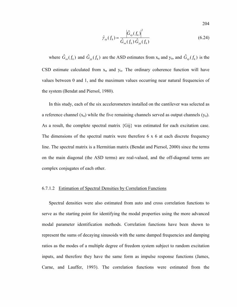
204

)(ˆ)(ˆ)(ˆ

)(ˆ

2

kyykxx

kxykxy fGfG

fGf =γ (6.24)

where )(ˆkxx fG and )(ˆ

kyy fG are the ASD estimates from xn and yn, and )(ˆkxy fG is the

CSD estimate calculated from xn and yn. The ordinary coherence function will have

values between 0 and 1, and the maximum values occurring near natural frequencies of

the system (Bendat and Piersol, 1980).

In this study, each of the six accelerometers installed on the cantilever was selected as

a reference channel (xn) while the five remaining channels served as output channels (yn).

As a result, the complete spectral matrix {Gij} was estimated for each excitation case.

The dimensions of the spectral matrix were therefore 6 x 6 at each discrete frequency

line. The spectral matrix is a Hermitian matrix (Bendat and Piersol, 2000) since the terms

on the main diagonal (the ASD terms) are real-valued, and the off-diagonal terms are

complex conjugates of each other.

6.7.1.2 Estimation of Spectral Densities by Correlation Functions

Spectral densities were also estimated from auto and cross correlation functions to

serve as the starting point for identifying the modal properties using the more advanced

modal parameter identification methods. Correlation functions have been shown to

represent the sums of decaying sinusoids with the same damped frequencies and damping

ratios as the modes of a multiple degree of freedom system subject to random excitation

inputs, and therefore they have the same form as impulse response functions (James,

Carne, and Lauffer, 1993). The correlation functions were estimated from the

205 accelerometers on the cantilever beam using the direct approach outlined by Bendat and

Piersol (2000). An estimate of the autocorrelation function of x(t), where x(t) = x(nΔt) for

n = 1, 2, …, N, for the sample values at the time delay rΔt is given by:

mrxxrN

trR rn

rN

n

nxx ,,2,1,01)(ˆ1

K=−

=Δ +

−

=∑ (6.25)

where r is defined as the lag number and m is the maximum lag number (m < N). This

equation produces an unbiased estimate of the autocorrelation function. The cross-

correlation function between two stationary and zero mean random signals xn and yn may

be estimated from the following expression (for m < N):

mryxrN

trR rn

rN

n

nxy ,,2,1,01)(ˆ1

K=−

=Δ +

−

=∑ (6.26)

After the auto and cross-correlation functions have been estimated, the spectral

densities may be computed by taking the FFT of these functions. The autocorrelation and

cross-correlation functions were computed in Matlab for each excitation case using each

of the six accelerometers as a reference channel (xn). The maximum number of lags (m)

was 8192. The estimated auto and cross-correlation functions were multiplied by an

exponential window prior to the FFT operation to minimize any leakage effects. The

resulting spectral densities computed using this approach served as the starting point for

the identification of the modal properties with the CMIF and PTD methods using the X-

Modal software program. The correlation functions and spectral densities were computed

in a similar fashion from the raw time data records directly in the LMS Test.Lab software

for subsequent modal property identification by the SSI method (Time MDOF algorithm

206 in LMS Test.Lab). The exponential window applied to the time data records of duration T

(the auto and cross-correlation functions), has the form:

τt

ew−

= (6.27)

where t is the time in seconds and τ is the decay time constant (time required for the

signal to decay to a certain percentage of its initial amplitude. In order to compute the

time decay constant required to reduce the signal amplitude at T, A(T) to some

percentage, p, of the initial amplitude A(0), the following expression may be solved:

τ∗= )ln( pT (6.28)

Therefore, to obtain 0.001% of A(0) at T, which was used for the data in this study,

the required time decay constant is computed to be τ = T/11.513.

It must be mentioned that the Hanning and exponential windowing operations

described in the estimation of the frequency spectra will, in effect, add artificial damping

to these spectra. This artificial damping must be accounted for if the spectral estimates

are to be used to identify the damping for the structure being tested. There are standard

approaches for correcting the estimates for these effects; however, since identification of

the damping ratios was not considered in this study, these corrections were not applied to

the spectral estimates.

207 6.7.2 Identification of Modal Parameters

6.7.2.1 Peak-Picking Method

The Peak-Picking (PP) method was implemented using code written in Matlab to

automate the process. The steps utilized for the PP identification are summarized by the

flow chart shown in Figure 6.11. The auto and cross-spectral densities estimated in the

data pre-processing stage serve as the starting point for the PP identification procedure.

The specific procedure that was implemented to identify the natural frequencies and

mode shapes in each excitation case may be described as follows.

First, a parameter matrix that included columns of different mode indicator functions

(MIFs), normalized mode shapes, and coherence functions was created from the

estimated spectral densities. Several different MIFs were computed and used for

comparison purposes, and the details of these are described in following sections. The

mode shapes were computed using each of the output sensors installed on the cantilever

as a separate reference channel. The mode shapes were forced to have normal mode

characteristics by using a whitewashing procedure.

After the parameter matrix was constructed, the next step was to identify the peaks in

the different MIF spectra. This was done in an automated fashion by comparing the MIF

value at every frequency line with the MIF value at a set number of contiguous frequency

lines immediately before and after it. If the MIF value at a given frequency line was

larger than its value at the predetermined number of frequency lines before and after it, it

was identified as a peak location. A total of three different numbers of contiguous

frequency line criteria were utilized for comparison purposes. A minimum threshold level

208 for the MIF values was also specified and used as an additional criterion for selecting the

peaks.

Data Pre-Processing

Spectral Density Matrix

Mode Shape at each

Frequency Line

Coherence Functions

Compute Mode Indicator Functions

(MIFs)

Whitewash Mode Shapes & Unit

Normalize

Identify Peaks in MIFs (3P, 4P, or

5P criteria)

Parameter Matrix

Apply MIF Amplitude Threshold (Optional)

Candidate Natural Frequencies & Mode Shapes

Verif

y N

orm

al M

odes

Coherence ParametersMode ShapesMAC

Parameters

Final Natural Frequencies & Mode Shapes

Dam

ping

Rat

io

Iden

tific

atio

n

Data Pre-ProcessingData Pre-

Processing



Mode Shape at each

Frequency Line

Coherence FunctionsCoherence Functions


(MIFs)


(MIFs)

Whitewash Mode Shapes & Unit

Normalize


5P criteria)


5P criteria)

Parameter Matrix

Parameter Matrix

Apply MIF Amplitude Threshold (Optional)Apply MIF Amplitude Threshold (Optional)



Verif

y N

orm

al M

odes

Coherence ParametersCoherence ParametersMode ShapesMode ShapesMAC

ParametersMAC

Parameters

Final Natural Frequencies & Mode Shapes

Dam

ping

Rat

io

Iden

tific

atio

n

Figure 6.11. Flowchart for PP implementation

209 Once the locations of the peaks in the MIF spectra were identified, several parameters

are computed using ordinary coherence functions and Modal Assurance Criterion (MAC)

values. These parameters are utilized in conjunction the visual examination of the mode

shapes computed using different reference sensors to identify the final natural

frequencies. The raw value of the phase factor (non-whitewashed) computed between

each sensor and a selected reference sensor is checked at each identified peak to verify

that they are indeed normal modes.

Damping ratios were not estimated in this study, although they could be using the

half-power bandwidth method or the random decrement method for the final set of

identified natural frequencies. Additional details for each step in the PP identification

method as implemented for this study are provided in following sections.

Mode Indicator Functions

A numerical function that provides an indication of the locations of natural

frequencies from the estimated spectra may be termed a mode indicator function (MIF).

In this study, a number of different MIFs were evaluated in conjunction with the PP

approach for identifying the natural frequencies of the cantilever beam. A

One MIF that has been used for identifying natural frequencies in ambient vibration

tests of in-service structures is the Averaged Normalized Power Spectral Density

(ANPSD) function developed by Felber (1993). This ANPSD combines the autospectral

density estimates, also referred to as Power Spectral Densities or PSD, from multiple

output channels into a single function suitable for automated identification of spectral

210 peaks. The ANSPD is computed in two steps. First, the estimated PSD from each output

channel (i) is normalized according to the following expression:

)2/(,,2,1,0

)(

)()( 2/

0

Nk

fPSD

fPSDfNPSD Nk

k

ki

kiki K==

∑=

=

(6.29)

In this expression, the PSD value for at each frequency line is normalized by dividing

it by the sum of the PSD values for every frequency line. The ANPSD is then computed

for a group of l output channels by the following expression:

∑=

==l

i

kik NkfNPSDl

fANPSD1

)2/(,,2,1,0)(1)( K (6.30)

The ANPSD function utilizes the diagonal terms of the estimated spectral matrix and

effectively combines the autospectral densities from any sensors used in an ambient

vibration test, whether or not they are deployed in a stationary or roving instrumentation

scheme.

It should be noted that the summation in Eq. (6.30) is by itself adequate for

identifying the locations of the spectral peaks. Dividing the result of summation term in

Eq. (6.30) by the number of channels l (a constant value) has the same effect at every

frequency line; therefore, the averaging operation in the computation of the ANPSD is

unnecessary and redundant. The sum of the NPSD terms will yield exactly the same

number of spectral peaks as the ANPSD.

211 A second MIF that was developed and used for the PP identification was termed the

SPSD function. This MIF represents the simplest combination of the estimated PSD

results for each channel, without any normalization or averaging. This function was

computed to evaluate the effects of normalization and averaging on the effectiveness of

identifying peaks by the ANPSD function. In other words, the SPSD function was

computed to see if it would be any more or less effective than the ANPSD which utilizes

the same basic spectral information with normalization and averaging. The SPSD may be

computed for a group of l output channels at discrete frequency lines k by the following

expression:

∑=

==l

i

kik NkfPSDfSPSD1

)2/(,,2,1,0)()( K (6.31)

A final MIF that was developed and used in this study for the PP identification was

termed the SSCSD function. This MIF was developed to incorporate the multiple

references available when a stationary instrumentation scheme is utilized for ambient

vibration testing. When a stationary instrumentation scheme is utilized, all of the sensors

are measured simultaneously. This permits each sensor channel to be utilized as a

reference for the identification of the modal properties. The objective for utilizing this

function was to evaluate whether or not a multiple reference extension of the basic PP

method would offer any additional advantages in the identification of the natural

frequencies of the beam.

The SSCSD function may be considered as a multiple reference extension of the basic

single reference PP method utilized for ambient vibration tests using a roving

instrumentation scheme. The SSCSD is based on the same fundamental characteristic that

212 enables the PSD and MIFs utilizing the PSD to be used to identify the natural frequencies

of a structure. The CSD, like the PSD, will become a maximum at the spectral lines

corresponding to the locations of natural frequencies for a structure. The SSCSD is

computed in two steps, and utilizes a single row or column of the full spectral matrix for

each reference channel r selected. Because the CSD is a complex number, the magnitude

of the CSD function at each spectral line is utilized in the computation of the SSCSD.

The first step in computing the SSCSD is to compute the sum of the CSD magnitudes

(SCSD) at discrete frequencies for a group of l output sensors with one output sensor r

selected to serve as a reference channel. The SCSD is computed using the following

equation:

∑=

==l

q

kqrkr NkfCSDfSCSD1

)2/(,,2,1,0)()( K (6.32)

If p sensors from the group of l output sensors are selected to serve as references r,

the SSCSD function is computed from the following expression:

∑=

==p

r

krk NkfSCSDfSSCSD1

)2/(,,2,1,0)()( K (6.33)

In this study, all sensors from the group of l output sensors were selected as

references (p = l) for each excitation case, therefore the SSCSD function incorporates the

full spectral matrix estimated from the sensor channels on the cantilever beam.

213 Automatic Identification of Spectral Peaks in MIFs

The locations of spectral peaks in each MIF evaluated for this study were identified

using an automated procedure that compared the value of a MIF at each spectral line with

the value of the same MIF at a number of spectral lines immediately preceding and

following the frequency line being considered. In this study, three criteria were evaluated

for the automatic identification of the spectral peaks in each MIF. Each criterion was

defined by the number of contiguous spectral lines before and after each spectral line that

were compared to automatically identify the peak locations in the MIF. As illustrated in

Figure 6.12, the number of points (MIF value at contiguous spectral lines) before and

after the MIF value at each spectral line that were considered for the automatic

identification of the peaks included cases with 3 points (3P criterion), 4 points (4P

criterion), and 5 points (5P criterion). If the MIF amplitude at a discrete spectral line was

larger than at the specified number of contiguous spectral lines located before and after it,

it was automatically identified as a peak. The values in the parameter matrix shown in

Figure 6.11 corresponding to the locations of spectral peaks were retained for the

subsequent steps in the PP procedure.

A minimum threshold value for the MIF amplitude can also be specified as shown in

Figure 6.13 to reduce the number of identified peaks to only those which meet the 3P, 4P

or 5P criterion and which exceed the minimum threshold value for the MIF amplitude.

The selection of the minimum threshold is a somewhat arbitrary operation, and is not

required for the subsequent stages of the PP method, but it can reduce the number of

spectral peaks that must be considered to only those which exhibit a selected minimum

level of response. In most cases, the number of peaks that must be considered can be

214 substantially reduced by specifying a minimum threshold value. Furthermore, the peaks

that exceed the minimum threshold level will have a larger signal-to-noise ratio and

corresponding level of reliability than the peaks that do not exceed the threshold level.

1

2

3

4

P

ΔfFreq. (Hz)

MIF

Am

plitu

de

1

2

34

4 Point Criterion (4P)

1

2

3

P

ΔfFreq. (Hz)

MIF

Am

plitu

de

1

2

3


Freq. (Hz)

1

2

3

4

P

Δf

MIF

Am

plitu

de

1

2

34


5

5

Mor

e R

estri

ctiv

e Id

entif

icat

ion

1

2

3

4

P

ΔfFreq. (Hz)

MIF

Am

plitu

de

1

2

34


1

2

3

P

ΔfFreq. (Hz)

MIF

Am

plitu

de

1

2

3


Freq. (Hz)

1

2

3

4

P

Δf

MIF

Am

plitu

de

1

2

34


5

5

Mor

e R

estri

ctiv

e Id

entif

icat

ion

Figure 6.12. Criteria for automatic identification of spectral peaks in a MIF

215

1

2

34

P

Δf

Freq. (Hz)

MIF

Am

plitu

de1

2

34

4 Point Criteria (4P)

P

12

3

1

23

4

Threshold Level

Yes

No

1

2

34

P

Δf

Freq. (Hz)

MIF

Am

plitu

de1

2

34

4 Point Criteria (4P)

P

12

3

1

23

4

Threshold Level

Yes

No

Figure 6.13. Application of minimum threshold for automated identification of peaks

Computation and Normalization of Mode Shapes

In this application, mode shapes were computed at every frequency line and placed in

the parameter matrix along with the MIF values for automated identification described in

the previous section. The mode shapes themselves were not utilized as a criterion in the

identification of the natural frequencies, the values were simply computed at every

possible spectral line and the subset corresponding to the identified spectral peaks were

evaluated in subsequent steps of the PP procedure. The mode shapes are in reality

operating deflection shapes (ODS) since more than one natural mode may be contributing

to the measured response. The ODS may be considered as reasonable approximations of

the actual mode shapes for cases where the modes are well-separated.

The mode shapes can be estimated from the magnitude and phase information

contained in a single row or column of the full spectral density matrix. The magnitude of

each term in a row or column will give the relative amplitude of the corresponding

216 measurement degree of freedom relative to the selected reference location. The phase

factor associated with each term indicates the phase characteristics of the associated

measurement degree of freedom relative to the selected reference location. The reference

location in each row or column of the spectral density matrix will be the diagonal term

(the real-valued ASD term) of the full spectral matrix. In this study, the mode shapes

were computed at every frequency line by considering each sensor in the output sensor

group as a reference sensor. Therefore, each row (or column) of the full spectral matrix

was used to create a mode shape of the structure at every frequency line. The mode

shapes computed for each reference at a given frequency line where evaluated for

identifying the natural modes of the structure.

If the phase factor between a given measurement degree of freedom with respect to

the reference location is zero (or very close to zero), the measurement degree of freedom

will be in-phase with the reference degree of freedom. If the phase factor between a given

measurement degree of freedom with respect to the reference location is 180 degrees (or

very close to 180 degrees), the measurement degree of freedom will be out-of-phase with

respect to the reference degree of freedom. In practice, the phase factor will rarely be

exactly equal to zero or 180 degrees which is associated with normal modes, but will

frequently be close to these values. According to Bendat and Piersol (1980), the phase

factor may be used to help distinguish between output spectral peaks that are due to

structural vibration modes and those which are due to spectral peaks in the excitation.

The phase factor between two output sensors will usually be something other than zero or

180 degrees at a spectral peak due to excitation.

217 In the PP procedure implemented for this study, the mode shapes were all forced to

behave as normal modes using a procedure referred to as “whitewashing” (Ewins, 2000).

Whitewashing forces the modes shapes to behave as normal modes by imposing a phase

factor of zero degrees to estimated phase factor values between zero and 90 degrees (or

270 degrees and 360 degrees, and imposing a phase factor of 180 degrees to estimated

phase factor values between 90 degrees and 180 degrees. Forcing the identified modes to

behave as normal modes (as opposed to complex modes where the measurement degrees

of freedom may pass through the zero point at different times) provides a convenient and

consistent means of comparing the experimental results with analytical results. The non-

whitewashed mode shapes associated spectral peaks identified as candidate natural

frequencies should be evaluated to verify that they are indeed due to structural vibration

modes and not due to excitation effects or complex mode behavior. In other words, the

character of the modes associated with candidate natural frequencies should be verified

before they are characterized as being associated with natural frequencies of the structure.

Coherence and MAC Parameters

A number of additional parameters were also computed at the locations of identified

spectral peaks for subsequent use in the identification of the natural frequencies and

mode shapes of the cantilever beam. Bendat and Piersol (1980) note that the value of the

ordinary coherence function given in Eq. (6.24) will tend to peak at the locations of

normal mode frequencies since the signal-to-noise ratio is maximized at these

frequencies. Since the ordinary coherence function may only be computed between one

output sensor and a selected reference sensor, a parameter was developed for use in this

218 study that combined the coherence values computed between each output sensor and

multiple output sensors selected as a references. This parameter, termed the SSCOH

parameter, was computed in two steps. In the first step, the SCOH parameter is computed

at discrete frequencies by taking the sum of the ordinary coherence values for each

channel in the group of l output sensors relative to the selected reference sensor r

according the following equation:

∑=

==l

q

kqrkr NkfCOHfSCOH1

)2/(,,2,1,0)()( K (6.34)

The SSCOH parameter may then be computed for the p number of channels selected

from a group of l output sensors according to the following equation:

∑=

==p

r

krk NkfSCOHfSSCOH1

)2/(,,2,1,0)()( K (6.35)

To simplify the interpretation of the SSCOH parameter for a group of channels with

multiple references, it may be expressed as the percentage of its maximum possible value

(%SSCOH). For example, if all 6 sensors on the cantilever beam are used as references,

there would be a total of 36 coherence values computed, and the maximum possible value

for Eq. (6.35) would be equal to 36 at each discrete frequency line. If the result from Eq.

(6.35) at a particular frequency line was equal to 35, the corresponding %SSCOH value

would be 97.2% (35/36).

The Modal Assurance Criterion (MAC) is another parameter that was used in this

study to assist with the identification of the natural frequencies from the identified

spectral peaks. The MAC is commonly used in experimental modal analysis to evaluate

219 the correlation between experimental and analytical mode shapes. The MAC is a scalar

quantity that provides a measure of the scatter of the points from a straight line

correlation of two mode shape vectors and is given by the following expression (Ewins,

2000):

{ } { }{ } { }( ){ } { }( )A

TAX

TX

AT

XXAMACψψψψ

ψψ2

),( = (6.36)

The MAC will have a value of one if the two vectors are perfectly correlated and a

value of zero if the two vectors are orthogonal. In this study, the MAC is used to evaluate

the correlation of the mode shape vectors computed using a given reference channel with

those computed using other reference channels. There were a total of six output sensor

channels on the cantilever; therefore, there are a total of 36 (the square of the number of

reference channels r selected) MAC values that may be computed at a given frequency

line. These 36 MAC values were summed together at each frequency line, and expressed

as a percentage of the maximum possible value of their sum. Since each MAC value has

a maximum possible value of one, the maximum possible value of the sum of the MAC

values, termed the SMAC, will be equal to the square of the number of reference

channels used. When expressed as the percentage of the maximum possible value of their

sum, the result is designated as the %SMAC.

As mentioned previously, the MAC is most frequently used to evaluate the

correlation between experimental and analytical mode shapes. In this study, the analytical

mode shapes for the cantilever beam were determined by the theoretical solution. A

similar parameter to the SMAC was developed for comparing the mode shapes computed

from the multiple references with the analytical mode shape. There will be r number of

220 experimental mode shapes at each frequency line where r is the number of reference

sensors utilized. If there are m analytical mode shapes to be compared with each

experimental mode shape, a total of r x m MAC values will be computed. The sum of the

MAC value for each analytical mode shape and the r experimental mode shapes at a

discrete frequency may be computed and expressed as a percentage of the maximum

possible sum in a similar fashion as with the SMAC parameter. For example, if mode

shapes are developed using each of the six sensors on the cantilever as a separate

reference sensor, a total of six experimental mode shapes are computed at each frequency

line. If these six mode shapes are compared with one analytical mode shape, the

maximum possible sum of the MAC values will be equal to six if the analytical mode is

perfectly correlated with each experimental mode at that particular frequency line. Since

the experimental mode shapes are compared with the analytical (or theoretical) mode

shapes, this parameter is termed the TMAC. When expressed as the percentage of the

maximum possible value of their sum, the result is designated as the %TMAC for this

study.

6.7.2.2 Advanced Identification Methods

The frequencies and mode shapes were identified using the SSI method (Time MDOF

algorithm) in the commercially available software package TestLab from LMS

(Belgium). The frequencies and mode shapes for each excitation case were identified

using the PTD and CMIF methods as implemented in the software package XModal from

the Structural Dynamic Research Lab (SDRL) at the University of Cincinnati. All of the

221 sensor channels were used as references in for the identification of the dynamic

properties with each advanced identification method.

6.8 Results

6.8.1 Spectral Densities for Excitation Cases

The autospectral densities (ASD) for the pure random and harmonic superimposed on

random excitation cases are shown in Figure 6.14 and Figure 6.15, respectively. The

ASD for the H1 excitation case is shown in Figure 6.16. The ASD from an accelerometer

installed on the linear shaker can be seen in Figure 6.14 and Figure 6.15. The excitation is

not exactly flat as a slight linear trend is observed for the ASD of the linear shaker in

each case. This represents an operational characteristic of the linear shaker used for this

study. It is not unreasonable to expect that the ambient dynamic excitation for an in-

service bridge structure might have a similar characteristic. The frequency band of the

shaker excitation is more precisely defined in each case. The excitation frequency of the

eccentric mass shaker could not be measured directly, although it could be detected by a

peak at approximately 6.25 Hz in the ASD spectra shown in Figure 6.15. The lateral

vibration response of the cantilever tip is shown in Figure 6.15 and Figure 6.16 for

illustration purposes only; this measurement was not used in conjunction with the

identification of the dynamic properties of beam.

222

BB400

NB200

NB50

NB10

Linear Shaker

Linear Shaker

Linear Shaker

Linear Shaker

BB400

NB200

NB50

NB10

Linear Shaker

Linear Shaker

Linear Shaker

Linear Shaker

Figure 6.14. Autospectral density plots for random excitation cases

BB400+H1

NB200+H1

NB50+H1

NB10+H1

Linear Shaker

Linear Shaker

Linear Shaker

Linear Shaker

Lateral

LateralLateral

Lateral

BB400+H1

NB200+H1

NB50+H1

NB10+H1

Linear Shaker

Linear Shaker

Linear Shaker

Linear Shaker

Lateral

LateralLateral

Lateral

Figure 6.15. Autospectral density plots for random excitation cases with superimposed harmonic excitation

223

Lateral Response at Tip

Eccentric Mass Shaker Input Not Measured

(H1)Lateral Response at Tip


(H1)Lateral Response at Tip


(H1)

Figure 6.16. Autospectral density plot for H1 excitation case

6.8.2 Peak Selection Criteria and Mode Indicator Functions

The number of spectral peaks identified using the automated PP criteria with different

MIFs for each excitation case is summarized in Table 6.3. The quantities given in the

table were not subject to a minimum MIF amplitude threshold criterion. They are simply

the number of peaks that were identified by comparing the amplitudes of the MIFs for

different quantities of contiguous spectral lines. Although the number of identified peaks

decreases when a more stringent selection criteria is applied (5P versus 3P), the

frequencies corresponding to the first five analytical modes of the beam are included in

each set of results.

It is clear from the Table 6.3 that the number of spectral peaks identified using the

different MIFs are very comparable to each other. Since the population of spectral peaks

identified by each MIF contained the five natural frequencies of the cantilever beam, the

224 remaining peaks represent spurious results or peaks in the excitation. Thus, the number of

peaks identified using a given MIF beyond the five natural frequencies provides a

measure of the efficiency of the MIF. The MIF that leads to the identification of the

largest number of spurious peaks can be considered to be the least efficient. The ANPSD

function, on average, led to the identification of slightly more peaks than the SPSD and

SSCSD for a given excitation case and selection criterion; however, the difference is too

small (generally less than 10 peaks) to consider any one of the MIFs used to be superior

to the others.

The number of peaks identified from the excitation cases containing the

superimposed harmonic component (H1) was generally less than the number identified in

the purely random excitation counterparts. This is most likely the result of more

excitation energy being transmitted into the cantilever when the eccentric mass shaker

was combined with the linear shaker.

A minimum threshold criterion was applied to the amplitudes of the MIFs that

resulted in the initial peak identification. Since the amplitude scale associated with each

MIF was slightly different, the minimum amplitude threshold level for each MIF was

iteratively adjusted to a different unit power of 10 (i.e. 1x10-6, 1x10-5, 1x10-4, etc.) that

until the remaining peaks identified for each MIF contained the known natural

frequencies for the cantilever. The number of peaks identified for each MIF using the 4P

selection criterion and a minimum threshold level for each excitation case is summarized

in Table 6.4.

It is clear from the results shown in the table that the number of spectral peaks can be

reduced significantly by utilizing a minimum threshold for the peak picking process. The

225 reduction in the number of peaks after the application of the amplitude threshold is

similar for each MIF within a given excitation case. There is some justification for

applying a minimum amplitude threshold since it will filter any peaks associated with

low level responses (less reliable information).

The threshold criterion does not reduce the number of spectral peaks for the random

excitation case with superimposed harmonic as dramatically as it does for the purely

random excitation cases. The former excitation cases may simply have more noise related

peaks with higher amplitudes than the latter excitation cases, and the level threshold

would therefore not be as effective in such cases. This would also be consistent with the

earlier observation that the eccentric mass shaker transmits more excitation energy into

the cantilever. More transmitted energy will lead to spurious peaks with larger amplitudes

in addition to the larger structural responses.

A final observation that may be made relative to the application of a minimum

amplitude threshold criterion relates to the efficiency of each MIF. It is clear that the

ANPSD is generally less efficient (more spurious peaks) than the other two MIFs for the

pure random excitation cases, and is significantly less efficient than the other two for the

random excitation with superimposed harmonic excitation cases. This is most likely due

to the normalization of the ASDs that is done when computing the ANPSD function.

Normalization effectively brings each ASD and any noise in the spectra to a common

level making the application of a minimum amplitude threshold less effective than with

the other MIFs.

226

Table 6.3. Number of spectral peaks identified by selection criterion and MIF

Mode Indicator Function (MIF) Excitation case

Selection criterion ANPSD SPSD SSCSD

3P 462 451 450 BB400 4P 349 347 348 5P 285 281 283 3P 517 505 508 NB200 4P 411 386 384 5P 348 323 333 3P 512 507 510 NB50 4P 395 388 404 5P 324 318 328 3P 504 507 496 NB10 4P 397 395 385 5P 335 324 309 BB400+H1 4P 337 331 328 NB200+H1 4P 330 310 312 NB50+H1 4P 316 305 302 NB10+H1 4P 315 315 320 H1 4P 344 337 337

Table 6.4. Number of spectral peaks identified for each MIF with minimum threshold criterion

Mode Indicator Function (MIF) Excitation case

Selection criterion ANPSD SPSD SSCSD

BB400 4P 14 19 25 NB400+H1 4P 140 86 114 NB200 4P 46 35 47 NB200+H1 4P 69 19 22 BB50 4P 40 32 39 NB50+H1 4P 67 60 20 NB10 4P 36 29 35 NB10+H1 4P 78 19 22 H1 4P 143 91 119

227 6.8.3 Natural Frequencies and Mode Shapes

6.8.3.1 Random Dynamic Excitation Cases

BB400 Excitation Case

The spectral peaks identified by the automated PP procedure for the BB400 excitation

case according to each MIF are summarized in Table 6.5. The spectral peaks were

identified using the 4P selection criterion with a minimum MIF amplitude level threshold

specified. The spectral peaks identified by each MIF include the five theoretical natural

frequencies of the cantilever beam plus different quantities of spurious spectral peaks. If

the locations of the natural frequencies are not known a priori with great confidence, as is

generally the case in an ambient vibration test of an in-service structure, the population of

identified spectral peaks must be further scrutinized to identify the subset that correspond

to the natural frequencies of the structure being testing.

One of the most efficient means for scrutinizing the population of identified spectral

peaks to identify the natural frequencies may be to visually examine the mode shapes that

correspond to each spectral peak. In this study, the mode shapes were constructed using

each output sensor on the cantilever as a reference sensor, so there are effectively five

discrete mode shapes computed for each spectral peak.

228 Table 6.5. Spectral peaks by PP for BB400 excitation case

4P Selection Criterion with Minimum MIF Level Amplitude Threshold Frequency with peak in MIF (Hz)

Peak number ANPSD SPSD SSCSD 1 4.688 4.688 4.688 2 13.379 7.324 7.324 3 18.164 10.547 10.547 4 18.945 13.379 13.379 5 21.875 18.164 18.164 6 26.367 21.875 18.945 7 29.297 23.047 19.922 8 29.785 24.219 21.289 9 82.617 24.902 21.875

10 85.254 26.367 23.047 11 120.020 27.148 24.219 12 160.840 29.297 24.902 13 240.039 29.785 26.367 14 260.938 82.617 27.148 15 85.254 29.297 16 120.020 29.785 17 160.840 82.617 18 240.039 84.668 19 260.938 85.254 20 88.184 21 120.020 22 160.840 23 162.207 24 240.039 25 260.938

The mode shapes associated with the 14 spectral peaks identified by PP using the

ANPSD function (the most efficient MIF for this particular excitation case) are shown in

Figure 6.17. The mode shapes corresponding to the natural frequencies of the cantilever

beam are highlighted in each figure. It is clear from visual inspection that mode shapes

associated with many of the spectral peaks shown in these figures may be ruled out as

possible natural frequencies. In particular, the identified spectral peaks at 18.164 Hz,

18.945 Hz and 21.875 Hz at may be excluded due to a lack of agreement between the 6

different mode shapes computed from each reference sensor at these frequencies. There is

clearly a pattern for the mode shapes shown in Figure 6.17 that indicates that the shapes

associated with natural frequencies of the cantilever are the same irregardless of the

229 reference channel utilized. Moving away from the natural frequencies of the cantilever,

the individual mode shapes generated for different reference channels tend to diverge.

Thus, it may be observed that the mode shapes generated by different reference channels

will tend to snap together and form a single consistent shape at a natural frequency of the

structure provided if the structure has been sufficiently excited. This is because at

resonance, the signal-to-noise ratio of each output sensor will be maximized. The mode

shapes computed for each of the remaining identified spectral peaks in this excitation

case are consistent and cannot be immediately excluded based on this reasoning.

The sensor at the support location will always have the least amount of response at

any frequency and is therefore particularly sensitive to the signal-to-noise ratio of the

response. Furthermore, since this sensor is at the support location, there should be zero or

near zero amplitude at this location in the mode shapes associated with the natural

frequencies. This characteristic may be used to rule out the spectral peaks at 120.020 Hz

and 240.039 Hz as being associated with a natural frequency of the cantilever due to the

physical implausibility of the modal amplitude at the support degree of freedom. The

mode shapes at some of the other spectral peaks (13.379 Hz, 26.367 Hz, 85.254 Hz, and

260.938 Hz) show some nonzero modal amplitude at the support location; however, the

amplitude is small and is consistent with the noise level that is locked into each sensor.

A total of 5 spectral peaks may be ruled out as possible natural frequencies due to

internal inconsistency (agreement of the modes shapes due to each reference sensor) and

physical implausibility of the amplitude at the support degree of freedom. The next

logical step for visually evaluating the mode shapes at the remaining 9 spectral peaks is

to group the spectral peaks according to fundamental shapes. For example, the mode

230 shapes associated with the spectral peak at 4.688 Hz are unique relative to the remaining

spectral peaks. Furthermore, these mode shapes are consistent with the first fundamental

mode shape of the cantilever (zero inflection points away from the support). The mode

shapes at 13.379 Hz, 26.367 Hz, 29.297 Hz and 29. 785 Hz have the same basic shape

that is consistent with the 2nd fundamental mode of the cantilever (one inflection point).

Therefore, these frequencies may be grouped together to form candidate frequencies for

the 2nd natural frequency of the beam. The remaining spectral peaks and mode shapes

may be grouped in a similar fashion as follows: 82.617 Hz and 85.254 Hz (3rd

fundamental mode), 160.840 (4th fundamental mode), and 260.938 (5th fundamental

mode).

It should be obvious that the spectral peaks at 4.688 Hz, 160.840 Hz, and 260.938 Hz

may be considered to be the 1st, 4th and 5th natural frequencies and mode shapes of the

cantilever, since they are the only possible candidates that remain for each of these

modes. There are more than one candidate spectral peaks for the 2nd and 3rd natural

frequencies of the cantilever so further scrutiny is required to identify these natural

frequencies. This requires that additional parameters associated with each spectral peak

be evaluated to identify the most likely natural frequencies.

A summary of the MIF amplitudes, coherence parameters and MAC parameters

associated with the 14 spectral peaks initially identified by the automated PP procedure is

provided in Table 6.6. The spectral peaks that still require scrutiny after the initial visual

analysis of the mode shapes are 13.379 Hz, 26.367 Hz, 29.297 Hz and 29.785 Hz for the

2nd mode, and 82.617 Hz and 85.254 Hz for the 3rd mode. The amplitude of the MIF

should be largest at the true natural frequency of the structure due to resonance. The MIF

231 amplitude at 29.297 Hz is at least an order of magnitude larger than the MIF amplitudes

at the other candidate frequencies for the 2nd mode of the cantilever. The value of the

%SSCOH parameter at 29.297 Hz is relatively high at 94.3% of the maximum possible

sum of the coherence computed for each sensor used as a reference, but the largest value

for the mode shape group occurs at 13.379 Hz. The %SMAC values are essentially the

same at 100% of the maximum possible value for each frequency in this group. The

%TMAC value at 29.297 Hz is 99.7% of the maximum possible value when compared

with the 2nd theoretical mode shape. This value is high, although the %TMAC value for

the 2nd theoretical mode is slightly larger at 29.785 Hz.

In comparing these different parameters for identifying the natural frequency

corresponding to the 2nd mode of the cantilever, the greatest weight should be assigned to

the value of the MIF amplitude, since this is fundamentally related to the signal-to-noise

characteristics of the peak which in turn is related to resonant behavior. Since the peak at

13.379 Hz is not close to the known theoretical 2nd mode of the structure it is a spurious

peak. This indicates that coherence parameter may be high at spurious spectral peaks in

addition to natural frequencies; therefore, this parameter should be given lower weight in

the selection process. The %SMAC values are correlated with the consistency of the

multiple mode shapes generated at each frequency line by using different sensors as

references, and the initial visual evaluation of spectral peaks had already revealed that the

mode shapes were consistent at each of these spectral peaks. This observation is

confirmed by the %SMAC values. The %TMAC parameter provides a good indicator of

which theoretical mode shape each spectral peak will be most likely correlated with, the

fact that an analytical (or theoretical) and experimental mode shapes are being compared

232 does not guarantee that the actual structure behaves the same as its analytical or

theoretical counterpart. As a result, the %TMAC parameter should be given the least

weight of the available parameters for identifying the experimental natural frequencies.

A similar analysis may be done for the two spectral peaks that are candidates for the

3rd mode of the cantilever (82.617 Hz and 85.254 Hz). Considering the parameter values

given in Table 6.6 for these frequencies, it is apparent that the peak at 82.617 Hz is more

likely the 3rd natural frequency for the cantilever beam.

The possible natural frequencies and mode shapes of the cantilever beam identified

for this excitation case using the SSI, CMIF and PTD algorithms are shown in Figure

6.18, Figure 6.19, and Figure 6.20, respectively. A total of 8 possible natural frequencies

and corresponding mode shapes were identified by the SSI method as shown in Figure

6.18. Since there are at most 5 natural frequencies for the cantilever beam in the

frequency range considered, three of the identified frequencies must correspond to

spurious results. The results shown for 120.010 Hz and 240.040 Hz may be excluded by

visual evaluation of the shapes as the support measurement degree of freedom has

physically implausible displacements in each. The mode shapes shown at 13.405 Hz and

29.449 Hz have similar shapes that are consistent with the 2nd mode of the beam. The

only way to select the actual 2nd mode (29.449 Hz) from these two shapes is to utilize the

characteristic that the amplitude of the various degrees of freedom on the cantilever will

be a maximum at resonance. This permits the mode shape at 13.405 Hz to be ruled out as

the 2nd mode since the amplitude of the unit normalized mode shape is smaller between

the fixed support and the tip than for the mode shape at 29.449 Hz. It should be noted that

233 the parameters based on coherence or MAC values are not computed with the SSI

algorithm, and this may limit its effectiveness if repeated mode shapes are identified.

A total of 10 possible natural frequencies were identified by the CMIF method as

shown in Figure 6.19. The mode shapes associated with these frequencies are generally

inconsistent with the theoretical modes for the cantilever. While the frequencies

corresponding to the five modes of the cantilever are identified, the mode shapes

corresponding to only the first two modes are present in the results. In addition, the first

two theoretical mode shapes are repeated at more than one identified peak. The five

natural frequencies of the cantilever can only be reliably identified from these results by

using the theoretical results as a guide, or by considering the results of the PP or SSI

identification. Only two of the mode shapes are consistent with the expected shapes.

Table 6.6. Characteristics of spectral peaks identified for BB400 excitation case

Peak Freq. (Hz)

MIF Amplitude

(g2/Hz) %SSCOH %SMAC

% TMAC

M1

% TMAC

M2

% TMAC

M3

% TMAC

M4

% TMAC

M5 1 4.688 8.6E-02 93.4 100.0 100.0 9.6 11.9 12.5 11.7 2 13.379 3.9E-03 98.9 100.0 58.7 69.2 8.0 22.3 12.9 3 18.164 1.4E-03 83.7 98.3 17.4 81.9 1.8 19.3 6.1 4 18.945 1.3E-03 78.2 95.6 15.6 81.1 1.9 18.5 5.9 5 21.875 1.6E-03 88.9 99.6 13.4 89.5 2.9 17.7 7.0 6 26.367 2.9E-03 98.8 100.0 11.1 97.1 6.1 15.7 9.2 7 29.297 7.3E-02 94.3 100.0 10.4 99.7 9.9 14.0 11.2 8 29.785 7.1E-02 82.8 100.0 10.3 99.8 10.5 13.8 11.5 9 82.617 4.9E-03 99.5 100.0 10.4 13.3 99.5 10.6 15.6

10 85.254 1.2E-03 99.5 100.0 10.8 12.6 99.8 13.1 14.7 11 120.020 1.7E-02 100.0 100.0 9.1 7.6 39.1 52.1 3.4 12 160.840 1.2E-03 99.5 100.0 10.9 11.4 14.7 99.2 8.5 13 240.039 4.0E-02 100.0 100.0 10.3 12.1 10.8 27.7 85.9 14 260.938 1.2E-03 99.9 100.0 9.8 11.1 12.8 15.6 99.3

Natural frequencies and the associated peak amplitude, coherence and MAC parameters are shown in bold

234

4.688 Hz

-1.0

-0.5

0.0

0.5

1.0

0 20 40 60 80 100 120

Ch1 Ch2 Ch3 Ch4 Ch5 Ch6

Uni

t Nor

mal

ized

Am

plitu

de

Distance from Support (in)

13.379 Hz

-1.0

-0.5

0.0

0.5

1.0

0 20 40 60 80 100 120

Ch1 Ch2Ch3 Ch4Ch5 Ch6

18.164 Hz

-1.0

-0.5

0.0

0.5

1.0

0 20 40 60 80 100 120


29.297 Hz

-1.0

-0.5

0.0

0.5

1.0

0 20 40 60 80 100 120


29.785 Hz

-1.0

-0.5

0.0

0.5

1.0

0 20 40 60 80 100 120


82.617 Hz

-1.0

-0.5

0.0

0.5

1.0

0 20 40 60 80 100 120


18.945 Hz

-1.0

-0.5

0.0

0.5

1.0

0 20 40 60 80 100 120


21.875 Hz

-1.0

-0.5

0.0

0.5

1.0

0 20 40 60 80 100 120


26.367 Hz

-1.0

-0.5

0.0

0.5

1.0

0 20 40 60 80 100 120


160.840 Hz

-1.0

-0.5

0.0

0.5

1.0

0 20 40 60 80 100 120


120.020 Hz

-1.0

-0.5

0.0

0.5

1.0

0 20 40 60 80 100 120


85.254 Hz

-1.0

-0.5

0.0

0.5

1.0

0 20 40 60 80 100 120


240.039 Hz

-1.0

-0.5

0.0

0.5

1.0

0 20 40 60 80 100 120


260.938 Hz

-1.0

-0.5

0.0

0.5

1.0

0 20 40 60 80 100 120


4.688 Hz

-1.0

-0.5

0.0

0.5

1.0

0 20 40 60 80 100 120


Uni

t Nor

mal

ized

Am

plitu

de


4.688 Hz

-1.0

-0.5

0.0

0.5

1.0

0 20 40 60 80 100 120


Uni

t Nor

mal

ized

Am

plitu

de


13.379 Hz

-1.0

-0.5

0.0

0.5

1.0

0 20 40 60 80 100 120


18.164 Hz

-1.0

-0.5

0.0

0.5

1.0

0 20 40 60 80 100 120


29.297 Hz

-1.0

-0.5

0.0

0.5

1.0

0 20 40 60 80 100 120


29.297 Hz

-1.0

-0.5

0.0

0.5

1.0

0 20 40 60 80 100 120


29.785 Hz

-1.0

-0.5

0.0

0.5

1.0

0 20 40 60 80 100 120


82.617 Hz

-1.0

-0.5

0.0

0.5

1.0

0 20 40 60 80 100 120


82.617 Hz

-1.0

-0.5

0.0

0.5

1.0

0 20 40 60 80 100 120


18.945 Hz

-1.0

-0.5

0.0

0.5

1.0

0 20 40 60 80 100 120


21.875 Hz

-1.0

-0.5

0.0

0.5

1.0

0 20 40 60 80 100 120


26.367 Hz

-1.0

-0.5

0.0

0.5

1.0

0 20 40 60 80 100 120


160.840 Hz

-1.0

-0.5

0.0

0.5

1.0

0 20 40 60 80 100 120


160.840 Hz

-1.0

-0.5

0.0

0.5

1.0

0 20 40 60 80 100 120


120.020 Hz

-1.0

-0.5

0.0

0.5

1.0

0 20 40 60 80 100 120


85.254 Hz

-1.0

-0.5

0.0

0.5

1.0

0 20 40 60 80 100 120


240.039 Hz

-1.0

-0.5

0.0

0.5

1.0

0 20 40 60 80 100 120


260.938 Hz

-1.0

-0.5

0.0

0.5

1.0

0 20 40 60 80 100 120


260.938 Hz

-1.0

-0.5

0.0

0.5

1.0

0 20 40 60 80 100 120


Figure 6.17. Possible natural frequencies and mode shapes by PP (BB400 excitation case)

235

4.735 Hz

-1.0

-0.5

0.0

0.5

1.0

0 20 40 60 80 100 120

Uni

t Nor

mal

ized

Am

plitu

de


13.405 Hz

-1.0

-0.5

0.0

0.5

1.0

0 20 40 60 80 100 120

29.449 Hz

-1.0

-0.5

0.0

0.5

1.0

0 20 40 60 80 100 120

82.742 Hz

-1.0

-0.5

0.0

0.5

1.0

0 20 40 60 80 100 120

120.010 Hz

-1.0

-0.5

0.0

0.5

1.0

0 20 40 60 80 100 120

160.880 Hz

-1.0

-0.5

0.0

0.5

1.0

0 20 40 60 80 100 120

240.040 Hz

-1.0

-0.5

0.0

0.5

1.0

0 20 40 60 80 100 120

260.860 Hz

-1.0

-0.5

0.0

0.5

1.0

0 20 40 60 80 100 120

Figure 6.18. Possible natural frequencies and mode shapes by SSI (BB400 excitation case)

236

4.659 Hz

-1.0

-0.5

0.0

0.5

1.0

0 20 40 60 80 100 120

14.206 Hz

-1.0

-0.5

0.0

0.5

1.0

0 20 40 60 80 100 120

26.553 Hz

-1.0

-0.5

0.0

0.5

1.0

0 20 40 60 80 100 120

Uni

t Nor

mal

ized

Am

plitu

de


29.321 Hz

-1.0

-0.5

0.0

0.5

1.0

0 20 40 60 80 100 120

29.5 Hz

-1.0

-0.5

0.0

0.5

1.0

0 20 40 60 80 100 120

83.707 Hz

-1.0

-0.5

0.0

0.5

1.0

0 20 40 60 80 100 120

121.775 Hz

-1.0

-0.5

0.0

0.5

1.0

0 20 40 60 80 100 120

163.786 Hz

-1.0

-0.5

0.0

0.5

1.0

0 20 40 60 80 100 120

239.976 Hz

-1.0

-0.5

0.0

0.5

1.0

0 20 40 60 80 100 120

261.221 Hz

-1.0

-0.5

0.0

0.5

1.0

0 20 40 60 80 100 120

4.659 Hz

-1.0

-0.5

0.0

0.5

1.0

0 20 40 60 80 100 120

14.206 Hz

-1.0

-0.5

0.0

0.5

1.0

0 20 40 60 80 100 120

26.553 Hz

-1.0

-0.5

0.0

0.5

1.0

0 20 40 60 80 100 120

Uni

t Nor

mal

ized

Am

plitu

de


29.321 Hz

-1.0

-0.5

0.0

0.5

1.0

0 20 40 60 80 100 120

29.5 Hz

-1.0

-0.5

0.0

0.5

1.0

0 20 40 60 80 100 120

83.707 Hz

-1.0

-0.5

0.0

0.5

1.0

0 20 40 60 80 100 120

121.775 Hz

-1.0

-0.5

0.0

0.5

1.0

0 20 40 60 80 100 120

163.786 Hz

-1.0

-0.5

0.0

0.5

1.0

0 20 40 60 80 100 120

239.976 Hz

-1.0

-0.5

0.0

0.5

1.0

0 20 40 60 80 100 120

261.221 Hz

-1.0

-0.5

0.0

0.5

1.0

0 20 40 60 80 100 120

Figure 6.19. Possible natural frequencies and mode shapes by CMIF (BB400 excitation case)

237 4.737 Hz

-1.0

-0.5

0.0

0.5

1.0

0 20 40 60 80 100 120

13.539 Hz

-1.1

-0.6

-0.1

0.5

1.0

0 20 40 60 80 100 120

29.633 Hz

-1.0

-0.5

0.0

0.5

1.0

0 20 40 60 80 100 120

Uni

t Nor

mal

ized

Am

plitu

de


82.748 Hz

-1.0

-0.5

0.0

0.5

1.0

0 20 40 60 80 100 120

120.008 Hz

-1.0

-0.5

0.0

0.5

1.0

0 20 40 60 80 100 120

160.881 Hz

-1.0

-0.5

0.0

0.5

1.0

0 20 40 60 80 100 120

240.046 Hz

-1.0

-0.5

0.0

0.5

1.0

0 20 40 60 80 100 120

180.031 Hz

-1.0

-0.5

0.0

0.5

1.0

0 20 40 60 80 100 120

260.819 Hz

-1.0

-0.5

0.0

0.5

1.0

0 20 40 60 80 100 120

4.737 Hz

-1.0

-0.5

0.0

0.5

1.0

0 20 40 60 80 100 120

13.539 Hz

-1.1

-0.6

-0.1

0.5

1.0

0 20 40 60 80 100 120

29.633 Hz

-1.0

-0.5

0.0

0.5

1.0

0 20 40 60 80 100 120

Uni

t Nor

mal

ized

Am

plitu

de


82.748 Hz

-1.0

-0.5

0.0

0.5

1.0

0 20 40 60 80 100 120

120.008 Hz

-1.0

-0.5

0.0

0.5

1.0

0 20 40 60 80 100 120

160.881 Hz

-1.0

-0.5

0.0

0.5

1.0

0 20 40 60 80 100 120

240.046 Hz

-1.0

-0.5

0.0

0.5

1.0

0 20 40 60 80 100 120

180.031 Hz

-1.0

-0.5

0.0

0.5

1.0

0 20 40 60 80 100 120

260.819 Hz

-1.0

-0.5

0.0

0.5

1.0

0 20 40 60 80 100 120

Figure 6.20. Possible natural frequencies and mode shapes by PTD (BB400 excitation case)

The PTD method led to the identification of 9 possible natural frequencies as shown

in Figure 6.20. As was the case with the CMIF method, the frequencies corresponding to

the first five modes are contained in the results. Furthermore, the mode shapes

corresponding to only the first two modes of the cantilever beam are contained in the

results. The results from the PTD method can only be interpreted reliably using the

theoretical results or the results from the PP and SSI methods as a guide.

238 NB200 Excitation Case

The final natural frequencies and mode shapes identified by the automated PP

procedure for the NB200 excitation case are shown in Figure 6.21. These modes

represent a subset of a much larger initial pool of candidate spectral peaks that were

identified by the PP procedure. It should be noted that only the first four modes of the

cantilever beam are identified by PP for this excitation case. The 5th mode of the structure

is located at a frequency that was outside of the frequency band of the supplied dynamic

excitation. The frequency corresponding to the 5th mode was identified by PP based on

the 4P selection criteria (there is a peak in the MIF functions at this frequency), but was

subsequently filtered out by the application of a minimum MIF amplitude level threshold

criterion. This result lends credence to the observation that the PP approach as

implemented for this study is theoretically sound. Only the most reliable natural

frequencies (those with the most energy or signal-to-noise ratio) are identified by PP for

this excitation case.

The frequencies and corresponding mode shapes identified by the SSI method are

shown in Figure 6.22. It is possible to exclude the frequency and mode shape identified at

240.000 Hz due by visual examination of the corresponding mode shape. The frequency

at 13.606 Hz may also be ruled out in favor of the frequency at 29.144 Hz using similar

reasoning as was employed for the BB400 excitation case with this method. It is notable

that the 5th mode of the cantilever beam and its mode shape are identified by this

approach; however, it may be argued that this should not be the case due to the excitation

bandwidth, and that the reliability of the mode and any related parameters (such as

damping) may not be adequate. This indicates a possible deficiency with the SSI

239 approach in that although it is able to extract the correct 5th natural frequency and mode

shape for the cantilever, it does not provide any indication to the analyst that this result

may not have the same level of reliability associated with it as the other frequencies and

mode shapes that were identified. Such information would be very meaningful if the

results are used for subsequent calibration of analytical or finite element models of the

structure.

The possible natural frequencies and mode shapes that were identified by the CMIF

method for the NB200 excitation case are shown in Figure 6.23. Only the frequencies

associated with the 1st, 2nd, and 3rd modes are identified in this excitation case.

Furthermore, only mode shapes that are consistent with the 1st and 2nd mode of the

cantilever are identified. It is only possible to interpret the results of this approach in

conjunction with the theoretical results or those obtained from the PP and SSI methods.

Figure 6.24 shows the possible natural frequencies identified by the PTD method for

the NB200 excitation case. The frequencies corresponding to all five modes of the

cantilever are identified by this method, but only the first two mode shapes are contained

in the identification results. As was observed for the CMIF method, the results obtained

from this method can only be interpreted in conjunction with the theoretical results or

with the results of the PP or SSI method. The PTD and CMIF methods also do not

provide any indication of the reliability of the identified results as was the case with the

SSI method. The identification of the modal properties is clearly not as transparent for the

SSI, PTD, and CMIF approaches as it is in the PP method.

240

160.156 Hz

-1.0

-0.5

0.0

0.5

1.0

0 20 40 60 80 100 120


82.813 Hz

-1.0

-0.5

0.0

0.5

1.0

0 20 40 60 80 100 120


4.688 Hz

-1.0

-0.5

0.0

0.5

1.0

0 20 40 60 80 100 120


29.785 Hz

-1.0

-0.5

0.0

0.5

1.0

0 20 40 60 80 100 120


Uni

t Nor

mal

ized

Am

plitu

de


160.156 Hz

-1.0

-0.5

0.0

0.5

1.0

0 20 40 60 80 100 120


82.813 Hz

-1.0

-0.5

0.0

0.5

1.0

0 20 40 60 80 100 120


4.688 Hz

-1.0

-0.5

0.0

0.5

1.0

0 20 40 60 80 100 120


29.785 Hz

-1.0

-0.5

0.0

0.5

1.0

0 20 40 60 80 100 120


Uni

t Nor

mal

ized

Am

plitu

de


Figure 6.21. Experimental natural frequencies and mode shapes by PP (NB200 excitation case)

4.726 Hz

-1.0

-0.5

0.0

0.5

1.0

0 20 40 60 80 100 120

13.606 Hz

-1.0

-0.5

0.0

0.5

1.0

0 20 40 60 80 100 120

29.144 Hz

-1.0

-0.5

0.0

0.5

1.0

0 20 40 60 80 100 120

82.973 Hz

-1.0

-0.5

0.0

0.5

1.0

0 20 40 60 80 100 120

160.200 Hz

-1.0

-0.5

0.0

0.5

1.0

0 20 40 60 80 100 120

240.000 Hz

-1.0

-0.5

0.0

0.5

1.0

0 20 40 60 80 100 120

260.580 Hz

-1.0

-0.5

0.0

0.5

1.0

0 20 40 60 80 100 120

Uni

t Nor

mal

ized

Am

plitu

de


4.726 Hz

-1.0

-0.5

0.0

0.5

1.0

0 20 40 60 80 100 120

13.606 Hz

-1.0

-0.5

0.0

0.5

1.0

0 20 40 60 80 100 120

29.144 Hz

-1.0

-0.5

0.0

0.5

1.0

0 20 40 60 80 100 120

82.973 Hz

-1.0

-0.5

0.0

0.5

1.0

0 20 40 60 80 100 120

160.200 Hz

-1.0

-0.5

0.0

0.5

1.0

0 20 40 60 80 100 120

240.000 Hz

-1.0

-0.5

0.0

0.5

1.0

0 20 40 60 80 100 120

260.580 Hz

-1.0

-0.5

0.0

0.5

1.0

0 20 40 60 80 100 120

Uni

t Nor

mal

ized

Am

plitu

de


Figure 6.22. Possible natural frequencies and mode shapes by SSI (NB200 excitation case)

241 4.654 Hz

-1.0

-0.5

0.0

0.5

1.0

0 20 40 60 80 100 120

14.405 Hz

-1.0

-0.5

0.0

0.5

1.0

0 20 40 60 80 100 120

26.034 Hz

-1.0

-0.5

0.0

0.5

1.0

0 20 40 60 80 100 120

29.419 Hz

-1.0

-0.5

0.0

0.5

1.0

0 20 40 60 80 100 120

29.555 Hz

-1.0

-0.5

0.0

0.5

1.0

0 20 40 60 80 100 120

85.312 Hz

-1.0

-0.5

0.1

0.6

1.1

0 20 40 60 80 100 120

84.233 Hz

-1.0

-0.5

0.0

0.5

1.0

0 20 40 60 80 100 120

106.425 Hz

-1.0

-0.5

0.0

0.5

1.0

0 20 40 60 80 100 120

82.983 Hz

-1.0

-0.5

0.0

0.5

1.0

0 20 40 60 80 100 120

Uni

t Nor

mal

ized

Am

plitu

deDistance from Support (in)

146.68 Hz

-1.0

-0.5

0.0

0.5

1.0

0 20 40 60 80 100 120

117.104 Hz

-1.0

-0.5

0.0

0.5

1.0

0 20 40 60 80 100 120

Figure 6.23. Possible natural frequencies and mode shapes by CMIF (NB200 excitation case)

242 4.727 Hz

-1.0

-0.5

0.0

0.5

1.0

0 20 40 60 80 100 120

7.273 Hz

-1.0

-0.5

0.0

0.5

1.0

0 20 40 60 80 100 120

29.502 Hz

-1.0

-0.5

0.0

0.5

1.0

0 20 40 60 80 100 120

83.042 Hz

-1.0

-0.5

0.0

0.5

1.0

0 20 40 60 80 100 120

120.000 Hz

-1.0

-0.5

0.0

0.5

1.0

0 20 40 60 80 100 120

160.250 Hz

-1.0

-0.5

0.0

0.5

1.0

0 20 40 60 80 100 120

239.998 Hz

-1.0

-0.5

0.0

0.5

1.0

0 20 40 60 80 100 120

260.539 Hz

-1.0

-0.5

0.0

0.5

1.0

0 20 40 60 80 100 120


4.727 Hz

-1.0

-0.5

0.0

0.5

1.0

0 20 40 60 80 100 120

7.273 Hz

-1.0

-0.5

0.0

0.5

1.0

0 20 40 60 80 100 120

29.502 Hz

-1.0

-0.5

0.0

0.5

1.0

0 20 40 60 80 100 120

83.042 Hz

-1.0

-0.5

0.0

0.5

1.0

0 20 40 60 80 100 120

120.000 Hz

-1.0

-0.5

0.0

0.5

1.0

0 20 40 60 80 100 120

160.250 Hz

-1.0

-0.5

0.0

0.5

1.0

0 20 40 60 80 100 120

239.998 Hz

-1.0

-0.5

0.0

0.5

1.0

0 20 40 60 80 100 120

260.539 Hz

-1.0

-0.5

0.0

0.5

1.0

0 20 40 60 80 100 120


Figure 6.24. Possible natural frequencies and mode shapes by PTD (NB200 excitation case)

NB50 Excitation Case

The final set of experimental natural frequencies and mode shapes identified by PP

for the NB50 excitation case are shown in Figure 6.25. The first four modes of the

cantilever beam are identified from this excitation case by PP, although the frequency

band of the excitation should have been adequate to only identify the first two modes. It

is apparent from the mode shapes shown in Figure 25 that enough energy was supplied

into the system to reliably identify the 3rd and 4th modes of the cantilever beam. The

frequency of the 5th mode of the cantilever was identified by the initial PP procedure, but

was subsequently filtered from the final results by the application of the minimum MIF

243 amplitude level threshold. The fact that this frequency was effectively filtered from the

results by the minimum threshold indicates that the excitation energy at this frequency

was not adequate to reliably identify this frequency, even though there a peak exists in

the MIFs at that frequency.

This observation becomes clear if the mode shapes in the vicinity of the frequency

corresponding to the 5th mode of the cantilever beam are examined. The mode shapes at

discrete frequency lines (increments of Δf) near the frequency of the 5th mode of the

cantilever are shown in Figure 6.26. In the previous excitation cases, it was observed that

the individual mode shapes generated using each sensor as a reference will gradually

come together to form one consistent shape at a natural frequency of the system, provided

that the structure is sufficiently excited at the frequency. It is clear from the mode shapes

shown in Figure 6.26 that the fundamental mode shape corresponding to the 5th mode of

the cantilever beam (4 inflection points) is present at each of these frequencies, although

the individual mode shapes at a given frequency line are never exactly the same as each

other. The most consistent set of mode shapes is obtained at 261.133 Hz which

corresponds to peak identified before a minimum threshold was applied; however, there

is still a general lack of consistency at this frequency between the individual mode

shapes. It may be inferred that the bandwidth of the dynamic excitation was not sufficient

at this frequency to permit a reliable identification of the 5th mode.

This is an important observation since it demonstrates that the mode shapes computed

using multiple references can provide an indication of whether or not a mode has been

adequately excited to permit its reliable identification. The reliability of an identified

spectral peak may be assessed in the PP approach by considering the coherence between

244 each sensor and a particular reference sensor; however, it may be difficult to define what

level of coherence corresponds to a reliable identification. Visual inspection of the mode

shapes computed using each reference is a somewhat more pragmatic approach that does

not necessarily rely on the heuristics of the analyst for determining what constitutes

acceptable coherence. In this case, the mode shapes either agree with each other (an

acceptable level of coherence and reliability) or they do not (an unacceptable level of

coherence and reliability).

It is not possible to visually evaluate the reliability of the identified frequencies (and a

corresponding evaluation of the ambient excitation bandwidth) when only one mode

shape is available to scrutinize at each frequency. This becomes apparent when single

(one reference) and multiple mode shapes (all sensors as references) are examined at the

frequencies corresponding to the identified peaks in the MIFs (before the application of

the minimum level threshold criterion). Figure 6.27 and Figure 6.28 show the mode

shapes at each peak computed from a single reference sensor and multiple reference

sensors, respectively. If the threshold criterion was not applied to the MIFs, the mode

shape shown at 261.133 Hz would be identified as the 5th mode for the cantilever beam

without any qualification. The single reference mode shape appears perfectly reasonable

and the identified result would be assumed to be reliable. The corresponding multiple-

reference mode shape at 261.133 Hz in Figure 6.28 reveals an entirely different result. In

this case, it is possible to identify that there is likely a natural frequency for the beam at

or near this frequency; however, it is clear from the lack of consistency between the mode

shapes at this frequency that the excitation is not sufficiently adequate to permit reliable

identification of this mode. Although this frequency would not be considered reliable for

245 subsequent analytical calibrations, the information might be useful for designing a

follow-up forced vibration dynamic test.

The possible frequencies and mode shapes identified by SSI, CMIF and PTD are

shown in Figure 6.29, Figure 6.30, and Figure 6.31, respectively. These results are

generally consistent with the trends observed in the results for the previous excitation

cases. Specifically, the SSI method is most consistent with the results of the PP approach,

and yields reasonable mode shapes at the locations of the natural frequencies of the

cantilever beam. The SSI method does identify the 5th mode for the beam, which is ruled

unreliable by the PP method. The CMIF and PTD methods generally identify varying

numbers of the natural frequencies of the cantilever; however, the associated mode

shapes are inconsistent with the expected shapes, and the identified frequencies can only

be reliably interpreted in conjunction with the theoretical values or the results from the

PP or SSI methods.

161.035 Hz

-1.0

-0.5

0.0

0.5

1.0

0 20 40 60 80 100 120


82.617 Hz

-1.0

-0.5

0.0

0.5

1.0

0 20 40 60 80 100 120


29.395 Hz

-1.0

-0.5

0.0

0.5

1.0

0 20 40 60 80 100 120


4.785 Hz

-1.0

-0.5

0.0

0.5

1.0

0 20 40 60 80 100 120


Uni

t Nor

mal

ized

Am

plitu

de


161.035 Hz

-1.0

-0.5

0.0

0.5

1.0

0 20 40 60 80 100 120


82.617 Hz

-1.0

-0.5

0.0

0.5

1.0

0 20 40 60 80 100 120


29.395 Hz

-1.0

-0.5

0.0

0.5

1.0

0 20 40 60 80 100 120


4.785 Hz

-1.0

-0.5

0.0

0.5

1.0

0 20 40 60 80 100 120


Uni

t Nor

mal

ized

Am

plitu

de


4.785 Hz

-1.0

-0.5

0.0

0.5

1.0

0 20 40 60 80 100 120


Uni

t Nor

mal

ized

Am

plitu

de



246 260.156 Hz

-1.0

-0.5

0.0

0.5

1.0

0 20 40 60 80 100 120


260.254 Hz

-1.0

-0.5

0.0

0.5

1.0

0 20 40 60 80 100 120


260.352 Hz

-1.0

-0.5

0.0

0.5

1.0

0 20 40 60 80 100 120


260.449 Hz

-1.0

-0.5

0.0

0.5

1.0

0 20 40 60 80 100 120


260.547 Hz

-1.0

-0.5

0.0

0.5

1.0

0 20 40 60 80 100 120


260.645 Hz

-1.0

-0.5

0.0

0.5

1.0

0 20 40 60 80 100 120


Uni

t Nor

mal

ized

Am

plitu

de


260.742 Hz

-1.0

-0.5

0.0

0.5

1.0

0 20 40 60 80 100 120


260.840 Hz

-1.0

-0.5

0.0

0.5

1.0

0 20 40 60 80 100 120


260.938 Hz

-1.0

-0.5

0.0

0.5

1.0

0 20 40 60 80 100 120


261.230 Hz

-1.0

-0.5

0.0

0.5

1.0

0 20 40 60 80 100 120


261.035 Hz

-1.0

-0.5

0.0

0.5

1.0

0 20 40 60 80 100 120


261.133 Hz

-1.0

-0.5

0.0

0.5

1.0

0 20 40 60 80 100 120


261.328 Hz

-1.0

-0.5

0.0

0.5

1.0

0 20 40 60 80 100 120


261.426 Hz

-1.0

-0.5

0.0

0.5

1.0

0 20 40 60 80 100 120


261.523 Hz

-1.0

-0.5

0.0

0.5

1.0

0 20 40 60 80 100 120


260.156 Hz

-1.0

-0.5

0.0

0.5

1.0

0 20 40 60 80 100 120


260.254 Hz

-1.0

-0.5

0.0

0.5

1.0

0 20 40 60 80 100 120


260.352 Hz

-1.0

-0.5

0.0

0.5

1.0

0 20 40 60 80 100 120


260.449 Hz

-1.0

-0.5

0.0

0.5

1.0

0 20 40 60 80 100 120


260.547 Hz

-1.0

-0.5

0.0

0.5

1.0

0 20 40 60 80 100 120


260.645 Hz

-1.0

-0.5

0.0

0.5

1.0

0 20 40 60 80 100 120


Uni

t Nor

mal

ized

Am

plitu

de


260.742 Hz

-1.0

-0.5

0.0

0.5

1.0

0 20 40 60 80 100 120


260.840 Hz

-1.0

-0.5

0.0

0.5

1.0

0 20 40 60 80 100 120


260.938 Hz

-1.0

-0.5

0.0

0.5

1.0

0 20 40 60 80 100 120


261.230 Hz

-1.0

-0.5

0.0

0.5

1.0

0 20 40 60 80 100 120


261.035 Hz

-1.0

-0.5

0.0

0.5

1.0

0 20 40 60 80 100 120


261.133 Hz

-1.0

-0.5

0.0

0.5

1.0

0 20 40 60 80 100 120


261.133 Hz

-1.0

-0.5

0.0

0.5

1.0

0 20 40 60 80 100 120


261.328 Hz

-1.0

-0.5

0.0

0.5

1.0

0 20 40 60 80 100 120


261.426 Hz

-1.0

-0.5

0.0

0.5

1.0

0 20 40 60 80 100 120


261.523 Hz

-1.0

-0.5

0.0

0.5

1.0

0 20 40 60 80 100 120


Figure 6.26. Mode shapes at discrete frequency lines near the 5th Mode (NB50 Excitation Case)

247 259.082 Hz

-1.0

-0.5

0.0

0.5

1.0

0 20 40 60 80 100 120

Ch3

262.793 Hz

-1.0

-0.5

0.0

0.5

1.0

0 20 40 60 80 100 120

Ch3

258.008 Hz

-1.0

-0.5

0.0

0.5

1.0

0 20 40 60 80 100 120

Ch3

259.570 Hz

-1.0

-0.5

0.0

0.5

1.0

0 20 40 60 80 100 120

Ch3

261.133 Hz

-1.0

-0.5

0.0

0.5

1.0

0 20 40 60 80 100 120

Ch3

263.281 Hz

-1.0

-0.5

0.0

0.5

1.0

0 20 40 60 80 100 120

Ch3

Uni

t Nor

mal

ized

Am

plitu

de


259.082 Hz

-1.0

-0.5

0.0

0.5

1.0

0 20 40 60 80 100 120

Ch3

262.793 Hz

-1.0

-0.5

0.0

0.5

1.0

0 20 40 60 80 100 120

Ch3

258.008 Hz

-1.0

-0.5

0.0

0.5

1.0

0 20 40 60 80 100 120

Ch3

259.570 Hz

-1.0

-0.5

0.0

0.5

1.0

0 20 40 60 80 100 120

Ch3

261.133 Hz

-1.0

-0.5

0.0

0.5

1.0

0 20 40 60 80 100 120

Ch3

261.133 Hz

-1.0

-0.5

0.0

0.5

1.0

0 20 40 60 80 100 120

Ch3

263.281 Hz

-1.0

-0.5

0.0

0.5

1.0

0 20 40 60 80 100 120

Ch3

Uni

t Nor

mal

ized

Am

plitu

de


Figure 6.27. Single-reference mode shapes at identified peaks near the 5th Mode of the cantilever beam

258.008 Hz

-1.0

-0.5

0.0

0.5

1.0

0 20 40 60 80 100 120


259.570 Hz

-1.0

-0.5

0.0

0.5

1.0

0 20 40 60 80 100 120


261.133 Hz

-1.0

-0.5

0.0

0.5

1.0

0 20 40 60 80 100 120


263.281 Hz

-1.0

-0.5

0.0

0.5

1.0

0 20 40 60 80 100 120


Uni

t Nor

mal

ized

Am

plitu

de


259.082 Hz

-1.0

-0.5

0.0

0.5

1.0

0 20 40 60 80 100 120


262.793 Hz

-1.0

-0.5

0.0

0.5

1.0

0 20 40 60 80 100 120


258.008 Hz

-1.0

-0.5

0.0

0.5

1.0

0 20 40 60 80 100 120


259.570 Hz

-1.0

-0.5

0.0

0.5

1.0

0 20 40 60 80 100 120


261.133 Hz

-1.0

-0.5

0.0

0.5

1.0

0 20 40 60 80 100 120


261.133 Hz

-1.0

-0.5

0.0

0.5

1.0

0 20 40 60 80 100 120


263.281 Hz

-1.0

-0.5

0.0

0.5

1.0

0 20 40 60 80 100 120


Uni

t Nor

mal

ized

Am

plitu

de


259.082 Hz

-1.0

-0.5

0.0

0.5

1.0

0 20 40 60 80 100 120


262.793 Hz

-1.0

-0.5

0.0

0.5

1.0

0 20 40 60 80 100 120


Figure 6.28. Multiple-reference mode shapes at identified peaks near the 5th Mode of the cantilever beam

248 29.376 Hz

-1.0

-0.5

0.0

0.5

1.0

0 20 40 60 80 100 120

4.740 Hz

-1.0

-0.5

0.0

0.5

1.0

0 20 40 60 80 100 120

82.757 Hz

-1.0

-0.5

0.0

0.5

1.0

0 20 40 60 80 100 120

160.990 Hz

-1.0

-0.5

0.0

0.5

1.0

0 20 40 60 80 100 120

261.120 Hz

-1.0

-0.5

0.0

0.5

1.0

0 20 40 60 80 100 120

Uni

t Nor

mal

ized

Am

plitu

de


29.376 Hz

-1.0

-0.5

0.0

0.5

1.0

0 20 40 60 80 100 120

4.740 Hz

-1.0

-0.5

0.0

0.5

1.0

0 20 40 60 80 100 120

82.757 Hz

-1.0

-0.5

0.0

0.5

1.0

0 20 40 60 80 100 120

160.990 Hz

-1.0

-0.5

0.0

0.5

1.0

0 20 40 60 80 100 120

261.120 Hz

-1.0

-0.5

0.0

0.5

1.0

0 20 40 60 80 100 120

Uni

t Nor

mal

ized

Am

plitu

de


Figure 6.29. Experimental natural frequencies and mode shapes by SSI (NB50 excitation case)

249 25.931 Hz

-1.0

-0.5

0.0

0.5

1.0

0 20 40 60 80 100 120

29.444 Hz

-1.0

-0.5

0.0

0.5

1.0

0 20 40 60 80 100 120

29.529 Hz

-1.0

-0.5

0.0

0.5

1.0

0 20 40 60 80 100 120

84.551 Hz

-1.0

-0.5

0.0

0.5

1.0

0 20 40 60 80 100 120

83.178 Hz

-1.0

-0.5

0.0

0.5

1.0

0 20 40 60 80 100 120

4.667 Hz

-1.0

-0.5

0.0

0.5

1.0

0 20 40 60 80 100 120

Uni

t Nor

mal

ized

Am

plitu

de


4.667 Hz

-1.0

-0.5

0.0

0.5

1.0

0 20 40 60 80 100 120

Uni

t Nor

mal

ized

Am

plitu

de


84.553 Hz

-1.0

-0.5

0.0

0.5

1.0

0 20 40 60 80 100 120

95.435 Hz

-1.0

-0.5

0.0

0.5

1.0

0 20 40 60 80 100 120

129.003 Hz

-1.0

-0.5

0.0

0.5

1.0

0 20 40 60 80 100 120

138.440 Hz

-1.0

-0.5

0.0

0.5

1.0

0 20 40 60 80 100 120


250 4.747 Hz

-1.0

-0.5

0.0

0.5

1.0

0 20 40 60 80 100 120

13.317 Hz

-1.0

-0.5

0.0

0.5

1.0

0 20 40 60 80 100 120

26.234 Hz

-1.0

-0.5

0.0

0.5

1.0

0 20 40 60 80 100 120

29.492 Hz

-1.0

-0.5

0.0

0.5

1.0

0 20 40 60 80 100 120

82.757 Hz

-1.0

-0.5

0.0

0.5

1.0

0 20 40 60 80 100 120

120.024 Hz

-1.0

-0.5

0.0

0.5

1.0

0 20 40 60 80 100 120

160.888 Hz

-1.0

-0.5

0.0

0.5

1.0

0 20 40 60 80 100 120

240.023 Hz

-1.0

-0.5

0.0

0.5

1.0

0 20 40 60 80 100 120

261.098 Hz

-1.0

-0.5

0.0

0.5

1.0

0 20 40 60 80 100 120

Uni

t Nor

mal

ized

Am

plitu

de


4.747 Hz

-1.0

-0.5

0.0

0.5

1.0

0 20 40 60 80 100 120

13.317 Hz

-1.0

-0.5

0.0

0.5

1.0

0 20 40 60 80 100 120

26.234 Hz

-1.0

-0.5

0.0

0.5

1.0

0 20 40 60 80 100 120

29.492 Hz

-1.0

-0.5

0.0

0.5

1.0

0 20 40 60 80 100 120

82.757 Hz

-1.0

-0.5

0.0

0.5

1.0

0 20 40 60 80 100 120

120.024 Hz

-1.0

-0.5

0.0

0.5

1.0

0 20 40 60 80 100 120

160.888 Hz

-1.0

-0.5

0.0

0.5

1.0

0 20 40 60 80 100 120

240.023 Hz

-1.0

-0.5

0.0

0.5

1.0

0 20 40 60 80 100 120

261.098 Hz

-1.0

-0.5

0.0

0.5

1.0

0 20 40 60 80 100 120

Uni

t Nor

mal

ized

Am

plitu

de



NB10 Excitation Case

The final set of natural frequencies and mode shapes identified by PP for the NB10

excitation case are shown in Figure 6.32. In this case, the first four modes of the

cantilever beam could be identified from the measurement even though the bandwidth of

the supplied excitation should have only permitted the first mode to be identified. Based

on the consistency of the mode shapes computed at each of the identified frequencies,

there is obviously sufficient excitation related energy being leaked into the higher

frequency bands to permit these four modes to be identified. There is a slight hint of

inconsistency between the mode shapes shown at 160.938 Hz. This would be an

251 indication that this mode has not quite been excited at the level required to generate

complete agreement between all references; however, it is fairly close.

The frequencies and corresponding mode shapes identified by the SSI method for the

NB10 excitation case are shown in Figure 6.33. The results indicate that the frequencies

corresponding to the five modes of the cantilever are identified; however, the mode

shapes are only consistent with the expected results at two of the identified frequencies

(82.667 Hz and 160.250 Hz). The first mode of the cantilever is definitely located within

the frequency band of the supplied dynamic excitation, and a reasonable mode shape

should have been extracted. The mode shapes identified by SSI seem to be inconsistent

with the expected results, and the results found by the PP method for this excitation case.

Figure 6.34 illustrates the frequencies and corresponding mode shapes identified by

the CMIF method for the NB10 excitation case. In this case, frequencies that correspond

to the first three modes of the cantilever are identified. Only the mode shapes

corresponding to the 1st and 2nd modes of the cantilever beam are reliably identified for

this excitation case. It should be noted that the natural frequencies corresponding to the

modes of the cantilever can only be reliably identified from the results shown by

considering the theoretical modes or the PP results.

The possible natural frequencies and corresponding mode shapes that were identified

by the PTD method are summarized in Figure 6.35. In this case, frequencies were

identified that correspond to all five modes of the cantilever beam. The mode shape

identified at 4.474 Hz is consistent with the mode shape corresponding to the 1st mode of

the cantilever, but the remaining shapes are inconsistent. The natural frequencies of the

252 cantilever beam could only be identified by considering the theoretical results or those

from the PP approach.

4.785 Hz

-1.0

-0.5

0.0

0.5

1.0

0 20 40 60 80 100 120


29.395 Hz

-1.0

-0.5

0.0

0.5

1.0

0 20 40 60 80 100 120


82.617 Hz

-1.0

-0.5

0.0

0.5

1.0

0 20 40 60 80 100 120


160.938 Hz

-1.0

-0.5

0.0

0.5

1.0

0 20 40 60 80 100 120


Uni

t Nor

mal

ized

Am

plitu

de


4.785 Hz

-1.0

-0.5

0.0

0.5

1.0

0 20 40 60 80 100 120


29.395 Hz

-1.0

-0.5

0.0

0.5

1.0

0 20 40 60 80 100 120


82.617 Hz

-1.0

-0.5

0.0

0.5

1.0

0 20 40 60 80 100 120


160.938 Hz

-1.0

-0.5

0.0

0.5

1.0

0 20 40 60 80 100 120


Uni

t Nor

mal

ized

Am

plitu

de



4.773 Hz

-1.0

-0.5

0.0

0.5

1.0

0 20 40 60 80 100 120

29.112 Hz

-1.0

-0.5

0.0

0.5

1.0

0 20 40 60 80 100 120

82.667 Hz

-1.0

-0.5

0.0

0.5

1.0

0 20 40 60 80 100 120

160.250 Hz

-1.0

-0.5

0.0

0.5

1.0

0 20 40 60 80 100 120

260.680 Hz

-1.0

-0.5

0.0

0.5

1.0

0 20 40 60 80 100 120

Uni

t Nor

mal

ized

Am

plitu

de


4.773 Hz

-1.0

-0.5

0.0

0.5

1.0

0 20 40 60 80 100 120

29.112 Hz

-1.0

-0.5

0.0

0.5

1.0

0 20 40 60 80 100 120

82.667 Hz

-1.0

-0.5

0.0

0.5

1.0

0 20 40 60 80 100 120

160.250 Hz

-1.0

-0.5

0.0

0.5

1.0

0 20 40 60 80 100 120

260.680 Hz

-1.0

-0.5

0.0

0.5

1.0

0 20 40 60 80 100 120

Uni

t Nor

mal

ized

Am

plitu

de


Figure 6.33. Possible natural frequencies and mode shapes by SSI (NB10 excitation case)

253

139.303 Hz

-1.0

-0.5

0.0

0.5

1.0

0 20 40 60 80 100 120

4.669 Hz

-1.0

-0.5

0.0

0.5

1.0

0 20 40 60 80 100 120

25.910 Hz

-1.0

-0.5

0.0

0.5

1.0

0 20 40 60 80 100 120

29.421 Hz

-1.0

-0.5

0.0

0.5

1.0

0 20 40 60 80 100 120

29.503 Hz

-1.0

-0.5

0.0

0.5

1.0

0 20 40 60 80 100 120

83.765 Hz

-1.0

-0.5

0.0

0.5

1.0

0 20 40 60 80 100 120

95.135 Hz

-1.0

-0.5

0.0

0.5

1.0

0 20 40 60 80 100 120

Uni

t Nor

mal

ized

Am

plitu

de


139.303 Hz

-1.0

-0.5

0.0

0.5

1.0

0 20 40 60 80 100 120

4.669 Hz

-1.0

-0.5

0.0

0.5

1.0

0 20 40 60 80 100 120

25.910 Hz

-1.0

-0.5

0.0

0.5

1.0

0 20 40 60 80 100 120

29.421 Hz

-1.0

-0.5

0.0

0.5

1.0

0 20 40 60 80 100 120

29.503 Hz

-1.0

-0.5

0.0

0.5

1.0

0 20 40 60 80 100 120

83.765 Hz

-1.0

-0.5

0.0

0.5

1.0

0 20 40 60 80 100 120

95.135 Hz

-1.0

-0.5

0.0

0.5

1.0

0 20 40 60 80 100 120

Uni

t Nor

mal

ized

Am

plitu

de



254 82.695 Hz

-1.0

-0.5

0.0

0.5

1.0

0 20 40 60 80 100 120

240.007 Hz

-1.0

-0.5

0.0

0.5

1.0

0 20 40 60 80 100 120

261.083 Hz

-1.0

-0.5

0.0

0.5

1.0

0 20 40 60 80 100 120

4.747 Hz

-1.0

-0.5

0.0

0.5

1.0

0 20 40 60 80 100 120

29.465 Hz

-1.0

-0.5

0.0

0.5

1.0

0 20 40 60 80 100 120

119.997 Hz

-1.0

-0.5

0.0

0.5

1.0

0 20 40 60 80 100 120

160.912 Hz

-1.0

-0.5

0.0

0.5

1.0

0 20 40 60 80 100 120

Uni

t Nor

mal

ized

Am

plitu

de


82.695 Hz

-1.0

-0.5

0.0

0.5

1.0

0 20 40 60 80 100 120

240.007 Hz

-1.0

-0.5

0.0

0.5

1.0

0 20 40 60 80 100 120

261.083 Hz

-1.0

-0.5

0.0

0.5

1.0

0 20 40 60 80 100 120

4.747 Hz

-1.0

-0.5

0.0

0.5

1.0

0 20 40 60 80 100 120

29.465 Hz

-1.0

-0.5

0.0

0.5

1.0

0 20 40 60 80 100 120

119.997 Hz

-1.0

-0.5

0.0

0.5

1.0

0 20 40 60 80 100 120

160.912 Hz

-1.0

-0.5

0.0

0.5

1.0

0 20 40 60 80 100 120

Uni

t Nor

mal

ized

Am

plitu

de



6.8.3.2 Random with Superimposed Harmonic Excitation Cases

The final natural frequencies and mode shapes identified by the PP approach for each

excitation case with a superimposed harmonic component are shown in Figure 6.36

through Figure 6.39. The spectral peak and corresponding mode shape due to the

harmonic component in the excitation spectrum is included in each figure for illustration

purposes only. The frequencies and mode shapes associated with the harmonic

component of the input were identified as peaks in the MIF spectra by the automated PP

procedure used, but they were subsequently ruled out from the final set of natural

frequencies and mode shapes identified for the cantilever beam in each excitation case.

255 This was done by examining the non-whitewashed phase factors at this frequency, and by

the lack of consistency of the mode shapes at that frequency for the NB10+H1 case.

It should be noted that the frequencies and modes shapes corresponding to the five

modes of the cantilever beam were identified by PP for each of these excitation cases.

The transmitted energy from the eccentric mass shaker that supplied the harmonic

excitation to the system was apparently large enough over the required frequency band to

permit these modes to be identified. It effectively overwhelmed the energy and frequency

content of the random excitation source (the linear shaker). There are some very slight

variations in the identified frequencies values for the 3rd, 4th and 5th for some of the

different excitation cases; however, the differences appear to be somewhat random and

not related to the specific characteristics of the excitation.

6.348 Hz

-1.0

-0.5

0.0

0.5

1.0

0 20 40 60 80 100 120


4.688 Hz

-1.0

-0.5

0.0

0.5

1.0

0 20 40 60 80 100 120


Uni

t Nor

mal

ized

Am

plitu

de


29.785 Hz

-1.0

-0.5

0.0

0.5

1.0

0 20 40 60 80 100 120


82.715 Hz

-1.0

-0.5

0.0

0.5

1.0

0 20 40 60 80 100 120


160.449 Hz

-1.0

-0.5

0.0

0.5

1.0

0 20 40 60 80 100 120

Ch1 Ch2 Ch3 Ch4 Ch5 Ch6260.449 Hz

-1.0

-0.5

0.0

0.5

1.0

0 20 40 60 80 100 120


Harmonic (H1)

6.348 Hz

-1.0

-0.5

0.0

0.5

1.0

0 20 40 60 80 100 120


4.688 Hz

-1.0

-0.5

0.0

0.5

1.0

0 20 40 60 80 100 120


Uni

t Nor

mal

ized

Am

plitu

de


29.785 Hz

-1.0

-0.5

0.0

0.5

1.0

0 20 40 60 80 100 120


82.715 Hz

-1.0

-0.5

0.0

0.5

1.0

0 20 40 60 80 100 120


160.449 Hz

-1.0

-0.5

0.0

0.5

1.0

0 20 40 60 80 100 120


-1.0

-0.5

0.0

0.5

1.0

0 20 40 60 80 100 120


Harmonic (H1)

Figure 6.36. Identified natural frequencies and mode shapes by PP for BB400+H1 excitation case

256 4.688 Hz

-1.0

-0.5

0.0

0.5

1.0

0 20 40 60 80 100 120


29.785 Hz

-1.0

-0.5

0.0

0.5

1.0

0 20 40 60 80 100 120


82.715 Hz

-1.0

-0.5

0.0

0.5

1.0

0 20 40 60 80 100 120


160.156 Hz

-1.0

-0.5

0.0

0.5

1.0

0 20 40 60 80 100 120


260.547 Hz

-1.0

-0.5

0.0

0.5

1.0

0 20 40 60 80 100 120


Uni

t Nor

mal

ized

Am

plitu

de


6.348 Hz

-1.0

-0.5

0.0

0.5

1.0

0 20 40 60 80 100 120


Harmonic (H1)

4.688 Hz

-1.0

-0.5

0.0

0.5

1.0

0 20 40 60 80 100 120


29.785 Hz

-1.0

-0.5

0.0

0.5

1.0

0 20 40 60 80 100 120


82.715 Hz

-1.0

-0.5

0.0

0.5

1.0

0 20 40 60 80 100 120


160.156 Hz

-1.0

-0.5

0.0

0.5

1.0

0 20 40 60 80 100 120


260.547 Hz

-1.0

-0.5

0.0

0.5

1.0

0 20 40 60 80 100 120


Uni

t Nor

mal

ized

Am

plitu

de


6.348 Hz

-1.0

-0.5

0.0

0.5

1.0

0 20 40 60 80 100 120


Harmonic (H1)

Figure 6.37. Identified natural frequencies and mode shapes by PP for NB200+H1 excitation case

29.785 Hz

-1.0

-0.5

0.0

0.5

1.0

0 20 40 60 80 100 120


260.449 Hz

-1.0

-0.5

0.0

0.5

1.0

0 20 40 60 80 100 120


4.688 Hz

-1.0

-0.5

0.0

0.5

1.0

0 20 40 60 80 100 120


160.254 Hz

-1.0

-0.5

0.0

0.5

1.0

0 20 40 60 80 100 120


82.617 Hz

-1.0

-0.5

0.0

0.5

1.0

0 20 40 60 80 100 120


Uni

t Nor

mal

ized

Am

plitu

de


6.348 Hz

-1.0

-0.5

0.0

0.5

1.0

0 20 40 60 80 100 120


Harmonic (H1)

29.785 Hz

-1.0

-0.5

0.0

0.5

1.0

0 20 40 60 80 100 120


260.449 Hz

-1.0

-0.5

0.0

0.5

1.0

0 20 40 60 80 100 120


4.688 Hz

-1.0

-0.5

0.0

0.5

1.0

0 20 40 60 80 100 120


160.254 Hz

-1.0

-0.5

0.0

0.5

1.0

0 20 40 60 80 100 120


82.617 Hz

-1.0

-0.5

0.0

0.5

1.0

0 20 40 60 80 100 120


Uni

t Nor

mal

ized

Am

plitu

de


6.348 Hz

-1.0

-0.5

0.0

0.5

1.0

0 20 40 60 80 100 120


Harmonic (H1)


257

82.715 Hz

-1.0

-0.5

0.0

0.5

1.0

0 20 40 60 80 100 120


160.254 Hz

-1.0

-0.5

0.0

0.5

1.0

0 20 40 60 80 100 120


260.449 Hz

-1.0

-0.5

0.0

0.5

1.0

0 20 40 60 80 100 120


4.688 Hz

-1.0

-0.5

0.0

0.5

1.0

0 20 40 60 80 100 120


29.492 Hz

-1.0

-0.5

0.0

0.5

1.0

0 20 40 60 80 100 120


Uni

t Nor

mal

ized

Am

plitu

de


6.250 Hz

-1.0

-0.5

0.0

0.5

1.0

0 20 40 60 80 100 120


Harmonic (H1)

82.715 Hz

-1.0

-0.5

0.0

0.5

1.0

0 20 40 60 80 100 120


160.254 Hz

-1.0

-0.5

0.0

0.5

1.0

0 20 40 60 80 100 120


260.449 Hz

-1.0

-0.5

0.0

0.5

1.0

0 20 40 60 80 100 120


4.688 Hz

-1.0

-0.5

0.0

0.5

1.0

0 20 40 60 80 100 120


29.492 Hz

-1.0

-0.5

0.0

0.5

1.0

0 20 40 60 80 100 120


Uni

t Nor

mal

ized

Am

plitu

de


6.250 Hz

-1.0

-0.5

0.0

0.5

1.0

0 20 40 60 80 100 120


82.715 Hz

-1.0

-0.5

0.0

0.5

1.0

0 20 40 60 80 100 120


160.254 Hz

-1.0

-0.5

0.0

0.5

1.0

0 20 40 60 80 100 120


260.449 Hz

-1.0

-0.5

0.0

0.5

1.0

0 20 40 60 80 100 120


4.688 Hz

-1.0

-0.5

0.0

0.5

1.0

0 20 40 60 80 100 120


29.492 Hz

-1.0

-0.5

0.0

0.5

1.0

0 20 40 60 80 100 120


Uni

t Nor

mal

ized

Am

plitu

de


6.250 Hz

-1.0

-0.5

0.0

0.5

1.0

0 20 40 60 80 100 120


Harmonic (H1)


The natural frequencies and mode shapes identified by SSI for the different random

excitation cases with superimposed harmonic excitation are shown in Figure 6.40 through

Figure 6.43. It should be noted, that some of the frequencies and mode shapes identified

by this method were ruled out from the final set based on the results of the PP

identification. The frequency and mode shape associated with the harmonic component of

the excitation is also shown in each figure for illustration purposes only. The frequency

and mode shape associated with the harmonic is somewhat more difficult to rule out from

the results of the SSI identification. In this case, it could be excluded by considering the

theoretical results and the results from the PP identification. The mode shapes identified

by SSI for each excitation case are fairly consistent, and all 5 modes are identified in each

case. There are some variations in the identified frequencies of each mode in the different

excitation cases with this method, which is somewhat inconsistent with the results from

258 the PP identification. The frequencies identified by SSI appear to be more sensitive to

random experimental errors or the characteristics of the supplied excitation.

The final set of natural frequencies and mode shapes identified using the CMIF

method for the excitation cases with superimposed harmonic excitation are shown in

Figure 6.44 through Figure 6.47. These figures do not show a frequency and mode shape

corresponding to the harmonic component as none was identified in any of the excitation

cases by this method. The CMIF also failed to identify most of the natural frequencies

and mode shapes that were identified from the same data using the PP and SSI

approaches. Finally, as was the case with the purely random excitation cases, the mode

shapes that were identified using CMIF were inconsistent with the expected shape at

some of the identified frequencies. The CMIF method was only able to consistently

identify the frequency and mode shape corresponding to the 3rd mode of the cantilever

beam in these excitation cases.

The results extracted from these excitation cases using the PTD method are shown in

Figure 6.48 through Figure 6.51. A frequency corresponding to each of the five modes of

the cantilever beam was identified by this method in each excitation case. A frequency

and mode shape associated with the harmonic excitation was also identified by the PTD

method for each excitation case. Only one type of mode shape was computed by the PTD

method for each frequency identified in every excitation case. The mode shape was

consistent with the 3rd theoretical mode shape for the cantilever beam. It is not known

why this one mode shape appears to overwhelm the different shapes that should be

computed at the identified frequencies. Finally, there is some variation in the values of

the identified frequencies between the different excitation cases using the PTD method,

259 and this variation appears to be more random in nature than related to the characteristics

of the excitation.

4.732 Hz

-1.0

-0.5

0.0

0.5

1.0

0 20 40 60 80 100 120

6.302 Hz

-1.0

-0.5

0.0

0.5

1.0

0 20 40 60 80 100 120

29.849 Hz

-1.0

-0.5

0.0

0.5

1.0

0 20 40 60 80 100 120

82.753 Hz

-1.0

-0.5

0.0

0.5

1.0

0 20 40 60 80 100 120

160.260 Hz

-1.0

-0.5

0.0

0.5

1.0

0 20 40 60 80 100 120

260.500 Hz

-1.0

-0.5

0.0

0.5

1.0

0 20 40 60 80 100 120

Uni

t Nor

mal

ized

Am

plitu

de


Harmonic (H1)

4.732 Hz

-1.0

-0.5

0.0

0.5

1.0

0 20 40 60 80 100 120

6.302 Hz

-1.0

-0.5

0.0

0.5

1.0

0 20 40 60 80 100 120

29.849 Hz

-1.0

-0.5

0.0

0.5

1.0

0 20 40 60 80 100 120

82.753 Hz

-1.0

-0.5

0.0

0.5

1.0

0 20 40 60 80 100 120

160.260 Hz

-1.0

-0.5

0.0

0.5

1.0

0 20 40 60 80 100 120

260.500 Hz

-1.0

-0.5

0.0

0.5

1.0

0 20 40 60 80 100 120

Uni

t Nor

mal

ized

Am

plitu

de


Harmonic (H1)

Figure 6.40. Identified natural frequencies and mode shapes by SSI for BB400+H1 excitation case

260.550 Hz

-1.0

-0.5

0.0

0.5

1.0

0 20 40 60 80 100 120

4.725 Hz

-1.0

-0.5

0.0

0.5

1.0

0 20 40 60 80 100 120

6.375 Hz

-1.0

-0.5

0.0

0.5

1.0

0 20 40 60 80 100 120

29.089 Hz

-1.0

-0.5

0.0

0.5

1.0

0 20 40 60 80 100 120

82.788 Hz

-1.0

-0.5

0.0

0.5

1.0

0 20 40 60 80 100 120

160.230 Hz

-1.0

-0.5

0.0

0.5

1.0

0 20 40 60 80 100 120


Harmonic (H1)

260.550 Hz

-1.0

-0.5

0.0

0.5

1.0

0 20 40 60 80 100 120

4.725 Hz

-1.0

-0.5

0.0

0.5

1.0

0 20 40 60 80 100 120

6.375 Hz

-1.0

-0.5

0.0

0.5

1.0

0 20 40 60 80 100 120

29.089 Hz

-1.0

-0.5

0.0

0.5

1.0

0 20 40 60 80 100 120

82.788 Hz

-1.0

-0.5

0.0

0.5

1.0

0 20 40 60 80 100 120

160.230 Hz

-1.0

-0.5

0.0

0.5

1.0

0 20 40 60 80 100 120


Harmonic (H1)

Figure 6.41. Identified natural frequencies and mode shapes by SSI for NB200+H1 excitation case

260 4.722 Hz

-1.0

-0.5

0.0

0.5

1.0

0 20 40 60 80 100 120

6.263 Hz

-1.0

-0.5

0.0

0.5

1.0

0 20 40 60 80 100 120

29.634 Hz

-1.0

-0.5

0.0

0.5

1.0

0 20 40 60 80 100 120

82.758 Hz

-1.0

-0.5

0.0

0.5

1.0

0 20 40 60 80 100 120

160.240 Hz

-1.0

-0.5

0.0

0.5

1.0

0 20 40 60 80 100 120

260.620 Hz

-1.0

-0.5

0.0

0.5

1.0

0 20 40 60 80 100 120

Uni

t Nor

mal

ized

Am

plitu

de


Harmonic (H1)

4.722 Hz

-1.0

-0.5

0.0

0.5

1.0

0 20 40 60 80 100 120

6.263 Hz

-1.0

-0.5

0.0

0.5

1.0

0 20 40 60 80 100 120

29.634 Hz

-1.0

-0.5

0.0

0.5

1.0

0 20 40 60 80 100 120

82.758 Hz

-1.0

-0.5

0.0

0.5

1.0

0 20 40 60 80 100 120

160.240 Hz

-1.0

-0.5

0.0

0.5

1.0

0 20 40 60 80 100 120

260.620 Hz

-1.0

-0.5

0.0

0.5

1.0

0 20 40 60 80 100 120

Uni

t Nor

mal

ized

Am

plitu

de


Harmonic (H1)


4.722 Hz

-1.0

-0.5

0.0

0.5

1.0

0 20 40 60 80 100 120

6.263 Hz

-1.0

-0.5

0.0

0.5

1.0

0 20 40 60 80 100 120

29.634 Hz

-1.0

-0.5

0.0

0.5

1.0

0 20 40 60 80 100 120

82.758 Hz

-1.0

-0.5

0.0

0.5

1.0

0 20 40 60 80 100 120

160.240 Hz

-1.0

-0.5

0.0

0.5

1.0

0 20 40 60 80 100 120

260.620 Hz

-1.0

-0.5

0.0

0.5

1.0

0 20 40 60 80 100 120


Harmonic (H1)

4.722 Hz

-1.0

-0.5

0.0

0.5

1.0

0 20 40 60 80 100 120

6.263 Hz

-1.0

-0.5

0.0

0.5

1.0

0 20 40 60 80 100 120

29.634 Hz

-1.0

-0.5

0.0

0.5

1.0

0 20 40 60 80 100 120

82.758 Hz

-1.0

-0.5

0.0

0.5

1.0

0 20 40 60 80 100 120

160.240 Hz

-1.0

-0.5

0.0

0.5

1.0

0 20 40 60 80 100 120

260.620 Hz

-1.0

-0.5

0.0

0.5

1.0

0 20 40 60 80 100 120


Harmonic (H1)


261 4.544 Hz

-1.0

-0.5

0.0

0.5

1.0

0 20 40 60 80 100 120

82.686 Hz

-1.0

-0.5

0.0

0.5

1.0

0 20 40 60 80 100 120

166.533 Hz

-1.0

-0.5

0.0

0.5

1.0

0 20 40 60 80 100 120

Uni

t Nor

mal

ized

Am

plitu

de


4.544 Hz

-1.0

-0.5

0.0

0.5

1.0

0 20 40 60 80 100 120

82.686 Hz

-1.0

-0.5

0.0

0.5

1.0

0 20 40 60 80 100 120

166.533 Hz

-1.0

-0.5

0.0

0.5

1.0

0 20 40 60 80 100 120

Uni

t Nor

mal

ized

Am

plitu

de


Figure 6.44. Identified natural frequencies and mode shapes by CMIF for BB400+H1 excitation case

82.721 Hz

-1.0

-0.5

0.0

0.5

1.0

0 20 40 60 80 100 120

165.328 Hz

-1.0

-0.5

0.0

0.5

1.0

0 20 40 60 80 100 120

Uni

t Nor

mal

ized

Am

plitu

de


82.721 Hz

-1.0

-0.5

0.0

0.5

1.0

0 20 40 60 80 100 120

165.328 Hz

-1.0

-0.5

0.0

0.5

1.0

0 20 40 60 80 100 120

Uni

t Nor

mal

ized

Am

plitu

de


Figure 6.45. Identified natural frequencies and mode shapes by CMIF for NB200+H1 excitation case

82.627 Hz

-1.0

-0.5

0.0

0.5

1.0

0 20 40 60 80 100 120

168.595 Hz

-1.0

-0.5

0.0

0.5

1.0

0 20 40 60 80 100 120

Uni

t Nor

mal

ized

Am

plitu

de

Distance from Support (in) Distance from Support (in)

82.627 Hz

-1.0

-0.5

0.0

0.5

1.0

0 20 40 60 80 100 120

168.595 Hz

-1.0

-0.5

0.0

0.5

1.0

0 20 40 60 80 100 120

Uni

t Nor

mal

ized

Am

plitu

de

Distance from Support (in) Distance from Support (in)


4.544 Hz

-1.0

-0.5

0.0

0.5

1.0

0 20 40 60 80 100 120

82.686 Hz

-1.0

-0.5

0.0

0.5

1.0

0 20 40 60 80 100 120

166.533 Hz

-1.0

-0.5

0.0

0.5

1.0

0 20 40 60 80 100 120

Uni

t Nor

mal

ized

Am

plitu

de


4.544 Hz

-1.0

-0.5

0.0

0.5

1.0

0 20 40 60 80 100 120

82.686 Hz

-1.0

-0.5

0.0

0.5

1.0

0 20 40 60 80 100 120

166.533 Hz

-1.0

-0.5

0.0

0.5

1.0

0 20 40 60 80 100 120

Uni

t Nor

mal

ized

Am

plitu

de



262 4.720 Hz

-1.0

-0.5

0.0

0.5

1.0

0 20 40 60 80 100 120

6.293 Hz

-1.0

-0.5

0.0

0.5

1.0

0 20 40 60 80 100 120

82.460 Hz

-1.0

-0.5

0.0

0.5

1.0

0 20 40 60 80 100 120

160.244 Hz

-1.0

-0.5

0.0

0.5

1.0

0 20 40 60 80 100 120

Uni

t Nor

mal

ized

Am

plitu

de


Harmonic (H1)

31.567 Hz

-1.0

-0.5

0.0

0.5

1.0

0 20 40 60 80 100 120

260.551 Hz

-1.0

-0.5

0.0

0.5

1.0

0 20 40 60 80 100 120

4.720 Hz

-1.0

-0.5

0.0

0.5

1.0

0 20 40 60 80 100 120

6.293 Hz

-1.0

-0.5

0.0

0.5

1.0

0 20 40 60 80 100 120

82.460 Hz

-1.0

-0.5

0.0

0.5

1.0

0 20 40 60 80 100 120

160.244 Hz

-1.0

-0.5

0.0

0.5

1.0

0 20 40 60 80 100 120

Uni

t Nor

mal

ized

Am

plitu

de


Harmonic (H1)

31.567 Hz

-1.0

-0.5

0.0

0.5

1.0

0 20 40 60 80 100 120

260.551 Hz

-1.0

-0.5

0.0

0.5

1.0

0 20 40 60 80 100 120

Figure 6.48. Identified natural frequencies and mode shapes by PTD for BB400+H1 excitation case

4.723 Hz

-1.0

-0.5

0.0

0.5

1.0

0 20 40 60 80 100 120

6.371 Hz

-1.0

-0.5

0.0

0.5

1.0

0 20 40 60 80 100 120

29.510 Hz

-1.0

-0.5

0.0

0.5

1.0

0 20 40 60 80 100 120

82.824 Hz

-1.0

-0.5

0.0

0.5

1.0

0 20 40 60 80 100 120

160.195 Hz

-1.0

-0.5

0.0

0.5

1.0

0 20 40 60 80 100 120

260.577 Hz

-1.0

-0.5

0.0

0.5

1.0

0 20 40 60 80 100 120

Uni

t Nor

mal

ized

Am

plitu

de


Harmonic (H1)

4.723 Hz

-1.0

-0.5

0.0

0.5

1.0

0 20 40 60 80 100 120

6.371 Hz

-1.0

-0.5

0.0

0.5

1.0

0 20 40 60 80 100 120

29.510 Hz

-1.0

-0.5

0.0

0.5

1.0

0 20 40 60 80 100 120

82.824 Hz

-1.0

-0.5

0.0

0.5

1.0

0 20 40 60 80 100 120

160.195 Hz

-1.0

-0.5

0.0

0.5

1.0

0 20 40 60 80 100 120

260.577 Hz

-1.0

-0.5

0.0

0.5

1.0

0 20 40 60 80 100 120

Uni

t Nor

mal

ized

Am

plitu

de


Harmonic (H1)

Figure 6.49. Identified natural frequencies and mode shapes by PTD for NB200+H1 excitation case

263

Uni

t Nor

mal

ized

Am

plitu

de

4.713 Hz

-1.0

-0.5

0.0

0.5

1.0

0 20 40 60 80 100 120

6.328 Hz

-1.0

-0.5

0.0

0.5

1.0

0 20 40 60 80 100 120

29.118 Hz

-1.0

-0.5

0.0

0.5

1.0

0 20 40 60 80 100 120

82.766 Hz

-1.0

-0.5

0.0

0.5

1.0

0 20 40 60 80 100 120

160.167 Hz

-1.0

-0.5

0.0

0.5

1.0

0 20 40 60 80 100 120

260.490 Hz

-1.0

-0.5

0.0

0.5

1.0

0 20 40 60 80 100 120


Harmonic (H1)

Uni

t Nor

mal

ized

Am

plitu

de

4.713 Hz

-1.0

-0.5

0.0

0.5

1.0

0 20 40 60 80 100 120

6.328 Hz

-1.0

-0.5

0.0

0.5

1.0

0 20 40 60 80 100 120

29.118 Hz

-1.0

-0.5

0.0

0.5

1.0

0 20 40 60 80 100 120

82.766 Hz

-1.0

-0.5

0.0

0.5

1.0

0 20 40 60 80 100 120

160.167 Hz

-1.0

-0.5

0.0

0.5

1.0

0 20 40 60 80 100 120

260.490 Hz

-1.0

-0.5

0.0

0.5

1.0

0 20 40 60 80 100 120


4.713 Hz

-1.0

-0.5

0.0

0.5

1.0

0 20 40 60 80 100 120

6.328 Hz

-1.0

-0.5

0.0

0.5

1.0

0 20 40 60 80 100 120

29.118 Hz

-1.0

-0.5

0.0

0.5

1.0

0 20 40 60 80 100 120

82.766 Hz

-1.0

-0.5

0.0

0.5

1.0

0 20 40 60 80 100 120

160.167 Hz

-1.0

-0.5

0.0

0.5

1.0

0 20 40 60 80 100 120

260.490 Hz

-1.0

-0.5

0.0

0.5

1.0

0 20 40 60 80 100 120


Harmonic (H1)


Uni

t Nor

mal

ized

Am

plitu

de

82.797 Hz

-1.0

-0.5

0.0

0.5

1.0

0 20 40 60 80 100 120

4.712 Hz

-1.0

-0.5

0.0

0.5

1.0

0 20 40 60 80 100 120

6.262 Hz

-1.0

-0.5

0.0

0.5

1.0

0 20 40 60 80 100 120

160.195 Hz

-1.0

-0.5

0.0

0.5

1.0

0 20 40 60 80 100 120

260.530 Hz

-1.0

-0.5

0.0

0.5

1.0

0 20 40 60 80 100 120


Harmonic (H1)

Uni

t Nor

mal

ized

Am

plitu

de

82.797 Hz

-1.0

-0.5

0.0

0.5

1.0

0 20 40 60 80 100 120

4.712 Hz

-1.0

-0.5

0.0

0.5

1.0

0 20 40 60 80 100 120

6.262 Hz

-1.0

-0.5

0.0

0.5

1.0

0 20 40 60 80 100 120

160.195 Hz

-1.0

-0.5

0.0

0.5

1.0

0 20 40 60 80 100 120

260.530 Hz

-1.0

-0.5

0.0

0.5

1.0

0 20 40 60 80 100 120


Harmonic (H1)

82.797 Hz

-1.0

-0.5

0.0

0.5

1.0

0 20 40 60 80 100 120

4.712 Hz

-1.0

-0.5

0.0

0.5

1.0

0 20 40 60 80 100 120

6.262 Hz

-1.0

-0.5

0.0

0.5

1.0

0 20 40 60 80 100 120

160.195 Hz

-1.0

-0.5

0.0

0.5

1.0

0 20 40 60 80 100 120

260.530 Hz

-1.0

-0.5

0.0

0.5

1.0

0 20 40 60 80 100 120


Harmonic (H1)


264 H1 Excitation Case

The final set of natural frequencies and mode shapes identified for the pure harmonic

(H1) excitation case are given in Figure 6.52. The frequencies and mode shapes

corresponding to the five modes of the cantilever beam could be identified by the PP

method for this excitation case. This would appear to confirm the observation made in the

previous section that the excitation energy transmitted to the cantilever beam by the

eccentric mass shaker had sufficient amplitude and frequency bandwidth characteristics

to permit all five modes to be reliably identified. Indeed, there is very close agreement

between the mode shapes computed using each reference sensor at the identified

frequencies.

A frequency and mode shape corresponding to the harmonic excitation was identified

by the PP method, but this was ruled out from the final results by examining the non-

whitewashed phase factor values at this frequency. The mode shape and non-

whitewashed phase factor values corresponding to the frequency of the harmonic

excitation are shown in Figure 6.53. The phase factor values computed for each reference

sensor – output sensor pair are not equal to (or very close to) either zero or 180 degrees.

As described in Bendat and Piersol (1980), this is indicative of the spectral peak

corresponding to a peak in the excitation spectrum (or possibly noise in some cases). In

contrast, the non-whitewashed phase factors for the spectral peak corresponding to the 1st

mode of the cantilever beam are close to zero and 180 degrees (within 10 degrees) as

shown in Figure 6.54. This demonstrates the importance of verifying the characteristics

of the unmodified phase information computed from the measurement data when

evaluating the identified spectral peaks.

265 The natural frequencies and mode shapes identified by the SSI, CMIF and PTD

methods for the H1 excitation case are shown in Figure 6.55, Figure 6.56 and Figure

6.57, respectively. All five modes of the cantilever are identified by the SSI method. The

harmonic excitation frequency was also identified by the SSI method, although this can

be ruled out from the final set of modes using the results of the PP identification. The

natural frequencies corresponding to 3 modes of the cantilever beam are identified by the

CMIF method, although only the mode shapes corresponding to the 3rd and 5th modes of

the cantilever are correctly identified. The PTD method identified frequencies

corresponding to all five modes of the cantilever beam in addition to the frequency

associated with the excitation. None of the mode shapes computed by the PTD method

agree with the expected mode shapes for the cantilever beam. The frequency and mode

shape associated with the harmonic excitation may only be confidently excluded from the

final results of the CMIF and PTD methods by considering the results of the PP

identification. This appears to be a common limitation of the more advanced

identification methods utilized in conjunction with this study.

The mode shapes computed by the SSI method could be animated, but this did not

indicate any anomalous behavior that could be used to immediately exclude the identified

frequency associated with the excitation. The frequencies selected in these methods

generally had reasonably low model orders and low damping ratios. The additional

parameters computed in the PP approach that enabled effective discrimination between

structural modes and spurious or excitation related results were not computed by the

more advanced methods as they were implemented in the available software packages.

These parameters could be computed from the measurements for use with these methods

266 as was done for the PP method, but that would seem to negate many of the expected

benefits of using these advanced identification methods.

4.688 Hz

-1.0

-0.5

0.0

0.5

1.0

0 20 40 60 80 100 120


29.688 Hz

-1.0

-0.5

0.0

0.5

1.0

0 20 40 60 80 100 120


82.715 Hz

-1.0

-0.5

0.0

0.5

1.0

0 20 40 60 80 100 120


160.254 Hz

-1.0

-0.5

0.0

0.5

1.0

0 20 40 60 80 100 120


-1.0

-0.5

0.0

0.5

1.0

0 20 40 60 80 100 120


Uni

t Nor

mal

ized

Am

plitu

de


4.688 Hz

-1.0

-0.5

0.0

0.5

1.0

0 20 40 60 80 100 120


29.688 Hz

-1.0

-0.5

0.0

0.5

1.0

0 20 40 60 80 100 120


82.715 Hz

-1.0

-0.5

0.0

0.5

1.0

0 20 40 60 80 100 120


160.254 Hz

-1.0

-0.5

0.0

0.5

1.0

0 20 40 60 80 100 120


-1.0

-0.5

0.0

0.5

1.0

0 20 40 60 80 100 120


Uni

t Nor

mal

ized

Am

plitu

de


Figure 6.52. Natural frequencies and mode shapes identified by PP for H1 excitation case

6.250 Hz

-1.0

-0.5

0.0

0.5

1.0

0 20 40 60 80 100 120


Uni

t Nor

mal

ized

Am

plitu

de


6.250 Hz

-1.0

-0.5

0.0

0.5

1.0

0 20 40 60 80 100 120


Uni

t Nor

mal

ized

Am

plitu

de


0002155-316

0001155-325

0002155-314

-2-1-20154-333

-155-155-155-15401742

31323133-17401

Pr6Pr5Pr4Pr3Pr2Pr1r

0002155-316

0001155-325

0002155-314

-2-1-20154-333

-155-155-155-15401742

31323133-17401

Pr6Pr5Pr4Pr3Pr2Pr1r

Non-whitewashed phase factor (degrees) computed using different reference channels (r)

at 6.250 Hz

Figure 6.53. Mode shapes and phase factor values at spectral peak associated with the H1 excitation

267 4.688 Hz

-1.0

-0.5

0.0

0.5

1.0

0 20 40 60 80 100 120


000-10-1726

000-10-1725

00000-1724

11000-1713

00000-1722

17217217217117201

Pr6Pr5Pr4Pr3rCh2rCh1r

000-10-1726

000-10-1725

00000-1724

11000-1713

00000-1722

17217217217117201

Pr6Pr5Pr4Pr3rCh2rCh1r

Uni

t Nor

mal

ized

Am

plitu

de


Non-whitewashed phase factor (degrees) computed using different reference channels (r)

at 6.250 Hz

Figure 6.54. Mode shapes and phase factor values at the 1st Mode of cantilever beam

4.727 Hz

-1.0

-0.5

0.0

0.5

1.0

0 20 40 60 80 100 120

6.274 Hz

-1.0

-0.5

0.0

0.5

1.0

0 20 40 60 80 100 120

29.505 Hz

-1.0

-0.5

0.0

0.5

1.0

0 20 40 60 80 100 120

82.734 Hz

-1.0

-0.5

0.0

0.5

1.0

0 20 40 60 80 100 120

160.260 Hz

-1.0

-0.5

0.0

0.5

1.0

0 20 40 60 80 100 120

260.550 Hz

-1.0

-0.5

0.0

0.5

1.0

0 20 40 60 80 100 120

Uni

t Nor

mal

ized

Am

plitu

de


Harmonic (H1)

4.727 Hz

-1.0

-0.5

0.0

0.5

1.0

0 20 40 60 80 100 120

6.274 Hz

-1.0

-0.5

0.0

0.5

1.0

0 20 40 60 80 100 120

29.505 Hz

-1.0

-0.5

0.0

0.5

1.0

0 20 40 60 80 100 120

82.734 Hz

-1.0

-0.5

0.0

0.5

1.0

0 20 40 60 80 100 120

160.260 Hz

-1.0

-0.5

0.0

0.5

1.0

0 20 40 60 80 100 120

260.550 Hz

-1.0

-0.5

0.0

0.5

1.0

0 20 40 60 80 100 120

Uni

t Nor

mal

ized

Am

plitu

de


4.727 Hz

-1.0

-0.5

0.0

0.5

1.0

0 20 40 60 80 100 120

6.274 Hz

-1.0

-0.5

0.0

0.5

1.0

0 20 40 60 80 100 120

29.505 Hz

-1.0

-0.5

0.0

0.5

1.0

0 20 40 60 80 100 120

82.734 Hz

-1.0

-0.5

0.0

0.5

1.0

0 20 40 60 80 100 120

160.260 Hz

-1.0

-0.5

0.0

0.5

1.0

0 20 40 60 80 100 120

260.550 Hz

-1.0

-0.5

0.0

0.5

1.0

0 20 40 60 80 100 120

Uni

t Nor

mal

ized

Am

plitu

de


Harmonic (H1)

Figure 6.55. Natural frequencies and mode shapes by SSI for H1 excitation case

82.686 Hz

-1.0

-0.5

0.0

0.5

1.0

0 20 40 60 80 100 120

161.283 Hz

-1.0

-0.5

0.0

0.5

1.0

0 20 40 60 80 100 120

260.374 Hz

-1.0

-0.5

0.0

0.5

1.0

0 20 40 60 80 100 120

Uni

t Nor

mal

ized

Am

plitu

de


82.686 Hz

-1.0

-0.5

0.0

0.5

1.0

0 20 40 60 80 100 120

161.283 Hz

-1.0

-0.5

0.0

0.5

1.0

0 20 40 60 80 100 120

260.374 Hz

-1.0

-0.5

0.0

0.5

1.0

0 20 40 60 80 100 120

Uni

t Nor

mal

ized

Am

plitu

de


Figure 6.56. Natural frequencies and mode shapes by CMIF for H1 excitation case

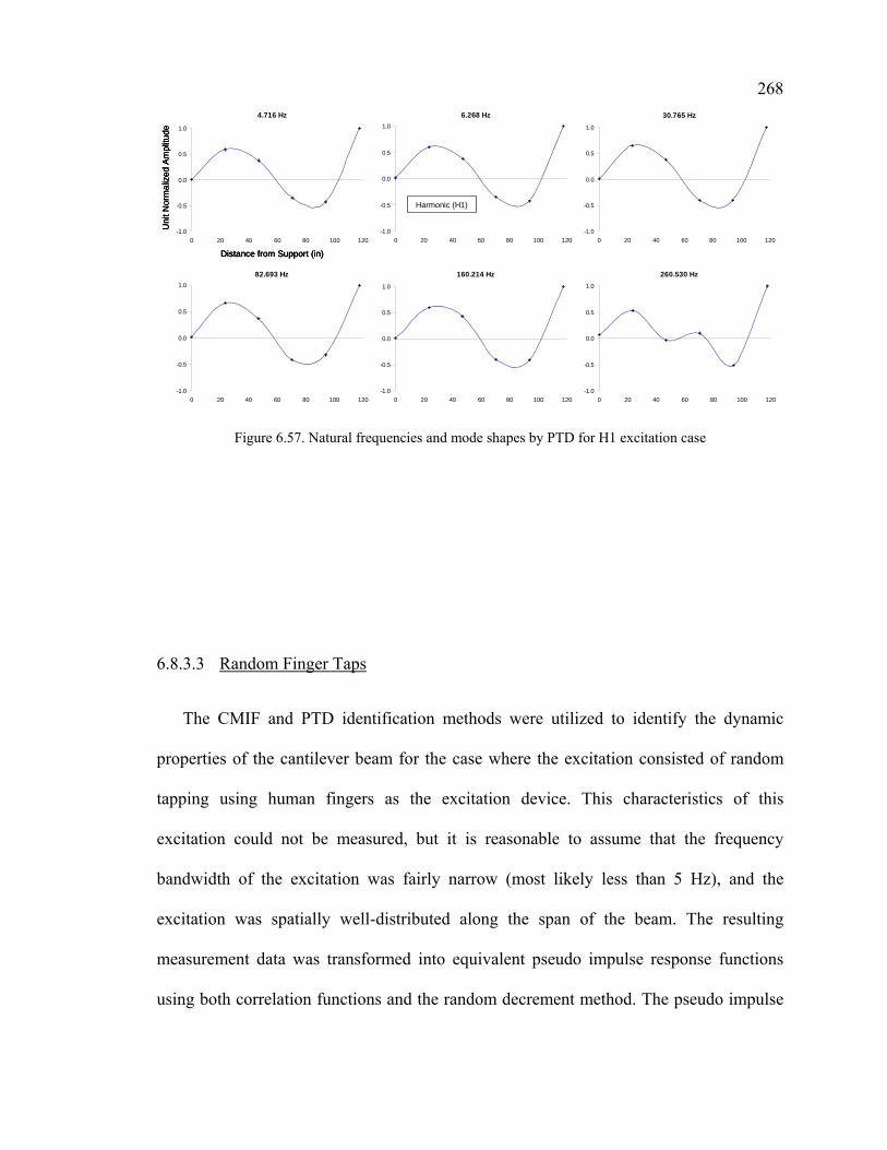
268 4.716 Hz

-1.0

-0.5

0.0

0.5

1.0

0 20 40 60 80 100 120

30.765 Hz

-1.0

-0.5

0.0

0.5

1.0

0 20 40 60 80 100 120

82.693 Hz

-1.0

-0.5

0.0

0.5

1.0

0 20 40 60 80 100 120

6.268 Hz

-1.0

-0.5

0.0

0.5

1.0

0 20 40 60 80 100 120

260.530 Hz

-1.0

-0.5

0.0

0.5

1.0

0 20 40 60 80 100 120

160.214 Hz

-1.0

-0.5

0.0

0.5

1.0

0 20 40 60 80 100 120

Uni

t Nor

mal

ized

Am

plitu

de


Harmonic (H1)

4.716 Hz

-1.0

-0.5

0.0

0.5

1.0

0 20 40 60 80 100 120

30.765 Hz

-1.0

-0.5

0.0

0.5

1.0

0 20 40 60 80 100 120

82.693 Hz

-1.0

-0.5

0.0

0.5

1.0

0 20 40 60 80 100 120

6.268 Hz

-1.0

-0.5

0.0

0.5

1.0

0 20 40 60 80 100 120

260.530 Hz

-1.0

-0.5

0.0

0.5

1.0

0 20 40 60 80 100 120

160.214 Hz

-1.0

-0.5

0.0

0.5

1.0

0 20 40 60 80 100 120

Uni

t Nor

mal

ized

Am

plitu

de


4.716 Hz

-1.0

-0.5

0.0

0.5

1.0

0 20 40 60 80 100 120

30.765 Hz

-1.0

-0.5

0.0

0.5

1.0

0 20 40 60 80 100 120

82.693 Hz

-1.0

-0.5

0.0

0.5

1.0

0 20 40 60 80 100 120

6.268 Hz

-1.0

-0.5

0.0

0.5

1.0

0 20 40 60 80 100 120

260.530 Hz

-1.0

-0.5

0.0

0.5

1.0

0 20 40 60 80 100 120

160.214 Hz

-1.0

-0.5

0.0

0.5

1.0

0 20 40 60 80 100 120

Uni

t Nor

mal

ized

Am

plitu

de


Harmonic (H1)

Figure 6.57. Natural frequencies and mode shapes by PTD for H1 excitation case

6.8.3.3 Random Finger Taps

The CMIF and PTD identification methods were utilized to identify the dynamic

properties of the cantilever beam for the case where the excitation consisted of random

tapping using human fingers as the excitation device. This characteristics of this

excitation could not be measured, but it is reasonable to assume that the frequency

bandwidth of the excitation was fairly narrow (most likely less than 5 Hz), and the

excitation was spatially well-distributed along the span of the beam. The resulting

measurement data was transformed into equivalent pseudo impulse response functions

using both correlation functions and the random decrement method. The pseudo impulse

269 response functions estimated by both methods were used in conjunction with both the

CMIF and PTD methods.

The frequencies and mode shapes identified for this excitation case by the CMIF

method with correlation functions and the random decrement method are shown in Figure

6.58 and Figure 6.59, respectively. The frequencies and mode shapes identified for this

excitation case by the PTD method using correlation functions and the random decrement

method are shown in Figure 6.60 and Figure 6.61, respectively. The final results from

both methods are compared with the theoretical frequencies and mode shapes (using the

MAC parameter) in Table 6.7. It is clear that natural frequencies corresponding to the

five theoretical modes of the cantilever beam are identified by each method. There are

slight variations in the natural frequency values identified from using correlation

functions or random decrement for a given identification method; however, these are

relatively small.

There is significantly more variation in the quality of the mode shapes identified by

each method. The CMIF method with correlation functions produced the most consistent

estimates of the theoretical mode shapes across the entire frequency band as shown by the

MAC values in Table 6.7. The mode shapes identified using the PTD method with

correlation functions and random decrement were much less consistent with their

theoretical counterparts. The results appear to indicate that the CMIF method was

generally less sensitive to the frequency band of the input than the PTD method for

identifying both the natural frequencies and mode shapes provided the excitation was

spatially distributed on the structure. The use of correlation functions also provided mode

shapes that were generally more consistent with their theoretical counterparts for the

270 CMIF and PTD methods. In this study, correlation function estimates were used as the

starting point for the identification by the CMIF and PTD methods to be consistent with

the SSI method.

Table 6.7. Final Identified Frequencies and MAC Values: Random Finger Taps Excitation Case

Excitation Case: RFT CMIF

(Corr. Functions) CMIF

(Random Decrement) PTD

(Corr. Functions) PTD

(Random Decrement)

Mode Freq. (Hz)

Freq Diff (%)1 MAC2

Freq. (Hz)

Freq Diff (%)1 MAC2

Freq. (Hz)

Freq Diff (%)1 MAC2

Freq. (Hz)

Freq Diff (%)1 MAC2

1 4.702 -4.2 1.000 4.700 -4.3 1.000 4.781 -2.6 1.000 4.763 -3.0 0.991 2 29.430 -4.4 0.923 29.194 -5.1 0.957 29.773 -3.2 0.480 29.485 -4.2 0.944 3 83.293 -3.3 0.995 83.068 -3.6 0.948 83.305 -3.3 0.712 83.345 -3.3 0.371 4 162.094 -4.0 0.993 161.788 -4.2 0.447 162.118 -4.0 0.873 162.121 -4.0 0.031 5 263.237 -5.7 0.998 263.089 -5.7 0.958 263.263 -5.7 0.366 263.298 -5.7 0.321

1. Compared with theoretical natural frequency 2. Compared with theoretical mode shape

4.702 Hz

-1.0

-0.5

0.0

0.5

1.0

0 20 40 60 80 100 120

29.430 Hz

-1.0

-0.5

0.0

0.5

1.0

0 20 40 60 80 100 120

83.293 Hz

-1.0

-0.5

0.0

0.5

1.0

0 20 40 60 80 100 120

162.094 Hz

-1.0

-0.5

0.0

0.5

1.0

0 20 40 60 80 100 120

263.237 Hz

-1.0

-0.5

0.0

0.5

1.0

0 20 40 60 80 100 120

Uni

t Nor

mal

ized

Am

plitu

de


4.702 Hz

-1.0

-0.5

0.0

0.5

1.0

0 20 40 60 80 100 120

29.430 Hz

-1.0

-0.5

0.0

0.5

1.0

0 20 40 60 80 100 120

83.293 Hz

-1.0

-0.5

0.0

0.5

1.0

0 20 40 60 80 100 120

162.094 Hz

-1.0

-0.5

0.0

0.5

1.0

0 20 40 60 80 100 120

263.237 Hz

-1.0

-0.5

0.0

0.5

1.0

0 20 40 60 80 100 120

Uni

t Nor

mal

ized

Am

plitu

de


Figure 6.58. Natural frequencies and mode shapes by CMIF using correlation functions for random finger taps excitation case

271 4.700 Hz

-1.0

-0.5

0.0

0.5

1.0

0 20 40 60 80 100 120

29.194 Hz

-1.0

-0.5

0.0

0.5

1.0

0 20 40 60 80 100 120

83.068 Hz

-1.0

-0.5

0.0

0.5

1.0

0 20 40 60 80 100 120

161.788 Hz

-1.0

-0.5

0.0

0.5

1.0

0 20 40 60 80 100 120

263.089 Hz

-1.0

-0.5

0.0

0.5

1.0

0 20 40 60 80 100 120

Uni

t Nor

mal

ized

Am

plitu

de


4.700 Hz

-1.0

-0.5

0.0

0.5

1.0

0 20 40 60 80 100 120

29.194 Hz

-1.0

-0.5

0.0

0.5

1.0

0 20 40 60 80 100 120

83.068 Hz

-1.0

-0.5

0.0

0.5

1.0

0 20 40 60 80 100 120

161.788 Hz

-1.0

-0.5

0.0

0.5

1.0

0 20 40 60 80 100 120

263.089 Hz

-1.0

-0.5

0.0

0.5

1.0

0 20 40 60 80 100 120

Uni

t Nor

mal

ized

Am

plitu

de


Figure 6.59. Natural frequencies and mode shapes by CMIF using random decrement for random finger taps excitation case

4.781 Hz

-1.0

-0.5

0.0

0.5

1.0

0 20 40 60 80 100 120

29.773 Hz

-1.0

-0.5

0.0

0.5

1.0

0 20 40 60 80 100 120

83.305 Hz

-1.0

-0.5

0.0

0.5

1.0

0 20 40 60 80 100 120

162.118 Hz

-1.0

-0.5

0.0

0.5

1.0

0 20 40 60 80 100 120

263.263 Hz

-1.0

-0.5

0.0

0.5

1.0

0 20 40 60 80 100 120

Uni

t Nor

mal

ized

Am

plitu

de


4.781 Hz

-1.0

-0.5

0.0

0.5

1.0

0 20 40 60 80 100 120

29.773 Hz

-1.0

-0.5

0.0

0.5

1.0

0 20 40 60 80 100 120

83.305 Hz

-1.0

-0.5

0.0

0.5

1.0

0 20 40 60 80 100 120

162.118 Hz

-1.0

-0.5

0.0

0.5

1.0

0 20 40 60 80 100 120

263.263 Hz

-1.0

-0.5

0.0

0.5

1.0

0 20 40 60 80 100 120

Uni

t Nor

mal

ized

Am

plitu

de


Figure 6.60. Natural frequencies and mode shapes by PTD using correlation functions for random finger taps excitation case

272 4.763 Hz

-1.0

-0.5

0.0

0.5

1.0

0 20 40 60 80 100 120

29.485 Hz

-1.0

-0.5

0.0

0.5

1.0

0 20 40 60 80 100 120

83.345 Hz

-1.0

-0.5

0.0

0.5

1.0

0 20 40 60 80 100 120

162.121 Hz

-1.0

-0.5

0.0

0.5

1.0

0 20 40 60 80 100 120

263.298 Hz

-1.0

-0.5

0.0

0.5

1.0

0 20 40 60 80 100 120

Uni

t Nor

mal

ized

Am

plitu

de


4.763 Hz

-1.0

-0.5

0.0

0.5

1.0

0 20 40 60 80 100 120

29.485 Hz

-1.0

-0.5

0.0

0.5

1.0

0 20 40 60 80 100 120

83.345 Hz

-1.0

-0.5

0.0

0.5

1.0

0 20 40 60 80 100 120

162.121 Hz

-1.0

-0.5

0.0

0.5

1.0

0 20 40 60 80 100 120

263.298 Hz

-1.0

-0.5

0.0

0.5

1.0

0 20 40 60 80 100 120

Uni

t Nor

mal

ized

Am

plitu

de


Figure 6.61. Natural frequencies and mode shapes by PTD using random decrement for random finger taps excitation case

6.8.3.4 MIMO Impact Test

The identification results from a MIMO impact test conducted on the cantilever beam

are summarized in Table 6.8. These results may serve as an additional baseline for the

experimental characterization of the cantilever beam. There are slight differences in the

frequencies identified by the CMIF and PTD methods, but the experimentally identified

frequencies are generally slightly smaller than the theoretical frequencies. Indeed, the

experimental frequencies identified in the previous excitation cases are generally more

consistent with the experimental frequencies from the impact test than with the

theoretical natural frequencies. This is a reasonable result as the different experimental

characterizations will often reflect the actual characteristics of the structure better than a

purely theoretical or analytical characterization. The mode shapes identified from this test

by the CMIF and PTD methods were also significantly more consistent with the

273 theoretical mode shapes for the cantilever beam than in the other excitation cases where

these methods were applied.

The dynamic properties (natural frequencies and mode shapes) identified by both the

CMIF and PTD methods were consistent with the expected theoretical results for the

cantilever beam. This was generally not the case for the other excitation cases evaluated

in this study. This observation tends to indicate that these two identification methods are

very sensitive to the quality and the character of the supplied excitation. The excitation

supplied in the MIMO impact test may be characterized as a broadband impulse with a

flat spectrum over the frequency range. Furthermore, this excitation is provided directly

on the structure at each measurement degree of freedom. The high quality (good signal-

to-noise level) dynamic excitation that is directly applied in a consistent manner to each

of the measurement degrees of freedom on the structure represents an ideal set of

excitation characteristics for the experimental characterization of the cantilever beam’s

dynamic properties. The MIMO impact test demonstrates that the CMIF and PTD

methods will correctly identify the natural frequencies and mode shapes of the cantilever

beam for ideal dynamic excitation conditions.

Table 6.8. Experimental frequencies and mode shapes from multiple reference impact test

Impact Test (PTD) Impact Test (CMIF)

Mode

Theor. Freq. (Hz)

Freq. (Hz)

Freq. Diff (%)1 MAC2

Freq. (Hz)

Freq. Diff (%)1 MAC2

1 4.910 4.726 -3.7 1.000 4.684 -4.6 1.000 2 30.770 29.619 -3.7 0.996 29.570 -3.9 0.997 3 86.157 83.214 -3.4 0.995 83.146 -3.5 0.996 4 168.846 161.678 -4.2 0.992 161.622 -4.3 0.993 5 279.091 262.990 -5.8 0.994 262.818 -5.8 0.995 1. Compared with theoretical natural frequency 2. Compared with theoretical mode shape

274 6.9 Discussion

In this study, the influence of the character of the ambient dynamic excitation has on

the reliability of the identified modal properties was evaluated for a simple and

mechanically transparent laboratory structure. The different excitation cases that were

evaluated in this study were designed based on a subjective characterization of the nature

of direct and transmitted ambient dynamic excitation for the towers of a suspension

bridge. The primary excitation characteristics that were considered included the effective

bandwidth of random dynamic excitation, and random dynamic excitation with different

effective frequency bandwidths that contained a harmonic excitation component. The

supplied dynamic excitation was controlled for each excitation case that was considered,

but was treated as unmeasured ambient dynamic excitation for the purpose of identifying

the dynamic properties of the test structure. The external excitation was transmitted to the

structure through the clamped support. The study also included a narrow band random

excitation that was applied directly to the cantilever as an addition evaluation case.

Finally, a multiple-reference impact test was conducted to serve as an additional baseline

experimental characterization for the cantilever beam.

The different excitation characteristics applied in each case were used to compare and

evaluate the effectiveness of different modal identification methods for complex ambient

dynamic excitation characteristics that may be expected to occur in the case of cable

supported structures. The identification methods evaluated included the Peak Picking

(PP) method, the Stochastic Subspace Identification (SSI) method, the Complex Mode

Indicator Function (CMIF) method, and the Polyreference Time Domain (PTD) method.

The classical single reference sensor approach commonly used for PP in ambient

275 vibration tests was modified to incorporate the multiple reference sensors available when

a stationary instrumentation scheme is utilized, and an automated identification procedure

was developed for use with this method.

The natural frequencies and MAC values for the mode shapes identified by the PP,

SSI, CMIF and PTD methods for the BB400, BB400+H1, NB200 and NB200+H1

excitation cases are summarized in Table 6.9. The same values are summarized for the

NB50, NB50+H1, NB10, and NB10+H1 excitation cases in Table 6.10. The results from

the H1 excitation case are given in Table 6.11. Results that are considered poor are

shown in bold. It is clear from these results that the characteristics of the applied dynamic

excitation did not have a significant effect on the identification results. The first four

natural frequencies and mode shapes of the beam were identified by PP in all of the pure

random excitation cases, and the fifth natural frequency could only be identified from the

first pure random excitation case (BB400). All five natural frequencies could be

identified from all of the random excitation cases that included a harmonic excitation

component. It is apparent that there was enough excitation energy available at the higher

frequencies of the cantilever beam to permit these modes to be identified. There was

some variation in the frequencies identified at the higher modes in some of the narrow

band excitation cases, but the observed variations were not very significant.

6.9.1 Identification Methods

6.9.1.1 Peak Picking (PP) Method

The automated PP procedure developed and used in conjunction with this study

compared the effectiveness an existing ANPSD mode indicator function (MIF) with two

276 additional MIFS for each excitation case. The additional MIFs utilized included the

SPSD function which may be considered a simpler variation of the ANPSD function

since it does not utilize any normalization or averaging of the diagonal elements of the

spectral density matrix. The other MIF developed and evaluated for the PP method used

in this study was termed the SSCSD function, which combined multiple rows or columns

of the spectral density matrix corresponding the number of sensors selected to serve as

references.

The results indicated that there were no significant differences between the numbers

of spectral peaks identified by each MIF when an automated peak detection procedure

was used. The automated peak identification procedure that was developed and used to

identify the spectral peaks in each MIF compared the amplitude of the MIF at each

spectral line with its value at different numbers adjacent spectral lines. The spectral peaks

identified using this approach included the natural frequencies of the cantilever beam,

any peaks in the excitation spectrum, and various quantities of spurious peaks that were

related to noise and other experimental and signal processing errors. Identifying the

spectral peaks that correspond to the natural frequencies from the population of spectral

peaks identified by the automated procedure is the primary challenge with this method.

The numbers of peaks identified by the automated procedure could be decreased without

losing the natural frequencies by using a more considering the amplitude of the MIF at

larger numbers of spectral peaks. In this study, the peaks were identified by comparing

the MIF value at each spectral line with its value at the four adjacent spectral lines before

and after the spectral line under consideration. This criterion produced a reasonable

277 number of identified spectral peaks for subsequent evaluation, without filtering out any of

the natural frequencies.

A minimum amplitude level threshold value criterion was also applied to the spectral

peaks after their initial identification. The use of a level threshold increased the efficiency

of the PP identification with the SPSD and SSCSD functions as compared to the ANPSD

function. The efficiency was evaluated based on the number of spurious peaks remaining

in the identified spectral peak population for each MIF. This illustrated that the

normalization applied for the computation of the ANPSD can actually be

counterproductive since it brings spurious peaks and low-level responses to a level that is

more consistent with the high signal-to-noise peaks associated with the natural

frequencies of the structure. The spurious results cannot be effectively removed by a level

threshold value as with the non-normalized SPSD and SSCSD functions.

The SSCSD function incorporated multiple rows or columns of the spectral density

matrix into the MIF for identifying the spectral peaks. This did not yield any significant

difference in the identified results. This should have been expected; however, since a

multiple reference approach is most beneficial for structures with closely spaced modes,

or when the reference sensors are located at nodal points of the structure. Since neither of

these conditions was applicable to the cantilever beam, the SSCSD results were

consistent with the other MIFs. The SSCSD function should be evaluated in the future to

test its effectiveness under these specific conditions.

The automated PP procedure developed and implemented for this study provided the

most consistent identification results for all of the excitation cases evaluated. The

procedure as implemented is very transparent, allowing the data analyst to retain a

278 physical sense of the results at each stage of the identification. The computation of mode

shapes for multiple reference sensors enables the frequency bandwidth of the unmeasured

excitation to be evaluated along with the corresponding reliability of the identified results

based on simple visual evaluation of the results. The PP procedure used consistently

identified the most reliable results for each excitation case, and the additional coherence

and MAC parameters computed with this method provided additional information that

can be used to evaluate the reliability of the identified results. The spectral peaks

corresponding to the known harmonic excitation could also be effectively identified and

excluded from the identification results.

6.9.1.2 Advanced Identification Methods

The SSI method was superior to the CMIF and PTD methods for accurately

identifying the natural frequencies and mode shapes for the excitation cases that were

evaluated. The CMIF and PTD methods were particularly sensitive to the excitation

characteristics, and performed much better at identifying the frequencies than the mode

shapes. All of the advanced identification methods identified frequencies and mode

shapes corresponding to spurious modes and harmonics in the excitation spectrum. Since

much of the identification steps occur in the background with these methods, it was very

difficult to exclude these from the final results without using the theoretical results or the

results from the PP identification as a guide. The various criteria customarily used to

exclude spurious results with these methods (model order, stability plots, damping, and

animated mode shapes) did not indicate that many of the spurious results should be ruled

out. This was especially true with the SSI method since many of the spurious results

279 appeared quite reasonable and would not be automatically excluded. In the case of the

CMIF and PTD methods, most of the natural frequencies would be ruled out with any

spurious results since the identified mode shapes were generally poor in the excitation

cases that were evaluated. The SSI method also identified natural frequencies and mode

shapes that were determined to be unreliable with good justification in the PP method.

The comparisons conducted in this study demonstrate that the PP method can perform

quite reasonably in ambient vibration tests where the excitation is complex. Furthermore,

the PP approach provided results that were generally more consistent and reliable than

the advanced identification methods used, and the identification and interpretation

process was significantly more transparent. This would indicate that the advanced

identification methods utilized in this study may only really be more effective for very

specific structural configurations (such as with closely-spaced modes or repeated roots);

however, the parameters created for the PP approach may still be necessary in these cases

to aid in the interpretation of the results. It should also be noted that the structural

configuration of the towers and pylons in cable-supported bridges will generally not lead

to closely-spaced modes or repeated roots.

280 Table 6.9. Final Identified Frequencies and MAC Values: BB400 & NB200 Excitation Cases

Excitation Case: BB400

Peak Pick SSI CMIF PTD

Mode Freq. (Hz)

Freq Diff (%)1 MAC2

Freq. (Hz)

Freq Diff (%)1 MAC2

Freq. (Hz)

Freq Diff (%)1 MAC2

Freq. (Hz)

Freq Diff (%)1 MAC2

1 4.688 -4.5 1.000 4.735 -3.6 1.000 4.659 -5.1 1.000 4.737 -3.5 0.995 2 29.297 -4.8 0.997 29.449 -4.3 0.997 29.500 -4.1 0.995 29.633 -3.7 0.986 3 82.617 -4.1 0.995 82.742 -4.0 0.991 83.707 -2.8 0.085 82.748 -4.0 0.185 4 160.840 -4.7 0.992 160.880 -4.7 0.993 163.786 -3.0 0.165 160.881 -4.7 0.204 5 260.938 -6.5 0.993 240.040 -6.5 0.989 261.221 -6.4 0.699 260.819 -6.5 0.187

Excitation Case: BB400+H1


Mode Freq. (Hz)

Freq Diff (%)1 MAC2

Freq. (Hz)

Freq Diff (%)1 MAC2

Freq. (Hz)

Freq Diff (%)1 MAC2

Freq. (Hz)

Freq Diff (%)1 MAC2

1 4.688 -4.5 1.000 4.732 -3.6 1.000 4.544 -7.5 0.921 4.720 -3.9 0.134 2 29.785 -3.2 0.998 29.849 -3.0 0.998 NA NA NA 31.567 2.6 0.162 3 82.715 -4.0 0.996 82.753 -4.0 0.996 82.686 -4.0 0.778 82.460 -4.3 0.993 4 160.449 -5.0 0.991 160.260 -5.1 0.992 166.533 -1.4 0.161 160.244 -5.1 0.168 5 260.449 -6.7 0.993 260.500 -6.7 0.993 NA NA NA 260.551 -6.6 0.681

Excitation Case: NB200


Mode Freq. (Hz)

Freq Diff (%)1 MAC2

Freq. (Hz)

Freq Diff (%)1 MAC2

Freq. (Hz)

Freq Diff (%)1 MAC2

Freq. (Hz)

Freq Diff (%)1 MAC2

1 4.688 -4.5 1.000 4.726 -3.7 1.000 4.654 -5.2 1.000 4.727 -3.7 0.999 2 29.785 -3.2 0.998 29.144 -5.3 0.998 29.555 -3.9 0.994 29.502 -4.1 0.842 3 82.813 -3.9 0.996 82.973 -3.7 0.999 82.983 -3.7 0.145 83.042 -3.6 0.154 4 160.156 -5.1 0.990 160.200 -5.1 0.792 146.680 -13 0.200 160.250 -5.1 0.183 5 NA NA NA 260.580 -6.6 0.953 NA NA NA 260.539 -6.6 0.160

Excitation Case: NB200+H1


Mode Freq. (Hz)

Freq Diff (%)1 MAC2

Freq. (Hz)

Freq Diff (%)1 MAC2

Freq. (Hz)

Freq Diff (%)1 MAC2

Freq. (Hz)

Freq Diff (%)1 MAC2

1 4.688 -4.5 1.000 4.725 -3.8 1.000 NA NA NA 4.723 -3.8 0.137 2 29.785 -3.2 0.998 29.089 -5.5 0.997 NA NA NA 29.510 -4.1 0.192 3 82.715 -4.0 0.995 82.788 -3.9 0.999 82.721 -4.0 0.902 82.824 -3.9 0.886 4 160.156 -5.1 0.991 160.230 -5.1 0.995 165.328 -2.1 0.181 160.195 -5.1 0.185 5 260.547 -6.6 0.992 260.550 -6.6 0.980 NA NA NA 260.577 -6.6 0.240


281 Table 6.10. Final Identified Frequencies and MAC Values: NB50 & NB10 Excitation Cases



Mode Freq. (Hz)

Freq Diff (%)1 MAC2

Freq. (Hz)

Freq Diff (%)1 MAC2

Freq. (Hz)

Freq Diff (%)1 MAC2

Freq. (Hz)

Freq Diff (%)1 MAC2

1 4.785 -2.5 1.000 4.740 -3.5 1.000 4.667 -4.9 1.000 4.747 -3.3 0.999 2 29.395 -4.5 0.997 29.376 -4.5 0.997 29.529 -4.0 0.997 29.492 -4.2 0.622 3 82.617 -4.1 0.995 82.757 -3.9 0.989 83.178 -3.5 0.684 82.757 -3.9 0.173 4 161.035 -4.6 0.992 160.990 -4.7 0.993 NA NA NA 160.888 -4.7 0.207 5 NA NA NA 261.120 -6.4 0.993 NA NA NA 261.098 -6.4 0.196



Mode Freq. (Hz)

Freq Diff (%)1 MAC2

Freq. (Hz)

Freq Diff (%)1 MAC2

Freq. (Hz)

Freq Diff (%)1 MAC2

Freq. (Hz)

Freq Diff (%)1 MAC2

1 4.688 -4.5 1.000 4.722 -3.8 1.000 NA NA NA 4.713 -4.0 0.135 2 29.785 -3.2 0.998 29.634 -3.7 0.998 NA NA NA 29.118 -5.4 0.175 3 82.617 -4.1 0.995 82.758 -3.9 0.998 82.627 -4.1 0.999 82.766 -3.9 0.874 4 160.254 -5.1 0.991 160.240 -5.1 0.995 168.595 -0.1 0.792 160.167 -5.1 0.185 5 260.449 -6.7 0.991 260.620 -6.6 0.990 NA NA NA 260.490 -6.7 0.245



Mode Freq. (Hz)

Freq Diff (%)1 MAC2

Freq. (Hz)

Freq Diff (%)1 MAC2

Freq. (Hz)

Freq Diff (%)1 MAC2

Freq. (Hz)

Freq Diff (%)1 MAC2

1 4.785 -2.5 1.000 4.773 -2.8 0.933 4.669 -4.9 1.000 4.747 -3.3 0.999 2 29.395 -4.5 0.997 29.112 -5.4 0.688 29.503 -4.1 0.997 29.465 -4.2 0.340 3 82.617 -4.1 0.995 82.667 -4.1 0.995 83.765 -2.8 0.017 82.695 -4.0 0.153 4 160.938 -4.7 0.992 160.250 -5.1 0.989 NA NA NA 160.912 -4.7 0.163 5 NA NA NA 260.680 -6.6 0.045 NA NA NA 261.083 -6.5 0.165



Mode Freq. (Hz)

Freq Diff (%)1 MAC2

Freq. (Hz)

Freq Diff (%)1 MAC2

Freq. (Hz)

Freq Diff (%)1 MAC2

Freq. (Hz)

Freq Diff (%)1 MAC2

1 4.688 -4.5 1.000 4.722 -3.8 1.000 4.544 -7.5 0.921 4.712 -4.0 0.143 2 29.492 -4.2 0.998 29.634 -3.7 0.998 NA NA NA NA NA NA 3 82.715 -4.0 0.995 82.758 -3.9 0.998 82.686 -4.0 0.993 82.797 -3.9 0.896 4 160.254 -5.1 0.991 160.240 -5.1 0.995 166.533 -1.4 0.112 160.195 -5.1 0.187 5 260.449 -6.7 0.992 260.620 -6.6 0.990 NA NA NA 260.530 -6.7 0.254


282 Table 6.11. Final Identified Frequencies and MAC Values: H1 Excitation Case

Excitation Case: H1


Mode Freq. (Hz)

Freq Diff (%)1 MAC2

Freq. (Hz)

Freq Diff (%)1 MAC2

Freq. (Hz)

Freq Diff (%)1 MAC2

Freq. (Hz)

Freq Diff (%)1 MAC2

1 4.688 -4.5 1.000 4.727 -3.7 0.993 NA NA NA 4.716 -4.0 0.155 2 29.688 -3.5 0.998 29.505 -4.1 0.976 NA NA NA 30.765 0.0 0.139 3 82.715 -4.0 0.996 82.734 -4.0 0.995 82.686 -4.0 0.016 82.693 -4.0 0.981 4 160.254 -5.1 0.991 160.260 -5.1 0.990 161.283 -4.5 0.993 160.214 -5.1 0.160 5 260.449 -6.7 0.993 260.550 -6.6 0.991 260.374 -6.7 0.989 260.530 -6.7 0.686


283 CHAPTER 7: RIGOROUS MODAL IDENTIFICATION OF

THE BROOKLYN BRIDGE TOWERS

7.1 Introduction

This chapter compares the identification of the modal properties for the ambient

vibration data from the Brooklyn Bridge towers using several different modal parameter

identification methods. The modal parameter identification methods that were used and

evaluated in this study were essentially the same methods that were previously compared

in Chapter 6 for the cantilever beam in the laboratory. Specifically, the identification

methods that were applied to the ambient vibration data from the Brooklyn Bridge

included the modified version of the basic peak-picking (PP) method described in

Chapter 6, the Stochastic Subspace Identification (SSI) method, the Polyreference Time

Domain (PTD) method, and the Complex Mode Indicator Function (CMIF) method.

There were several objectives for applying and evaluating the effectiveness of these

different identification methods for the Brooklyn Bridge ambient vibration data.

One objective of this study was to compare the modal identification results obtained

by the multiple-reference extension to the basic peak-picking identification method with

those obtained from the most basic implementation of the peak-picking method for a

single reference location. The former method may be used for ambient vibration test data

acquired using a stationary instrumentation scheme while the latter method represents the

more common implementation of the peak-picking method for ambient vibration test data

acquired by a roving instrumentation scheme. The most basic implementation of the

peak-picking method was previously applied to the same data set in Chapter 4 to identify

the natural frequencies and mode shapes for the Brooklyn Tower assuming that the

284 accelerometers that were installed just above the roadway deck level on the Brooklyn

Tower (Level E) were the only sensors that remained stationary during the ambient

vibration test. In this case, the accelerometers located at Level E served as the only

reference sensors for the identification of the modal properties. The actual ambient

vibration test of the Brooklyn Bridge employed a stationary instrumentation scheme in

which all of the accelerometers locations on the towers and the spans remained constant

and were simultaneously sampled throughout the testing. In the present study, all

accelerometer locations on the bridge may serve as reference locations for the purpose of

identifying the modal properties of the Brooklyn Tower. It is therefore possible to

evaluate if the resulting identification of the modal properties of the Brooklyn Tower may

be enhanced by incorporating the additional reference locations.

A related objective was to evaluate how the sensor locations from the other locations

on the bridge, namely the two measurement stations in the main and side spans near the

Brooklyn Tower and the single measurement level on the Manhattan Tower, could be

used in conjunction with the identification of the modal properties for the Brooklyn

Tower. The accelerometers located on these other bridge components were also

stationary throughout the ambient vibration testing and were simultaneously measured

with the accelerometers located on the Brooklyn Tower. Although these additional

accelerometer locations were not sufficient for identifying the modal properties of the

spans and Manhattan Tower, they may provide sufficient information regarding the local

and global responses of the bridge when they are considered in conjunction with the

experimental characterization of the spans that was conducted in conjunction with the

pedestrian induced vibrations investigation (Kulczycki et al., 2004; Hodgson, Connor and

285 Bowman, 2004). In Chapter 5, it was shown that the Brooklyn Bridge may be considered

to behave as a weakly-coupled dynamic system, and the ambient vibration measurements

and modal identification results for the spans may therefore prove critical for reliably

identifying the modal properties for the Brooklyn Tower.

A final objective of this study is to compare the effectiveness of some common modal

parameter identification methods for a real life application in which the structure being

evaluated (the Brooklyn Tower) represents one subcomponent of a weakly-coupled

dynamic system. The comparative evaluation of these different methods in the laboratory

that was discussed in Chapter 6 simulated the uncertainty related to the ambient dynamic

excitation environment for the towers in a cable-supported bridge structure; however,

there is still merit in conducting a similar evaluation for ambient vibration data acquired

from Brooklyn Bridge. In particular, the dynamic interactions of the spans and towers

were simulated through the definition of complex ambient dynamic excitation cases that

were applied to the cantilever beam in Chapter 6.

The complex excitation cases were designed on the basis of a qualitative

characterization of the ambient dynamic excitation environment for the tower

components in cable-supported bridges. The ambient vibration measurements from the

Brooklyn Bridge contain various sources of experimental uncertainty and reflect the

effects of dynamic interactions between the stiff and flexible subcomponents of a weakly-

coupled dynamic system. A comparative evaluation of the different modal parameter

identification methods may be performed with greater confidence for the subcomponents

of an in-service structure with weakly-coupled dynamic system characteristics based on

the observations made from the previous evaluation with the mechanically transparent

286 laboratory specimen. Furthermore, a comparative evaluation of these same identification

methods for the ambient vibration measurements from the Brooklyn Bridge may also

provide additional corroboration of the observations made for the cantilever beam

specimen.

It should be noted that that the ambient dynamic excitation levels provided to the

cantilever beam specimen and it corresponding vibration response amplitudes were

somewhat larger than the corresponding ambient vibration amplitudes that were observed

for the various subcomponents of the Brooklyn Bridge described in Chapter 4. The actual

ambient vibration measurements from the Brooklyn Bridge represent a more accurate

reflection of the ambient vibration response levels which may be encountered for the

principal structural subcomponents in a cable-supported bridge, and a comparative

evaluation of the different modal identification methods for this data may be expected to

have slightly better correspondence to a greater range of in-service cable-supported

bridge structures with similar structural and excitation characteristics.

7.2 Scope

In the following sections of this chapter, the modal properties (natural frequencies

and mode shapes) of the Brooklyn Tower determined by several different modal

parameter identification methods are presented and compared. The reader should refer to

Chapter 4 for the details of the Brooklyn Bridge and the experimental setup used for the

ambient vibration test, and to Chapter 6 for additional background and details of the

computations employed for the multiple-reference extension to the basic peak-picking

procedure that is utilized for this study.

287 The ambient vibration measurements of the Brooklyn Tower in the longitudinal,

torsional, and lateral response directions were evaluated using the following modal

parameter identification methods to determine the natural frequencies and the

corresponding mode shapes:

• Peak-Picking

• SSI Method

• PTD Method

• CMIF Method

In the peak-picking method used for this study, the locations of spectral peaks in the

frequency spectra of the vibrations of the Brooklyn Tower in the longitudinal, torsional

and lateral response directions using the automated peak identification procedure with

different mode indicator functions (MIFs) as was previously outlined in Chapter 4. The

automated spectral peak identification procedure is also employed for the more limited

instrumentation that was deployed on the flexible spans near the Brooklyn Tower and on

the Manhattan Tower. The results of the previous experimental characterization of the

spans by ambient vibration and forced-vibration testing are also noted and considered for

interpreting the spectral peaks identified for the current span measurements. Additional

parameters derived from the computation of the ordinary coherence function between an

output sensor location and a selected reference output sensor location are also computed

and evaluated for the accelerometers on Brooklyn Tower, the main (river) and side (land)

spans near the Brooklyn Tower, and the Manhattan Tower. Parameters based on the

computation of the modal assurance criterion (MAC) are also computed from the

288 measurements from the Brooklyn Tower and considered in the evaluation of the natural

frequencies and mode shapes for the tower.

The Stochastic Subspace Identification (SSI) method is also used to identify the

natural frequencies and mode shapes for the Brooklyn Tower in the longitudinal,

torsional, and lateral response directions. The ambient vibration data was analyzed with

this method using the commercially available program LMS TestLab. The SSI method,

termed the Time MDOF approach in the LMS TestLab (Version 6) software package, can

utilize multiple references. In this study, all of the accelerometers on the Brooklyn Tower

in a given response direction (longitudinal, torsional, or lateral) were selected as

reference sensors for the identification of the modal properties.

The ambient vibration measurements from Brooklyn Tower were also evaluated using

the Polyreference Time Domain (PTD) method and the Complex Mode Indicator

Function (CMIF) method. The former method identifies the modal properties from time

domain data while the latter method performs the identification in the frequency domain.

The data were analyzed using these methods with the program X-Modal II from the

Structural Dynamics Research Laboratory (SDRL) at the University of Cincinnati. Both

of these methods can utilize multiple reference sensors for the identification of the modal

properties. As was the case with the SSI method, all of the accelerometers on the

Brooklyn Tower in a given response direction were selected as reference sensors for the

identification of the modal properties using the PTD and CMIF methods.

289 7.3 Data Processing

The pre-processing procedures (data cleaning, data filtering, and the decoupling of

the 3D vibration responses) employed for the data evaluated in this chapter are the same

as those which were described in Chapter 4 for the initial evaluation of the Brooklyn

Bridge ambient vibration data. The additional data processing procedures employed for

the different modal parameter identification methods utilized in this study are described

in the following sections.

7.3.1 Peak-Picking (PP)

7.3.1.1 Estimation of Spectral Densities

The starting point for the identification of the modal properties by PP was to estimate

the full spectral matrix from the output measurements. The elements of the full spectral

matrix are the autospectral densities (the diagonal terms of the spectral matrix) and the

magnitudes of the complex cross power spectral densities (the off-diagonal terms of the

spectral matrix). One row or column of the spectral matrix is estimated for each reference

location selected. In the case of the Brooklyn Tower, the full spectral matrix estimated for

the decoupled longitudinal vibration responses included five references (Levels B, C, E,

G, and H on the Brooklyn Tower). The full spectral matrix estimated for the decoupled

torsional vibration response of the Brooklyn Tower also included five references from the

same levels as the longitudinal responses. The longitudinal and torsional vibration

responses at Level F were not used as references since one of the accelerometers at this

level did not function during the vibration testing.

290 A total of three separate spectral matrices were estimated for the lateral responses of

the Brooklyn Tower, with one corresponding to each of the north, middle and south tower

columns above the roadway deck level. Each spectral matrix for the lateral responses of

the tower included six reference levels (Level B, C, E, F, G, and H on the Brooklyn

Tower). The lateral accelerometer that served as the reference sensor at Level B, C, E,

and H was the same in each spectral matrix, and a different lateral accelerometer was

used for the reference at Level F and G (north, middle and south columns) in each of the

three spectral matrices that were estimated for the lateral vibration responses of the

Brooklyn Tower. The measurement levels on the Brooklyn Tower were described in

Chapter 4, and are shown once more in Figure 7.1.

The autospectral densities (ASD) and cross spectral densities (CSD) corresponding to

each reference location in a given tower vibration response direction (longitudinal,

torsional, and lateral) were estimated by Welch’s average modified periodogram method.

The procedure and equations used to compute the ASD and CSD estimates using this

method were described in Chapter 6. The resulting frequency resolution for the ASD and

CSD estimates was 0.0049 Hz.

291


(L = Longitudinal Accelerometer, T = Transverse Accelerometer)52

’33

’39

’54

’54

’40

.5’

272.

5’

TLL

TLTLTL

TLTLTL

TLL

TLL

TLL Longitudinal, Torsional, Lateral

Longitudinal, Torsional, Lateral




Lateral

Vibration Response at Each Level



’33

’39

’54

’54

’40

.5’

272.

5’

TLL

TLTLTL

TLTLTL

TLL

TLL

TLL



’33

’39

’54

’54

’40

.5’

272.

5’

TLL

TLTLTL

TLTLTL

TLL

TLL

TLL

52’

33’

39’

54’

54’

40.5

’

272.

5’

TL TTLLLL



TL TTLLLL

TL TTLLLL

TL TTLLLL Longitudinal, Torsional, Lateral





Lateral

Vibration Response at Each Level

Figure 7.1. Vibration responses at each level on Brooklyn Tower

7.3.1.2 Identification of Modal Parameters

The auto and cross-spectral densities served as the starting point for the PP

identification procedure. A separate parameter matrix was constructed for each vibration

response direction of the Brooklyn Tower (longitudinal, torsional and lateral). Each

parameter matrix included columns corresponding to three different mode indicator

functions (MIFs), normalized mode shapes (operating deflection shapes) computed using

each reference response, and ordinary coherence function values computed using each

reference response. The computed mode shapes were forced to have normal mode

characteristics by using a whitewashing procedure on the phase factor values computed

292 from each CSD. A separate set of mode shapes was computed using each output response

on the Brooklyn Tower as a reference response.

The different MIFs used for this study were the ANPSD, the SPSD and the SSCSD

functions which were detailed in Chapter 6. The peaks in each MIF were identified in an

automated fashion by comparing the MIF value at every frequency line with the MIF

value at a set number of contiguous frequency lines immediately before and after it. If the

MIF value at a given frequency line was larger than its value at the predetermined

number of frequency lines before and after it, it was identified as a peak location. A total

of three different numbers of contiguous frequency line criteria (3 points, 4 points and 5

points) were utilized for comparison purposes. These three different criteria were referred

to as the 3P, 4P and 5P identification criteria. A minimum amplitude threshold level for

the MIF values was also specified and used as an additional criterion for identifying the

peaks in each MIF associated with the largest signal-to-noise ratios.

7.3.1.3 Coherence and MAC Parameters

The ordinary coherence function was estimated according to the equations given in

Chapter 6. The ordinary coherence function was estimated for every measurement

location on the bridge using each of these locations as a reference. Since there were a

total of 35 different bridge vibration responses considered (and 35 different references), a

total of 1,225 coherence functions were estimated. The breakdown of the 35 different

responses from the bridge that were utilized for estimating the ordinary coherence

functions is summarized in Table 7.1.

293 The ordinary coherence functions associated with the different output levels and

references in each response direction (longitudinal, lateral and torsional) of the Brooklyn

Tower were also used to compute the %SSCOH parameter at the spectral lines

corresponding to the identified peaks in each MIF. This parameter was described in

Chapter 6, and represents the sum of the sums of the ordinary coherence functions

estimated between each response and a particular reference response. For example, there

are 5 different longitudinal vibration response levels on the Brooklyn Tower and 5

possible reference responses. The ordinary coherence between a given response level and

the selected reference response level will have a value between zero and one, with the

latter value indicating perfect coherence (and linear dependence) between the two

responses. For example, the ordinary coherence function estimated between a given

output sensor relative to itself will have a value of one at all spectral lines. The sum of the

ordinary coherence functions computed between each longitudinal vibration response

level and a given longitudinal reference response level can have a maximum possible

value of 5 if there is perfect coherence between each response level and the reference

response level, and the sum of these values for the 5 different references will have a

maximum possible value of 25 (5 response levels x 5 different reference levels) if there is

perfect coherence between all response levels at a given spectral line. This is most likely

to occur at the natural frequencies of the system. The %SSCOH parameter computed at

each spectral line is expressed as a percentage of its maximum possible value (e.g. if the

sum of the sum of the ordinary coherences for all references is equal to 25 at a given

spectral line, it will have a %SSCOH value of 100%). The value of the ordinary

coherence function between a given reference location and all other output sensors will

294 tend to peak at the natural frequencies of the structure; therefore, the %SSCOH parameter

value will provide an indication of a natural frequency when it has a value close to 100%.

In order to compare the responses of the tower with the other measured bridge

responses, the %SSCOH parameter was also computed between all of the reference levels

on the Brooklyn Tower in a given response direction and all other output responses on

the bridge (main and side spans near the Brooklyn Tower and Manhattan Tower). The

maximum possible value of the underlying SSCOH term in the %SSCOH parameter is

equal to 1.0 times the number of references, r, times the number of output levels or

stations, l, on the towers or spans. For example, there are 5 reference levels on the

Brooklyn Tower in the longitudinal response direction (r = 5) and 2 output stations on the

main span in the vertical response direction (l = 2); therefore, the maximum possible sum

of the SSCOH parameter between the Brooklyn Tower longitudinal vibration and the

main span vertical vibration is equal to 10 (1.0 x r x l). The number of output sensor

levels and stations on towers and spans in each vibration response direction are

summarized in Table 7.1.

Table 7.1. Number and Distribution Bridge Responses Evaluated

Number of Different Levels (Stations) in Each Vibration Response Direction

Bridge Component Longitudinal Vertical Torsional Lateral Brooklyn Tower 5 - 5 10 Manhattan Tower 1 - 1 1 Main Span - 2 2 2 Side Span - 2 2 2 Total (35) 6 4 10 15

295 A parameter based on the Modal Assurance Criterion (MAC) was also computed

from the estimated mode shapes (operating deflection shapes) at each spectral line

corresponding to an identified peak in the MIFs. The MAC is a scalar quantity that

describes the correlation between two mode shape vectors, and will have a value of one

when two mode shape vectors exhibit perfect correlation with each other and a value of

zero if the two vectors are orthogonal. Since the MAC parameter can only compare two

mode shape vectors, an extension of this parameter was developed and described in

Chapter 6 to permit the mode shapes developed from each selected reference response to

be compared with each other. This parameter, which was termed the %SMAC in Chapter

6, represents the sum of the MAC values computed between the mode shape computed at

each spectral line for each possible reference response with the mode shapes computed

using all other possible reference responses.

For example, the MAC value was computed for each mode shape developed from the

5 longitudinal reference levels on the Brooklyn Tower (Level B, C, E, G, and H) and a

base mode shape developed using Level B as a reference. The sum of these MAC values

is then computed at each spectral line. The process is then repeated again using the mode

shape developed using Level C as the reference response as the base mode shape. The

sum of the MAC values computed using each reference level for the base mode shape are

then added together (the SMAC) and expressed as a percentage of their maximum

possible value (%SMAC). The maximum possible value for the SMAC at each spectral

line is equal to the number of response levels in a given direction times the number of

these same response levels selected as a reference response.

296 In the case of the longitudinal vibration of the Brooklyn Tower, there were 5 response

levels (Level B, C, E, G and H) and since each level was selected to serve as a reference

response (5 references), the maximum possible value of the SMAC parameter is equal to

25 at each spectral line. A %SMAC value of 100% indicates that the mode shape

computed using each reference level is perfectly correlated with the mode shapes

computed using every other reference level. There were 5 response levels in the torsional

direction (maximum SMAC value of 25 at each spectral line) and 6 response levels in the

lateral direction (maximum SMAC value of 36 at each spectral line) of the Brooklyn

Tower.

A final parameter based on the MAC value for the experimental and analytical mode

shapes was also computed. This parameter was of a similar form to the %SMAC

parameter, but instead of comparing sets of experimental mode shapes for different

references, the comparison is made between the experimental mode shapes developed

using different references and the first two analytical mode shapes of the Brooklyn Tower

in each of the three principal response directions. The analytical mode shapes for the first

two natural frequencies of the Brooklyn Tower in the longitudinal, torsional and lateral

responses were extracted from the idealized analytical model of the bridge that was

presented in Chapter 5. Since the first two analytical mode shapes (m) in each response

direction are compared with the shapes developed using each response level (r) for the

same response direction as a reference, there are r x m number of MAC values computed.

The sum of the MAC value between each analytical mode shape, m and the r

experimental mode shapes at a discrete frequency may be computed and expressed as a

percentage of the maximum possible sum in a similar fashion as with the SMAC

297 parameter. Since the experimental mode shapes are compared with the analytical (or

theoretical) mode shapes, this sum of the MAC parameters associated with a particular

analytical mode shape is termed the TMAC. When expressed as the percentage of the

maximum possible value of their sum, the result is referred to as %TMAC.

7.3.2 Stochastic Subspace Identification (SSI)

The frequencies and corresponding mode shapes of the Brooklyn Tower in each of

the three primary response directions were identified using the correlation-based SSI

method (Time MDOF algorithm) using the software program TestLab from LMS. The

pre-processed time domain signals were imported into TestLab for subsequent

identification of the modal properties. TestLab computes auto and cross correlation

functions from the time domain signals by the direct method as described in Chapter 6,

and an exponential window is applied to each function. Spectral densities are computed

from the correlation functions by taking the DFT of each function. The responses at each

measurement level on the Brooklyn Tower in a given response direction (longitudinal,

torsional and lateral) were all used to form the spectral matrix from which the modal

properties were identified.

7.3.3 Polyreference Time Domain (PTD)

The decoupled tower vibration time domain responses in each direction were used to

estimate pseudo impulse response functions (pIRF) for the identification by the PTD

method. The term pseudo impulse response function is used to preserve the correlation

between ambient vibration testing in which the input is unmeasured and assumed to be

298 white noise and traditional experimental modal analysis in which both the input and

responses for a system are measured. The identification by this method was performed

using the software program X-Modal II.

The pseudo impulse response functions were estimated from the output only data

using two different approaches. The first approach was to estimate auto and cross

correlation functions using the direct method as described in Chapter 6. Correlation

functions have been shown to represent the sums of decaying sinusoids with the same

damped frequencies and damping ratios as the modes of a multiple degree of freedom

system subject to random excitation inputs, and therefore they have the same form as

impulse response functions (James, Carne, and Lauffer, 1993).

The pseudo impulse response functions were also estimated by the Random

Decrement (RD) technique. The RD technique was originally developed by Cole (1968),

and a detailed description of the background, theoretical aspects and implementation of

the RD technique may be found in Asmussen (1997). This method transforms the random

time responses of a structure into equivalent free decay responses. According to

Asmussen (1997), Cole describes the random time response of a structure at time t0 + t as

consisting of the step response due to an initial displacement at time t0, the impulse

response due to the initial velocity at time t0, and a random component due to any load

applied to the structure during the period from t0 to t0 + t. If a time segment is removed

from the random time response each time the random response has an initial

displacement, and a sufficient number of these segments are averaged together, the

random component of the time signal due to random loading will be averaged out or

become a negligible part of the signal. The component of the random time signal due to

299 the initial velocity will also be averaged out of the signal since the sign of the initial

velocity will also vary in a random fashion. The only component of the signal that will

remain will be the free decay response due to the initial displacement. The auto and cross

RD functions obtained from a stationary and zero mean Gaussian distributed process

have been shown to be proportional to the auto and cross correlation functions for the

same process.

In order to apply the RD technique, the starting point for each segment of the random

time response to be averaged must be identified through the use of a trigger condition.

There are four common trigger conditions for identifying the segments from the random

time response that are averaged to obtain the free decay response. These include the level

crossing, local extremum, positive point, and zero crossing with positive slope. The

positive point triggering condition, where a triggering point is identified if the time

response has a value that falls between two bounds, a1 and a2, was used in this study.

These two boundary values are usually defined with equal (positive) signs. The equations

for the auto and cross random decrement function for this triggering condition are given

by Asmussen (1997) as:

{ }21)( )( atXaT PtX <≤= (7.1)

{ }∑=

<≤+=N

i

iiXX atxatxN

D1

21 )()(1)(ˆ ττ (7.2)

{ }∑=

<≤+=N

i

iiYX atxatyN

D1

21 )()(1)(ˆ ττ (7.3)

300 where Eq. (7.1) is the triggering condition, and Eq. (7.2) and Eq. (7.3) are the auto

RD and cross RD functions, respectively, for two stochastic processes x(t) and y(t).

In this study, the length of each segment extracted from the random response signals

following a trigger point was 8,192 points long, yielding a frequency resolution that was

the same as used for the modal identification by the PP method. An exponential window

was applied to the resulting free decay signals after the RD function was applied, and the

signals were converted into the frequency domain by FFT. When the frequency domain

signals were imported into X-Modal II, an inverse FFT is used to bring them back into

the time domain for subsequent identification of the modal parameters by the PTD

method.

7.3.4 Complex Mode Indicator Function (CMIF)

The same pseudo impulse response functions described in the previous section were

also used with the CMIF method in X-Modal II. These functions were estimated from

correlation functions and from the RD function, although the frequency domain

representations of these signals were used for the identification. In addition, all of the

possible reference locations on the Brooklyn Tower were used as references for the

identification of the modal properties by the CMIF method.

301 7.4 Results

7.4.1 Peak Selection Criteria and Mode Indicator Functions for PP

The numbers of peaks identified for each MIF evaluated in conjunction with the

ambient vibration responses of the Brooklyn Tower in the longitudinal, torsional, and

lateral directions when no minimum amplitude level threshold is applied to each MIF are

summarized in Table 7.2. It is clear from this table that a significant number of spectral

peaks are identified in each vibration response direction regardless of the particular MIF

being considered. Furthermore, the number of spectral peaks identified from each MIF

using a given selection criterion (3P, 4P or 5P) are comparable to each other. The

ANPSD function does lead to the identification of slightly more spectral peaks than the

SPSD and SSCSD functions; however, the difference is generally not remarkable. The

free-standing towers analysis case of the idealized model of the bridge that was presented

in Chapter 5 indicated that there were at most 3 tower modes in each response direction

in the frequency range from 0 Hz to 20 Hz (the Nyquist frequency for this data set);

therefore, it is clear that the majority of the large numbers of spectral peaks identified

from each MIF correspond to other factors (electrical, measurement or signal processing

related errors, spurious results, dynamic interactions, etc.). The fact that only a very small

number of the identified spectral peaks identified for each MIF are likely to correspond to

actual natural frequencies of the tower serves to highlight the “needle in a haystack”

nature of the fundamental challenge related to extracting the true tower modes from the

identification results that will invariably contain a large number of spurious results.

302 The corresponding numbers of peaks identified for each MIF when a minimum

amplitude level threshold criterion is subsequently applied to the spectral peaks described

in Table 7.2 are summarized in Table 7.3. The number of identified spectral peaks

associated with each MIF is significantly reduced with the use of a minimum amplitude

level threshold. Furthermore, the reduction in identified spectral peaks that occurs with

the threshold criterion is more significant for the SPSD and SSCSD functions than for the

ANPSD function. It was noted in Chapter 6 that the ANPSD function normalizes the

responses from each sensor across the frequency band, and this reduces the effectiveness

of a level threshold criterion for filtering out spectral peaks associated with lower signal-

to-noise ratios. It should also be noted that the reduction in spectral peaks with the

application of the level threshold criterion is least effective for each MIF considered in

the longitudinal vibration response direction for the tower. This would indicate that the

interaction between the vertical and torsional vibration responses of the spans and the

longitudinal vibration responses of the tower is more significant than in the other tower

response directions. The vibration responses of the spans in the vertical direction (vertical

and torsional vibrations) were much greater than in the lateral direction since the majority

of the ambient excitation was provided by traffic crossing the spans, and these span

responses would be expected to show up as harmonics or peaks in the longitudinal

response direction of the tower.

303 Table 7.2. Number of spectral peaks identified by PP for each selection criteria and MIF

Mode Indicator Function (MIF) Brooklyn Tower Response

Selection Criteria ANPSD SPSD SSCSD

3P 474 430 441 4P 325 292 325 Longitudinal 5P 273 227 261 3P 443 424 449 4P 331 311 305 Torsional 5P 258 253 248

Lateral 5P 250 263 267

Table 7.3. Number of Spectral Peaks Identified by PP Selection Criteria and MIF with Thresholds

Mode Indicator Function (MIF) Brooklyn Tower Response

Selection Criteria ANPSD SPSD SSCSD

3P 117 42 25 4P 93 32 21 Longitudinal 5P 75 25 18 3P 11 10 7 4P 8 8 5 Torsional 5P 7 7 4

Lateral 5P 12 3 5

7.4.2 Tower Longitudinal Natural Frequencies and Mode Shapes

7.4.2.1 Longitudinal Spectral Peaks Identified by PP

The spectral peaks identified in the SPSD mode indicator function for the longitudinal

response of the Brooklyn Tower are summarized in Table 7.4. The amplitude of the MIF,

the %SSCOH, %SMAC and %TMAC parameters associated with each spectral peak are

also summarized in the table. The %TMAC parameter value was computed using the first

two longitudinal mode shapes from the idealized analytical model of the Brooklyn Bridge

presented in Chapter 5.

304 The unit normalized operating deflection shapes associated with each spectral peak

were computed using the response at each measurement level on the Brooklyn Tower as a

reference level. The mode shapes are shown in Figure 7.2 and Figure 7.3. The boxed

number shown on each deflection shape plot reflects the classification of similar shape

types. For example, the character of the operating deflection shapes associated with the

spectral peaks at 0.313 Hz and 0.381 Hz are very similar and are both described as

belonging to the same shape type group. The shape types associated with each identified

spectral peak are also summarized in Table 7.4.

The %SSCOH parameters computed between the Brooklyn Tower longitudinal

vibration response and all other bridge vibration responses at the identified spectral peak

frequencies are summarized in Table 7.5. The %SSCOH parameter was calculated using

all 5 response levels (Levels B, C, E, G and H) on the Brooklyn Tower in the longitudinal

response direction as references. It should be noted that the %SSCOH values computed

using only the Brooklyn Tower longitudinal vibration responses (BT Long) are the same

values that were reported for the %SSCOH values in Table 7.4.

The frequencies corresponding to the identified spectral peaks for the longitudinal

vibration response of the Brooklyn Tower are compared with the natural frequencies of

the spans from an earlier experimental characterization of the spans by ambient and

forced vibration testing (Kulczycki et al., 2004; Hodgson, Connor and Bowman, 2004),

and with the spectral peaks identified for the spans from the current study in Table 7.6. In

the previous experimental characterization of the spans, the results could be classified as

modes since a more extensive instrumentation scheme was used for the spans (5

measurement stations on the main span and 3 measurement stations on the Brooklyn side

305 span). A more limited number of measurement stations were permitted for the spans in

the current study (2 measurement stations on the main span and 2 measurement stations

on the Brooklyn side span) since the principal focus of the study was the towers. The

limited instrumentation scheme for the spans in the present study will lead to spatial

aliasing in any mode shapes developed for the spans; therefore, the spectral peaks

identified from the span responses may only be characterized according to the principal

response direction (or directions) for which the spectral peak is identified. It is possible to

compare this characterization with the results from the previous study and verify the

nature of the spectral peak (assuming the previous experimental characterization is valid).

The MIF used in the current study for identifying spectral peaks associated with span

responses was the SPSD function.

7.4.2.2 Identification of Longitudinal Modes from Identified Spectral Peaks

Only a subset of the 25 frequencies in the frequency range from 0 Hz to 8 Hz

corresponding to identified spectral peaks in the SPSD MIF were expected to correspond

to the natural frequencies of the Brooklyn Tower in the longitudinal response direction

(pure longitudinal modes). The analysis of the idealized analytical model that was

previously described in Chapter 5 indicated that there may be 2 pure longitudinal modes

for the Brooklyn Tower in the frequency range from 0 Hz to 5 Hz. Although the

analytical model of the bridge was highly idealized, these results may still be considered

as a useful guide for evaluating the PP identification results to identify the frequencies

representing the pure longitudinal modes. The challenge was therefore to determine

306 which characteristics and parameters are most effective for extracting the modes from the

identified spectral peaks.

There are several parameters and characteristics associated with each identified

spectral peak that may be considered for identifying the most probable frequencies for the

tower modes from the pool of 25 possible candidate frequencies. Some of these

parameters/characteristics are the result of the particular implementation of the PP

method in this thesis and were previously considered and evaluated in Chapter 6 in

conjunction with the ambient vibration measurements for the mechanically transparent

cantilever beam. This is perhaps the most critical stage in the analysis of the experiment

since the principal objective for the experimental characterization is to generate objective

knowledge related to the true dynamic characteristics of the in-service structure that is

both meaningful and reliable.

The obvious starting point for performing this evaluation is to classify the operating

deflection shapes associated with each identified spectral peak according to similar shape

types. The analyses of the idealized analytical model described in Chapter 5 indicated

that there are likely two pure longitudinal modes in the frequency range from 0 Hz to 8

Hz. The first two analytical mode shapes for the tower were consistent with the shapes

expected for a cantilever beam with a fixed support. Furthermore, the analytical mode

shape associated with the 2nd longitudinal mode of the tower has one node point (point of

zero displacement) at a point that is about 200 feet above the base of the tower. The

analytical model also indicated that the unit normalized tower longitudinal deflection

shapes for frequencies associated with the span modes of this weakly-coupled dynamic

system may be very similar in appearance to the unit normalized deflection shapes

307 associated with the pure longitudinal tower modes. The amplitudes of the un-normalized

longitudinal deflection shapes associated with the pure longitudinal tower modes were

significantly larger than the amplitudes of the longitudinal deflection shapes at

frequencies associated with span modes. Therefore, it is reasonable to expect that there

may be operating deflection shapes identified from the experiment that have similar

shapes; however, there should only be one deflection shape in a group (for this structure)

that corresponds to the natural frequency of the tower. The total number of modes

identified from the experiment should also be consistent with the number of analytical

modes provided that the analytical model is a reasonable representation of the actual

structure.

The characteristics of the operating deflection shapes and other parameters associated

with each spectral peak that are considered for this evaluation include:

• Classification and number of operating deflection shape types

• MIF function magnitudes at each spectral peak

• Visual and numerical consistency of the operating deflection shapes associated

with each spectral peak

• Correlation between experimental and analytical mode shapes

• Coherence between the tower references and responses in a particular direction

• Coherence between the tower responses in a particular direction and all other

bridge responses

308 • Raw phase factor (phase angle) values at each spectral peak

• Span results

The evaluation of these characteristics and parameters for the identified spectral

peaks in the longitudinal response direction for the Brooklyn Tower is described in the

following sections. The results of the evaluation for each spectral peak are also


Classification of Operating Deflection Shapes

The analyses of the idealized analytical model of the bridge indicated that there may

be two pure longitudinal modes for the tower for the frequency range considered. The

total number of operating deflection shape type groups should be consistent with the total

number of modes expected in the tower response direction being evaluated. If there are

more operating deflection shape types than expected modes, it is an indication that the

actual structure behaves quite differently than expected, or the experimental results

contain responses that are not associated with the modes of the tower. Since the tower

structure in most cable-supported bridges consist of relatively simple structural systems

(analogous to a cantilever beam), the fundamental dynamic behavior of the actual

structure should not deviate significantly from the basic dynamic behavior observed for a

cantilever beam type structure. In other words, it is very difficult to have conditions

where the actual dynamic behavior of a cantilever beam is inconsistent with the

theoretical behavior. It is far more likely that the experimental results will contain results

that reflect the expected fundamental dynamic behavior in addition to results that obscure

309 it. Thus, it is more logical to start the evaluation of the experimental results assuming the

latter case more valid than the former case.

The operating deflection shapes computed for the 25 frequencies containing the

spectral peaks identified by the PP approach could be classified into 5 different shape

type groups. The resulting classification of each operating deflection shape is shown by a

boxed number in Figure 7.2 and Figure 7.3. The operating deflection shape type

classification for each spectral peak is also summarized in Table 7.4.

MIF Amplitude at Frequencies in Shape Type Group

The MIF amplitude associated with each spectral peak is related to the amplitude of

the non-unit normalized operating deflection shape. The larger the MIF amplitude, the

greater the non-unit normalized amplitude of the corresponding operating deflection

shape will be. Since the amplitudes of the operating deflection shapes will be greatest at

the natural frequencies due to resonance (if the ambient dynamic excitation is consistent

with Gaussian white noise), the spectral peaks associated with the largest MIF amplitude

in each shape type group should represent the best candidate for the modes of the

structure. The relative differences in the amplitudes of the unit normalized operating

deflection shapes may not be very clear, particularly within a given shape type group, but

the amplitudes of the corresponding MIFs does provide a direct indication of the relative

differences in the amplitudes of their responses.

The MIF amplitude is greatest at 1.387 Hz in the 1st shape type group, and this

frequency represents the best candidate for a pure longitudinal tower mode in this group.

The amplitude of the MIF at 1.201 Hz (the next largest amplitude) is 26% smaller than at

310 1.387 Hz. The spectral peak at 1.899 Hz has the largest MIF amplitude in the 2nd shape

type group. The MIF amplitude at this frequency is about 4% larger than the amplitude at

1.836 Hz. The largest MIF amplitude in the 3rd shape type group occurs at 3.765 Hz. The

MIF amplitude at 3.765 Hz is 3% larger than at the frequency with the next largest MIF

amplitude (3.813 Hz). There is only one spectral peak in the 4th shape type group at 4.766

Hz. The largest MIF amplitude in the 5th shape type group occurs at 8.496 Hz, and this

amplitude is about 4% larger than the next largest peak at 8.223 Hz. It should be noted

that the amplitudes of the MIFs with the greatest amplitudes in the 1st shape type group

are at least an order of magnitude larger than the largest MIF amplitudes in the other

shape type groups.

In summary, by only considering the criteria there may be at most one mode in each

shape type group and that the largest MIF amplitude corresponds to resonance, the

number of spectral peaks remaining as candidates to consider for the longitudinal modes

of the tower is reduced to 5 frequencies (1.387 Hz, 1.899 Hz, 3.765 Hz, 4.766 Hz, and

8.496 Hz). It should be noted that some of these frequencies may be excluded by

evaluating some of the other parameters or characteristics associated with each spectral

peak; however, by using only the criteria described above, the number of candidate

frequencies to consider is reduced to 20% of the initial number of frequencies.

Plausibility of Operating Deflection Shape Types

The plausibility of each operating deflection shape type may be evaluated to rule out

some of the experimental results as being associated with the actual modes of the

structure. The effectiveness of this evaluation will depend on the heuristics of the data

311 analyst; however, it may be augmented by considering the dynamic behavior of an

analytical or finite element model of the structure. The first shape type group is generally

consistent with the expected mode shape for the 1st longitudinal mode of a cantilever

beam, although the deflection shapes begin to behave in a manner that is consistent with a

rigid body rotation about the base of the tower for the higher frequencies in this group.

The 2nd shape type group is less consistent with the expected mode shape for a cantilever

beam, and the frequencies in this group could likely be ruled out as possible candidates

for the 1st longitudinal mode of the tower. The 3rd and 4th operating shape types are

similar, and the frequencies contained in these groups should be further evaluated as

candidates for the 2nd longitudinal tower mode. The operating deflection shapes

associated with the fifth shape type group might be considered as somewhat unrealistic as

this shape type is inconsistent with the expected shape for the 2nd or even the 3rd mode (2

nodal points) of a cantilever beam. The operating deflection shapes associated with the

5th shape type group appear as though they are moving towards the 3rd mode shape for a

cantilever beam type structure with increasing frequency, but still have not yet reached

the frequency associated with this mode. The 5th shape type group could therefore be

excluded from further analysis.

In summary, an evaluation of the plausibility of the operating deflection shape types

may be used to exclude the frequencies contained in the 2nd and 5th shape type groups

from further consideration as corresponding to the first two pure longitudinal tower

modes. If these shape types are ruled out from further consideration, the pool of candidate

spectral peaks to consider would be reduced to 16 frequencies, which corresponds to a

reduction of 36% in the number of frequencies remaining to evaluate.

312 Consistency of Operating Deflection Shapes

The consistency of the operating deflection shapes computed using the different

references at each spectral peak can be evaluated to identify the most likely pure

longitudinal tower modes from the pool of candidate frequencies. The signal-to-noise

ratio of each output sensor will be maximized at the natural frequencies of the system due

to resonance, and it was demonstrated previously in Chapter 6 that the operating

deflection shapes computed using different output sensors as references will be visually

consistent with each other (they individual shapes will be the same) at such frequencies.

Visual inspection of the different operating deflection shapes at a particular frequency

can also provide an indication of the spatial location on the structure (the reference

location) that is most likely the source of the inconsistency.

The %SMAC parameter is also a numerical measure of the consistency between

operating deflection shapes computed from multiple references at each spectral peak

frequency. In this study, the %SMAC parameter is derived from the Modal Assurance

Criterion (MAC) parameters computed between two experimental operating shape

vectors. The MAC parameter provides an indication of how well two mode shapes (or

operating deflection shapes) are correlated with each other in terms of the least squares

deviation of a best fit straight line between them. If the two vectors are perfectly

correlated, the MAC computed from them will have a unity value. It should be noted that

the MAC parameter will indicate if there is a discrepancy between two shapes, but it will

not reveal the location of the response that is the source of the discrepancy. The %SMAC

parameter essentially combines the MAC computed from the operating deflection shapes

313 using each available reference with the operating deflection shapes all other available

references. The %SMAC parameters were also summarized in Table 7.4.

An inspection of the operating deflection shapes associated with the longitudinal

spectral peaks indicates that the following frequencies may be excluded from further

analyses due to visual inconsistencies between the operating deflection shapes computed

using the different levels on the Brooklyn Tower as references: 0.313 Hz, 0.381 Hz,

0.439 Hz, 0.566 Hz and 0.610 Hz from the 1st shape type group, 1.836 and 1.899 from the

2nd shape type group, and all of the frequencies in the 5th shape type group except 8.496

Hz and 8.599 Hz. It should be noted that there are some slight inconsistencies between

the operating deflection shapes at some of frequencies that are not ruled out; however, the

differences appear to be relatively minor and are generally related to one reference

location. These discrepancies provide an indication of the uncertainty related to these

spectral peaks and an indication of the location on the structure that is the source of the

uncertainty. These particular spectral peaks may be in the vicinity of a mode, or the mode

may not have been sufficiently excited to produce a signal-to-noise ratio that will produce

a deflection shape that is completely consistent for all reference levels.

The effectiveness of the %SMAC parameter for evaluating the consistency of the

operating deflection appears to depend on the definition of the minimum acceptable value

for this parameter. This is a somewhat arbitrary process if only the numerical values of

the %SMAC parameter at different frequencies are considered since most of the %SMAC

values are very close to the maximum value of 100%. If a %SMAC value of 99% is

considered to be the minimum value for establishing consistency of the operating

deflection shapes at each frequency, there are only 7 frequencies that would not be

314 considered to be consistent (see Table 7.7). It should be noted that some of the

frequencies with %SMAC values greater than or equal to 99% were considered to be

inconsistent based on a visual evaluation of their consistency. Furthermore, if only the

%SMAC values equal to 100% are considered as consistent, many of the frequencies that

have shapes that are visually consistent would be excluded from further consideration and

the objective of extracting as much meaningful information as possible from the results

would be violated. It is clear that the %SMAC parameter should be considered in the

context of other characteristics or parameters to obtain a more meaningful evaluation.

The %SMAC parameter by itself does not appear to be sensitive enough to the often

subtle differences in the spatial characteristics of the operating deflection shapes to

permit a decisive evaluation of their consistency.

It may also be observed that the %SMAC values in Table 7.4 are not well-correlated

with the %SSCOH parameter values. Clearly, the %SMAC value is not necessarily a

maximum for frequencies where the %SSCOH parameter is a maximum, and vice-versa.

This is likely due to the fact that the MAC parameter on which the %SMAC is based

does not take into account the agreement of the shape amplitude at individual

measurement degrees of freedom. It simply compares the correlation of two vectors over

all degrees of freedom. This indicates that the %SMAC parameter may not be adequately

sensitive to potential localized variations in the operating deflection shapes to be useful

for identifying the modes from the candidate spectral peaks.

315 MAC Values with Analytical Mode Shapes

The %TMAC parameter may also be considered for each of the spectral peak

frequencies; however, the utility of this parameter is dependent on the reliability of the

analytical model from which the analytical mode shapes are extracted. In this study, the

analytical model that was used to generate the theoretical mode shapes was idealized and

as a result, this parameter should only be considered as a guide for helping to identify

which analytical mode the experimental result most likely represents. Indeed, the

objective of the experimental characterization of the Brooklyn Bridge was to obtain

objective data to help minimize the uncertainty associated with the engineering

consultant’s analytical models of the bridge.

When the %TMAC value at a particular frequency is close to 100%, it is an indication

that the all of the corresponding experimental operating deflection shapes at this

frequency have good correlation with a particular analytical mode shape from the

idealized model. For example, it is clear that the %TMAC values support the observation

that the spectral peaks at 1.201 Hz and 1.387 Hz are more consistent with the 1st

longitudinal mode shape (L1) of the tower from the analytical model than they are with

2nd longitudinal mode shape. Similarly, the spectral peaks at 3.511 Hz, 3.765 Hz, 3.811

Hz, and 4.766 Hz are all more consistent with the 2nd longitudinal mode shape (L2) of the

Brooklyn Tower. The results of the comparison of the operating deflection shapes with

the first two analytical modes are summarized in Table 7.7. An L1 or L2 entry is assigned

to each spectral peak depending on which analytical mode the operating deflection shapes

agree with. No result is reported if the operating deflection shapes at a frequency are not

consistent with either analytical shape.

316 Coherence between Tower Responses and Tower References

The %SSCOH parameter for the tower sensors in a given response direction provides

a numerical indication resonant behavior that may serve to eliminate spurious results the

pool of possible candidate frequencies for the pure longitudinal modes of the Brooklyn

Tower. The %SSCOH parameter combines the basic ordinary coherence functions

computed for different reference locations that are spatially distributed on the structure.

The ordinary coherence function can be computed between any output sensor and a given

reference location and will have a unity maximum value (or very close to maximum

value) at the natural frequencies of the system due to resonant behavior. The dynamic

amplification of the structural response at resonance will maximize the signal-to-noise

ratio for the different output sensors. The ordinary coherence function will be less than

unity in cases where the test conditions deviate from the ideal conditions of stationary

data, a linear system with constant parameters, and a lack of extraneous noise in the

system (Bendat and Piersol, 2000). The study of the mechanically transparent cantilever

beam presented in Chapter 6 implicitly met the all of the ideal conditions described above

except for the extraneous noise condition, and the results indicated that the operating

deflection shapes computed using different spatially distributed reference locations were

visually consistent at frequencies with high %SSCOH values. The %SSCOH parameter

in that case was directly related to extraneous noise in the system, and the operating

deflection shapes were also visually consistent at these frequencies because the signal-to-

noise ratio was maximized at the resonant frequencies (the modes). If the ideal system

conditions are valid (as is normally assumed) for the Brooklyn Bridge ambient vibration

317 data, then the %SSCOH parameter in this case should also reflect minimum noise at the

frequencies associated with resonant responses.

The %SSCOH values that were computed from the complete set of spatially

distributed of reference channels on the Brooklyn Tower and the output channels in the

same response direction were summarized in Table 7.4. The %SSCOH terms

corresponding to the frequencies that could be ruled out based on their lack of visual

consistency for different reference levels have values that are generally much less than

90%. There are some frequencies that appear to have reasonably consistent shapes for

different references (0.806 Hz, 3.511 Hz, 3.765 Hz, and 3.813 Hz), and have %SSCOH

values that are very near to 90%. The deflection shapes at these frequencies could be

considered to be sufficiently consistent to be retained for subsequent consideration as a

mode, although this would be a more difficult to assess by only looking at the value of

the %SSCOH parameter.

This observation corroborates the utility and effectiveness of the graphical approach

(visual consistency of the deflection shapes for different references at a given frequency)

as a meaningful tool for evaluating the identified spectral peaks. Evaluating the peaks

solely on the basis of the associated %SSCOH parameter values, although theoretically a

valid indicator of resonant behavior, represents a slightly less transparent approach since

a minimum value for this parameter must be established somewhat arbitrarily. For

example, meaningful insight regarding the dynamic properties of the structure may be

lost if the minimum cutoff %SSCOH value is arbitrarily set to 99% since only a subset of

the spectral peaks from the first shape type group would be retained for subsequent

consideration. Clearly, the operating deflection shapes at frequencies with %SSCOH

318 values less than 99% are reasonably visually consistent to be considered as possible

modes, and if the objective of the experimental characterization is to extract as much

meaningful information as possible regarding the dynamic properties of the structure, this

objective would not be served by only considering the %SSCOH parameter.

As shown in Table 7.7, the maximum values for the %SSCOH parameters computed

between the different tower references and tower output sensors for the same response

direction occur at 1.387 Hz in the 1st shape type group, 1.836 Hz in the 2nd shape type

group, 3.765 Hz in the 3rd shape type group, 4.766 Hz in the 4th shape type group, and

8.599 Hz in the 5th shape type group. These frequencies would represent the most likely

candidates for the longitudinal modes of the Brooklyn Tower if only the %SSCOH

parameter is evaluated.

Raw Phase Factors

The raw phase factors (phase angles) that were computed from the crosspower spectra

were modified to guarantee normal mode characteristics for the operating deflection

shapes computed at each spectral peak frequency. This was done to provide a consistent

basis for comparing the operating deflection shapes associated with the different spectral

peaks that were identified and to permit the engineering consultant to compare the

experimental characterization results with the results of the analytical models of the

bridge. In practice, the raw phase factor computed between an output sensor and a

reference sensor will rarely be equal to exactly zero degrees (in-phase) or 180 degrees

(out-of-phase); however, for the case of normal modes that are not closely spaced, the

experimental results should be relatively close to this value. The experimental phase

319 factors will not exhibit normal mode characteristics if the spectral peak corresponds to a

complex mode (measurement degrees of freedom pass through the zero point at different

times), if the measurements are corrupted by noise, or if the spectral peak corresponds to

a peak in the excitation spectra. The latter case was observed in the experiments for the

cantilever beam described in Chapter 6. Complex modes are usually associated with

structures that have non-proportional damping and where two or more modes are closely

spaced or with geometrically symmetric structures with repeated roots (Ewins, 2000);

however, these characteristics were not expected to be strongly associated with the

Brooklyn Bridge towers.

The degree to which the raw phase factors between each output-reference sensor pair

agree with ideal normal mode characteristics may be evaluated to identify the most likely

candidates for the pure longitudinal tower modes and to assess the level of uncertainty

associated with each. The raw phase factors associated with each spectral peak are shown

for each output-reference pair in Figure 7.4 and Figure 7.5. The results for the very last

identified spectral peak frequency are not shown in the figures due to space

considerations, but the results were very similar to those at the 24th spectral peak

frequency. The tables shown in these figures have been annotated to indicate three

different levels of correspondence to the ideal normal mode characteristics. The first and

strictest level of correspondence was arbitrarily assigned as having all phase factors for

each output-reference sensor pair being less than or equal to +/- 10 degrees from zero or

180 degrees (ideal normal mode characteristics). The second level of correspondence was

defined as having all phase factors computed for each output-reference sensor pair in the

range between +/- 10 degrees to +/- 20 degrees of zero or 180 degrees. This level of

320 correspondence implies that there is more uncertainty associated with the operating

deflection shapes than at the first level. The final level of correspondence defined for this

study was that any of the phase factor values computed for each output-reference sensor

pair was greater than +/- 20 degrees from zero or 180 degrees. This level of

correspondence is associated with the least agreement with normal mode characteristics

and therefore has the most uncertainty associated with it. The level of phase factor

correspondence associated with each spectral peak is summarized in Table 7.7.

Evaluating the raw phase factor values associated with each spectral peak by itself is not

very meaningful for identifying the most likely modes of the structure since it is

reasonable for operating mode shapes to exhibit some degree of complexity (Ewins,

2000).

Coherence between Tower Responses and other Bridge Responses

The %SSCOH parameter was also computed using all of the tower references in the

longitudinal response direction and the output sensors from all other locations on the

bridge. These values were summarized in Table 7.5 for the longitudinal vibration

references on the Brooklyn Tower. This parameter provides an indication of the coupling

of each measured response from the bridge (main span, side span, Brooklyn Tower and

Manhattan Tower) in each primary direction (vertical, longitudinal, torsional, and lateral)

with the longitudinal response of the Brooklyn Tower for the identified spectral peaks.

The %SSCOH values may be evaluated for identifying the most likely spectral peaks that

correspond to the pure longitudinal tower modes for the Brooklyn Tower.

321 It was previously noted in conjunction with the results of the idealized analytical

model described in Chapter 5 that the pure modes of the tower generally involve some

degree of participation from the other components of the bridge, and this participation

may occur in more than one response direction. It was also noted that the participation of

the other bridge components and response directions for the Brooklyn Tower at the

frequencies corresponding to the pure longitudinal modes was significantly smaller than

for the modes associated with the response of the other bridge components or other

response directions of the Brooklyn Tower. Furthermore, when the %SSCOH parameter

is maximum (100%) for multiple components of the bridge at the same frequency, there

is a strong indication of the presence of a coupled mode where multiple bridge

components are experiencing simultaneous resonant oscillations. These observations may

be exploited in terms of the %SSCOH parameters for all of the bridge responses to

evaluate which spectral peaks most likely correspond to the pure longitudinal modes of

the Brooklyn Tower.

For example, the %SSCOH values in Table 7.5 at 0.806 Hz indicate relatively high

coherence for the Brooklyn Tower longitudinal responses, the Manhattan Tower

longitudinal responses, and main span vertical responses. In fact, the %SSCOH

parameters for the Brooklyn Tower longitudinal and main span vertical responses for the

spatially distributed set of longitudinal reference locations on the Brooklyn Tower

indicates that this spectral peak may be associated with a main span vertical mode since

the Brooklyn Tower is not the only component undergoing resonant type oscillation.

Similarly, relatively high %SSCOH values are observed for the longitudinal responses of

the Brooklyn and Manhattan Towers at 1.201 Hz. Since the pure longitudinal tower

322 modes for the two towers were observed to occur at different frequencies from the

idealized analytical model due to the differences in their foundation depths, this spectral

peak may not represent the best candidate for a pure longitudinal mode of the Brooklyn

Tower. The %SSCOH parameters in Table 7.5 can be evaluated in a similar fashion for

the remaining spectral peaks to find the frequencies with highest coherence values for the

longitudinal response of the tower, but having minimal coherence with other bridge

responses. These frequencies will represent the best candidates for the pure longitudinal

modes of the Brooklyn Tower. It should be noted that it is somewhat difficult to evaluate

these parameters unless it is done in conjunction with the results of the idealized

analytical model where the dynamic behavior of the global system is characterized, or

with additional corroborating parameters and characteristics. The %SSCOH values for all

bridge responses at the frequencies corresponding to the maximum values of the

%SSCOH parameter for the longitudinal tower response in each shape type group were

evaluated, and those frequencies for which the Brooklyn Tower response is mainly

consistent with itself are summarized in Table 7.7. These frequencies would represent the

most likely candidates for the pure longitudinal modes of the Brooklyn Tower based on

these evaluation criteria.

Span Modes

A final means available for evaluating the candidate spectral peaks for identifying the

subset of frequencies that most likely correspond to the pure longitudinal modes of the

Brooklyn Tower is to consider the results obtained from the span measurements recorded

simultaneously with the tower responses (the current experimental results), and the

323 natural frequencies of the spans identified and classified during the previous experimental

characterization of the spans by forced and ambient vibration testing. The span

characterization results from the current and previous tests of the bridge at the identified

spectral peaks were summarized in Table 7.6. As was mentioned previously, several span

modes were identified and classified from the previous experiment since a more in-depth

monitoring of the spans was performed in comparison with the current experiment for

which the primary focus was to characterize the towers. In the current experiment, the

frequencies corresponding to spectral peaks in each direction of the spans could be

identified, but the modes could not be classified unless they are considered in conjunction

with the classification performed for the previous experimental characterization of the

spans. Because the Brooklyn Bridge was shown to behave as a weakly-coupled dynamic

system, the frequencies identified as corresponding to the span modes are less likely to be

considered as candidates for the pure longitudinal tower modes.

It is clear from the results shown in Table 7.6 that the many of the frequencies

identified as spectral peaks for the longitudinal vibration response of the tower

correspond to span modes that were identified from the previous characterization of the

spans. The frequency resolution of the measurements from the previous span test was

slightly different than in the current test (0.0061 Hz versus 0.0048 Hz) so many of the

span modes identified from the previous test occur at frequencies that are slightly

different but very close (one to two frequency lines away) to frequencies at which

spectral peaks for the span vibrations were observed in the current experiment. It is also

clear that the number of spectral peaks identified from the current experiment is larger

than the number of modes identified in the previous experiment for the frequency range

324 shown and there is a significant amount of interaction between the longitudinal vibrations

of the spans and the vertical and torsional vibrations of the main and side spans. The

observation indicates that there may be a significant deficiency in using the span results

to obtain a meaningful evaluation of the identified spectral peaks for the Brooklyn Tower.

The latter observation illustrates the difficulty in identifying the modes associated only

with the tower resonance and those associated only with span resonance when the

motions of both components are coupled together.

The previous ambient vibration testing and experimental characterization of the spans

was performed by a different research group using a somewhat more extensive set of

measurements than was used in the current experiment. The measurements from the

previous experimental characterization of the spans were also analyzed using a peak

picking approach, and while many of the spectral peaks identified in the current

experiment clearly correspond to modes identified in the previous experiment, there were

many equally strong spectral peaks identified for the span responses from the current

experiment that did not correspond to any of the modes from the previous experiment.

Furthermore, the number of span locations measured during the current experiment was

constrained due to the fact that the previous experimental characterization of the spans

had already been performed. The more limited instrumentation scheme for the spans

permitted for the current experiment imposes limits on the characterization of the results

(spectral peaks may be identified but not natural frequencies and mode shapes). As a

result, it must be assumed that the previous characterization of the spans is both accurate

and complete, although there are some indications from the current measurements that

this may only be partially true, especially since the frequency range of interest for the

325 previous span characterization was generally smaller than for the towers. The resulting

uncertainty associated with the span results (particularly at the upper end of the frequency

band) limits the overall effectiveness of the span measurements for evaluating the tower

measurements in this weakly-coupled dynamic system. This uncertainty is related to the

design of the experiment instead of the measurements.

The spectral peaks identified from the longitudinal tower response which occur at

frequencies associated with identified modes from the previous experimental

characterization of the spans are shown in Table 7.7. As was mentioned above, these

evaluation results are more uncertain at the higher frequencies given the lack of identified

modes from the previous experiment, and the number of spectral peaks identified from

the current experiment. This limits the effectiveness of evaluating the tower results in

conjunction with the span characterization results for identifying the most likely

frequencies corresponding to the pure longitudinal tower modes

Summary

It was shown in the previous sections that a number of characteristics and parameters

that were associated with each identified spectral peak could be evaluated in order to

identify the most likely subset of these frequencies that corresponded to the first two pure

longitudinal modes of the Brooklyn Tower. The results of some of these evaluations were

not very meaningful when considered on an individual basis. The evaluation results for

each parameter or characteristic considered are summarized in the columns of Table 7.7.

When the results of the evaluation results for each parameter are considered together with

the results for the other parameters, the evaluation of the individual spectral peaks is

326 more meaningful. This is because the individual evaluation results generally tend to

support the others at the locations of the most likely modes, and this provides additional

confidence to the identification results.

When the evaluation results shown in Table 7.7 for each spectral peak are considered

together, the frequencies that most likely correspond to the first two pure longitudinal

modes of the Brooklyn Tower become much clearer. In other words, the spectral peaks

that are most consistently identified for the spectrum of the evaluation criteria used for

this study emerge as the most likely longitudinal modes of the tower. In this case, the

spectral peak at 1.387 Hz appears to be the best candidate for the 1st pure longitudinal

mode of the Brooklyn Tower when all of the individual evaluation results are considered

together. Similarly, the spectral peak at 3.765 Hz represents the most likely candidate for

the 2nd pure longitudinal mode of the Brooklyn Tower. The spectral peak at 4.766 Hz

could be considered as an equally good candidate for the 2nd longitudinal mode; however,

the apparent coupling of motions in other response directions for the tower at this

frequency and the fact that the amplitude of the vibration response was generally more

significant in the lateral response direction would preclude the identification of this

frequency as being associated with the 2nd longitudinal mode of the Brooklyn Tower. It

should be noted that there is more uncertainty associated with the identification of the 2nd

longitudinal tower mode than with the 1st longitudinal mode based on the evaluation

results; however, this is not totally unexpected since the frequency corresponding to the

2nd longitudinal tower mode is located near the high end of the frequency band expected

for traffic dominated ambient dynamic excitation. In light of the uncertainty associated

with the 2nd longitudinal tower mode, it may be more appropriate to conclude that there is

327 the strong possibility that a mode exists at this frequency; however, it should be verified

by a forced-excitation test where sufficient excitation can be imparted to the tower to

raise the signal-to-noise ratios of the measurements for the frequency band around this

frequency.

Table 7.4. Spectral peaks identified by PP from SPSD function for Brooklyn Tower longitudinal vibrations

Peak Frequency

(Hz)

MIF Amplitude

(g2/Hz) Shape Type %SSCOHa %SMACa %TMAC1 %TMAC2

1 0.313 3.81E-08 1 74.2% 99.7% 99.7% 49.7% 2 0.381 2.53E-08 1 59.2% 98.8% 99.0% 49.5% 3 0.439 3.48E-08 1 68.5% 99.5% 99.5% 48.5% 4 0.566 1.57E-08 1 52.6% 98.3% 98.6% 51.3% 5 0.610 1.28E-08 1 50.1% 97.7% 98.1% 50.4% 6 0.806 1.17E-07 1 91.8% 100.0% 99.9% 52.0% 7 0.972 2.61E-07 1 97.4% 100.0% 99.7% 47.5% 8 1.201 5.64E-07 1 99.4% 100.0% 98.5% 40.3% 9 1.294 2.79E-07 1 98.6% 100.0% 97.0% 35.3%

10 1.387 7.63E-07 1 99.5% 100.0% 98.3% 39.2% 11 1.450 4.11E-07 1 99.3% 100.0% 97.5% 36.5% 12 1.519 4.17E-07 1 99.4% 100.0% 96.9% 34.8% 13 1.836 1.45E-08 2 89.2% 99.5% 85.4% 16.8% 14 1.899 1.51E-08 2 88.7% 99.4% 85.1% 16.5% 15 3.511 1.13E-08 3 89.5% 99.8% 61.8% 97.0% 16 3.765 1.26E-08 3 90.3% 99.7% 31.9% 93.0% 17 3.813 1.22E-08 3 89.3% 99.7% 27.3% 90.8% 18 4.766 1.97E-08 4 93.1% 99.9% 30.4% 94.8% 19 8.223 1.82E-08 5 59.1% 95.0% 90.3% 61.8% 20 8.296 1.71E-08 5 59.5% 92.9% 88.1% 60.0% 21 8.350 1.69E-08 5 62.4% 97.2% 90.6% 58.2% 22 8.384 1.69E-08 5 66.2% 98.4% 91.3% 57.2% 23 8.438 1.75E-08 5 71.5% 99.1% 91.3% 53.7% 24 8.496 1.90E-08 5 78.0% 99.6% 91.3% 52.1% 25 8.599 1.42E-08 5 81.0% 99.7% 88.8% 49.8%

a. Percentage of maximum possible value of 25 (5 response levels x 5 references)

328

1.836 Hz

0

50

100

150

200

250

-1.0 -0.5 0.0 0.5 1.0

Blong

Clong

Elong

Glong

Hlong

1.899 Hz

0

50

100

150

200

250

-1.0 -0.5 0.0 0.5 1.0

Blong

Clong

Elong

Glong

Hlong

3.511 Hz

0

50

100

150

200

250

-1.0 -0.5 0.0 0.5 1.0

Blong

Clong

Elong

Glong

Hlong

3.765 Hz

0

50

100

150

200

250

-1.0 -0.5 0.0 0.5 1.0

Blong

Clong

Elong

Glong

Hlong

Hei

ght A

bove

Bas

e (f

t)

2 2 3 3

0.313 Hz

0

50

100

150

200

250

-1.0 -0.5 0.0 0.5 1.0

Blong

Clong

Elong

Glong

Hlong

0.381 Hz

0

50

100

150

200

250

-1.0 -0.5 0.0 0.5 1.0

Blong

Clong

Elong

Glong

Hlong

0.439 Hz

0

50

100

150

200

250

-1.0 -0.5 0.0 0.5 1.0

Blong

Clong

Elong

Glong

Hlong

0.566 Hz

0

50

100

150

200

250

-1.0 -0.5 0.0 0.5 1.0

Blong

Clong

Elong

Glong

Hlong

0.610 Hz

0

50

100

150

200

250

-1.0 -0.5 0.0 0.5 1.0

Blong

Clong

Elong

Glong

Hlong

0.806 Hz

0

50

100

150

200

250

-1.0 -0.5 0.0 0.5 1.0

Blong

Clong

Elong

Glong

Hlong

0.972 Hz

0

50

100

150

200

250

-1.0 -0.5 0.0 0.5 1.0

Blong

Clong

Elong

Glong

Hlong

1.201 Hz

0

50

100

150

200

250

-1.0 -0.5 0.0 0.5 1.0

Blong

Clong

Elong

Glong

Hlong

Hei

ght A

bove

Bas

e (f

t)


Hei

ght A

bove

Bas

e (f

t)

1 1 1 1

1 1 1 1

1.294 Hz

0

50

100

150

200

250

-1.0 -0.5 0.0 0.5 1.0

Blong

Clong

Elong

Glong

Hlong

1.387 Hz

0

50

100

150

200

250

-1.0 -0.5 0.0 0.5 1.0

Blong

Clong

Elong

Glong

Hlong

1.450 Hz

0

50

100

150

200

250

-1.0 -0.5 0.0 0.5 1.0

Blong

Clong

Elong

Glong

Hlong

1.519 Hz

0

50

100

150

200

250

-1.0 -0.5 0.0 0.5 1.0

Blong

Clong

Elong

Glong

Hlong

Hei

ght A

bove

Bas

e (f

t)

1 1 1 1

1.836 Hz

0

50

100

150

200

250

-1.0 -0.5 0.0 0.5 1.0

Blong

Clong

Elong

Glong

Hlong

1.899 Hz

0

50

100

150

200

250

-1.0 -0.5 0.0 0.5 1.0

Blong

Clong

Elong

Glong

Hlong

3.511 Hz

0

50

100

150

200

250

-1.0 -0.5 0.0 0.5 1.0

Blong

Clong

Elong

Glong

Hlong

3.765 Hz

0

50

100

150

200

250

-1.0 -0.5 0.0 0.5 1.0

Blong

Clong

Elong

Glong

Hlong

Hei

ght A

bove

Bas

e (f

t)

2 2 3 31.836 Hz

0

50

100

150

200

250

-1.0 -0.5 0.0 0.5 1.0

Blong

Clong

Elong

Glong

Hlong

1.899 Hz

0

50

100

150

200

250

-1.0 -0.5 0.0 0.5 1.0

Blong

Clong

Elong

Glong

Hlong

3.511 Hz

0

50

100

150

200

250

-1.0 -0.5 0.0 0.5 1.0

Blong

Clong

Elong

Glong

Hlong

3.765 Hz

0

50

100

150

200

250

-1.0 -0.5 0.0 0.5 1.0

Blong

Clong

Elong

Glong

Hlong

Hei

ght A

bove

Bas

e (f

t)

2 2 3 3

0.313 Hz

0

50

100

150

200

250

-1.0 -0.5 0.0 0.5 1.0

Blong

Clong

Elong

Glong

Hlong

0.381 Hz

0

50

100

150

200

250

-1.0 -0.5 0.0 0.5 1.0

Blong

Clong

Elong

Glong

Hlong

0.439 Hz

0

50

100

150

200

250

-1.0 -0.5 0.0 0.5 1.0

Blong

Clong

Elong

Glong

Hlong

0.566 Hz

0

50

100

150

200

250

-1.0 -0.5 0.0 0.5 1.0

Blong

Clong

Elong

Glong

Hlong

0.610 Hz

0

50

100

150

200

250

-1.0 -0.5 0.0 0.5 1.0

Blong

Clong

Elong

Glong

Hlong

0.806 Hz

0

50

100

150

200

250

-1.0 -0.5 0.0 0.5 1.0

Blong

Clong

Elong

Glong

Hlong

0.972 Hz

0

50

100

150

200

250

-1.0 -0.5 0.0 0.5 1.0

Blong

Clong

Elong

Glong

Hlong

1.201 Hz

0

50

100

150

200

250

-1.0 -0.5 0.0 0.5 1.0

Blong

Clong

Elong

Glong

Hlong

Hei

ght A

bove

Bas

e (f

t)


Hei

ght A

bove

Bas

e (f

t)

1 1 1 1

1 1 1 1

0.313 Hz

0

50

100

150

200

250

-1.0 -0.5 0.0 0.5 1.0

Blong

Clong

Elong

Glong

Hlong

0.381 Hz

0

50

100

150

200

250

-1.0 -0.5 0.0 0.5 1.0

Blong

Clong

Elong

Glong

Hlong

0.439 Hz

0

50

100

150

200

250

-1.0 -0.5 0.0 0.5 1.0

Blong

Clong

Elong

Glong

Hlong

0.566 Hz

0

50

100

150

200

250

-1.0 -0.5 0.0 0.5 1.0

Blong

Clong

Elong

Glong

Hlong

0.610 Hz

0

50

100

150

200

250

-1.0 -0.5 0.0 0.5 1.0

Blong

Clong

Elong

Glong

Hlong

0.806 Hz

0

50

100

150

200

250

-1.0 -0.5 0.0 0.5 1.0

Blong

Clong

Elong

Glong

Hlong

0.972 Hz

0

50

100

150

200

250

-1.0 -0.5 0.0 0.5 1.0

Blong

Clong

Elong

Glong

Hlong

1.201 Hz

0

50

100

150

200

250

-1.0 -0.5 0.0 0.5 1.0

Blong

Clong

Elong

Glong

Hlong

Hei

ght A

bove

Bas

e (f

t)


Hei

ght A

bove

Bas

e (f

t)

1 1 1 1

1 1 1 1

1.294 Hz

0

50

100

150

200

250

-1.0 -0.5 0.0 0.5 1.0

Blong

Clong

Elong

Glong

Hlong

1.387 Hz

0

50

100

150

200

250

-1.0 -0.5 0.0 0.5 1.0

Blong

Clong

Elong

Glong

Hlong

1.450 Hz

0

50

100

150

200

250

-1.0 -0.5 0.0 0.5 1.0

Blong

Clong

Elong

Glong

Hlong

1.519 Hz

0

50

100

150

200

250

-1.0 -0.5 0.0 0.5 1.0

Blong

Clong

Elong

Glong

Hlong

Hei

ght A

bove

Bas

e (f

t)

1 1 1 11.294 Hz

0

50

100

150

200

250

-1.0 -0.5 0.0 0.5 1.0

Blong

Clong

Elong

Glong

Hlong

1.387 Hz

0

50

100

150

200

250

-1.0 -0.5 0.0 0.5 1.0

Blong

Clong

Elong

Glong

Hlong

1.450 Hz

0

50

100

150

200

250

-1.0 -0.5 0.0 0.5 1.0

Blong

Clong

Elong

Glong

Hlong

1.519 Hz

0

50

100

150

200

250

-1.0 -0.5 0.0 0.5 1.0

Blong

Clong

Elong

Glong

Hlong

Hei

ght A

bove

Bas

e (f

t)

1 1 1 1

Figure 7.2. Unit normalized operating deflection shapes for longitudinal spectral peaks 1 – 16

329

3.813 Hz

0

50

100

150

200

250

-1.0 -0.5 0.0 0.5 1.0

BlongClongElong

GlongHlong

4.766 Hz

0

50

100

150

200

250

-1.0 -0.5 0.0 0.5 1.0

BlongClongElongGlongHlong

8.223 Hz

0

50

100

150

200

250

-1.0 -0.5 0.0 0.5 1.0

Blong

Clong

Elong

Glong

Hlong

8.296 Hz

0

50

100

150

200

250

-1.0 -0.5 0.0 0.5 1.0

Blong

Clong

Elong

Glong

Hlong

8.350 Hz

0

50

100

150

200

250

-1.0 -0.5 0.0 0.5 1.0

Blong

Clong

Elong

Glong

Hlong

8.384 Hz

0

50

100

150

200

250

-1.0 -0.5 0.0 0.5 1.0

Blong

Clong

Elong

Glong

Hlong

Hei

ght A

bove

Bas

e (f

t)


Hei

ght A

bove

Bas

e (f

t)

3 4 5

5 5 5

Hei

ght A

bove

Bas

e (f

t)

8.496 Hz

0

50

100

150

200

250

-1.0 -0.5 0.0 0.5 1.0

Blong

Clong

Elong

Glong

Hlong

5 8.496 Hz

0

50

100

150

200

250

-1.0 -0.5 0.0 0.5 1.0

Blong

Clong

Elong

Glong

Hlong

58.438 Hz

0

50

100

150

200

250

-1.0 -0.5 0.0 0.5 1.0


5 8.438 Hz

0

50

100

150

200

250

-1.0 -0.5 0.0 0.5 1.0


5 8.599 Hz

0

50

100

150

200

250

-1.0 -0.5 0.0 0.5 1.0

BlongClong

Elong

Glong

Hlong

5 8.599 Hz

0

50

100

150

200

250

-1.0 -0.5 0.0 0.5 1.0

BlongClong

Elong

Glong

Hlong

5

Figure 7.3. Unit normalized operating deflection shapes for longitudinal spectral peaks 17 – 25

330 Table 7.5. Comparison of %SSCOH values - tower longitudinal references and all other bridge responses

Peak (Hz)

MT Longa

MT Tora

MT Lata

BT Longb

BT Torb

BT Latc

MS Vertd

MS Tord

MS Latd

SS Vertd

SS Tord

SS Latd

0.313 63% 0% 0% 74% 3% 2% 51% 2% 6% 65% 1% 8% 0.381 28% 2% 1% 59% 2% 1% 53% 3% 3% 52% 1% 3% 0.439 2% 1% 2% 68% 2% 1% 13% 1% 1% 67% 4% 7% 0.566 18% 1% 3% 53% 1% 1% 54% 7% 1% 12% 1% 1% 0.610 10% 3% 3% 50% 1% 1% 8% 1% 1% 36% 14% 11% 0.806 79% 1% 0% 92% 3% 5% 91% 19% 8% 69% 0% 3% 0.972 33% 1% 1% 97% 7% 12% 19% 5% 4% 91% 23% 30% 1.201 96% 7% 3% 99% 12% 29% 71% 18% 9% 38% 11% 6% 1.294 77% 8% 0% 99% 11% 21% 57% 25% 18% 18% 11% 7% 1.387 61% 0% 0% 100% 18% 23% 40% 2% 3% 39% 21% 30% 1.450 31% 0% 3% 99% 16% 15% 20% 4% 4% 38% 25% 30% 1.519 83% 1% 0% 99% 18% 13% 30% 11% 8% 31% 12% 14% 1.836 5% 0% 1% 89% 2% 14% 46% 8% 10% 23% 3% 2% 1.899 8% 1% 1% 89% 3% 7% 10% 1% 1% 55% 17% 4% 3.511 75% 9% 2% 90% 1% 3% 2% 3% 1% 1% 1% 0% 3.765 29% 0% 0% 90% 2% 3% 3% 3% 2% 1% 1% 0% 3.813 17% 2% 1% 89% 4% 4% 1% 1% 0% 2% 0% 0% 4.766 14% 9% 11% 93% 82% 89% 0% 12% 15% 3% 15% 49% 8.223 1% 1% 1% 59% 21% 38% 1% 1% 1% 18% 3% 2% 8.296 2% 2% 1% 60% 18% 37% 2% 1% 2% 10% 4% 3% 8.350 2% 2% 1% 62% 22% 40% 1% 1% 1% 6% 6% 4% 8.384 1% 2% 1% 66% 22% 43% 3% 1% 1% 7% 4% 2% 8.438 1% 1% 0% 71% 25% 46% 1% 1% 3% 9% 5% 5% 8.496 1% 3% 1% 78% 33% 52% 1% 0% 1% 10% 4% 3% 8.599 3% 3% 4% 81% 16% 46% 2% 0% 0% 2% 7% 3% a. Maximum possible SSCOH value = (1.0 x r x l) = 1.0 x 5 x 1 = 5 b. Maximum possible SSCOH value = (1.0 x r x l) = 1.0 x 5 x 5 = 25 c. Maximum possible SSCOH value = (1.0 x r x l) = 1.0 x 5 x 10 = 50 d. Maximum possible SSCOH value = (1.0 x r x l) = 1.0 x 5 x 2 = 10

331 Table 7.6. Comparison of tower longitudinal spectral peaks with span identification results

Previous Span Test Results Current Span Measurements Spectral Peak

Frequency (Hz) Frequency (Hz) Mode Description Frequency (Hz) Description

1 0.313 - - 0.313 VS 0.317 VM1 0.317 VM

2 0.381 - - 0.381 VS, LS 0.391 VM2 0.386 VM 0.396 TM1 - - - - 0.400 TM, LM 0.403 LM2 - -

3 0.439 0.439 VS1 0.439 VS 0.562 VM3, LS2 0.562 VS, LS

4 0.566 - - - - 0.604 VS2 0.605 TM, VS

5 0.610 0.610 TM3 - - 6 0.806 0.806 VM4 0.806 VM 0.970 VM5 - -

7 0.972 - - 0.972 VS, VM 0.983 VS3 - -

8 1.201 - - 1.201 VM - - 1.206 VS

9 1.294 - - - - 1.312 VM6 1.309 VM 1.318 TM6 1.328 TM

10 1.387 - - 1.387 VM, VS 11 1.450 - - 1.450 VM, TM

- - 1.455 VS 1.470 VS4 1.475 VS 1.508 TS4, LS6 1.509 TS

12 1.519 - - 1.519 LS 1.832 VM7* - -

13 1.836 - - 1.836 VM - - 1.885 TM

14 1.899 1.900 TM8* - - 1.904 VS5 1.909 VS - - 3.496 VM

15 3.511 - - 3.511 VS - - 3.760 VM

16 3.765 - - - - - - 3.774 TM

17 3.813 - - - - 18 4.766 - - 4.766 LS 19 8.223 - - 8.228 VM

- - 8.286 TM 20 8.296 - - - -

- - 8.306 VM 8.340 TM

21 8.350 - - - - 8.359 VS

22 8.384 - - 8.384 TM, VM- 23 8.438 - - 8.442 TM 24 8.496 - - 8.496 VM, VS 25 8.599 - - 8.599 VM, TM

VM = Main Span Vertical, TM = Main Span Torsional, LM = Main Span Lateral, VS = Side Span Vertical, TS = Side Span Torsional, LS = Side Span Lateral. * Identified in Forced Vibration Test

332

Table 7.7. Summary evaluation results for identifying pure longitudinal tower modes

Peak Freq. (Hz)

Shape Type

Max. MIF

Shape Plausibility

Shapes Agreea

Max %SSCOH

Tower %SMAC

>99% %TMACb %SSCOH

Bridgec Phase

Factord Span

Modes 1 0.313 1 L1 2 2 0.381 1 L1 2 3 0.439 1 L1 2 4 0.566 1 L1 2 5 0.610 1 L1 2 6 0.806 1 L1 1 7 0.972 1 L1 1 8 1.201 1 L1 1 9 1.294 1 L1 1

10 1.387 1 L1 1 11 1.450 1 L1 1 12 1.519 1 L1 1 13 1.836 2 1 14 1.899 2 1 15 3.511 3 L2 2 16 3.765 3 L2 2 17 3.813 3 L2 2 18 4.766 4 L2 2 19 8.223 5 3 20 8.296 5 3 21 8.350 5 3 22 8.384 5 3 23 8.438 5 3 24 8.496 5 3 25 8.599 5 3

a. Operating deflection shapes are visually consistent b. Correlation with analytical tower mode shapes c. Most coherent with only tower response for direction considered d. 1 = within +/- 10 degrees of zero or 180 degrees (most normal characteristics); 2 = +/- 20 degrees of zero or 180 degrees; 3 = greater than +/- 20 degrees of

zero or 180 degrees

333

1.836 Level B Level C Level E Level G Level HLevel B 0.0 -1.3 2.0 -1.4 2.7Level C 1.3 0.0 3.1 -0.1 3.9Level E -2.0 -3.1 0.0 -3.3 1.4Level G 1.4 0.1 3.3 0.0 5.0Level H -2.7 -3.9 -1.4 -5.0 0.0


3.511 Level B Level C Level E Level G Level HLevel B 0.0 -1.1 -3.1 -160.0 -167.7Level C 1.1 0.0 -1.9 -159.2 -166.9Level E 3.1 1.9 0.0 -156.3 -163.9Level G 160.0 159.2 156.3 0.0 -7.3Level H 167.7 166.9 163.9 7.3 0.0

3.765 Level B Level C Level E Level G Level HLevel B 0.0 1.1 0.6 -160.4 -171.8Level C -1.1 0.0 -0.5 -161.8 -173.4Level E -0.6 0.5 0.0 -160.9 -172.3Level G 160.4 161.8 160.9 0.0 -10.7Level H 171.8 173.4 172.3 10.7 0.0

3.813 Level B Level C Level E Level G Level HLevel B 0.0 -0.5 0.4 -160.2 -168.3Level C 0.5 0.0 0.9 -159.9 -168.1Level E -0.4 -0.9 0.0 -160.4 -168.7Level G 160.2 159.9 160.4 0.0 -8.0Level H 168.3 168.1 168.7 8.0 0.0

4.766 Level B Level C Level E Level G Level HLevel B 0.0 0.0 0.0 0.0 0.0Level C 9.1 9.1 9.1 9.1 9.1Level E 12.8 12.8 12.8 12.8 12.8Level G -172.0 -172.0 -172.0 -172.0 -172.0Level H -164.1 -164.1 -164.1 -164.1 -164.1

8.223 Level B Level C Level E Level G Level HLevel B 0.0 16.4 -73.8 -149.1 -145.8Level C -16.4 0.0 -160.5 -169.4 -164.9Level E 73.8 160.5 0.0 0.5 3.5Level G 149.1 169.4 -0.5 0.0 4.0Level H 145.8 164.9 -3.5 -4.0 0.0

8.296 Level B Level C Level E Level G Level HLevel B 0.0 16.3 -68.8 -136.3 -135.8Level C -16.3 0.0 -107.0 -159.9 -156.7Level E 68.8 107.0 0.0 -5.6 0.4Level G 136.3 159.9 5.6 0.0 5.7Level H 135.8 156.7 -0.4 -5.7 0.0

8.350 Level B Level C Level E Level G Level HLevel B 0.0 17.5 -168.4 -154.5 -148.1Level C -17.5 0.0 161.4 -175.8 -168.7Level E 168.4 -161.4 0.0 6.7 12.0Level G 154.5 175.8 -6.7 0.0 5.3Level H 148.1 168.7 -12.0 -5.3 0.0

8.384 Level B Level C Level E Level G Level HLevel B 0.0 15.6 168.5 -161.9 -153.7Level C -15.6 0.0 154.7 -178.4 -170.3Level E -168.5 -154.7 0.0 14.0 23.9Level G 161.9 178.4 -14.0 0.0 7.8Level H 153.7 170.3 -23.9 -7.8 0.0



3

3

3

3

3

31

2

1

2

2

2













33

33

33

33

33

3311

22

11

22

22

22

Figure 7.4. Raw phase factors between each output-reference pair at longitudinal spectral peak frequencies

334













3

3

3

3

3

31

2

1

2

2

2













33

33

33

33

33

3311

22

11

22

22

22

Figure 7.5. Raw phase factors between each output-reference pair at longitudinal spectral peak frequencies

7.4.2.3 SSI Method

The longitudinal frequencies and mode shapes for the Brooklyn Tower that were

identified using the SSI method are shown in Figure 7.6 and Figure 7.7. A total of 11

natural frequencies and mode shapes were identified by this method. The natural

frequencies identified by SSI were also identified in the peak picking method as the

locations of spectral peaks. The mode shapes identified by the SSI method at each natural

frequency were also reasonably consistent with the operating deflection shapes computed

by peak picking for each identified spectral peak. Since the analysis of the idealized

335

analytical model of the bridge indicated that there may be two pure longitudinal modes

for the Brooklyn Tower in the frequency range considered, the modes identified by the

SSI method includes a number of spurious results in addition to the modes that were

identified as the most likely first two pure longitudinal tower modes by peak picking.

Many of the modes that were identified by the SSI method were identified as spurious

results in the peak picking method by the evaluating parameters and characteristics

associated with the spectral peaks.

The results from the SSI method implemented for this study did not provide a similar

set of parameters for the longitudinal response data that could be evaluated to identify

any spurious results. The only parameters available with the SSI results which could be

evaluated were animated mode shapes (to verify normal mode characteristics), and the

stability charts that were used to select the 11 longitudinal modes described above. The

modes were selected from stability charts using the lowest model order for the algorithm

that produced a stable pole. The identification results from the SSI method that were

associated with high damping ratios (>5%) or with and a high model order (>10) were

excluded from the final set of modes. The animated mode shapes were also examined to

verify normal mode characteristics (the measurement degrees of freedom pass through

zero at the same time) and the traveling wave behavior associated with complex mode

behavior was not observed for these results. The 11 modes shown in Figure 7.6 and

Figure 7.7 were selected by applying these criteria.

The principal advantage of this method for the Brooklyn Bridge measurement data

appears to be that the quantity of results that must be sifted through for identifying the

pure longitudinal modes for the Brooklyn Tower is significantly smaller than what was

336

obtained from the peak picking approach. In other words, the haystack from which the

needles corresponding to the pure longitudinal tower modes must be extracted is

significantly smaller than that produced by the peak picking method. The primary

drawback is that although a smaller population of results has been identified by this

method, there are fewer tools available for evaluating and excluding any spurious results.

Indeed, many of the spectral peaks that were excluded from the peak picking method

with some confidence were identified as modes by the SSI method. The SSI method was

implemented using all of the tower longitudinal responses as references, but this

produced only one mode shape for each identified natural frequency. It may be possible

to enhance the results by also identifying the frequencies and mode shapes using only one

reference location at a time and comparing these results with one another. Some of the

results that do not correspond to the pure longitudinal modes of the tower may then

become apparent by a general lack of consistency between mode shapes computed using

individual references.

In this particular application, the primary benefit of applying this method appears to

have been in providing some corroboration for the results obtained from the peak picking

method implemented in this study. It was not possible to extract the results identified as

the most likely pure longitudinal modes of the tower directly from the SSI method as

could be done with the peak picking method. Many of the same parameters that were

generated and evaluated in conjunction with the peak picking method could also be

created and analyzed in conjunction with the SSI results; however, these parameters

would need to be computed independently of the SSI identification.

337

0.315 Hz

0

50

100

150

200

250

-1.0 -0.5 0.0 0.5 1.0

0.315

0.385 Hz

0

50

100

150

200

250

-1.0 -0.5 0.0 0.5 1.0

0.385

0.435 Hz

0

50

100

150

200

250

-1.0 -0.5 0.0 0.5 1.0

0.435

Hei

ght A

bove

Bas

e (f

t)

0.806 Hz

0

50

100

150

200

250

-1.0 -0.5 0.0 0.5 1.0

0.806

0.991 Hz

0

50

100

150

200

250

-1.0 -0.5 0.0 0.5 1.0

0.991

1.196 Hz

0

50

100

150

200

250

-1.0 -0.5 0.0 0.5 1.0

1.196

1.385 Hz

0

50

100

150

200

250

-1.0 -0.5 0.0 0.5 1.0

1.385

1.529 Hz

0

50

100

150

200

250

-1.0 -0.5 0.0 0.5 1.0

1.529

3.696 Hz

0

50

100

150

200

250

-1.0 -0.5 0.0 0.5 1.0

3.696


Hei

ght A

bove

Bas

e (f

t)H

eigh

t Abo

ve B

ase

(ft)

Figure 7.6. Brooklyn Tower longitudinal modes by SSI method

338

3.817 Hz

0

50

100

150

200

250

-1.0 -0.5 0.0 0.5 1.0

3.817

4.766 Hz

0

50

100

150

200

250

-1.0 -0.5 0.0 0.5 1.0

4.766

Hei

ght A

bove

Bas

e (f

t)


3.817 Hz

0

50

100

150

200

250

-1.0 -0.5 0.0 0.5 1.0

3.817

4.766 Hz

0

50

100

150

200

250

-1.0 -0.5 0.0 0.5 1.0

4.766

Hei

ght A

bove

Bas

e (f

t)


Figure 7.7. Brooklyn Tower longitudinal modes by SSI method

7.4.2.4 PTD Method

The PTD method was applied to the experimental data in the longitudinal response

direction using pseudo impulse response functions (pIRFs) generated from correlation

functions (pIRF-corr) and using the random decrement method (pIRF-RD). The

frequencies and corresponding mode shapes identified using the pIRF-corr approach with

the PTD method are shown in Figure 7.8 and Figure 7.9 show the natural frequencies and

mode shapes identified from the PTD method using the pIRF-corr approach. A total of 17

natural frequencies and mode shapes were identified from the longitudinal vibration

responses of the Brooklyn Tower. Since there should only be two pure longitudinal tower

modes in the frequency range considered, the results from this method include some

spurious results that are not associated with the pure longitudinal modes of the tower.

Many of the frequencies and mode shapes identified with this approach are consistent

339

with the spectral frequencies and operating deflection shapes identified by peak picking,

although many were subsequently ruled out as corresponding to pure longitudinal modes

of the tower by evaluating characteristics and parameters generated with the peak picking

approach that was implemented.

A total of 7 natural frequencies and mode shapes were identified from the PTD

method using the pIRF-RD approach. Most of the frequencies identified by this approach

represent a subset of the frequencies identified by the pIRF-corr approach and the peak

picking method. The mode shapes associated with the identified natural frequencies were

generally of poor quality from this approach and show very little agreement with the

expected shapes or with the mode shapes generated from the other approaches for similar

frequencies.

Of the two different approaches employed for the PTD method, the pIRF-corr

approach provided better results in terms of the quality of the identified natural

frequencies and mode shapes. Neither method effectively identified only the frequencies

that likely correspond to the pure longitudinal modes of the Brooklyn Tower. As was the

case with the SSI method, the PTD approach is not very transparent. It has the same

drawbacks described for the SSI method once the frequencies and mode shapes have

been identified. In this particular application, which involves a weakly-coupled dynamic

system, the method did not provide any additional information beyond what could be

obtained from the peak picking method that was used. Furthermore, this method did not

provide a practical way to exclude results that may have appeared to be reasonable by

themselves, but when considered in the light of the evaluations performed with the peak

picking method should be ruled out as possible modes.

340

1.193 Hz

0

50

100

150

200

250

-1.0 -0.5 0.0 0.5 1.0

1.193

0.962 Hz

0

50

100

150

200

250

-1.0 -0.5 0.0 0.5 1.0

0.962

0.802 Hz

0

50

100

150

200

250

-1.0 -0.5 0.0 0.5 1.0

0.802

Hei

ght A

bove

Bas

e (f

t)

Unit Normalized Amplitude1.376 Hz

0

50

100

150

200

250

-1.0 -0.5 0.0 0.5 1.0

1.376

1.535 Hz

0

50

100

150

200

250

-1.0 -0.5 0.0 0.5 1.0

1.535

3.729 Hz

0

50

100

150

200

250

-1.0 -0.5 0.0 0.5 1.0

3.729

Hei

ght A

bove

Bas

e (f

t)

3.766 Hz

0

50

100

150

200

250

-1.0 -0.5 0.0 0.5 1.0

3.766

4.761 Hz

0

50

100

150

200

250

-1.0 -0.5 0.0 0.5 1.0

4.761

4.764 Hz

0

50

100

150

200

250

-1.0 -0.5 0.0 0.5 1.0

4.764

Hei

ght A

bove

Bas

e (f

t)

Figure 7.8. Brooklyn Tower longitudinal modes by PTD method from correlation functions

341

4.766 Hz

0

50

100

150

200

250

-1.0 -0.5 0.0 0.5 1.0

4.766

4.765 Hz

0

50

100

150

200

250

-1.0 -0.5 0.0 0.5 1.0

4.765

5.010 Hz

0

50

100

150

200

250

-1.0 -0.5 0.0 0.5 1.0

5.010

Hei

ght A

bove

Bas

e (f

t)


0

50

100

150

200

250

-1.0 -0.5 0.0 0.5 1.0

8.152

8.273 Hz

0

50

100

150

200

250

-1.0 -0.5 0.0 0.5 1.0

8.273

8.422 Hz

0

50

100

150

200

250

-1.0 -0.5 0.0 0.5 1.0

8.422

8.475 Hz

0

50

100

150

200

250

-1.0 -0.5 0.0 0.5 1.0

8.475

8.582 Hz

0

50

100

150

200

250

-1.0 -0.5 0.0 0.5 1.0

8.582

Hei

ght A

bove

Bas

e (f

t)H

eigh

t Abo

ve B

ase

(ft)

Figure 7.9. Brooklyn Tower longitudinal modes by PTD method from correlation functions

342

1.379 Hz

0

50

100

150

200

250

-1.0 -0.5 0.0 0.5 1.0

1.379

1.192 Hz

0

50

100

150

200

250

-1.0 -0.5 0.0 0.5 1.0

1.192

1.307 Hz

0

50

100

150

200

250

-1.0 -0.5 0.0 0.5 1.0

1.307

Hei

ght A

bove

Bas

e (f

t)

3.771 Hz

0

50

100

150

200

250

-1.0 -0.5 0.0 0.5 1.0

3.771

3.512 Hz

0

50

100

150

200

250

-1.0 -0.5 0.0 0.5 1.0

3.512

8.203 Hz

0

50

100

150

200

250

-1.0 -0.5 0.0 0.5 1.0

8.203

8.498 Hz

0

50

100

150

200

250

-1.0 -0.5 0.0 0.5 1.0

8.498


Hei

ght A

bove

Bas

e (f

t)H

eigh

t Abo

ve B

ase

(ft)

Figure 7.10. Brooklyn Tower longitudinal modes by PTD from random decrement functions

343

7.4.2.5 CMIF Method

The CMIF method was also applied to the experimental data in the longitudinal

response direction using pseudo impulse response functions (pIRFs) generated from

correlation functions (pIRF-corr) and using the random decrement method (pIRF-RD).

The 11 natural frequencies and corresponding mode shapes identified using the pIRF-corr

approach with the CMIF method are shown in Figure 7.11 and Figure 7.12. Only 5 of the

modes identified by this approach were consistent with the locations of spectral peaks

that were identified by the peak picking method. Furthermore, only the mode identified at

1.363 Hz was somewhat close to the frequencies identified as the most likely pure

longitudinal tower modes by the peak picking method. The mode shape associated with

this natural frequency was inconsistent with the operating mode shapes associated with

its counterpart frequency identified from peak picking.

The natural frequencies and mode shapes that were identified using the pIRF-RD

approach with the CMIF method are shown in Figure 7.13. A total of 9 longitudinal

modes were identified for the tower by this method. Only 2 of the identified modes

(1.171 Hz and 8.458 Hz) corresponded to frequencies where spectral peaks were

identified by the peak picking method. None of the frequencies identified as the most

likely first two pure longitudinal tower modes from the peak picking method were

identified by this CMIF approach.

In general, the CMIF method did not produce very reliable results for the longitudinal

responses of the Brooklyn Tower, particularly with respect to the mode shapes. The

CMIF method should in theory produce better results than the basic peak-picking method

since it essentially consists of performing singular value decomposition of the spectral

344

matrix. It is not immediately clear why the results from this method are so poor when

correlation functions or the Random Decrement functions are used to create pseudo

impulse response functions. An exponential window was applied to each pseudo impulse

response function before they were transformed into the frequency domain to be used

with the CMIF method, so leakage errors should have been minimized. The results

obtained from the CMIF method were clearly less reliable in this tower response

direction than those obtained from the other methods that were used with this data.

0.928 Hz

0

50

100

150

200

250

-1.0 -0.5 0.0 0.5 1.0

0.928

1.167 Hz

0

50

100

150

200

250

-1.0 -0.5 0.0 0.5 1.0

1.167

1.363 Hz

0

50

100

150

200

250

-1.0 -0.5 0.0 0.5 1.0

1.363

1.575 Hz

0

50

100

150

200

250

-1.0 -0.5 0.0 0.5 1.0

1.575

1.580 Hz

0

50

100

150

200

250

-1.0 -0.5 0.0 0.5 1.0

1.580

4.815 Hz

0

50

100

150

200

250

-1.0 -0.5 0.0 0.5 1.0

4.815

Hei

ght A

bove

Bas

e (f

t)


Hei

ght A

bove

Bas

e (f

t)

Figure 7.11. Brooklyn Tower longitudinal modes by CMIF from correlation functions

345

8.541 Hz

0

50

100

150

200

250

-1.0 -0.5 0.0 0.5 1.0

8.541

8.491 Hz

0

50

100

150

200

250

-1.0 -0.5 0.0 0.5 1.0

8.491

8.753 Hz

0

50

100

150

200

250

-1.0 -0.5 0.0 0.5 1.0

8.753

8.712 Hz

0

50

100

150

200

250

-1.0 -0.5 0.0 0.5 1.0

8.712

8.631 Hz

0

50

100

150

200

250

-1.0 -0.5 0.0 0.5 1.0

8.631

Hei

ght A

bove

Bas

e (f

t)


Hei

ght A

bove

Bas

e (f

t)

Figure 7.12. Brooklyn Tower longitudinal modes by CMIF from correlation functions

346

0.927 Hz

0

50

100

150

200

250

-1.0 -0.5 0.0 0.5 1.0

0.927

1.171 Hz

0

50

100

150

200

250

-1.0 -0.5 0.0 0.5 1.0

1.171

1.577 Hz

0

50

100

150

200

250

-1.0 -0.5 0.0 0.5 1.0

1.577

1.573 Hz

0

50

100

150

200

250

-1.0 -0.5 0.0 0.5 1.0

1.573

8.226 Hz

0

50

100

150

200

250

-1.0 -0.5 0.0 0.5 1.0

8.226

8.362 Hz

0

50

100

150

200

250

-1.0 -0.5 0.0 0.5 1.0

8.362

Hei

ght A

bove

Bas

e (f

t)


Hei

ght A

bove

Bas

e (f

t)

8.455 Hz

0

50

100

150

200

250

-1.0 -0.5 0.0 0.5 1.0

8.455

8.458 Hz

0

50

100

150

200

250

-1.0 -0.5 0.0 0.5 1.0

8.458

8.668 Hz

0

50

100

150

200

250

-1.0 -0.5 0.0 0.5 1.0

8.668

Hei

ght A

bove

Bas

e (f

t)

Figure 7.13, Brooklyn Tower longitudinal modes by CMIF from random decrement functions

347

7.4.3 Tower Torsional Natural Frequencies and Mode Shapes

7.4.3.1 Torsional Spectral Peaks Identified by PP

The spectral peaks identified for the torsional vibration response of the Brooklyn

Tower are summarized in Table 7.8. The spectral peaks summarized in this table were

identified using the ANPSD and SPSD functions. Table 7.8 indicates that there was some

overlap between the spectral peaks identified by each MIF and some spectral peaks were

only identified from one of the functions. The magnitude of the MIF and the %SSCOH,

%SMAC and %TMAC parameter values associated with each spectral peak are also

summarized in the table. The %TMAC parameters were computed using the first two

torsional mode shapes from the idealized analytical model of the bridge that was

described in Chapter 5.

The unit normalized operating deflection shapes associated with each spectral peak

were computed using the response at each measurement level on the Brooklyn Tower as a

reference level. The operating deflection shapes are shown in Figure 7.14. The boxed

number shown on each deflection shape plot reflects a classification of similar shape

types. The operating deflection shapes associated with the identified spectral peaks for

the torsional response direction were classified according to three different shape types.

The shape type classification associated with each identified spectral peak is also listed in

Table 7.8.

The %SSCOH parameters computed between the Brooklyn Tower torsional vibration

response and all other bridge vibration responses for the frequencies associated with the

identified torsional spectral peaks are summarized in Table 7.9. The %SSCOH parameter

348

was calculated using all 5 response levels (Levels B, C, E, G and H) on the Brooklyn

Tower in the torsional vibration response direction as references. The %SSCOH values

computed using only the Brooklyn Tower torsional vibration responses (BT Tor) are

essentially the same values that were reported for the %SSCOH values in Table 7.8.

The frequencies corresponding to the identified spectral peaks for the torsional

vibration response of the Brooklyn Tower are compared with the natural frequencies of

the spans from an earlier experimental characterization of the spans conducted by others

using ambient and forced vibration testing, and with the spectral peaks identified for the

spans from the current study in Table 7.10. The MIF used for identifying spectral peaks

associated with span responses was the SPSD function.

7.4.3.2 Identification of Torsional Modes from Identified Spectral Peaks

The same evaluation that was performed for the identified longitudinal spectral peaks

was also conducted for the 10 spectral peaks identified for the torsional vibration

response of the Brooklyn Tower. The raw phase factors used in conjunction with this

analysis are shown in Figure 7.15. The results of the evaluation are summarized in Table

7.11. When the results of the individual evaluation criteria are considered together, the

most likely candidate for the 1st pure torsional mode of the Brooklyn Tower is identified

as the spectral peak at 2.695 Hz. The level of uncertainty associated with this spectral

peak is generally small based on the results of the individual evaluation criteria.

There are two possible frequencies that may be considered as likely candidates for the

2nd pure torsional mode of the Brooklyn Tower. The first is the spectral peak at 4.766 Hz

and the second is the spectral peak at 7.051 Hz. In this case, it is somewhat difficult to

349

identify which of the two frequencies is more likely the 2nd pure torsional mode.

Although the evaluation results for both frequencies are very similar and the MIF

amplitude was slightly larger at 4.766 Hz, the spectral peak at 7.051 Hz may be

considered a more likely candidate for the 2nd pure torsional mode of the Brooklyn Tower

because of the following factors:

16. The %SSCOH value for the Brooklyn Tower torsional response is slightly larger at

7.051 Hz than at 4.766 Hz.

17. The %SMAC value is slightly larger at 7.051 Hz which indicates that the

experimental operating deflection shapes computed from different reference levels

are slightly more consistent with each other at this frequency.

18. There is significant coherence with the other response directions of the Brooklyn

Tower (longitudinal and lateral) at 4.766 Hz. The analyses of the idealized analytical

model did not indicate that any coupled modes should be expected for the Brooklyn

Tower.

19. The amplitudes of the ANPSD MIF for longitudinal, torsional, and lateral responses

at 4.766 Hz were 9.20 x 10-4 g2/Hz, 1.62 x 10-3 g2/Hz, and 2.37 x 10-2 g2/Hz,

respectively. Since the lateral response is at least an order of magnitude larger than

the torsional and longitudinal responses, the torsional and longitudinal responses are

likely incidental motion to the significant response observed in the much stiffer lateral

direction.

The spectral peak at 7.051 Hz may therefore be identified as the more likely

candidate for the 2nd pure torsional mode of the Brooklyn Tower. It is clear from the

results of the various evaluation criteria that the identification of this mode has much

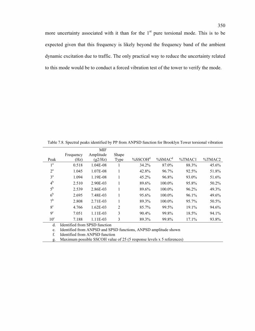
350

more uncertainty associated with it than for the 1st pure torsional mode. This is to be

expected given that this frequency is likely beyond the frequency band of the ambient

dynamic excitation due to traffic. The only practical way to reduce the uncertainty related

to this mode would be to conduct a forced vibration test of the tower to verify the mode.

Table 7.8. Spectral peaks identified by PP from ANPSD function for Brooklyn Tower torsional vibration

Peak Frequency

(Hz)

MIF Amplitude

(g2/Hz) Shape Type %SSCOHd %SMACd %TMAC1 %TMAC2

1a 0.518 1.04E-08 1 34.2% 87.0% 88.3% 45.6% 2a 1.045 1.07E-08 1 42.8% 96.7% 92.5% 51.8% 3a 1.094 1.19E-08 1 45.2% 96.8% 93.0% 51.6% 4b 2.510 2.90E-03 1 89.6% 100.0% 95.8% 50.2% 5b 2.539 2.86E-03 1 89.6% 100.0% 96.2% 49.3% 6b 2.695 7.48E-03 1 95.6% 100.0% 96.1% 49.6% 7b 2.808 2.71E-03 1 89.3% 100.0% 95.7% 50.5% 8c 4.766 1.62E-03 2 85.7% 99.5% 19.1% 94.6% 9c 7.051 1.11E-03 3 90.4% 99.8% 18.5% 94.1%

10c 7.188 1.11E-03 3 89.3% 99.8% 17.1% 93.8% d. Identified from SPSD function e. Identified from ANPSD and SPSD functions, ANPSD amplitude shown f. Identified from ANPSD function g. Maximum possible SSCOH value of 25 (5 response levels x 5 references)

351

Table 7.9. Comparison of %SSCOH values - tower torsional references and all other bridge responses

Peak (Hz)

MT Longa

MT Tora

MT Lata

BT Longb

BT Torb

BT Latc

MS Vertd

MS Tord

MS Latd

SS Vertd

SS Tord

SS Latd

0.518 1% 1% 1% 6% 34% 5% 2% 7% 0% 2% 26% 41% 1.045 1% 5% 2% 6% 43% 11% 5% 42% 32% 2% 23% 23% 1.094 2% 2% 1% 9% 45% 11% 4% 8% 1% 16% 49% 47% 2.510 6% 63% 26% 10% 90% 60% 2% 18% 51% 1% 34% 20% 2.539 7% 48% 23% 6% 90% 59% 1% 1% 38% 2% 26% 13% 2.695 1% 13% 5% 17% 96% 77% 0% 11% 4% 1% 12% 4% 2.808 3% 45% 7% 5% 89% 62% 3% 17% 19% 3% 1% 34% 4.766 13% 9% 11% 82% 86% 82% 1% 10% 14% 3% 18% 47% 7.051 1% 1% 1% 9% 90% 27% 3% 2% 11% 3% 7% 19% 7.188 2% 1% 3% 13% 89% 28% 2% 14% 24% 3% 20% 9% a. Maximum possible SSCOH value = (1.0 x r x l) = 1.0 x 5 x 1 = 5 b. Maximum possible SSCOH value = (1.0 x r x l) = 1.0 x 5 x 5 = 25 c. Maximum possible SSCOH value = (1.0 x r x l) = 1.0 x 5 x 10 = 50 d. Maximum possible SSCOH value = (1.0 x r x l) = 1.0 x 5 x 2 = 10

Table 7.10. Comparison of tower torsional spectral peaks with span identification results

Previous Span Test Current Span Measurements Spectral Peak

Frequency (Hz) Frequency

(Hz) Mode Description Frequency (Hz) Description

1 0.518 0.525 TS1 0.518 TS 2 1.045 1.056 TM5 1.045 TM 3 1.094 1.100 TS3, LS5 1.099 TS, LS 4 2.510 - - - - 5 2.539 - - 2.539 VM, TM, LM* - - 2.544 VS - - 2.676 VM

6 2.695 - - 2.695 TM 7 2.808 - - 2.808 VS 8 4.766 - - 4.766 LS* 9 7.051 - - 7.051 VM*, TM*

10 7.188 - - 7.188 TM VM = Main Span Vertical, TM = Main Span Torsional, LM = Main Span Lateral, VS = Side Span Vertical, TS = Side Span Torsional, LS = Side Span Lateral. *MIF magnitude at this frequency is at least an order of magnitude smaller than corresponding MIF value at frequencies that were characterized modes in previous span test

352

2.510 Hz (ANPSD & SPSD)

0

50

100

150

200

250

-1.0 -0.5 0.0 0.5 1.0

Blong

Clong

Elong

Glong

Hlong

0.518 Hz (SPSD)

0

50

100

150

200

250

-1.0 -0.5 0.0 0.5 1.0

Blong

Clong

Elong

Glong

Hlong

1.045 Hz (SPSD)

0

50

100

150

200

250

-1.0 -0.5 0.0 0.5 1.0

Blong

Clong

Elong

Glong

Hlong

1.094 Hz (SPSD)

0

50

100

150

200

250

-1.0 -0.5 0.0 0.5 1.0

Blong

Clong

Elong

Glong

Hlong


0

50

100

150

200

250

-1.0 -0.5 0.0 0.5 1.0

Blong

Clong

Elong

Glong

Hlong


0

50

100

150

200

250

-1.0 -0.5 0.0 0.5 1.0

Blong

Clong

Elong

Glong

Hlong

Hei

ght A

bove

Bas

e (f

t)


Hei

ght A

bove

Bas

e (f

t)

1 1 1 1

11


0

50

100

150

200

250

-1.0 -0.5 0.0 0.5 1.0

Blong

Clong

Elong

Glong

Hlong

1

4.766 Hz (ANPSD)

0

50

100

150

200

250

-1.0 -0.5 0.0 0.5 1.0

Blong

Clong

Elong

Glong

Hlong

2

7.051 Hz (ANPSD)

0

50

100

150

200

250

-1.0 -0.5 0.0 0.5 1.0

Blong

Clong

Elong

Glong

Hlong

7.188 Hz (ANPSD)

0

50

100

150

200

250

-1.0 -0.5 0.0 0.5 1.0

Blong

Clong

Elong

Glong

Hlong

Hei

ght A

bove

Bas

e (f

t)

3 3

Figure 7.14. Unit normalized operating deflection shapes for torsional spectral peaks

353

0.518 Level B Level C Level E Level G Level HLevel B 0.0 -106.2 -33.8 -7.8 -1.3Level C 106.2 0.0 1.1 -5.8 -15.4Level E 33.8 -1.1 0.0 -8.2 -3.8Level G 7.8 5.8 8.2 0.0 0.2Level H 1.3 15.4 3.8 -0.2 0.0



2.510 Level B Level C Level E Level G Level HLevel B 0.0 -0.5 2.7 0.1 1.0Level C 0.5 0.0 4.3 1.3 1.8Level E -2.7 -4.3 0.0 -2.9 -2.3Level G -0.1 -1.3 2.9 0.0 0.5Level H -1.0 -1.8 2.3 -0.5 0.0

2.539 Level B Level C Level E Level G Level HLevel B 0.0 -2.5 2.3 1.0 2.3Level C 2.5 0.0 4.5 3.4 5.0Level E -2.3 -4.5 0.0 -1.5 0.2Level G -1.0 -3.4 1.5 0.0 1.7Level H -2.3 -5.0 -0.2 -1.7 0.0

2

4.766 Level B Level C Level E Level G Level HLevel B 0.0 9.5 6.8 -176.8 -177.4Level C -9.5 0.0 -2.6 173.4 173.0Level E -6.8 2.6 0.0 176.2 175.9Level G 176.8 -173.4 -176.2 0.0 -0.2Level H 177.4 -173.0 -175.9 0.2 0.0

7.051 Level B Level C Level E Level G Level HLevel B 0.0 13.7 21.9 178.3 -166.7Level C -13.7 0.0 8.1 164.3 179.3Level E -21.9 -8.1 0.0 156.2 171.5Level G -178.3 -164.3 -156.2 0.0 14.9Level H 166.7 -179.3 -171.5 -14.9 0.0

7.188 Level B Level C Level E Level G Level HLevel B 0.0 13.0 20.8 179.8 -164.0Level C -13.0 0.0 7.9 167.5 -176.5Level E -20.8 -7.9 0.0 159.0 175.6Level G -179.8 -167.5 -159.0 0.0 14.3Level H 164.0 176.5 -175.6 -14.3 0.0

3

3

1

2.808 Level B Level C Level E Level G Level HLevel B 0.0 1.8 5.0 2.8 4.4Level C -1.8 0.0 2.9 1.1 1.8Level E -5.0 -2.9 0.0 -2.1 -1.2Level G -2.8 -1.1 2.1 0.0 0.9Level H -4.4 -1.8 1.2 -0.9 0.0

1

1

1

3

3


1

0.518 Level B Level C Level E Level G Level HLevel B 0.0 -106.2 -33.8 -7.8 -1.3Level C 106.2 0.0 1.1 -5.8 -15.4Level E 33.8 -1.1 0.0 -8.2 -3.8Level G 7.8 5.8 8.2 0.0 0.2Level H 1.3 15.4 3.8 -0.2 0.0




2.539 Level B Level C Level E Level G Level HLevel B 0.0 -2.5 2.3 1.0 2.3Level C 2.5 0.0 4.5 3.4 5.0Level E -2.3 -4.5 0.0 -1.5 0.2Level G -1.0 -3.4 1.5 0.0 1.7Level H -2.3 -5.0 -0.2 -1.7 0.0

22




3

3

1




33

33

11


1


11

11

11

33

33


11

Figure 7.15. Raw phase factors between each output-reference pair at torsional spectral peak frequencies

354

Table 7.11. Summary evaluation results for identifying pure torsional tower modes

Peak Freq. (Hz)

Shape Type

Max. MIF

Shape Plausibility

Shapes Agreea

Max %SSCOH

Tower %SMAC

>99% %TMACb %SSCOH

Bridgec Phase

Factord Span

Modes

1 0.518 1 T1 3

2 1.045 1 T1 2

3 1.094 1 T1 3

4 2.510 1 T1 1

5 2.539 1 T1 1

6 2.695 1 T1 1

7 2.808 1 T1 1

8 4.766 2 T2 1

9 7.051 3 T2 3

10 7.188 3 T2 3

a. Operating deflection shapes are visually consistent b. Correlation with analytical tower mode shapes c. Most coherent with only tower response for direction considered d. 1 = within +/- 10 degrees of zero or 180 degrees (most normal characteristics); 2 = +/- 20 degrees of zero or 180 degrees; 3 = greater than +/- 20 degrees of

zero or 180 degrees

355

7.4.3.3 SSI Method

The natural frequencies and mode shapes identified for the pure torsional response of

the Brooklyn Tower by the SSI method are shown in Figure 7.16 and Figure 7.17. A total

of 14 natural frequencies and mode shapes were identified in the torsional response

direction. There were four modes identified with frequencies that corresponded to the

locations of spectral peaks identified by the peak picking method (0.519 Hz, 1.096 Hz,

2.697 Hz, and 4.766 Hz). All but one of these frequencies (2.697 Hz) was excluded as

possible pure torsional modes of the Brooklyn Tower.

Several of the mode shapes corresponding to frequencies identified by the SSI

method are clearly implausible, and could be ruled out from the results. Other results are

more difficult to exclude without considering other parameters in conjunction with the

SSI results. Furthermore, if the dynamic characteristics of the tower had not been studied

beforehand, many of the modes identified by the SSI method could easily be considered

as valid results when it is clear from the other methods that they should not be considered

as pure torsional modes of the tower.

It should be noted that more modes were identified by the SSI method in this

response direction than was observed in the longitudinal response direction. The signal-

to-noise ratios of the measurements in the torsional response direction were generally

lower than in the longitudinal response direction. This is clearly an indication that this

method yields more reliable results when the signal-to-noise ratio of the measurements is

greater. It is also interesting that there was not as significant a difference in the

effectiveness of the peak picking method that was implemented for this study between

356

the longitudinal and torsional response directions. In fact, there were actually less peaks

identified by the peak picking implementation as only the most reliable spectral peaks

(those associated with the greatest signal-to-noise ratios) were retained for subsequent

analysis.

357

0.294 Hz

0

50

100

150

200

250

-1.0 -0.5 0.0 0.5 1.0

0.294

0.390 Hz

0

50

100

150

200

250

-1.0 -0.5 0.0 0.5 1.0

0.390

0.519 Hz

0

50

100

150

200

250

-1.0 -0.5 0.0 0.5 1.0

0.519

Hei

ght A

bove

Bas

e (f

t)


0

50

100

150

200

250

-1.0 -0.5 0.0 0.5 1.0

0.844

0.892 Hz

0

50

100

150

200

250

-1.0 -0.5 0.0 0.5 1.0

0.892

1.096 Hz

0

50

100

150

200

250

-1.0 -0.5 0.0 0.5 1.0

1.096

Hei

ght A

bove

Bas

e (f

t)

1.328 Hz

0

50

100

150

200

250

-1.0 -0.5 0.0 0.5 1.0

1.328

1.533 Hz

0

50

100

150

200

250

-1.0 -0.5 0.0 0.5 1.0

1.533Hei

ght A

bove

Bas

e (f

t)

2.697 Hz

0

50

100

150

200

250

-1.0 -0.5 0.0 0.5 1.0

2.697

Figure 7.16. Tower torsional modes by SSI method

358

2.726 Hz

0

50

100

150

200

250

-1.0 -0.5 0.0 0.5 1.0

2.726

3.640 Hz

0

50

100

150

200

250

-1.0 -0.5 0.0 0.5 1.0

3.640

4.766 Hz

0

50

100

150

200

250

-1.0 -0.5 0.0 0.5 1.0

4.766Hei

ght A

bove

Bas

e (f

t)


0

50

100

150

200

250

-1.0 -0.5 0.0 0.5 1.0

4.829

5.087 Hz

0

50

100

150

200

250

-1.0 -0.5 0.0 0.5 1.0

5.087Hei

ght A

bove

Bas

e (f

t)

Figure 7.17. Tower torsional modes by SSI method

7.4.3.4 PTD Method

The PTD method was applied to the experimental data from the torsional response



frequencies and mode shapes that were identified using the pIRF-corr approach and the

359

PTD method are shown in Figure 7.18. A total of 5 natural frequencies and mode shapes

were identified from the pure torsional vibration responses of the Brooklyn Tower. Three

of the natural frequencies identified by this approach (2.709 Hz, 4.766 Hz, and 7.143 Hz)

did correspond to spectral peaks that were identified by the peak picking method;

however, the mode shape associated with the frequency at 2.709 Hz is not very consistent

with the operating deflection shape identified by the peak picking method. The mode

shape at 7.143 Hz is more consistent with the operating deflection shape identified by the

peak picking method as the most likely 2nd pure torsional mode of the Brooklyn Tower.

The frequencies and mode shapes that were identified using the pIRF-RD approach

and the PTD method are shown in Figure 7.19. There were also 5 natural frequencies and

mode shapes identified from the pure torsional vibration responses of the Brooklyn

Tower using this approach. In this case, there were also three natural frequencies

identified (2.706 Hz, 4.767 Hz, and 7.143 Hz) that corresponded to spectral peaks

identified by the peak picking method for the same measurement data. The mode shapes

associated with the 2.706 Hz and 7.143 Hz are also reasonably consistent with the

operating deflection shapes associated with 2.695 Hz and 7.051 Hz, which were

identified as the likely first two pure torsional modes of the tower from the peak picking

method.

Of the two approaches used with the PTD method, the results from the pIRF-RD

approach were slightly more consistent with the results obtained from the peak picking

method. The results of the peak picking method were necessary for interpreting the

results from both PTD implementations as both approaches identified spurious results as

modes. The PTD method did identify fewer modes than the number identified by the SSI

360

method, but the identified modes still required additional interpretation to obtain results

that were consistent with those obtained from the peak picking method.

2.709 Hz

0

50

100

150

200

250

-1.0 -0.5 0.0 0.5 1.0

2.709

2.530 Hz

0

50

100

150

200

250

-1.0 -0.5 0.0 0.5 1.0

2.530

4.766 Hz

0

50

100

150

200

250

-1.0 -0.5 0.0 0.5 1.0

4.766

7.194 Hz

0

50

100

150

200

250

-1.0 -0.5 0.0 0.5 1.0

7.194

7.143 Hz

0

50

100

150

200

250

-1.0 -0.5 0.0 0.5 1.0

7.143

Hei

ght A

bove

Bas

e (f

t)


Hei

ght A

bove

Bas

e (f

t)

Figure 7.18. Brooklyn Tower torsional modes by PTD from correlation functions

361

2.492 Hz

0

50

100

150

200

250

-1.0 -0.5 0.0 0.5 1.0

2.492

3.828 Hz

0

50

100

150

200

250

-1.0 -0.5 0.0 0.5 1.0

3.828

2.706 Hz

0

50

100

150

200

250

-1.0 -0.5 0.0 0.5 1.0

2.706

4.767 Hz

0

50

100

150

200

250

-1.0 -0.5 0.0 0.5 1.0

4.767

7.143 Hz

0

50

100

150

200

250

-1.0 -0.5 0.0 0.5 1.0

5.245

Hei

ght A

bove

Bas

e (f

t)


Hei

ght A

bove

Bas

e (f

t)

Figure 7.19. Brooklyn Tower torsional modes by PTD from random decrement functions

7.4.3.5 CMIF Method

The CMIF method was applied to the experimental data from the torsional response



frequencies and mode shapes that were identified using the pIRF-corr approach and the

362

CMIF method are shown in Figure 7.20 and Figure 7.21. A total of 14 natural frequencies

and mode shapes were identified from the pure torsional vibration responses of the

Brooklyn Tower. Only two of the natural frequencies identified using this approach

(2.721 Hz and 4.837 Hz) were relatively close to the frequencies of spectral peaks

identified by the peak picking method. The mode shapes associated with these natural

frequencies were not consistent with the corresponding operating deflection shapes for

the frequencies identified as the most likely pure torsional tower modes by the peak

picking method. The CMIF method did identify a mode at 2.422 Hz, and the mode shape

associated with this frequency is consistent with the shape expected for the 1st pure

torsional tower mode; however, this frequency is 10% less than the corresponding

frequency of the 1st pure torsional mode that was identified by the other identification

methods. Most of the remaining natural frequencies identified by this method are likely

spurious results when they are considered in the context of the peak picking results. The

spurious results may be interpreted as real modes of the structure if these results are not

considered within the context of the other identification results or the output from a finite

element model of the bridge.

The natural frequencies and mode shapes identified by the CMIF method applied to

pseudo impulse response functions that were estimated from Random Decrement

functions for the pure torsional vibration responses of the Brooklyn Tower are shown in

Figure 7.22 and Figure 7.23. A total of 18 natural frequencies and mode shapes were

identified by this approach from the pure torsional vibration responses of the Brooklyn

Tower. Many of the mode shapes computed by this method are very similar for multiple

frequencies. There were 4 natural frequencies that were somewhat consistent with

363

spectral peaks identified from the peak picking method (2.726 Hz, 4.733 Hz, 6.995 Hz,

and 7.235 Hz). The mode shape associated with 2.726 Hz is consistent with the operating

deflection shapes at the most likely 1st pure torsional mode identified from peak picking

(2.695 Hz). The mode shape at 6.995 Hz is also relatively consistent with the operating

deflection shapes at the most likely 2nd pure torsional mode identified from peak picking

(7.051 Hz).

The number of natural frequencies identified by the CMIF method using two different

approaches was comparable to the number obtained from the SSI method. There were

more natural frequencies identified by this method than both the peak picking and PTD

methods. The natural frequencies and mode shapes found using the pIRF-RD approach

for the CMIF method were slightly more consistent with the peak picking results at the

two frequencies identified as the most likely pure torsional tower modes than those from

the pIRF-corr approach. As was the case with the other more advanced identification

methods applied to the torsional vibration response of the Brooklyn Tower, the complete

set of identified natural frequencies and mode shapes still contained many spurious

results that could only be identified and ruled out by considering the results from the peak

picking method or by using the results from a finite element model.

364

2.422 Hz

0

50

100

150

200

250

-1.0 -0.5 0.0 0.5 1.0

2.422

2.721 Hz

0

50

100

150

200

250

-1.0 -0.5 0.0 0.5 1.0

2.721

4.837 Hz

0

50

100

150

200

250

-1.0 -0.5 0.0 0.5 1.0

4.837

5.956 Hz

0

50

100

150

200

250

-1.0 -0.5 0.0 0.5 1.0

5.956

7.686 Hz

0

50

100

150

200

250

-1.0 -0.5 0.0 0.5 1.0

7.686

7.666 Hz

0

50

100

150

200

250

-1.0 -0.5 0.0 0.5 1.0

7.666

7.902 Hz

0

50

100

150

200

250

-1.0 -0.5 0.0 0.5 1.0

7.902

7.765 Hz

0

50

100

150

200

250

-1.0 -0.5 0.0 0.5 1.0

7.765

Hei

ght A

bove

Bas

e (f

t)


Figure 7.20. Brooklyn Tower torsional modes by CMIF from correlation functions

365

8.408 Hz

0

50

100

150

200

250

-1.0 -0.5 0.0 0.5 1.0

8.408

8.377 Hz

0

50

100

150

200

250

-1.0 -0.5 0.0 0.5 1.0

8.377

8.574 Hz

0

50

100

150

200

250

-1.0 -0.5 0.0 0.5 1.0

8.574

9.090 Hz

0

50

100

150

200

250

-1.0 -0.5 0.0 0.5 1.0

9.090

8.840 Hz

0

50

100

150

200

250

-1.0 -0.5 0.0 0.5 1.0

8.840

8.634 Hz

0

50

100

150

200

250

-1.0 -0.5 0.0 0.5 1.0

8.634

Hei

ght A

bove

Bas

e (f

t)


Figure 7.21. Brooklyn Tower torsional modes by CMIF from correlation functions

366

2.427 Hz

0

50

100

150

200

250

-1.0 -0.5 0.0 0.5 1.0

2.427

Hei

ght A

bove

Bas

e (f

t)


2.744 Hz

0

50

100

150

200

250

-1.0 -0.5 0.0 0.5 1.0

2.744

2.726 Hz

0

50

100

150

200

250

-1.0 -0.5 0.0 0.5 1.0

2.726

4.733 Hz

0

50

100

150

200

250

-1.0 -0.5 0.0 0.5 1.0

4.733

5.431 Hz

0

50

100

150

200

250

-1.0 -0.5 0.0 0.5 1.0

5.431

5.505 Hz

0

50

100

150

200

250

-1.0 -0.5 0.0 0.5 1.0

5.505

Hei

ght A

bove

Bas

e (f

t)

5.581 Hz

0

50

100

150

200

250

-1.0 -0.5 0.0 0.5 1.0

5.581

Hei

ght A

bove

Bas

e (f

t)

6.995 Hz

0

50

100

150

200

250

-1.0 -0.5 0.0 0.5 1.0

6.995

6.956 Hz

0

50

100

150

200

250

-1.0 -0.5 0.0 0.5 1.0

6.956

Figure 7.22. Brooklyn Tower torsional modes by CMIF from random decrement functions

367

7.235 Hz

0

50

100

150

200

250

-1.0 -0.5 0.0 0.5 1.0

7.235

Hei

ght A

bove

Bas

e (f

t)


7.255 Hz

0

50

100

150

200

250

-1.0 -0.5 0.0 0.5 1.0

7.255

7.815 Hz

0

50

100

150

200

250

-1.0 -0.5 0.0 0.5 1.0

7.815

7.916 Hz

0

50

100

150

200

250

-1.0 -0.5 0.0 0.5 1.0

7.916

Hei

ght A

bove

Bas

e (f

t)

8.560 Hz

0

50

100

150

200

250

-1.0 -0.5 0.0 0.5 1.0

8.560

8.599 Hz

0

50

100

150

200

250

-1.0 -0.5 0.0 0.5 1.0

8.599

8.860 Hz

0

50

100

150

200

250

-1.0 -0.5 0.0 0.5 1.0

8.860

Hei

ght A

bove

Bas

e (f

t)

9.261 Hz

0

50

100

150

200

250

-1.0 -0.5 0.0 0.5 1.0

9.261

9.373 Hz

0

50

100

150

200

250

-1.0 -0.5 0.0 0.5 1.0

9.373

Figure 7.23. Brooklyn Tower torsional modes by CMIF from random decrement functions

368

7.4.4 Tower Lateral Natural Frequencies and Mode Shapes

7.4.4.1 Lateral Spectral Peaks Identified by PP

The spectral peaks identified by the peak picking method for the lateral vibration

response of the Brooklyn Tower are summarized in Table 7.12. The spectral peaks shown

in the table were identified from the ANPSD function. The spectral peaks that were also

identified by the other MIFs used in this study are also noted in the table. The amplitude

of the MIF, the %SSCOH, %SMAC and %TMAC values associated with each spectral

peak are also summarized in the table. The %TMAC parameter was computed using the

first two lateral mode shapes from the idealized analytical model that was discussed in

Chapter 5. The %SMAC and %TMAC results shown in Table 7.12 were computed using

the operating deflection shapes estimated for the north column of the Brooklyn Tower.

The unit normalized operating deflection shapes associated with each spectral peak

were computed using the lateral response at each measurement level on the Brooklyn

Tower as a reference level. These shapes were computed independently for the north,

middle and south columns (above the roadway level) of the Brooklyn Tower. The

measurement data used to compute these shapes was the same in each case for the lower

levels on the tower (Levels B, C and E). The unit normalized operating deflection shapes

computed at the identified spectral peak frequencies for the north tower column are

shown in Figure 7.24 and Figure 7.25. The unit normalized operating deflection shapes

computed at the identified spectral peak frequencies for the middle tower column are

shown in Figure 7.26 and Figure 7.27. Finally, the unit normalized operating deflection

shapes computed at the identified spectral peak frequencies for the south tower column

are shown in Figure 7.28 and Figure 7.29. The operating deflection shapes are shown for

369

all three columns to verify their consistency with each other in the same response

direction. The analysis of the idealized analytical model also indicated that the lateral

response of each tower column should be relatively consistent for the lateral tower

modes.

The operating deflection shapes computed for each column of the Brooklyn Tower

were classified according to 4 different types of shapes. The resulting shape type

classification for each identified spectral peak is summarized in Table 7.12. The shape

type classifications were the same for the north, middle and south tower columns.

The %SSCOH values computed between the Brooklyn Tower lateral vibration

response and all other bridge vibration responses for the frequencies associated with the

identified lateral peaks are summarized in Table 7.13. The %SSCOH parameter was

calculated using all 10 lateral accelerometers on the Brooklyn Tower (one sensor at

Levels B, C, E, H and three sensors at Levels F and G) as references. The %SSCOH

values computed using only the Brooklyn Tower lateral accelerometers (BT Lat) are the

same values that were reported for the %SSCOH values in Table 7.12.

The frequencies corresponding to the identified spectral peaks for the lateral vibration

response of the Brooklyn Tower are compared with the natural frequencies of the spans

from an earlier experimental characterization of the spans conducted by others using

ambient and forced vibration testing, and with the spectral peaks identified for the spans

from the current study in Table 7.14. The MIF used in the current study for identifying

spectral peaks associated with span responses was the SPSD function.

The raw phase factors (angles) associated with each identified spectral peak are

reported for each lateral tower response reference location in Figure 7.30 and Figure 7.31.

370

These values were whitewashed to force normal mode characteristics on the operating

deflection shapes computed for each spectral peak. The circled numbers next the phase

factors for each spectral peak frequency shown in the figures indicate the level to which

the values corresponded to normal mode characteristics.

7.4.4.2 Identification of Lateral Modes from Identified Spectral Peaks

There were a total of 12 spectral peaks identified from the lateral vibration response

measurements by the peak picking method implemented in this study. As was the case

with the other primary response directions, the analysis of the idealized analytical model

of the Brooklyn Bridge indicated that there should be two pure lateral tower modes for

the frequency range of the identification results. The 12 spectral peaks identified for this

response direction from the experimental data should therefore only be considered as

possible candidates for the pure lateral tower modes. The identified spectral peaks for the

lateral response direction were evaluated using the same procedure employed for the pure

longitudinal and torsional response directions. The results of the evaluation process for

the characteristics and parameters associated with each identified spectral peak are


Many of the identified spectral peaks may be ruled out for consideration as being pure

lateral modes of the tower based on the results of this evaluation shown in Table 7.15.

The operating deflection shapes associated with the last three spectral peaks are

inconsistent. In addition, these frequencies rate very poorly as possible candidates for the

lateral tower modes based on the results the remaining evaluation criteria. The spectral

peak at 2.695 Hz could be considered as a possible candidate for a lateral mode, but this

371

frequency generally does not rate very highly based on the results of the evaluation

criteria. This frequency was also identified by the peak picking method as the most likely

candidate for the 1st torsional mode of the Brooklyn Tower. In Chapter 4, it was shown

that the spectral peak in the lateral response direction at 2.695 Hz was the result of the

lateral accelerometers being installed on the face of the tower. The lateral accelerometers

were eccentric to the center of rotation of the tower (except at the top of the tower) and

their response will also peak at the torsional modes of the tower.

When the results of the individual evaluation criteria are considered together for the

remaining spectral peaks, it is clear that the most likely candidate for the 1st pure lateral

mode of the Brooklyn Tower is the spectral peak at 1.597 Hz. The most likely candidate

for the 2nd pure lateral mode of the Brooklyn Tower is less clear cut based on the results

of the different evaluation criteria. The spectral peaks identified at 4.668 Hz and 4.766

Hz are both good candidates for the 2nd lateral mode. The amplitudes of the MIF

functions at both frequencies are very close to each other, although the MIF is slightly

larger at 4.766 Hz. The results of the other evaluation criteria tend to indicate the most

likely 2nd lateral mode is the spectral peak at 4.668 Hz, but the differences between these

parameters for the two frequencies are very slight. The %SSCOH parameter values listed

in Table 7.13 indicate that there is some interaction between the other response directions

of the Brooklyn Tower with its lateral response at both frequencies (longitudinal at 4.668

Hz, and both longitudinal and torsion at 4.766 Hz). Furthermore, the %SSCOH values

also indicate that the side span has some lateral interaction with the Brooklyn Tower at

4.766 Hz; however, there were no span modes identified at either of these frequencies

372

from the previous experimental characterization of the spans. This could indicate that the

lateral response of the tower is driving the lateral response of the side span at 4.766 Hz.

The factors described above lead to some uncertainty being associated with the

selection of one of these two frequencies as the more likely 2nd lateral mode of the tower

that is in addition to the uncertainty already associated with both spectral peaks based on

the evaluation criteria (operating deflection shapes not exactly the same for all references,

etc.). Selecting one of these frequencies as the most likely mode will depend on the

relative importance assigned to each of the parameters considered in the evaluation

process. In this case, the amplitude of the MIF should be given a higher priority as an

indicator of the most likely mode because the MIF amplitude value directly relates to the

amplitude of the structural response. As a result, the spectral peak at 4.766 Hz is selected

as the more likely 2nd lateral mode of the Brooklyn Tower. It should be noted that the

location of this mode can really only be verified by a forced excitation test, and given the

uncertainty associated with its identification, this frequency should be considered as a

possible guide for designing such a test.

373

Table 7.12. Spectral peaks identified by PP from ANPSD function for Brooklyn Tower lateral vibrations

Peak Frequency

(Hz)

MIF Amplitude

(g2/Hz)

Shape Type %SSCOHa %SMACa %TMAC1 %TMAC2

1 1.426 1.24E-03 1 61.39% 93.1% 91.0% 3.1% 2b,c 1.597 1.14E-02 1 93.68% 99.8% 98.1% 5.1% 3c 1.699c 1.57E-03 1 73.90% 98.1% 97.0% 5.4% 4 2.695 1.26E-03 2 66.23% 91.4% 58.0% 1.9%

5b,c 4.468 1.40E-03 3 58.82% 98.2% 12.3% 91.3% 6 4.536 2.58E-03 3 70.00% 99.5% 12.6% 91.7%

7b,c 4.668 2.33E-02 3 92.78% 100.0% 11.2% 92.5% 8b,c 4.766 2.37E-02 3 92.20% 100.0% 11.3% 93.1% 9 5.000 3.28E-03 3 63.23% 80.9% 12.2% 83.9%

10 9.233 1.22E-03 4 36.97% 89.7% 34.6% 8.4% 11 9.263 1.18E-03 4 37.13% 88.4% 32.4% 9.1% 12 9.302 1.17E-03 4 36.49% 71.4% 29.2% 11.8%

a. Maximum possible SSCOH value of 100 (10 responses x 10 references) b. Spectral peak at this frequency also identified in SPSD MIF c. Spectral peak at this frequency also identified in SSCSD MIF

Table 7.13. Comparison of %SSCOH values - tower lateral references and all other bridge responses

Peak (Hz)

MT Longa

MT Tora

MT Lata

BT Longb

BT Torb

BT Latc

MS Vertd

MS Tord

MS Latd

SS Vertd

SS Tord

SS Latd

1.426 10% 13% 30% 13% 23% 61% 2% 5% 54% 4% 13% 13% 1.597 0% 1% 1% 4% 10% 94% 1% 19% 20% 15% 50% 72% 1.699 1% 0% 1% 6% 15% 74% 4% 20% 22% 7% 13% 37% 2.695 1% 10% 4% 13% 77% 66% 0% 11% 4% 0% 9% 3% 4.468 1% 1% 2% 47% 13% 59% 1% 3% 6% 3% 1% 4% 4.536 1% 5% 0% 47% 17% 70% 0% 3% 6% 2% 0% 4% 4.668 12% 2% 17% 86% 53% 93% 3% 5% 11% 6% 5% 18% 4.766 15% 7% 11% 89% 82% 92% 1% 10% 16% 3% 15% 46% 5.000 3% 7% 8% 47% 31% 63% 1% 2% 3% 2% 2% 27% 9.233 3% 12% 22% 15% 15% 37% 5% 2% 5% 2% 4% 2% 9.263 7% 13% 23% 12% 16% 37% 4% 2% 4% 3% 3% 2% 9.302 6% 5% 16% 10% 15% 36% 3% 3% 3% 4% 4% 2% a. Maximum possible SSCOH value = (1.0 x r x l) = 1.0 x 10 x 1 = 10 b. Maximum possible SSCOH value = (1.0 x r x l) = 1.0 x 10 x 5 = 50 c. Maximum possible SSCOH value = (1.0 x r x l) = 1.0 x 10 x 10 = 100 d. Maximum possible SSCOH value = (1.0 x r x l) = 1.0 x 10 x 2 = 20

374

Table 7.14. Comparison of tower lateral spectral peaks with span identification results

Previous Span Test Current Span Measurements Spectral Peak

Frequency (Hz) Frequency (Hz) Mode Description Frequency (Hz) Description

1 1.426 - - 1.426 LM 2 1.597 - - - - 3 1.699 - - - - 2.676 VM

4 2.695 - - 2.695 TM* 5 4.468 - - - - 6 4.536 - - - - 7 4.668 - - - - 8 4.766 - - 4.766 LS* 9 5.000 - - 5.000 LS*

10 9.233 - - 9.238 LM* 11 9.263 - - - - 12 9.302 - - - -

VM = Main Span Vertical, TM = Main Span Torsional, LM = Main Span Lateral, VS = Side Span Vertical, TS = Side Span Torsional, LS = Side Span Lateral. *MIF magnitude at this frequency is at least an order of magnitude smaller than corresponding MIF value at frequencies that were characterized modes in previous span test

375

Hei

ght A

bove

Bas

e (f

t)


1.426 Hz

0

50

100

150

200

250

-1.5 -1.0 -0.5 0.0 0.5 1.0 1.5

B LAT

C LAT

E LAT

FN LAT

GN LAT

HLAT

1.597 Hz

0

50

100

150

200

250

-1.5 -1.0 -0.5 0.0 0.5 1.0 1.5

B LAT

C LAT

E LAT

FN LAT

GN LAT

HLAT

1.699 Hz

0

50

100

150

200

250

-1.5 -1.0 -0.5 0.0 0.5 1.0 1.5

B LAT

C LAT

E LAT

FN LAT

GN LAT

HLAT

2.695 Hz

0

50

100

150

200

250

-1.5 -1.0 -0.5 0.0 0.5 1.0 1.5

B LAT

C LAT

E LAT

FN LAT

GN LAT

HLAT

Hei

ght A

bove

Bas

e (f

t)

4.468 Hz

0

50

100

150

200

250

-1.5 -1.0 -0.5 0.0 0.5 1.0 1.5

B LAT

C LAT

E LAT

FN LAT

GN LAT

HLAT

4.536 Hz

0

50

100

150

200

250

-1.5 -1.0 -0.5 0.0 0.5 1.0 1.5

B LAT

C LAT

E LAT

FN LAT

GN LAT

HLAT

Figure 7.24. Unit normalized operating deflection shapes for lateral spectral peaks (north tower column)

376

4.668 Hz

0

50

100

150

200

250

-1.5 -1.0 -0.5 0.0 0.5 1.0 1.5

B LAT

C LAT

E LAT

FN LAT

GN LAT

HLAT

4.766 Hz

0

50

100

150

200

250

-1.5 -1.0 -0.5 0.0 0.5 1.0 1.5

B LAT

C LAT

E LAT

FN LAT

GN LAT

HLAT

5.000 Hz

0

50

100

150

200

250

-1.5 -1.0 -0.5 0.0 0.5 1.0 1.5

B LAT

C LAT

E LAT

FN LAT

GN LAT

HLAT

9.233 Hz

0

50

100

150

200

250

-1.5 -1.0 -0.5 0.0 0.5 1.0 1.5

B LAT

C LAT

E LAT

FN LAT

GN LAT

HLAT

Hei

ght A

bove

Bas

e (f

t)


Hei

ght A

bove

Bas

e (f

t)

9.263 Hz

0

50

100

150

200

250

-1.5 -1.0 -0.5 0.0 0.5 1.0 1.5

B LAT

C LAT

E LAT

FN LAT

GN LAT

HLAT

9.302 Hz

0

50

100

150

200

250

-1.5 -1.0 -0.5 0.0 0.5 1.0 1.5

B LAT

C LAT

E LAT

FN LAT

GN LAT

HLAT

Figure 7.25. Unit normalized operating deflection shapes for lateral spectral peaks (north tower column)

377

1.426 Hz

0

50

100

150

200

250

-1.5 -1.0 -0.5 0.0 0.5 1.0 1.5

B LAT

C LAT

E LAT

FN LAT

GN LAT

HLAT

1.597 Hz

0

50

100

150

200

250

-1.5 -1.0 -0.5 0.0 0.5 1.0 1.5

B LAT

C LAT

E LAT

FN LAT

GN LAT

HLAT

1.699 Hz

0

50

100

150

200

250

-1.5 -1.0 -0.5 0.0 0.5 1.0 1.5

B LAT

C LAT

E LAT

FN LAT

GN LAT

HLAT

2.695 Hz

0

50

100

150

200

250

-1.5 -1.0 -0.5 0.0 0.5 1.0 1.5

B LAT

C LAT

E LAT

FN LAT

GN LAT

HLAT

4.468 Hz

0

50

100

150

200

250

-1.5 -1.0 -0.5 0.0 0.5 1.0 1.5

B LAT

C LAT

E LAT

FN LAT

GN LAT

HLAT

4.536 Hz

0

50

100

150

200

250

-1.5 -1.0 -0.5 0.0 0.5 1.0 1.5

B LAT

C LAT

E LAT

FN LAT

GN LAT

HLAT

Hei

ght A

bove

Bas

e (f

t)


Hei

ght A

bove

Bas

e (f

t)

Figure 7.26. Unit normalized operating deflection shapes for lateral spectral peaks (middle tower column)

378

4.668 Hz

0

50

100

150

200

250

-1.5 -1.0 -0.5 0.0 0.5 1.0 1.5

B LAT

C LAT

E LAT

FN LAT

GN LAT

HLAT

4.766 Hz

0

50

100

150

200

250

-1.5 -1.0 -0.5 0.0 0.5 1.0 1.5

B LAT

C LAT

E LAT

FN LAT

GN LAT

HLAT

5.000 Hz

0

50

100

150

200

250

-1.5 -1.0 -0.5 0.0 0.5 1.0 1.5

B LAT

C LAT

E LAT

FN LAT

GN LAT

HLAT

9.233 Hz

0

50

100

150

200

250

-1.5 -1.0 -0.5 0.0 0.5 1.0 1.5

B LAT

C LAT

E LAT

FN LAT

GN LAT

HLAT

9.263 Hz

0

50

100

150

200

250

-1.5 -1.0 -0.5 0.0 0.5 1.0 1.5

B LAT

C LAT

E LAT

FN LAT

GN LAT

HLAT

9.302 Hz

0

50

100

150

200

250

-1.5 -1.0 -0.5 0.0 0.5 1.0 1.5

B LAT

C LAT

E LAT

FN LAT

GN LAT

HLAT

Hei

ght A

bove

Bas

e (f

t)


Hei

ght A

bove

Bas

e (f

t)

Figure 7.27. Unit normalized operating deflection shapes for lateral spectral peaks (middle tower column)

379

1.426 Hz

0

50

100

150

200

250

-1.5 -1.0 -0.5 0.0 0.5 1.0 1.5

B LAT

C LAT

E LAT

FN LAT

GN LAT

HLAT

1.597 Hz

0

50

100

150

200

250

-1.5 -1.0 -0.5 0.0 0.5 1.0 1.5

B LAT

C LAT

E LAT

FN LAT

GN LAT

HLAT

1.699 Hz

0

50

100

150

200

250

-1.5 -1.0 -0.5 0.0 0.5 1.0 1.5

B LAT

C LAT

E LAT

FN LAT

GN LAT

HLAT

2.695 Hz

0

50

100

150

200

250

-1.5 -1.0 -0.5 0.0 0.5 1.0 1.5

B LAT

C LAT

E LAT

FN LAT

GN LAT

HLAT


Hei

ght A

bove

Bas

e (f

t)H

eigh

t Abo

ve B

ase

(ft)

4.468 Hz

0

50

100

150

200

250

-1.5 -1.0 -0.5 0.0 0.5 1.0 1.5

B LAT

C LAT

E LAT

FN LAT

GN LAT

HLAT

4.536 Hz

0

50

100

150

200

250

-1.5 -1.0 -0.5 0.0 0.5 1.0 1.5

B LAT

C LAT

E LAT

FN LAT

GN LAT

HLAT

Figure 7.28. Unit normalized operating deflection shapes for lateral spectral peaks (south tower column)

380

4.668 Hz

0

50

100

150

200

250

-1.5 -1.0 -0.5 0.0 0.5 1.0 1.5

B LAT

C LAT

E LAT

FN LAT

GN LAT

HLAT

4.766 Hz

0

50

100

150

200

250

-1.5 -1.0 -0.5 0.0 0.5 1.0 1.5

B LAT

C LAT

E LAT

FN LAT

GN LAT

HLAT

5.000 Hz

0

50

100

150

200

250

-1.5 -1.0 -0.5 0.0 0.5 1.0 1.5

B LAT

C LAT

E LAT

FN LAT

GN LAT

HLAT

9.263 Hz

0

50

100

150

200

250

-1.5 -1.0 -0.5 0.0 0.5 1.0 1.5

B LAT

C LAT

E LAT

FN LAT

GN LAT

HLAT

9.302 Hz

0

50

100

150

200

250

-1.5 -1.0 -0.5 0.0 0.5 1.0 1.5

B LAT

C LAT

E LAT

FN LAT

GN LAT

HLAT

9.233 Hz

0

50

100

150

200

250

-1.5 -1.0 -0.5 0.0 0.5 1.0 1.5

B LAT

C LAT

E LAT

FN LAT

GN LAT

HLAT


Hei

ght A

bove

Bas

e (f

t)H

eigh

t Abo

ve B

ase

(ft)

Figure 7.29. Unit normalized operating deflection shapes for lateral spectral peaks (south tower column)

381

1.426 Level B Level C Level E Level FN Level FS Level FM Level GN Level GS Level GM Level HLevel B 0.0 21.6 9.3 11.2 -5.8 0.8 16.8 4.8 -0.9 1.4Level C -21.6 0.0 -3.0 -5.9 -17.7 -10.0 -1.9 -8.1 -11.9 -8.0Level E -9.3 3.0 0.0 -2.5 -13.9 -6.3 1.7 -4.2 -7.9 -5.4Level FN -11.2 5.9 2.5 0.0 -11.4 -4.8 4.7 -2.1 -6.0 -2.8Level FS 5.8 17.7 13.9 11.4 0.0 6.4 18.2 9.1 3.5 7.5Level FM -0.8 10.0 6.3 4.8 -6.4 0.0 7.1 2.7 -1.4 1.0Level GN -16.8 1.9 -1.7 -4.7 -18.2 -7.1 0.0 -5.4 -8.4 -8.4Level GS -4.8 8.1 4.2 2.1 -9.1 -2.7 5.4 0.0 -3.9 -0.8Level GM 0.9 11.9 7.9 6.0 -3.5 1.4 8.4 3.9 0.0 3.0Level H -1.4 8.0 5.4 2.8 -7.5 -1.0 8.4 0.8 -3.0 0.0

1.597 Level B Level C Level E Level FN Level FS Level FM Level GN Level GS Level GM Level HLevel B 0.0 3.1 1.8 -3.1 -4.3 -3.5 -2.5 -3.8 -4.4 -3.4Level C -3.1 0.0 -0.7 -5.6 -6.9 -6.5 -4.8 -6.4 -7.0 -6.1Level E -1.8 0.7 0.0 -4.9 -6.2 -5.5 -4.4 -5.7 -6.2 -5.3Level FN 3.1 5.6 4.9 0.0 -1.3 -0.7 0.6 -0.8 -1.2 -0.4Level FS 4.3 6.9 6.2 1.3 0.0 0.5 1.8 0.5 0.0 0.9Level FM 3.5 6.5 5.5 0.7 -0.5 0.0 1.3 -0.1 -0.5 0.3Level GN 2.5 4.8 4.4 -0.6 -1.8 -1.3 0.0 -1.3 -1.9 -1.0Level GS 3.8 6.4 5.7 0.8 -0.5 0.1 1.3 0.0 -0.4 0.4Level GM 4.4 7.0 6.2 1.2 0.0 0.5 1.9 0.4 0.0 0.9Level H 3.4 6.1 5.3 0.4 -0.9 -0.3 1.0 -0.4 -0.9 0.0

1.699 Level B Level C Level E Level FN Level FS Level FM Level GN Level GS Level GM Level HLevel B 0.0 -4.8 -1.3 -5.9 -5.0 -6.9 -6.3 -7.7 -6.9 -4.2Level C 4.8 0.0 0.4 -5.4 -2.1 -6.8 -3.8 -5.0 -4.3 -1.8Level E 1.3 -0.4 0.0 -6.1 -3.7 -7.0 -0.7 -6.6 -6.2 -2.7Level FN 5.9 5.4 6.1 0.0 2.1 -1.7 2.6 -0.6 -1.1 2.9Level FS 5.0 2.1 3.7 -2.1 0.0 -3.6 0.5 -3.2 -3.1 1.1Level FM 6.9 6.8 7.0 1.7 3.6 0.0 3.9 1.0 0.8 4.8Level GN 6.3 3.8 0.7 -2.6 -0.5 -3.9 0.0 -4.8 -2.7 0.6Level GS 7.7 5.0 6.6 0.6 3.2 -1.0 4.8 0.0 0.2 3.9Level GM 6.9 4.3 6.2 1.1 3.1 -0.8 2.7 -0.2 0.0 4.0Level H 4.2 1.8 2.7 -2.9 -1.1 -4.8 -0.6 -3.9 -4.0 0.0

2.695 Level B Level C Level E Level FN Level FS Level FM Level GN Level GS Level GM Level HLevel B 0.0 0.6 -1.3 -2.7 -3.9 -2.9 -0.8 -2.2 -1.4 -1.6Level C -0.6 0.0 0.1 -1.0 -1.9 -2.1 1.0 -0.6 0.0 0.7Level E 1.3 -0.1 0.0 -2.2 -2.7 -3.3 -0.3 -1.4 -1.1 -8.1Level FN 2.7 1.0 2.2 0.0 -1.0 -1.0 3.2 1.0 0.9 6.3Level FS 3.9 1.9 2.7 1.0 0.0 -0.2 2.8 1.6 2.0 0.6Level FM 2.9 2.1 3.3 1.0 0.2 0.0 2.4 1.5 1.9 1.7Level GN 0.8 -1.0 0.3 -3.2 -2.8 -2.4 0.0 -1.9 -1.4 4.4Level GS 2.2 0.6 1.4 -1.0 -1.6 -1.5 1.9 0.0 0.2 -3.8Level GM 1.4 0.0 1.1 -0.9 -2.0 -1.9 1.4 -0.2 0.0 1.6Level H 1.6 -0.7 8.1 -6.3 -0.6 -1.7 -4.4 3.8 -1.6 0.0

4.468 Level B Level C Level E Level FN Level FS Level FM Level GN Level GS Level GM Level HLevel B 0.0 2.3 2.1 -10.4 -5.0 178.5 -177.4 175.4 -179.2 175.9Level C -2.3 0.0 -0.3 -12.8 -8.2 175.8 -179.8 173.1 178.4 173.6Level E -2.1 0.3 0.0 -12.1 -7.1 178.1 -178.8 173.3 178.7 174.0Level FN 10.4 12.8 12.1 0.0 7.2 -166.5 -162.1 -174.8 -168.0 -174.8Level FS 5.0 8.2 7.1 -7.2 0.0 -164.9 -172.4 -179.8 -174.2 -179.2Level FM -178.5 -175.8 -178.1 166.5 164.9 0.0 -8.5 -2.9 1.9 -4.5Level GN 177.4 179.8 178.8 162.1 172.4 8.5 0.0 -5.4 -2.4 -7.4Level GS -175.4 -173.1 -173.3 174.8 179.8 2.9 5.4 0.0 5.4 0.4Level GM 179.2 -178.4 -178.7 168.0 174.2 -1.9 2.4 -5.4 0.0 -4.4Level H -175.9 -173.6 -174.0 174.8 179.2 4.5 7.4 -0.4 4.4 0.0

4.766 Level B Level C Level E Level FN Level FS Level FM Level GN Level GS Level GM Level HLevel B 0.0 -0.4 -0.7 -4.2 -3.6 167.9 178.0 176.7 177.5 176.9Level C 0.4 0.0 -0.3 -3.8 -3.2 168.2 178.4 177.1 177.9 177.4Level E 0.7 0.3 0.0 -3.6 -3.0 168.5 178.6 177.4 178.2 177.6Level FN 4.2 3.8 3.6 0.0 0.4 171.8 -177.7 -179.0 -178.2 -178.8Level FS 3.6 3.2 3.0 -0.4 0.0 171.9 -178.1 -179.6 -178.8 -179.4Level FM -167.9 -168.2 -168.5 -171.8 -171.9 0.0 10.4 8.6 9.5 9.1Level GN -178.0 -178.4 -178.6 177.7 178.1 -10.4 0.0 -1.2 -0.4 -1.0Level GS -176.7 -177.1 -177.4 179.0 179.6 -8.6 1.2 0.0 0.8 0.2Level GM -177.5 -177.9 -178.2 178.2 178.8 -9.5 0.4 -0.8 0.0 -0.6Level H -176.9 -177.4 -177.6 178.8 179.4 -9.1 1.0 -0.2 0.6 0.0

2

1

1

1

2

2

4.536 Level B Level C Level E Level FN Level FS Level FM Level GN Level GS Level GM Level HLevel B 0.0 2.0 1.7 -8.4 -5.5 -168.7 179.4 178.1 -179.0 178.4Level C -2.0 0.0 -0.3 -10.7 -7.7 -169.5 177.8 176.0 179.0 176.4Level E -1.7 0.3 0.0 -10.5 -7.6 -169.9 178.3 176.3 179.3 176.7Level FN 8.4 10.7 10.5 0.0 3.1 -156.9 -170.1 -172.1 -170.0 -172.6Level FS 5.5 7.7 7.6 -3.1 0.0 -159.2 -175.9 -175.8 -172.4 -175.5Level FM 168.7 169.5 169.9 156.9 159.2 0.0 -14.0 -13.3 -10.8 -12.0Level GN -179.4 -177.8 -178.3 170.1 175.9 14.0 0.0 -1.3 1.5 -2.0Level GS -178.1 -176.0 -176.3 172.1 175.8 13.3 1.3 0.0 3.0 0.3Level GM 179.0 -179.0 -179.3 170.0 172.4 10.8 -1.5 -3.0 0.0 -2.7Level H -178.4 -176.4 -176.7 172.6 175.5 12.0 2.0 -0.3 2.7 0.0

4.668 Level B Level C Level E Level FN Level FS Level FM Level GN Level GS Level GM Level HLevel B 0.0 -0.1 -0.2 -6.2 -5.4 -180.0 -180.0 177.8 178.2 177.9Level C 0.1 0.0 -0.1 -6.1 -5.4 -180.0 -179.9 177.8 178.3 178.0Level E 0.2 0.1 0.0 -6.0 -5.3 -179.9 -179.7 178.0 178.5 178.2Level FN 6.2 6.1 6.0 0.0 0.6 -174.1 -173.7 -176.0 -175.5 -175.9Level FS 5.4 5.4 5.3 -0.6 0.0 -174.6 -174.5 -176.7 -176.2 -176.6Level FM 180.0 180.0 179.9 174.1 174.6 0.0 0.7 -2.3 -1.8 -2.0Level GN 180.0 179.9 179.7 173.7 174.5 -0.7 0.0 -2.4 -1.8 -2.1Level GS -177.8 -177.8 -178.0 176.0 176.7 2.3 2.4 0.0 0.5 0.2Level GM -178.2 -178.3 -178.5 175.5 176.2 1.8 1.8 -0.5 0.0 -0.3Level H -177.9 -178.0 -178.2 175.9 176.6 2.0 2.1 -0.2 0.3 0.0

1

2

1.426 Level B Level C Level E Level FN Level FS Level FM Level GN Level GS Level GM Level HLevel B 0.0 21.6 9.3 11.2 -5.8 0.8 16.8 4.8 -0.9 1.4Level C -21.6 0.0 -3.0 -5.9 -17.7 -10.0 -1.9 -8.1 -11.9 -8.0Level E -9.3 3.0 0.0 -2.5 -13.9 -6.3 1.7 -4.2 -7.9 -5.4Level FN -11.2 5.9 2.5 0.0 -11.4 -4.8 4.7 -2.1 -6.0 -2.8Level FS 5.8 17.7 13.9 11.4 0.0 6.4 18.2 9.1 3.5 7.5Level FM -0.8 10.0 6.3 4.8 -6.4 0.0 7.1 2.7 -1.4 1.0Level GN -16.8 1.9 -1.7 -4.7 -18.2 -7.1 0.0 -5.4 -8.4 -8.4Level GS -4.8 8.1 4.2 2.1 -9.1 -2.7 5.4 0.0 -3.9 -0.8Level GM 0.9 11.9 7.9 6.0 -3.5 1.4 8.4 3.9 0.0 3.0Level H -1.4 8.0 5.4 2.8 -7.5 -1.0 8.4 0.8 -3.0 0.0

1.597 Level B Level C Level E Level FN Level FS Level FM Level GN Level GS Level GM Level HLevel B 0.0 3.1 1.8 -3.1 -4.3 -3.5 -2.5 -3.8 -4.4 -3.4Level C -3.1 0.0 -0.7 -5.6 -6.9 -6.5 -4.8 -6.4 -7.0 -6.1Level E -1.8 0.7 0.0 -4.9 -6.2 -5.5 -4.4 -5.7 -6.2 -5.3Level FN 3.1 5.6 4.9 0.0 -1.3 -0.7 0.6 -0.8 -1.2 -0.4Level FS 4.3 6.9 6.2 1.3 0.0 0.5 1.8 0.5 0.0 0.9Level FM 3.5 6.5 5.5 0.7 -0.5 0.0 1.3 -0.1 -0.5 0.3Level GN 2.5 4.8 4.4 -0.6 -1.8 -1.3 0.0 -1.3 -1.9 -1.0Level GS 3.8 6.4 5.7 0.8 -0.5 0.1 1.3 0.0 -0.4 0.4Level GM 4.4 7.0 6.2 1.2 0.0 0.5 1.9 0.4 0.0 0.9Level H 3.4 6.1 5.3 0.4 -0.9 -0.3 1.0 -0.4 -0.9 0.0

1.699 Level B Level C Level E Level FN Level FS Level FM Level GN Level GS Level GM Level HLevel B 0.0 -4.8 -1.3 -5.9 -5.0 -6.9 -6.3 -7.7 -6.9 -4.2Level C 4.8 0.0 0.4 -5.4 -2.1 -6.8 -3.8 -5.0 -4.3 -1.8Level E 1.3 -0.4 0.0 -6.1 -3.7 -7.0 -0.7 -6.6 -6.2 -2.7Level FN 5.9 5.4 6.1 0.0 2.1 -1.7 2.6 -0.6 -1.1 2.9Level FS 5.0 2.1 3.7 -2.1 0.0 -3.6 0.5 -3.2 -3.1 1.1Level FM 6.9 6.8 7.0 1.7 3.6 0.0 3.9 1.0 0.8 4.8Level GN 6.3 3.8 0.7 -2.6 -0.5 -3.9 0.0 -4.8 -2.7 0.6Level GS 7.7 5.0 6.6 0.6 3.2 -1.0 4.8 0.0 0.2 3.9Level GM 6.9 4.3 6.2 1.1 3.1 -0.8 2.7 -0.2 0.0 4.0Level H 4.2 1.8 2.7 -2.9 -1.1 -4.8 -0.6 -3.9 -4.0 0.0

2.695 Level B Level C Level E Level FN Level FS Level FM Level GN Level GS Level GM Level HLevel B 0.0 0.6 -1.3 -2.7 -3.9 -2.9 -0.8 -2.2 -1.4 -1.6Level C -0.6 0.0 0.1 -1.0 -1.9 -2.1 1.0 -0.6 0.0 0.7Level E 1.3 -0.1 0.0 -2.2 -2.7 -3.3 -0.3 -1.4 -1.1 -8.1Level FN 2.7 1.0 2.2 0.0 -1.0 -1.0 3.2 1.0 0.9 6.3Level FS 3.9 1.9 2.7 1.0 0.0 -0.2 2.8 1.6 2.0 0.6Level FM 2.9 2.1 3.3 1.0 0.2 0.0 2.4 1.5 1.9 1.7Level GN 0.8 -1.0 0.3 -3.2 -2.8 -2.4 0.0 -1.9 -1.4 4.4Level GS 2.2 0.6 1.4 -1.0 -1.6 -1.5 1.9 0.0 0.2 -3.8Level GM 1.4 0.0 1.1 -0.9 -2.0 -1.9 1.4 -0.2 0.0 1.6Level H 1.6 -0.7 8.1 -6.3 -0.6 -1.7 -4.4 3.8 -1.6 0.0

4.468 Level B Level C Level E Level FN Level FS Level FM Level GN Level GS Level GM Level HLevel B 0.0 2.3 2.1 -10.4 -5.0 178.5 -177.4 175.4 -179.2 175.9Level C -2.3 0.0 -0.3 -12.8 -8.2 175.8 -179.8 173.1 178.4 173.6Level E -2.1 0.3 0.0 -12.1 -7.1 178.1 -178.8 173.3 178.7 174.0Level FN 10.4 12.8 12.1 0.0 7.2 -166.5 -162.1 -174.8 -168.0 -174.8Level FS 5.0 8.2 7.1 -7.2 0.0 -164.9 -172.4 -179.8 -174.2 -179.2Level FM -178.5 -175.8 -178.1 166.5 164.9 0.0 -8.5 -2.9 1.9 -4.5Level GN 177.4 179.8 178.8 162.1 172.4 8.5 0.0 -5.4 -2.4 -7.4Level GS -175.4 -173.1 -173.3 174.8 179.8 2.9 5.4 0.0 5.4 0.4Level GM 179.2 -178.4 -178.7 168.0 174.2 -1.9 2.4 -5.4 0.0 -4.4Level H -175.9 -173.6 -174.0 174.8 179.2 4.5 7.4 -0.4 4.4 0.0

4.766 Level B Level C Level E Level FN Level FS Level FM Level GN Level GS Level GM Level HLevel B 0.0 -0.4 -0.7 -4.2 -3.6 167.9 178.0 176.7 177.5 176.9Level C 0.4 0.0 -0.3 -3.8 -3.2 168.2 178.4 177.1 177.9 177.4Level E 0.7 0.3 0.0 -3.6 -3.0 168.5 178.6 177.4 178.2 177.6Level FN 4.2 3.8 3.6 0.0 0.4 171.8 -177.7 -179.0 -178.2 -178.8Level FS 3.6 3.2 3.0 -0.4 0.0 171.9 -178.1 -179.6 -178.8 -179.4Level FM -167.9 -168.2 -168.5 -171.8 -171.9 0.0 10.4 8.6 9.5 9.1Level GN -178.0 -178.4 -178.6 177.7 178.1 -10.4 0.0 -1.2 -0.4 -1.0Level GS -176.7 -177.1 -177.4 179.0 179.6 -8.6 1.2 0.0 0.8 0.2Level GM -177.5 -177.9 -178.2 178.2 178.8 -9.5 0.4 -0.8 0.0 -0.6Level H -176.9 -177.4 -177.6 178.8 179.4 -9.1 1.0 -0.2 0.6 0.0

22

11

11

11

22

22

4.536 Level B Level C Level E Level FN Level FS Level FM Level GN Level GS Level GM Level HLevel B 0.0 2.0 1.7 -8.4 -5.5 -168.7 179.4 178.1 -179.0 178.4Level C -2.0 0.0 -0.3 -10.7 -7.7 -169.5 177.8 176.0 179.0 176.4Level E -1.7 0.3 0.0 -10.5 -7.6 -169.9 178.3 176.3 179.3 176.7Level FN 8.4 10.7 10.5 0.0 3.1 -156.9 -170.1 -172.1 -170.0 -172.6Level FS 5.5 7.7 7.6 -3.1 0.0 -159.2 -175.9 -175.8 -172.4 -175.5Level FM 168.7 169.5 169.9 156.9 159.2 0.0 -14.0 -13.3 -10.8 -12.0Level GN -179.4 -177.8 -178.3 170.1 175.9 14.0 0.0 -1.3 1.5 -2.0Level GS -178.1 -176.0 -176.3 172.1 175.8 13.3 1.3 0.0 3.0 0.3Level GM 179.0 -179.0 -179.3 170.0 172.4 10.8 -1.5 -3.0 0.0 -2.7Level H -178.4 -176.4 -176.7 172.6 175.5 12.0 2.0 -0.3 2.7 0.0

4.668 Level B Level C Level E Level FN Level FS Level FM Level GN Level GS Level GM Level HLevel B 0.0 -0.1 -0.2 -6.2 -5.4 -180.0 -180.0 177.8 178.2 177.9Level C 0.1 0.0 -0.1 -6.1 -5.4 -180.0 -179.9 177.8 178.3 178.0Level E 0.2 0.1 0.0 -6.0 -5.3 -179.9 -179.7 178.0 178.5 178.2Level FN 6.2 6.1 6.0 0.0 0.6 -174.1 -173.7 -176.0 -175.5 -175.9Level FS 5.4 5.4 5.3 -0.6 0.0 -174.6 -174.5 -176.7 -176.2 -176.6Level FM 180.0 180.0 179.9 174.1 174.6 0.0 0.7 -2.3 -1.8 -2.0Level GN 180.0 179.9 179.7 173.7 174.5 -0.7 0.0 -2.4 -1.8 -2.1Level GS -177.8 -177.8 -178.0 176.0 176.7 2.3 2.4 0.0 0.5 0.2Level GM -178.2 -178.3 -178.5 175.5 176.2 1.8 1.8 -0.5 0.0 -0.3Level H -177.9 -178.0 -178.2 175.9 176.6 2.0 2.1 -0.2 0.3 0.0

11

22

Figure 7.30. Raw phase factors between each output-reference pair at lateral spectral peak frequencies

382

9.263 Level B Level C Level E Level FN Level FS Level FM Level GN Level GS Level GM Level HLevel B 0.0 15.8 47.5 -90.5 82.8 -91.4 -146.0 11.2 -127.2 -59.6Level C -15.8 0.0 24.5 -132.0 43.0 -116.2 -163.9 4.0 -147.4 -104.2Level E -47.5 -24.5 0.0 -177.7 1.3 179.6 171.3 -9.6 -153.2 -173.1Level FN 90.5 132.0 177.7 0.0 180.0 -25.4 -10.9 172.8 -18.2 5.9Level FS -82.8 -43.0 -1.3 -180.0 0.0 162.0 168.1 -9.6 -129.7 -173.9Level FM 91.4 116.2 -179.6 25.4 -162.0 0.0 -0.3 -14.4 -9.8 21.6Level GN 146.0 163.9 -171.3 10.9 -168.1 0.3 0.0 -178.5 10.6 19.4Level GS -11.2 -4.0 9.6 -172.8 9.6 14.4 178.5 0.0 -23.3 -161.2Level GM 127.2 147.4 153.2 18.2 129.7 9.8 -10.6 23.3 0.0 -27.0Level H 59.6 104.2 173.1 -5.9 173.9 -21.6 -19.4 161.2 27.0 0.0

9.302 Level B Level C Level E Level FN Level FS Level FM Level GN Level GS Level GM Level HLevel B 0.0 16.1 58.0 -42.5 123.7 -67.9 -134.1 14.4 -112.6 -21.1Level C -16.1 0.0 25.0 -126.1 44.7 -100.7 -154.5 13.8 -142.3 -105.4Level E -58.0 -25.0 0.0 -178.1 1.5 176.7 176.8 -5.2 175.1 -174.9Level FN 42.5 126.1 178.1 0.0 -179.2 -30.5 -7.3 176.7 -52.4 6.1Level FS -123.7 -44.7 -1.5 179.2 0.0 153.9 171.3 -6.5 135.5 -175.0Level FM 67.9 100.7 -176.7 30.5 -153.9 0.0 -23.4 151.6 -21.2 52.5Level GN 134.1 154.5 -176.8 7.3 -171.3 23.4 0.0 179.0 -12.9 15.9Level GS -14.4 -13.8 5.2 -176.7 6.5 -151.6 -179.0 0.0 11.0 -167.6Level GM 112.6 142.3 -175.1 52.4 -135.5 21.2 12.9 -11.0 0.0 38.6Level H 21.1 105.4 174.9 -6.1 175.0 -52.5 -15.9 167.6 -38.6 0.0

3

3

5.000 Level B Level C Level E Level FN Level FS Level FM Level GN Level GS Level GM Level HLevel B 0.0 -1.0 -1.6 -4.3 -7.8 167.7 -171.2 175.7 176.6 173.9Level C 1.0 0.0 -0.6 -3.2 -6.6 167.4 -171.0 176.4 177.5 174.9Level E 1.6 0.6 0.0 -2.7 -6.0 168.0 -169.6 177.0 178.0 175.5Level FN 4.3 3.2 2.7 0.0 -2.4 170.5 -165.0 178.9 -179.4 178.1Level FS 7.8 6.6 6.0 2.4 0.0 174.5 -164.4 -176.5 -175.6 -178.4Level FM -167.7 -167.4 -168.0 -170.5 -174.5 0.0 -12.5 7.8 10.3 6.9Level GN 171.2 171.0 169.6 165.0 164.4 12.5 0.0 -7.7 -6.5 -11.9Level GS -175.7 -176.4 -177.0 -178.9 176.5 -7.8 7.7 0.0 0.8 -1.7Level GM -176.6 -177.5 -178.0 179.4 175.6 -10.3 6.5 -0.8 0.0 -2.8Level H -173.9 -174.9 -175.5 -178.1 178.4 -6.9 11.9 1.7 2.8 0.0

9.233 Level B Level C Level E Level FN Level FS Level FM Level GN Level GS Level GM Level HLevel B 0.0 10.1 36.7 -117.6 60.9 -119.7 -157.0 15.2 -138.9 -61.0Level C -10.1 0.0 26.7 -130.4 46.1 -129.2 -159.8 16.1 -155.2 -95.5Level E -36.7 -26.7 0.0 -175.2 3.2 178.3 173.9 -7.9 -165.1 -169.2Level FN 117.6 130.4 175.2 0.0 179.5 -43.1 -8.9 173.4 -68.5 7.7Level FS -60.9 -46.1 -3.2 -179.5 0.0 142.8 170.0 -9.4 71.8 -172.0Level FM 119.7 129.2 -178.3 43.1 -142.8 0.0 27.6 -10.9 -2.2 83.1Level GN 157.0 159.8 -173.9 8.9 -170.0 -27.6 0.0 -178.3 -64.1 24.4Level GS -15.2 -16.1 7.9 -173.4 9.4 10.9 178.3 0.0 14.3 -154.7Level GM 138.9 155.2 165.1 68.5 -71.8 2.2 64.1 -14.3 0.0 153.0Level H 61.0 95.5 169.2 -7.7 172.0 -83.1 -24.4 154.7 -153.0 0.0

2

3

9.263 Level B Level C Level E Level FN Level FS Level FM Level GN Level GS Level GM Level HLevel B 0.0 15.8 47.5 -90.5 82.8 -91.4 -146.0 11.2 -127.2 -59.6Level C -15.8 0.0 24.5 -132.0 43.0 -116.2 -163.9 4.0 -147.4 -104.2Level E -47.5 -24.5 0.0 -177.7 1.3 179.6 171.3 -9.6 -153.2 -173.1Level FN 90.5 132.0 177.7 0.0 180.0 -25.4 -10.9 172.8 -18.2 5.9Level FS -82.8 -43.0 -1.3 -180.0 0.0 162.0 168.1 -9.6 -129.7 -173.9Level FM 91.4 116.2 -179.6 25.4 -162.0 0.0 -0.3 -14.4 -9.8 21.6Level GN 146.0 163.9 -171.3 10.9 -168.1 0.3 0.0 -178.5 10.6 19.4Level GS -11.2 -4.0 9.6 -172.8 9.6 14.4 178.5 0.0 -23.3 -161.2Level GM 127.2 147.4 153.2 18.2 129.7 9.8 -10.6 23.3 0.0 -27.0Level H 59.6 104.2 173.1 -5.9 173.9 -21.6 -19.4 161.2 27.0 0.0

9.302 Level B Level C Level E Level FN Level FS Level FM Level GN Level GS Level GM Level HLevel B 0.0 16.1 58.0 -42.5 123.7 -67.9 -134.1 14.4 -112.6 -21.1Level C -16.1 0.0 25.0 -126.1 44.7 -100.7 -154.5 13.8 -142.3 -105.4Level E -58.0 -25.0 0.0 -178.1 1.5 176.7 176.8 -5.2 175.1 -174.9Level FN 42.5 126.1 178.1 0.0 -179.2 -30.5 -7.3 176.7 -52.4 6.1Level FS -123.7 -44.7 -1.5 179.2 0.0 153.9 171.3 -6.5 135.5 -175.0Level FM 67.9 100.7 -176.7 30.5 -153.9 0.0 -23.4 151.6 -21.2 52.5Level GN 134.1 154.5 -176.8 7.3 -171.3 23.4 0.0 179.0 -12.9 15.9Level GS -14.4 -13.8 5.2 -176.7 6.5 -151.6 -179.0 0.0 11.0 -167.6Level GM 112.6 142.3 -175.1 52.4 -135.5 21.2 12.9 -11.0 0.0 38.6Level H 21.1 105.4 174.9 -6.1 175.0 -52.5 -15.9 167.6 -38.6 0.0

33

33

5.000 Level B Level C Level E Level FN Level FS Level FM Level GN Level GS Level GM Level HLevel B 0.0 -1.0 -1.6 -4.3 -7.8 167.7 -171.2 175.7 176.6 173.9Level C 1.0 0.0 -0.6 -3.2 -6.6 167.4 -171.0 176.4 177.5 174.9Level E 1.6 0.6 0.0 -2.7 -6.0 168.0 -169.6 177.0 178.0 175.5Level FN 4.3 3.2 2.7 0.0 -2.4 170.5 -165.0 178.9 -179.4 178.1Level FS 7.8 6.6 6.0 2.4 0.0 174.5 -164.4 -176.5 -175.6 -178.4Level FM -167.7 -167.4 -168.0 -170.5 -174.5 0.0 -12.5 7.8 10.3 6.9Level GN 171.2 171.0 169.6 165.0 164.4 12.5 0.0 -7.7 -6.5 -11.9Level GS -175.7 -176.4 -177.0 -178.9 176.5 -7.8 7.7 0.0 0.8 -1.7Level GM -176.6 -177.5 -178.0 179.4 175.6 -10.3 6.5 -0.8 0.0 -2.8Level H -173.9 -174.9 -175.5 -178.1 178.4 -6.9 11.9 1.7 2.8 0.0

9.233 Level B Level C Level E Level FN Level FS Level FM Level GN Level GS Level GM Level HLevel B 0.0 10.1 36.7 -117.6 60.9 -119.7 -157.0 15.2 -138.9 -61.0Level C -10.1 0.0 26.7 -130.4 46.1 -129.2 -159.8 16.1 -155.2 -95.5Level E -36.7 -26.7 0.0 -175.2 3.2 178.3 173.9 -7.9 -165.1 -169.2Level FN 117.6 130.4 175.2 0.0 179.5 -43.1 -8.9 173.4 -68.5 7.7Level FS -60.9 -46.1 -3.2 -179.5 0.0 142.8 170.0 -9.4 71.8 -172.0Level FM 119.7 129.2 -178.3 43.1 -142.8 0.0 27.6 -10.9 -2.2 83.1Level GN 157.0 159.8 -173.9 8.9 -170.0 -27.6 0.0 -178.3 -64.1 24.4Level GS -15.2 -16.1 7.9 -173.4 9.4 10.9 178.3 0.0 14.3 -154.7Level GM 138.9 155.2 165.1 68.5 -71.8 2.2 64.1 -14.3 0.0 153.0Level H 61.0 95.5 169.2 -7.7 172.0 -83.1 -24.4 154.7 -153.0 0.0

22

33

Figure 7.31. Raw phase factors between each output-reference pair at lateral spectral peak frequencies

383

Table 7.15. Summary evaluation results for identifying pure lateral tower modes

Peak Freq. (Hz)

Shape Type

Max. MIF

Shape Plausibility

Shapes Agreea

Max %SSCOH

Tower %SMAC

>99% %TMACb %SSCOH

Bridgec Phase

Factord Span

Modes 1 1.426 1 - - - - T1 - 2 -

2 1.597 1 T1 1 -

3 1.699 1 - - - - T1 - 1 -

4 2.695 2 - - - - 1 -

5 4.468 3 - - - - T2 - 2 -

6 4.536 3 - - - T2 2 -

7 4.668 3 - T2 1 -

8 4.766 3 - T2 2 -

9 5.000 3 - - - - T2 - 2 -

10 9.233 4 - - - - - - 3 -

11 9.263 4 - - - - - - - 3 -

12 9.302 4 - - - - - - - 3 - a. Operating deflection shapes are visually consistent for all references at north, middle and south tower columns b. Correlation with analytical tower mode shapes c. Most coherent with only tower response for direction considered d. 1 = within +/- 10 degrees of zero or 180 degrees (most normal characteristics); 2 = +/- 20 degrees of zero or 180 degrees; 3 = greater than +/- 20 degrees of

zero or 180 degrees

384

7.4.4.3 SSI Method

The natural frequencies and mode shapes identified by the SSI method for the lateral

response of the Brooklyn Tower are shown in Figure 7.32 and Figure 7.33. The mode

shapes are shown in each figure for the north, middle and south columns of the Brooklyn

Tower. A total of 15 natural frequencies were identified for the lateral response of the

tower by the SSI method, and 9 of these corresponded to frequencies of spectral peaks

identified by the peak picking method. As was the case with the other response

directions, the SSI method has identified many spurious results as lateral tower modes. A

significant difference between the SSI results for the lateral response direction and the

longitudinal or torsional response directions is that many of the spurious results identified

by this method can now be excluded from the final identification results based on the

consistency of the mode shapes for each column of the tower. For example, it is possible

to exclude the modes identified at 0.326 Hz, 1.323 Hz, 2.500 Hz, 8.492 Hz, 8.595 Hz,

and 9.285 Hz due to the generally very poor agreement of the mode shapes for each

column of the tower.

The remaining modes are somewhat more difficult to evaluate by only considering

the output from the SSI method. If the results of the peak picking identification are

considered as a guide, it is possible to identify the modes from the SSI results that

correspond to those identified by peak picking as the most likely first two lateral modes

of the tower. These are the modes identified at 1.594 Hz (1.597 Hz from peak picking)

and 4.766 Hz (same frequency from peak picking). The mode shapes associated with

385

these two frequencies are consistent with the operating deflection shapes identified at

their counterpart frequencies from the peak picking method.

The uncertainty observed with the identification of the 2nd lateral mode in the peak

picking method is also present for the SSI method because the mode shapes at 4.668 Hz

and 4.766 Hz are essentially the same. The SSI results also not indicate the uncertainty

associated with the 2nd lateral mode since the results were computed using all of the

references simultaneously. In the peak picking method, the operating deflection shapes

computed for each discrete reference provided an indication of this uncertainty since the

shapes were not exactly the same for all of the lateral reference locations on the tower.

0.326 Hz

0

50

100

150

200

250

-1.0 -0.5 0.0 0.5 1.0

N

M

S

1.323 Hz

0

50

100

150

200

250

-1.0 -0.5 0.0 0.5 1.0

N

M

S

1.430 Hz

0

50

100

150

200

250

-1.0 -0.5 0.0 0.5 1.0

N

M

S

1.511 Hz

0

50

100

150

200

250

-1.0 -0.5 0.0 0.5 1.0

N

M

S

1.594 Hz

0

50

100

150

200

250

-1.0 -0.5 0.0 0.5 1.0

N

M

S

2.500 Hz

0

50

100

150

200

250

-1.0 -0.5 0.0 0.5 1.0

N

M

S

2.708 Hz

0

50

100

150

200

250

-1.0 -0.5 0.0 0.5 1.0

N

M

S

Hei

ght A

bove

Bas

e (f

t)H

eigh

t Abo

ve B

ase

(ft)


Figure 7.32. Tower lateral modes by SSI method (north, middle and south tower columns)

386

4.533 Hz

0

50

100

150

200

250

-1.5 -1.0 -0.5 0.0 0.5 1.0 1.5

N

M

S

4.668 Hz

0

50

100

150

200

250

-1.5 -1.0 -0.5 0.0 0.5 1.0 1.5

N

M

S

4.766 Hz

0

50

100

150

200

250

-1.5 -1.0 -0.5 0.0 0.5 1.0 1.5

N

M

S

5.002 Hz

0

50

100

150

200

250

-1.5 -1.0 -0.5 0.0 0.5 1.0 1.5

N

M

S

8.492 Hz

0

50

100

150

200

250

-1.5 -1.0 -0.5 0.0 0.5 1.0 1.5

N

M

S

8.595 Hz

0

50

100

150

200

250

-1.5 -1.0 -0.5 0.0 0.5 1.0 1.5

N

M

S

9.285 Hz

0

50

100

150

200

250

-1.5 -1.0 -0.5 0.0 0.5 1.0 1.5

N

M

S

Hei

ght A

bove

Bas

e (f

t)H

eigh

t Abo

ve B

ase

(ft)


4.480 Hz

0

50

100

150

200

250

-1.5 -1.0 -0.5 0.0 0.5 1.0 1.5

N

M

S

Figure 7.33. Tower lateral modes by SSI method (north, middle and south tower columns)

7.4.4.4 PTD Method

The PTD method was applied to the experimental data from the lateral response


functions (pIRF-corr) and from the random decrement method (pIRF-RD). The

frequencies and mode shapes that were identified using the pIRF-corr approach for the

PTD method are shown in Figure 7.18. The mode shapes for the north, middle and south

columns of the Brooklyn Tower are shown for each identified natural frequency. A total

of 9 natural frequencies and mode shapes were identified from the lateral vibration

387

responses by this method. The frequencies associated with 6 of the modes identified by

this approach were consistent with frequencies where spectral peaks were identified by

the peak picking method. The frequencies that were identified from peak picking as the

most likely first two lateral tower modes were also identified by this PTD approach

(1.573 Hz and 4.767 Hz); however, the corresponding mode shapes at these frequencies

were inconsistent for the three tower columns. The modes shapes at these two frequencies

are also inconsistent with the operating deflection shapes at their counterpart frequencies

from the peak picking method.

The frequencies and mode shapes that were identified using the pIRF-RD approach

for the PTD method are shown in Figure 7.19. The mode shapes for the north, middle and

south columns of the Brooklyn Tower are shown for each of the 7 identified natural

frequencies. All but one of the modes identified by this approach corresponded to spectral

peaks identified by the peak picking method. The frequencies associated with 6 of the

modes identified by this approach were consistent with the frequencies where spectral

peaks were identified by the peak picking method. The frequencies that were identified

by peak picking as the most likely first two lateral tower modes were contained in the

results from this PTD approach (1.585 Hz and 4.766 Hz), and the mode shapes at these

frequencies are generally consistent with the operating deflection shapes for their

counterpart frequencies in the peak picking results.

When the results from both PTD approaches are compared, it is clear that the pIRF-

RD method provided slightly better results. The results from both PTD approaches

included the two frequencies that were identified by peak picking as the most likely

lateral tower modes, but the mode shapes computed by the PTD method were generally

388

poor when correlation functions were used to estimate the pseudo impulse response

functions. Both PTD approaches led to the identification of spurious results as tower

modes, and some of these could be excluded from the final identification results by

considering the consistency of the mode shapes for the three columns of the Brooklyn

Tower. The peak picking results were used as a guide for extracting the natural

frequencies from the PTD results that corresponded to the most likely lateral tower

modes. The PTD results also do not give any indication as to the uncertainty associated

with the identified modes. For example, it was clear from the evaluation of the peak

picking results that the uncertainty associated with the 1st lateral mode at 1.597 Hz was

much less than the uncertainty associated with the 2nd lateral mode. This observation is

not apparent from the PTD results.

389

1.573 Hz

0

50

100

150

200

250

-1.0 -0.5 0.0 0.5 1.0

N

M

S

2.740 Hz

0

50

100

150

200

250

-1.0 -0.5 0.0 0.5 1.0

N

M

S

2.713 Hz

0

50

100

150

200

250

-1.0 -0.5 0.0 0.5 1.0

N

M

S

4.667 Hz

0

50

100

150

200

250

-1.0 -0.5 0.0 0.5 1.0

N

M

S

4.767 Hz

0

50

100

150

200

250

-1.0 -0.5 0.0 0.5 1.0

N

M

S

8.361 Hz

0

50

100

150

200

250

-1.0 -0.5 0.0 0.5 1.0

N

M

S

Hei

ght A

bove

Bas

e (f

t)H

eigh

t Abo

ve B

ase

(ft)


9.275 Hz

0

50

100

150

200

250

-1.0 -0.5 0.0 0.5 1.0

N

M

S

8.405 Hz

0

50

100

150

200

250

-1.0 -0.5 0.0 0.5 1.0

N

M

S

9.225 Hz

0

50

100

150

200

250

-1.0 -0.5 0.0 0.5 1.0

N

M

S

Hei

ght A

bove

Bas

e (f

t)

Figure 7.34. Lateral modes by PTD from correlation functions (north, middle and south tower columns)

390

4.667 Hz

0

50

100

150

200

250

-1.0 -0.5 0.0 0.5 1.0

N

M

S

1.585 Hz

0

50

100

150

200

250

-1.0 -0.5 0.0 0.5 1.0

N

M

S

2.709 Hz

0

50

100

150

200

250

-1.0 -0.5 0.0 0.5 1.0

N

M

S

4.466 Hz

0

50

100

150

200

250

-1.0 -0.5 0.0 0.5 1.0

N

M

S

4.534 Hz

0

50

100

150

200

250

-1.0 -0.5 0.0 0.5 1.0

N

M

S

7.256 Hz

0

50

100

150

200

250

-1.0 -0.5 0.0 0.5 1.0

N

M

S

4.766 Hz

0

50

100

150

200

250

-1.0 -0.5 0.0 0.5 1.0

N

M

S

Hei

ght A

bove

Bas

e (f

t)


Hei

ght A

bove

Bas

e (f

t)

4.667 Hz

0

50

100

150

200

250

-1.0 -0.5 0.0 0.5 1.0

N

M

S

1.585 Hz

0

50

100

150

200

250

-1.0 -0.5 0.0 0.5 1.0

N

M

S

2.709 Hz

0

50

100

150

200

250

-1.0 -0.5 0.0 0.5 1.0

N

M

S

4.466 Hz

0

50

100

150

200

250

-1.0 -0.5 0.0 0.5 1.0

N

M

S

4.534 Hz

0

50

100

150

200

250

-1.0 -0.5 0.0 0.5 1.0

N

M

S

7.256 Hz

0

50

100

150

200

250

-1.0 -0.5 0.0 0.5 1.0

N

M

S

4.766 Hz

0

50

100

150

200

250

-1.0 -0.5 0.0 0.5 1.0

N

M

S

Hei

ght A

bove

Bas

e (f

t)


Hei

ght A

bove

Bas

e (f

t)

Figure 7.35. Lateral modes by PTD from random decrement functions (north, middle and south tower columns)

391

7.4.4.5 CMIF Method

The natural frequencies and mode shapes identified for the lateral response of the

Brooklyn Tower by the CMIF method using pseudo impulse response functions

computed from correlation functions (pIRF-corr) are shown in Figure 7.36 and Figure

7.37. The mode shapes for the north, middle and south columns of the Brooklyn Tower

are shown for each natural frequency in these figures. A total of 13 lateral modes were

identified using this particular CMIF approach. Only 5 of the identified modes

correspond to frequencies where a spectral peak was identified by the peak picking

method. Many of the spurious results that were identified as lateral modes by this method

can be excluded from the final identification results by considering the lack of

consistency for the mode shapes corresponding to each tower column. The CMIF results

did include the two frequencies identified as most likely lateral tower modes by peak

picking (1.595 Hz and 4.766 Hz), but the mode shapes associate with these frequencies

are inconsistent with their counterparts from the peak picking method.

The natural frequencies and mode shapes identified for the lateral response of the

Brooklyn Tower by the CMIF method using pseudo impulse response functions

estimated from Random Decrement functions (pIRF-RD) are shown in Figure 7.38 and

Figure 7.39. The modes shapes in these figures are shown for the north, middle and south

tower columns at each natural frequency. A total of 14 lateral modes were identified for

the Brooklyn Tower using this CMIF approach, and 8 of the modes corresponded to

frequencies of spectral peaks identified from the peak picking method. A number of

spurious results were identified as lateral modes by this approach, and the last 5 identified

modes may be excluded from the final identification results based on the lack of

392

consistency of the mode shapes for each tower column. It is difficult to rule out any of the

remaining identified modes as spurious by only considering the output from the CMIF

method. The two frequencies identified by the peak picking method as the most likely 1st

and 2nd lateral modes of the tower (1.597 Hz and 4.779 Hz) were included in the CMIF

results, and the mode shapes associated with these frequencies were consistent with the

operating deflection shapes computed from the peak picking method. These frequencies

could only be identified from the CMIF results as the 1st and 2nd lateral modes by using

the peak picking results as a guide.

Comparing the results from both CMIF approaches indicates that the pIRF-RD

approach provided results that were more consistent with the results obtained from the

peak picking method. The mode shapes identified from this approach were also generally

more consistent for all three tower columns at the identified natural frequencies. Both

CMIF approaches identified spurious results as lateral modes of the tower, and some of

these could be excluded by comparing the consistency of the mode shapes for each

column of the tower. The natural frequencies corresponding to those identified by the

peak picking results as the most likely 1st and 2nd lateral tower modes could only be

extracted from the CMIF results by using the peak picking results as a guide.

Furthermore, since the CMIF method provided only one set of results when all of the

possible reference locations were used, the only indication of any uncertainty associated

with the identified modes was provided by the consistency of the mode shapes for the

three tower columns. The results from the peak picking method indicated that there was

more uncertainty associated with the frequency identified as the 2nd lateral tower mode

than the 1st lateral tower mode; however, this observation cannot be made from the CMIF

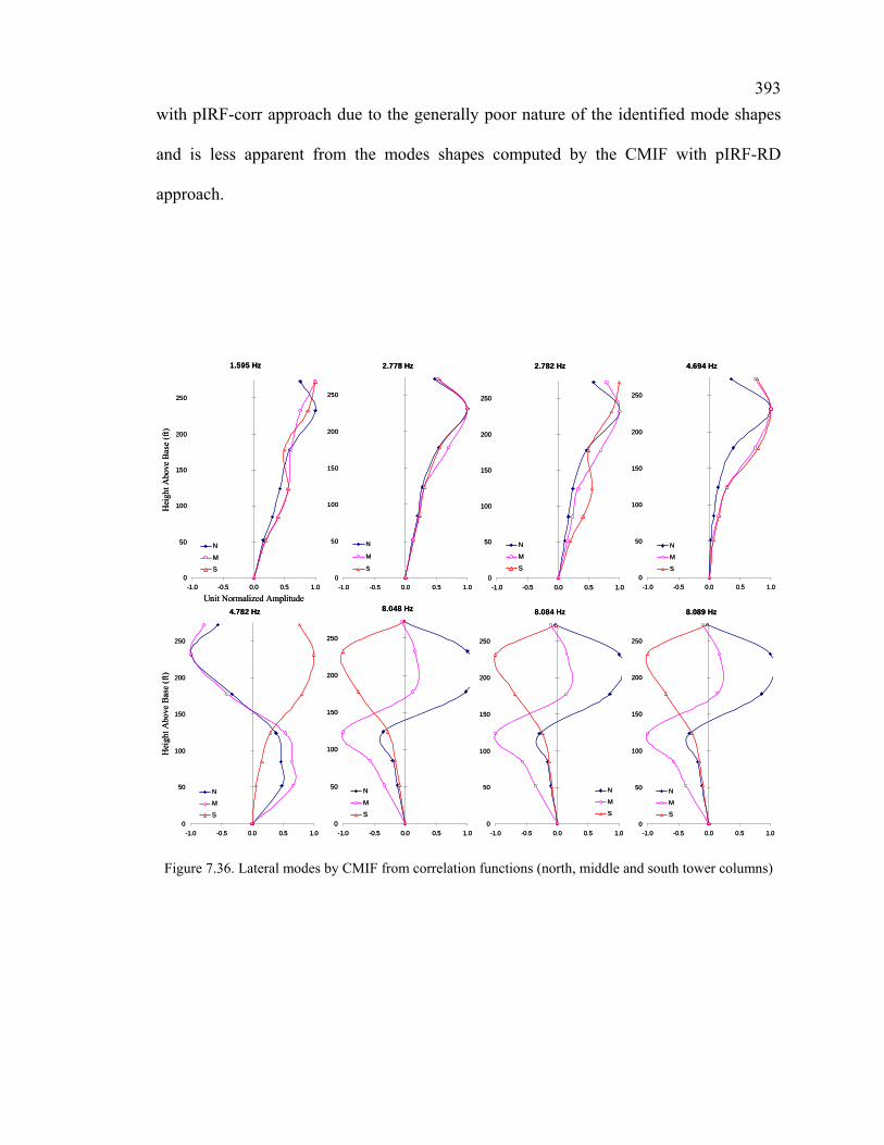
393

with pIRF-corr approach due to the generally poor nature of the identified mode shapes

and is less apparent from the modes shapes computed by the CMIF with pIRF-RD

approach.

Hei

ght A

bove

Bas

e (f

t)


Hei

ght A

bove

Bas

e (f

t)

1.595 Hz

0

50

100

150

200

250

-1.0 -0.5 0.0 0.5 1.0

N

M

S

2.782 Hz

0

50

100

150

200

250

-1.0 -0.5 0.0 0.5 1.0

N

M

S

2.778 Hz

0

50

100

150

200

250

-1.0 -0.5 0.0 0.5 1.0

N

M

S

4.694 Hz

0

50

100

150

200

250

-1.0 -0.5 0.0 0.5 1.0

N

M

S

4.782 Hz

0

50

100

150

200

250

-1.0 -0.5 0.0 0.5 1.0

N

M

S

8.084 Hz

0

50

100

150

200

250

-1.0 -0.5 0.0 0.5 1.0

N

M

S

8.089 Hz

0

50

100

150

200

250

-1.0 -0.5 0.0 0.5 1.0

N

M

S

8.048 Hz

0

50

100

150

200

250

-1.0 -0.5 0.0 0.5 1.0

N

M

S

Hei

ght A

bove

Bas

e (f

t)


Hei

ght A

bove

Bas

e (f

t)

1.595 Hz

0

50

100

150

200

250

-1.0 -0.5 0.0 0.5 1.0

N

M

S

2.782 Hz

0

50

100

150

200

250

-1.0 -0.5 0.0 0.5 1.0

N

M

S

2.778 Hz

0

50

100

150

200

250

-1.0 -0.5 0.0 0.5 1.0

N

M

S

4.694 Hz

0

50

100

150

200

250

-1.0 -0.5 0.0 0.5 1.0

N

M

S

4.782 Hz

0

50

100

150

200

250

-1.0 -0.5 0.0 0.5 1.0

N

M

S

8.084 Hz

0

50

100

150

200

250

-1.0 -0.5 0.0 0.5 1.0

N

M

S

8.089 Hz

0

50

100

150

200

250

-1.0 -0.5 0.0 0.5 1.0

N

M

S

8.048 Hz

0

50

100

150

200

250

-1.0 -0.5 0.0 0.5 1.0

N

M

S

Figure 7.36. Lateral modes by CMIF from correlation functions (north, middle and south tower columns)

394

8.634 Hz

0

50

100

150

200

250

-1.0 -0.5 0.0 0.5 1.0

N

M

S

9.633 Hz

0

50

100

150

200

250

-1.0 -0.5 0.0 0.5 1.0

N

M

S

9.441 Hz

0

50

100

150

200

250

-1.0 -0.5 0.0 0.5 1.0

N

M

S

9.415 Hz

0

50

100

150

200

250

-1.0 -0.5 0.0 0.5 1.0

N

M

S

9.408 Hz

0

50

100

150

200

250

-1.0 -0.5 0.0 0.5 1.0

N

M

S

Hei

ght A

bove

Bas

e (f

t)


Hei

ght A

bove

Bas

e (f

t)

Figure 7.37. Lateral modes by CMIF from correlation functions (north, middle and south tower columns)

395

1.597 Hz

0

50

100

150

200

250

-1.0 -0.5 0.0 0.5 1.0

N

M

S

2.775 Hz

0

50

100

150

200

250

-1.0 -0.5 0.0 0.5 1.0

N

M

S

2.774 Hz

0

50

100

150

200

250

-1.0 -0.5 0.0 0.5 1.0

N

M

S

4.447 Hz

0

50

100

150

200

250

-1.0 -0.5 0.0 0.5 1.0

N

M

S

4.521 Hz

0

50

100

150

200

250

-1.0 -0.5 0.0 0.5 1.0

N

M

S

4.665 Hz

0

50

100

150

200

250

-1.0 -0.5 0.0 0.5 1.0

N

M

S

4.779 Hz

0

50

100

150

200

250

-1.0 -0.5 0.0 0.5 1.0

N

M

S

5.024 Hz

0

50

100

150

200

250

-1.0 -0.5 0.0 0.5 1.0

N

M

S

Hei

ght A

bove

Bas

e (f

t)


Hei

ght A

bove

Bas

e (f

t)

Figure 7.38. Lateral modes by CMIF from random decrement functions (north, middle and south tower columns)

396

6.612 Hz

0

50

100

150

200

250

-1.0 -0.5 0.0 0.5 1.0

N

M

S

8.093 Hz

0

50

100

150

200

250

-1.0 -0.5 0.0 0.5 1.0

N

M

S

8.057 Hz

0

50

100

150

200

250

-1.0 -0.5 0.0 0.5 1.0

N

M

S

8.598 Hz

0

50

100

150

200

250

-1.0 -0.5 0.0 0.5 1.0

N

M

S

9.616 Hz

0

50

100

150

200

250

-1.0 -0.5 0.0 0.5 1.0

N

M

S

9.382 Hz

0

50

100

150

200

250

-1.0 -0.5 0.0 0.5 1.0

N

M

S

Hei

ght A

bove

Bas

e (f

t)


Hei

ght A

bove

Bas

e (f

t)

Figure 7.39. Lateral modes by CMIF from random decrement functions (north, middle and south tower columns)

397

7.5 Discussion

The ambient vibration measurements from the Brooklyn Bridge were analyzed using

the PP, SSI, PTD and CMIF methods to identify the natural frequencies and mode shapes

in the longitudinal, torsional and lateral vibration response directions. Each of the

methods used with the ambient vibration measurement data identified results that could

be considered as spurious even though best practices were employed with the application

of each method. The principal challenge in analyzing the ambient vibration

measurements was related to extracting a relatively small number of natural frequencies

and mode shapes from the much larger pool of identification results for each pure

vibration response direction.

7.5.1 Effectiveness of the Automated Peak Picking Procedure

The automated peak picking procedure that was previously applied to a cantilever

beam specimen as described in Chapter 6 was also used for identifying the dynamic

properties of the Brooklyn Tower. Three different Mode Indicator Functions (MIFs) were

used in conjunction with the automated peak identification procedure, including the

multiple-reference SSCSD MIF. All three functions led to the identification of a similar

quantity of spectral peaks. Furthermore, there were only slight differences between the

locations of the spectral peaks identified from each MIF for a given selection criteria.

This is similar to what was observed in Chapter 6 with the cantilever beam. The spectral

peaks identified from the SSCSD function were generally very similar to those identified

by the other two MIFs, and this indicates that the multiple reference nature of this

function by itself did not significantly add to the quality of the identification results for

398

this particular structure. This MIF may prove to be more effective than the other MIFs for

a more complex structure than the masonry tower that was characterized in this study.

The application of a minimum amplitude level threshold criterion led to a significant

reduction in the number of spectral peaks identified by each MIF. The percent reduction

in the number of identified spectral peaks from the case where no amplitude threshold

was applied was generally very similar for all three MIFs. The only exception to this was

with the ANPSD function in the longitudinal vibration response direction. Because the

SPSD function is essentially the same as the ANPSD function without the normalization

and averaging applied, and the averaging operation is equivalent to dividing the MIF by

the a constant at every frequency line, it is clear that the normalization procedure

somewhat reduced the effectiveness of the minimum amplitude level threshold criterion

for reducing the number of spectral peaks identified by the ANPSD function in this

response direction. The specification of the minimum amplitude level threshold for each

MIF generally permitted the spectral peaks with associated with the highest signal-to-

noise ratios (the most reliable results) to be identified. Some of the identified spectral

peaks were later determined to be associated with the modes of the structure while others

were determined to be spurious results by evaluating different parameters or

characteristics that were produced by the peak picking identification procedure employed

for this study.

399

7.5.2 Identification of the Tower Modes from Peak Picking Results

The most likely candidates for the tower modes in each of the three primary response

directions (longitudinal, torsional, and lateral) were extracted from the sets of spectral

peaks that were identified by applying an automated peak identification procedure to each

response direction for the Brooklyn Tower. Several different parameters and

characteristics that were associated with each of the identified spectral peaks were

subsequently evaluated to extract the most likely candidates for the pure tower modes

from the initial identification results.

The results presented in Chapter 5 from the idealized analytical model of the bridge

served as an essential guide for this process since it permitted the expected dynamic

behavior for the towers to be characterized in terms of the number of tower modes for the

frequency range considered, the order of these modes, and the nature of the expected

mode shapes. The idealized analytical model also provided a necessary conceptual basis

for interpreting the dynamic interactions between the towers and the spans for this

weakly-coupled dynamic system. It would have been impossible to obtain any

meaningful interpretation of the measurement results without first considering the

analytical model results because of the dynamic interactions between the principal

subcomponents of the bridge and the dynamic behavior of the global structural system

were very complex, and because the instrumentation scheme employed for this particular

study was not sufficient to permit these complexities to be completely characterized and

understood by only considering the experimental results.

The process used for evaluating the initial set of peak picking results incorporated

parameters and characteristics derived from both the experimental results and the

400

idealized analytical model results. The experimental results included parameters and

characteristics that were derived from the complete set of spatially distributed reference

locations on the Brooklyn Tower and the outputs from both the towers and spans. The

parameters and characteristics derived from the experimental results that were considered

for the evaluation of the identified spectral peaks included the amplitude of the MIF, the

nature of the operating deflection shapes, the coherence between the tower references and

the tower responses for the same response direction, the coherence between the tower

references in a given direction and the responses of the towers and spans in all directions,

and the unmodified phase information between each tower reference and the tower

responses. The tower mode shape vectors from the idealized analytical model were also

compared with the experimentally determined operating deflection shapes.

The nature of the operating deflection shapes was evaluated by considering the

uniqueness of the deflection shapes associated with different spectral peaks, the physical

plausibility of the shapes for the structure being tested, the visual consistency of the

operating deflection shapes from each reference location for a given spectral peak, the

numerical correlation between the operating shape vectors for the different reference

locations for a given spectral peak, and the correlation between the operating deflection

shapes from all references with each analytical mode shape. Most of the evaluations for

the operating deflection shapes may be considered as multiple reference techniques as

they considered the results from all possible reference locations.

The vibration experiments that were performed on the mechanically transparent

cantilever beam as described in Chapter 6 indicated that the operating deflection shapes

for all of the reference locations of a simple cantilever type structure will be visually

401

consistent with each other at the natural frequencies of the structure. The resonant nature

of the oscillations at these frequencies maximizes the signal-to-noise ratios in the

measurements, and even when the selected reference location was associated with

minimal vibration response amplitudes (the clamped support), the operating deflection

shapes computed from this reference location still agreed with those computed from other

reference locations associated with much more significant vibration amplitudes. This

observation is somewhat inconsistent with standard best practices for experimental modal

testing (i.e. placing sensors at the locations of nodal points); however, the experimental

noise that is invariably present in the response of such sensors noise appears to have

mitigated the problem with dividing the responses by a zero value.

Evaluating the visual consistency between the operating deflection shapes at each

identified frequency was a very effective tool for excluding many of the spurious peaks

from the identification results. This evaluation approach also provides a subjective

measure of the uncertainty associated with each spectral peak that is often less obvious

from the numerical measures of the consistency between the operating deflection shapes

from different reference locations. When all of the operating deflection shapes are not

exactly consistent with each other, it may be observed that the signal-to-noise ratios for

the measurements are not maximums. In Chapter 6, this behavior was typically observed

as the natural frequency was approached but not quite reached in the identified results, or

more commonly when there was not sufficient ambient dynamic excitation energy

supplied to the frequency to permit its reliable identification. Finally, this evaluation

approach for the operating deflection shapes acts as a roadmap for locating the sources of

experimental uncertainty in the results. If the operating deflection shape associated with a

402

particular reference locations is not visually consistent with the shapes from the other

reference locations, the uncertainty may be assigned to the reference location that

produced the inconsistent operating deflection shape. The value of this approach for

identifying spurious results, even when it is implemented on a limited basis, was

demonstrated with lateral vibration responses of the Brooklyn Tower for all of the

identification methods used in this study. In this case, evaluating the visual consistency of

the operating deflection shapes and the mode shapes that were generated for the three

columns of the tower was shown to be effective for ruling out spurious results.

It should be noted that it was only possible to evaluate the consistency of the

operating deflection shapes for different references in the peak picking approach because

a stationary instrumentation scheme was employed for ambient vibration measurements.

Most of the ambient vibration tests that have been previously performed on major long

span bridges and other large constructed systems have employed a roving instrumentation

scheme. This is typically done to obtain a finer resolution for the identified mode shapes,

and to permit the vibration test to be conducted quickly using a small number of

accelerometers. The use of a roving instrumentation scheme may be perfectly adequate

for characterizing very flexible structures or structural components that are well excited;

however, in cases where the vibration responses are very small and the ambient dynamic

excitation level is low, a roving instrumentation scheme precludes the use of multiple and

spatially distributed references for the modal identification. It also does not permit the

operating deflection shapes from multiple and spatially distributed references to be

compared. This has been shown to be a very useful tool for excluding spurious results

and ensuring a more reliable modal identification. The relative merits of mode shape

403

resolution and testing speed for the roving scheme versus the capability to conduct a

more reliable identification with a stationary instrumentation scheme should be carefully

considered when designing an ambient vibration experiment for a large constructed

system. It should also be noted that the visually consistency of the shapes is not sufficient

by itself for identifying the pure tower modes, since the shapes may be consistent but

implausible, or they may be consistent at spectral peaks that are associated with peaks in

the excitation spectra as was observed in Chapter 6 with the cantilever beam.

The full set of evaluation results for the different parameters associated with each

spectral peak generally supported the selection of the spectral peak with the largest MIF

amplitude in a given shape type group as the most likely mode of the structure. In the few

cases where the amplitude of the MIF was very similar at more than frequency within the

same operating deflection shape type group, there was more uncertainty associated with

identifying the most likely mode. Furthermore, the results obtained by evaluating the

other parameters in these cases were often very comparable or sometimes contradicted

each other. This reduced the effectiveness of these evaluations for selecting the most

likely tower modes. The MIF amplitude was generally assigned the greatest importance

for selecting the likely tower mode for these cases; however, this does not mitigate the

uncertainty associated with the identification of these modes. This uncertainty could

possibly be mitigated by considering the results from a more detailed analytical model of

the bridge; however, the uncertainty associated with any analytical model may offset the

effectiveness of such a comparison. Performing a forced vibration test where adequate

dynamic excitation is supplied in the range of these frequencies would also mitigate the

uncertainty associated with the identification of these modes.

404

The frequencies and operating deflection shapes that may be considered as the most

likely modes of the Brooklyn Tower as determined by evaluating the parameters and

characteristics associated with peak picking results are shown in Figure 7.40 and Figure

7.41. The uncertainty associated with the fundamental mode in each of the three response

directions was relatively low based on the spectrum of evaluation results for each

frequency. The uncertainty associated with the 2nd pure longitudinal, torsional, and lateral

modes identified for the Brooklyn Tower was much greater and this is uncertainty is most

likely the result of limitations of the ambient vibration test method for characterizing

modes that are near to or beyond the upper end of the effective frequency band for the

ambient dynamic excitation.

The span identification results from an earlier investigation of the bridge, and the

measurements from the very limited array of span sensors used in conjunction with the

tower characterization were considered as part of the evaluation process for identifying

the most likely tower modes. These results proved to be somewhat inadequate and

incomplete, especially at the higher end of the frequency band of interest, for

significantly reducing the uncertainty related to identifying the most likely tower modes.

The objectives and frequency band of interest for the previous span investigation were

different from the those associated with the tower characterization, and these differences

significantly limited the usefulness of the span identification results for evaluating and

interpreting the tower measurements. Furthermore, the span instrumentation that was

permitted for the ambient testing of the towers was too limited to perform a meaningful

identification of the spans for the full frequency band of interest for the towers. This

deficiency was the related to the design of the experiments and not the measurements

405

themselves. It also demonstrates that trying to merge the results from independent

characterizations of different bridge components in a weakly-coupled dynamic system is

not very meaningful, particularly if the objectives for the characterizations are not the

same.

406

0

50

100

150

200

250

-1.0 -0.5 0.0 0.5 1.0

Blong

Clong

Elong

Glong

Hlong

0

50

100

150

200

250

-1.0 -0.5 0.0 0.5 1.0

Blong

Clong

Elong

Glong

Hlong

1st Longitudinal = 1.387 Hz 1st Torsional = 2.695 Hz

0

50

100

150

200

250

-1.5 -1.0 -0.5 0.0 0.5 1.0 1.5

B LAT

C LAT

E LAT

FN LAT

GN LAT

HLAT

0

50

100

150

200

250

-1.5 -1.0 -0.5 0.0 0.5 1.0 1.5

B LAT

C LAT

E LAT

FN LAT

GN LAT

HLAT

0

50

100

150

200

250

-1.5 -1.0 -0.5 0.0 0.5 1.0 1.5

B LAT

C LAT

E LAT

FN LAT

GN LAT

HLAT

North Middle South

1st Lateral = 1.597 Hz

Figure 7.40. Brooklyn Tower modes from PP – 1st Longitudinal, 1st Lateral and 1st Torsional

407

0

50

100

150

200

250

-1.5 -1.0 -0.5 0.0 0.5 1.0 1.5

B LAT

C LAT

E LAT

FN LAT

GN LAT

HLAT

0

50

100

150

200

250

-1.5 -1.0 -0.5 0.0 0.5 1.0 1.5

B LAT

C LAT

E LAT

FN LAT

GN LAT

HLAT

0

50

100

150

200

250

-1.5 -1.0 -0.5 0.0 0.5 1.0 1.5

B LAT

C LAT

E LAT

FN LAT

GN LAT

HLAT

North Middle South

0

50

100

150

200

250

-1.0 -0.5 0.0 0.5 1.0

Blong

Clong

Elong

Glong

Hlong

0

50

100

150

200

250

-1.0 -0.5 0.0 0.5 1.0

Blong

Clong

Elong

Glong

Hlong

2nd Longitudinal = 3.765 Hz 2nd Torsional = 7.051 Hz

2nd Lateral = 4.766 Hz

0

50

100

150

200

250

-1.5 -1.0 -0.5 0.0 0.5 1.0 1.5

B LAT

C LAT

E LAT

FN LAT

GN LAT

HLAT

0

50

100

150

200

250

-1.5 -1.0 -0.5 0.0 0.5 1.0 1.5

B LAT

C LAT

E LAT

FN LAT

GN LAT

HLAT

0

50

100

150

200

250

-1.5 -1.0 -0.5 0.0 0.5 1.0 1.5

B LAT

C LAT

E LAT

FN LAT

GN LAT

HLAT

0

50

100

150

200

250

-1.5 -1.0 -0.5 0.0 0.5 1.0 1.5

B LAT

C LAT

E LAT

FN LAT

GN LAT

HLAT

0

50

100

150

200

250

-1.5 -1.0 -0.5 0.0 0.5 1.0 1.5

B LAT

C LAT

E LAT

FN LAT

GN LAT

HLAT

0

50

100

150

200

250

-1.5 -1.0 -0.5 0.0 0.5 1.0 1.5

B LAT

C LAT

E LAT

FN LAT

GN LAT

HLAT

North Middle South

0

50

100

150

200

250

-1.0 -0.5 0.0 0.5 1.0

Blong

Clong

Elong

Glong

Hlong

0

50

100

150

200

250

-1.0 -0.5 0.0 0.5 1.0

Blong

Clong

Elong

Glong

Hlong


0

50

100

150

200

250

-1.0 -0.5 0.0 0.5 1.0

Blong

Clong

Elong

Glong

Hlong

0

50

100

150

200

250

-1.0 -0.5 0.0 0.5 1.0

Blong

Clong

Elong

Glong

Hlong


2nd Lateral = 4.766 Hz

Figure 7.41. Brooklyn Tower modes from PP – 2nd Longitudinal, 2nd Lateral and 2nd Torsional

7.5.3 Performance of the Advanced Modal Identification Methods

A number of more advanced, multiple-reference modal identification techniques were

applied to the ambient vibration measurements from the Brooklyn Tower. These

techniques included the SSI method, the PTD method, and the CMIF method. Pseudo

impulse response functions were estimated from the ambient vibration measurements by

408

using correlation functions and Random Decrement functions, and these were used with

the PTD (time domain) and CMIF (frequency domain transformation of the pIRF)

methods. These identification methods generally did not offer any significant

improvement over the results that were obtained by the peak picking method

implemented for this study. In many cases, these methods actually provided results that

were less reliable or meaningful than the results obtained from peak picking. All three

methods identified various numbers of spurious results as tower modes. The

identification results from these methods also did not always include the frequencies and

mode shapes that were identified from peak picking as the most likely tower modes.

It was generally difficult to separate the tower modes from the spurious modes

identified by each method by considering only frequencies and mode shape results

produced by each method. This was primarily because these methods identified only one

mode shape for each frequency, even when multiple references were used for each

method. This would not be an issue if these methods did not identify any spurious results,

but since all of them clearly did, a single mode shape was often not adequate for

identifying the spurious results. The analysis of the lateral tower responses by these

methods produced multiple mode shapes (one for each of the three tower columns) which

could be visually compared with each other for the identified modes. Comparing the

modes shapes for each tower column permitted many of the spurious identification results

to be identified and excluded. Each of these multiple-reference methods could be applied

for single reference locations, and the identification process could be repeated for all of

the possible reference locations in order to generate a set of mode shapes that could be

compared with each other; however, there would likely be significant variation in the

409

identification results for each reference locations used. This would in turn limit the

effectiveness of comparing the mode shapes associated with each reference location for

identifying any spurious results. In this study, the spurious results from these methods

were identified by comparing them with the significantly more transparent results

obtained by the peak picking method.

The effectiveness of each of these identification methods varied somewhat depending

on the tower response direction that was being analyzed. The SSI identification results

included the two frequencies and mode shapes identified as the most likely tower modes

by peak picking in the longitudinal and lateral response directions, but only the first mode

in the torsional response direction. The PTD identification results using the pIRF-corr

approach included the two longitudinal frequencies and mode shapes, the two torsional

natural frequencies and the first torsional mode shape, but none of the lateral tower

modes. The PTD identification results using the pIRF-RD approach included the two

longitudinal natural frequencies but the corresponding mode shapes were poor. This

approach did identify the two modes and their correct shapes in the lateral and torsional

response directions. The CMIF identification results using both the pIRF-corr and pIRF-

RD approaches did not include the two longitudinal natural frequencies or their mode

shapes. The CMIF identification results using the pIRF-corr approach did not include the

two torsional or lateral frequencies and their mode shapes, but the results using the pIRF-

RD approach did. It may be observed that the pIRF functions developed from Random

Decrement functions produced slightly better results with the PTD and CMIF methods

than the pIRF functions that were estimated from the correlation functions. The SSI

method also produced the most consistent results of the three methods for all of the tower

410

response directions. None of these methods produced results that were inherently better

than those identified by the peak picking method used for this study.

411

CHAPTER 8: CONCLUSIONS AND FUTURE WORK

8.1 Introduction

The focus of this thesis was the experimental characterization of the towers in cable-

supported bridges by ambient vibration testing. The experimental characterization

requires that the tower modes and their corresponding mode shapes are extracted from

ambient vibration measurements. A number of challenges and unresolved issues were

encountered while trying to experimentally characterize the dynamic properties of a

tower from a major suspension bridge. This thesis was designed in an attempt to address

some of the most critical of these unresolved challenges. A series of experimental and

analytical studies were designed and conducted with the following objectives related to

these unresolved challenges:

• Define Fundamental Dynamic Behavior: The global structural system

consisting of a very stiff and massive subcomponent (masonry tower) and a very

flexible and light subcomponent (spans) were studied using an idealized analytical

model. The dynamic interactions of the tower and span components were

investigated to determine if pure modes exist for each component, to determine if

there are coupled modes consistent with simultaneous resonance of the tower and

span components or simultaneous resonance of the tower component in more than

one response direction, and to evaluate the character of the tower modes. The

most critical responses of the tower are investigated to determine what

identification results from the experiment should be classified as the tower modes.

412

• Ambient Dynamic Excitation Characteristics: The ambient dynamic excitation

acting on the tower components of the bridge is of a very different nature than

what is generally assumed in ambient vibration testing. The ambient dynamic

excitation acting on the towers also has a fundamentally different character from

that which acts on the flexible spans. The possible effects of this excitation

complexity on the effectiveness of different identification methods and on the

accuracy and reliability of the identified properties were systematically

investigated using a mechanically transparent beam that was subjected to

“ambient dynamic excitation” with well-defined characteristics.

• Effectiveness of Different Modal Identification Methods: The interactions of

between the spans and towers lead to many peaks in the output spectra for the

towers that are not necessarily associated with the resonant responses of the

towers. Several frequency domain and time domain modal identification methods

are evaluated for the tower identification problem to determine if any of these

methods provides a more reliable identification of the resonant frequencies and

mode shapes of the towers. The conventional single reference peak picking

method is compared with an enhanced peak picking approach that incorporates

multiple reference locations, and with more sophisticated identification

algorithms that also incorporate multiple references. The different identification

methods are applied and evaluated for the characterization of a mechanically

transparent cantilever beam subject to ambient dynamic excitation of various

degrees of complexity, and for the ambient vibration responses of a tower from

the Brooklyn Bridge. Finally, a number of parameters developed from the

413

multiple reference locations are investigated for extracting the tower responses

most likely due to resonance from those associated with interactions of the

structural components (spans and towers) and those which represent spurious

results.

• Experiment Design: The most reliable experimental approach for characterizing

the modal properties for the tower in a cable-supported bridge is investigated. The

modal identification using the traditional peak picking approach is compared with

the modal identification using an improved peak picking approach and by more

sophisticated modal identification methods. The results obtained from the use of a

single reference location are compared with those using multiple reference

locations to determine if this leads to any improvement in the reliability of the

identified properties. It appears that in all of the ambient vibration tests that have

previously been undertaken to characterize the dynamic properties of the towers

in a cable-supported bridge have utilized a roving instrumentation scheme with a

single reference location. The majority of these structures have been identified

using the peak picking method with only a single reference location. The

identification results and ambient vibration measurements from the spans are also

considered in conjunction with the identification of the tower to evaluate if the

span measurements improve the reliability of the tower identification.

The conclusions that can be made with respect to the individual objectives described

above are presented in the following sections. Specific conclusions related to the

individual analytical and experimental studies conducted to address these objectives may

be found in the discussion sections of the chapters describing each study.

414

8.2 Fundamental Dynamic Behavior for a Tower in a Cable-Supported Bridge

The fundamental dynamic behavior for the tower components in a cable supported

bridge was evaluated in the context of idealized analytical models of the Brooklyn

Bridge, and through analysis of the experimental results. These studies indicate that

resonant modes associated with the tower remain distinct when the tower is integrated

with the rest of the structure. In other words, the same resonant modes that were

identified for the free-standing towers were also identified in the model that included

representations of the other bridge components (spans, main cables, stay cables). The

frequencies at which the tower modes occurred changed slightly between the different

model cases; however, the modal configurations (mode shapes) associated with the

resonant modes of the tower were consistent in each of the model cases considered. The

resonant modes of the tower identified from the free standing analysis case could be

tracked through all of the subsequent analysis cases. These particular tower modes were

associated with the maximum responses observed for the towers. Furthermore, the towers

were observed to participate in some of the modes associated with the spans, and the unit

normalized mode shape of the tower at these frequencies was very similar to its unit

normalized mode shape for the resonant modes associated with the tower. The non-

normalized amplitude of the tower’s modal configuration in the span modes was

significantly smaller than its non-normalized amplitude in the tower modes. It is clear

that the level of the tower’s response was more critical in the modes associated with the

towers than in the modes associated with the spans. The tower was also observed to

respond in all three directions at every mode identified, although the response was

generally dominant in only one response direction. The simultaneous responses in the

415

other tower directions were generally very minor and should be considered as incidental

to the response in the dominant direction.

It is clear from the discussion above that pure tower modes can exist in a cable-

supported bridge, and that these modes represent the most critical responses of the tower.

The tower may experience oscillations with a similar modal configuration to the pure

tower modes; however, these oscillations are not really meaningful they are significantly

smaller than the tower responses for the pure tower modes. There were no tower-span

coupled modes identified in the model in which the response of the tower and the spans

were both larger than the response of either component in the modes associated with that

component. The focus of the experimental characterization of the towers in a cable-

supported bridge should be the pure tower modes since they are associated with the

maximum responses. The other motions of the tower that occur as a result of the physical

connections between the different bridge components are less meaningful and their

inclusion in the identification results may serve to obscure the more critical tower results.

The pure tower modes represent the only identification results that should be associated

with resonance of the towers, and for which mode shapes and damping ratios will be

meaningful. The use of an idealized analytical model was found to be a transparent and

effective approach for locating and tracking the critical pure tower modes in the dynamic

response of the complete structure.

The results from the study of the idealized analytical model also suggest that there

may be five different classes of possible response for the towers and spans in a cable-

supported bridge. Furthermore, these different classes of response depend on the nature

of the loading applied to the structure, the physical properties (mass, stiffness, damping)

416

of the different bridge component, and the physical connections between the individual

components. The different levels or classifications of possible response may be described

as follows:

• Class 1 Response: A static load applied to the spans will produce static

deflections of the spans and towers (since they are physically connected to each

other).

• Class 2 Response: A forcing function applied to the spans will produce time

varying deflections for both the spans and towers. The deflections of both

components will not be amplified compared to the equivalent static response if the

forcing function is not at or near a natural frequency of the spans or tower.


varying deflections for both the spans and towers. If the frequency of the forcing

function is at or near a natural frequency of the span, but not at or near a natural

frequency of the tower (pure tower mode), the span will resonate (dynamic

amplification of the span deflection). The time varying deflection of the tower

will also be amplified, but this amplification is the result of the amplified loading

from the resonating spans. Because the response of the tower in this case is due to

amplified loads acting on it, it is not very meaningful to identify the damping ratio

associated with the tower’s response.



function is at or near a natural frequency of the tower (pure tower mode), but not

417

at or near a natural frequency of the span, the tower will resonate (dynamic

amplification of the tower deflection). The time varying deflection of the span

may also be amplified, but this amplification will be the result of the amplified

motions of the resonating tower.



function is at or near a natural frequency of the span and tower (pure tower

mode), the span will resonate (dynamic amplification of the span deflection) and

the tower will resonate (dynamic amplification of the tower deflection). This will

only occur if the natural frequency of the span is close to the natural frequency of

the tower. This condition would be associated with a coupled tower-span mode (a

global structural mode), since the tower and span would experience simultaneous

resonant oscillations. It should be noted that this condition was not observed in

the results from the idealized analytical model of the Brooklyn Bridge.

The different levels of response described above are very relevant for the

experimental characterization of the towers in a cable-supported bridge, since the tower

responses associated with Class 2 – Class 5 will be reflected as peaks in the output

spectra for the tower sensors, and the span responses associated with Classes 2 – 5 for

will appear as peaks in the excitation spectrum for the tower. The peaks in the excitation

spectrum for the tower will appear as peaks in the output response spectra for the tower.

It should be noted that since the towers in the Brooklyn Bridge are very stiff in relation to

the spans, the peaks in the output spectra due to the peaks in the excitation spectra may be

of a similar magnitude. It should be noted that the influence of the spans on the towers

418

(amplified loads due to span modes) will be most pronounced at the frequencies

associated with the lower vertical modes due to the larger antinodes in the span mode

shapes at these frequencies. The influence will also be most pronounced for the

longitudinal/torsional motions of the tower when traffic is the primary source of

excitation for the spans. The ambient vibration measurements recorded from the

Brooklyn Bridge tower also reflected these findings.

It should be noted that the peaks in the output spectra associated with the various

interactions and different responses described above will be in addition to any spurious

peaks due to noise or other experimental errors. The presence of a significant number of

spectral peaks in the output spectra for the tower that are all not necessarily associated

with the resonant response of the tower (pure tower modes) represents the most

significant barrier to identifying the pure tower modes from the ambient vibration

measurements.

8.3 Character of the Ambient Dynamic Excitation

The ambient dynamic excitation is assumed to be Gaussian white noise for the

purpose of characterizing the modal properties of a structure by ambient vibration testing.

It is generally assumed that the nature of the ambient dynamic excitation will not

conform to the normally assumed characteristics. Furthermore, it was shown in the

previous section that the ambient dynamic excitation spectrum for the tower will contain

peaks associated with the vibrations of the spans. The effective frequency bandwidth of

the ambient excitation is generally not well-characterized since the input is unmeasured.

Finally, the ambient dynamic excitation acting on the tower will often be spatially

419

localized whereas it is spatially well-distributed on the spans (in the case of traffic related

dynamic excitation).

A number of controlled excitation cases were designed and applied to a mechanically

transparent cantilever beam to evaluate the effects of the excitation characteristics on the

identified modal properties. The principal excitation characteristics considered included

random excitation with a range of effective frequency bandwidths. The frequency band of

the random excitation applied to the cantilever beam included a broad band case that

encompassed the entire frequency band of interest for the specimen and narrow band

cases that encompassed various fractions of the entire frequency band of interest. The

random excitation cases were also repeated with a known harmonic excitation component

superimposed on the excitation spectrum. The dynamic excitation from each of these

cases was transmitted to the structure through its clamped end. A narrow band excitation

case that was spatially distributed along the span of the cantilever beam was also

evaluated as a separate case. Finally, an excitation case that contained a pure harmonic

component was applied to the beam (transmitted through its clamped end). Several

different modal identification methods were used to estimate the modal properties of the

beam from each excitation case. The dynamic excitation applied to the cantilever beam

for each excitation case that was considered was treated as unmeasured ambient dynamic

excitation for the subsequent modal identification of the beam.

The output spectra from each of the random excitation cases included many spurious

peaks in addition to peaks that corresponded to the natural frequencies of the beam. The

modal properties identified by the peak picking method from the pure random excitation

cases did not show that the identification results were significantly affected by the

420

frequency band of the input. The first four natural frequencies of the beam could be

extracted from each of the pure random excitation cases. The accuracy of the

identification of the higher modes that were identified was somewhat diminished for the

pure random excitation cases with narrow effective frequency bandwidths. The frequency

range of the accelerometers used in this study was zero to 150 Hz for the most accurate

performance, and because the upper limit is less than the frequency of the 4th and 5th

modes of the cantilever, some inaccuracy was expected for the identification of these

modes.

The first five modes were identified from the random excitation cases with the

harmonic excitation component, and the identification results from the peak picking

approach were more consistent for all of these excitation cases. This indicates that the

nature of the excitation energy supplied by the eccentric mass shaker (low frequency

harmonic) was fundamentally transformed as it was transmitted across the clamped

support. The harmonic nature of the excitation was identified from the output responses

of the cantilever sensors; however, enough energy from the excitation was leaked across

the frequency band of interest to permit all five modes of the beam to be consistently

identified. This is particularly evident from the results of the excitation case that only

included the harmonic excitation. The identified modes from that excitation case were

still consistent with the modes identified from the random excitation cases with

superimposed harmonic excitation. This is an important finding in that it demonstrates

that the transmitted excitation due to an applied harmonic excitation may be spread

across the frequency band of interest. In other words, harmonic excitation may assume

broad banded excitation characteristics as it is transmitted through the different structural

421

components. This has important implications for the subsequent modal identification of a

structural component (such as a tower in a cable-supported bridge) as the harmonic

components of the ambient dynamic excitation acting on the towers that is caused by the

resonant oscillations of the spans may distribute its energy across a wider frequency band

as it is transmitted to the towers.

8.4 Effectiveness of Different Modal Identification Methods

The effectiveness of several different modal identification methods was compared

and evaluated for the case of ambient vibration measurements using a mechanically

transparent cantilever beam (dynamic properties have low uncertainty) in the laboratory

and for identifying the modal properties of a tower in the Brooklyn Bridge. The

identification methods that were evaluated included the conventional peak picking

identification approach used for roving instrumentation schemes and in which a single

reference location is used in conjunction with the modal identification, a peak picking

approach that was modified to incorporate the multiple reference locations available

when a stationary instrumentation scheme is used for the ambient vibration test, and

several multiple reference time domain and frequency domain methods. The time domain

methods included the Stochastic Subspace Identification (SSI) method and the

Polyreference Time Domain (PTD) method, and the other frequency domain

identification method used was the Complex Mode Indicator Function (CMIF) method.

The application of these different identification methods with the mechanically

transparent cantilever beam indicated that all methods led to the identification of

numerous frequencies that were not associated with the modes of the cantilever. The

422

results from each method included various numbers of spurious results in addition to the

natural frequencies of the cantilever. In the cases where a harmonic excitation was

applied to the beam, the excitation was included with the modal identification results.

The peak picking results indicated that the number of frequencies identified by the

automated peak identification procedure was more a function of the number of spectral

lines considered when identifying the peaks than the particular mode indicator function

that is used to identify the peaks. The use of a minimum amplitude threshold in

conjunction with the automated peak identification procedure significantly reduced the

number of spurious peaks that were identified, and because the resulting peaks identified

were associated with the largest response (and signal-to-noise ratios), the identification

results always included the frequencies that corresponded to the modes of the cantilever

beam. In order to extract the modes from the peak picking identification results a process

of elimination approach was used that considered the following characteristics and

parameters associated with the identified spectral peaks:

• Number of theoretical modes in the frequency range considered: Establishing the

expected number of natural frequencies and their mode shapes for the frequency

range considered provides a necessary roadmap for interpreting the identification

results and excluding the results that are least likely to represent the modes of the

structure.

• Physical plausibility of the operating deflection shape: The operating deflection

shapes associated with some of the identified spectral peaks will not be realistic

and can be excluded as a spurious result. A typical example for the cantilever

423

beam was the presence of large antinodes in the operating deflection shape at the

support location.

• Similarity of the operating deflection shapes for different spectral peaks: The

operating deflection shapes associated with different peaks often have very

similar shapes. The frequencies associated with similar operating deflection

shapes can be grouped together and considered in the context of the theoretical

results as possible candidates for the same mode of the structure. A single

frequency from a given shape type group will often represent the most likely

candidate for the theoretical mode that corresponds to the shape type group being

considered.

• Consistency of the operating deflection shapes from different reference locations

at an identified frequency: The unit normalized operating deflection shapes

computed from each reference location were found to be consistent at the peaks

that corresponded to the true natural frequencies of the beam. The operating

deflection shapes from different references were inconsistent if the mode was not

adequately excited, or for spurious peaks. This may be considered as a necessary

condition for the presence of a mode, but it is not a sufficient condition. The

operating deflection shapes from different reference locations were also consistent

for peaks that were due to peaks in the excitation spectra, and at some peaks

related to noise. For example, the operating deflection shapes from different

reference locations were consistent with each other for some identified peaks;

however, the deflection shape was sometimes not consistent with any of the

theoretical mode shapes. Comparing the consistency of the operating shapes from

424

different reference locations is an effective tool for reducing the number of

identified frequencies that may be considered as the possible modes of the

structure. This can also be used as a tool to determine the possible locations of

modes that may not have been adequately excited, and can be used to evaluate the

uncertainty associated with an identified mode in a much more transparent way

than by looking at coherence values. It also provides an indication of the spatial

location (the reference location) of any errors or uncertainty. It is important to

note that the evaluating the consistency of the operating shapes requires that

multiple reference locations are available from the instrumentation scheme.

• Modal Assurance Criterion (MAC) values for operating deflection shapes

associated with different references: This parameter is related to the visual

consistency of the shapes described above, and can be considered as the

numerical equivalent of the visual consistency. It is subject to the same limitations

associated with the visual consistency (e.g. shapes consistent but implausible, and

consistent for peaks due to noise or harmonics in the excitation spectrum). The

MAC parameter may be combined into a single value that reflects the individual

MAC values for each reference location thereby including multiple reference

locations in a single parameter. This parameter may be considered to be less

transparent to interpret than the visual consistency since a minimum value for this

parameter must be established to evaluate whether the peak is a mode or not. This

parameter only indicates if the shapes are consistent with each other, it does not

indicate if the shapes are not realistic.

425

• Amplitude of the peaks within each operating deflection shape type group: The

spectral peak in a given operating deflection shape type group with the largest

amplitude was usually associated with the mode of the structure. This is also a

necessary but insufficient condition for identifying the modes since the largest

identified peaks did not all correspond to the modes of the structure. The peaks

with the largest amplitudes will usually contain the modes of the structure because

of the dynamic amplification of the structural response that occurs at resonance.

• Ordinary Coherence Functions: The ordinary coherence function can be used to

identify the resonant frequencies of the structure. This parameter will be a

maximum at the locations of the resonant frequencies (due to the high signal-to-

noise ratio in the measurements). This may be considered a necessary but

insufficient indicator of resonance since the coherence was also generally large at

peaks associated with noise (the noise was coherent from all of the output

locations) and at peaks associated with peaks in the excitation spectrum.

• MAC values between theoretical mode shapes and operating deflection shapes:

This parameter can be used to identify the results that show good agreement with

the expected results, but this parameter relies on the analytical model being able

to correctly represent the true behavior of the structure. In some cases, this

parameter indicated that the operating deflection shapes associated with a

spurious peak showed better agreement with the theoretical shape than the

operating shapes associated with the actual natural frequency of the system. As a

result, this parameter should not be the only criteria used to extract the modes

426

from the identification results. It may be useful tool for corroborating the modes

identified by considering the other parameters.

• Phase factors: The raw phase factors computed between each output location and

the reference locations were not close to zero or 180 degrees (consistent with

normal mode behavior) at the peaks that were associated with peaks in the

excitation spectrum. The phase factors can be used to help exclude such peaks

from the results; however, evaluating the phase factors is not sufficient by itself to

isolate the natural frequencies from the other spurious results since the phase

factor values at the natural frequencies and at spurious peaks can be close to zero

or 180 degrees.

The modes of the cantilever beam could be identified from the peak picking results by

considering these parameters and characteristics together, however, this evaluation

remains a somewhat subjective process. The natural frequencies and mode shapes could

be identified from the many peaks identified for a simple structure tested in the laboratory

using this approach. In general, the modes could be more confidently identified when

multiple references were used in conjunction with the peak picking method.

The more advanced modal identification algorithms did not prove to be any more

effective or reliable than the peak picking method for identifying the modes. Although

these methods did tend to identify fewer frequencies than the most basic implementation

of the peak picking method (peak identification with no minimum amplitude threshold

criterion), the modes could not be identified from the results without considering the peak

picking results as a guide. Furthermore, the mode shapes estimated by these methods

were often less reliable than those produced by peak picking for the same identified

427

frequency. The SSI method did tend to produce slightly more consistent results than the

PTD and CMIF methods for the different excitation cases that were evaluated.

The different modal identification methods were also applied to characterize the

modal properties of a masonry tower from the Brooklyn Bridge using ambient vibration

measurements. The vibrations of the Brooklyn Tower due to ambient excitation were

evaluated in the longitudinal, torsional, and lateral response directions in an attempt to

identify the pure tower modes (the modes associated with the maximum response). A

significant number of peaks were identified from each of the three principal response

directions using the automated peak picking procedure for several different mode

indicator functions. The number of peaks identified from each of the mode indicator

functions was similar for a given response direction. Based on the dynamic behavior

observed from the analysis of an idealized analytical model of the bridge and the data

analysis for the cantilever beam that was tested using the same experimental setup, the

identified peaks were assumed to include the pure tower modes, amplified tower

responses due to resonant oscillations of the spans or main cables in their modes, tower

responses due to non resonant oscillations of the spans, and spurious results due to

experimental/signal processing errors and noise. The number of identified peaks was

dramatically reduced when a minimum amplitude level threshold was applied to the

initial pool of identified spectral peaks.

The identified peaks were subsequently evaluated for the same characteristics that

were used in conjunction with the cantilever beam test to identify the most likely pure

tower modes for each of the principal response directions. The expected number of pure

tower modes and their order for the frequency range of the experiment was identified

428

from the analysis of the idealized analytical model of the bridge, and this was used as a

guide for extracting the pure tower modes. The modal properties identified for the bridge

spans in a previous study and the vibrations measured at a limited number of locations on

the spans during the tower study were also considered in evaluating the identified spectral

peaks. The peak picking results were estimated using a single reference location as it is

believed that this approach has been used in all of the previous tower characterization

applications, and by using the multiple reference locations that were available from the

stationary instrumentation scheme that was employed for the Brooklyn Bridge study.

The most likely pure tower modes were extracted from the peak picking results by

considering a spectrum of parameters and the characteristics of the operating deflection

shapes that were associated with each identified spectral peak. The individual parameters

considered in the evaluation were modified to incorporate the multiple reference

locations that were available in this study. The term “most likely” is used to describe the

identified pure tower modes in order to reflect the uncertainty that is associated with

these results. It should be noted that this uncertainty is a characteristic of the ambient

vibration test method for this particular application (the tower in a cable supported

structure). This uncertainty represents a combination of the individual uncertainties

associated with the individual parameters and characteristics (the experimental and

analytical results) considered for selecting the pure tower modes. This uncertainty was

also observed to increase for the identification of the higher frequency modes of the

tower. The modal identification of the simple cantilever beam that was tested in a

laboratory and for which the expected results could be established with reasonably good

level of reliability that the experimental parameters that are typically considered

429

(ordinary coherence, phase factors) for extracting the resonant modes from the peak

picking results are necessary but insufficient characteristics to guarantee that only the

actual modes are identified from the peak picking results. Indeed, these particular

parameters may have values that indicate the presence of a resonant frequency where one

does not actually exist (false-positive indications of a mode). The visual consistency of

the operating deflection shapes computed from multiple reference location proved to be

an effective tool for excluding many spurious identification results, and can be credited

with helping to improve the overall efficiency of the identification process and reducing

the uncertainty associated with the identification results to some degree; however, even

this characteristic was shown to sometimes indicate a likely mode for a spurious peak. It

should be noted that the spurious and less critical tower results could be excluded from

the same set of identified peaks with much more confidence when the multiple references

were used (Chapter 7) than when only a single reference location was considered

(Chapter 3).

The modal properties of the spans and the interactions of the spans with the tower

responses were also considered as part of the evaluation process used to extract the pure

tower modes from the identified spectral peaks. The previously identified modal

properties for the spans were of limited value for interpreting the tower results in this

case since the objective of that study was to characterize the spans, and the identified

results only covered a portion of the frequency band associated with the modal properties

of the tower. Furthermore, the span responses measured in conjunction the tower

characterization study were not adequate for characterizing the modal properties of the

spans. The rather limited span measurements were really only adequate to detect the

430

locations of natural frequencies identified in the earlier study. The coherence between the

reference locations on the tower and the output locations on the spans and the Manhattan

Tower could be used to corroborate the identification of the pure tower modes when these

values were considered in the context of the idealized model results (for example, a pure

tower mode for the Brooklyn Tower was expected to exhibit poor coherence with the

responses of the Manhattan Tower and the span responses). The validity of this approach

is dependent on the capability of the analytical model to accurately predict and

characterize the dynamic interactions between these components. It is also not clear that

the coherence between the tower references and the span responses can be used to

distinguish between the different classes of possible responses for these components that

were discussed earlier.

The more advanced modal identification methods were also used to identify the

modal properties for the Brooklyn Tower. The modal properties identified using these

methods were not any more meaningful or reliable than those identified by the peak

picking method. In addition, because these more advanced methods were less transparent

than the peak picking approach, the modal parameters extracted by these methods could

not be evaluated without considering the analytical model results or the peak picking

results. The only exception to this was with the identification results for the lateral

response direction of the tower. In this case, the consistency of the mode shapes between

each of the three tower columns could be used to exclude some spurious identification

results. It is possible that some of the parameters computed for the peak picking approach

and that were subsequently evaluated to identify the most likely pure tower modes could

also be computed for these methods, however, since these methods separate the

431

contributions of each mode to the response at every spectral line, it is not clear that the

frequencies associated with the identification parameters (coherence, etc.) would have a

one to one correlation with the identified natural frequencies. This could lead to some

additional uncertainty for the evaluation process. Mode shapes could also be estimated

for each reference location and their consistency compared if these methods are

implemented using a single reference instead of multiple references. This could also lead

to some added uncertainty in the evaluation of the results if the natural frequencies

identified from the repeated use of each method for different reference locations are not

the same.

None of the more advanced modal identification methods proved to be vastly superior

to the others in terms of the reliability of the identified natural frequencies and the quality

of the mode shapes. All of these methods identified some spurious results, and results that

were sometimes inconsistent with the peak picking identification results for the same

frequency. The frequencies and mode shapes identified by the SSI method were slightly

more consistent with the peak picking results; however, the pure tower modes could only

be identified by considering the evaluation of the peak picking results. The pseudo

Impulse Response Functions that were estimated using Random Decrement Functions

generally led to slightly better results (frequencies and mode shapes consistent with peak

picking results computed for the same frequencies) with the PTD and CMIF

identification methods than the results identified when correlation functions were used.

The principal benefit of these methods appears to be that they provided some independent

corroboration of the pure tower modes that were extracted using the peak picking

method.

432

A final conclusion that may be made with respect to the different modal identification

methods applied for the particular case of a tower in a cable-supported bridge is that the

reliability of the identification results is less dependent on the particular identification

method used and more related to how the results identified from a given method are

evaluated in the context of the complex static and dynamic interactions that occur

between the various components of the structure (towers, spans, main cables, etc.). When

the peak picking identification method was used, many parameters were readily available

for evaluating the identification results since these parameters are normally used in

conjunction with this method to identify the modes. These same parameters are not

typically computed in conjunction with the more advanced identification methods, and as

a result, evaluating and interpreting the identification results from these methods requires

that additional parameters be computed.

8.5 Experiment Design

There are a number of recommendations that can be made relative to the design of

future experiments for characterizing the modal properties of the towers in a cable-

supported bridge using ambient vibration testing. The single most important conclusion

that can be made from the studies performed for this thesis is that the modal properties

identified from an ambient vibration test performed on such a structure will be subject to

some degree of uncertainty, and this uncertainty may not be objectively quantified. The

methods currently available for analyzing and interpreting the ambient vibration results

are not sufficiently adequate to mitigate this uncertainty in the results. It may be possible

to reduce this uncertainty by a more thorough characterization of the entire structure

433

(towers, cables, and spans), but this may not be practical in many cases, and as yet has

not been shown to be effective in characterizing the different levels of possible response

for the towers that will likely be represented in the identification results. The use of a

parameters and characteristics based on multiple references has been shown to reduce the

uncertainty in the identification results to some degree.

The reliability of the modal properties identified by ambient vibration testing in the

current study and those identified for other towers in cable-supported bridges by ambient

vibration testing have thus far only been evaluated by considering the experimental

results in conjunction with analytical results for the same structure. This does not

represent a very rigorous validation of this experimental approach since the validation of

such analytical models is generally the stated objective for conducting the experimental

characterization in the first place. It is frequently stated in the literature that these

structures can be reliably characterized by ambient vibration testing, but there is not

sufficient evidence currently available to support this observation. The only feasible way

to verify the reliability of the identification results without considering an analytical

model of the structure as the benchmark is to perform an independent characterization

using a forced vibration test. No examples of comparative studies such as this could be

found in the literature for the towers in a full-scale cable supported bridge or even for

physical models of such structures.

434

8.6 Future Work

It was previously mentioned that there is little evidence available to support the

premise that the modal properties of a tower in a cable-supported bridge can be reliably

extracted from the ambient vibration testing of such structures. It is clear that it is

possible to obtain a characterization using this approach, and that results that represent

the most likely tower modes can be identified; however, some level of uncertainty

remains associated with these identification results. Although it is not really possible to

objectively quantify the level of uncertainty associated with the results except within the

context of a comparison with analytical results, the level of uncertainty may be

subjectively deemed acceptable for some applications. This may not be the case for other

applications such as structural health monitoring where the condition of the structure

would be assessed by evaluating any changes in the modal properties. Such an

application would certainly be less tolerant of any uncertainty related to the identified

modal properties.

The uncertainty associated with the identification of the modal properties for the

towers is certainly due in large part to the complex static and dynamic interactions that

occur between the different structural components of cable-supported bridge. A

classification of these interactions has been proposed in this thesis, but additional

research is required to evaluate if these can be reliably characterized and sorted from the

ambient vibration identification results. In addition, comparative studies of experimental

characterizations by independent ambient and forced vibration test methods are needed to

validate the methods proposed and used in this study to identify the most likely pure

tower modes, and to quantify the uncertainty associated with the modal properties

435

identified by ambient vibration testing. If the uncertainty can be objectively quantified, it

may be shown that the modal properties for the towers in a cable-supported bridge may

be identified from ambient vibration testing with acceptable reliability to justify an

experimental characterization. The reliability of the modal properties identified by

ambient vibration testing will be remain in doubt until the uncertainty associated with

them can be quantified and the methods for reliably extracting the most critical modal

properties from ambient vibration measurement results can be validated by independent

experimental characterizations. The most effective means for doing this would be to

compare the experimental characterizations of these structures obtained by forced

vibration and ambient vibration tests on full scale tower structures and perhaps with

suitably realistic physical models.

436

LIST OF REFERENCES 1. Abdel-Ghaffar, A.M. and Housner, G.W. (1978). “Ambient Vibration Tests of

Suspension Bridge,” Journal of the Engineering Mechanics Division, ASCE, 104(EM5), 983-999.

2. Abdel-Ghaffar, A.M. and Scanlan, R.H. (1985). “Ambient Vibration Studies of Golden Gate Bridge: I. Suspended Structure,” Journal of Engineering Mechanics, ASCE, 111(4), 463-482.

3. Abdel-Ghaffar, A.M. and Scanlan, R.H. (1985). “Ambient Vibration Studies of Golden Gate Bridge: II. Pier-Tower Structure,” Journal of Engineering Mechanics, ASCE, 111(4), 483-499.

4. Allemang, R.A. and Brown, D.L. (1998). “A Unified Matrix Polynomial Approach to Modal Identification,” Journal of Sound and Vibration, 211(3), 301-322.

5. Amman, O.H. (1947). “Design and stress condition,” Technical Survey – Brooklyn Bridge after Sixty Years, Paper No. 2297, Transactions of the ASCE, Vol. 112, 203-234.

6. Asmussen, J.C. (1997). “Modal Analysis Based on the Random Decrement Technique, Ph.D. Thesis, Dept. of Building Technology and Structural Engineering, Aalborg University, Denmark.

7. Bendat, J.S. and Piersol, A.G. (1980). Engineering Applications of Correlation and Spectral Analysis, John Wiley & Sons, New York.

8. Bendat, J.S. and Piersol, A.G. (2000). Random Data Analysis and Measurement Procedures, 3rd Edition, John Wiley & Sons, New York.

9. Blekherman, A.N. (2005). “Swaying of Pedestrian Bridges,” Journal of Bridge Engineering, ASCE, 10(2), 142-150.

10. Brownjohn, J.M.W., Dumanoglu, A.A., Severn, R.T. and Taylor, C.A. (1987). “Ambient Vibration Measurements of the Humber Suspension Bridge and Comparison with Calculated Results,” Proceedings of the Institution of Civil Engineers, Part 2, Vol. 83, 561–600.

11. Brownjohn, J.M.W., Dumanoglu, A.A., Severn, R.T. and Blakeborough, A. (1989). “Ambient Vibration Survey of the Bosporus Suspension Bridge,” Earthquake Engineering and Structural Dynamics, Vol. 18, 263–283.

12. Brownjohn, J.M.W., Dumanoglu, A.A. and Severn, R.T. (1992). “Ambient Vibration Survey of the Fatih Sultan Mehmet (Second Bosporus) Suspension Bridge,” Earthquake Engineering and Structural Dynamics, Vol. 21, 907–924.

437

13. Brownjohn, J.M.W. (1994). “Estimation of Damping in Suspension Bridges,” Proceedings of the Institution of Civil Engineers: Structures and Buildings, 104(4), 401–415.

14. Chang, C.C., Chang, T.Y.P. and Zhang, Q.W. (2001). “Ambient Vibration of Long-Span Cable-Stayed Bridge,” Journal of Bridge Engineering, ASCE, 6(11), 46-53.

15. Chopra, A.K. (1995). Dynamics of Structures, Prentice-Hall, New Jersey.

16. Cole, H.A., Jr. (1968). “On-the-Line Analysis of Random Vibrations,” AIAA/ASME 9th Structures, Structural Dynamics and Materials Conference, April 1-3, Palm Springs, Calif.

17. Deblauwe, F., Brown, D.L. and Allemang, R.J. (1987). “The Polyreference Time Domain Technique,” Proceedings of the 5th International Modal Analysis Conference, April 6-9, London, England, 832-845.

18. Doebling, S.W., Farrar, C.R. and Cornwell, P. (1997). “A Statistical Comparison of Impact and Ambient Testing Results from the Alamosa Canyon Bridge,” Proceedings of the 15th International Modal Analysis Conference, February 3-6, Orlando, Florida, 264-270.

19. Ewins, D.J. (2000). Modal Testing: Theory, Practice and Application, 2nd Edition, Research Studies Press LTD., England.

20. Farrar, C.R., Baker, W.E., Bell, T.M., Cone, K.M., Darling, T.W., Duffey, T.A., Eklund, A. and Migliori, A. (1994). “Dynamic Characterization and Damage Detection in the I-40 Bridge Over the Rio Grande,” Los Alamos National Laboratory Report LA-12767-MS

21. Fu, Y. and DeWolf, J.T. (2001). “Monitoring and Analysis of a Bridge with Partially Restrained Bearings,” Journal of Bridge Engineering, ASCE, 6(1), 23-29.

22. Farrar, C.R., Baker, W.E., Bell, T.M., Cone, K.M., Darling, T.W., Duffey, T.A., Eklund, A. and Migliori, A. (1994). “Dynamic Characterization and Damage Detection in the I-40 Bridge Over the Rio Grande,” Los Alamos National Laboratory Report LA-12767-MS

23. Felber, A.J. (1993). “Development of a Hybrid Bridge Evaluation System,” PhD Thesis, Dept. of Civil Engineering, The University of British Columbia, Vancouver, Canada.

24. Gray, N. (1945). “Brooklyn Bridge after Sixty-Two Years of Service,” The Municipal Engineers Journal, Paper 219, 56-71.

25. He, X., Moaveni, B., Conte, J.P. and Elgamal, A. (2006). “Comparative Study of System Identification Techniques Applied to New Carquinez Bridge,” Proceedings of

438

the Third International Conference on Bridge Maintenance, Safety and Management, Porto, Portugal

26. Historic American Engineering Record (Library of Congress), Brooklyn Bridge Spanning East River between Park Row, Manhattan and Sands Street, Brooklyn New York, New York County, NY, Photographs and Descriptive Data, HAER No. NY-18, National Park Service, Department of the Interior, HAER NY, 31-NEYO, 90, pp. 1-3.

27. Hodgson, I.C., Connor, R.J. and Bowman, C. (2004). “Ambient Vibration Monitoring and Forced Vibration Testing of the Brooklyn Bridge,” Final Report, ATLSS Report No. 04-09, Lehigh University.

28. Humar, J.L. (1990). Dynamics of Structures, Prentice-Hall, New Jersey.

29. Ivanovic, S.S., Trifunac, M.D. and Todorovska, M.I. (2000). “Ambient Vibration Tests of Structures – A Review,” ISET Journal of Earthquake Technology, 37(4), 165-197.

30. James, G.H., Carne, T.G. and Lauffer, J.P. (1993). “The Natural Excitation Technique (NExT) for Modal Parameter Extraction from Operating Wind Turbines,” Sandia Report SAND92-1666, Sandia National Laboratories, Albuquerque, NM.

31. Julavits, R. (2003). “Point of collapse,” The Village Voice, September 2, pp. 39.

32. Kareem, A. and Gurley, K. (1996). “Damping in Structures: Its Evaluation and Treatment,” Journal of Wind Engineering and Industrial Dynamics, Vol. 59, 131-157.

33. Kulczycki, W., Yanev, B., Ye, Q. and Fanjiang, G.-N. (2004). “Investigation of the Dynamic Properties of the Brooklyn Bridge,” Proceedings of the 4th International Workshop on Structural Control, Columbia University, New York, 182-188.

34. McLamore, V.R., Hart, G.C. and Stubbs, I.R. (1971). “Ambient Vibration of Two Suspension Bridges,” Journal of the Structural Division, ASCE, 97(ST10), 2567-2582.

35. Moon, F.L. and Aktan, A.E. (2006). “Impacts of Uncertainty (Bias) on Structural Identification of Constructed (Civil) Systems,” The Shock and Vibration Digest, 38(5), 399-420.

36. Moore, M., Phares, B., Graybeal, B., Rolander, D. and Washer, G. (2001). “Reliability of Visual Inspection for Highway Bridges, Volume I: Final Report” FHWA Report FHWA-RD-01-020.

37. Nagayama, T., Abe, M., Fujino, Y. and Ikeda, K. (2005). “Structural Identification of a Nonproportionally Damped System and Its Application to a Full-Scale Suspension Bridge,” Journal of Structural Engineering, ASCE, 131(10), 1536–1545.

439

38. Peeters, B. and De Roeck, G. (1998). “Stochastic Subspace System Identification of a Steel Transmitter Mast,” Proceedings of the 16th International Modal Analysis Conference, Feb. 2-5, Santa Barbara, CA, 130-135.

39. Peeters, B. (2000). “System identification and damage detection in civil engineering,” PhD Thesis, Dept. of Civil Engineering, Katholieke Universiteit Leuven, Belgium.

40. Peeters, B., Maeck, J. and De Roeck, G. (2001). “Vibration-Based Damage Detection in Civil Engineering: Excitation Sources and Temperature Effects,” Smart Materials and Structures, Vol. 10, 518–527.

41. Peeters, B. and De Roeck, G. (2001). “Stochastic System Identification for Operational Modal Analysis: A Review,” Journal of Dynamic Systems, Measurement, and Control, ASME, Vol. 123, 659-667.

42. Peeters, B. and Ventura, C.E. (2003). “Comparative Study of Modal Analysis Techniques for Bridge Dynamic Characteristics.” Mechanical Systems and Signal Processing, 17(5), 965-988.

43. Phillips, A.W., Allemeng, R.J. and Fladung, W.A. (1998). “The Complex Mode Indicator Function (CMIF) as a Parameter Estimation Method,” Proceedings of the 16th International Modal Analysis Conference, Feb. 2-5, Santa Barbara, California, 705-1041

44. Qin, Q., Li, H.B. and Qian, L.Z. (2001). “Modal Identification of Tsing Ma Bridge by Using Improved Eigensystem Realization Algorithm,” Journal of Sound and Vibration, 247(2), 325-341.

45. Salawu, O.S. and Williams, C. (1995). “Review of Full-Scale Dynamic Testing of Bridge Structures,” Engng. Struct., 17(2), 113-121.

46. Shih, C.Y., Tsuei, Y.G., Allemang, R.J., and Brown, D.L. (1989). “Complex Mode Indication Function and its Applications to Spatial Domain Parameter Estimation,” Proceedings of the 7th International Modal Analysis Conference, Jan. 30-Feb. 2, Las Vegas, NV, 533-540.

47. Steinman, D.B. (1952). “The Reconstruction of the Brooklyn Bridge,” Columbia Engineering Quarterly, Columbia University, New York, 3-9.

48. Transactions of the ASCE. (1947). “Technical Survey – Brooklyn Bridge after Sixty Years,” Paper No. 2297, 181 – 253.

49. Vold, H., Kundrat, J., Rocklin, G.T., and Russel, R. (1982). “A Multi-Input Modal Estimation Algorithm for Mini-Computers,” SAE Transactions, 91, 815-821.

50. White, J.M. and Pardoen, G.C. (1987). “Modal Identification of the Golden Gate Bridge Tower Using Ambient Vibration Data,” Proceedings of the 5th International Modal Analysis Conference, London, England, 16-20.

440

51. Xu, Y.L., Ko, J.M. and Yu, Z. (1997). “Modal Analysis of Tower-Cable System of Tsing Ma Long Suspension Bridge,” Engineering Structures, 19(10), 857-867.

52. Xu, Y.L., Ko, J.M. and Zhang, W.S. (1997). “Vibration Studies of the Tsing Ma Suspension Bridge,” Journal of Bridge Engineering, ASCE, 2(4), 149-156.

441

VITA Kirk Alexander Grimmelsman: Born in Cincinnati, Ohio, US Citizen EDUCATION Drexel University, Philadelphia, PA 2006 Ph.D. Mechanical Engineering and Mechanics University of Cincinnati, Cincinnati, OH 1997 Master of Science in Civil Engineering – Structural Engineering University of Cincinnati, Cincinnati, OH 1995 Bachelor of Science in Civil Engineering EMPLOYMENT HISTORY Drexel Intelligent Infrastructure Institute, Philadelphia, PA 1997-2006 Associate Research Engineer University of Cincinnati Infrastructure Institute, Cincinnati, OH 1995-1997 Research Assistant SAMPLE PUBLICATIONS Grimmelsman, K.A., Pan, Q. and Aktan, A.E. “Analysis of Data Quality for Ambient Vibration Testing of the Henry Hudson Bridge,” Journal of Intelligent Materials, Systems and Structures, Accepted for publication 2006. Catbas, F.N. Grimmelsman, K.A. Ciloglu, S.K., Burgos-Gil, I. and Coll-Borgo, M. (2006). “Static and Dynamic Testing of a Concrete T-Beam Bridge before and after Carbon Fiber Reinforced Polymer (CFRP) Retrofit,” Transportation Research Record: Journal of the Transportation Research Board, 2006. Catbas, F.N., Grimmelsman, K.A., Barrish, R.A. and Aktan, A.E. (2003). “Nondestructive Evaluation of Tuned-Mass-Damper Type Vibration Absorbers using Vibration Signatures,” Journal of Materials in Civil Engineering, ASCE, 15(6), 557-566. Aktan, A.E., Grimmelsman, K.A., Barrish, R.A., Catbas, F.N., Tsikos, C.J. (2000). “Structural Identification of a Long-Span Truss Bridge,” Transportation Research Record(TRR) No. 1696, Journal of the Transportation Research Board, 210-218. Aktan, A.E., Catbas, F.N., Grimmelsman, K.A. and Tsikos, C.J. (2000). “Issues in Infrastructure Health Monitoring for Management,” Journal of Engineering Mechanics, ASCE, 126(7), 711-724.

Experimental characterization of towers in cable-supported ...

Documents

Transcript of Experimental characterization of towers in cable-supported ...