Preferences, poverty, and politics:

Experimental and survey data from Vietnam

Tomomi TanakaCalifornia Institute of Technology

ttanaka@hss.caltech.edu

Colin F. CamererCalifornia Institute of Technology

camerer@hss.caltech.edu

Quang NguyenUniversity of Hawaii

quangn@hawaii.edu

Abstract

We conducted choice experiments in Vietnamese villages to investigate how wealth, politicalhistory, occupation, and other demographic variables (from a comprehensive earlier householdsurvey) are correlated with risk, time discounting and trust measured in experiments. In villageswith higher mean income, people are less loss-averse and more patient. Results from a trustgame demonstrate people in the south are more altruistic toward the poor: they invest more in thepoor without expecting repayment. This pattern is consistent with the idea that private norms ofredistribution from rich to poor are active in the south but are crowded out in the north possiblyby communist public institutions, although we observe a strong overall positive effect ofcommunism on reciprocity across all income groups. Our findings also suggest market activities,like starting a small trade business, are correlated with trust and trustworthiness. Theexperiments also expand methodology by using choices that separate different aspects of riskaversion and time preferences as suggested by earlier behavioral economics experiments.

JEL keywords: C93, D64, D81, D91

April 15, 2006. This research was supported by a Behavioral Economics Small Grant from the Russell SageFoundation, Foundation for Advanced Studies on International Development, and internal Caltech funds to authorCamerer. Comments from participants at the ESA meeting (Tucson, October 2005), SEA meeting (November 2005),SJDM (November 2005), audiences at Columbia, NYU, Bocconi (Milano), Emory, Hawaii, Caltech, UCSC, andanonymous readers were helpful. Thank you to our research coordinators, Phan Dinh Khoi, Huynh Truong Huy,Nguyen Anh Quan, Nguyen Mau Dung, and research assistants, Bui Thanh Sang, Nguyen The Du, Ngo NguyenThanh Tam, Pham Thanh Xuan, Nguyen Minh Duc, Tran Quang Trung, and Tran Tat Nhat. We also thank NguyenThe Quan, the General Statistical Office, for allowing us to access the 2002 household survey data.

1

A fundamental question in development economics is the extent to which economic

success is linked to basic features of human preferences, particularly in countries with less

developed economic institutions. If people are extremely averse to financial risk, they may be

reluctant to create businesses that may have inherently risky cash flows. If people are impatient,

they may be reluctant to educate their children because education is a long-term investment in

future income. Similarly, if people are not very trusting or trustworthy, business development

can be inhibited. Taken together, risk-aversion, impatience, and lack of trust may explain, in part,

why people are poor. Of course, our focus on individual preferences does not imply other factors,

like trade and economic institutions, are not important in explaining development (they surely

are). The experimental measures simply give us a relatively precise way to separate the effect of

preferences from those other factors, or see their interactions among preferences and institutions.

With this goal in mind, we conducted abstract experiments in Vietnamese villages to

directly measure preferences of individuals over risk and time, and their trust and trustworthiness

in a simple investment game. These economic and social preferences are often linked

theoretically and empirically to poverty and to other economic and demographic variables. Our

approach is different than some important field experiments which measure a particular effect of

randomized assignment to a treatment dictated by a specific policy concern. In contrast, we

collect a wide range of experimental measures of economic and social preferences and establish

tentative correlations between those preference measures and measures of demographics and

economic circumstances. For that purpose, Vietnam has several advantages as a field site:

1. A 2002 living standard survey conducted in Vietnam enabled us to link survey

responses from individuals directly to experimental responses by the same individuals (with little

sample attrition). Having the previous survey responses also enabled us to handpick a sample of

villages with a wide range of average incomes (to study the effect of cross-village income

differences better than some studies without such cross-village selection have done).

2. Vietnamese villagers are mostly poor but literate. As a result, it is both easy to

motivate them with modest financial stakes, and easy to ensure they comprehend experimental

instructions.1

1 According to the World Bank (2005), 45 percent of the rural population lives below the poverty

line. So modest experimental payments, by Western standards, amount to several days’ wages. At thesame time, the national literacy rate is around 90 percent (and is slightly higher in our sample), There are

2

3. Northern and Southern Vietnam have different political histories. Villages in the north

moved rapidly toward collectivization under communism in the 1950s, while people in the south

resisted collectivization (even after post-war unification in the 1970s).2 This difference gives us a

way to measure whether different histories of effective communism are correlated with economic

and social preferences, while controlling to some extent for ethnicity, language, and national

culture which is shared by the two regions.

4. The recent rise of household businesses in the market economy has created substantial

variation in occupation and in household and village income (Jonathan Haughton and Wim P.M.

Vijverberg, 2002, Dominique van de Walle and Dorothyjean Cratty, 2004). This occupation and

income variation can then be correlated with preference measures.

5. We have data on participation in two types of rotating savings and credit associations

(ROSCAs) by the experimental subjects. ROSCAs are informal self-help financial groups found

in many developing countries, (F.J.A. Bouman, 1995). In a typical ROSCA, people meet on a

regular basis; all participants agree to contribute modest sums of money to a pool on a periodic

schedule (e.g., every week). One person in the pool is chosen to receive all the money in each

period’s pool, as determined by an initial meeting which fixed the order in which people receive

the total pool (a “fixed” ROSCA), or by bidding for the right to collect the total pool in each

meeting (a “bidding” ROSCA). The ROSCA cycle ends when every participant received the pool

once. ROSCAs are generally thought to be a saving commitment device which enables people to

accumulate lump-sums to invest in businesses, livestock and education (Table A.1) in the

absence of banks3 (Siwan Anderson and Jean-Marie Baland, 2002, Mary Kay Gugerty, 2005).

Our data correlate preference parameters (such as risk-aversion measures and impatience) with

ROSCA participation.4

only three countries which are both poorer (lower GNP per capita) and more literate-- Kyrgyzstan,Tajikistan, and Uzbekistan (World Bank, 2005).

2 By 1986, less than 6 percent of the farmers in the south participated in cooperatives, while about95 percent of farmers in the north belonged to cooperatives (Prabhu Pingali and Vo-Tong Xuan, 1992,Vo-Tong Xuan, 1995).

3 The access to bank loans is limited in Vietnam. Among 225 households surveyed in 2002 inour study villages, only fourteen households (6 percent) had bank loans.

4 “Fixed” ROSCAs and “bidding” ROSCAs are predominantly practiced in the north and southof the country, respectively.

3

Of course, in any cross-sectional study like this, it’s difficult to infer the direction of

causality from correlation: Do preferences cause economic circumstances (e.g., through business

formation), or do circumstances create preferences (as described by Samuel Bowles (1998))? An

ideal study would use randomized assignment to economic circumstances, or use observable

instrumental variables which are correlated with preferences but not with circumstances or vice

versa. While our exploratory study was designed to measure many things, it was not designed to

infer causality from correlation.

However, one fact about Vietnam can be used to infer something about causality. In

Vietnam, government policies strongly penalize inter-regional migration. Migrants are not

recognized as permanent residents and cannot receive health care and public education. As a

result, migration is rare (only six out of the 184 subjects in our study moved into their current

villages in the last ten years). To the extent that people are stuck in their villages, any observed

correlation between preferences and village economic variables is consistent with the

interpretation that circumstances are causing preferences, rather than the other way around. This

simple observation is no substitute for randomized assignment or for a clever instrumental

variable, so we are hesitant to draw strong conclusions about causality from our design.

Fortunately, the capacity to revisit these villages and do more experiments in the future could

create more panel data that could permit stronger inferences about the direction of causality.

Besides contributing new data, our paper makes a methodological contribution to

experimental development economics (Juan-Camilo Cardenas and Jeffrey Carpenter, 2005).

Most previous instruments used to measure preferences in field sites were guided by simple

models of risk and time preferences that can be characterized by one parameter. These simple

models have often been rejected by experimental data in Western educated populations, in favor

of models with multiple components of risk and time preference (Colin F. Camerer, 2000). For

example, in expected utility theory (EU), risk preferences are characterized solely by the

concavity of a utility function for money. But if risky choices are expressions of prospect theory

preferences (Daniel Kahneman and Amos Tversky, 1979), for example, then utility concavity is

not the only parameter influencing risk preferences— nonlinear weighting of probabilities, and

aversion to loss compared to gain also influence risk preferences. Our instruments are designed

to measure all three preference parameters in prospect theory, rather than just one in EU.

4

Similarly, we measure three parameters in a general time discounting model

(conventional discount rates, immediacy preference or “present bias”, and the degree of

hyperbolicity or dynamic inconsistency), rather than just measuring a single exponential discount

rate as in most other studies. If the simpler instruments are adequate approximations, then our

richer instruments will deliver parameter values which affirm the virtue of the simple

instruments (and the extra parameters measured will be uncorrelated with survey variables). Our

results, in fact, indicate the extra parameters typically take on values which reject the simpler

theories, and those parameter values are sensibly correlated with survey variables.5 Our tests

therefore show different aspects of risk aversion, and of time preference which can potentially be

separated in abstract experiments in field sites.

Before proceeding to design details and results, it’s useful to discuss how our approach

compares to other field experiments (e.g., Cardenas and Carpenter, 2005). Field experiments in

development are powerful tools for policy evaluation because they can randomize treatments in

naturally-occurring decision making to see how well a specific policy works in a specific setting

with a proper control group (see Esther Duflo (2005) for a review).

Our approach is different. Our study is designed to collect several different preference

measures experimentally and correlate those measures with many different demographic and

economic variables (from the previous household survey). The goal is to contribute basic tools

for field experimentation and to generate tentative observations about many different areas of

economic interest. No single result will be as conclusive as more targeted studies which explore

a single effect in one region of one country but the policy-specific approach and our broad

approach are complementary. Our study contributes tentative conclusions about many different

correlations. More targeted studies explore a single correlation in depth. For example, Nava

Ashraf, Dean Karlan and Wesley Yin (forthcoming) found that a product which offered

committed savings increased savings in a small rural bank in the Philippines. Their study is

5 Some readers of this paper have remarked that measuring prospect theory risk parameters and

hyperbolic discounting parameters is a small contribution because these phenomena are so well-understood from previous lab experiments, typically (though not exclusively) with Western collegestudents as subjects. But other readers have said the opposite: Why go to the trouble of measuring thoseparameters, given the adequacy and familiarity of EU and exponential discounting? The fact thatthoughtful readers can so squarely disagree, in our view, is a good reason to measure the extra parameters,to find out what values they take (and how difficult it is to measure them) and help resolve the differenceof opinion and practice.

5

consistent with the idea that some savers discount hyperbolically, and will choose external

commitment, and their choice is linked to experimentally-measured hyperbolic discounting. The

study covers only one bank in one region and does not link hyperbolic discounting parameters to

all the other variables measured in our survey data. Targeted studies like Ashraf et al.’s tell

broader studies like ours what to look for. Broader studies like ours give a rich set of tentative

results for more targeted studies like Ashraf et al.’s to explore more carefully. Accumulation of

regularity will come fastest from doing both types of studies.

Our broad exploratory study therefore contributes evidence about many different links

between preference measures and economic activity. To give a taste of the most important

findings reported below, we focus on three patterns: (1) People in villages with higher mean

income tend to be less loss-averse, but not less risk-averse (in the sense of concavity of monetary

utility), and are also more patient and less present-biased. (2) Villagers in the south are more

altruistic toward the poor: they invest more in the poor group without expecting repayment. This

pattern is consistent with the interpretation that communist norms are internalized in higher

levels of overall trust, but that crowding-out leads northerners to feel less obliged to help the

poor in their village. (3) ROSCA participants differ by which type of ROSCA they participate in.

Those in bidding ROSCAs (where you can pay more to receive a lump sum early) are more risk-

averse, impatient, and present-biased. Those in fixed-order ROSCAs are less risk-averse, more

patient, and less present-biased. This clear separation shows how measuring preferences could be

useful in choosing the type of villager that a ROSCA attracts.

I. Selection of research sites and research methods

In July-August 2005, trust game, risk, and time discounting experiments were conducted

with members of households who were previously interviewed during a 2002 living standard

measurement survey.6 In the 2002 survey, 25 households were interviewed in each of 142 and

137 rural villages in the Mekong Delta (in the South) and the Red River Delta (in the North,

excluding villages in Hanoi City). Figure A.1 in the Appendix shows the mean income and Gini

coefficient of all 279 villages surveyed in 2002. From these, we chose nine villages, five villages

6 The 2002 living standard survey covers total 75,000 households in Vietnam. The sample design

was self-weighted, that is, each household had the same probability of being selected.

6

in the south and four villages in the north, with substantial differences in mean income,

inequality, and market access to permit statistically powerful cross-village comparisons.7 Figure

1 shows the locations of the selected villages.8

Some descriptive statistics about the nine experimental village sites are given in Table 1.

See Table 2 for variable definitions. The southern villages are indexed by S1, S2, S3, S4, and S5

(where S1 indexes the highest village wealth and S5 indexes the lowest), and northern villages

are indexed by N1, N2, N3, and N4, respectively. Training experiments were also done with

students in universities in the north and south (we refer to those data as student or non-field data,

to distinguish them from the villager field data). These sessions were used to train our assistants

and also provide a useful check on whether the less educated villagers’ responses reflect more

confusion than in student data. (They generally do not.)

Table 3 summarizes correlations between key variables. Education correlates negatively

with age (-0.44 and -0.28 in the south and north), positively with income (0.11 and 0.22), and

positively with government officer service (0.25 and 0.23). Income correlates negatively with

farming—farmers were left behind in the economic boom in the 1990s—and, not surprisingly,

income correlates strongly with overseas remittances to households (it is a large portion of

income). Most of the correlations among demographic variables are not vary large, so

multicollinearity between variables will not do much harm in multiple regressions.

A week before the experiments, research coordinators contacted local government

officials in each research site, and asked them to invite one person from each of the 25

previously surveyed households to the experiments.9 Thanks to the power of the government to

encourage attendance, the response rate was high (82 percent), which limits concern about self-

7 According to the 2002 survey, residents of the selected villages are predominantly Buddhists,

except for Villages S1 and S2 where there are a considerable number of Christians.8 Villages S1 and S3 are in Can Tho City, Village S2 is in Ca Mau Province, Villages S4 and S5

are in Tra Vinh Province, Villages N1 and N2 are in Vinh Phuc Province, and Villages N3 and N4 are inThai Binh Province.

9 We also requested them to prepare one extra subject in case the total number of subjects turnedout to be an odd number (because an even number of subjects are needed to play the trust game). In threeout of nine villages, an odd number of subjects showed up to the experiment. In those villages, weincluded an additional subject in the experiment to create an even number in order to do pairwise trustgame matching. We did not have 2002 survey data from these “equalizer” subjects. We followed villageofficials’ advice on placing the additional subjects into respective income categories.

7

selection in participation. Figure A.2 in the Appendix shows pictures of all research sites (village

meeting rooms or school classrooms).

Before the experiments, potential subjects were divided into three groups, H, M and L

(high, medium, and low) based on their wealth, combining income and spending measures from

the 2002 survey.10 Experiments started at approximately at nine o’clock in the morning, and

lasted about four hours.11 For student subjects in the West, experiments are like a temporary part-

time job performed for money and out of curiosity. For Vietnamese villagers, the experiments

are a serious matter as experiment rewards often represent several days’ income. Their

motivation is helpful for doing many measurements in a single, long experimental session.

Groups H, M and L were called Groups A, B, and C in the field experiments. Subjects

were assigned ID numbers upon arrival. Their IDs are numbered by A1, A2,…, B1, B2, …. C1,

C2,.. Subjects in Groups A, B, C were given white, yellow, and red ID tags and folders,

respectively. After all subjects arrived, we assigned them seats according to their subject IDs.

Subjects in Group A, B and C were seated on the right, middle and left sides of the room,

respectively. They were not told the grouping was based on wealth, because we did not want to

induce demand effects (i.e., a presumption, inferred from visible categorization, that wealth

categories should matter) but most people in these small villages know each other and their

approximate wealth very well.12 Subjects were then given instructions and record sheets for each

game separately. Illiterate subjects (8 percent) were given verbal instruction by research

assistants. Subjects who had difficulty completing record sheets by themselves were also helped

by research assistants who carefully avoided giving instructions about how to answer. The

10 To create H, M and L groups we ranked households by their total income, per capita household

income and per capita expenditure using the 2002 living standard measurement, respectively. If ahousehold is within top eight in all three criteria among 25 households, or two criteria are within the topeight and the other criterion is in the middle range (ranking between 9 and 16), then the household iscategorized as Group H. If all three criteria are within the bottom 8 among the 25 potential households, ortwo criteria are within the bottom 8 and the other criterion is in the middle range, then the household iscategorized as Group M. The rest of households are categorized as Group L.

11 Trust game, risk and time discounting experiments took approximately two hours, one hourand one hour, respectively.

12 If subjects did not recognize the wealth-category distinctions, then there should be nodifferences in their behavior toward others in different categories. As we see below, there are suchdifferences, which is evidence for the joint hypothesis that they recognized wealth differences and theperceived differences influenced their behavior.

8

average experimental earning for three games was 174,141 dong (about 11 dollars13, roughly 9

days’ wages for casual unskilled labor).

In the south, experiments were conducted by an experimenter Huynh Truong Huy, who is

a lecturer at Can Tho University, with the assistance of five research assistants, Bui Thanh Sang,

Nguyen The Du, Ngo Nguyen Thanh Tam, Pham Thanh Xuan, and Nguyen Minh Duc

(undergraduate students at Can Tho University), and two of the authors (Tanaka and Nguyen).

We conducted two experiments with student subjects at Can Tho University to train the research

assistants and experimenter Huy. We divided subjects by academic years (1st, 2nd and 3rd years,

labeled A, B and C).14 The two student sessions in the south are indexed by SS1 and SS2. In

order to make the experimental protocol consistent in the south and north, we took four research

assistants from the south to the north, and obtained two new research assistants in the north. To

train new research assistants, we conducted an experiment with student subjects at Hanoi

Agricultural University. This time, subjects are classified into groups A, B and C by GPAs (A

corresponding to high GPA). The student session in the north is indexed by SN1. Quang Nguyen,

the third author, became an experimenter in the north. We changed an experimenter to account

for the differences in accents across two regions and to improve comprehension. In each session,

we ran the trust game, risk experiment, and time discounting experiment in that order.

II. Risk

Ravi Kanbur and Lyn Squire (2001) describe the risk attitude of the poor as “a feeling of

vulnerability.” Market fluctuations and natural disasters could put these villagers in a state of

having little or losing what little they have. Most previous studies of risk preferences conducted

experiments with lotteries involving only gains,15 and applied expected utility theory (EU) in

their analysis (Hans P. Binswanger, 1980, 1981, Joseph Henrich and Richard McElreath, 2002,

13 The exchange rate between Vietnamese Dong and US Dollar does not fluctuate very much. On

July 23 2005, the exchange rate was 15,880 Dong for one US Dollar, while the exchange rate was 15,947Dong for one Dollar on July 23, 2002.

14 The group distinctions in the student sessions were not created by income categories (since wedid not have income data about the students). The three groups were created just to practice the procedurewith the experimental assistants.

15 Nielsen (2001) included lotteries with losses but they were hypothetical. Wik and Holden(1998) and Yesuf ('2004) had risk games with both gains and losses.

9

Uffe Nielsen, 2001, Mette Wik and Stein Holden, 1998, Mahmud Yesuf, 2004). We conduct

experiments with lotteries involving gains and losses (to measure loss-aversion), and consider

prospect theory as an alternative theoretical framework to EU.

Empirical evidence suggests wealthier households invest in more risky productive

activities, and earn higher returns (Marcel Fafchamps and John Pender, 1997, Mark R.

Rosenzweig and Hans P. Binswanger, 1993). In development economics (and contract theory

generally), it’s usually assumed the rich landlord is risk-neutral while the poor tenant is risk-

averse (Pranab Bardhan and Christopher Udry, 1999, Avishay Braverman and Joseph E. Stiglitz,

1982). However, previous field experiment studies give mixed results on wealth and risk

preferences. Binswanger (1980, 1981) and Mosley and Verschoor (2005) found no significant

association between risk aversion and income. Henrich and McElreath (2002) demonstrate

wealthier groups are not necessarily risk-prone. Nielsen (2001) finds positive relations between

wealth and risk aversion, while Wik and Holsen (1998) and Yesuf (2004) find negative

correlations between wealth and risk aversion. However, they used EU and mix gain-only and

gain-loss gambles in their analysis, making it difficult to tell whether risk aversion comes solely

from the concavity of utility function. Observations from many experiments and the field also

suggest there is a disproportionate aversion toward loss compared to equal-sized gains (e.g.,

Colin F. Camerer (2000)).

In EU, risk aversion is expressed solely by the concavity of utility function. Prospect

theory differs from EU in two respects. First, people have non-linear decision weights over

probabilities. Most experimental evidence suggests people act as if they overweight small-

probability outcomes and underweight large-probability outcomes.16 Secondly, in prospect

theory, carriers of utility are the difference between outcomes and a reference point, rather than

final wealth positions. Diminishing sensitivity to gain and loss magnitudes implies concavity of

utility for gains (implying risk-aversion in EU), but implies convexity of disutility for losses (risk

preference in the loss domains). Furthermore, there is much evidence that people dislike losses

roughly twice as much as they like equal-sized gains, a regularity called “loss-aversion”. We use

cumulative prospect theory (Amos Tversky and Daniel Kahneman, 1992) and the one-parameter

form of Drazen Prelec’s axiomatically-derived weighting function (1998) as follows:

16 James Hansen, Sabine Marx and Elke Weber (2004) illustrate the effects of subjective

probabilities on farming decisions in Argentina and Florida.

10

€

U(x, p;y,q) =

w+(p + q)v(x) + w+(q)(v(y) − v(x)), 0 < x < yw−(p + q)v(x) + w(q)−(v(y) − v(x)), y < x < 0w−(p)v(x) + w+(q)(v(y)), x < 0 < y

where

€

v(x) =xσ for x > 0−λ(−xσ ) for x < 0

and

€

w(p) = exp[−(−ln p)α ]

€

U(x, p;y,q) is the expected prospect value over binary prospects consisting of the

outcome x with the probability p and the outcome y with the probability q.

€

v(x) denotes a power

value function. σ represents concavity of the value function, and λ represents the degree of loss

aversion. The weighting function is linear if

€

α =1, as it is in EU. If

€

α <1, the weighting function

is inverted S-shaped, i.e. individuals overweight small probabilities and underweight large

probabilities. If

€

α >1, then the weighting function is S-shaped, i.e. individuals underweight small

probabilities and overweight large probabilities. We use Prelec’s weighting function because it is

flexible enough to accommodate the cases where individuals have either inverted-S or S-shaped

weighting functions, and has fit previous data reasonably well.17

We designed a risk experiment which can separate the three separate parametric

contributors to risk aversion, encompassed by prospect theory. If the estimated α and λ are close

to one, then expected utility would have been a good approximation and future studies can save

time by using simpler instruments.

To elicit the three prospect theory parameters, we designed three series of paired lotteries

as shown in Table 4. Look at Series 1 first. Each row is a choice between two binary lotteries;

subjects pick one of the two lotteries. The difference in expected value between the lotteries (A

relative to B) is shown in the right column. Notice as one moves down the rows, the higher

payoff in Option B increases and everything else is fixed. Most individuals choose Option A in

17 Harbaugh, Krause and Vesterlund (2000), and Real (2002) show that contrary to the standard

assumption of prospect theory, children and bees have S-shaped weighting functions, underweightingsmall-probability outcomes and overweighting large-probability outcomes. (Real’s study does not controlfor concavity of the utility of nectar, however, and may therefore misidentify curvature of the weightingfunction.) Humphrey and Verschoor (2004) claim that in Ethiopia, Indian and Uganda, some individualsmake choices which are consistent with S-shaped weighting functions. However, they use only threeprobabilities, 25 percent, 50 percent and 75 percent, and simple gambles. It is arguable whether 25percent and 75 percent are small and large enough to identify overweighting and underweighting ofprobabilities.

11

the first row and, as the high potential payoff in Option B increases going down the rows, switch

to preferring B over A. The largest payoff, 1.7 million dong (about 107 dollars), is equivalent to

over 80 percent of the annual income of Group L in Village N4. Series 2 is similar, but with

different payoffs and probabilities. An expected-value maximizer should switch from Options A

to B in the seventh row of Series 1 and switch at the first row of Series 2. Series 3 involves both

gains and losses. In this series, the amount that can be lost in Option A increases across rows and

the amount that can be lost in Option B falls across rows. The later they switch from A to B, the

more averse they are to losses.

The choices are carefully designed so any combination of choices in the three series

determines a particular combination of prospect theory parameter values. Table 5 illustrates the

combinations of approximate values of σ (parameter for the curvature of power value function),

α (probability sensitivity parameter in Prelec’s weighting function), and λ (loss aversion

parameter) for each switching point. “Never” indicates the cases in which a subject does not

switch to Option B. σ and α are jointly determined by the switching points in Series 1 and 2. For

example, suppose a subject switched from Option A to B at the seventh question in Series 1. The

combinations of (σ,α) which can rationalize this switch are (0.4, 0.4), (0.5, 0.5), (0.6, 0.6), (0.7,

0.7), (0.8, 0.8), (0.9, 0.9) or (1, 1). Now suppose the same subjects also switched from Option A

to B at the seventh question in Series 2. Then the combinations of (σ,α) which rationalizes that

switch are (0.8, 0.6), (0.7, 0.7), (0.6, 0.8), (0.5, 0.9), or (0.4, 1). By intersecting these parameter

ranges from Series 1 and 2, we obtain the approximate values of (σ,α)=(0.7, 0.7) .18 Predictions

of (σ,α) for all possible combinations of choices are given in Table A.2 in the Appendix.

The loss aversion parameter λ is determined by the switching point in Series 3. Notice

that λ cannot be uniquely inferred from switching in Series 3; the range of λ values that are

implied by each switching point depends on the utility curvature σ. However, questions in

18 When a subject switches from Option A to B at the seventh questions in both Series 1 and 2,

the following inequalities should hold.

€

40000σ exp[−(−ln.3)α ]+10000σ exp[−(−ln.7)α ] >125000σ exp[−(−ln.1)α ]+ 5000σ exp[−(−ln.9)α ],

€

40000σ exp[−(−ln.3)α ]+10000σ exp[−(−ln.7)α ] <150000σ exp[−(−ln.1)α ]+ 5000σ exp[−(−ln.9)α ],

€

40000σ exp[−(−ln.9)α ]+ 30000σ exp[−(−ln.1)α ] > 65000σ exp[−(−ln.7)α ]+ 5000σ exp[−(−ln.3)α ],and

€

40000σ exp[−(−ln.9)α ]+ 30000σ exp[−(−ln.1)α ] < 68000σ exp[−(−ln.7)α ]+ 5000σ exp[−(−ln.3)α ].The ranges of σ and α that satisfy the above inequalities are 0.65<σ<0.74 and 0.66<α<0.74. The

point (σ,α)=(0.7, 0.7) satisfies the condition.

12

Series 3 were constructed to make sure that λ takes similar values across different levels of σ.

The probability sensitivity parameter, α, plays no role in Series 3 since all prospects involve

equal (50 percent) chances of gain and loss, so the probability weighting terms drop out in

calculating prospect values.

We enforced monotonic switching by asking subjects at which question they would

“switch” from Option A to Option B in each Series. They can switch to Option B starting with

the first question (i.e., they can choose Option B in every row). Also, they do not have to switch

to Option B at all.19 After they completed three series of questions with the total of 35 rows, we

draw a numbered ball from a bingo cage with 35 numbered balls, to determine which row of

question will be played for real money. We then put back 10 numbered balls in the bingo cage

and played the selected lottery.

Table 6 shows the distributions of choices made by subjects. Notice in the field

experiments, there are a number of subjects who did not switch in one or more of the three

groups of questions. The mean values of (σ, α) are (0.52, 0.72), (0.59, 0.74) and (0.63, 0.74) for

student subjects, non-student subjects in the south and north, respectively. These values are

similar to the corresponding means of (0.48, 0.74) in George Wu and Richard Gonzalez (1996)

laboratory experiments with Western students, and are close to other estimates with slightly

different functional forms.20

We estimated nonlinear weighting (α) and curvature of the utility function (σ) by OLS

regressions of individual-specific parameter estimates against demographic variables, and loss-

aversion (λ) by interval regressions using maximum likelihood techniques.21 The regression

19 The instructions gave three examples. In one example a subject switches at the sixth question,

in one example the subject chooses option A for all questions, and in one example the subject choosesOption B for all questions. The three examples were given to help ensure that subjects do not feel thatthey are forced to switch.

20 Tversky and Kahneman’s (1992) estimated values of σ and α are 0.88 and 0.61, respectively,using a different weighting function than we used (the single-parameter TK version) and a very differentprocedure. However, Prelec’s weighting function and the TK weighting function yield nearly identicalresults.

21 We conducted OLS and interval regressions using robust (Huber/White/sandwich) standarderror estimates. The interval estimation was conducted using the ‘intreg’ command in STATA 9. TableA.3 in the Appendix reports regressions for σ and α in which 26 subjects who never switch either inseries 1 or 2 are omitted. Omitting the nonswitchers never changes the signs of coefficient estimates anddoes not change significance in important ways. Separate regressions for North and South data are shownin Table A.4 in the Appendix as well. We also ran regressions excluding insignificant variables for the

13

results are shown in Table 7. Looking first at σ (curvature of the utility function), the strongest

effects suggest subjects who are more educated, elder and those living far from markets are more

risk-averse, and fishermen22 are less risk-averse.23 Furthermore, bidding-ROSCA participants are

more risk averse than fixed-ROSCA participants.24 This is consistent with Stefan Klonner’s

(2003) hypothesis that bidding ROSCAs are preferred to fixed ROSCAs by risk averse

individuals who experience income uncertainty.

The other two regressions indicate nonlinear weighting (α) and loss-aversion (λ) vary

systematically with economic and demographic parameters as well. Male subjects have more

inflected probability weights (lower α) than female subjects and subjects in wealthier villages

have more inflected weights.25 The interval regression of λ shows village mean income is

correlated with reduced loss aversion, and living in the south is correlated with higher loss

aversion. Wealthy villages may be able to provide “social insurance” which spreads risks of loss

among villagers. The significant coefficients of the “South” dummy variable suggest the possible

influence of political regime. People in the north worked on collective farms for many years,

and the government provided them with food for subsistence, so the social safety net may be

estimations of σ , α , and λ, respectively, and confirmed that all the significant variables in the fullspecification remain significant after the exclusion.

22 Håkan Eggart and Peter Matinsson (2003) found that Swedish fishermen act as if they havelinear monetary utility.

23 To compare the predictions of risk preferences under Prospect Theory and EU, we alsocalculated the CRRA (Constant Relative Risk Aversion) coefficient r under the assumption of the utilityfunction

€

U(x) = x1−r /(1− r), which is commonly used in the expected utility theory literature (Charles A.Holt and Susan K. Laury, 2002). The range of the coefficient for each switching point in Series 1 and 2 isshown in Table A.5 in the Appendix. r>0, r=0, and r<0 implies risk-loving, risk-neutral, and risk-aversion, respectively. Table A.6 shows the interval estimation results of the CRRA coefficients forSeries 1 (r1) and Series 2 (r2). In Figure A.3, r1 and r2 pairs are plotted taking r1 as the x-axis and r2 as they-axis. Each subject contributes one point to the plot. Although r1 and r2 are correlated (correlationcoefficient is 0.495 and r2>r1, for all but one subject), the mean estimated values of r1 and r2 differ quitesignificantly, i.e., r1=0.10 and r2=0.61. This implies that most subjects are considered risk-neutral inSeries 1 and risk-averse in Series 2 under EU.

24 Fixed ROSCAs and bidding ROSCAs are practiced in the north and south, respectively. Theresults from separate regressions for each region (see Table A.4) show that ROSCA participants are notsignificantly different from non-participants in each region. However, when we pool data across tworegions, we find that bidding-ROSCA participants in the south are more risk averse than fixed-ROSCAparticipants in the north.

25 Fehr-Duda et al. (2005a,b) report the opposite gender effect for Swiss students. The differencemay be due to the fact that Vietnamese males are known to like to gamble (see Petry et al. (2003), onSoutheast Asian immigrants to the US, and Margot Cohen (2001) on urban lottery participation).

14

reflected in less aversion to losses. There is weak evidence that government officers are less loss

averse, consistent with the hypothesis that having secure income sources makes individuals less

loss averse. The predicted value of λ from the interval regression is 2.63. It is close to the 2.25

estimated by Tversky and Kahneman (1992) and to other studies at many different levels of

analysis, ranging from capuchin monkeys exchanging tokens for food, to resistance to trade

reforms (e.g., Tech H. Ho, Noah Lim and Colin Camerer, in press).26

The estimation results indicate the potential value of separating the sources of risk-

aversion into the three components suggested by prospect theory. A few other studies have

shown the poor to be more risk-averse, but those studies cannot separate concavity and loss-

aversion. In our regressions using prospect theory, the effect of village income is evident in

reduced loss-aversion but not in less concavity of utility. Perhaps village wealth cushions against

loss, rather than fluctuation.

III. Time discounting

Time discounting is another fundamental preference which may affect wealth

accumulation. In the conventional exponential model, goods received at time t are weighted

€

( 11+ r

)t or δ t (e-rt) (in the continuous form), where r is a discount rate and δ is the associated

discount factor. A higher value of r means future rewards receive less weight; higher r implies

greater impatience.

Most studies linking discount rates to wealth in both developed and developing societies

show richer people are more patient (lower r).27 Jerry Hausman (1979), Emily C. Lawrence

(1991) and Glenn W. Harrison, Marten I. Lau and Melonie B. Williams (2002) report this

relation in the United States and Denmark; John L. Pender (1996), Nielsen (2001) and Yesuf

(2004) also report it in India, Madagascar, and Ethiopia, respectively (and attribute it to limited 26 There is little education effect on the variations of the estimated parameters across subjects.

The standard deviations of σ, α , and λ for the group of individuals with less than 6 years of schooleducation (69 subjects), 6 to 8 years of education (59 subjects) and more than 8 years of education (53subjects) are (0.36, 0.28, 0.30) for σ, (0.31, 0.32, 0.32) for α, and (1.33, 1.42, 1.49) for λ, respectively.This indicates that subjects who are less likely to be confused are not giving less variable responses,which gives us some assurance that subjects were not confused in general.

27 Gary S. Becker and Casey B. Mulligan (1997) constructed a model which predicts how wealthaffects time preferences, making richer people more patient.

15

access to credit markets for the poor). Kris N. Kirby et al. (2002) and C. Leigh Anderson et al.

(2004) did not find a wealth-patience relation in Bolivia and Vietnam, but their villages did not

have as much income variation as we were able to design in by handpicking villages.

Most earlier studies use exponential discounting (C. Leigh Anderson, et al., 2004, Uffe

Nielsen, 2001, John L. Pender, 1996), which has often been used to explain consumption (Angus

Deaton, 1991, 1972). Only one field study estimated hyperbolic discounting (Kris N. Kirby, et

al., 2002). The general model we estimate allows us to test both exponential, “quasi-hyperbolic

discounting”, and a more general form. Exploring a more general specification could be

insightful because there are many experimental regularities that cannot be explained by

exponential discounting (Shane Frederick et al., 2002). For example, measured discount rates

tend to decline over time28 and exhibit a “present bias” or preference for immediate reward.29

David Laibson (1997) proposed an elegant (β, δ) “quasi-hyperbolic” discounting model in which

current rewards get a weight of one and future rewards receive a weight of βδt. The two

parameters separate present bias and tradeoff between future time points. This simple

formulation has been used to study procrastination, retirement planning, deadlines, addiction,

and gym membership (B. Douglas Bernheim et al., 2001, Stefano DellaVigna and Ulrike

Malmendier, 2006, Peter Diamond and Botond Koszegi, 2003, David I. Laibson, et al., 1998,

Ted O'Donoghue and Matthew Rabin, 2001, 1999).

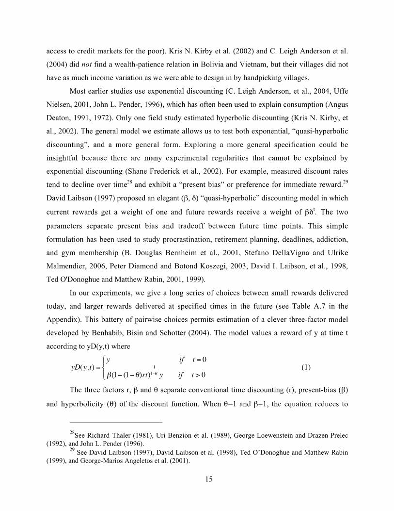
In our experiments, we give a long series of choices between small rewards delivered

today, and larger rewards delivered at specified times in the future (see Table A.7 in the

Appendix). This battery of pairwise choices permits estimation of a clever three-factor model

developed by Benhabib, Bisin and Schotter (2004). The model values a reward of y at time t

according to yD(y,t) where

€

yD(y,t) =y if t = 0

β(1− (1−θ)rt)11−θ y if t > 0

(1)

The three factors r, β and θ separate conventional time discounting (r), present-bias (β)

and hyperbolicity (θ) of the discount function. When θ=1 and β=1, the equation reduces to

28See Richard Thaler (1981), Uri Benzion et al. (1989), George Loewenstein and Drazen Prelec

(1992), and John L. Pender (1996).29 See David Laibson (1997), David Laibson et al. (1998), Ted O’Donoghue and Matthew Rabin

(1999), and George-Marios Angeletos et al. (2001).

16

exponential discounting. When θ=2 and β=1, it reduces to true hyperbolic discounting. When

θ=1 and β is free, it reduces to quasi-hyperbolic discounting. When θ>2 the function is “hyper-

hyperbolic”—the second derivative of the discount factor D(y,t) is even higher than for a

hyperbolic. The three-parameter form enables a way to compare three familiar models at once.

We used 15 combinations of y and t in the experiments, i.e. 30,000, 120,000 and 300,000

dong with the delays of one week, one month and three months, and 60,000 and 240,000 dong

with the delays of three days, two weeks and two months (see Table A.7 in the Appendix for all

combinations). The largest amount of y, 300,000 dong (about 19 dollars), is equivalent to 15

days of wage in the rural north.

For each (y,t) combination, we asked five questions, with x equal to 1/6, 1/3, 1/2, 2/3, and

5/6 of the value of y. Subjects were presented with a total of 75 choices between two options:

Option A: Receive x dong today.

Option B: Receive y dong in t days.

Subjects gave a switching point from preferring B to A in each series of five questions.

Before subject made choices, we suggested a trusted agent who would keep the money until

delayed delivery date to ensure subjects believed the money would be delivered. The selected

trusted persons were usually village heads or presidents of women’s associations. In some

villages, the trusted agents were also experimental subjects. Agreement letters of money delivery

were signed between the trusted agents and the first author. We cannot be certain that the money

amounts were delivered as promised. However, if villagers thought they could get the money

earlier, they would act very patiently, and they did not. After subjects completed all 75 questions,

we put 75 numbered balls in the bingo cage and drew one ball to determine which pairwise

choice would be paid. The option chosen for that question (i.e. A or B) determined how much

money was delivered, and when.

Table 8 shows the results from regressing estimates of Equation (1), allowing r (or ß) to

depend on demographic variables.30 For each subject, there are fifteen observations. We pooled

30 We consider middle points as indifferent points. We dropped data of 3 subjects, since they

totally randomized their choices. The estimates also exclude 315 observations which includedinconsistencies. Inconsistency means that a subject would accept a longer delay of a larger amount y,rather than taking x earlier, but would not wait for a shorter delay for the same y and x. (For example, ifan agent chooses 10,000 dong today over 60,000 dong with three days of delay, but is willing to wait 2months to receive 60,000 dong rather than receiving 10,000 dong today, their answers are inconsistent.).

17

data across all subjects and estimated Equation (1). In order to obtain robust variance estimates

with repeated observations on individual subjects, we specified that the observations are

independent across observations, but not within subjects. The estimated value of θ is around 5.3,

which is similar to Benhabib et al.’s (2004) estimates.

The largest effects are on discount rates r. Farmers, fishermen, and government officers

are more patient (lower r). Village mean income is negatively correlated with the discount rates.

This suggests in wealthier villages, people are more patient. On the other hand, relative income

within the village is positively correlated with the discount rates. W. Kip Viscusi and Michael J.

Moore (1989) assert that risky but high-paying jobs attract individuals with high discounting. It

may be that individuals with high time discounting did not miss opportunities to make profits

during the transition to the market economy.

Looking at the discount rate r and the present bias β together shows an interesting pattern

for ROSCA participants: ROSCA participants are more patient (lower r) and have less present

bias (higher β) than non-participants; but participants in bidding-ROSCAs are less patient

(higher r) and more present biased (lower β) than fixed-ROSCA participants.

The results suggest how experimental measurement can provide insights to institutional

design. Creating ROSCAs in which villagers will participate requires some knowledge of their

preferences and motives. Bidding ROSCAs may facilitate risk pooling, especially when people

face income uncertainty, because the order of receipts of money is not prearranged. But they also

seem to attract impatient people.

IV. Trust Game

We focus on one aspect of social preferences, trust, since it is considered a key element

of social capital (Partha Dasgupta, 2005, Steven Durlauf and Marcel Fafchamps, 2004, Stephen

Knack and Philip Keefer, 1997). We conducted the trust game of Joyce Berg, John Dickhaut and

Kevin McCabe (1995), a continuous relative of the binary trust game introduced earlier by Colin

C. Camerer and Keith Weigelt (1988).

We also conducted regressions for the south and north, separately. The estimation results or these separatesamples, and included the inconsistent observations, are shown in Tables A.8 and A.9 in the Appendix.Including the inconsistent ones rarely changes coefficient signs but adds noise and typically lowerssignificance.

18

In the trust game, one player, an “investor”, is endowed with capital she can keep or

invest. If she invests, there is a productive return—in our experiments, the investment triples. A

“trustee” then decides how much of the tripled investment to keep and how much to repay. There

is no contractual enforcement or reputation forces so self-interested trustees will keep all the

money; anticipating this, an investor who thinks trustees are self-interested (and is not altruistic)

will invest nothing. The trust game therefore captures a simple kind of investment with moral

hazard. Societies which manage to cultivate pure trust among strangers are probably more

economically efficient (e.g., Knack and Keefer (1997)) because pure trust is a substitute for

contractual enforcement, violence, and law.

There are many studies using trust games. An important difference between our study and

others is that we divided subjects into wealth groups, and observed whether behavior changes

depending on the wealth levels of the other party. Nava Ashraf, Iris Bohnet and Nikita Piankov

(2004), Michael R. Carter and Marco Castillo (2002), and Håkan J. Holm and Anders Dalienson

(2005) demonstrated how trusting behavior can be largely explained by altruism, because

trusting investors often do not expect to have much money repaid. We are interested in how

altruism is correlated with wealth and inequality. We use the Gini coefficient of the community

as a proxy for inequality.31

After an experimenter reads the instruction, the subjects solved a quiz. Illiterate subjects

and subjects who had difficulty understanding the game were helped by research assistants.32

After having solved the quiz, subjects went out of the room, one by one, and drew numbered

balls in a bingo cage. The subjects who drew odd numbers were assigned the roles of Player 1.

Subjects who drew an even number were assigned the role of Player 2.

31 The Gini coefficient is the relative area between a 45-degree line and a Lorenz curve. A Lorenz

curve graphs the cumulative proportion of income against cumulative population proportion, cumulatingfrom poorest to richest. Zero represents perfect equality, and 1 represents perfect inequality (one personowns everything). For comparison, the national Gini coefficient for the US was 0.45 in 2004, and theVietnam national figure was 0.36 in 1998 (CIA fact book

http://www.cia.gov/cia/publications/factbook/fields/2172.html). Worldwide, nationalGini’s range from around 0.25 (in Japan and western Europe) to 0.60 (mostly in Latin American andcentral Africa). So inequality within the Vietnamese villages (see Table 1) are relatively equal in incomecompared to many cross-country inequality in many countries.

32 Since the waiting time was long for the subjects who could not finish the quiz quickly, we hadenough time to explain the game to those slow subjects. Eventually, all subjects passed the quiz.

19

Player 1 was endowed with 20,000 dong, which was roughly equivalent to the daily wage

in rural north. Player 1 is then given a chance to send some money to Player 2 (in multiples of

2,000 dong). The experimenter triples the amount sent before it reaches Player 2. Player 2 is then

given a chance to send back as much money as he wants. We used the strategy method, asking

Player 1 how much they would send to Player 2 if Player 2 was in Group H, M and L,

respectively, so there is a within-subject comparison of how investor Player 1’s react to player

2’s in different income groups. In addition, we asked them to report how much they expect to get

back from Player 2 in Group H, M and L, respectively. We used the strategy method for Player 2

as well, asking how much they would send back to Player 1 for each of the 10 possible positive

investments. Subjects were helped by research assistants when making decisions. We made sure

subjects could not hear each other when making decisions. After filling out the record sheet, each

subject was given a questionnaire to fill in, and kept away from subjects who had not yet played

the game. Figure A.4 in the Appendix illustrates the experimental procedures.

The mean amounts sent by Player 1 were 10,324, 5,707 and 7,841 dong for student

subjects, and field experiments in the south and north, respectively. The fractions sent by Player

1’s in the south and north field sites, 28 percent and 40 percent respectively, are a little lower

than other studies conducted in Zimbabwe, South Africa, Honduras, Tanzania, Kenya,

Bangladesh, Peru, Uganda, and Paraguay (see Cardenas and Carpenter (2005)).33 However, the

fractions sent by Player 1’s in our student experiments, 52 percent, are compatible to other

studies in US, Russia, Tanzania and Sweden (Nava Ashraf, et al., 2004, Joyce Berg, et al., 1995,

Håkan J. Holm and Anders Danielson, 2005). Figure 2 graphs the amounts sent as cumulative

distribution functions (cdf’s), aggregating across north and south village sites. (Figure A.5 in the

Appendix contains student and village-specific cdf’s). In Figure 2, the x-axis point at which each

cdf intersects the horizontal line p=.5 is the median investment. Focusing attention on where the

different H, M and L cdf’s intersect the p=.5 line enables your eye to quickly see median

differences. The most striking difference is in the south where there is a substantial gap between

median investments to groups H, M and L; investors invest more with L groups than they do for

33 See Barr (1999, 2001), Ensminger (2000), Carter and Castillo (2002, 2003), Mosley and

Vershoor (2003), Johansson-Stenman et al. (2004), Holm and Danielson (2005), Karlan (forthcoming),and Schechter (2005).

20

H groups. This pattern is visible in all the villages in the south except S2 (Figure A.5).34 We

observe similar patterns in villages N1 and N2 in the north, i.e. Player 1 sent more to lower

income groups. However, we do not see significant difference in the amounts sent to different

income groups in village N3 and N4, the poorest villages (which historically are also the most

communized).

Keep in mind investments are not necessarily expectations of reciprocal repayment.

Ashraf, Bohnet and Piankov (2004) showed trusting investments might also just reflect altruistic

giving to other players, because the investment-tripling multiplier means investing a small

amount creates a much larger amount the second player could keep. The expected return ratio is

calculated as the expected amount of money back divided by the amount of money sent (tripled

amount). Both in the South and North, Player 1 tend to expect higher returns from group H and

lower returns from group L. A natural interpretation of the tendency in the south therefore is the

subjects give more to the poor (the L group), and less to the rich (the H group) because they are

redistributing wealth, not because they expect repayment. The fact this pattern is less evident in

the North suggests an effect of political institutions crowding out private transfer—in the North,

communist redistribution equalizes resources, but in the South, villagers redistribute income

from rich to poor on their own.

Table 9 shows the results of linear regressions on the amount sent by Player 1 for field

experiments. We first conducted regressions for the south and north separately, and then ran

regressions, pooling data from both regions.35

Player 1’s who engage in trading activities also sent significantly higher amount of

money to Player 2 in both regions when we conduct regressions separately. However, the

estimated coefficients are not significant when we pool the data from both regions. Player 1 who

engages in family businesses sent less money to Player 2, especially in the north. Recall

individuals with household business are much wealthier in the north. In all of the north villages,

34 However, notice from Table 1 that the Gini coefficient of village S2 is small, 0.19, and the

mean income of groups M and L are close. It may have been difficult for the subjects to recognize anydifference in wealth between groups M and L.

35 Since there are repeated observations on individual subjects, we specified that the observationsare not independent within subjects. We also ran regressions with the survey responses to the GSSquestions on trust, fairness and helpfulness, but they were not significant.

21

there are only five subjects who receive remittance from their oversea relatives. They send

significantly more money to Player 2, an indication of private communal sharing of remittances.

The estimated coefficients of mean income of the community are weakly significant in

both regions but are positive in the south, and negative in the north. The negative correlation

between the income levels of the community and the amount sent by Player 1 in the north may

be due to collectivism. In poor villages in the north, experimental subjects are predominantly

farmers who had worked on collective farms for many years. The Gini coefficient is negative and

significant in the south, and is also significant for the pooled data estimations. Our findings

support Knack and Keefer’s (1997) conclusion that trust is positively correlated with equality. In

the south, Player 1 sends significantly larger amount of money to Player 2 in Groups M and L.

This redistribution trend within villages is much weaker in the north, another statistical

indication of a crowding-out effect of political institutions on private transfers.

Figure 4 illustrates the amount of money sent back by Player 2 in each session.

Generally, trust pays off among student subjects and non-student subjects in the north in most

villages and across all income groups (because the amount returned is greater than the amount

sent). By contrast, in the south, Player 2 sent back more than Player 1 sent them only for group L

members in Villages S1 and S2, the wealthiest villages. It may be that Group L in these wealthy

villages felt they needed to prove they are not underprivileged.

Table 10 presents the results of linear regressions on the proportion of money sent back

by Player 2 in the field experiments. Coefficients of relative income are positive in all

regressions. This implies wealthy individuals are more inclined to reciprocate. The poor in

wealthy communities are also significantly more reciprocal in the south. Older and male

subjects and those who engage in trading activities also repay more. The total number of

government officers in the experiment has positive impacts on the proportion of money sent back

when we ran regressions separately for each region. This implies the presence of government

officers, who are often communist party members, enhances social norms. Also, the dummy

variable for South is negative and significant, confirming positive effects of stronger

communism on reciprocity in the North. Contrary to our expectation, ROSCA participants in the

north reciprocate less.

Table 11 shows the relation between risk parameters (α, σ, and λ), time discounting, and

trust. Time discounting is measured as the mean discount factor, D(y,t), across 15 combinations

22

of y and t. Vital Anderhub et al. (2001) find negative relations between risk aversion and time

discounting. In our study, we do not find a significant correlation between risk parameters and

time discounting. As Anderhub et al. point out, subjects’ risk aversion is sensitive to the

experimental procedure. The fact we do not find significant relations between risk and time

discounting in our study suggests our subjects felt secure about the delayed money delivery.

Ashraf, Bohnet, and Piankov (2004) and Catherine C. Eckel and Rick K. Wilson (2004)

do not find significant relations between risk and trust, while Laura Schechter (2005) finds

positive relations between risk and trust. In our experiments, risk aversion is not correlated with

trust but we find positive relations between trust and probability weighting. Player 1 with

inflected probability weights send more money to Player 2. This is consistent with the idea that

they treat a trusting investment as a gamble and overweight the chance of winning.

We also find a weak positive relation between the curvature of value function and the

curvature of the weighting function, as well as loss aversion. This implies subjects who are less

risk-averse exhibit more linear weighting and are less loss-averse.

V. Conclusion

We conducted abstract experiments in Vietnam to investigate whether village wealth,

political history, the choice of occupation, and other surveyed variables are correlated with

fundamental preferences. Our study is unique in its ability to link many different experimental

measures of preferences to a wide range of previously-surveyed demographic variables. These

results are exploratory and the experimental measures are not perfect. Further, as noted in the

introduction, in a cross-sectional study it’s difficult to conclude very much about the direction of

causality between preferences and economic circumstances because the study was not designed

to do so. Nonetheless, we can identify certain patterns that could be explored in further work and

investigated in other field sites.

South/North: People in the north had worked on collective farms for many years, and

the government had provided them with food for subsistence. As a result, one can speculate that

villagers in the south are more loss averse (higher λ) than those in the north. At the same time,

there is no evident difference in time preference parameters in the two regions.

23

It seems people in the south are more altruistic toward the poor: In trust games villagers

in the south invest more in the poor L group and less in the wealthier H group (Figure 2), but not

expect to be repaid more by the L group (Figure 3). This pattern is consistent with the idea that

private norms of redistribution from rich to poor are active in the South but are crowded out in

the North possibly by communist public institutions, although we observe a strong overall

positive effect of communism on reciprocity across all income groups.36

Village income: Previous experiments show inconsistent results on whether wealth is

positively or negatively correlated with risk-aversion. Our results show people in poorer villages

are not necessarily more risk-averse, but they are more loss-averse (Table 7). This difference is a

reminder that in EU, the only source of risk-aversion is concavity of utility over monetary

outcomes. Prospect theory suggests three dimensions of risk-aversion, and only loss-aversion is

correlated with village income. Mean village income is also correlated with lower discount rates

(r) and less present bias (higher β). This data suggests economic development could influence

preferences; the wealthier the villages become, the less loss averse and more patient their

villagers are.

ROSCAs: ROSCA participation is correlated with risk and time preferences in two

interesting ways. Participants in bidding ROSCAs are more risk-averse (higher σ). This result is

consistent with discussions in the empirical literature considering bidding ROSCAs as insurance

devices when people face income uncertainty (Charles W. Calomiris and Indora Rajaraman,

1998, Stefan Klonner, 2003). Furthermore, those who participate in bidding ROSCAs, compared

to fixed ROSCAs, are more impatient.

Occupation: There are some interesting scattered effects of occupation. While these

results do not cohere into patterns across parameters and analyses, they are worth noting as a

guide to future research, and in aggregating results across many studies. Furthermore,

occupations and preference are important for development if shepherding the poor into some

occupations are likely to inculcate preferences which are good for later growth (such as patience

and trust). Table 7 shows that fishermen are less risk-averse, probably a selection effect because

fishing is inherently risky (but also profitable). Government officers are less loss-averse, perhaps

36 Terry A. Rambo (1973) reports that Northern villages have traditionally acted as autonomous

political units. It is possible that stronger social norms had already developed in the north before thecommunist regime.

24

because their political ties and power cushion them in downturns. Tables 9-10 show villagers

engage in trade— usually modest roadside businesses— are both more trusting and more

trustworthy. This result is consistent with finding of Joseph Henrich et al (2005), based on a

study across 15 small-scale societies, that market integration is correlated with fair sharing in

ultimatum games.

By using richer instruments, we were able to separate different aspects of risk aversion

and time preferences. While our broad experiment was not designed to study the efficacy of

specialized policy instruments, the results show some potential policy implications which differ

from those of other studies which use simpler preference models. For example, the results

indicate the people living in poor villages are not necessarily afraid of uncertainty, in the sense of

income variation; instead, they are averse to loss. On the other hand, villagers in the north who

had worked on collective farms and received food from the government on a regular basis are

less averse to loss. To the extent that preferences are shaped by circumstances and traditions, the

first pattern implies that increasing village wealth will reduce aversion to loss (and alleviate the

need for policies that limit income fluctuation).

By decomposing time preferences into conventional discount rates and present bias, we

found the mean village income was correlated with lower discount rates and with less present

bias. People who are present-biased, and are sophisticated about their bias, realize the need for

external commitment. Thus, these results suggest that policy could usefully focus not on

increasing patience or subsidizing savings, per se, but on providing more present-biased villagers

with external commitment (as in Ashraf, Karlan and Yin (forthcoming)).

The results also show how preference measurement can provide suggestions for

institutional design. The design of ROSCAs requires some knowledge of the preferences and

motives of potential participants. Bidding ROSCAs may facilitate risk pooling, especially when

people face income uncertainty, because the order of receipts of money is not prearranged. But

bidding ROSCAs also seem to attract impatient people.

As noted throughout, these results are exploratory and need to be replicated in these sites,

and compared with results in other sites (as in Cardenas and Carpenter’s (2005) important meta-

analysis). An advantage of the low mobility in the Vietnamese villages, and government control,

is that in principle we can revisit these villages in the future, conduct the same experiments with

25

the same people (and add other measures), to create panel experimental data which are better

suited to establishing selection effects than this cross-sectional study can.

Finally, we hope one contribution of our study is to show some advantages of expanding

measurements of risk and time preferences beyond expected utility and exponential discounting,

replacing those simple approximations with prospect theory and the Benhabib et al. three-

parameter discounting model. In a poor, highly literate country, our subjects made

comprehensible choices in a large battery of tasks while highly motivated to earn money. While

these experiments take time, but subjects in these sites are often eager to participate and their

opportunity cost of participating is low. As a result, and as in most anthropology experiments

(Joseph Henrich, et al., 2005), these subjects will sit patiently and answer questions studiously

while many dimensions of their economic life are measured, the experimental facts that are

produced, and the interesting correlations that result, suggest that these instruments could be

used in many other sites as well.

26

References

Anderhub, Vital; Guth, Werner; Gneezy, Uri and Sonsino, Doron. "On the Interaction of

Risk and Time Preferences - an Experimental Study." German Economic Review, 2001, 2(3), pp.

239-53.

Anderson, C. Leigh; Dietz, Maya; Gordon, Andrew and Klawitter, Marieka. "Discount

Rates in Vietnam." Economic Development and Cultural Change, 2004, 52(4), pp. 873-88.

Anderson, Siwan and Baland, Jean-Marie. "The Economics of Roscas and Intrahousehold

Resource Allocation." Quarterly Journal of Economics, 2002, 117(3), pp. 963-95.

Angeletos, George-Marios; Laibson, David; Repetto, Andrea; Tobacman, Jeremy and

Weinberg, Stephen. "The Hyperbolic Consumption Model: Calibration, Simulation, and

Empirical Evaluation." Journal of Economic Perspectives, 2001, 15(3), pp. 47-68.

Ashraf, Nava; Bohnet, Iris and Piankov, Nikita. "Is Trust a Bad Investment?" Harvard

University Working Paper, 2004.

Ashraf, Nava; Karlan, Dean S. and Yin, Wesley. "Tying Odysseus to the Mast: Evidence from

a Commitment Savings Product in the Philippines." Quarterly Journal of Economics,

forthcoming.

Bardhan, Pranab and Udry, Christopher. Development Microeconomics. Oxford: Oxford

University Press, 1999.

Barr, Abagail. "Familiarity and Trust: An Experimental Investigation," Oxford University

Center for the Study of African Economies Working Paper, 1999.

Barr, Abigail. "Trust and Expected Trustworthiness: An Experimental Investigation,"

University of Oxford Centre of the Study of African Economics Working Paper, 2001.

Becker, Gary S. and Mulligan, Casey B. "The Endogenous Determination of Time

Preference." Quarterly Journal of Economics, 1997, 112(3), pp. 729-58.

Benhabib, Jess; Bisin, Alberto and Schotter, Andrew. "Hyperbolic Discounting: An

Experimental Analysis," New York University Department of Economics Working Paper, 2004.

Benzion, Uri; Rapoport, Amnon and Yagil, Joseph. "Discount Rates Inferred from Decisions

- an Experimental-Study." Management Science, 1989, 35(3), pp. 270-84.

Berg, Joyce; Dickhaut, John and McCabe, Kevin. "Trust, Reciprocity and Social History."

Games and Economic Behavior, 1995, 10, pp. 122-42.

27

Bernheim, B. Douglas; Skinner, Jonathan and Weinberg, Stephen. "What Accounts for the

Variation in Retirement Wealth among U.S. Households?" American Economic Review, 2001,

91(4), pp. 832-57.

Binswanger, Hans P. "Attitudes toward Risk: Experimental Measurement in Rural India."

American Journal of Agricultural Economics, 1980, 62, pp. 395-407.

____. "Attitudes toward Risk: Theoretical Implications of an Experiment in Rural India."

Economic Journal, 1981, 91(364), pp. 867-90.

Bouman, F.J.A. "Rotating and Accumulating Savings and Credit Associations: A Development

Perspective." World Development, 1995, 23(3), pp. 371-84.

Bowles, Samuel. "Endogenous Preferences: The Cultural Consequences of Markets and Other

Economic Institutions." Journal of Economic Literature, 1998, 36(1), pp. 75-111.

Braverman, Avishay and Stiglitz, Joseph E. "Sharecropping and the Interlinking of Agrarian

Markets." American Economic Review, 1982, 72(4), pp. 695-715.

Calomiris, Charles W. and Rajaraman, Indora. "The Role of Rsocas: Lumpy Durables or

Event Insurance?" Journal of Development Economics, 1998, 56, pp. 207-16.

Camerer, Colin F. "Prospect Theory in the Wild," D. Kahneman and A. Tversky, Choices,

Values and Frames. Cambridge: Cambridge University Press, 2000,

Camerer, Colin F. and Weigelt, Keith. "Experimental Tests of a Sequential Equilibrium

Reputation Model." Econometrica, 1988, 56(1), pp. 1-36.

Cardenas, Juan-Camilo and Carpenter, Jeffrey. "Experiments on Equipment: Lessons from

Labs in the Field around the World," Universidad de los Andes Facultad de Economia Working

Paper, 2005.

Carter, Michael R. and Castillo, Marco. "The Economic Impacts of Altruism, Trust and

Reciprocity: An Experimental Approach to Social Capital," University of Wisconsin-Madison

Agricultural & Applied Economics Staff Paper, 2002.

____. "An Experimental Approach to Social Capital in South Africa," University of Wisconsin-

Madison Agricultural & Applied Economics Staff Paper, 2003.

Dasgupta, Partha. "The Economics of Social Capital," University of Cambridge Working

Paper, 2005.

Deaton, Angus. "Saving and Liquidity Constraints." Econometrica, 1991, 59(5), pp. 1221-48.

28

____. "Wealth Effects on Consumption in a Modified Life-Cycle Model." Review of Economic

Studies, 1972, 39(4), pp. 443-53.

DellaVigna, Stefano and Malmendier, Ulrike. "Paying Not to Go to the Gym." American

Economic Review, 2006, forthcoming.

Diamond, Peter and Koszegi, Botond. "Quasi-Hyperbolic Discounting and Retirement."

Journal of Public Economics, 2003, 87, pp. 1839-72.

Duflo, Esther. "Field Experiments in Development Economics," World Congress. London,

2005.

Durlauf, Steven and Fafchamps, Marcel. "Social Capital," NBER Working Paper, 2004.

Eckel, Catherine C. and Wilson, Rick K. "Is Trust a Risky Decision?" Journal of Economic

Behavior and Organization, 2004, 55(4), pp. 447-65.

Eggert, Håkan and Martinsson, Peter. "Are Commercial Fishers Risk Lovers?" Göteborg

University Working Paper, 2003.

Ensminger, Jean. "Experimental Economics in the Bush: Why Institutions Matter," C. Menard,

Institutions and Organizations. London: Edward Elgar, 2000,

Fafchamps, Marcel and Pender, John. "Precautionary Saving, Credit Constraints, and

Irreversible Investment: Theory and Evidence from Semiarid India." Journal of Business and

Economic Statistics, 1997, 15(2), pp. 180-94.

Frederick, Shane; Loewenstein, George and O'Donoghue, Ted. "Time Discounting and Time

Preference: A Critical Review." Journal of Economic Literature, 2002, 40(2), pp. 351-401.

Gugerty, Mary Kay. "You Can’t Save Alone: Commitment in Rotating Savings and Credit

Associations in Kenya," University of Washington Working Paper, 2005.

Hansen, James; Marx, Sabine and Weber, Elke. "Expectations and Forecasts in Farmer

Decision Making: The Argentine Pampas and South Florida," New York: International Research

Institute for Climate Prediction (IRI), 2004.

Harbaugh, William T.; Krause, Kate and Liday, Steve. "Children's Bargaining Behavior:

Differences by Age, Gender, and Height," University of Oregon Working Paper, 2000.

Harrison, Glenn W.; Lau, Morten I. and Williams, Melonie B. "Estimating Individual

Discount Rates in Denmark: A Field Experiment." American Economic Review, 2002, 92(5), pp.

1606-17.

29

Haughton, Jonathan and Vijverberg, Wim P.M. "Household Enterprises in Vietnam:

Survival, Growth, and Living Standards," World Bank Working Paper, 2002.

Hausman, Jerry. "Individual Discount Rates and the Purchase and Utilization of Energy-Using

Durables." Bell Journal of Economics, 1979, 10(1), pp. 33-54.

Henrich, Joseph; Boyd, Robert; Bowles, Samuel; Camerer, Colin; Fehr, Ernst; Gintis,

Herbert; McElreath, Richard; Alvard, Michael; Barr, Abigail; Ensminger, Jean, et al.

"‘Economic Man’ in Cross-Cultural Perspective: Ethnography and Experiments from 15 Small-

Scale Societies." Behavioral and Brain Sciences, 2005, 28, pp. 795-855.

Henrich, Joseph and McElreath, Richard. "Are Peasants Risk-Averse Desicion Makers?"

Current Anthropology, 2002, 43(1), pp. 172-81.

Ho, Tech H.; Lim, Noah and Camerer, Colin. "'Modeling the Psychology of Consumer and

Firm Behavior with Behavioral Economics." Journal of Marketing Research, 2006, 43(3).

Holm, Håkan J. and Danielson, Anders. "Tropic Trust Versus Nordic Trust: Experimental

Evidence from Tanzania and Sweden." Economic Journal, 2005, 115(503), pp. 505-32.

Holt, Charles A. and Laury, Susan K. "Risk Aversion and Incentive Effects." American

Economic Review, 2002, 92(5), pp. 1644-55.

Humphrey, Steven J. and Verschoor, Arjan. "The Probability Weighting Function:

Experimental Evidence from Uganda, India and Ethiopia." Economics Letters, 2004, 84(3), pp.

419-25.

Johansson-Stenman, Olof; Mahmud, Minhaj and Martinsson, Peter. "Trust, Trust Games

and Stated Trust: Evidence from Rural Bangladesh," Göteborg University Department of

Economics Working Paper, 2004.

Kahneman, Daniel and Tversky, Amos. "Prospect Theory - Analysis of Decision under Risk."

Econometrica, 1979, 47(2), pp. 263-91.

Kanbur, Ravi and Squire, Lyn. "The Evolution of Thinking About Poverty," G. M. Meier and

J. E. Stiglitz, Frontiers of Development Economics. Oxford: Oxford University Press, 2001,

Karlan, Dean S. "Using Experimental Economics to Measure Social Capital and Predict

Financial Decisions." American Economic Review, forthcoming.

Kirby, Kris N.; Godoy, Ricardo; Reyes-Garcia, Victoria; Byron, Elizabeth; Apaza, Lilian;

Leonard, William; Perez, Eddy; Vadez, Vincent and Wilkie, David. "Correlates of Delay-

30

Discount Dates: Evidence from Tsimane' Amerindians of the Bolivian Rain Forest." Journal of

Economic Psychology, 2002, 23, pp. 291-316.

Klonner, Stefan. "Rotating Savings and Credit Associations When Participants Are Risk

Averse." International Economic Review, 2003, 44(3), pp. 979-1005.

Knack, Stephen and Keefer, Philip. "Does Social Capital Have an Economic Payoff? A Cross-

Country Investigation." Quarterly Journal of Economics, 1997, 112(4), pp. 1251-88.

Laibson, David. "Golden Eggs and Hyperbolic Discounting." Quarterly Journal of Economics,

1997, 112(2), pp. 443-77.

Laibson, David I.; Repetto, Andrea and Tobacman, Jeremy. "Self-Control and Saving for

Retirement." Brookings Papers on Economic Activity, 1998, (1), pp. 91-196.

Lawrance, Emily C. "Poverty and the Rate of Time Preference: Evidence from Panel Data."

Journal of Political Economy, 1991, 99(1), pp. 54-77.

Loewenstein, George and Prelec, Drazen. "Anomalies in Intertemporal Choice: Evidence and

an Interpretation." Quarterly Journal of Economics, 1992, 107(2), pp. 573-97.

Mosley, Paul and Verschoor, Arjan. "The Development of Trust and Social Capital in Rural

Uganda: An Experimental Approach," University of Sheffield Working Paper, 2003.

Mosley, Paul and Verschoor, Arjan. "Risk Attitudes and the 'Vicious Circle of Poverty'."

European Journal of Development Research, 2005, 17(1), pp. 59-88.

Nielsen, Uffe. "Poverty and Attitudes Towards Time and Risk - Experimental Evidence from

Madagascar," Royal Veterinary and Agricultural University of Denmark Department of

Economics and Natural Resources. 2001.

O'Donoghue, Ted and Rabin, Matthew. "Choice and Procrastination." Quarterly Journal of

Economics, 2001, 116(1), pp. 121-60.

____. "Doing It Now or Later." American Economic Review, 1999, 89(1), pp. 103-24.

Pender, John L. "Discount Rates and Credit Markets: Theory and Evidence from Rural India."

Journal of Development Economics, 1996, 50, pp. 257-96.

Petry, Nancy M.; Armentano, Christoff, Kalina; Kuoch, Theanvy; Norinth, Thonguan and

Smith, Lien. "Gambling Participation and Problems among South East Asian Refrees to the

United States." American Psychiatric Association, 2003, 54(8), pp. 1142-48.

Pingali, Prabhu and Xuan, Vo-Tong. "Vietnam: Decollectization and Rice Productivity

Growth." Economic Development and Cultural Change, 1992, 40(4), pp. 697-718.

31

Prelec, Drazen. "The Probability Weighting Function." Econometrica, 1998, 66(3), pp. 497-527.

Rambo, A. Terry. Comparison of Peasant Social Systems of Northern and Southern Viet-Nam:

A Study of Ecological Adaptation, Social Succession, and Cultural Evolution. Center for

Vietnamese Studies, Southern Illinois University, 1973.

Rilling, James K.; Gutman, David A.; Zeh, Thorsten R.; Pagnoni, Gluseppe; Berns,

Gregory S. and Kilts, Clinton D. "A Neural Basis for Social Cooperation." Neuron, 2002,

35(2), pp. 395-405.

Rosenzweig, Mark R. and Binswanger, Hans P. "Wealth, Weather Risk and the Composition

and Profitability of Agricultural Investments." Economic Journa l, 1993, 103(416), pp. 56-78.

Schechter, Laura. "Traditional Trust Measurement and the Risk Confound: An Experiment in

Rural Paraguay." Journal of Economic Behavior and Organization, 2005, forthcoming.

Thaler, Richard. "Some Empirical-Evidence on Dynamic Inconsistency." Economics Letters,

1981, 8(3), pp. 201-07.

Tversky, Amos and Kahneman, Daniel. "Advances in Prospect-Theory - Cumulative

Representation of Uncertainty." Journal of Risk and Uncertainty, 1992, 5(4), pp. 297-323.

van de Walle, Dominique and Cratty, Dorothyjean. "Is the Emerging Non-Farm Market

Economy the Route out of Poverty in Vietnam?" The economics of transition, 2004, 12(2), pp.

237-74.

Viscusi, W. Kip and Moore, Michael J. "Rates of Time Preference and Valuation of the

Duration of Life." Journal of Public Economics, 1989, 38(3), pp. 297-317.

Wik, Mette and Holden, Stein. "Experimental Studies of Peasant's Attitutes toward Risk in

Northern Zambia," Agricultural University of Norway Department of Economics and Social

Sciences Working Paper, 1998.

Wu, George and Gonzalez, Richard. "Curvature of the Probability Weighting Function."

Management Science, 1996, 42(12), pp. 1976-690.

Xuan, Vo-Tong. "Rice Production, Agricultural Research, and the Environment," B. J. T.

Kerkvliet and D. J. Porter, Vietnam's Rural Transformation. Boulder: Westview Press, 1995,

Yesuf, Mahmud. "Risk, Time and Land Management under Market Imperfections: Applications

to Ethiopia," Göteborg University Department of Economics Working Paper, 2004.

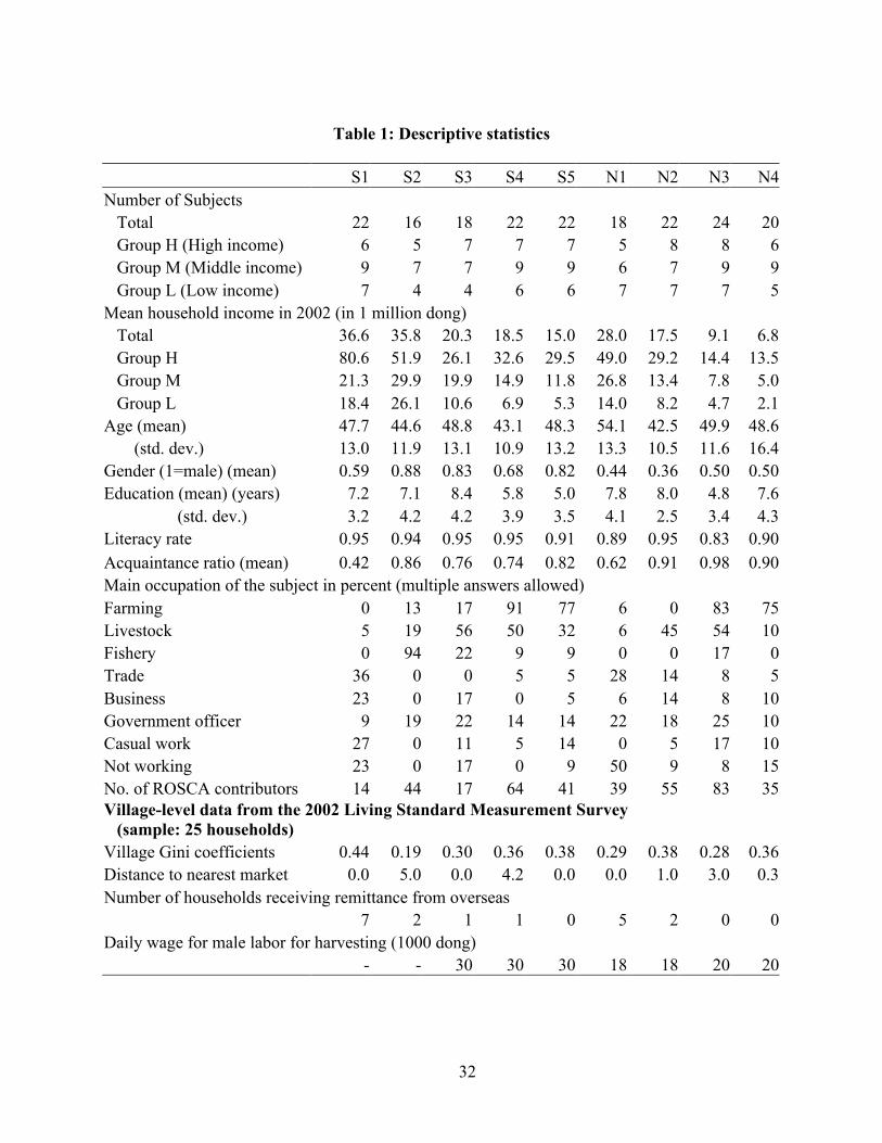
32

Table 1: Descriptive statistics

S1 S2 S3 S4 S5 N1 N2 N3 N4Number of Subjects Total 22 16 18 22 22 18 22 24 20 Group H (High income) 6 5 7 7 7 5 8 8 6 Group M (Middle income) 9 7 7 9 9 6 7 9 9 Group L (Low income) 7 4 4 6 6 7 7 7 5Mean household income in 2002 (in 1 million dong) Total 36.6 35.8 20.3 18.5 15.0 28.0 17.5 9.1 6.8 Group H 80.6 51.9 26.1 32.6 29.5 49.0 29.2 14.4 13.5 Group M 21.3 29.9 19.9 14.9 11.8 26.8 13.4 7.8 5.0 Group L 18.4 26.1 10.6 6.9 5.3 14.0 8.2 4.7 2.1Age (mean) 47.7 44.6 48.8 43.1 48.3 54.1 42.5 49.9 48.6 (std. dev.) 13.0 11.9 13.1 10.9 13.2 13.3 10.5 11.6 16.4Gender (1=male) (mean) 0.59 0.88 0.83 0.68 0.82 0.44 0.36 0.50 0.50Education (mean) (years) 7.2 7.1 8.4 5.8 5.0 7.8 8.0 4.8 7.6 (std. dev.) 3.2 4.2 4.2 3.9 3.5 4.1 2.5 3.4 4.3Literacy rate 0.95 0.94 0.95 0.95 0.91 0.89 0.95 0.83 0.90Acquaintance ratio (mean) 0.42 0.86 0.76 0.74 0.82 0.62 0.91 0.98 0.90Main occupation of the subject in percent (multiple answers allowed)Farming 0 13 17 91 77 6 0 83 75Livestock 5 19 56 50 32 6 45 54 10Fishery 0 94 22 9 9 0 0 17 0Trade 36 0 0 5 5 28 14 8 5Business 23 0 17 0 5 6 14 8 10Government officer 9 19 22 14 14 22 18 25 10Casual work 27 0 11 5 14 0 5 17 10Not working 23 0 17 0 9 50 9 8 15No. of ROSCA contributors 14 44 17 64 41 39 55 83 35Village-level data from the 2002 Living Standard Measurement Survey (sample: 25 households)Village Gini coefficients 0.44 0.19 0.30 0.36 0.38 0.29 0.38 0.28 0.36Distance to nearest market 0.0 5.0 0.0 4.2 0.0 0.0 1.0 3.0 0.3Number of households receiving remittance from overseas

7 2 1 1 0 5 2 0 0Daily wage for male labor for harvesting (1000 dong)

- - 30 30 30 18 18 20 20

33

Table 2: Variable definitions

Variable name DescriptionAge Age of the subjectGender Gender of the subject, 1=maleEducation Number of years the subject attended school

Acquaintance ratioNumber of other subjects the subject knows by name divided by thetotal numberof subjects in the session

Farm/livestock Subject's main occupation is farming or raising livestockFishery Subject's main occupation is fishingTrade Subject's main occupation is tradingBusiness The subject is engaged in household businessGovernment officer The subject works for a local government

Relative income Subject's household income divided by the mean household income ofthe village

Mean village income Mean household income of the village (million dong)Gini coefficient Gini coefficient of the income among 25 households surveyed in 2002Distance to market Distance to the nearest local market (km)(Table 7)ROSCA 1=the member of ROSCA, 0=otherwiseROSCA*Bidding 1=the member of Bidding ROSCA, 0=otherwise(Table 8)Trusted agent The subject is a trusted agent of delayed delivery of money

Log (savings) Logged savings. Savings is measured as the total value of savings incash, gold and savings accounts.

Exp/income ratio Household expenditure divided by household income per year(Table 9)Oversea remittance Whether the subject is receiving remittance from overseas, 1=YesNumber of officers Number of local government officers in the sessionReceiver M 1=Player 2 is in Group MReceiver L 1=Player 2 is in Group L(Table 10)Group M 1=Player 2 is in Group M

M*Mean village income The cross effect of Mean village income and Player 2 being in GroupM

Group L 1=Player 2 is in Group LL*Mean village income The cross effect of Mean village income and Player 2 being in Group L

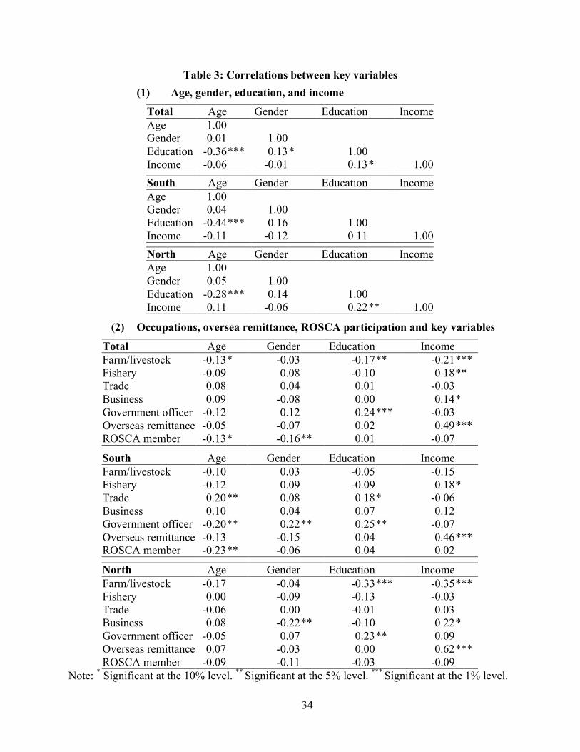
34

Table 3: Correlations between key variables(1) Age, gender, education, and income

Total Age Gender Education IncomeAge 1.00Gender 0.01 1.00Education -0.36*** 0.13* 1.00Income -0.06 -0.01 0.13* 1.00South Age Gender Education IncomeAge 1.00Gender 0.04 1.00Education -0.44*** 0.16 1.00Income -0.11 -0.12 0.11 1.00North Age Gender Education IncomeAge 1.00Gender 0.05 1.00Education -0.28*** 0.14 1.00Income 0.11 -0.06 0.22** 1.00

(2) Occupations, oversea remittance, ROSCA participation and key variables

Total Age Gender Education IncomeFarm/livestock -0.13* -0.03 -0.17** -0.21***Fishery -0.09 0.08 -0.10 0.18**Trade 0.08 0.04 0.01 -0.03Business 0.09 -0.08 0.00 0.14*Government officer -0.12 0.12 0.24*** -0.03Overseas remittance -0.05 -0.07 0.02 0.49***ROSCA member -0.13* -0.16** 0.01 -0.07

South Age Gender Education IncomeFarm/livestock -0.10 0.03 -0.05 -0.15Fishery -0.12 0.09 -0.09 0.18*Trade 0.20** 0.08 0.18* -0.06Business 0.10 0.04 0.07 0.12Government officer -0.20** 0.22** 0.25** -0.07Overseas remittance -0.13 -0.15 0.04 0.46***ROSCA member -0.23** -0.06 0.04 0.02

North Age Gender Education IncomeFarm/livestock -0.17 -0.04 -0.33*** -0.35***Fishery 0.00 -0.09 -0.13 -0.03Trade -0.06 0.00 -0.01 0.03Business 0.08 -0.22** -0.10 0.22*Government officer -0.05 0.07 0.23** 0.09Overseas remittance 0.07 -0.03 0.00 0.62***ROSCA member -0.09 -0.11 -0.03 -0.09

Note: * Significant at the 10% level. ** Significant at the 5% level. *** Significant at the 1% level.

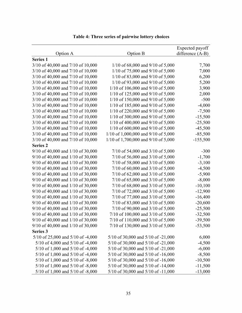
35

Table 4: Three series of pairwise lottery choices

Option A Option BExpected payoffdifference (A-B)

Series 13/10 of 40,000 and 7/10 of 10,000 1/10 of 68,000 and 9/10 of 5,000 7,7003/10 of 40,000 and 7/10 of 10,000 1/10 of 75,000 and 9/10 of 5,000 7,0003/10 of 40,000 and 7/10 of 10,000 1/10 of 83,000 and 9/10 of 5,000 6,2003/10 of 40,000 and 7/10 of 10,000 1/10 of 93,000 and 9/10 of 5,000 5,2003/10 of 40,000 and 7/10 of 10,000 1/10 of 106,000 and 9/10 of 5,000 3,9003/10 of 40,000 and 7/10 of 10,000 1/10 of 125,000 and 9/10 of 5,000 2,0003/10 of 40,000 and 7/10 of 10,000 1/10 of 150,000 and 9/10 of 5,000 -5003/10 of 40,000 and 7/10 of 10,000 1/10 of 185,000 and 9/10 of 5,000 -4,0003/10 of 40,000 and 7/10 of 10,000 1/10 of 220,000 and 9/10 of 5,000 -7,5003/10 of 40,000 and 7/10 of 10,000 1/10 of 300,000 and 9/10 of 5,000 -15,5003/10 of 40,000 and 7/10 of 10,000 1/10 of 400,000 and 9/10 of 5,000 -25,5003/10 of 40,000 and 7/10 of 10,000 1/10 of 600,000 and 9/10 of 5,000 -45,5003/10 of 40,000 and 7/10 of 10,000 1/10 of 1,000,000 and 9/10 of 5,000 -85,5003/10 of 40,000 and 7/10 of 10,000 1/10 of 1,700,000 and 9/10 of 5,000 -155,500Series 29/10 of 40,000 and 1/10 of 30,000 7/10 of 54,000 and 3/10 of 5,000 -3009/10 of 40,000 and 1/10 of 30,000 7/10 of 56,000 and 3/10 of 5,000 -1,7009/10 of 40,000 and 1/10 of 30,000 7/10 of 58,000 and 3/10 of 5,000 -3,1009/10 of 40,000 and 1/10 of 30,000 7/10 of 60,000 and 3/10 of 5,000 -4,5009/10 of 40,000 and 1/10 of 30,000 7/10 of 62,000 and 3/10 of 5,000 -5,9009/10 of 40,000 and 1/10 of 30,000 7/10 of 65,000 and 3/10 of 5,000 -8,0009/10 of 40,000 and 1/10 of 30,000 7/10 of 68,000 and 3/10 of 5,000 -10,1009/10 of 40,000 and 1/10 of 30,000 7/10 of 72,000 and 3/10 of 5,000 -12,9009/10 of 40,000 and 1/10 of 30,000 7/10 of 77,000 and 3/10 of 5,000 -16,4009/10 of 40,000 and 1/10 of 30,000 7/10 of 83,000 and 3/10 of 5,000 -20,6009/10 of 40,000 and 1/10 of 30,000 7/10 of 90,000 and 3/10 of 5,000 -25,5009/10 of 40,000 and 1/10 of 30,000 7/10 of 100,000 and 3/10 of 5,000 -32,5009/10 of 40,000 and 1/10 of 30,000 7/10 of 110,000 and 3/10 of 5,000 -39,5009/10 of 40,000 and 1/10 of 30,000 7/10 of 130,000 and 3/10 of 5,000 -53,500Series 35/10 of 25,000 and 5/10 of -4,000 5/10 of 30,000 and 5/10 of -21,000 6,0005/10 of 4,000 and 5/10 of -4,000 5/10 of 30,000 and 5/10 of -21,000 -4,5005/10 of 1,000 and 5/10 of -4,000 5/10 of 30,000 and 5/10 of -21,000 -6,0005/10 of 1,000 and 5/10 of -4,000 5/10 of 30,000 and 5/10 of -16,000 -8,5005/10 of 1,000 and 5/10 of -8,000 5/10 of 30,000 and 5/10 of -16,000 -10,5005/10 of 1,000 and 5/10 of -8,000 5/10 of 30,000 and 5/10 of -14,000 -11,5005/10 of 1,000 and 5/10 of -8,000 5/10 of 30,000 and 5/10 of -11,000 -13,000

36

Table 5: Switching point (question at which preference switches from option A to option B)and approximations of σ, α and λ under Prospect Theory

Series 1 (Question 1-14) Series 2 (Question 15-28).4 .5 .6 .7 .8 .9 1 .4 .5 .6 .7 .8 .9 1

.2 9 10 11 12 13 14 never .2 never 14 13 12 11 10 9

.3 8 9 10 11 12 13 14 .3 14 13 12 11 10 9 8

.4 7 8 9 10 11 12 13 .4 13 12 11 10 9 8 7

.5 6 7 8 9 10 11 12 .5 12 11 10 9 8 7 6

.6 5 6 7 8 9 10 11 .6 11 10 9 8 7 6 5

.7 4 5 6 7 8 9 10 .7 10 9 8 7 6 5 4

.8 3 4 5 6 7 8 9 .8 9 8 7 6 5 4 3

.9 2 3 4 5 6 7 8 .9 8 7 6 5 4 3 21 1 2 3 4 5 6 7 1 7 6 5 4 3 2 1Bold indicates choices compatible with EU (α=1) and risk-aversion.

Series 3 (Question 29-35)Switching question σ=.2 σ=1

1 λ>0.14 λ>0.292 .14<λ<1.26 .29<λ<1.533 1.26<λ<1.69 1.53<λ<1.884 1.69<λ<2.24 1.88<λ<2.425 2.24<λ<3.62 2.42<λ<4.326 3.62<λ<4.76 4.32<λ<5.437 4.76<λ<9.13 5.43<λ<9.78

σα σ

α

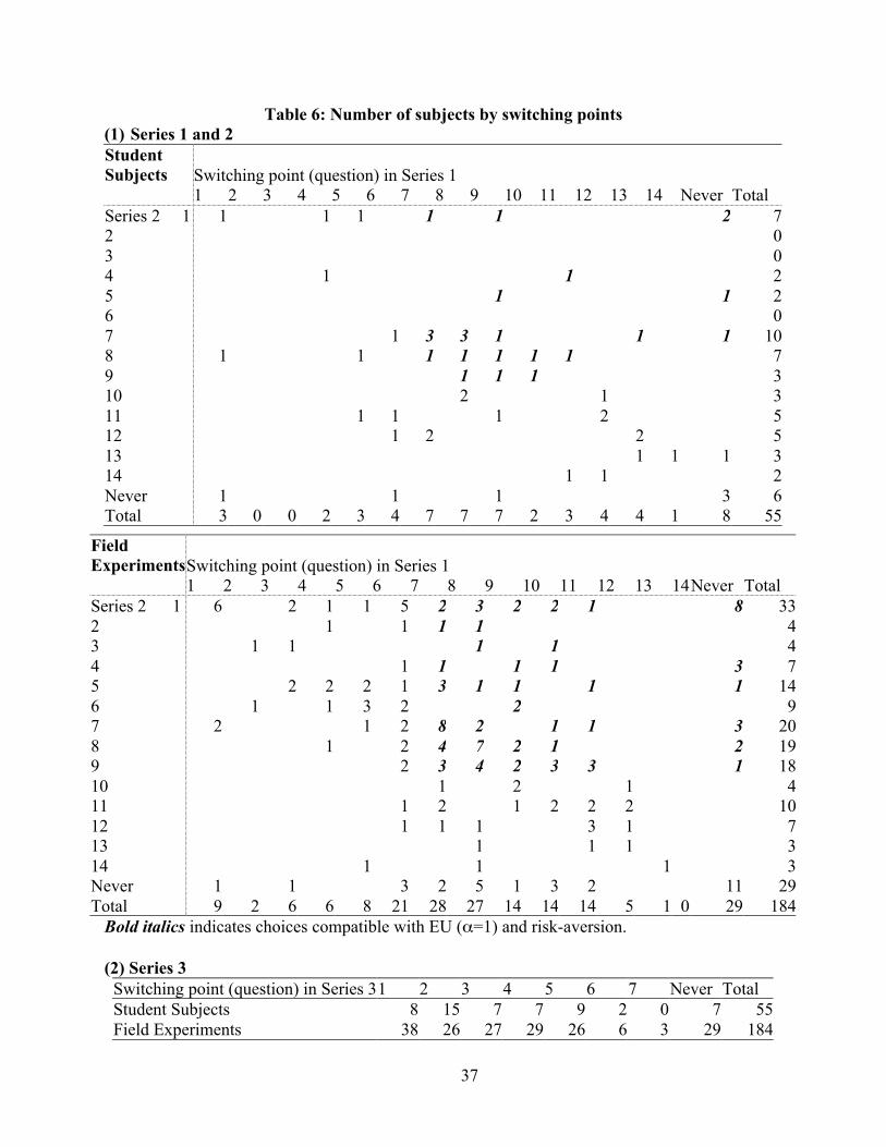
37

Table 6: Number of subjects by switching points(1) Series 1 and 2StudentSubjects Switching point (question) in Series 1

1 2 3 4 5 6 7 8 9 10 11 12 13 14 Never TotalSeries 2 1 1 1 1 1 1 2 72 03 04 1 1 25 1 1 26 07 1 3 3 1 1 1 108 1 1 1 1 1 1 1 79 1 1 1 310 2 1 311 1 1 1 2 512 1 2 2 513 1 1 1 314 1 1 2Never 1 1 1 3 6Total 3 0 0 2 3 4 7 7 7 2 3 4 4 1 8 55

FieldExperimentsSwitching point (question) in Series 1

1 2 3 4 5 6 7 8 9 10 11 12 13 14Never TotalSeries 2 1 6 2 1 1 5 2 3 2 2 1 8 332 1 1 1 1 43 1 1 1 1 44 1 1 1 1 3 75 2 2 2 1 3 1 1 1 1 146 1 1 3 2 2 97 2 1 2 8 2 1 1 3 208 1 2 4 7 2 1 2 199 2 3 4 2 3 3 1 1810 1 2 1 411 1 2 1 2 2 2 1012 1 1 1 3 1 713 1 1 1 314 1 1 1 3Never 1 1 3 2 5 1 3 2 11 29Total 9 2 6 6 8 21 28 27 14 14 14 5 1 0 29 184

Bold italics indicates choices compatible with EU (α=1) and risk-aversion.

(2) Series 3Switching point (question) in Series 31 2 3 4 5 6 7 Never TotalStudent Subjects 8 15 7 7 9 2 0 7 55Field Experiments 38 26 27 29 26 6 3 29 184

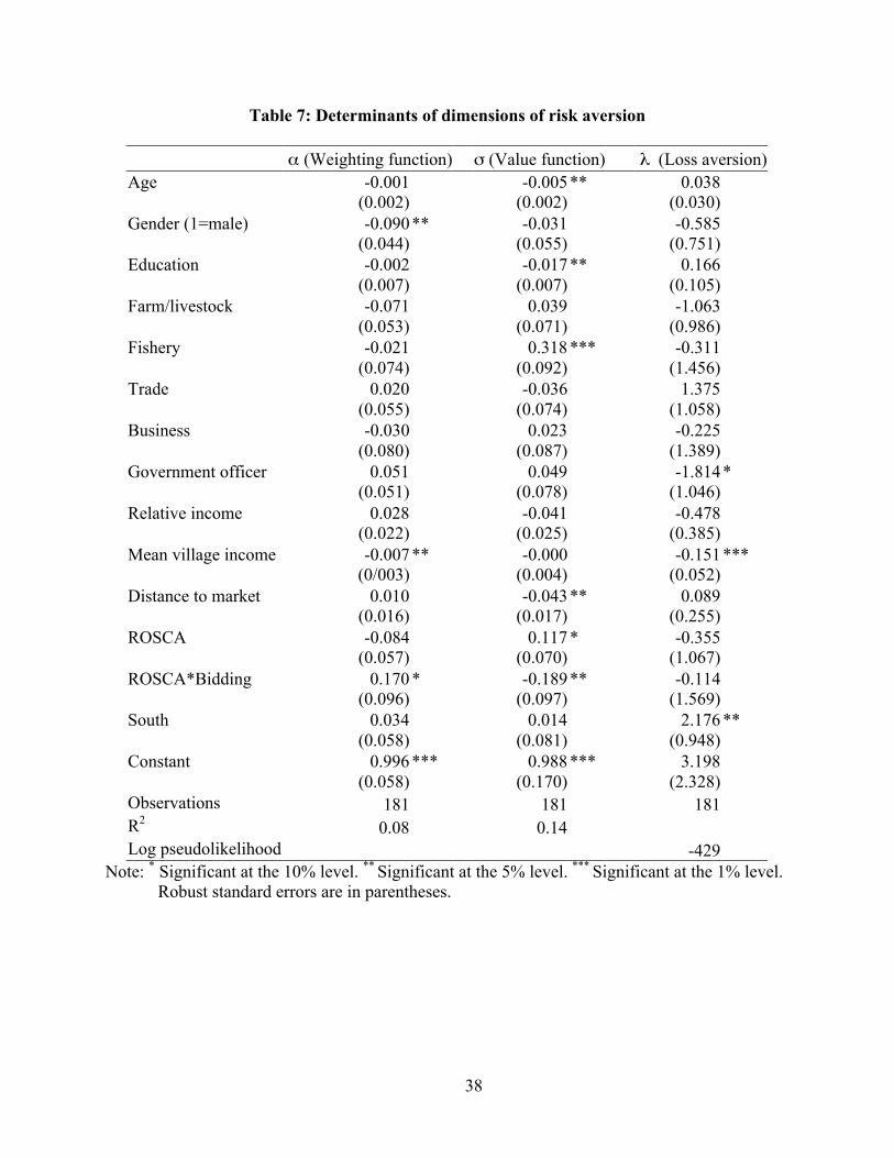
38

Table 7: Determinants of dimensions of risk aversion

α (Weighting function) σ (Value function) λ (Loss aversion)Age -0.001

(0.002)-0.005

(0.002)** 0.038

(0.030)Gender (1=male) -0.090

(0.044)** -0.031

(0.055)-0.585

(0.751)Education -0.002

(0.007)-0.017

(0.007)** 0.166

(0.105)Farm/livestock -0.071

(0.053)0.039

(0.071)-1.063

(0.986)Fishery -0.021

(0.074)0.318

(0.092)*** -0.311

(1.456)Trade 0.020

(0.055)-0.036

(0.074)1.375

(1.058)Business -0.030

(0.080)0.023

(0.087)-0.225

(1.389)Government officer 0.051

(0.051)0.049

(0.078)-1.814

(1.046)*

Relative income 0.028(0.022)

-0.041(0.025)

-0.478(0.385)

Mean village income -0.007(0/003)

** -0.000(0.004)

-0.151(0.052)

***

Distance to market 0.010(0.016)

-0.043(0.017)

** 0.089(0.255)

ROSCA -0.084(0.057)

0.117(0.070)

* -0.355(1.067)

ROSCA*Bidding 0.170(0.096)

* -0.189(0.097)

** -0.114(1.569)

South 0.034(0.058)

0.014(0.081)

2.176(0.948)

**

Constant 0.996(0.058)

*** 0.988(0.170)

*** 3.198(2.328)

Observations 181 181 181R2 0.08 0.14Log pseudolikelihood -429

Note: * Significant at the 10% level. ** Significant at the 5% level. *** Significant at the 1% level.Robust standard errors are in parentheses.

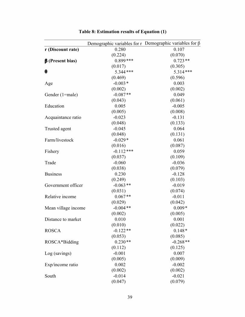
39

Table 8: Estimation results of Equation (1)

Demographic variables for r Demographic variables for βr (Discount rate) 0.280

(0.224)0.107

(0.070)β (Present bias) 0.899

(0.017)*** 0.723

(0.305)**

θ 5.344(0.469)

*** 5.314(0.596)

***

Age -0.003(0.002)

* 0.003(0.002)

Gender (1=male) -0.087(0.043)

** 0.049(0.061)

Education 0.005(0.005)

-0.005(0.008)

Acquaintance ratio -0.023(0.048)

-0.131(0.133)

Trusted agent -0.045(0.048)

0.064(0.131)

Farm/livestock -0.029(0.016)

* 0.061(0.087)

Fishery -0.112(0.037)

*** 0.059(0.109)

Trade -0.060(0.038)

-0.036(0.079)

Business 0.230(0.249)

-0.128(0.103)

Government officer -0.063(0.031)

** -0.019(0.074)

Relative income 0.067(0.029)

** -0.011(0.042)

Mean village income -0.004(0.002)

** 0.009(0.005)

*

Distance to market 0.010(0.010)

0.001(0.022)

ROSCA -0.122(0.053)

** 0.148(0.085)

*

ROSCA*Bidding 0.230(0.112)

** -0.268(0.125)

**

Log (savings) -0.001(0.005)

0.007(0.009)

Exp/income ratio 0.002(0.002)

-0.002(0.002)

South -0.014(0.047)

-0.021(0.079)

40

Observations 2355 2355R2 0.79 0.78

Note: * Significant at the 10% level. ** Significant at the 5% level. *** Significant at the 1% level.We conducted robust regressions, and adjusted standard errors for correlations withinindividuals. 312 data points with inconsistent answers are excluded from the estimations.Robust standard errors are in parentheses.

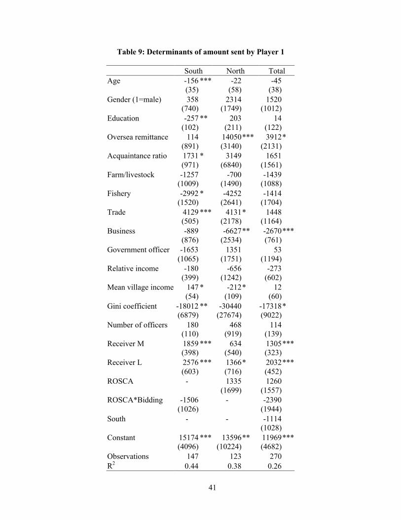
41

Table 9: Determinants of amount sent by Player 1

South North TotalAge -156

(35)*** -22

(58)-45

(38)Gender (1=male) 358

(740)2314

(1749)1520

(1012)Education -257

(102)** 203

(211)14

(122)Oversea remittance 114

(891)14050(3140)

*** 3912(2131)

*

Acquaintance ratio 1731(971)

* 3149(6840)

1651(1561)

Farm/livestock -1257(1009)

-700(1490)

-1439(1088)

Fishery -2992(1520)

* -4252(2641)

-1414(1704)

Trade 4129(505)

*** 4131(2178)

* 1448(1164)

Business -889(876)

-6627(2534)

** -2670(761)

***

Government officer -1653(1065)

1351(1751)

53(1194)

Relative income -180(399)

-656(1242)

-273(602)

Mean village income 147(54)

* -212(109)

* 12(60)

Gini coefficient -18012(6879)

** -30440(27674)

-17318(9022)

*

Number of officers 180(110)

468(919)

114(139)

Receiver M 1859(398)

*** 634(540)

1305(323)

***

Receiver L 2576(603)

*** 1366(716)

* 2032(452)

***

ROSCA - 1335(1699)

1260(1557)

ROSCA*Bidding -1506(1026)

- -2390(1944)

South - - -1114(1028)

Constant 15174(4096)

*** 13596(10224)

** 11969(4682)

***

Observations 147 123 270R2 0.44 0.38 0.26

42

Note: * Significant at the 10% level. ** Significant at the 5% level. *** Significant at the 1% level.We conducted robust regressions, and adjusted standard errors for correlations withinindividuals. Robust standard errors are in parentheses.

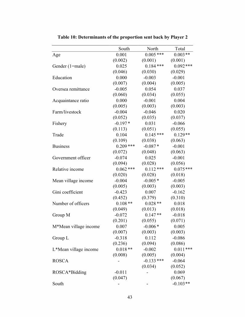
43

Table 10: Determinants of the proportion sent back by Player 2

South North TotalAge 0.001

(0.002)0.005

(0.001)*** 0.003

(0.001)**

Gender (1=male) 0.025(0.046)

0.184(0.030)

*** 0.092(0.029)

***

Education 0.000(0.007)

-0.003(0.004)

-0.001(0.005)

Oversea remittance -0.005(0.060)

0.054(0.034)

0.037(0.055)

Acquaintance ratio 0.000(0.005)

-0.001(0.003)

0.004(0.003)

Farm/livestock -0.004(0.052)

-0.046(0.035)

0.020(0.037)

Fishery -0.197(0.113)

* 0.031(0.051)

-0.066(0.055)

Trade 0.104(0.109)

0.145(0.038)

*** 0.129(0.063)

**

Business 0.209(0.072)

*** -0.087(0.048)

* -0.001(0.063)

Government officer -0.074(0.094)

0.025(0.028)

-0.001(0.056)

Relative income 0.062(0.020)

*** 0.112(0.028)

*** 0.075(0.018)

***

Mean village income -0.004(0.005)

-0.005(0.003)

* -0.005(0.003)

Gini coefficient -0.423(0.452)

0.007(0.379)

-0.162(0.310)

Number of officers 0.108(0.049)

** 0.028(0.013)

** 0.018(0.018)

Group M -0.072(0.201)

0.147(0.055)

** -0.018(0.071)

M*Mean village income 0.007(0.007)

-0.006(0.003)

* 0.005(0.003)

Group L -0.318(0.236)

0.112(0.094)

-0.086(0.086)

L*Mean village income 0.018(0.008)

** -0.002(0.005)

0.011(0.004)

***

ROSCA - -0.133(0.034)

*** -0.064(0.052)

ROSCA*Bidding -0.011(0.047)

- 0.069(0.067)

South - - -0.103**

44

(0.047)Constant 0.123

(0.354)0.007

(0.177)0.141

(0.181)Observations 490 420 910R2 0.22 0.51 0.27

Note: * Significant at the 10% level. ** Significant at the 5% level. *** Significant at the 1% level.We conducted robust regressions, and adjusted standard errors for correlations withinindividuals. Robust standard errors are in parentheses.

45

Table 11: Correlation between risk, time discounting and trust

σ λMeandiscountfactor

Mean amountsent(Player 1)

Mean return rate(Player 2)

α 0.19** 0.03 -0.09 -0.26** -0.06σ -0.13* -0.05 -0.15 -0.00λ -0.05 -0.11 -0.11Mean discountfactor -0.02 -0.02

Note: * Significant at the 10% level. ** Significant at the 5% level.

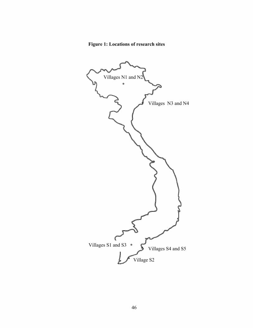
46

Figure 1: Locations of research sites

Villages N1 and N2*

Villages N3 and N4*

Villages S4 and S5*Villages S1 and S3 *

Village S2*

47

Figure 2: Cumulative distribution of amount sent by Player 1 (by group of receiver).Players in South send less (lower medians) and send more to group L than to groups M andH, compared to players in North.

South North

0

0.2

0.4

0.6

0.8

1

0 2 4 6 8 10 12 14 16 18 20Amount sent (1000 dong)

Receiver: Group H Receiver: Group MReceiver: Group L p=.5

0.00

0.20

0.40

0.60

0.80

1.00

0 2 4 6 8 10 12 14 16 18 20Amount sent (1000 dong)

Receiver: Group H Receiver: Group MReceiver: Group L p=.5

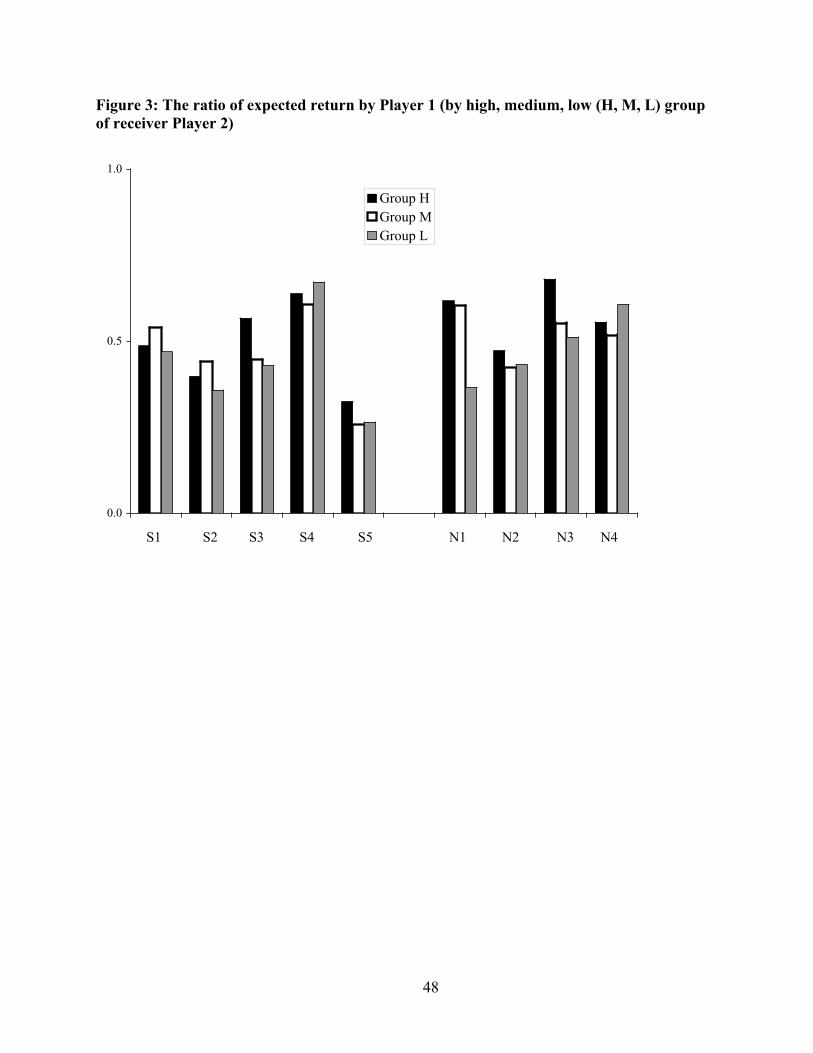
48

Figure 3: The ratio of expected return by Player 1 (by high, medium, low (H, M, L) groupof receiver Player 2)

0.0

0.5

1.0

Group HGroup MGroup L

S1 S2 S3 S4 S5 N1 N2 N3 N4

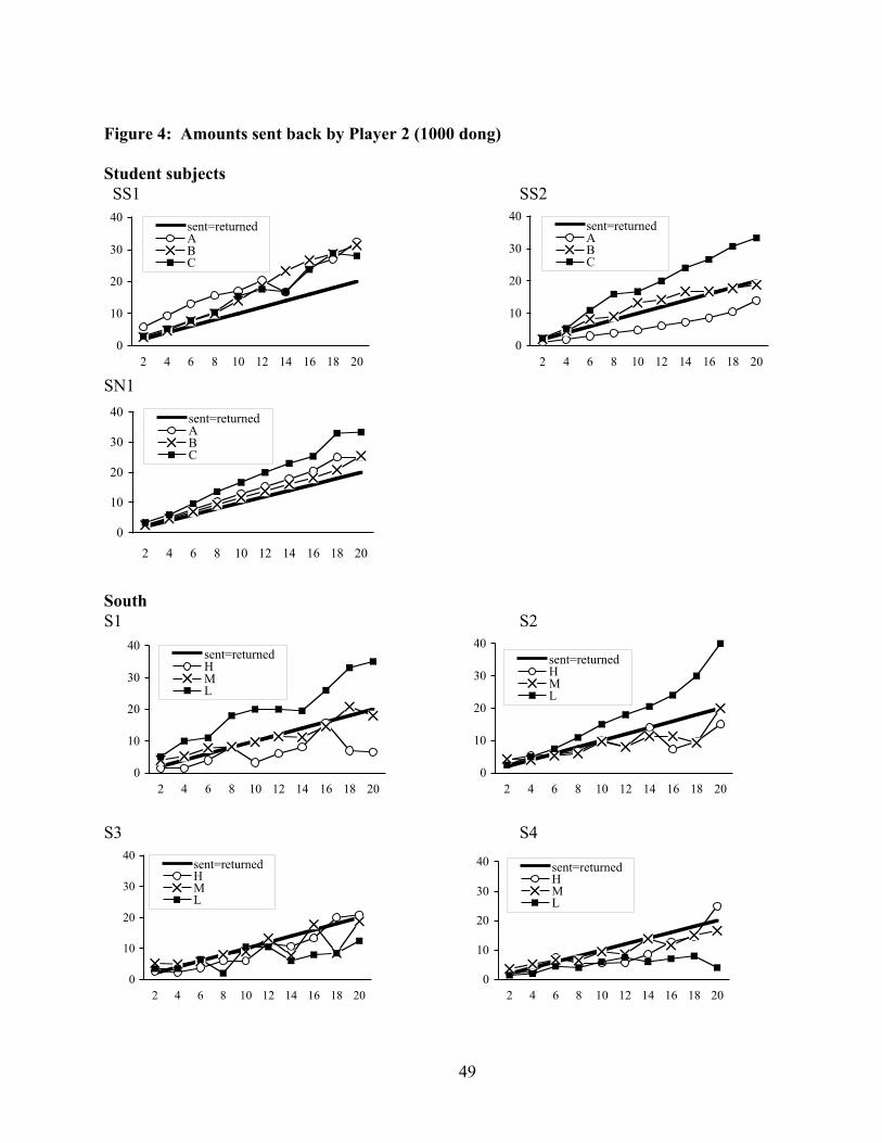
49

Figure 4: Amounts sent back by Player 2 (1000 dong)

Student subjects SS1 SS2

0

10

20

30

40

2 4 6 8 10 12 14 16 18 20

sent=returnedABC

0

10

20

30

40

2 4 6 8 10 12 14 16 18 20

sent=returnedABC

SN1

0

10

20

30

40

2 4 6 8 10 12 14 16 18 20

sent=returnedABC

SouthS1 S2

0

10

20

30

40

2 4 6 8 10 12 14 16 18 20

sent=returnedHML

0

10

20

30

40

2 4 6 8 10 12 14 16 18 20

sent=returnedHML

S3 S4

0

10

20

30

40

2 4 6 8 10 12 14 16 18 20

sent=returnedHML

0

10

20

30

40

2 4 6 8 10 12 14 16 18 20

sent=returnedHML

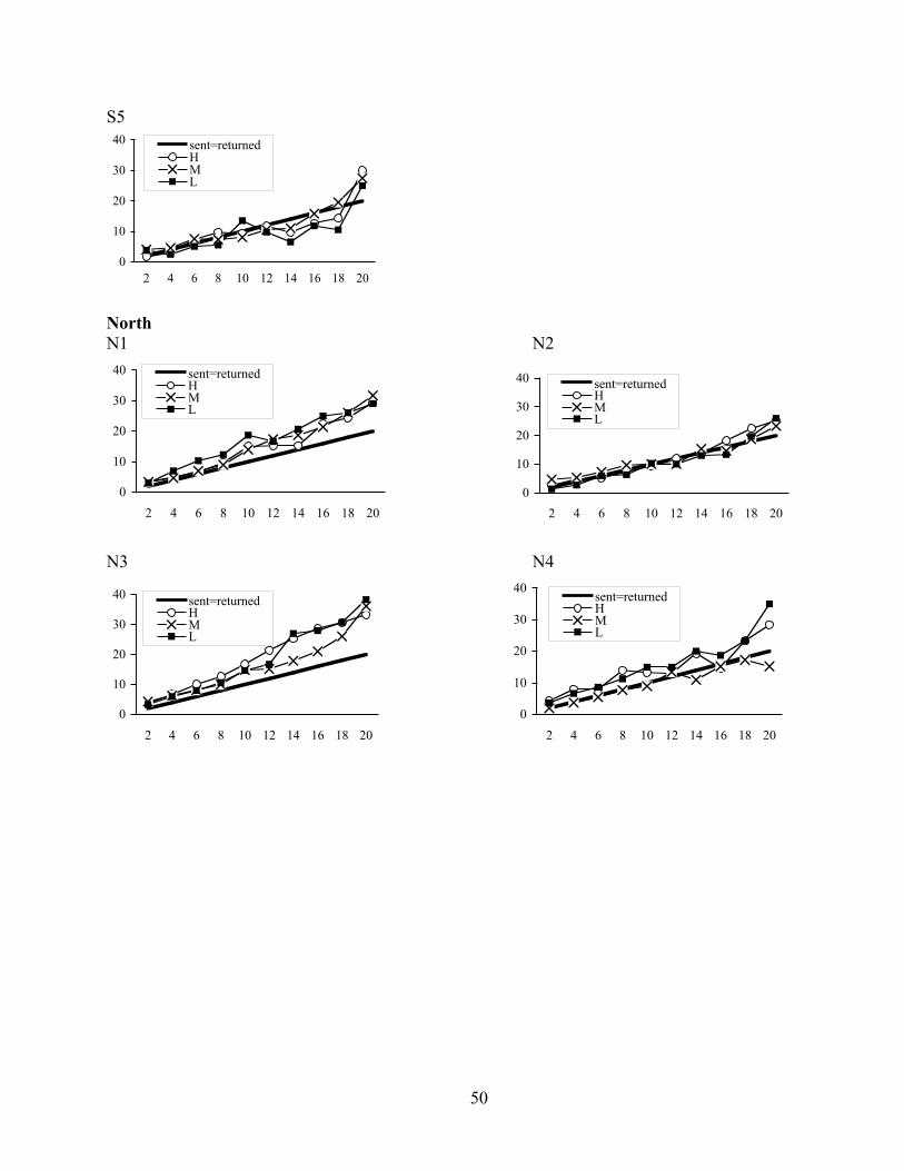
50

S5

0

10

20

30

40

2 4 6 8 10 12 14 16 18 20

sent=returnedHML

NorthN1 N2

0

10

20

30

40

2 4 6 8 10 12 14 16 18 20

sent=returnedHML

0

10

20

30

40

2 4 6 8 10 12 14 16 18 20

sent=returnedHML

N3 N4

0

10

20

30

40

2 4 6 8 10 12 14 16 18 20

sent=returnedHML

0

10

20

30

40

2 4 6 8 10 12 14 16 18 20

sent=returnedHML