Experimental and numerical investigations of a...

Linköping Studies in Science and Technology Dissertation No. 1606

Experimental and numerical investigations of a ventilation strategy – impinging jet ventilation for an

office environment

Huijuan Chen

Division of Energy Systems Department of Management and Engineering

Linköping University SE-581 83 Linköping, Sweden

2014

II

Copyright © Huijuan Chen 2014, unless otherwise noted. ISBN: 978-91-7519-299-4 ISSN: 0345-7524 Printed in Sweden by LiU-Tryck, Linköping 2014.

III

ABSTRACT

A well-functioning, energy-efficient ventilation system is of vital importance to offices, not only to provide the kind of comfortable, healthy indoor environment necessary for the well-being and productive work performance of occupants, but also to reduce energy use in buildings and the associated impact of CO2 emissions on the environment. To achieve these goals impinging jet ventilation has been developed as an innovative ventilation concept. In an impinging jet ventilation system, a high momentum of air jet is discharged downwards, strikes the floor and spreads over it, thus distributing the fresh air along the floor in the form of a very thin shear layer. This system retains advantages of mixing and stratification from conventional air distribution methods, while capable of overcoming their shortcomings. The aim of this thesis is to reach a thorough understanding of impinging jet ventilation for providing a good thermal environment for an office, by using Computational Fluid Dynamics (CFD) supported by detailed measurements. The full-field measurements were carried out in two test rooms located in a large enclosure giving relatively stable climate conditions. This study has been divided into three parts where the first focuses on validation of numerical investigations against measurements, the second addresses impacts of a number of design parameters on the impinging jet flow field and thermal comfort level, and the third compares ventilation performance of the impinging jet supply device with other air supply devices intended for mixing, wall confluent jets and displacement ventilation, under specific room conditions. In the first part, velocity and temperature distributions of the impinging jet flow field predicted by different turbulence models are compared with detailed measurements. Results from the non-isothermal validation studies show that the accuracy of the simulation results is to a great extent dependent on the complexity of the turbulence models, due to complicated flow phenomena related to jet impingement, such as

recirculation, curvature and instability. The fv 2 turbulence model shows the best

performance with measurements, which is slightly better than the SST k-ω model but much better than the RNG k-ε model. The difference is assumed to be essentially related to the magnitude of turbulent kinetic energy predicted in the vicinity of the stagnation region. Results from the isothermal study show that both the SST k-ω and RNG k-ε models predict similar wall jet behaviours of the impinging jet flow.

IV

In the second part, three sets of parametric studies were carried out by using validated CFD models. The first parametric study shows that the geometry of the air supply system has the most significant impact on the flow field. The rectangular air supply device, especially the one with larger aspect ratio, provides a longer penetration distance to the room, which is suitable for industrial ventilation. The second study reveals that the interaction effect of cooling ceiling, heat sources and impinging jet ventilation results in complex flow phenomena but with a notable feature of air circulation, which consequently decreases thermal stratification in the room and increases draught discomfort at the foot level. The third study demonstrates the advantage of using response surface methodology to study simultaneous effects on changes in four parameters, i.e. shape of air supply device, jet discharge height, supply airflow rate and supply air temperature. Analysis of the flow field reveals that at a low discharge height, the shape of air supply device has a major impact on the flow pattern in the vicinity of the supply device. Correlations between the studied parameters and local thermal discomfort indices were derived. Supply airflow rates and temperatures are shown to be the most important parameter for draught and stratification discomfort, respectively. In the third part, the impinging jet supply device was shown to provide a better overall performance than other air supply devices used for mixing, wall confluent jets and displacement ventilation, with respect to thermal comfort, heat removal effectiveness, air exchange efficiency and energy-saving potential related to fan power.

V

SAMMANFATTNING

Ett väl fungerande, energieffektivt ventilationssystem är av avgörande betydelse för ett kontor. Inte bara för att det behövs en komfortabel och hälsosam inomhusmiljö för de människors välbefinnande och produktivitet, utan även för att minska energianvändningen i byggnaden och för att reducera CO2 utsläppen med dess påverkan på klimatet. För att uppnå dessa mål har impinging jet ventilation utvecklats som ett nytt innovativt ventilationskoncept. Det nya systemet bygger på att en friströmmande luftstråle tillförs längs en vägg vinkelrätt mot golvet. Efter nerslaget mot golvet sprids den friska luften längs golvet i form av ett mycket tunt skikt. Detta system bibehåller fördelarna med traditionella ventilationsmetoder, men har dessutom en potential att ytterligare förbättra inomhusklimatet och använda mindre energi. Syftet med denna studie är att ge en grundlig förståelse av hur impinging jet ventilation kan skapa god termisk komfort i kontorslokaler genom Computational Fluid Dynamics (CFD)-simulering med stöd av detaljerade mätningar. Dessa mätningar genomfördes i två olika testrum i en kontrollerad laboratoriemiljö. Denna studie består av tre delar där den första delen fokuserar på validering av numeriska beräkningar mot mätningar, den andra delen tar upp effekterna av ett antal parametrar på flödesfält och termisk komfort, och den tredje jämför prestanda för detta system med prestanda för andra ventilationssystem. I den första delen valideras olika turbulensmodeller mot detaljerade mätningar för hastighet och temperatur. Resultaten från den icke-isotermiska studien visar att turbulensmodeller är av central betydelse för noggrannheten i simuleringsresultaten, beroende på komplicerade strömningsmekanismer kopplade till impingementeffekten.

Bäst överensstämmelse med mätningar visar fv 2 modellen, klart bättre än SST k-ω

och mycket bättre än RNG k-ε. Resultaten från det isotermiska fallet visar att SST k-ω och RNG k-ε modellerna har liknande prestanda. I den andra delen genomfördes en parametersstudie med hjälp av de validerade modellerna. Den första parametriska studien visar att lufttilldonets utformning har störst inverkan på strömningsfältet. Den andra studien visar att interaktionseffekten av kyltak, värmekällor och impinging jet ventilation ger komplexa strömningsfenomen som kraftigt påverkar luftcirkulationen och ger golvdrag, vilket minskar den termiska komforten. Den tredje studien visar fördelarna med att använda Response Surface Methodology för att studera samtidiga effekter av förändringar i fyra parametrar:

VI

tilluftdonet, donhöjden, tilluftsflödet och tilluftstemperaturen. Korrelationen mellan de studerade parametrarna och ett antal inomhusklimatindex härleddes. I den tredje delen jämfördes ventilationsprestanda för impinging jet ventilation med andra vanligt förekommande system under specifika rumsförhållanden. Impinging jet ventilation visade bättre prestanda än andra system avseende termisk komfort, borttagning av interna och externa värmelaster, luftutbyteseffektivitet och möjligheter att spara energi i samband med fläkteffekten.

VII

ACKNOWLEDGEMENTS

I would like to thank my supervisor, Professor Bahram Moshfegh, for introducing me to the world of scientific research and for his valuable guidance, encouragement and support during the development of this work. I would also like to thank my assistant supervisor, Dr. Mathias Cehlin, for his support, kindness, insight and suggestions on this thesis. I will forever be thankful to them for helping me develop on both an academic and a personal level during these years. I would also wish to thank Professor Hazim Awbi, at Reading University, U.K. for the discussions on my research and valuable comments on drafts of the thesis. I am also grateful to the financial support from Formas (contract number 242-2008-835), KK Foundation (contract number 2007/0289), System Air AB, Kraft and Kultur AB, University of Gävle (Gävle, Sweden), and Linköping University (Linköping, Sweden). I would like to express my sincere gratitude to Tech. lic. Hans Lundström, who has been directly involved in laboratory work of this thesis. I thank him for technical help, much valuable advice, insightful discussions, and great effort on repairing hot-wire sensors. Special thanks also go to Dr. Claes Blomqvist for valuable suggestions on velocity measurements, as well as to Mr. Ragnvald Pelttari and Mr. Richard Larsson for their careful set-ups of the test room. Appreciations also go to Associate Professor Patrik Rohdin, at Linköping University, for help on thermal comfort calculation, Ms. Elisabeth Larsson and Ms. Lena Sjöholm for all administrative help, and PhD student Linn Liu for help and friendship. I also want to thank all my colleagues at the Department of Building, Energy and Environmental Engineering in Gävle. Without you my time as a PhD student would have been less productive and joyful. I especially want to thank Tech. lic. Ulf Larsson, Dr. Håkan Attius, Associate Professor Karimipanah Taghi, Dr. Nawzad Mardan, and PhD student Gottfried Weinberger for the inspiring talk, continued encouragement and support. Special thanks also go to Mr. Staffan Nygren, Ms. Eva Wännström and Ms. Malin Ekeberg for always being so kind and helpful. Finally, I would like to thank my parents, for their constant and unconditional love, support and motivation. I also want to thank my friends, for joyful moments and moral support during these years.

IX

LIST OF APPENDED PAPERS

The doctoral thesis is based on the following papers which are listed in accordance with the research process. Paper I Chen, H. J., Moshfegh, B., & Cehlin, M. (2012). Numerical investigation

of the flow behaviour of an isothermal impinging jet in a room. Building and Environment, 49, 154-166.

Paper II Chen, H. J., & Moshfegh, B. (2011). Comparing k-ε models on predictions

of an impinging jet for ventilation of an office room. Proceedings of the 12th International Conference on Air Distributions in Rooms, Trondheim, Norway.

Paper III Chen, H. J., Moshfegh, B., & Cehlin, M. (2013). Investigation on the flow

and thermal behaviour of impinging jet ventilation systems in an office with different heat loads. Building and Environment, 59, 127-144.

Paper IV Chen, H. J., Moshfegh, B., & Cehlin, M. (2013). Computational

investigation on the factors influencing thermal comfort for impinging jet ventilation. Building and Environment, 66, 29-41.

Paper V Chen, H. J., Janbakhsh, S., Larsson, U, & Moshfegh, B. Comparisons of

ventilation performances of different air supply devices in an office environment. Submitted for journal publication.

XI

NOMENCLATURE

AR Aspect ratio, (-) Co Number of centre points, (-) C1, C2, C1ε, C2ε, C3ε, C1k, C2k, CL, Ct , Cμ, Ck,1, Ck,2

Cω,1, Cω,2, Coefficients in turbulence models, (-) cp Specific heat at constant pressure, (J/kg·°C)

dh Hydraulic diameter, (m) F1 Blending function, (-) f Elliptic relaxation factor, (-) fcl Clothing surface area factor, (-) Gk Production of turbulent energy, (W/m3) g Gravity, (m/s2) H Jet discharge height, (m) hc Convective heat transfer coefficient, (W/m2·°C)

Icl Clothing insulation, (m2·°C/W) k Thermal conductivity, (W/m·°C)

Turbulent kinetic energy, (m2/s2) and Number of factors, (-) l Length scale, (m) M Metabolism, (W/m2) N Total number of runs, (-) n Local coordinate normal to the wall, (-) P Pressure, (Pa) pa Water vapour partial pressure, (Pa) Pr = ν/α Prandtl number, (-) Q Supply airflow rate, (m3/s) Re Reynolds number, (-) Sij Rate-of-strain tensor, (1/s) T Turbulent time scale, (s) Ts Supply air temperature, (°C)

Tu Turbulence intensity, (-) ta Air temperature, (°C) tcl Clothing surface temperature, (°C)

rt Mean radiant temperature, (°C) U Mean velocity, (m/s) Ui = (U, V, W) Mean velocity component, (m/s) u Velocity, (m/s) ui = (u, v, w) Instantaneous velocity component, (m/s)

XII

uτ Viscous velocity, (m/s) u´ Fluctuating velocity, (m/s)

iu = (u´, v´, w´) Fluctuating velocity component, (m/s)

var Relative air velocity, (m/s) 2v Wall normal Reynolds stress component, (m2/s2)

W External work, (W/m2) Xi Coded variable, (-) xi Independent variable, (-) xi = (x, y, z) Cartesian coordinate, (m) Y Response variable, (-) y Normal distance to the wall, (m) y+ Dimensionless distance from the wall, (-) Greek symbols α Thermal diffusivity, (m2/s) and Relaxation factor, (-) β Volumetric thermal expansion coefficient, (1/K) βi Regression coefficients for the linear terms, (-) βii Regression coefficients for the quadratic terms, (-) βij Regression coefficients for the interaction terms, (-) βo Model intercept coefficient, (-) δij Kronecker delta function, (-) ε Rate of dissipation of turbulent kinetic energy, (m2/s3) and Emissivity, (-) εt Heat removal effectiveness, (-) εa Air exchange efficiency, (-) ϕ General scalar variable, (-) κ Von Karman constant, (-) λε Blending function, (-) μ Dynamic viscosity, (kg/m·s) μt Turbulent viscosity, (kg/m·s) ν Kinematic viscosity, (m/s2) Θ Time averaged temperature, (°C)

θ Instantaneous temperature, (°C)

θ΄ Fluctuating temperature, (C) ρ Density, (kg/m3) ρo Reference density, (kg/m3) σk, σε, σt Turbulent Prandtl number, (-) τw Wall shear stress, (N/m2) ω Turbulence frequency, (1/s)

XIII

TABLE OF CONTENTS

1. INTRODUCTION ...................................................................................................... 1

1.1 Background ............................................................................................................. 1

1.2 Motivation of this study .......................................................................................... 2

1.3 Aim and research process ....................................................................................... 2

1.4 Research methods ................................................................................................... 3

1.5 Limitations .............................................................................................................. 4

1.6 Summary of the appended papers ........................................................................... 4

1.7 Co-author statements .............................................................................................. 7

2. INDOOR ENVIRONMENT AND VENTILATION SYSTEMS ........................... 9

2.1 Thermal comfort ..................................................................................................... 9

2.1.1 Overall thermal comfort ................................................................................... 9

2.1.2 Local thermal discomfort ............................................................................... 11

2.2 Indoor air quality .................................................................................................. 12

2.3 Ventilation effectiveness ....................................................................................... 13

2.4 Air distribution systems ........................................................................................ 14

2.4.1 Impinging jet ventilation ................................................................................ 16

3. LITERATURE REVIEW ........................................................................................ 19

3.1 Impinging jet ......................................................................................................... 19

3.2 Impinging jet ventilation ....................................................................................... 22

4. METHODS ................................................................................................................ 25

4.1 Measuring methods for velocities and temperatures ............................................ 25

4.1.1 Whole-field measuring techniques ................................................................. 26

4.1.2 Point-measuring methods ............................................................................... 27

4.1.2.1 Thermal anemometers ............................................................................. 27

4.2 Experimental set-up .............................................................................................. 29

4.2.1 Experimental set-up for the isothermal case .................................................. 29

4.2.1.1 Airflow rate, velocity and temperature measurements ............................ 30

4.2.2 Experimental set-ups for the non-isothermal case ......................................... 33

4.2.2.1 Airflow, velocity and temperature measurements ................................... 34

4.3 Computational fluid dynamics .............................................................................. 36

4.3.1 Governing equations ...................................................................................... 37

4.3.2 Turbulence ...................................................................................................... 38

4.3.2.1 Time-averaged transport equations ......................................................... 38

XIV

4.3.3 Computational approaches ............................................................................. 39

4.3.3.1 RANS modelling ..................................................................................... 40

4.3.3.2 Boundary conditions ................................................................................ 46

4.3.3.3 Near-wall treatments ............................................................................... 47

4.3.3.4 Mesh strategies ........................................................................................ 50

4.3.3.5 Numerical aspects .................................................................................... 51

4.4 Statistical approximation approach ....................................................................... 53

4.4.1 Response surface methodology ...................................................................... 54

4.4.1.1 Determination of independent variables and their levels ........................ 55

4.4.1.2 Experimental design ................................................................................ 55

4.4.1.3 Establishment of the response surface model and verification ................ 57

4.4.1.4 Graphical presentation of the response surface model and optimization 58

5. RESULTS AND DISCUSSION ............................................................................... 59

5.1 CFD validation results .......................................................................................... 59

5.1.1 Isothermal case ............................................................................................... 59

5.1.2 Non-isothermal case ....................................................................................... 61

5.2 Parametric studies ................................................................................................. 63

5.2.1 Parametric study (one-factor-at-a-time): part one .......................................... 63

5.2.2 Parametric study (one-factor-at-a-time): part two .......................................... 64

5.2.3 Parametric study (based on response surface methodology): part three ........ 67

5.3 Ventilation performance comparison .................................................................... 69

6. CONCLUSIONS ....................................................................................................... 73

6.1 Validation study .................................................................................................... 73

6.2 Parametric study ................................................................................................... 74

6.3 Ventilation performance comparison study .......................................................... 74

7. FUTURE WORK ...................................................................................................... 77

REFERENCES ............................................................................................................. 79

1

1. INTRODUCTION

1.1 Background

Indoor environmental conditions are important to the health, comfort and productivity of occupants. Accumulating evidence has shown that poor climate quality is related to increased sick building syndrome (SBS) symptoms and decreased work performance (Seppanen and Fisk, 2006). Recent studies by Lan et al. (2011) and Tsai et al. (2012) reported that thermal discomfort and high indoor carbon dioxide concentrations increase SBS symptoms for office workers. Ventilation systems are therefore widely used to provide a good indoor environment with respect to thermal comfort and indoor air quality. By delivering a sufficient amount of outdoor cool fresh air into the room, excess heat and internally generated contaminant concentration levels can be removed and reduced. Natural ventilation appeared as an attractive strategy used in the past to provide an acceptable microclimate in the space being ventilated (Busch, 1992), but it is limited to range of climates, microclimates, building types, etc. (Allocca et al., 2003). To enhance control of indoor climate, mechanical ventilation is desirable, which can be used for different types of buildings and offers more possibilities to regulate room air temperature, humidity, air speed and contaminants. A properly designed ventilation system could contribute to the promotion of occupants’ performance and the reduction of airborne infectious diseases (Seppänen, 2008).

As a result of energy-saving measures stimulated by the energy crisis in the early 1970s, there was a trend to construct better insulated, more airtight buildings. One of the consequences was that the air supplied to the space for maintaining a comfortable temperature is reduced. However, such a reduction of ventilation rate could aggravate the deterioration of the indoor air quality, particularly nowadays with large amounts of synthetic materials and chemical products being used indoors. In addition, inadequate ventilation rates sometimes generate poor distribution of indoor air flow, temperature and contaminant concentration in the occupied zone, which might consequently cause problems for the indoor environment (Chen and Glicksman, 2003). Moreover, in a modern society, people spend most of their time indoors where they perform the major activities of working and living. Combined this leads to an increasing dependency for the desired indoor environment of buildings on ventilation and air-conditioning systems. In today’s office environment, computers and other heat-generating devices are widely used, and these internal heat gains together with intense solar conditions can result in a high heat load in enclosures. This poses challenges for office ventilation.

2

Meanwhile, ventilation systems account for a large part of the total energy usage in the residential and service sector in Sweden (SEA, 2012). Sweden has set up national goals related to the European Union’s climate and energy goals, and energy use in the building sector must be reduced by 20% by 2020 and 50% in residential and commercial buildings by 2050 compared to 1995 (SEA, 2012). Decreasing energy use in the building sector is a key factor to manage the national goals for reduction of CO2 emissions. Therefore effective ventilation systems have to be used not only to provide a healthy indoor climate but also to contribute to reduction in energy usage. At present, conventional mixing and displacement ventilation are still most widely used, though they have some disadvantages and limitations. To overcome the drawbacks of these systems while retaining the strengths they provide, impinging jet ventilation (IJV) was proposed by Karimipanah and Awbi (2002) to be used for space ventilation, cooling and heating. This system combines positive aspects of mixing and displacement ventilation and therefore has a promising application.

1.2 Motivation of this study

As addressed in section 1.1, ventilation systems play an important role in thermal comfort, indoor air quality and energy usage. It is of great importance to develop innovative air distribution systems such as IJV, which have great potential to provide an acceptable indoor environment while using energy efficiently.

1.3 Aim and research process

The aim of this thesis is to reach a thorough understanding of implementation of the impinging jet (IJ) principle to space ventilation for providing a good office environment, by using computational fluid dynamics (CFD) simulations supported by measurements. To be more specific, this study aims to investigate the flow field and thermal behaviour of IJV as well as the system performance regarding thermal comfort and ventilation effectiveness in an office environment. The research process consists of three parts as shown below: – Validation studies – Parametric studies

Strategy 1: only considering effects caused by one parameter at a time, known as one-variable-at-a-time strategy.

3

Strategy 2: considering simultaneous effect of changes in two or more parameters on results.

– Ventilation performance comparisons In the first part (Paper I, II and III), numerical models are validated against detailed measurements with almost identical set-up. Velocity and temperature distributions predicted by CFD are compared with measured values at various locations in the room. Effects of turbulence modelling and grid density on the prediction accuracy are examined. One outcome of the validation study is to obtain a reliable turbulence model for parametric studies. Flow characteristics of IJ are also discussed. In the second part, influences of the parameters with respect to the configuration of IJ device, air supply conditions and room design parameters (e.g. room heat sources and cooling ceiling) on flow and temperature fields and thermal comfort are investigated, based on a validated CFD program. Two strategies are used in the parametric studies: the first is based on one-factor-at-a-time (Paper I and III) while the second (Paper IV) considers simultaneous effects of changes in two or more parameters on the results with the use of a statistical technique called Response Surface Methodology. In the third part (Paper V), performance of the impinging jet supply device is compared with other air supply devices intended for mixing, wall confluents jets and displacement ventilation by performing CFD simulations. Results are focused on thermal comfort, heat removal effectiveness, air exchange efficiency and energy-saving potential.

1.4 Research methods

Two main methods are used to carry out this research, measurements and CFD simulations. The main focus is on CFD simulations; measurements are used to provide boundary conditions and validate different CFD models. Based on the validated models, an extensive parametric study is performed to investigate influences of a number of parameters on the flow field, thermal behaviour and related thermal comfort level of IJV in an office environment, with an ultimate goal of maximizing the system performance. The response surface methodology is also used to provide a systemic and efficient strategy for parametric studies.

4

1.5 Limitations

The investigation of IJV in this study is limited to office environment with a focus on velocity and temperature fields as well as thermal comfort. The measurements intended for the validation of the CFD method are limited to hot-wire and hot-sphere anemometers, which consists of high uncertainties when measuring flows with high turbulence or low velocities. The CFD study is limited to steady-state and eddy-viscosity turbulence models, due to affordable computational sources, reasonable accuracy and complex geometries of the studied cases. Ventilation efficiency of IJV is assessed with regards to heat removal effectiveness, and air exchange efficiency based on mean age of air calculated by CFD.

1.6 Summary of the appended papers

Paper I Chen, H. J., Moshfegh, B., & Cehlin, M. (2012). Numerical investigation of the flow behaviour of an isothermal impinging jet in a room. Building and Environment, 49, 154-166. This paper presents a numerical study of the characteristics of turbulent impinging jet flow in an empty room by using a CFD program. Influences of different configurations and flow parameters of the newly proposed IJ supply device on the flow field were investigated. The CFD model was validated against detailed hot-wire measurements, and turbulence was modelled by the RNG k-ε and SST k-ω model. Good agreement with measurements was obtained from both turbulence models, and a closer consistency near the impingement zone was observed from the SST k-ω model. Results from case studies based on the SST k-ω model revealed that the flow behaviour is most significantly affected by the geometry of the IJ supply device, while it is affected to some extent by the discharge height in areas close to the air supply device. Paper II Chen, H. J. & Moshfegh, B. (2011). Comparing k-ε models on predictions of an impinging jet for ventilation of an office room. Proceedings of the 12th International Conference on Air Distributions in Rooms, Trondheim, Norway. This paper was presented as a validation study of a CFD program with three versions of k-ε models together with enhanced wall treatments. Experiments were performed in a full-scale test room with dimensions 4.2 × 3.6 × 2.5 m, and furnished like a single-person office equipped with IJV. Detailed velocity and temperature

5

measurements with use of single-sensor hot-wire probe were conducted in regions below the jet exit section and along the floor, lying in the vertical middle plane of the room. Better consistency between predictions and measurements was observed in the free jet region and the wall jet region, and larger deviations were found close to the impingement region due to complex flow features caused by jet impingement. Although the RNG k-ε model shows the least deviation with measurements among the three k-ε models, more complex turbulence models are needed in order to improve prediction accuracies. Paper III Chen, H. J., Moshfegh, B., & Cehlin, M. (2013). Investigation on the flow and thermal behaviour of impinging jet ventilation systems in an office with different heat loads. Building and Environment, 59, 127-144. This paper concerns influences of room design factors on IJV performance by using a CFD program. The main objective of this paper was to explore interaction effects of a cooling ceiling, heat sources and IJV on flow and thermal fields as well as local thermal comfort in an office environment. This study was also a continuation of the validation study from Paper II. In this paper, more complex turbulence models, i.e.

SST k-ω and fv 2 , were employed, and comparisons with measurements were

extended from the jet region to various zones in the room. Results from the validation study showed that velocity and temperature predictions by the RNG k-ε model close to the impingement region were improved by the SST k-ω

model to some extent, while the simulations were greatly improved by the fv 2

model. The fv 2 model gave the best overall agreement with measurements and

therefore was chosen for further studies. Results from case studies indicated that the interaction effect results in a complex flow phenomenon but with a notable feature of air circulation, and the appearance and strength of the air circulation mainly depend on the external heat load on windows and number of occupants. The generated large air circulation consequently alters the temperature field and the local thermal comfort level for IJV. Paper IV Chen, H. J., Moshfegh, B., & Cehlin, M. (2013). Computational investigation on the factors influencing thermal comfort for impinging jet ventilation. Building and Environment, 66, 29-41.

6

This paper demonstrates the benefits of using the response surface methodology coupled with CFD for systematically studying the effects of IJ configuration and air supply parameters on local thermal discomfort. The simultaneous effect of changes in two or more parameters on the result was studied. A total of four parameters were studied, each of which had three levels. The numbers of CFD simulations required for performing such studies were largely reduced with the use of the Box-Behnken design method. The results indicated that at a low discharge height, the shape of air supply device has a major impact on flow patterns close to the supply device, due to the footprint of the impinging jet. This effect consequently affects the draught discomfort in the occupied zone. The response surface methodology analysis highlighted that the supply airflow rate and supply air temperature are the most important parameters influencing the draught discomfort and temperature stratification, respectively. Correlations between the response (i.e. draught and temperature difference) and the parameters studied were also established. Paper V Chen, H. J., Janbakhsh, S., Larsson, U., & Moshfegh, B. Comparisons of ventilation performances of different air supply devices in an office environment. Submitted for journal publication. This paper compared ventilation performance of four air supply devices intended for mixing, wall confluent jets, impinging jet and displacement ventilation in an office environment by performing CFD simulations. Comparisons were made under identical set-up conditions, as well as the same occupied zone temperature of about 24.2 °C achieved by adding different heat loads and using different airflow rates. Results were discussed based on thermal comfort levels, heat removal effectiveness and air exchange efficiency. In addition, energy-saving potential was addressed based on the supply airflow rate and the related fan power required for obtaining a similar occupied zone temperature for each device. Results from the specific case studies showed that the impinging jet supply device could provide an acceptable thermal environment for occupants, as well as showing higher ventilation efficiency than the mixing supply device, in terms of heat removal effectiveness, air exchange efficiency and fan power, as it combined characteristics of both mixing and stratification principles. The displacement supply device presented the highest ventilation efficiency and greatest fan power reduction, but it had difficulties satisfying requirements on local thermal comfort due to large vertical temperature gradients.

7

1.7 Co-author statements

The first, third and fourth papers were written entirely by the author of this thesis, but valuable input and important comments on plans and drafts of these papers were provided by Professor Bahram Moshfegh and Dr. Mathias Cehlin. The second paper was planned, executed and written by the author, but under the supervision of Professor Bahram Moshfegh. The fifth paper was written in collaboration with PhD students Ulf Larsson and Setareh Janbakhsh. The author made simulations on impinging jet and mixing ventilation, and exclusively wrote the abstract, results and discussions, and conclusion. The rest of the paper was contributed by the co-authors. Professor Bahram Moshfegh contributed many valuable ideas on formulating this study and important suggestions on drafts.

9

2. INDOOR ENVIRONMENT AND VENTILATION SYSTEMS

In a high technology society, people spend up to 90% of their time indoors where most human activity takes place. Managing the indoor environment so that people feel comfortable and healthy is therefore of great importance. A good office environment could promote workers’ comfort and welfare, as well as minimize or prevent possible diseases related to indoor air quality, which consequently has a great potential for economic and social benefits. Nowadays, buildings are made or renovated with a trend towards being more air-tight and better insulated to save energy and as a result, a perception of impaired air quality may be caused due to inadequate ventilation flow. This underscores the importance of the indoor environmental quality. The indoor environment could be described by several environmental factors, such as thermal comfort, indoor air quality, sound and light. Thermal comfort depends largely on air velocity, temperature and moisture, which are important for the heat balance of the human body. Indoor air quality comprises odour, indoor air pollution, fresh air supply, etc., which is used as a general denomination for the cleanliness of indoor air. The quality of indoor environment in terms of thermal comfort and air quality are to a great extent affected by room air movements associated directly to air distribution systems. The role of a ventilation system is to provide acceptable thermal environment and air quality, by supplying sufficient amounts of outdoor air throughout a ventilated space to remove excessive heat and dilute indoor pollutants. In most cases, a ventilation system should be designed to create a more comfortable environment with respect to air temperature, air velocity, temperature and velocity gradients, etc., and acceptable air quality in occupied space than in the rest of the room (Nielsen, 2007). Meanwhile, a ventilation system should provide high ventilation effectiveness, which is necessary to deal with high heat loads in modern office buildings where various electrical devices and large windows are commonly used.

2.1 Thermal comfort

2.1.1 Overall thermal comfort

Thermal comfort concerns a general thermal sensation of an occupant under a given indoor condition, which is essentially related to the heat balance between the body and its surrounding environment. A number of factors have been identified to have significant influence on the heat balance, including air temperature, mean radiant

10

temperature, air velocity, humidity, metabolism and insulation of clothing, categorized as thermal environmental factors and personal factors. The international standard ISO 7730:2005 (ISO 7730, 2005) presents methods for predicting the general thermal sensation and degree of discomfort of people exposed to moderate thermal environments, which involves a set of indices including the predicted mean vote (PMV), the predicted percentage of dissatisfied (PPD) and a few local thermal discomfort factors. Another organization, the American Society of Heating, Refrigerating, and Air-Conditioning Engineers (ASHRAE) (ASHRAE, 2010) specifies the thresholds for ensuring good thermal environmental conditions for occupants. The methods presented in ISO 7730 for evaluating thermal comfort were originally developed by Fanger and co-workers on the basis of extensive laboratory testing on human subjects (Fanger, 1970). They developed a general comfort equation based on the heat exchange approach and considered the human body as a whole. This equation involves a complex combination of all the variables which will create thermal comfort. The heat lost to the environment in balance with the heat generated in the body is the first condition to achieve an optimum (neutral) comfort (Charles, 2003). The PMV model is developed by formulating this thermal comfort equation in such a way that the average thermal sensation felt by a large group of people is related to the seven-point scale ranging from -3 (cold) to +3 (hot), where 0 represents neutral. The equation of calculating PMV is defined as follows (ISO 7730, 2005): PMV = (0.303e -0.036M + 0.028) × {[(M – W) – 3.05 × 10-3 × [5733 – 6.99(M – W) – pa] – 0.42[(M – W) – 58.15] (1) – 1.7 × 10-5M (5867 – pa) – 0.0014M (34 – ta)

– 3.96 × 10-8 fcl × [(tcl + 273)4 – ( rt + 273)4] – fcl hc (tcl – ta)} where,

tcl = 35.7 – 0.028(M – W) – Icl{3.96 × 10-8fcl[(tcl + 273)4 – ( rt + 273)4] + fcl hc (tcl – ta)} (2)

ar25.0

aclar

ar25.0

acl25.0

acl

12.1 <)(38.2for 1.12

12.1>)(38.2for )(38.2

vttv

vtttthc (3)

11

°C/Wm078.0>for 0.645.051

°C/Wm078.0for 1.290.0012

clcl

2clcl

II

IIfcl (4)

The index of PPD is established as a function of PMV, giving a quantitative prediction of the percentage of thermal dissatisfied people who feel too cool or too warm, defined by:

)PMV2179.0PMV03353.0( 24

95100PPD e (5) 2.1.2 Local thermal discomfort

The actual thermal comfort of the human body concerns not only the whole body comfort, but also local comfort. People in a thermally neutral environment may still experience discomfort when one part of the body feels cold and another feels warm. Local thermal discomfort can be caused by an asymmetric field, contact with warm and cool floors, vertical temperature difference and draught (ISO 7730, 2005). Non-uniform thermal radiation in a space may be caused by cold/hot windows, walls, ceilings and heating panels. In office and residential buildings, people are most sensitive to radiant asymmetry caused by cold windows and hot ceilings (Awbi, 2003). In an enclosed space, the air temperature is usually not constant but increases from floor to ceiling. A large temperature difference may contribute to local discomfort due to cold feet and warm head. Draught is defined as undesired local convective cooling of the human body caused by air movement, and can be evaluated by the percentage of dissatisfied with draft (PD). Draught is a very common reason for thermal complaint in ventilated or air-conditioned buildings as well as transport vehicles, and has been identified as one of the most annoying factors in offices (ASHRAE Handbook, 2009). Draught generates a cooling effect on the skin by convection. Several thermal comfort studies in the past 70-80 years revealed that the cooling convection rate depends on the local air velocity and air temperature (McIntyre, 1979; Fanger and Christensen, 1988). However, in real ventilated spaces, airflow in the occupied zone is turbulent and fluctuates randomly. The effect of the velocity fluctuations on the dynamic response of the thermo-receptors in the skin and the draught sensation was identified by Fanger et al. (1988). It was found that when the body as a whole remained thermally neutral, high turbulence causes more complaints of draught than low turbulence at the same mean air velocity and temperature. Fanger and co-workers also derived an empirical model for predicting PD as a function of the mean air temperature, velocity and turbulence intensity:

12

PD = (34 – ta)(u – 0.05)0.62(3.14 + 0.37uTu) (6) (for u ˂ 0.05 m/s, use u = 0.05 m/s; for PD ˃ 100%, use PD = 100%) A high PD is most often reported at the feet-ankle-lower leg region near the floor, but also reported at the head, neck and shoulders due to downdraught caused by chilled ceiling as a supplement to the ventilation system; see e.g. Melikov et al. (2005), Cao et al. (2007) and Koskela et al. (2010). To ensure a comfortable indoor environment, values of these thermal comfort indices should be maintained in an acceptable range. In real buildings, different target levels of thermal comfort can be chosen depending on the class of general thermal comfort in the occupied zone, considering what is technically possible or economically viable, energy use or occupant performance, etc. (Olesen and Parsons, 2002). The occupied zone is defined by the dimension 1.0 m from outside walls/windows or fixed ventilation system and 0.3 m from internal walls (ASHRAE, 2010). ISO 7730 (ISO 7730, 2005) prescribes three classes of overall thermal sensation (A, B and C), with maximum PPD of 6%, 10% and 15%, respectively, and the corresponding local thermal discomfort due to draught, PD, is restricted to be less than 10%, 20% and 30%, respectively. In ASHRAE standard, the recommended maximum permissible PD is 20%, which is equivalent to the B category in ISO 7730. For local discomfort caused by temperature stratification, ASHRAE stipulates the maximum temperature difference from the ankle to head level should not exceed 3°C.

2.2 Indoor air quality

The perceived air quality is closely related to indoor air pollution and ventilation rates. The most commonly found air pollutants in indoor air include organic (volatile organic compounds), inorganic (CO2, CO, etc.) and environmental (tobacco smoke, radon) pollutants and biological agents (fungi, mites, etc.). These pollutants emanate from a range of sources, such as outdoor air, the fabric of buildings, furniture and human activities (Brohus, 1997). The contaminant concentration must be reduced to a minimum acceptable level by delivering a sufficient amount of fresh air into the ventilated space to ensure occupants’ health. In the evaluation of indoor air quality, CO2 concentration is regarded as a good indicator used by many designers, see e.g. Persily (1997), Lin et al. (2011). The maximum allowable CO2 in a room is 1000 parts per million by volume (ppm) (Awbi,

13

2003), and higher CO2 concentration e.g. over 1000 ppm indicates poor ventilation and high levels of pollutants in a room. There is another perceived air quality indicator, based on the concept of age of air, τ, also adopted by ventilation researchers. It is useful in determining the length of time the outdoor air supplied to a ventilation system remains in a room (Awbi, 2003). The local age of air is defined as the average time that has elapsed since the air particles at a specific location entered the room (Sandberg, 1981). This parameter can be regarded as a measure of freshness of the air: the “youngest” air is held at air supply inlets, whereas the “oldest” air may be at stagnation zone or in exhausts (Lin et al., 2005). The value of τ can be determined experimentally by using tracer-gas technique, or evaluated numerically by solving an additional age transport equation implemented into CFD code via user-defined functions; see Sandberg (1981) and Awbi (2003) respectively for more details. Studies on indoor air quality with use of age of air are presented in elsewhere e.g. Gan (2000), Xing et al. (2001), Abanto et al. (2004), Chanteloup (2009) and Buratti (2011).

2.3 Ventilation effectiveness

Ventilation systems are designed and operated for the purpose of maintaining good thermal comfort and indoor air quality, and their performance could be assessed based on a number of specific indices describing how efficiently the system achieves these goals. Heat removal effectiveness, εt, and contaminant removal effectiveness, εc, are defined to represent the ability of a ventilation system of removing heat and internally generated pollutants from a ventilated space, expressed by (Awbi, 2003):

im

iot TT

TT

(7)

im

ioc CC

CC

(8)

where T is the air temperature (°C), C is the contaminant concentration (ppm),

subscripts o, i and m denote outlet, inlet and mean values in the occupied zone. εt and εc are determined by heat and contaminant sources (e.g. location and strength), air distribution methods, room characteristic, etc. However, high values of these two quantities do not give a good indication for thermal comfort and indoor air quality in occupied space (Karimipanah et al., 2008).

14

Another useful index, called air exchange efficiency, εa, measures the effectiveness of a ventilation system in delivering outdoor air to the room. εa is defined based on the age of air and given by the following expression (Etheridge and Sandberg, 1996):

2n

a (9)

where τn is the nominal time constant or the shortest possible time for replacing the air within a space at a given rate Q (m3/s), and space volume V (m3), defined by

QVn / . is mean age of air in the room as whole.

These quantities alone do not provide an overall evaluation of a ventilation system, but they can be combined with other parameters representing the perception of indoor air quality and thermal comfort into one parameter, e.g. Air Distribution Index (ADI). ADI is formulated by combining the effectiveness of a ventilation system of εa and εc, with thermal comfort (PPD) and the indoor air quality index, and the exact expression of ADI can be found in Awbi (2003). A higher performance of ventilation implies less energy would be required with regards to fan power and pre-heating/cooling energy of supply air, in providing an equivalent indoor environment for occupants.

2.4 Air distribution systems

The quality of indoor environment and energy performance of ventilation highly depends on airflow patterns generated within a room and airflow distributions from air supply devices. Generally, room air distribution methods can be classified into a few classes (ASHRAE Handbook, 2009): mixed systems (little or no thermal stratification); fully (thermally) stratified systems (little or no mixing); partially mixed systems (both mixing and stratification); and task/ambient (conditioning only for a certain portion of the space) conditioning systems. The mixed system or so-called mixing ventilation (MV) is intended to provide uniform conditions throughout the ventilated space by supplying high momentum air jet. Displacement ventilation (DV) is the most widely used variant of the fully stratified systems (ASHRAE Handbook, 2009), in which room air flows are primarily driven by buoyancy of the heat sources and the supply air is to replace (substitute) the air removed by the sources (Hagström et al., 2000). The partially mixed system provides some mixing within the occupied space while creating stratifications in the volume above; it generally discharges air from a low sidewall (ASHRAE Handbook, 2009). A recently proposed system of impinging jet ventilation (IJV) (Karimipanah and Awbi, 2002) is

15

an example of the partially mixed systems. Among the four strategies, mixing and displacement air distribution methods are most commonly used, and have been applied with different types of air supply devices; see examples in e.g. Nielsen et al. (2006), Cehlin (2006) and Cao (2009). A comprehensive review of performance of these air distribution systems can be found in e.g. Cao et al. (2014).

In an MV system, the fresh air is supplied at a relatively high velocity from the ceiling level into the room, and is supposed to be mixed well with room air by the actions of the supply jet momentum and buoyancy; see Figure 1. This mixing process should take place before the supplied air enters the occupied zone so that the occupants’ comfort will be maintained by the secondary air motion caused by the

mixing occurring in the unoccupied zone (ASHRAE Handbook, 2009). In a well-mixed room, homogeneous temperature throughout the space could enhance thermal comfort. Meanwhile, a sufficient amount of fresh air is required to dilute the contaminant concentration to an acceptable level uniformly. A typical value of the heat removal effectiveness for perfect mixing is less than 1.0, because temperatures at the exhaust and in the room tend to be close to each other. Owing to its high momentum supply, MV can be also used for space heating and cooling.

Figure 1. Conceptual diagram of mixing ventilation.

DV delivers air close to the floor level at a low velocity (e.g. 0.25-0.3 m/s) and at a temperature 2-3°C lower than the desired ambient temperature. Figure 2 shows the conceptual diagram of a DV system. Cool conditioned air is heated by heat sources and rises upwards to the ceiling in the form of a thermal plume, thus creating temperature and contaminant stratification in the room. This allows cool and clean air

16

to stay in the lower region of the occupied zone, while warm and contaminated air is accumulated in the higher region where the room air is extracted. Owing to the stratification features of temperature and contaminants, DV provides overall higher heat and contaminant removal effectiveness than MV based on the same airflow rate for space cooling, as presented in studies e.g. Lin et al. (2005) and Serra and Semiao (2009).

In practice, the actual vertical stratification of DV depends on the combined effect of various factors but largely on the characteristics of the room air supply flow and the configuration of heat source presented in the room (Mundt, 1995; ASHRAE Handbook, 2009). Since buoyancy rather than momentum is the dominant force in driving overall floor-to-ceiling air motion, DV can only be operated in cooling mode. Moreover, DV might not be effective in delivering fresh air along distances from supply diffuser to far regions in the room due to its inherent low momentum supply (Awbi, 2008).

Figure 2. Conceptual diagram of displacement ventilation.

2.4.1 Impinging jet ventilation

IJV delivers fresh air to a room based on the impinging jet principle and it possesses some properties of MV and DV. The supply device is in fact the duct itself which ends at a certain height above the floor, and the extraction device is located at a high level near the ceiling; see Figure 3.

Lower zone

Upper zone

17

Figure 3. Conceptual diagram of impinging jet ventilation.

In an IJV system, a high momentum air jet is discharged downwards, strikes the floor and spreads over it, thus distributing the fresh air along the floor in the form of a very thin shear layer. This air distribution system enables the air jet to overcome the buoyancy force generated from heat sources and reach further region, as indicated from Figure 4 where smoke visualization of IJV is presented. Moreover, heated air can be supplied by IJV for winter heating.

Figure 4. Smoke visualization of impinging jet ventilation (picture source: Karimipanah and Awbi, 2002).

18

This system has been shown to have good performance for ventilation of offices,

classrooms and industrial premises; see Karimipanah and Awbi (2002), Karimipanah

et al. (2000) and Rohdin and Moshfegh (2009). It is also important to bear in mind

that adopting such low-level supply systems requires cooled and fresh air to be

directly supplied to the occupied zone, which could consequently raise the potential

risks of local thermal discomfort, i.e. draught due to cold air movement close to the

floor, as well as excessive temperature stratification (Melikov et al., 1990). Therefore

careful design is required for this type of air distribution system to enable proper air

velocity and temperature distributions in the occupied zone for ensuring good thermal

comfort.

19

3. LITERATURE REVIEW

3.1 Impinging jet

Impinging jets offer high rates of heat/mass transfer and have been used in a wide variety of applications, such as drying of paper, textiles and film, and cooling of electronic components and turbine blades; see e.g. Hollworth and Durbin (1992), Rundström and Moshfegh (2008), Masip et al. (2012), Larraona et al. (2013), and Li et al. (2011). Impinging jets are also of scientific interest due to the presence of different flow regimes. The flow field of an impinging jet is generally divided into three distinct regions: free jet region, impingement region and wall jet region. The free jet region can be further divided into three zones depending on the nozzle-to-plate distance: the potential core zone, developing zone and fully developed zone. Schematic of an impinging jet flow field is shown in Figure 5.

Figure 5. Flow regions of an impinging jet. In the potential core zone, the centreline velocity of jet remains constant and the turbulence level is relatively low. Typically, the length of the zone varies between 6 and 7 diameters or slot widths downstream of the nozzle, depending on exit conditions of the velocity and turbulence intensity (Jambunathan et al., 1992). There is a shear layer between the potential core and the surrounding air, and the turbulence intensity in the shear layer is higher while the mean velocity is lower than in the potential core zone. The shear layer entrains ambient air so that jet widens in spatial extent, and interacts with the centreline of jet in the developing zone. In the fully developed zone, the centre velocity decreases quickly due to strong mixing between the jet and surrounding air. In this region, jet attains a self-similar behaviour and the

20

mean velocity profile can be approximated with a Gaussian profile (Jambunathan et al., 1992). As the jet approaches the wall, the flow is deflected from the axial direction and then turns, known as the impingement region. The wall-normal velocity component decreases quickly while the corresponding pressure increases rapidly. The turning flow has high normal and shear stresses which greatly affects the local transport properties (Zuckerman and Lior, 2006). The impingement region for round jets typically extends 1.2 nozzle diameters above the wall (Martin, 1977). The turning flow spreads radially outward parallel to the wall surface and increases in thickness as it moves further from the nozzle. This is called the wall jet region. Gauntner et al. (1970) derived equations for predicting velocity and pressure profiles in the three regions of an impinging jet by performing an extensive survey. The configuration of an axisymmetric or slot jet impinging normally on a flat plate has been studied most, and detailed investigations on fundamental fluid mechanics of impinging jets have been conducted by a number of authors. Gutmark et al. (1978) studied flow structures of a two-dimensional impinging jet and presented decays of the mean longitudinal velocity along the centreline of the jet. They found that velocity varies linearly in the immediate vicinity of the plate, and stated the jet is not affected by the presence of the plate over 75% of the distance between the nozzle and the plate. Flow behaviours of a three-dimensional impinging jet have been reported in some publications, such as by Cooper et al. (1993), Knowles and Myszko (1998), and O’Donovan and Murray (2007), where axial and radial velocity component distributions along the centreline of the jet and different radial distances from the stagnation point were presented. These studies are based on hot-wire or hot-film anemometer measurements. Knowles and Myszko (1998) found that non-dimensional wall jet velocity profiles in the form of the velocity normalized by its local maximum value reach to self-similarity as soon as they leave the turning region (2.5D), while for the turbulence profiles it requires larger radial distance due to impingement effects. To overcome limitations of the hot-wire measurement near the impingement region where high turbulence occurs, advanced measuring techniques are employed by e.g. Fairweather and Hargrave (2002) and Narayanan et al. (2004) for investigations of impinging jet flow. In addition to experimental investigations, numerical studies on an impinging jet flow are also available from literature. Since impinging jet involves several flow mechanics, such as entrainment, impingement, separation and high streamline curvature, predictions by means of the existing turbulence models which were essentially developed and validated for flows parallel to a wall are somewhat challenging. More information about CFD and turbulence models will be presented in section 3.3. For the most widely used standard k-ε model, it has been reported to

21

produce excessive kinetic energy at the stagnation region and in turn yields too high heat transfer coefficients and turbulence mixing, see e.g. Ashfort-Frost and Jambunathan (1996) and Knowles (1996). The physically unrealistic behaviours predicted by the standard k-ε model are attributed to the turbulence isotropy assumption, and anisotropy effect is therefore important for accurate near-wall flow modelling. The SST k-ω model with low-Re model has been shown to give better predictions of the near wall turbulence than the k-ε model, see e.g. Olsson et al. (2004). Peng et al. (1997) proposed a modified version of the low-Re k-ω model, which showed reasonable simulations for the separated and recirculating flows in their studies. In addition to the two-equation models, Reynolds Stress Model (RSM) is a turbulence model that solves Reynolds stress in different directions, and its anisotropic nature was shown to have a better performance than the k-ε model for flows with strong curvature such as impinging jet flows, see e.g. Chen (1995), Shuja et al. (2001). In a study carried out by Craft et al. (1993), four turbulence models, i.e. low-Re k-ε eddy viscosity model, a basic RSM and two other modified RSM models were tested. Results showed that the first two turbulence models achieve poor agreement with measurements, while the later ones adopting new schemes accounting for wall’s effect on pressure fluctuations improve the results. Abdon and Sundén (2001) and Sundén et al. (2004) investigated the performance of linear and nonlinear two-equation turbulence models on predictions of impinging jet heat transfer. The authors found that the constitutive relationship of the nonlinear models including k-ε and k-ω were shown to be dominated by the linear part, and also stated that both the linear and non-linear turbulence models can be used for impinging jet predictions

with reasonable success. A hybrid two-equation/RSM model named fv 2

turbulence model developed by Durbin (1991) was shown to give excellent results,

see Behnia et al. (1998, 1999). In the fv 2 model, the fluctuating velocity

component normal to streamline is used instead of k in a linear eddy viscosity formulation, so that overproduction of k is claimed to be suppressed. Also, Zuckerman and Lior (2006) reported that the SST k-ω model may give a similar

performance as the fv 2 model provides for impinging jet problems. Moreover,

unsteady characteristics of impinging jet were also studied with the use of Direct Numerical Simulation, see e.g. Chung et al. (2002), Tsujimoto et al. (2009) and Jiang et al. (2007), and Large Eddy Simulation (LES), see e.g. Rundström and Moshfegh (2009). A review of the current status of turbulent impinging jet heat transfer is given in Dewan et al. (2012), where computational studies related to LES, Direction Numerical Simulation (DNS), and Reynolds-Averaged Navier-Stokes (RANS) equation modelling were reviewed.

22

Flow structures of impinging jets are influenced by several factors, such as nozzle-to-plate spacing, nozzle geometry and Reynolds number, which have been examined both experimentally and numerically. Studies on the effects of the nozzle-to-plate distance, H, on impinging jet flow behaviours can be found in e.g. Cooper et al. (1992), Knowles (1996), Knowles and Myszko (1998), O’Donovan and Murray (2007), and Xu and Hangan (2008). O’Donovan and Murray (2007) revealed that higher H/D yields a much smaller axial velocity in the vicinity of impingement region and therefore has a smaller suppression effect on the development of the wall jet flow. Xu and Hangan (2008) reported that the decreased suppression of the axial component at higher H/D increases the position of the maximum and lower half of the velocity. Effects of the nozzle geometry on the impinging jet flow have been reported by Rajaratnam et al. (1974) and Zhao et al. (2004). Rajaratnam et al. (1974) found that decays of the maximum velocity along the centreline and spreading rates are similar in all tested nozzles. Zhao et al. (2004) highlighted that rectangular and elliptic jets with the same aspect ratio of two give similar flow patterns along the direction of jet development, while those from the square and round jets are found to be close.

3.2 Impinging jet ventilation

For the application of IJ to space ventilation, the wall jet region is of greatest concern as it relates to occupied zones; therefore most studies from literature focus on flow behaviours in the wall jet region. The parameter of jet discharge height, H, has been studied by Karimipanah and Awbi (2002) with H = 0.3 and 0.95 m, and Varodompun and Navvab (2007) with H = 0.3 and 1.05 m. The discharge height was found to have no significant influence on velocity and temperature distributions in those two studies. In addition, empirical equations for predicting the maximum velocity and spreading of jet at any distance from the centreline of the jet were derived by those authors. Effects of more parameters, such as velocity profiles (uniform or boundary layer profile), terminal configuration (e.g. nozzle size, tilted angle, location and grills), space volumes, etc., on IJV performance have been also reported in a doctoral thesis by Varodompun (2008). Based on the author’s investigation, the terminal configuration was found to have a rather small influence on heat removal and contaminant removal effectiveness of IJV (the same finding observed for different velocity profiles), while having a great impact on draught and stratification discomfort. Regarding effects of the nozzle area, reducing nozzle area could decrease stratification discomfort but increase PD. Varodompun (2008) also suggested the maximum supply velocity and the minimum temperature of IJV should not exceed 2 m/s and not go below 16°C, respectively, to achieve the best ventilation performance. Moreover, space volumes (small, medium and large) were found to have some

23

correlation with IJV performance under variable air volume systems, and such correlations indicate that this system may be more suitable for application for large spaces. The IJV system has been compared with other ventilation systems for different indoor environments: residential building (Varodompun and Navvab, 2007), office (Karimipanah et al., 2008), classroom (Karimipanah et al., 2000) and industrial facility (Rohdin and Moshfegh, 2009). Generally, the overall performance of IJV for the first three environments used for cooling purposes is similar to that provided by DV, but always superior to MV. According to the study by Karimipanah and Awbi (2002), IJV provides slightly better mean age of air and velocity distributions than DV, because of better balance between buoyancy and momentum forces. This merit enables IJV to be used for heating purposes while still providing high ventilation effectiveness in terms of heat removal and contaminant removal, as confirmed by Varodompun (2008) based on numerical simulations. Energy performances of these systems for an office environment have been addressed by Karimipanah et al. (2008). For industrial buildings, Rohdin and Moshfegh (2009) revealed that IJV has a higher efficiency in terms of contaminant removal than DV, especially far from the supply device, based on experimental and numerical investigations. The authors also stated that although there is a large area with draught risk for IJV, it is generally not critical because of high thermal heat loads in such an environment and heavy protective clothing for workers. This implies that IJV may be a viable option for this kind of special environment.

25

4. METHODS

Experimental methods and numerical simulations by means of CFD are two approaches often used for studying room air velocity, temperature and contaminant distributions as well as the related thermal comfort and indoor air quality indices. CFD provides rich information on room air distributions, as well as offering great possibilities to predict different indices through a user-defined function (UDF) based on solved flow and temperature fields. These features make CFD very useful for analysing and designing ventilation systems. There are a large number of studies dealing with indoor environment with the use of CFD available from literature, see e.g. Srebric et al. (2008), Chen and Wen (2010) and Liu et al. (2010). In this thesis, the experimental method and CFD approach were both used to investigate performance of the IJV system. In addition, a statistical method called Response Surface Methodology (RSM) was utilized in Paper IV to systematically study a number of parameters in an efficient manner.

4.1 Measuring methods for velocities and temperatures

Measuring techniques for basic indoor climate parameters such as air velocity and temperature, etc. can generally be classified into two categories: whole-field measuring methods and point-measuring methods. With whole-field measuring methods, measurements can be undertaken simultaneously over relatively large regions with high spatial and temporal resolution, such that the parameters measured can be mapped over a whole field and hence flow visualizations can be realized. This type of measuring technique provides qualitative information about the whole flow pattern, which enables a direct comparison with a numerical simulation; see for example Cehlin (2006). Compared with the whole-field measuring method, the point-measurement method only provides one-sensor measurement at a specified location at one time. This implies that arrays of these measurement probes have to be used in order to obtain global velocity and temperature distributions in the whole domain, However, the point-measurement measuring technique is relatively inexpensive and easy to operate, thus it has been widely used by many researchers and engineers. Comprehensive reviews of these two methods can be found in Sun and Zhang (2007), Sandberg (2007) and Sandberg et al. (2008).

26

4.1.1 Whole-field measuring techniques

Several whole-field measuring methods are commonly used to record indoor air velocity and temperature distributions, e.g. Particle Image Velocimetry (PIV), Particle Streak Velocimetry (PSV) and infrared thermography. All three are non-intrusive techniques and are used in many flow applications for qualitative (flow visualization) and quantitative (velocity components) measurements. PIV and PSV are used to record velocity components at a large number of points as well as flow patterns over an area of interest, by applying tracer particles and analysing their images. In these two systems, tracer particles are seeded into a flow field and illuminated by a light source, and their movements are recorded by a digital camera. In PIV, displacements of a group of flow-tracking particles are recorded, while in PSV movement of a single particle is recorded (Awbi, 2003; Sandberg, 2007). For detailed information about PIV and PSV, see e.g. Adrian (2005), Sun and Zhan (2007) and Sandberg et al. (2008). Examples of these two techniques applied on ventilated spaces are given in Elvsen and Sandberg (2009) and Cao et al. (2010). Infrared thermography is a technique used to record temperature distributions and visualize airflow patterns; see e.g. Grinzato et al. (2004) and Janbakhsh et al. (2010). It measures infrared radiation being emitted from an object based on its surface temperature, and uses infrared detectors to generate thermal images corresponding to the object surface temperature. Details on the use of this method can be found in Cehlin and Moshfegh (2000) and Cehlin et al. (2002). This technique was also adopted in this study for visualizing impinging jet flow; see Figure 6. These images were generated by the author of this thesis, using an Agema S60 infrared camera together with a paper measuring screen with an emissivity of 0.9 placed parallel to the airflow from the air supply device.

Figure 6. Temperature distribution of a cold flow beneath an impinging jet supply

device recorded by an infrared camera: (a) front view; and (b) side view.

17.5°C

18

20

22

24

(a) (b)

27

4.1.2 Point-measuring methods

Two types of point-measuring techniques for velocity measurements of indoor flows are available: thermal anemometers and laser Doppler anemometers. Thermal anemometers are a well-established technique and have been used for research purposes for decades. Laser Doppler anemometers are relatively new and very expensive compared with thermal anemometers. The two velocity measuring techniques are quite different, and each has pros and cons; for more detailed information the reader is referred to the available literature, e.g. Sandberg (2008). Thermal anemometers were used in this study and their descriptions are given below. 4.1.2.1 Thermal anemometers

A thermal anemometer measures air velocities through a relationship between the local velocity and convective heat loss from an electrically heated sensing element exposed to the fluid flow (Bruun, 1995). This measuring technique consists of a sensor and an electronic circuit. The dimension of the thermal anemometer sensor is very small, and the shape could be wires (hot-wire anemometer), films (hot-film anemometer), or spheres (hot-sphere anemometer). In this thesis, hot-wire anemometers and hot-sphere anemometers are used to measure mean and fluctuating velocities of a flow. Hot-wire anemometer

The sensor of the hot-wire anemometer is a thin platinum or tungsten wire, typically 5μm in diameter and a few millimetres long. It is heated by electrical current and cooled by the local airflow. The small sensor allows the hot-wire anemometer to have a fast time response up to 10 KHz and a millimetre range spatial resolution (Sun and Zhang, 2007), which makes it useful in studying turbulent flows. In practical cases, the temperature of the sensor is held at a constant value achieved by using an electric circuit that continuously adjusts the current, which is referred to as constant temperature anemometer (CTA). In CTA, electrical output for maintaining the constant sensor temperature is a measure of heat transfer from the sensor to surrounding air and can be related to the local fluid velocity; the relationship is established through calibration to known velocities in low-turbulence wind tunnels (Jorgensen, 2002; Sandberg, 2008). When velocity measurements are taken at a fluid temperature different from the temperature during the calibration, temperature compensation is always recommended. This can be accomplished by adding a

28

temperature sensor close to the velocity sensor and using a compensation scheme in the software. Hot-wire sensors are prone to drift with time (due to wire ageing, contamination of the probe by dust particles, etc.), and have to be recalibrated frequently. Accuracy of the hot-wire anemometer is subject to the quality of the calibration equipment used, and of course also depends on many other factors. Typically the accuracy of a single-component hot-wire anemometer is ±5% and up to ±10% in extreme cases (Sandberg, 2008). Hot-wire anemometers can be equipped with more than one sensor such that two or three components of a fluid flow could be measured simultaneously. This involves rather complex data reduction procedures and is limited to low velocity fluctuations (Goldstein, 1978). The output of a hot-wire anemometer depends on both the velocity magnitude and the incoming flow direction, but is most sensitive to the velocity component perpendicular to the wire. The hot-wire probe must be oriented properly in order to get correct values of velocities. For velocity measurements in occupied zones where flow directions are unknown, hot sphere anemometers are more suitable. Hot-sphere anemometer

Hot-sphere anemometers are particularly designed for velocity measurements in occupied zones where mean air velocities and frequency of velocity fluctuations are typically low, i.e. from 0.05 to 0.6 m/s and up to 2 Hz, respectively (Finkelstein et al., 1996). They are different from hot-wire anemometers with respect to the shape, size and overheating temperature of the sensor (Bruun, 1995). The sensor of the hot-sphere anemometer is shaped as a small sphere with a diameter from 2 to 3 mm, and is therefore insensitive to ambient airflow direction and essentially measures the total speed of air. Due to the relatively large size of the sensor, hot-sphere anemometers normally have a limited time response of about 20 Hz (Sandberg, 2008). To reduce influences of natural convection, hot-sphere anemometers are usually operated in constant temperature difference mode (Jorgensen, 2002), and their sensors are heated to a low temperature of 20 to 30°C above the ambient air temperature. Uncertainties of hot-sphere anemometers in measuring low velocities have been studied in detail by a number of authors, see e.g. Loomans and Schijndel (2002), Popiolek et al. (2007) and Melikov et al. (2007), and several key factors for measurement accuracy have also been identified, e.g. natural convection, directional sensitivity, frequency response, calibration reference, velocity and temperature gradients. According to Sun et al. (2007), the accuracy of a hot-sphere anemometer is on the order of 10% to 20% for a velocity in the range of 0.1 to 0.5 m/s. Moreover,

29

there is a fundamental drawback to hot-wire anemometers and hot-sphere anemometers: the sensors cannot sense flow reversals. It is therefore necessary to obtain prior information about flow characteristics when planning measurements, especially for flow conditions involved with circulation and high turbulence. This can be accomplished by using a simple but useful method of smoke visualization, which has been demonstrated by Lin et al. (2011).

4.2 Experimental set-up

Characteristics of the flow fields in a room with impinging jet ventilation under isothermal and non-isothermal conditions were investigated by using some of the measuring techniques given above. Details of experimental set-ups for both conditions are presented below. 4.2.1 Experimental set-up for the isothermal case

Measurements were performed at the Laboratory of Ventilation and Air Quality at the Centre of Built Environment, University of Gävle, Sweden. The test room is located in the main laboratory hall and has dimensions 5.76 × 3.04 × 3 m. Figure 7 shows the schematic layout of the test room and the air supply device. There are three openings in the room, two of which are 1 m high and 5.76 m long located beneath two side walls, while the other one is located at the end of the room and designated as a door opening. The test room is therefore semi-confined. Air enters the room through a supply device located at the centre of one of the walls, and is discharged at a height of 0.6 m above the floor. The air supply device used in this study was manufactured by Air Queen and has a converging semi-elliptic configuration. This supply device is 1.5 m long and has an outlet area of 0.01667 m2. Photographs of the front view and side view of the supply device are presented in Figure 8. Although there was a damper inside the supply duct which can be used to control airflow rate, it had been removed in all measurements due to its disturbances on the pipe flow. The purpose is to obtain reasonable velocity profiles at the exit plane that will be used as inlet boundary conditions for CFD simulations. Besides, an extra pipe 1.0 m long was used to connect the supply duct with the IJ to deliver a fully developed flow.

30

Figure 7. The layout of the test room for the isothermal case.

Figure 8. Photograph of the air supply device: (a) front view; and (b) side view.

4.2.1.1 Airflow rate, velocity and temperature measurements

The supply airflow rate was regulated to 0.020 m3/s in this isothermal case and measured by an orifice plate. This device works on the basis of a relationship between the pressure and airflow rate. The pressure difference before and after the orifice plate placed into a pipe can be measured by means of a micro-manometer; the volumetric flow rate through the pipe is determined based on a pre-validated relationship. This

Inlet wall

Opening

Side wall

Door opening

Right wall

Opening

Floor

Side wall

Supply device

5.76 m

3.04 m

3 m

(a)

1.5 m

(b)

31

type of measuring device has an uncertainty of ±5% of the measured volumetric flow rate. Measurements of air velocities were conducted at different points throughout the jet flow field within the vertical middle plane of the room, including the jet region below the inlet and along the floor. The measuring lines are displayed in Figure 9. This work was carried out with the aid of a CTA Anemometer System, consisting of a hot-wire anemometer, CTA module, controller and analogue-to-digital (A/D) converter. For more detailed information about the hardware set-ups see e.g. Cehlin (2006) and Jorgensen (2002). The velocity measurements were performed using a 5μm platinum-coated tungsten sensor and a Dantec 56C01 anemometer system with a 56C17 bridge. It included a small thermistor positioned close to the anemometer probe but with the minimum effect on the measured air velocity due to the heated wire. The sensor was operated at a temperature of 120°C to minimize natural convection due to its own heat production for measuring low velocities. Since a single-wire sensor was used, only the velocity component V or U and the corresponding fluctuation in the flow direction were measured. The hot-wire anemometer was calibrated in a special wind tunnel with low turbulence, and in a velocity range 0.2 – 2.5 m/s at two different temperatures which allows for temperature correction of the velocity data. The calibration consists of two steps: first the output voltage from the hot-wire anemometer due to changes in temperature was corrected by a correction formula, so that the two calibration curves from the different temperatures merged together, and then the data were fit onto a 4th order polynomial. During calibration, the hot-wire sensor was oriented in a way similar to that in the actual measurements. Accuracy of the calibration rig was estimated to be ±3% or ±0.02 m/s, by comparing measured values based on the obtained calibration curve with a known velocity in the calibration rig. Recalibrations were made after a certain time period to reduce any deviations with time.

32

Figure 9. (a) Measuring lines in the vertical middle plane; and (b) corresponding positions in detail.

Velocities were measured over two minutes with a sampling rate of 100Hz, and uncertainties were estimated to be larger than those in the calibration due to different errors, such as a change in output when air strikes the hot wire at different angles. In a real measurement situation, the experimenter does not always have control of such uncertainties. Besides, turbulence is another critical factor influencing measurement accuracy. Goldstein (1978) stated that if flows have turbulence intensities under 20%, a good accuracy of velocity measurements with the use of a single sensor (i.e. 1D probe) can be obtained. However, higher turbulence can lead to larger uncertainties. The turbulence intensity, Tu, is a ratio between the velocity fluctuation root mean-square and the local mean velocity. According to Bruun (1995), turbulence results in overestimation of the mean velocity, due to truncation errors related to signal analysis. In this test, high turbulence intensities were observed within the shear layer where strong mixing between the jet and ambient air occurs, up to about 50%. It was then reduced towards the inner part of the wall jet until the layer closest to the wall surfaces, where turbulence intensities were about 10-30%. In this case, uncertainties for velocity measurements were estimated to be ±0.03 m/s or ±5% of the measured value, for velocities over 0.2 m/s and Tu < 30%. For extreme conditions the relative uncertainty of the measured mean velocity is about 10%. A 3D traversing system was used to move the sensor to desired locations and complete a set of point measurements. During the measurement, a number of thermocouples of type T were used to monitor temperatures in the room, and the

(a)

Opening

Opening Opening

0.6 m

0.065 0.125 0.225

0.545

0.3 0.5 0.7 1.0

y (m)

x (m)

(b)

Supply device

33

temperature difference between the inlet and room air was less than 1°C. In addition, detailed profiles of the mean velocity, V, and turbulence intensity, Tu, at the exit section were captured which will be used for the CFD simulations. This was accomplished by traversing the sensor through a region 4 mm beneath the supply exit section, and covering an area the whole supply outlet. The 1D probe was oriented perpendicular to the flow direction, and therefore the measured velocity component was the vertical downward y-component velocity V (the dominant velocity component). 4.2.2 Experimental set-ups for the non-isothermal case

Measurements were performed at the Laboratory of Ventilation and Air Quality at the Centre of Built Environment, University of Gävle, Sweden. The test room was furnished like a single-person office and had dimensions 4.2 × 3.6 × 2.5 m. Air was supplied through a duct and discharged at a height of 0.8 m above the floor, and evacuated from the exhaust located below the ceiling on the same side wall; see Figure 10. The same air supply device was used as for the isothermal case: semi-elliptical with an opening area of 0.0166 m2. To provide a realistic office environment several heat sources were placed in the room, including a person simulator (95 W), PC simulator (120 W), fluorescent lamps (4 × 36 W), heated floor (150 W) and three heated artificial windows (3 × 35 W). The person simulator is an electrical heated metal tube covered by cotton textile fabric with a simplified shape of a sitting person, having the same surface area and releasing heat similar to a human. For more information see Mattsson (1999). The PC simulator is an aluminium box with dimensions 0.4 × 0.4 × 0.4 m and has adjustable heat generation. Four 36 W light bulbs were used giving total heat emission of 144 W. Electric heating foil was placed beneath the floor as well as attached to the three artificial windows to simulate incoming solar radiation. Heat generation from the heating foil was controlled through a regulator to the desired values. A cooling ceiling was integrated to supplement the cooling load from the IJV system and almost covered the whole ceiling.

34

Figure 10. The layout of the test room for the non-isothermal case.

4.2.2.1 Airflow, velocity and temperature measurements

The supplied airflow rate was regulated to 0.025 m3/s and measured by orifice plate with an accuracy of ±5% of the reading, and air supply temperature was controlled to 16.2°C. Detailed measurements were carried out in two regions: jet region and various zones in the room, for the purpose of capturing wall jet behaviours along the floor and global thermal conditions in the room.

In the first experimental run (jet region), velocity measurements were performed using a 5μm platinum-coated tungsten sensor and a Dantec 56C01 anemometer system with a 56C17 bridge. The hot wire probe has one sensor and is equipped with a temperature sensor thermistor placed in its vicinity. The measurements were conducted along different lines in the vertical middle plane of the room. The velocity was measured over two minutes with a sampling rate of 100Hz, and the accuracy was estimated to ±0.03 m/s or ±5% of the measured value. The accuracy for temperature measured by thermistor was ±0.1°C.

In the second experimental run (various zone measurements), the focus was on the room air velocity and temperature distributions. Since air velocities in the occupied zone are usually low (typically below 0.25 m/s) and directions of air movement may not be well-defined, omnidirectional anemometers are preferred (Sandberg et al., 2008). A CTA 88 multi-channel thermistor anemometer system was used to measure mean velocity, fluctuating velocity and temperature simultaneously. For more details see Lundström et al. (1990). Vertical gradients of velocity and temperature were

Inlet wallExhaust

Duct

Inlet

PC

Mannequin

xz

y

3.6 m4.2 m

2.5 m

Lighting

Ceiling

PCTable

Heated window

Floor

35

captured in eight of nine equally divided zones, as indicated in Figure 11, since zone 5 is occupied by a thermal mannequin. A pole was placed in the centre of each zone and equipped with four anemometers along a height of 0.1, 0.6, 1.1 and 1.7 m. Velocities were measured over 15 minutes with a sampling interval of three seconds. The accuracy of the velocity measurement by thermistor anemometer is estimated to be ±0.02 m/s within the range 0.1 – 1.2 m/s, and the error of the measured temperature is estimated to be ±0.3°C. For velocities lower than 0.1 m/s, the anemometers give large uncertainty and the measured value is unreliable.

Figure 11. Floor plane of nine divided zones.

In addition, a large number of Type T (copper-constantan) thermocouples were used to measure room surface temperatures and air temperatures at supply, exhaust and in the room. The temperature on each wall (including surrounding walls, floor, ceiling and window) was determined by several thermocouples placed at different positions. All of them were shielded with adhesive tape to eliminate radiation effect. The accuracy of temperature measured by thermocouple is estimated to be ±0.2°C. In addition, 24 thermocouples were attached to a stick and placed in the centre of the room measuring temperature distributions between the floor and ceiling, and the average value was taken as the mean room temperature which was observed around 21°C. Moreover, mean velocity and fluctuating velocity profiles beneath the inlet were also captured for CFD studies. All the measurements were conducted under a steady-state condition, which was assumed to be achieved when temperatures monitored by thermal couples were almost unchanged. Stabilising the room thermal and flow conditions would require more than 12 hours after the HVAC system is started (Lin et al., 2005; He et al., 2005), and takes 1-2 hours to re-establish the room

3 1 2

6 5 4

9 7 8

PC Mannequin

Supply device

4.2 m

3.6 m

36

steady state condition after relocation of a probe-holding pole (He et al., 2005). Stabilising process in this measurement took longer than those documented in the studies mentioned above.

4.3 Computational fluid dynamics

Computational Fluid Dynamics (CFD) is an attractive alternative approach to the experimental method in terms of both time and costs. It calculates room airflow, heat and mass transfer by numerically solving a set of partial differential equations, and provides detailed information about velocities, temperatures, contaminant concentrations, etc., at any location or area of interest. In addition, this method provides powerful flow visualizations via the function of the contour/vector plot, iso-surfaces and path-lines, etc.; various examples have been given by Kinnear et al. (2006). Moreover, parametric studies can be carried out in a cost-efficient manner by using CFD. With the development of the computer industry and user-friendly CFD program interface, the CFD technique has gained increasing popularity in both research and industry to study the physics of complex flows and improve equipment and processing strategies. For instance, Rundström and Moshfegh (2009) used CFD to explore the complexity of an impinging jet flow for electric cooling and provide in-depth results. Norton et al. (2007) made a comprehensive literature review on the use of CFD as an efficient design and analysis tool for the food industry. One of the first studies on indoor environment based on CFD was made by Nielsen in 1974 (Nielsen, 1974). Since then CFD has become an important scientific tool to predict indoor airflow and ventilation system performance; see e.g. Awbi (1989), Awbi (1998), Tian et al. (2006), Lau and Chen (2007) and Chiang et al. (2012). It is worth mentioning that it is necessary to validate the reliability of the CFD program with measurements prior to utilizing its advantages, as there are some uncertainties related to CFD simulations. Procedures for validating the CFD program have been given by Chen and Srebric (2002) in detail. Numerical uncertainties with the use of CFD for indoor environment studies have been outlined by a number of authors, see e.g. Karimipanah (1996), Nielsen (2004), and Li and Nielsen (2011). Sorensen and Nielsen (2003) discussed several major sources of the errors related to the aspects of governing equations (including turbulence modelling, boundary conditions, and reducing the complexity of a problem) and solving the equations (including differencing schemes, computational grid, near wall treatment, and convergence criteria). Nielsen (2004) discussed the

37

quality of CFD in connection with numerical schemes, and suggested that the scheme with higher order accuracy should be used whenever possible. Choice of the turbulence model is crucial to accuracy of the predictions, depending on the aspects of the accuracy requirements, the computational facilities and the affordable computing time. Performance of different turbulence models on airflow predictions for different types of flows have been summarized by Thai et al. (2007) and Zhang et al. (2007). A CFD simulation can be divided into three stages: pre-processing, solving and post-processing. The pre-processing includes the definition of the geometry of the computational domain, grid generation, specification of flow properties and boundary conditions. In the solving process the set of governing equations are approximated by the solver into a system of simplified algebraic equations by using different numerical methods (i.e. finite difference, finite element and finite volume), and are finally solved. The post-processor provides tools for visualizing and presenting the calculated results. 4.3.1 Governing equations

The flow field and heat transfer in the computational domain are governed by the conservation laws of mass, momentum and energy, and the corresponding mathematical statements are represented by governing equations, known as continuity equation, Navier-Stokes equations and energy equation. In general, the conservation laws of physics for Newtonian fluid can be written as: Conservation of mass:

0

i

i

x

u

t

(10)

Conservation of momentum (Newton’s second law):

M

i

j

j

i

jij

iji Sx

u

x

u

xx

p

x

uu

t

u

(11)

Conservation of energy:

38

S

xk

xx

uc

t

c

jjj

jpp

(12)

4.3.2 Turbulence

Most flows appearing in engineering applications are turbulent and associated with high Reynolds numbers, Re. Characteristics of turbulent flows have been described by e.g. Tennekes and Lumley (1972). In brief, turbulent flows are irregular and randomly chaotic, continuously varying with time; they are diffusive and result in increased mixing of momentum and heat transfer. Turbulence is three-dimensional and turbulent flows exhibit high levels of fluctuating vortices varying with a wide range of length, velocity and time scales (eddies). These flows are also highly dissipative, as viscous shear stresses transfer kinetic energy of turbulence into internal energy of fluid via work. In order to maintain turbulence, a continuous supply of energy is therefore required. Large-scale motions or large eddies of turbulent flows extract energy from the mean flow through vertex stretching; the length scales are usually referred to as integral length. Eddies with the largest scales are of a size comparable to the overall dimension of the flow field; they are dominated by the inertia effect and highly anisotropic. Large eddies break down to smaller eddies until the smallest eddies are reached through a process of energy cascading. The smallest eddies, dictated by the viscous dissipation and viscosity of the fluid, are named Kolmogorov micro scale (Versteeg and Malalasekera, 2007). 4.3.2.1 Time-averaged transport equations

Solving the time-dependent equation system (10-12) of a 3D fully turbulent flow without approximations requires vast computational resources, as it needs to resolve the whole range scale of the turbulence, i.e. from Kolmogorov micro scale to the integral length. In most cases, it is more useful to predict mean properties of the variables, such as velocity, pressure and temperature, than detailed structures of the turbulence. Instantaneous variables can be rewritten in a form comprising the mean part and the fluctuating part, so that the statistically averaged variables and the time-varying fluctuation parts can be separated. This approach is referred to as the Reynolds decomposition, and the resulting time-averaged Navier Stokes equations are known as Reynolds-Averaged Navier-Stokes (RANS) equations. By solving the RANS equations and the averaged heat transport equation, mean values of the velocity, pressure, stresses and temperature, etc., of a flow can be obtained.

39

In this work, the air was approximated as a Newtonian fluid and the air-flow was assumed to be steady state, three-dimensional, incompressible and turbulent. The buoyancy effect was included in the momentum equation, and the density was treated by the incompressible ideal gas law that only varies with temperature. Radiation heat was taken into account by a Discrete Ordinates (DO) model. Based on the assumptions mentioned above, the time-averaged equations (10-12) can be written as:

0)(

i

i

x

U (13)

io

jiji

j

j

i

jij

ij guuxx

U

x

U

xx

P

x

UU

11

(14)

ijjjj

j uxxxx

U (15)

where jiuu and iu are extra terms and unknown, called Reynolds stresses and

turbulent heat fluxes, respectively. A turbulence model is required to approximate the values of these two terms in order to close the equation system. 4.3.3 Computational approaches

Direct Numerical Simulation (DNS) is one of the CFD approaches: it solves instantaneous governing equations without turbulence modelling. DNS requires a sufficiently fine spatial mesh with sufficiently small time step for capturing the smallest eddies with the fastest fluctuations (Versteeg and Malalasekera, 2007). This approach provides the most accurate predictions on flow and thermal fields of all CFD methods; however, so far it has been used as a powerful research tool rather than an engineering tool due to its vast computer resource and extreme long simulation time. Large Eddy Simulation (LES) solves the three-dimensional and time-dependent governing equations for large eddies, while approximating turbulent transport for small eddies by using a sub-grid scale model (Rundström, 2008). The small-scale eddies are extracted from the mean flow field by spatial filtering. The success of this method lies in the fact that the transport processes of momentum and heat are controlled by the large eddy motion (Wang and Chen, 2010). The large eddies are

40

strongly anisotropic and affected by macroscopic features such as the geometry and boundary conditions, while the small eddies behave more or less as isotropic. Thus it is easier to find a universal model for small eddies than for large ones (Versteeg and Malalasekera, 2007). The LES approach provides details on the instantaneous flow field and turbulence, and it has been shown to be a powerful and encouraging method for indoor airflow studies, see e.g. Zhang and Chen (2000), Knight et al. (2005) and Wang and Chen (2010). Although LES still requires a considerable amount of computation time, the use of this method is expected to continuously increase due to the rapid increase of computer capacity and speed. The Reynolds-Averaged Navier-Stokes method (RANS) solves the time-averaged Navier-Stokes equations by using approximation methods to model the effects of turbulence on mean flow properties. Compared with DNS and LES, RANS requires far fewer computing resources to give reasonably accurate flow computations, for which reason this approach is widely used for engineering flow calculations. 4.3.3.1 RANS modelling

The classical RANS models include eddy-viscosity models and Reynolds Stress Model (RSM). The eddy-viscosity models are most widely used for practical engineering problems, which are based on the presumption that an analogue exists between the action of viscous stresses and Reynolds stresses on the mean flow. By using Boussinesq’s eddy viscosity hypothesis, the Reynolds stresses can be assumed to be proportional to the mean rate of deformation and are approximated by:

kx

U

x

Uuu ij

i

j

j

itji

3

2

(16)

where t is the kinematic turbulence viscosity with dimensions m2/s. t can be

expressed as the product of a turbulence velocity scale and length scale. k is turbulent

kinetic energy defined as 2/iiuuk and δij is the Kronecker delta.

The turbulence heat fluxes are modelled in a similar way by:

jt

ti x

u

(17)

where σt is turbulence Prandtl number and assumed to be constant in this study.

41

The eddy-viscosity models can be further divided into different groups based on the number of additional transport equations required to be solved along with the RANS equations, such as zero-equation, one-equation and two-equation models. For instance, two-equation models involve another two transport equations, i.e. k and its dissipation rate ε, to determine the turbulent velocity and length scale. Two-equation models are the simplest “complete models” and have been widely used. Another noticeable development in eddy-viscosity models is the multiple-equation model, which is often developed for near-wall flows (e.g. impinging jet flow). RSM is a second-moment closure model, which solves transport equations of the Reynolds stresses as well as heat fluxes instead of calculating the turbulent viscosity; it is more complex than the eddy-viscosity models but requires much more computing power. Considering trade-offs between accuracy and computing effort, two-equation and multiple-equation eddy-viscosity models were chosen in this study to investigate flow and thermal fields of impinging jet ventilation; details of the turbulence models adopted in this work are presented below. The Standard k-ε Model (SKE)

The Standard k-ε model (SKE) developed by Launder and Spalding (1972) is one of the most prevalent models used in practical engineering flow calculations, owing to its robust performance, economical computing power and reasonable accuracy. This model is a semi-empirical model based on transport equations of the turbulent kinetic energy, k, and its dissipation rate, ε. The expression for k is derived from the exact equation, while the transport equation for ε is obtained by using physical reasoning and with little resemblance to its mathematically exact counterpart (ANSYS Fluent, 2010). The Standard k-ε model was applicable for fully turbulent flows, and effects of molecular viscosity are negligible. In the k-ε model, the eddy viscosity, μt, is computed by combining k and ε as follows:

2kCt (18)

The turbulent kinetic energy and its dissipation rate can be determined by the following transport equations:

it

ti

j

i

i

j

j

it

jk

t

jj

j

xg

x

U

x

U

x

U

x

k

xx

kU (19)

42

kC

xgC

x

U

x

U

x

U

kC

xxx

U

it

ti

j

i

i

j

j

it

j

t

jj

j

2

231

(20)

Model constants:

C1ε = 1.44, C2ε = 1.92, C3ε = u

vtanh ,Cµ = 0.09, σk = 1.0, σε = 1.3

where v is the component of the flow velocity parallel to the gravitational vector and u is the component of the flow velocity perpendicular to the gravitational vector. The Renormalization Group k-ε Model (RNG)

The Renormalization Group k-ε (RNG) model is derived from the instantaneous Navier-Stokes equations using a mathematical technique called “renormalization group” methods. This analytical derivation results in coefficients of the RNG k-ε model differing from those in SKE which are determined from a set of experiments for simple turbulent flows, and also introduces an additional term in the ε transport equation for improving its performance. Based on the RNG technique, a theory for the large scales in which the effects of the small scales are represented by the modified transport coefficients is developed. In the RNG k-ε model, the transport equation of k is identical to Equation 19, and the equation of ε is given by:

k

C

kC

xgC

x

U

x

U

x

U

kC

xxx

U

it

ti

j

i

i

j

j

it

j

t

jj

j

2

3

32

2

31

012.01

38.4/1

(21)

where

kS ; ijijSSS 2 ;

i

j

j

iij x

U

x

US

2

1

43

The last term in Equation (21) makes the RNG model more responsive to the effects of rapid strain and streamlines curvature than the SKE model, and it therefore has superior performance for certain classes of flows. Model constants:

C1ε = 1.42, C2ε = 1.68, C3ε = u

vtanh , Cµ = 0.09, σk = 1.0, σε = 1.3, σt = 0.85

where v is the velocity vector parallel to the gravitational vector and u is the velocity vector perpendicular to the gravitational vector. The Realizable k-ε Model (RKE)

The term realizable means that the model satisfies certain mathematical constraints on the Reynolds stresses, which is consistent with the physics of the turbulent flows, i.e. ensuring the normal Reynolds stress to be positive by removing the unphysical negative values. Neither the SKE nor the RNG model is realizable. To achieve the realizability, Cμ is no longer constant but varies as a function of the mean strain, rotation rates and turbulence fields (k and ε). The k equation is the same as that in the SKE and RNG models, i.e. Equation (19), while the ε is derived from an exact equation for the transport of the mean-square vorticity fluctuation. The transport equation for ε is expressed as:

it

ti

j

t

jj

j

xgC

kC

vkCSC

xxx

U

31

2

21

(22)

where C1 = max[0.43, η/(η+5)] Model constants: C1ε = 1.44, C2 = 1.9, σk = 1.0, σε = 1.2, σt = 0.85. For more information about Cµ, see ANSYS Fluent (2010). The Shear-Stress Transport (SST) k-ω Model

The shear-stress transport (SST) k-ω model was proposed by Menter (1994) and formulated based on two existing models, i.e. the standard k-ω and k-ε models. The standard k-ω turbulence model incorporates modifications for low Reynolds number effects, and it is more accurate than k-ε models in predicting behaviours of the near

44

wall layers for flows with moderate pressure gradients. However, the standard k-ω model has a strong sensitivity to the values of k and ω in the free stream outside the shear layer. The SST k-ω model is therefore developed, which combines the accurate formation of k-ω in the near wall region with the free-stream independence of k-ε in the far field (ANSYS Fluent, 2010). Switching between the two models is realized by the blending functions which appear in the ω-equation and the turbulent eddy viscosity formulation. Furthermore, the turbulent eddy viscosity for boundary layer flows is modified to account for the effects of the transport of the shear stress. All these modifications improve the SST k-ω model in the prediction of the flow with strong adverse pressure gradients and separation. In this study low Reynolds effect was included. The transport equations for k and ω are given as:

k

kG

x

k

xx

kU

jk

t

jj

j *~

(23)

jj

ktj

t

jj

j

xx

kF

Gxxx

U

2,1

2

112

~

(24)

where kGG kk*10,min

~ ,

j

i

i

j

j

itk x

U

x

U

x

UG

. F1 is the blending function

designed to be one inside the boundary layer (activating k-ω model), and equal to zero away from the surface (activating k-ε model). F1 is given by:

4

22,

21

4,

500,

09.0maxmintanh

yD

k

yy

kF

(25)

with

10

2,

10,11

2maxjj xx

kD

and y is the distance to the nearest wall.

The turbulent viscosity is computed by combining k and ω through:

45

),max( 21

1

SFa

kat

(26)

where ijijSSS 2 , a1 = constant and F2 is a second blending function.

All the constants in the SST k-ω model (denoted by ) are computed based on the

corresponding values in the k-ω model (denoted by 1 ) and the k-ε model (denoted by

2 ) via the relation of 2111 1 FF . The values of the model constants are: β* =

0.09, β1 = 0.075, β2 = 0.0828, σk,1 = 1.176, σk,2 = 1.0, σω,1 = 2.0, σω,2 = 1.168, α1 = 0.31.

The fv 2 Model

The fv 2 model is developed on the basis of the Durbin’s 2vk model (Durbin,

1995) and contains transport equations of k, ε, a velocity variance scale 2v and an

elliptic relaxation function f. The distinct merit of the fv 2 model over the two-

equation eddy-viscosity turbulence modes lies in its use of velocity variance scale 2vto determine eddy viscosity μt rather than turbulent kinetic energy k. This model incorporates near-wall turbulence anisotropy and non-local pressure-strain effects,

such that it improves the modelling of the wall impacts on turbulence. The fv 2

model is a general low Reynolds number turbulence model that is valid all the way to the solid wall, and therefore no wall function is required (ANSYS Fluent, 2010). In

the fv 2 model, eddy viscosity t is determined by:

TvCt2

(27)

where 2v is the wall normal stress component and T is the turbulent time scale.

k, ε, 2v and elliptic relaxation factor, f, are obtained from the following equations:

j

i

i

j

j

it

jk

t

jj

j x

U

x

U

x

U

x

k

xkU

x (28)

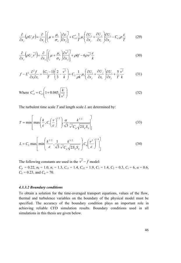
46

T

CxU

x

U

xU

TC

xxU

x j

i

i

j

j

it

j

t

jj

j

2*1

1

(29)

k

vkfx

v

xvU

x jk

t

jj

j

2

22 6

(30)

k

v

Tx

U

x

U

x

U

kC

k

v

T

C

xx

fLf

j

i

i

j

j

it

ii

2

2

21

22 51

3

21

(31)

Where

21*1 045.01

v

kCC (32)

The turbulent time scale T and length scale L are determined by:

ijij

t

SSCv

kvC

kT

23,,maxmin

2

2/32/1

(33)

4/13

2

2/32/3

,23

1,minmax

CSSCv

kkCL

ijij

L (34)

The following constants are used in the fv 2 model:

Cµ = 0.22, σk = 1.0, σε = 1.3, Cε1 = 1.4, Cε2 = 1.9, C1 = 1.4, C2 = 0.3, Ct = 6, α = 0.6, CL = 0.23, and Cη = 70. 4.3.3.2 Boundary conditions

To obtain a solution for the time-averaged transport equations, values of the flow, thermal and turbulence variables on the boundary of the physical model must be specified. The accuracy of the boundary condition plays an important role in achieving reliable CFD simulation results. Boundary conditions used in all simulations in this thesis are given below.

47

At inlet, a uniform temperature was specified; velocity inlet boundary conditions were used which define the flow velocity and all relevant scalar properties. Profiles of the velocity and the corresponding turbulence quantities are provided based on the

measured velocities and the turbulence intensities. Profiles of k, ε, ω or 2v required by different turbulent models are determined by the following formula (ANSYS Fluent, 2010):

25.1 uinin TUk (35)

lkC inin /2/34/3 (36)

lCkinin4/12/1 / (37)

22uinTUv (38)

where, Tu is the turbulence intensity at inlet, and l is a length scale given by l = 0.07Dh, Dh is the hydraulic diameter at the jet discharged section. At exhaust, the pressure outlet boundary condition is used. Flow exits the computational domain at fixed static pressure gauge that is assumed to be zero. All walls are applied with non-slip conditions, and this implies that velocity components on the walls are equal to the velocities of the walls that are zero. The surrounding walls are imposed with fixed temperatures in the validation studies, and specified with constant heat fluxes in the parametric studies. Internal heat sources are imposed with constant heat fluxes in all studies. Radiation effects are accounted by using the DO model. This model solves the radiative transfer equation for a finite number of discrete solid angles, each associated with a vector diction fixed in the global Cartesian system; for more details see ANSYS Fluent (2010). 4.3.3.3 Near-wall treatments

Turbulent flows are significantly affected by the presence of the walls and these flows have complex structures. Adjacent to the walls, mean velocities are rapidly decreased to zero through the no-slip conditions of the walls, and fluctuations both parallel and normal to the walls are damped out by the viscosity and kinematic blocking, consequently resulting in steep velocity gradients and vigorous transports of

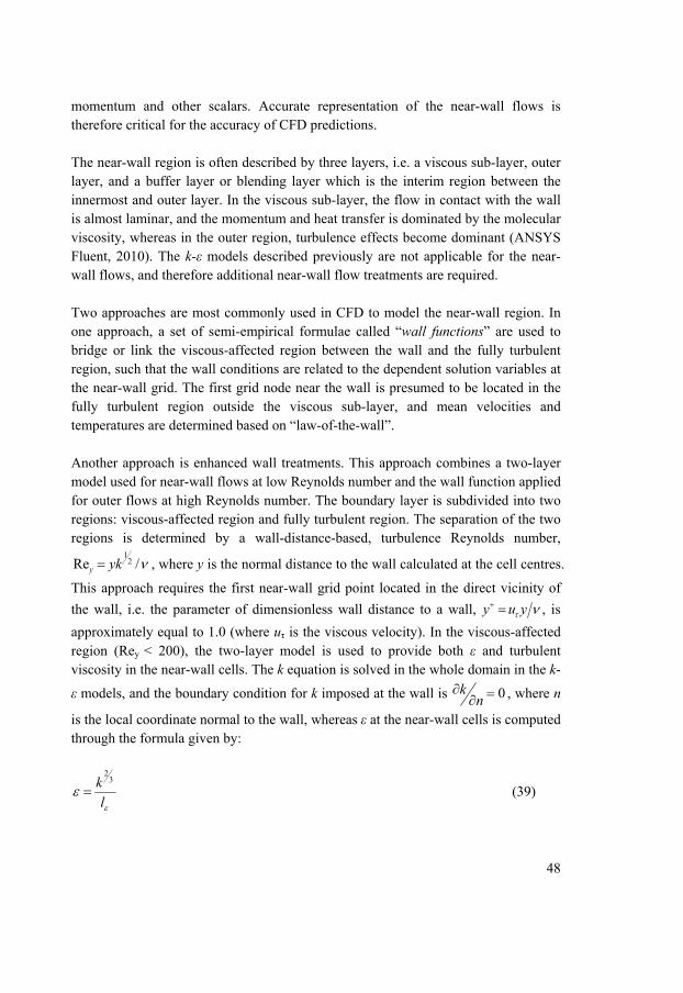
48

momentum and other scalars. Accurate representation of the near-wall flows is therefore critical for the accuracy of CFD predictions. The near-wall region is often described by three layers, i.e. a viscous sub-layer, outer layer, and a buffer layer or blending layer which is the interim region between the innermost and outer layer. In the viscous sub-layer, the flow in contact with the wall is almost laminar, and the momentum and heat transfer is dominated by the molecular viscosity, whereas in the outer region, turbulence effects become dominant (ANSYS Fluent, 2010). The k-ε models described previously are not applicable for the near-wall flows, and therefore additional near-wall flow treatments are required. Two approaches are most commonly used in CFD to model the near-wall region. In one approach, a set of semi-empirical formulae called “wall functions” are used to bridge or link the viscous-affected region between the wall and the fully turbulent region, such that the wall conditions are related to the dependent solution variables at the near-wall grid. The first grid node near the wall is presumed to be located in the fully turbulent region outside the viscous sub-layer, and mean velocities and temperatures are determined based on “law-of-the-wall”. Another approach is enhanced wall treatments. This approach combines a two-layer model used for near-wall flows at low Reynolds number and the wall function applied for outer flows at high Reynolds number. The boundary layer is subdivided into two regions: viscous-affected region and fully turbulent region. The separation of the two regions is determined by a wall-distance-based, turbulence Reynolds number,

/Re 21

yky , where y is the normal distance to the wall calculated at the cell centres.

This approach requires the first near-wall grid point located in the direct vicinity of

the wall, i.e. the parameter of dimensionless wall distance to a wall, yuy , is

approximately equal to 1.0 (where uτ is the viscous velocity). In the viscous-affected region (Rey < 200), the two-layer model is used to provide both ε and turbulent viscosity in the near-wall cells. The k equation is solved in the whole domain in the k-

ε models, and the boundary condition for k imposed at the wall is 0

nk , where n

is the local coordinate normal to the wall, whereas ε at the near-wall cells is computed through the formula given by:

l

k 32

(39)

49

where lε is a turbulent length scale. The formulation for the turbulent viscosity in the two-layer model contains two parts, given by:

subtouttt ,, 1 (40)

where μt,sub and μt,out are the turbulent viscosity in the near-wall region and outer region (computed with k-ε models), and λε is a blending function blending μt,sub and μt,out, which is equal to unity away from walls and zero in the vicinity of the walls. μt,sub in the near-wall region is given by:

klCsubt , (41)

where C is the model constant used in k-ε models. In this thesis, y+ of the first near-wall grid node is less than 1.0 in most of the computational domain. Enhanced wall treatment is used with k-ε turbulence models,

while no-additional near-wall treatments are used with the SST k-ω and fv 2

models, as the viscous sub-layer could be resolved by the turbulence model itself. ω

and ε at the wall-adjacent cells in the SST k-ω and fv 2 model is computed though

Equation (42) and (43), respectively:

2*u

w (42)

where

/

21

41

*

w

kUCu and 2

6

yi

22

pyk

v (43)

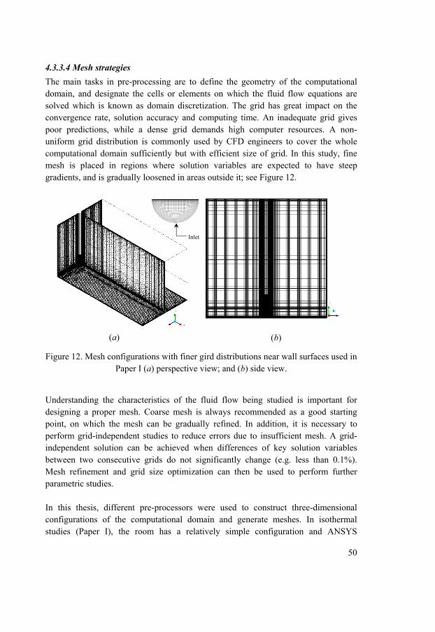
50

4.3.3.4 Mesh strategies

The main tasks in pre-processing are to define the geometry of the computational domain, and designate the cells or elements on which the fluid flow equations are solved which is known as domain discretization. The grid has great impact on the convergence rate, solution accuracy and computing time. An inadequate grid gives poor predictions, while a dense grid demands high computer resources. A non-uniform grid distribution is commonly used by CFD engineers to cover the whole computational domain sufficiently but with efficient size of grid. In this study, fine mesh is placed in regions where solution variables are expected to have steep gradients, and is gradually loosened in areas outside it; see Figure 12.

Figure 12. Mesh configurations with finer gird distributions near wall surfaces used in Paper I (a) perspective view; and (b) side view.

Understanding the characteristics of the fluid flow being studied is important for designing a proper mesh. Coarse mesh is always recommended as a good starting point, on which the mesh can be gradually refined. In addition, it is necessary to perform grid-independent studies to reduce errors due to insufficient mesh. A grid-independent solution can be achieved when differences of key solution variables between two consecutive grids do not significantly change (e.g. less than 0.1%). Mesh refinement and grid size optimization can then be used to perform further parametric studies. In this thesis, different pre-processors were used to construct three-dimensional configurations of the computational domain and generate meshes. In isothermal studies (Paper I), the room has a relatively simple configuration and ANSYS

Inlet

(a) (b)

51

Workbench 13.0 was used. In non-isothermal studies (Paper II, III, IV and V), the presence of different internal heat sources makes the configuration of the domain complex, and Airpak 3.0.16 is chosen due to its simplicity for handling such features. Non-conformal mesh strategy provided by Airpak 3.0.16 was adopted to reduce the size of the total mesh by reducing the grid projections from the air supply inlet and heat sources throughout the whole domain. The grid is non-conformal at interfaces where two sub-domains meet; see Figure 13.

Figure 13. Mesh configurations used for the validation study (Paper II and III) in (a) the whole domain; and (b) in vertical middle plane.

4.3.3.5 Numerical aspects

Closing the governing equations by numerical techniques involves converting the differential equations into algebraic equations, and solving the equations using an iterative method. Several aspects are associated with the solution procedure, such as numerical methods, discretization schemes, pressure-velocity coupling algorithms and convergence criteria, and these are of importance to ensure stability of convergences as well as accuracy of the converged solutions. The numerical Finite Volume Method (FVM) approach is used to perform discretization in all cases in this study. The FVM is based on subdividing the solution domain into a finite number of small control volumes, and solution variables are located at the centroid of each volume. By integrating the partial differential

(a) (b)

52

equations of fluid flow over all the volumes, conservation of relevant properties for each finite size volume is satisfied. In the second step, key terms in the integrated equations representing flow transport phenomena such as convection, diffusion and sources, are substituted by a variety of finite-difference-type approximations resulting in a set of algebraic equations. These equations are not only complex and nonlinear, but also strongly coupled with each other. Simultaneously solving them requires an iterative process. Discretization schemes are an important part of the FVM, which determines how well the resulting algebraic equations represent the true partial differential equations. Discretization error is considered a major source of numerical error. A proper discretization scheme has to be selected in order to get physically realistic results, and such a scheme should possess the fundamental properties of conservativeness, boundedness and transportiveness. First-order schemes have all three of these properties; they are easily implemented and could result in stable calculation. However, they are very diffusive in that gradients of the properties in a flow field tend to be smeared out by “false diffusion”. An upwind scheme with a higher order of accuracy (e.g. second-order upwind scheme) can be used to improve accuracy of the prediction. The second-order upwind scheme determines the value of the cell surface based on values in two upstream notes instead of one upstream note used in the first-order schemes, and hence it is more accurate than the first-order upwind scheme. In this thesis work, the second-order upwind scheme was utilized. Transformations of the differential equations to the algebraic equations can be made for all variables except for pressure because there is no independent pressure equation. To close these derived convection-diffusion equations, pressure needs to be solved as pressure gradients appear in the momentum equations. For incompressible flows, pressure fields can be determined by coupling pressure with the continuity and momentum equations through the so-called pressure-velocity algorithms. The most commonly used algorithm in finite volume codes is the Semi-Implicit Method for Pressure-Linked Equations (SIMPLE), which was also chosen in this work. Residuals are one of the most important indicators for ensuring convergence of the iterative process, which measures the extent of the overall conservation of properties in a converged solution. The iterative process is repeated until the residuals meet specified convergence criteria or no longer change with further iterations. Generally residuals are required to be sufficiently low in order to achieve a high accuracy of the results. The convergence speed and solution stability is controlled by a variety of relaxation factors. By applying a relaxation function with factor, α, on any arbitrary variable ϕ between iteration i and i-1, the new value of ϕ at ith iteration can be

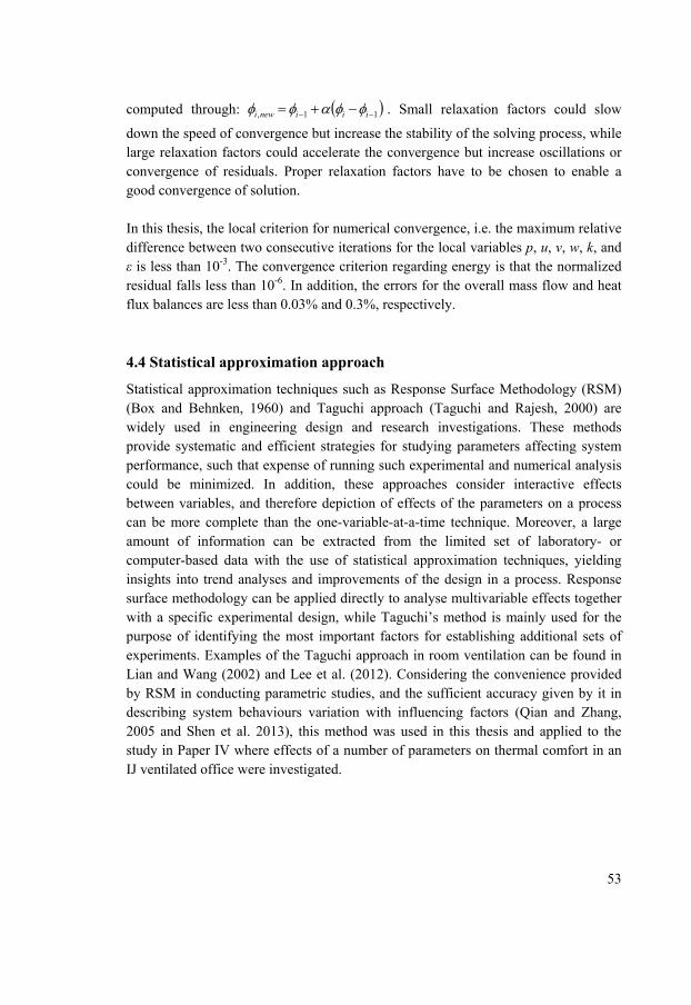
53

computed through: 11, iiinewi . Small relaxation factors could slow

down the speed of convergence but increase the stability of the solving process, while large relaxation factors could accelerate the convergence but increase oscillations or convergence of residuals. Proper relaxation factors have to be chosen to enable a good convergence of solution. In this thesis, the local criterion for numerical convergence, i.e. the maximum relative difference between two consecutive iterations for the local variables p, u, v, w, k, and ε is less than 10-3. The convergence criterion regarding energy is that the normalized residual falls less than 10-6. In addition, the errors for the overall mass flow and heat flux balances are less than 0.03% and 0.3%, respectively.

4.4 Statistical approximation approach

Statistical approximation techniques such as Response Surface Methodology (RSM) (Box and Behnken, 1960) and Taguchi approach (Taguchi and Rajesh, 2000) are widely used in engineering design and research investigations. These methods provide systematic and efficient strategies for studying parameters affecting system performance, such that expense of running such experimental and numerical analysis could be minimized. In addition, these approaches consider interactive effects between variables, and therefore depiction of effects of the parameters on a process can be more complete than the one-variable-at-a-time technique. Moreover, a large amount of information can be extracted from the limited set of laboratory- or computer-based data with the use of statistical approximation techniques, yielding insights into trend analyses and improvements of the design in a process. Response surface methodology can be applied directly to analyse multivariable effects together with a specific experimental design, while Taguchi’s method is mainly used for the purpose of identifying the most important factors for establishing additional sets of experiments. Examples of the Taguchi approach in room ventilation can be found in Lian and Wang (2002) and Lee et al. (2012). Considering the convenience provided by RSM in conducting parametric studies, and the sufficient accuracy given by it in describing system behaviours variation with influencing factors (Qian and Zhang, 2005 and Shen et al. 2013), this method was used in this thesis and applied to the study in Paper IV where effects of a number of parameters on thermal comfort in an IJ ventilated office were investigated.

54

4.4.1 Response surface methodology

Response surface methodology is a collection of mathematical and statistical techniques used for developing an adequate functional relationship between a response of interest and a number of related variables (Khuri and Mukhopadhyay, 2010). The graphical perspective of the relationship expressed by a known mathematical equation has led to the term Response Surface Methodology. By careful design of the experiments, this method is useful in identifying the relative importance of the independent variables along or in combination with a process, as well as determining optimal conditions for a process. The RSM approach has been popularly used in chemical or biochemical fields, while only a few applications in building environments are available; see Ng et al. (2008), Norton et al. (2010) and Shen et al. (2013). The general relationship between response Y and a number of inputs can be described by Equation (44):

exxxfY n )......,,( 21 (44)

Where f is the unknown response function, x1, x2……, xn denote the independent variables, also named as natural variables whose units are physical quantities, n is the number of the independent variables, and the surface represented by f (x1, x2 ······ xn) is called a response surface. e is the error term representing measurement error and other sources of variability that are not accounted for in f. In general, it is assumed that the error is random and has a normal distribution with zero mean and variance. Provided that the response surface is adequately represented by a second-order relation, the estimated response Y for n input variables can be approximated by the following presented function:

eXXXXY ji

n

iij

n

iiii

n

ii i

j

2

110 (45)

Where Y is response variable, Xi is the coded level setting of factor xi which will be explained later, β0 is the model intercept coefficient; βi, βii, and βij are the regression coefficients for the linear, quadratic and interaction terms, and e is the error term. Due to the deterministic feature of the CFD model, the computational error can be negligible in most cases, and therefore there is no need to repeat the simulation to reduce it.

55

An optimization process of RSM consists of four major steps: (a) determining independent variables and their levels; (b) choosing an experimental design for generating data; (c) developing and verifying a model equation which represents the relationship between response and independent variables; (d) generating response surface plots to visualize the established functions and identify optimum points (a set of parameters). 4.4.1.1 Determination of independent variables and their levels

At the first stage, a number of factors that affect a response need to be selected, because it is impossible to identify effects for all parameters. Choice of the levels of these independent variables is another important issue, which is directly related to the success of the optimization. A narrow range of independent parameters could increase the accuracy of the model equation, but reduces the possibility of determination of the optimal point over the studied range (Bas and Boyaci, 2007). Considering the fact that the independent variables differ from one another in terms of units and the tested range, performing regression analysis of the natural variables will become difficult. Instead, the natural variables are scaled to be coded variables ranging from -1 to 1, so that the units and the magnitude of the tested parameters become irrelevant and their effects on responses more even. Transformations of the natural variables to the coded variables are commonly achieved by using the equation stated below:

iLiH

iMii xx

xxX

2 (46)

Where Xi is the coded variable, xi is the natural variable, xiH, xiL represents the high and low level of the ith factor, respectively, and xiM is the average of these. In the coded units, the high, low and mean level of xi becomes XiH = 1, XiL = -1, and XiM = 0.

4.4.1.2 Experimental design

At the second stage, a set of samples or design points that represent different combinations of the levels of the independent variables in a design space is defined through Design of Experiment (DOE) procedure. The design space is an n-dimensional space bounded by the lower and upper limits of each independent parameter, i.e. with a range from -1 to 1. DOE involves selections of the sample points, number of runs and blocks. An appropriate selection of DOE is essential to the

56

accuracy and effectiveness of the experimentation. Sufficient number of samples over the design space ensures adequate representation of the whole space, but this requires conducting massive experiments.

Commonly used second-order RSM designs include the Central Composite Design (CCD) (Box and Wilson, 1951) and Box-Behnken design (BBD) (Box and Behnken, 1960). A CCD is a two-level fractional factorial design expressed by 2k, where k is the number of factors, augmented by the centre points of the design space as well as the points in the centre of the face. Schematic representation of a CCD with three factors (k = 3) each of which has three levels is illustrated in Figure 14(a). As can be seen, a CCD contains a full factorial part of 2k (23 = 8) vertices, 2k (2 × 3 = 6) points at the original of each factor axial and a centre point, resulting in 15 runs in total. The number of experiments, N, required by the CCD is calculated by N = 2k + 2k +C0, where C0 is the number of centre points. A BBD is formed by combining 2k factorial design with incomplete block designs in a particular manner; see Figure 14(b). According to Figure 14(b), the BBD contains three inter-blocking 22 fractional factorial designs, and design points consist of the middle point of each edge and central point of the design space that specifies combinations of the level of each parameter. The total number of runs generated by the BBD is: N = 2k(k-1) + Co. Comparisons between these two experimental design methods can be found in e.g. Ferreira et al. (2007). It was revealed that the BBD is slightly more efficient than the CCD for few factors, but it is much more efficient for larger factors such as over 5. Another advantage of BBD is that it does not contain points at vertices of the hypercube, hence this method is useful in avoiding unsatisfactory results due to extreme conditions.

Figure 14. (a) CCD; and (b) BBD for three factors.

(a) (b)

Design space

-1

1

X3

-1 1 X1 -1

1 X

2

-1 1X1 -1

1 X

2

-1

1

X3

X1, X2, X3 (-1, 0, 1)

57

Considering the advantages provided by BBD, this method is chosen in planning computer experiments in Paper IV, where effects of four factors, each with three levels, on the local thermal discomfort of an IJV system were studied. Table 1 gives coded factor levels based on a three-level four-factor BBD design. In Table 1, the set of required runs is separated with dashed lines and arranged in orthogonal blocks, and each (±1, ±1) combination in a row is a full 22 design give in Table 2. Table 1. Coded factor levels for a three-level four-factor BBD. X1 X2 X3 X4 ±1 ±1 0 0

Block 1 0 0 ±1 ±1 0 0 0 0 ±1 0 0 ±1

Block 2 0 ±1 ±1 0 0 0 0 0 ±1 0 ±1 0

Block 3 0 ±1 0 ±1 0 0 0 0

Table 2. 22 factorial design. X1 X2 -1 -1 1 -1 -1 1 1 1

4.4.1.3 Establishment of the response surface model and verification

At the third stage, measurement or simulation results for design points are used as response values to develop regression equations. Minitab 16.1 is statistical software often used for performing experimental design and data analysis, and also employed in Paper IV. Coefficients of response surface models given by Equation (45) are determined by using the least square method which minimizes the sum of the square of the residuals. Residuals are the difference between the observed and fitted value for a response. Establishing a response model follows two steps. Firstly, develop a second-order equation which contains all the independent parameters (full equation) with the least square method; secondly, examine the statistical significance of each coefficient in the quadratic model based on the probability value (P-value) from analysis of variance (ANOVA). Terms with P < 0.05 indicate that their effects are

58

statistically significant at 95% confidence levels, thus ones with P > 0.05 could be removed from the quadratic model without greatly reducing the accuracy of the model. The final equation is established when all terms in the model are statistically significant (i.e. P < 0.05). It is necessary to check the adequacy of the fitted models on presenting the true relationship between the response and independent variables. At the first step, it is necessary to examine whether residuals satisfy the normality assumption of the response, i.e. the residuals normally and independently distribute with mean zero and variance (Bradley, 2007). This assumption is confirmed provided that residuals approximately follow a straight line. After that, the significance of the regression models is evaluated by the results from ANOVA. P < 0.05 indicates that the relationship between responses and independent variables exists. Lastly, the quality fit of the regression equation is assessed based on the coefficient of determination (R2), i.e. larger R2 implies that more experimental data is explained by the model and hence the model has higher accuracy. In Paper IV, all established response models have P-values smaller than 0.05 and R2 values greater than 98%, indicating that the models are statistically significant and fit the CFD predicted data quite well. 4.4.1.4 Graphical presentation of the response surface model and optimization

The established relationship between the response and independent variables can be visualized through a 3D response surface plot and its corresponding 2D contour plot. These plots are useful for presenting the shape of the response surface and determining optimum points of the response (i.e. maximum or minimum) throughout the design space. In Paper IV, identification of the optimum conditions for minimum local thermal discomfort was not the focus, but instead a range of the parameters studied for providing a good comfort was determined.

59

5. RESULTS AND DISCUSSION

In this chapter some of the results from the appended papers are presented in accordance with the research process stated in the introduction. 5.1 CFD validation results

5.1.1 Isothermal case

The CFD program with RNG k-ε and SST k-ω models was used to predict flow behaviours of an isothermal impinging jet in a room (Paper I), and predicted contour plots of the velocity magnitude in the vertical middle plane are shown in Figure 15. As can be seen, the RNG k-ε model slightly over-predicts diffusion of the jet compared to the SST k-ω model, yielding a thicker wall jet along the floor especially in the beginning of the wall jet. Consequently, the RNG k-ε model under-predicts velocities in the lower part of the wall jet while over-predicting it at higher regions at the nearest compared location of x = 0.3 m (see Figure 16). The SST k-ω model, however, seems to capture the velocity profile satisfactorily. As it moves further, i.e. at x = 1.0 m, both turbulence models perform similarly and somewhat under-estimate velocities at locations above the inner region where the velocity of the jet reaches its maximum value. The discrepancy might be explained partly by the over-predicted local maximum velocity and partly by instabilities in the flow causing variations of the wall jet profile, which could not be captured by steady state simulations, as addressed by Cehlin and Moshfegh (2010). In addition, some experimental uncertainties in measuring flows with high turbulence intensities and reversed flows could also contribute to some of the discrepancies.

Figure 15. Contour plots of velocities in the middle plane of the room predicted by

(a) RNG k-ε; and (b) SST k-ω.

Inlet

(a) RNG k-ε (b) SST k-ω

60

Figure 16. Comparisons of non-dimensional velocity profiles at different locations

along the centreline of the floor, i.e. U/Umax – y/dh, where Umax is the local maximum velocity, y is the height above the floor, and dh is the hydraulic diameter which is

equal to 0.1265 m. The compared locations are shown in Figure 9b. As for the decays of maximum velocities and normal spreading rate of the jet along the floor, both turbulence models are capable of capturing these trends when compared with measurements, particularly for decays of maximum velocities; see Figure 17. However, jet thicknesses predicted by the two turbulence models are somewhat smaller than those in experimental findings due to the over-predicted maximum velocity. Since the RNG k-ε model predicts a greater initial thickness than the SST k-ω model, it consequently gives a thicker jet in the direction perpendicular to the floor on the whole, as can be seen from Figure 17(b). Again, the discrepancy shown in Figure 17(b) could be related to difficulties in capturing the unsteadiness of the wall jet by both CFD and measurements.

Figure 17. Comparisons of (a) decays of maximum velocities; and (b) the normal

spreading rate of jet along the centreline of the floor (y0.5 is the height of U = 0.5Umax, and dh = 0.1265 m).

0

0.1

0.2

0.3

0.4

0.5

0.6

0.7

0.8

0 0.2 0.4 0.6 0.8 1 1.2

y/d

h

U/Umax, at x=0.3 m

Experiment

RNG k-ε

SST k-ω

0

0.1

0.2

0.3

0.4

0.5

0.6

0.7

0.8

0.9

0 0.2 0.4 0.6 0.8 1 1.2

y/d

h

U/Umax, at x=1.0 m

Experiment

RNG k-ε

SST k-ω

(a) (b)

0

0.1

0.2

0.3

0.4

0.5

0.6

0.7

0 2 4 6 8 10

y 0.5

/dh

x/dh

Experiment

RNG k-ε

SST k-ω

0

0.1

0.2

0.3

0.4

0.5

0.6

0.7

0.8

0.9

1

0 2 4 6 8 10

Um

ax/U

in

x/dh

Experiment

RNG k-ε

SST k-ω

61

5.1.2 Non-isothermal case

Paper II compared performance of three k-ε models on predicting velocity and temperature distributions of an impinging jet in an office environment. Although the RNG k-ε model was found to give the best performance, simulation results are not as good when compared with measurements, which suggests other turbulence models

need to be considered. Two more turbulence models, i.e. SST k-ω and fv 2 are also

applied in this research; see Paper III. Figure 18 shows that velocity and temperature profiles predicted by the RNG k-ε

model are significantly improved with the fv 2 model, but slightly improved by the

SST k-ω model, particularly in a region close to jet impingement, i.e. at x = 0.3 m. In essence, the difference is assumed to be related to the amount of turbulent kinetic energy, k, predicted in the vicinity of the stagnation region by each turbulence model. A smaller value of k results in more conserved momentum of the supplied air, while excessive k leads to faster decaying of the supplied momentum hence more rapid mixing with surrounding air (Chen, 1995). Therefore, a more conserved jet results in greater velocities near the floor, and consequently higher air temperatures due to increased heat transfer. As the jet moves further over the floor, i.e. x = 1.0 m, all turbulence models are capable of reproducing the velocity and temperature profiles

quite satisfactorily as the flow features become relatively stable. Still, the fv 2

model shows the best performance and this is also valid for various zones in the room, according to results presented in Paper III.

In addition, results from the fv 2 model are used to provide qualitative illustrations

of the impinging flow which could not be revealed from the experimental data obtained in this study. Figure 19 shows vector plots of the impinging jet flow field. As can be seen, there are several flow mechanisms involved in this type of flow. One notable feature is flow recirculation generated by jet impingement, appearing in the lower left corner in Figure 19. Close to this region the flow patterns are significantly affected by the corner. After impingement, the flow reattaches to the floor and starts to form a wall jet, and this process is accompanied by strong streamline curvature. The wall jet along the floor is fed by the free stream jet and compacts to a thin layer, thus the flow is forced to pass a small area with great momentum consequently leading to a strong flow acceleration (Bovo, 2009); see Figure 19. After that, the wall jet begins to decelerate along the floor. To provide more solid findings on impinging jet flow features as well as precise results for CFD validations, it is suggested that advanced measuring techniques need to be used in this part of the flow.

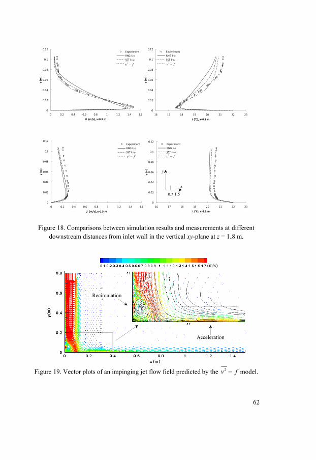
Figuredo

Figure 1

0

0.02

0.04

0.06

0.08

0.1

0.12

0

y (m

)

0

0.02

0.04

0.06

0.08

0.1

0.12

0

y (m

)

e 18. Compaownstream d

19. Vector p

0.2 0.4 0

0.2 0.4 0

arisons betwdistances fro

plots of an i

.6 0.8 1

U (m/s), x=0.3 m

0.6 0.8 1

U (m/s), x=1.5 m

Recirculat

ween simulaom inlet wa

impinging je

1.2 1.4 1.6

Experiment

RNG k‐ε

SST k‐ω

1.2 1.4 1.6

Experiment

RNG k‐ε

SST k‐ω

tion

fv 2

fv 2

ation resultsall in the ver

et flow field

0

0.02

0.04

0.06

0.08

0.1

0.12

16 17

y (m

)

Exper

RNG

SST k

6

0

0.02

0.04

0.06

0.08

0.1

0.12

16 17

y (m

)Expe

RNG

SST k

0.3

y

v 2

v 2

s and measurtical xy-pla

d predicted

18 19

t (°C), x=

riment

k‐ε

k‐ω

18 19

t (°C), x=

riment

k‐ε

k‐ω

3 1.5

x

Ac

f

f

urements at ane at z = 1.

by the v 2

20 21

=0.3 m

20 21

=1.5 m

cceleration

(m/s)

62

different .8 m.

f model.

22 23

22 23

63

5.2 Parametric studies

In this thesis, three sets of parametric studies were carried out to investigate different scenarios and the most important findings from these are presented below. 5.2.1 Parametric study (one-factor-at-a-time): part one

The validated CFD program with the SST k-ω model was used further to investigate influences of a number of parameters on the flow behaviour of an impinging jet under isothermal conditions, see Paper I. One parameter considered in this paper is configurations of the IJ supply device (see Figure 20), which was found to have the most significant effect on flow behaviours (see Figure 21). In this case four duct geometries were investigated with the same cross-sectional area.

Figure 20. Sketch for the shapes of impinging jet supply devices with the same area of 0.01667 m2: (a) semi-elliptic; (b) square; (c) rectangular 1 with aspect ratio, AR,

defined by a/b, of 2.5; and (d) rectangular 2 with AR = 10.

Based on Figure 21(a) and (b), it can be seen that the jet discharged from the semi-elliptic air supply device tends to distribute the flow radially over the floor, while the one from the square duct appears to spread approximately equally in the longitudinal and lateral directions. For flows issued from rectangular supply devices, the wall jets tend to penetrate more forward and this is especially apparent in the case with AR = 10; see Figure 21(c) and (d). The difference in airflow patterns and jet penetration distances might be explained by the fact that when lateral movements of air are weak, a jet is more directed towards the longitudinal direction in accordance with the principle of mass conservation. The rectangular air supply device with larger aspect ratio (e.g. AR = 10) is therefore more suitable for industrial premises than others with

(a) (b) (c)

(d)

64

comparable AR, as it is able to deliver fresh air over longer distances in the space being ventilated.

Figure 21. Contour plots of the iso-velocity with 0.25 m/s for different IJ air supply devices: (a) semi-elliptic; (b) square; (c) rectangular with AR = 2.5; and (d)

rectangular with AR = 10. 5.2.2 Parametric study (one-factor-at-a-time): part two

Since a cooled ceiling (CC) is often integrated with a ventilation system to cope with a high heat load in a room, the effects of CC, heat sources (including locations, type and heat load), and the type of air supply systems, on the thermal patterns and comfort levels needs to be investigated, in order to understand potential adverse impacts on the performance of ventilation systems. Parametric studies of part two

were planned for this purpose and carried out by using the validated fv 2 model for

an office environment; see Paper III. Table 3 lists relevant case studies with IJV presented in this section, where Case 1 considers a small heat load in the room while Case 2 considers extreme conditions. The combination effects of CC, heated window and IJV were found to result in a large air circulation in the room, as can be noted from Figure 22. Beneath the ceiling, air moves in a general tendency towards the air inlet wall, driven by buoyancy forces

(a) (b)

(c) (d)

x

y

z

65

from the thermal plume close to the window. Due to buoyancy effects from internal heat sources (e.g. occupant), the flow tends to be directed towards the opposite side of the room; see Figure 22(b). Close to the corner between the inlet and rear walls, a stream of downward flow is formed which is noticeable in Figure 22(a) and (c). This downward flow merges with primary flows in the lower part of the room and consequently increases the momentum of the flow penetrating into the room, which leads to a higher velocity at certain positions as well as a longer flow projection to the room. Table 3. Major parameters used in case studies. Case No. Heat load

of floor area (W/m2)

Heat load Ts (°C)

qv (m3/s)

CC cooling load (W)

CC/total cooling load Total IHLa

(W) EHLFb (W)

EHLWc (W)

1 17 257 0 0 17 0.023 0 0 2 65 257 200 526 17 0.023 -790 0.8 a IHL: internal heat load. b EHLF: external heat load imposed on the floor. c EHLW: external heat load imposed on the window.

Figure 22. Computed streamlines for Case 2: (a) perspective view; (b) top view; and

(c) front view.

(a) (c)

(b)

The contemperatgradient effects pgradient temperatmaximum AlthoughtemperatCase 1 bmarked increase

Figure

Figure 2

nsequent efture distribin Case 2

provoked byis observ

ture differem allowabl

h Case 1 anture of 17 because of in Figure d to 20% in

23. Temper

24. Predicte

(a

ffect on theutions for tis greatly r

y the large aved, local ence betwee value, acc

nd 2 have t°C, the PDthe downw24. The m

n Case 2.

rature distri

ed PD distrib(

a)

(a)

Occ

ermal fieldsthe two casreduced as air circulatithermal co

een 0.1 andcording to IS

he same suD values in ward flow, wmaximum va

ibutions at t

butions at tha) Case 1; a

cupant

s can be seses are comcompared t

ion. In Caseomfort is sd 1.1 m leSO 7730:20

upply air floCase 2 are

which is espalue of PD

the mid-sect

he surface 0and (b) Case

(

een in Figumpared: theto that in Ce 1, althougstill acceptevels (abou005 (ISO 77

ow rate of 0e generally pecially not

D in Case

tion: (a) Ca

0.1 m abovee 2.

(b)

(b)

Zon

ure 23 whee vertical teCase 1, due h a sharp tetable as thut 2°C) is 730, 2005).

0.023 m3/s ahigher thanticeable in 1 is 10% w

ase 1; and (b

e the floor (t

Mid-secti z = 1.8 m

ne A

66

ere vertical emperature to mixing emperature he vertical below the

and supply n those for Zone A as while it is

b) Case 2.

top view):

tion at m

67

5.2.3 Parametric study (based on response surface methodology): part three

Parameters related to air supply devices and supply conditions of IJV were

investigated further with the use of the fv 2 model, together with the response

surface methodology which considers simultaneous effect of changes in two or more parameters (design variable) on results (response); see Paper IV. The responses are focused on draught discomforts and vertical temperature differences in an occupied space for an office environment. Figure 25 shows details of air supply devices considered in Paper IV; Table 4 lists the range of independent parameters considered as a possible requirement for providing thermal comfort by IJV. Twenty-five CFD simulations have been performed based on a matrix designed by the three-level, four-factor Box-Behnken method. For details of the design matrix as well as energy balance information, see Paper IV.

Figure 25. Sketch for the three shapes of impinging jet supplies with the same area of

0.01667 m2: (a) rectangular shape; (b) semi-elliptic shape; and (c) square shape. Table 4. Levels of the independent variables (design variables).

Independent variables (unit) Low level (-1) Middle level (0) High level (1)

Shape of air supply device1(m) 0.1240 (rectangular) 0.1265 (semi-elliptic) 0.1290 (square) Discharge height H (m) 0.4 0.8 1.2 Supply airflow rate Q (m3/s) 0.020 0.025 0.030 Supply temperature Ts (°C) 14 16 18

1The shape of air supply device is represented by Dh.

Results show that PD assessed at the 0.1 m level is more sensitive to different levels of design variables than temperature gradients. The square air supply device was found to generate lower draught discomforts than the rectangular one at the same discharge height and same supply conditions. The difference can be explained by

(a) (b) (c)

68

flow patterns presented in Figure 26. For more information about Figure 26 see Paper IV. Figure 26(a-c) shows that at a low discharge height, i.e. H = 0.4 m, flow fields in the vicinity of the supply device are significantly influenced by the shape of the air supply device because of the footprint from impinging jet. Flow patterns for the three shapes of supply devices (i.e. rectangular, semi-elliptic and square) are found to be similar to those presented in Figure 21, and therefore the difference can be explained by the same spreading mechanics as described in section 5.2.1. However, flow features near the floor are not closely related to shapes of air supply device at higher discharge heights H, as can be noted from Figure 26(d-f). This is because more entrainment causes the jet to be rounder before it strikes the floor with elevated H. Overall, the square air supply device leads to the shortest penetration distance in the occupied zone and therefore gives the lowest PD values. Moreover, the jet flows near the floor with all three air supply devices are found to be rather thin, i.e. flows in the room are not thicker than 0.1 m.

Figure 26. Contour plots of iso-velocity with 0.25 m/s for discharge height H = 0.4 m: (a) rectangular shape; (b) semi-elliptic shape; and (c) square shape; for H = 1.2 m: (d)

rectangular shape; (e) semi-elliptic shape; and (f) square shape.

(a) (c)

(d) (e) (f)

Transparency plane at y = 0.1 m

Flow below 0.1 m plane

Flow above 0.1 m plane

Examined plane for local thermal discomfort

(b)

69

With the use of RSM, correlations for draught (PD) and temperature stratification (ΔT1.7-0.1 and ΔT1.1-0.1) discomfort were developed and presented as in Equations (47)-

(49), where hDX , HX , QX , and

sTX are the normalized design parameters of the

shape of supply device, the discharge height, the supply airflow rate and the supply air temperature, respectively. Based on Equations (47)-(49), it can be noted that the supply airflow rate has the greatest impact on PD, and the shape of device has a moderate effect. ΔT1.7-0.1 and ΔT1.1-0.1 are most significantly influenced by the supply air temperature.

QDD

TQHD

XXXXXXXPD

hh

sh

8357.09682.26082.12208.47540.1089.26783.14

2 (47)

ssh

sh

TQTHQDH

TQHD

XXXXXXXXXXXT

05623.003751.004214.004628.0558.004823.012591.00139.078857.2

21.07.1 (48)

sh TQHD XXXXT 40019.011267.012096.002172.095025.11.01.1 (49)

5.3 Ventilation performance comparison

In Paper V, performance of the impinging jet supply device (IJSD) was compared with other air supply devices, i.e. mixing supply device (MSD), wall confluent jets supply device (WCJSD), and displacement supply device (DSD), under certain conditions for an office environment, with a focus on thermal comfort, ventilation efficiency as well as energy-saving potential. Figure 27 shows room airflow patterns from the four studied devices, represented by iso-velocity of 0.25 m/s together with the temperature contour plots. Areas shown in Figure 27 were regions where velocities of the flow were equal to 0.25 m/s, and the colours represented air temperatures. Figure 27 was for a case with a heat load of 17 W/m2 and all devices were supplied with the same air-flow rate of 0.025 m3/s and the same air temperature of 16 °C. As can be seen, the area with the

velocity of 0.25 m/s and flow temperatures of the air penetrating into the room with the IJSD were in between that from the MSD and DSD, because of the moderate installation height of the IJSD, supply momentum, and entrainment involved in the impinging jet ventilation process. Discussions on airflow patterns from other studied air supply devices can be found in Paper V.

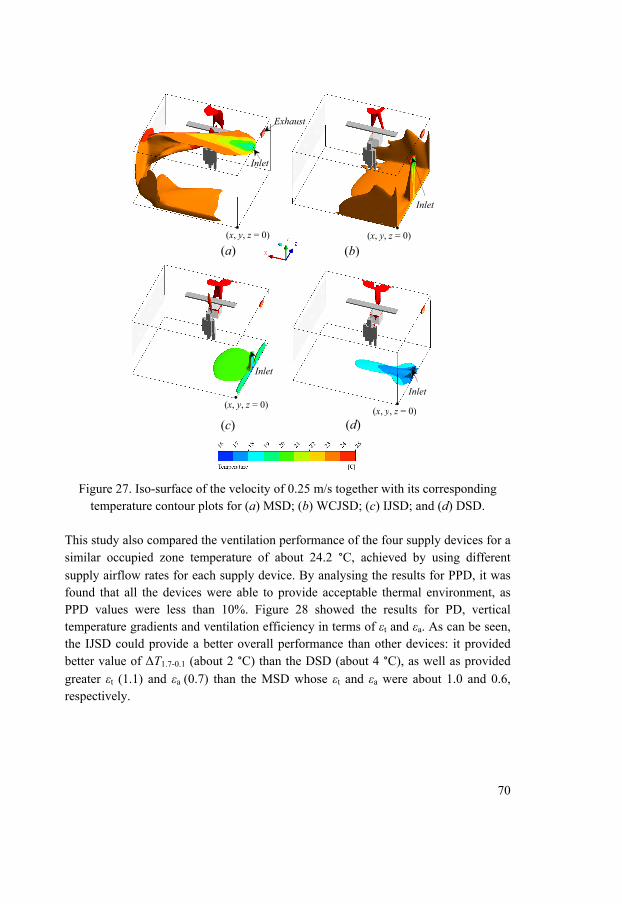
70

Figure 27. Iso-surface of the velocity of 0.25 m/s together with its corresponding

temperature contour plots for (a) MSD; (b) WCJSD; (c) IJSD; and (d) DSD. This study also compared the ventilation performance of the four supply devices for a similar occupied zone temperature of about 24.2 °C, achieved by using different

supply airflow rates for each supply device. By analysing the results for PPD, it was found that all the devices were able to provide acceptable thermal environment, as PPD values were less than 10%. Figure 28 showed the results for PD, vertical temperature gradients and ventilation efficiency in terms of εt and εa. As can be seen, the IJSD could provide a better overall performance than other devices: it provided better value of ΔT1.7-0.1 (about 2 °C) than the DSD (about 4 °C), as well as provided

greater εt (1.1) and εa (0.7) than the MSD whose εt and εa were about 1.0 and 0.6, respectively.

(a) (b) (x, y, z = 0) (x, y, z = 0)

Inlet

Exhaust

Inlet

(d) (x, y, z = 0)

Inlet

(c)

(x, y, z = 0)

Inlet

71

Figure 28. Performance comparisons of the four air supply devices at the same occupied zone temperature achieved by different supply air flow rates.

Energy-saving potential was addressed based on the airflow rates required for each system for obtaining the equivalent occupied zone temperature. The IJSD required slightly higher airflow rate (1.1 times) and fan power (1.3 times) than the DSD, but it was more energy efficient than the MSD and the WCJSD which required 1.2 times higher airflow rate and 1.7 times higher fan power, based on the relations between the flow rate, Q, pressure difference, Δp, and the fan power, E, i.e. 32, QEQp

(Karimipanah et al. 2008). The airflow rate required by the IJSD was 0.023 m3/s.Although the DSD showed superior performance to all other supply devices in terms of ventilation efficiency and energy saving, it seemed to have difficulties in providing acceptable vertical temperature gradient between the ankle and head levels for a standing person. This study showed that the IJSD could provide a better overall performance than other examined devices. It is worth mentioning that this conclusion was limited to specific room conditions and certain types of air supply devices that have been considered in this study. To make a general conclusion, a complete study concerning various kinds of situations and other types of air supply devices is needed.

0.0

0.2

0.4

0.6

0.8

1.0

1.2

1.4

1.6

ε t

MSD

WCJSD

IJSD

DSD

0

0.1

0.2

0.3

0.4

0.5

0.6

0.7

0.8

0.9

1

ε a

MSD

WCJSD

IJSD

DSD

0.0

5.0

10.0

15.0

20.0

25.0

30.0

35.0

PD a

t 0.1

m (%

) MSD

WCJSD

IJSD

DSD

0

0.3

0.6

0.9

1.2

1.5

1.8

16 18 20 22 24 26

Heig

ht (m

)

T (°C)

MSDWCJSDIJSDDSD

73

6. CONCLUSIONS

This thesis presents a recently developed ventilation concept called impinging jet ventilation that has a potential for creating a good indoor environment while using energy efficiently. The aim of this thesis is to investigate the airflow and temperature fields, thermal comfort as well as ventilation effectiveness with respect to heat removal effectiveness and air exchange efficiency of the impinging jet ventilation system for an office environment, by using CFD simulations supported by field measurements. This project has been carried out following a research process consisting of three parts: a validation study, a parametric study and a comparison study. The conclusions from each part are given below.

6.1 Validation study

The accuracy of the predicted velocity and temperature distributions in a room with the IJ supply device is highly dependent on the performance of turbulence models to account for the impingement effects. Although the RNG model gives the best agreement with measurements of the three k-ε models

used (Paper II), the predicted results were further improved by the fv 2

model (greatly) and the SST k-ω models (slightly), as reported in Paper III. The difference is believed to be related to the prediction of the turbulence kinetic energy, which is tuned specially for impinging jet applications in the

fv 2 model.

From results presented on Paper I, both RNG k-ε and SST k-ω models give similar and reasonable predictions of the flow behaviour of an isothermal impinging jet. The SST k-ω model accords slightly better with measured data in regions close to the impingement zone than the RNG k-ε model, which is a crucial zone that influences the spreading of jet inside the room.

The predictions by all turbulence models seem to be improved as the jet moves further away from the impingement region due to reduced complexities of the flow field. Near the stagnation region, the flows present a strong recirculation, curvature and instability, etc., which imposes challenges to the currently used turbulence models and the assumption of a steady state flow.

The uncertainty of measurements is another factor contributing to the discrepancy between CFD simulation and measurement, especially when

74

measuring flows with high turbulence intensities and reversed features. Advanced measuring techniques such as PIV and LDA are highly recommended.

6.2 Parametric study

The results from Paper I show that the geometry of the IJ supply device has the most significant impact on the impinging jet flow field. The rectangular air supply device with the largest aspect ratio of 10 is observed to provide the longest penetration distance into the room, which implies that this shape could be suitable for ventilation of large areas such as industrial premises. The jet discharge height (0.30 – 0.95 m) imposes certain effects on the flow field, but is only noticeable in regions close to air supply devices.

Results reported in Paper III revealed that the interaction effect of cooling ceiling and heat sources with IJV results in complex flow phenomena with notable air circulation zones, the characteristics of which essentially depend on the thermal strengths of heat sources and number of occupants. This effect is found to reduce vertical temperature gradients while increasing draught discomfort near the floor, which needs to be considered when implementing a cooling ceiling for the enhancing cooling capacity of IJV.

As shown in Paper IV, the application of response surface methodology with CFD is a useful method for studying simultaneous effects on changes involving two or more parameters systematically and efficiently. Analysis of the flow field reveals that the low discharge height and the shape of air supply device have major impacts on the flow pattern in the vicinity of the supply device due to the footprint of the impinging jet. In this study, correlations between independent parameters and responses (i.e. PD and vertical temperature gradients) have also been derived, and the supply airflow rate was found to be the most important parameter with regards to draught discomfort due to its greatest coefficient in these correlations.

6.3 Ventilation performance comparison study

Results from Paper V show that the impinging jet device could provide a better overall performance than the other examined air supply devices intended for mixing, wall confluent jets and displacement ventilation, in terms of the overall and local thermal comfort, heat removal effectiveness, air

75

exchange efficiency, and energy-saving potential related to fan power, as it combined positive effects from mixing and displacement ventilation principles.

Since this study is limited to specific room conditions and certain types of air supply devices, conclusions are not applicable to general cases. To conduct a more complete evaluation and derive more general conclusions of these ventilation systems, more studies with a wider scope are needed.

77

7. FUTURE WORK

The studies presented in this thesis could be investigated further to get a complete overview of the impinging jet ventilation system. It would be necessary to refine our understanding of the flow physicals of IJ for room ventilation, as this would be useful for improving the system design as well as for validating CFD methods to attain higher confidence levels. In addition, further studies concerning the effects of parameters such as the IJ supply device location, the inlet area, and the number used, as well as the building environment in which the system is applied, need to be carried out for maximizing system performance and increasing its popularity. A number of suggestions for further work are listed below:

Advanced measuring techniques such as Particle Image Velocimetry could be used to record velocity vectors and demonstrate turbulent flow structures for different regions of impinging jet. Such velocity data is of great importance, not only for revealing the underlying flow mechanisms affecting the ventilation system performance, but also for numerical validation purposes.

Unsteady state CFD simulations with the fv 2 model would be

recommended for studying the instability of the flow as well as its effects on the indoor room environment. It would also be of interest to examine the performance of the Reynolds Stress Model with enhanced wall treatment for predicting the IJ behaviour.

Location of IJ air supply device could be one of the interesting parameters that needs to be investigated. According to Varodompun (2008), an IJV system can be categorized as one of three types: radial, wall (studied in this thesis), and corner IJV. Unlike radial and wall IJV, corner IJV is strongly affected by the side walls. Due to the restricted distribution space in corner IJV (i.e. 90 degree distribution instead of having 360 degree), the jet momentum is more conserved and the velocity is greater than those in radial IJV. However, there is a lack of scientific studies available in the literature on corner IJV performance.

Indoor air quality for IJV is a necessary subject of investigation. The function of IJV for providing good indoor air quality and thermal comfort needs to be assessed in relation to energy performance. The ventilation effectiveness for heat and contaminant removal for IJV can then be further evaluated and compared with values derived for other types of ventilation systems.

78

The performance of IJV in other types of building environments, such as classrooms, conference rooms and industrial premises would be interesting to study. These buildings represent different types of space layout and volume, as well as different levels of heat load. In those studies, different inlet areas, air supply velocities, temperatures and numbers of IJ supply device may be involved in order to remove as much excess heat as possible.

The performance of IJV installations in actual rooms to provide cooling and heating would be desirable. In addition, questionnaires and surveys on occupants’ draught discomfort would also be useful to include in such case studies.

To fully evaluate ventilation performances of IJV and compare it with other ventilation systems, a complete study on the impacts of heat load (including its type, location, load), space configuration, supply airflow rates and temperatures, supply diffuser type, inlet height, cooling and heating modes, etc. would be needed.

79

REFERENCES

Abanto, J., Barrero, D., Reggio, M., & Ozell, B. (2004). Airflow modelling in a computer room. Building and Environment, 39(12), 1393-1402. Abdon, A., & Sundén, B. (2001). Numerical investigation of impingement heat transfer using linear and nonlinear two-equation turbulence models. Numerical Heat Transfer, Part A(40), 563-578. Adrian, R. J. (2005). Twenty years of particle image velocimetry. Experiments in Fluids, 39, 159-169. Allocca, C., Chen, Q., & Glicksman, L. (2003). Design analysis of single-sided natural ventilation. Energy and Buildings, 35(8), 785-795. Ashfort-Frost, S., & Jambunathan, K. (1996). Numerical prediction of semi-confined jet impingement and comparison with experimental data. International Journal for Numerical Methods in Fluids, 23(3), 295-306. ASHRAE (2010). ANSI/ASHRAE Standard 55-2004, Thermal Environmental Conditions for Human Occupancy. American Society of Heating, Refrigerating, and Air-conditioning Engineers, Atlanta. ASHRAE Handbook Fundamentals (2009). American Society of Heating, Refrigerating and Air-Conditioning Engineers, Atlanta. ANSYS Fluent 13.0. (2010). Theory guide. ANSYS Inc. Awbi, H. B. (1989). Application of computational fluid dynamics in room ventilation. Building and Environment, 34 (1), 73-84. Awbi, H. B. (1998). Energy efficient room air distribution. Renewable Energy, 15(1-4), 293-299. Awbi, H. B. (2003). Ventilation of Buildings. Spon Press. Awbi, H. B. (2008). Ventilation system design and performance. London and New York: Taylor & Francis.

80

Bas, D., & Boyaci, I. H. (2007). Modelling and optimization I: Usability of response surface methodology. Journal of Food Engineering, 78(3), 836-845. Behnia, M., Parneix, S., & Durbin, P. A. (1998). Prediction of heat transfer in an axisymmetric turbulent jet impinging on a flat plate. International Journal of Heat and Mass Transfer, 41(12), 1845-1855. Behnia, M., Parneix, S., Shabany, Y., & Durbin, P. A. (1999). Numerical study of turbulent heat transfer in confined and unconfined impinging jets. International Journal of Heat and Fluid Flow, 20(1), 1-9. Box, G. E. P., & Behnken, D. W. (1960). Some new three level designs for the study of quantitative variables. Technometrics, 2(4), 455-475. Box, G. E. P., & Wilson, K. B. (1951). On the experimental attainment of optimum conditions. Journal of the Royal Statistical Society, Series B, 13, 1- 45. Bovo, M., Etemad, S., & Davidson, L. (2009). On the numerical modelling of impinging jet heat transfer. International Symposium on Convective Heat and Mass Transfer in Sustainable Energy, Tunisia. Bradley, N. (2007). The response surface methodology. Master’s thesis, Indiana University of South Bend, South Bend, USA. Brohus, H. (1997). Personal exposure to contaminant sources in ventilated rooms. Doctoral thesis, Alborg University, Alborg, Denmark, ISSN 0902-7953 R9741. Bruun, H. H. (1995). Hot-Wire Anemometry, Principles and Signal Analysis. Oxford University Press, New York. Busch, J. F. (1992). A tale of two populations: thermal comfort in air-conditioned and naturally ventilated offices in Thailand. Energy and Buildings, 18(3/4), 235-249. Buratti, C., Mariani, R., & Moretti, E. (2011). Mean age of air in a naturally ventilated office: Experimental data and simulations. Energy and Buildings, 43(8), 2021-2027. Cao, G. Y., Kurnitski, J. & Mustakallio, P. (2007). Draught risk evaluation in rooms with chilled beams. Proceedings of the ROOMVENT, 101-110, Helsinki, Finland.

81

Cao, G. Y. (2009). Modelling the attached plane jet in a room. Doctoral thesis, Helsinki University of Technology, Espoo, Finland. Cao, G. Y., Sivukari, M., Kurnitski, J., & Ruponen, M. (2010). PIV measurement of the attached plane jet velocity field at a high turbulence intensity level in a room. International Journal of Heat and Fluid Flow, 31(5), 897-908. Cehlin, M., & Moshfegh, B. (2000). Visualization and measurement of air temperature using infrared thermography. Proceedings of the ROOMVENT, Vol. 1, 339-347, Reading, UK. Cehlin, M., Moshfegh, B., & Sandberg, M. (2002). Measurements of air temperatures close to a low-velocity diffuser in displacement ventilation using an infrared camera. Energy and Buildings, 34(7), 687-698. Cehlin, M. (2006). Visualization of airflow, temperature and concentration indoors, whole-field measuring methods and CFD. Doctoral thesis, Royal Institute of Technology, Stockholm, Sweden. Cehlin, M., & Moshfegh, B. (2010). Numerical modelling of a complex diffuser in a room with displacement ventilation. Building and Environment, 45(10), 2240-2252. Charles, K .E. (2003). IRC Research Report RR-162: Fanger’s Thermal Comfort and Draught Models. Institute for Research in Construction, Canada. Chanteloup, V., & Mirade, P. (2009). Computational fluid dynamics (CFD) modelling of local mean age of air distribution in forced-ventilation food plants. Journal of Food Engineering, 90(1), 90-103. Chen, Q. Y. (1995). Comparison of three different k-ε models for indoor airflow computations. Numerical Heat Transfer, Part B: Fundamentals, 28(3), 353-369. Chen, Q. (1996). Prediction of room air motion by Reynolds-Stress models. Building and Environment, 31(3), 233-244. Chen, Q., & Glicksman, L. (2003). System performance evaluation and design guidelines for displacement ventilation, ASHRAE, Atlanta, GA.

82

Chen, Q. Y., & Srebric, J. (2002). A procedure for verification, validation, and reporting of indoor environment CFD analyses. HVAC&R Research, 8(2), 201-216. Chen, Y. L., & Wen, J. (2010). Comparison of sensor systems designed using multizone, zonal, and CFD data for protection of indoor environments. Building and Environment, 45(4), 1061-1071. Chiang, W. H., Wang, C. Y., & Huang, J. S. (2012). Evaluation of cooling ceiling and mechanical ventilation systems on thermal comfort using CFD study in an office for subtropical region. Building and Environment, 48, 113-127. Chung, Y. M., Luo, K. H., & Sandham, N. D. (2002). Numerical study of momentum and heat transfer in unsteady impinging jets. International Journal of Heat and Fluid Flow, 23(5), 592-600. Cooper, D., Jackson, D. C., Launder, B. E., & Liao, G. X. (1993). Impingement jet studies for turbulence model assessment–I. Flow-field experiments. International Journal of Heat Mass Transfer, 36 (10), 2675-2684. Craft, T. J., Graham, L. J. W., & Launder, B. E. (1993). Impinging jet studies for turbulence model assessment–II. An examination of the performance of four turbulence models. International Journal of Heat and Mass Transfer, 36(10), 2685-2697. Dewan, A., Dutta, R., & Srinivasan, B. (2012). Recent trends in computation of turbulent jet impingement heat transfer. Heat Transfer Engineering, 33(4-5), 447-460. Durbin, P. (1991). Near-wall turbulence closure without damping functions. Theoretical and Computational Fluid Dynamics, 3, 1-13.

Durbin, P. A. (1995). Separated Flow Computations with the k-ε- 2v Model. AIAA Journal, 33(4), 659-664. Elvsen, P. A., & Sandberg, M. (2009). Buoyant jet in a ventilated room: Velocity field, temperature field and airflow patterns analysed with three different whole-field methods. Building and Environment, 44(1), 137-145. Etheridge, D., & Sandberg, M. (1996). Building ventilation theory and measurement. John Wiley & Sons, England.

83

Fairweather, M., & Hargrave, G. K. (2002). Experimental investigation of an axisymmetric, impinging turbulent jet. 1. Velocity field. Experiments in Fluids, 33(4), 539-544. Fanger, P. O. (1970). Thermal comfort. Copenhagen: Danish Technical Press. Fanger, P. O., &. Christensen, N. K. (1986). Perception of draught in ventilated spaces. Ergonomics, 29 (2), 215-235. Fanger, P. O., Melikov, A. K., Hanzawa, H., & Ring, J. (1988). Air turbulence and sensation of draught. Energy and Buildings, 12(1), 21-39. Ferreira, S. L. C., Bruns, R. E., Ferreira, H. S., Matos, G. D., David, J. M., Brandao, G. C., da Silva, E. G. P., Portugal, L. A., dos Reis, P. S., Souza, A. S., & dos Santos, W. N. L. (2007). Box-Behnken design: An alternative for the optimization of analytical methods. Analytica Chimica Acta, 597(2), 179-186. Finkelstein, W., Melikov, A. K., Sefker, T., & Langkilde, G. (1996). Laser Doppler measurements of airflow characteristics in rooms with mechanical ventilation. Proceedings of Indoor Air, Nagoya, Japan. Gan, G. H. (2000). Effective depth of fresh air distribution in rooms with single-sided natural ventilation. Energy and Buildings, 31, 65-73. Gauntner, J. W., Livingood, J. N. B., & Hrycak, P. (1970). Survey of literature on flow characteristics of a single turbulent jet impinging on a flat plate, NASA Technical Note (NASA TN D-5652). Grinzato, E., Marinetti, S., & Bison, P. G. (2004). Air tightness monitoring by IR thermography. Proceedings of SPIE - the International Society for Optical Engineering, 5405, 132-143. Goldstein, R. J. (1978). Fluid mechanics measurements. Washington, DC: Taylor & Francis. Gutmark, E., Wolfshtein, M., & Wygnanski, I. (1978). The plane turbulent impinging jet. Journal of Fluid Mechanics, 88(4), 737-756. Hagström, K., Sandberg, E., Koskela, H., & Hautalampi, T. (2000). Classification for the room air conditioning strategies. Building and Environment, 35 (8), 699-707.

84

He, G., Yang, X., & Srebric, J. (2005). Removal of contaminants released from room surfaces by displacement and mixing ventilation: modelling and validation. Indoor air, 15, 367-380. Hollworth, B. R., & Durbin, M. (1992). Impingement cooling of electronics. ASME Journal of Heat Transfer, 114, 607-613. ISO 7730 (2005). Moderate thermal environments - determination of the PMV and PPD indices and specification of the conditions for thermal comfort. International Organization for Standardization, Geneva. Jambunathan, K., Lai, E., Moss, M. A., & Button, B. L. (1992). A review of heat transfer data for single circular jet impingement. International Journal of Heat and Fluid Flow, 13(2), 106-115. Janbakhsh, S., Moshfegh, B., & Ghahremanian, S. (2010). A newly designed supply diffuser for industrial premises. International Journal of Ventilation, 9(1), 59-67. Jiang, X., Zhao. H., & Luo, K. H. (2007). Direct computation of perturbed impinging hot jets. Computers and Fluids, 36, 259-272. Jorgensen, F. E. (2002). How to measure turbulence with hot-wire anemometers - a practical guide, Dantecdynamics: Skovlunde, Denmark. Karimipanah, T. (1996). Turbulent jets in confined spaces. Doctoral thesis, Royal Institute of Technology – Centre for Built Environment, Sweden. Karimipanah, T., & Awbi, H. B. (2002). Theoretical and experimental investigation of impinging jet ventilation and comparison with wall displacement ventilation. Building and Environment, 37(12), 1329-1342. Karimipanah, T., Awbi, H. B., & Moshfegh, B. (2008) The air distribution index as an indicator for energy consumption and performance of ventilation systems. Journal of the Human-Environmental System, 11(2), 77-84. Karimipanah, T., Sandberg, M., & Awbi, H. B. (2000). A comparative study of different air distribution system in a classroom. Proceedings of the ROOMVENT, Reading, UK.

85

Khuri, A. I., & Mukhopadhyay, S. (2010). Response surface methodology, Computational Statistics, 2(2), 128-149. Kinnear, D., Atherton, M., Collins, M., Dokhan, J., & Karayiannis, T. (2006). Colour in visualisation for computational fluid dynamics. Optics and Laser Technology, 38(4-6), 286-291. Knight, K. J., Debus, K. K., Berkoe, J. M., & Dasey, T. J. (2005). Practical application of the LES method to mixing in large indoor spaces. Proceedings of the ASME Fluids Engineering Division, 261, 587-594. Knowles, K. (1996). Computational studies of impinging jet using k-ε turbulence models. International Journal for Numerical Methods in Fluids, 22, 799-810. Knowles, K., & Myszko, M. (1998). Turbulence measurements in radial wall-jets. Experimental Thermal and Fluid Science, 17(1-2), 71-78. Koskela, H., Häggblom, H., Kosonen, R., & Ruponen, M. (2012). Flow pattern and thermal comfort in office environment with active chilled beams. HVAC&R Research, 18(4), 723-736. Lan, L., Wargocki, P., Wyon, D. P., & Lian, Z. (2011). Effects of thermal discomfort in an office on perceived air quality, SBS symptoms, physiological responses, and human performance. Indoor Air, 21, 376-390. Larraona, G. S., Rivas, A., Antón, R., Ramos, J. C., Pastor, I., & Moshfegh, B. (2013). Computational parametric study of an impinging jet in a cross-flow configuration for electronics cooling applications. Applied Thermal Engineering, 52 (2), 428-438 Lau, J., & Chen, Q. Y. (2007). Floor-supply displacement ventilation for workshops. Building and Environment, 42(4), 1718-1730. Launder, B. E., & Spalding, D. B. (1974). The numerical computation of turbulent flows. Computer Methods in Applied Mechanics and Engineering, 3(2), 269-289. Lee, K., Xue, G. Q., Jiang, Z., & Chen, Q. Y. (2012). Thermal environment in indoor spaces with under-floor air distribution systems: Part 1. Impact of design parameters (1522-RP). HVAC&R Research, 18(6), 1182-1191.

86

Li, H. L., Chiang, H, W., & Hsu, C. N. (2011). Jet impingement and forced convection cooling experimental study in rotating turbine blades. Int. J. Turbo Jet-Engines, 28, 147-158. Li, Y., & Nielsen, P. V. (2011). Commemorating 20 years of Indoor Air CFD and ventilation research. Indoor Air, 21(6), 442-453. Lian, Z. W., & Wang, H. Y. (2002). Experimental study of factors that affect thermal comfort in an upward-displacement air-conditioned room. HVAC&R Research, 8(2), 191-200. Lin, Z., Chow, T. T., Fong, K. F., Wang, Q., & Li, Y. (2005). Comparison of performances of displacement and mixing ventilations. Part I: Thermal comfort. International Journal of Refrigeration, 28(2), 276-287. Lin, Z., Chow, T. T., Fong, K. F., Tsang, C. F., & Wang, Q. (2005). Comparison of performances of displacement and mixing ventilations. Part II: Indoor air quality. International Journal of Refrigeration, 28(2), 288-305. Lin, Z., Chow, T. T., Wang, Q. W., Fong, K. F., & Chan, L. S. (2005). Validation of CFD model for research into displacement ventilation. Architectural Science Review, 48 (4), 305-316. Lin, Z., Tian, L., Yao, T., Wang, Q., & Chow, T. T. (2011). Experimental and numerical study of room airflow under stratum ventilation. Building and Environment, 46(1), 235-244. Lin, Z., Yao, T., Chow, T. T., Fong, K. F., & Chan, L. S. (2011). Performance evaluation and design guidelines for stratum ventilation. Building and Environment, 46(11), 2267-2279. Liu, W., Mazumdar, S., Zhang, Z., Poussou, S. B., Liu, J., Lin, C., & Chen, Q. (2012). State-of-the-art methods for studying air distributions in commercial airliner cabins. Building and Environment, 47, 5-12. Loomans, M. G. L. C., & Schijndel, A. W. M. V. (2002). Simulation and measurement of the stationary and transient characteristics of the hot sphere anemometer. Building and Environment, 37, 153-163.

87

Lundström, H., Blomqvist, C., Jonsson, P., & Pettersson, I. (1990). A microprocessor based Anemometer for low air velocities. Proceedings of Roomvent, Oslo, Norway. Martin, H. (1977). Heat and mass transfer between impinging gas jets and solid surfaces. Adv. Heat Transfer, 13, 1–60. Masip, Y., Rivas, A., Larraona, G. S., Anton, R., Ramos, J. C., & Moshfegh, B. (2012). Experimental study of the turbulent flow around a single wall-mounted cube exposed to a cross-flow and an impinging jet. International Journal of Heat and Fluid Flow, 38, 50-71. Mattsson, M. (1999). On the performance of displacement ventilation with particular reference to the influence of human physical activity. Doctoral thesis, Royal Institute of Technology, Gävle, Sweden. McIntyre, D. (1979). The effect of air movement on thermal comfort and sensation. Proceedings of Indoor Climate, Copenhagen, Denmark. Melikov, A. K., Langkilde, G., & Derbiszewski, B. (1990). Airflow characteristics in the occupied zone of rooms with displacement ventilation. ASHRAE Trans, 96(1), 55-63. Melikov, A., Pitchurov, G., Naydenov, K., & Langkilde, G. (2005). Field study on occupant comfort and the office thermal environment in rooms with displacement ventilation. Indoor air, 15, 205-241. Melikov, A. K., Popiolek, Z., Silva, M. C. G., & Sefker, T. (2007). Accuracy limitations for low-velocity measurements and draft assessment in rooms. HVAC&R Research, 13 (6), 971-986. Menter, F. R. (1994). Zonal two-equation eddy-viscosity turbulence models for engineering applications. AIAA Journal, 32(8), 1598-1605. Mundt, E. (1995). Displacement ventilation systems—Convection flows and temperature gradients. Building and Environment, 30(1), 129-133. Narayanan, V., Seyed-Yagoobi, J., & Page, R. H. (2004). An experimental study of fluid mechanics and heat transfer in an impinging slot jet flow. International Journal of Heat and Mass Transfer, 47(8-9), 1827-1845.

88

Nielsen, P. V. (1974). Flow in air conditioned rooms, Doctoral thesis, Technical University of Denmark, Nordborg, Denmark. Nielsen, P. V. (2004). Computational fluid dynamics and room air movement. Indoor Air, 14, 134-143. Nielsen, P. V. (2007). Analysis and design of room air distribution systems. HVAC&R Research, 13(6), 987-997. Ng, K. C., Kadirgama, K., & Ng, E. Y. K. (2008). Response surface models for CFD predictions of air diffusion performance index in a displacement ventilated office. Energy and Buildings, 40(5), 774-781. Norton, T., Sun, D. W., Grant, J., Fallon, R., & Dodd, V. (2007). Applications of computational fluid dynamics (CFD) in the modelling and design of ventilation systems in the agricultural industry: A review. Bioresource Technology, 98(12), 2386-2414. Norton, T., Grant, J., Fallon, R., & Sun, D. W. (2010). Optimising the ventilation configuration of naturally ventilated livestock buildings for improved indoor environmental homogeneity. Building and Environment, 45(4), 983-995. Novoselac, A., & Srebric, J. (2002). A critical review on the performance and design of combined cooled ceiling and displacement ventilation systems. Energy and Buildings, 34(5), 497-509. O’Donovan, T. S., & Murray, D. B. (2007). Jet impingement heat transfer – Part I: Mean and root-mean-square heat transfer and velocity distributions. International Journal of Heat and Mass Transfer, 50(17-18), 3291-3301. Olesen, B. W., & Parsons, K. C. (2002). Introduction to thermal comfort standards and to the proposed new version of EN ISO 7730. Energy and Buildings, 34(6), 537-548. Olsson, E. E. M., Ahrné, L. M., & Trägårdh, A. C. (2004). Heat transfer from a slot air jet impinging on a circular cylinder. Journal of Food Engineering, 63, 393-401. Peng, S. H., Davidson, L., & Holmberg, S. (1997). A modified low-Reynolds k-ω model for recirculating flows. Journal of Fluids Engineering, 119, 867-875.

89

Persily, A. (1997). Evaluating building IAQ and ventilation with indoor carbon dioxide, ASHRAE Trans, 103(2), 193-204. Popiolek, Z., Jorgensen, F. E., Melikov, A. K., Silva, M. C. G., & Kierat, W. (2007). Assessment of uncertainty in measurements with low velocity thermal anemometer. International Journal of Ventilation, 6 (2), 113-128. Qian, F. P., & Zhang, M. Y. (2005). Study of the natural vortex length of a cyclone with response surface methodology. Computers & Chemical Engineering, 29(10), 2155-2162. Rajaratnam, N., & Pani, B. S. (1974). Three-dimensional turbulent wall jet. Journal of the Hydraulic Division, 100, 69-83. Rohdin, P., & Moshfegh, B. (2009). Impinging jet a new ventilation strategy for industries: a case study of a light alloy foundry. Proceedings of the 9th international conference on industrial ventilation, Zürich, Switzerland. Rundström, D., & Moshfegh, B. (2008). Investigation of heat transfer and pressure drop of an impinging jet in a cross-flow for cooling of a heated cube. Journal of Heat Transfer-Transactions of the ASME, 130(12). Rundström, D., & Moshfegh, B. (2009). Large eddy simulation of an impinging jet in a cross flow on a heated wall mounted cube. International Journal of Heat and Mass Transfer, 52, 921-931. Sandberg, M. (1981). What is ventilation efficiency? Building and Environment, 16(2), 123-135. Sandberg, M. (2007). Whole-field measuring methods in ventilated rooms. HVAC&R Research, 13(6), 951-970. Sandberg, M., Lundström, H., Nilsson, H. O., & Stymne. H. (2008). Experimental methods in ventilation. Advances in Buildings Energy Research, 2, 159-210. SEA (2012). Energy in Sweden Facts and Figures. Eskilstuna: Swedish Energy Agency.

90

Seppänen, O. A., & Fisk, W. (2006). Some quantitative relations between indoor environmental quality and work performance or health. HVAC&R Research, 12(4), 957-973. Seppänen, O. (2008). Ventilation strategies for good indoor air quality and energy efficiency. International Journal of Ventilation, 6(4), 297-306. Serra, N., & Semiao, V. (2009). Comparing displacement ventilation and mixing ventilation as HVAC strategies through CFD. Engineering Computations, 26(8), 950-971. Shuja, S. Z., & Yilbas, B. (2001). Gas jet impingement on a surface having a limited constant heat flux area: various turbulence models. Numer. Heat Transfer A, 40, 563-578. Shen, X., Zhang, G., Wu, W., & Bjerg, B. (2013). Model-based control of natural ventilation in dairy buildings. Computers and Electronics in Agriculture, 94, 47-57. Sorensen, D. N., & Nielsen, P. V. (2003). Quality control of computational fluid dynamics in indoor environments. Indoor Air, 13(1), 2-17. Srebric, J., Vukovic, V., He, G., & Yang, X. (2008). CFD boundary conditions for contaminant dispersion, heat transfer and airflow simulations around human occupants in indoor environments. Building and Environment, 43(3), 294-303. Sun, Y. G., & Zhang, Y. H. (2007). An overview of room air motion measurement: Technology and application. HVAC&R Research, 13(6), 929-950. Sundén, B., Jia, R G., & Abdon, A. (2004). Computation of combined turbulent convective and impingement heat transfer. International Journal of Numerical Methods for Heat & Fluid Flow, 14 (1), 116-133. Taguchi, G., & Rajesh, J. (2000). New trends in multivariate diagnosis. Indian Journal of Statistics, 62, 233-248. Tennekes, H., & Lumley, J. L. (1972). A first course in turbulence. The Massachusetts Institute of Technology, England.

91

Tian, Z. F., Tu, J. Y., Yeoh, G. H., & Yuen, R. K. K. (2006). On the numerical study of contaminant particle concentration in indoor airflow. Building and Environment, 41(11), 1504-1514. Thai, Z. Q., Zhang, W., Zhang, Z., & Chen, Q. Y. (2007). Evaluation of various turbulence models in predicting airflow and turbulence in enclosed environments by CFD: Part 1 - Summary of prevalent turbulence models. HVAC&R Research, 13(6), 853-870. Tsai, D. H., Lin, J. S., & Chan, C. C. (2012). Office workers’ sick building syndrome and indoor carbon dioxide concentrations. Journal of Occupational and Environmental Hygiene, 9, 345-351. Tsujimoto, K., Ishikura, T., Shakouchi, T., & Ando, T. (2009). Direction numerical simulation of active-controlled impinging jets. Journal of Fluid Science Technology, 4(2), 279-291. Varodoumpun, J., & Navvab, M. (2007). The impact of terminal configuration in impinging jet ventilation room. In: The 6th international conference on indoor air quality, ventilation & energy conservation in buildings IAQVEC , Sendai, Japan. Varodoumpun, J., & Navvab, M. (2007). HVAC Ventilation Strategies: The Contribution for Thermal Comfort, Energy Efficiency, and Indoor Air Quality. Journal of Green Building, 2(2), 131-150. Varodoumpun, J. (2008). Architectural and HVAC applications of impinging jet ventilation using full scale and CFD simulation. Doctoral thesis, University of Michigan. Versteeg, H. K., & Malalasekera, W. (2007). An introduction to computational fluid dynamics -The finite volume method. Prentice Hall, England. Wang, M. A., & Chen, Q. Y. (2010). On a Hybrid RANS/LES Approach for Indoor Airflow Modelling (RP-1271). HVAC&R Research, 16(6), 731-747. Xing, H., Hatton, A., & Awbi, H. B. (2001). A study of the air quality in the breathing zone in a room with displacement ventilation. Building and Environment, 36, 809-820.

92

Xu, Z. Y., & Hangan, H. (2008). Scale, boundary and inlet condition effects on impinging jets. Journal of Wind Engineering and Industrial Aerodynamics, 96(12), 2383-2402. Zhang, W., & Chen, Q. Y. (2000). Large eddy simulation of indoor airflow with a filtered dynamic subgrid scale model. International Journal of Heat and Mass Transfer, 43, 3219-3231. Zhang, Z., Zhai, Z. Q., Zhang, W., & Chen, Q. Y. (2007). Evaluation of various turbulence models in predicting airflow and turbulence in enclosed environments by CFD: Part 2-comparison with experimental data from literature. HVAC&R Research, 13(6), 871-886. Zhao, W. N., Kumar, K., & Mujumdar, A. S. (2004). Flow and heat transfer characteristics of confined noncircular turbulent impinging jets. Drying Technology, 22(9), 2027-2049. Zuckerman, N., & Lior, N. (2006). Jet impingement heat transfer: Physics, correlations, and numerical modelling. Advances in Heat Transfer, 39, 565-631.

Appended Papers

The articles associated with this thesis have been removed for copyright reasons. For more details about these see: http://urn.kb.se/resolve?urn=urn:nbn:se:liu:diva-106483

http://urn.kb.se/resolve?urn=urn:nbn:se:liu:diva-106483

Experimental and numerical investigations of a...

Documents

Transcript of Experimental and numerical investigations of a...