EXPERIMENTAL AND COMPUTER MODELING TO CHARACTERIZE THE

PERFORMANCE OF CRICKET BATS

By

HARSIMRANJEET SINGH

A thesis submitted in partial fulfillment of the requirements for the degree of

MASTER OF SCIENCE IN MECHANICAL ENGINEERING

WASHINGTON STATE UNIVERSITY School of Mechanical and Materials Engineering

December 2008

ii  

To the Faculty of Washington State University:

The members of the Committee appointed to examine the thesis of Harsimranjeet Singh find it satisfactory and recommend that it be accepted.

___________________________________ Chair ___________________________________

___________________________________

iii  

ACKNOWLEGEMENT

First, I would like thank my parents and my brother for their support and guidance

throughout my life. Without them, getting this far in life would not be possible.

Secondly, I would special thank Dr. Lloyd V. Smith for his advice, careful guidance,

instruction and immeasurable patience throughout this project. I am thankful for the opportunity

to have worked on a unique project that helped me to understand and improve as a sportsman in

this game. I would like to thank the other committee members Dr. Sankar Jayaram and Dr. Uma

Jayaram for their support and help to focus on my work to complete this project. I appreciate for

their feedback and willingness to help with my research. I am thankful especially to Dr. Sankar

Jayaram for guiding and helping me to buy equipment for this project.

This project would not be possible without the staff in the Mechanical Engineering

department. I also thankful to Henry, and Giac for their help and answering all my questions I

have concerning the project I was performing. I would like to thank my coworkers, Rossana

Anderson, Zac Kramer, Amanada Kramer, Ryan Smith, Nick Smith and Warren Faber, I enjoyed

working with you all. In addition, thank you to Gayle Landeen, Robert Ames, and Mary

Simonsen in the MME office for putting up with me.

Outside of school, I would like to thank my friends, Harminder Pooni, Gurjot Gill,

Karamveer Singh and all the cricket team for their enthusiasm and encouragement. I would

especially thank to Harminder Pooni for her charming nature and always believing that I will

make it.

iv  

EXPERIMENTAL AND COMPUTER MODELING TO CHARACTERIZE THE

PERFORMANCE OF CRICKET BATS

Abstract

by Harsimranjeet Singh, M.S. Washington State University

December 2008

Chair: Lloyd V. Smith

The performance of cricket bats depend upon the properties of cricket balls, bat swing

speed, and the nature of the wood. An experimental test apparatus was developed to measure the

performance of cricket bats and balls representative of play conditions. Experiments were carried

out to measure the coefficient of restitution (COR) and hardness of the cricket balls. The ball

COR and hardness of seam impacts was slightly higher than face impacts (~1%). Thus bat

performance and durability should be insensitive to ball orientation.

A bat performance measure was derived in terms of an ideal batted-ball speed (BBS)

based on play conditions. The average performance of four bats was nearly unchanged from

knock-in (a common treatment to new cricket bats), (knock-in decreased performance <0.1%).

Wood species also had a small effect on the bat performance. A composite skin, applied to the

back of some bats, was observed to increase performance measurably, but still by a relatively

small amount (1.4%). While different treatments of cricket bats had a measurable effect on

performance, they were smaller than the 10% difference observed between solid wood and

hollow baseball and softball bats.

v  

A dynamic finite element model was employed to simulate the bat-ball impact. The ball

was modeled as a linear viscoelastic material, which provided for energy loss during impact. The

ball model was tuned to agree with the measured COR and impact force. The model found good

agreement with experimental bat performance data for all impact conditions considered. A model

of a composite skin applied to the back of the bat increased performance comparable to that

found experimentally. Weight was added to the model at different points on the cricket bat to

study the effect of inertia on bat performance. Increasing the moment of inertia by 15% increased

the batted-ball speed by 1%.

vi  

TABLE OF CONTENTS

Page

ACKNOWLEDGEMENTS ...............................................................................................................iii

ABSTRACT .......................................................................................................................................iv

TABLE OF CONTENTS ...................................................................................................................vi

LIST OF TABLES .............................................................................................................................ix

LIST OF FIGURES ...........................................................................................................................x

CHAPTER ONE

INTRODUCTION………………………………………………………...........................1

REFERENCES……………………………………………………………........................8

CHAPTER TWO

LITERATURE REVIEW……………………………………………........................……9

2.1 Ball Response…………………………………………...........................…9

2.1.1 Coefficient of Restitution…………….........................……9

2.1.1.a Defination and History.............................................9

2.1.1.b COR Models...........................................................1

2.1.2 Dynamic Ball Hardness………………….....................…13

2.1.3 Construction of Cricket Ball...……………...............……15

2.1.4 Ball Model……………………………………............….16

2.2 Bat Response………………………………………………............……..18

2.2.1 Bat Performance metrics………….…………...........……18

2.2.2 Field Conditions……………………………….................19

2.2.3 Bat Composition………………………………........……21

2.2.4 Bat Numerical Model…………………………........…….22

2.2.5 Bat Constraint…………………………………........……23

2.3 Summary…………………………………………………………............24

REFERENCES……………………………………………………………..........26

vii  

CHAPTER THREE

BALL TESTING………………………………………......................................……….30

3.1 Introduction…………………………………………………....................30

3.2 Ball Testing Apparatus………………………………................………..31

3.3 Test Speed…………………………………….................................…….34

3.4 Dynamic Properties…………………………………………............……37

3.5 COR and Dynamic Stiffness Results ……………………................……38

3.6 Rate Dependence………………………………………………...............41

3.7 Static Compression………………………....................…………………45

3.8 Summary………………………………………………............…………48

REFERENCES……………………………………………………............……..50

CHAPTER FOUR

BAT TESTING……………………………………………........................................…..51

4.1 Introduction……………………………………....................…………....51

4.2 Experimental Apparatus Setup……………………………......................53

4.2.1 MOI Apparatus………............................................……..53

4.2.2 Bat Testing Equipment……………………….........…….55

4.3 Bat Performance Metric………………………………............………….56

4.4 Test Results……………………………………………..................……..60

4.4.1 Knock-in/Oiled………………………....................……..60

4.4.2 Material Comparison ……………………...................….62

4.5 Summary……………………………………………………....................66

REFERENCES……………………………………………………............……..67

CHAPTER FIVE

NUMERICAL MODEL

5.1 Introduction……………………………………………………................69

5.2 Ball Model………………………………………………….....................69

5.2.1 Numerical Analysis Background……………..............….69

5.2.2 Model Tuning with Experimental Results…….............…75

viii  

5.2.3 Rate Dependence………………………...................……80

5.3 Bat Model...................................................................................................82

5.3.1 Numerical Model……………………..........................….82

5.3.2 Bat Models and Materials……….............................…….83

5.3.3 Modeling the Bat- Ball Impact………………..........……86

5.4 Experimental Comparison.........................................................................87

5.4.1 Weight Study………………................................……….89

5.4.2 Composite Skin………….............................................….90

5.5 SUMMARY…………………………………………………...................91

REFERENCES…………………………………………………....................…..93

CHAPTER SIX

SUMMARY AND FUTURE WORK…………………………….......................………94

6.1 Review………………………………...…………………........................94

6.2 Ball Testing................................................................................................94

6.3 Bat Testing.................................................................................................94

6.4 Numeric Model..........................................................................................95

6.5 Future Work……………………………………………...........................95

APPENDIX ONE

Detailed information used for cricket bat model with composite skin..............................97

APPENDIX TWO

Detailed information used for cricket bat model in weight study....................................101

APPENDIX THREE

Detailed information used for cricket ball model............................................................104

ix  

LIST OF TABLES

Table 4.1: Properties of different cricket bats ....................................................................................54

Table 5.1: Viscoelastic properties of cricket ball used in following figures .....................................74

Table 5.2: Viscoelastic parameter values of softball and baseball ....................................................77

Table 5.3: Values of viscoelastic properties used in the study for bat-tuned model .........................82

Table 5.4: Values of viscoelastic properties used in the study for bat-tuned model .........................84

Table 5.5: Elastic properties of cricket bat (coordinate system as in Fig. 5.14 and 5.15) ............................... 85

Table 5.6: Laminated [0/90]s properties of composite Skin ..............................................................86

Table 5.7: Comparison of measured and modeled M1 bat properties ...............................................86

Table 5.8: Comparison of measured and modeled M2 bat properties ...............................................87

Table 5.9: Properties of cricket bat and FEA used in the performance comparison .........................91

x  

LIST OF FIGURES

Figure 1.1: Cricket field, pitch and wickets .......................................................................................3

Figure 1.2: Different kind of cricket shots ........................................................................................3

Figure 1.3: Oldest cricket bat dated 1729 ..........................................................................................4

Figure 1.4: Various shapes of cricket bats used since 1729 ..............................................................5

Figure 1.5: Cricket bat terminology ...................................................................................................6

Figure 3.1: Cricket balls used in test, first-class and one-day international cricket matches ............30

Figure 3.2: Cricket ball test schematic ...............................................................................................31

Figure 3.3: Cannon accumulator tank, breach plate, and barrel ........................................................32

Figure 3.4: The sabot, cricket ball and the supporter .........................................................................33

Figure 3.5: Cannon arrestor plate, light gates, rigid plate, and load cells .........................................33

Figure 3.6: Load cells ........................................................................................................................34

Figure 3.7: Hysteresis plot of cricket ball impacting at 70mph .........................................................38

Figure 3.8: Cross sectional view of cricket ball Ba and Bb ...............................................................39

Figure 3.9: The average COR and dynamic stiffness of model Ba and model Bb ............................39

Figure 3.10: Comparison between the dynamic properties of Ba and Bb .........................................40

Figure 3.11: Average COR and DS as a function of increasing speed ..............................................41

Figure 3.12: Linear and non-linear stiffness of the cricket ball impact at different speeds ...............42

Figure 3.13: Comparison of COR for Ba and Bb models (6 balls at each point) ..............................43

Figure 3.14: Representative force-displacement curves for Ba seam impacts ..................................43

Figure 3.15: Representative force-displacement curves for Ba face impacts ....................................44

Figure 3.16: Force-displacement curve for Bb face impacts .............................................................44

Figure 3.17: Force-displacement curve for Bb seam impacts ............................................................45

Figure 3.18: Static and dynamic stiffness of cricket balls .................................................................46

Figure 3.19: Face and seam static compression of ball model Ba and Bb .........................................47

Figure 3.20: Seam compression of the cricket ball ............................................................................47

Figure 3.21: Face compression of the cricket ball .............................................................................48

xi  

Figure 4.1: Dimensions of cricket bat according to Law 6 ................................................................51

Figure 4.2: Experimental apparatus used to measure the MOI of the cricket bat ..............................53

Figure 4.3: Experimental test fixture used to test cricket bats ...........................................................55

Figure 4.4: Pivot assembly used to test cricket bats ..........................................................................56

Figure 4.5: Drag coefficient vs. BBS of the cricket ball ....................................................................58

Figure 4.6: Maximum distance travelled by the ball launched at 35 degree with 500rpm and with velocity of 70mph .......................................................................................................................59

Figure 4.7: Comparison between the initial velocity and the distance travelled by a cricket ball .....59

Figure 4.8: Bat performance curve of E2 ...........................................................................................60

Figure 4.9: Average performance between knocked and unknocked bats .........................................61

Figure 4.10: Average performance between English willow and Kashmir willow after knock-in and oiling ....................................................................................................................................62

Figure 4.11: BBS as a function of MOI for English and Kashmir willow bats .................................63

Figure 4.12: Cricket bat bending stiffness test ...................................................................................64

Figure 4.13: Average stiffness results from 3-point bend tests .........................................................64

Figure 4.14: Comparison of cricket bat with and without composite skin ........................................65

Figure 5.1: Dynamic stiffness apparatus modeled in LS-DYNA ......................................................73

Figure 5.2: A plot of ball speed vs. time ............................................................................................73

Figure 5.3: Force vs. time plot coarse ................................................................................................74

Figure 5.4: Fine mesh of cricket ball dynamic stiffness test (12096 elements) .................................76

Figure 5.5: Force vs. time curve of fine mesh ...................................................................................76

Figure 5.6: Comparison of finite element and experiment of cricket ball impacting a load cell at vb =60mph (26.8 m/s) .................................................................................................................77

Figure 5.7: β vs. COR and dynamic compression .............................................................................78

Figure 5.8: Long time shear modulus Gi vs. COR and dynamic compression ..................................79

Figure 5.9: Bulk modulus (k) vs. COR and dynamic compression ...................................................79

Figure 5.10: Representative force-displacement curve of Bb for experiment and FEM model .........80

Figure 5.11: Comparison of COR between average of dozen balls and FEA model as a function of incoming speed .......................................................................................................................81

xii  

Figure 5.12: Comparison of the dynamic stiffness between the average of 12 balls and FEA model as a function of incoming speed ......................................................................................81

Figure 5.13: Traditional design (M1) Bat model ...............................................................................83

Figure 5.14: Faceted design (M2) bat model .....................................................................................84

Figure 5.15: Principal axis of wood ...................................................................................................85

Figure 5.16: Experimental validation of the M1 model at different impact locations .......................88

Figure 5.17: Representative performance curves for bat and model .................................................88

Figure 5.18: MOI of the bat model when weight was added at different locations ...........................89

Figure 5.19: BBCOR as a function of weight location from the pivot ..............................................90

Figure 5.20: Comparison of finite element model and cricket bat with and without composite skin ..............................................................................................................................................91 

1  

CHAPTER 1

-INTRODUCTION-

The origin of cricket as a sport is not clear; though some theories exist that

suggest its origin. There was reference to a game much like cricket played in the 13th

century called club-ball. The oldest match recorded was at London in the year 1746

[1.1]. Gambling over matches helped the sport gain popularity throughout the British

colonies. In the18th century, cricket moved out of the colonies to other parts of the globe

[1.2]. During this time, the game developed from a British recreational sport into a

professional game, and is now played in most of the commonwealth nations.

The cricket field consists of a roughly elliptical or circular shaped grassy ground

ranging from 450 feet (150 yards) to 500 feet (167 yards) in diameter as there is no fixed

dimensions. Generally the rope is placed on the outer circle of the field to mark a

boundary. The starting point of most of the action takes place at the pitch, which is

aligned along the long axis of the ellipse. The pitch is carefully prepared rectangle

measuring 22 yards long with short grass over hard packed earth as shown in Fig.1.1. On

each end of the pitch three wooden posts 1 inch in diameter and 32 inch high, are placed

into the ground. Two wooden crosspieces known as bails, are placed on top of the

stumps. As shown in Fig.1.1, the set of three stumps and two bails are collectively known

as the wicket. The crease are the white lines which measured 4 feet from the wickets,

drawn on the both ends of the pitch. Four kinds of creases (one bowling crease, one

poping crease and two return creases) are drawn at end of the pitch around the wickets.

2  

The batsman who faces the bowler is the striker and the batsman on the other end of the

pitch is non-striker.

The order in which a team bats is determined by tossing a coin. The captain of the

winning toss team decides whether to bat or to field. Each team takes turns to bat and

field. Each turn is called an inning. The game progresses by bowling the balls in overs.

An over is a set of six legal balls (illegal balls are no-ball or wide ball) bowled in

succession by single bowler. In case of injury, other teammate can deliver the remaining

legal balls for that particular over. The fielding team captain decides which bowler will

bowl any given over with a restriction that no bowler can bowl two overs in succession.

A good batsman is a player who protects his wicket but at the same time scores

runs. The run is the basic unit of scoring in the game of cricket. The batsman generally

plays in and out of the crease to make runs. The common way of making runs is when the

striker hits the ball and the batsman runs from one end of the crease to the other without

getting out. The batter is out if the fielding team hits the wicket with ball before the

batsman crosses the crease. Batsmen also score four or six runs by hitting the ball to or

over the boundary. The act of hitting a cricket ball is called a shot. There are different

kinds of shots that a batsman can play in order to score runs; Fig.1.2 presents a few of

them. The fielding team attempts to end the inning either by getting all the batsman out or

completing the specified number of overs (depends upon the conditions chosen before the

game). The teams with most runs wins the game.

3  

Figure 1.1: Cricket field, pitch and wickets [1.3].

Figure 1.2: Different kind of cricket shots.

Three types of cricket matches are played at the international level: the traditional

five-day test match, the one-day international match (ODI), and the 20-20 match. In the

traditional five-day test match each team plays two innings and there is no limitation of

the number of overs. The ODI is a limited over match where each team is constrained to

fifty overs with one inning for each team. The 20-20 match has twenty overs for each

team and the game is completed in a few hours. First class cricket is for domestic

4  

matches, with the same conditions as traditional five-day test match. Presently there are

more than 100 countries where cricket is played professionally. However, there are only

12 countries who have acquired test match playing status [1.6].

Vital to all the three formats of the game of cricket is the equipment used by the

players. Initially, the shape of the cricket bat was more like a hockey stick as shown in

Fig 1.3. Since then the cricket bat has been changed various times. Fig 1.4 shows various

models of cricket bats that have been used in the game. When the Australian batsman

Dennis Lillee emerged onto the field in 1979 carrying an aluminum bat, there was no rule

against using it. The bat was not allowed on the grounds because the bat was damaging

the cricket ball [1.6]. After that incident a new rule was implemented that the blade of

the bat must be made of wood.

Figure 1.3: Oldest cricket bat dated 1729 [1.4].

5  

Figure 1.4: Various shapes of cricket bats used since 1729[1.5].

The cricket bat consists of a handle, shoulder, blade and toe as shown in Fig.1.5.

Until recently, the quality of the cricket bat was based only upon the grain structure of the

face of the blade. Little research has been done to study the performance of the cricket

bats. There is no rule governing the weight of the bat. The modern tendency is to use

heavy bats since most batsman believe that a heavier bat allows them to hit the ball

further. Batting is the one of the most exciting parts of the game for cricket fans.

6  

Figure 1.5: Cricket bat terminology [1.3].

The blade of the bat is commonly made of Kashmir or English willow. English

willow is considered superior to Kashmir willow, even though there is no scientific

difference between the species. Bat performance also depends on the properties of the

ball. The aerodynamics of cricket balls has been studied extensively, but little has been

published regarding its impact response. Research on softballs and baseballs show that

the properties of balls can have large effect on the performance of the bat.

Cricket laws require that the blade of the cricket bat be made of wood. There is no

law regarding the material on the backside of the blade, however. Composite materials

are now extensively used in sports such as softball, tennis, golf, and baseball.

Kookaburra cricket bat manufactures has added a composite skin on the back of the blade

to increase durability. The effect of the composite skin will be experimentally and

computationally investigated in this study.

7  

Given the age and popularity of the game surprisingly little research has been

done to advance the equipment. The following study will consider the effect of weight

distribution, wood species, composite skin and the ball on bat performance.

8  

Reference:

[1.1] Grace, W. C.”Cricket” Simpkin, Marshall, Hamilton, Kent and Co. Limited,

1891.

[1.2] Bowen, R. “Cricket: a History of Its Growth and Development throughout the World” London, Eyre and Spottiswoode, 1970.

[1.3] Image copied from: http://www.britannica.com

[1.4] Image copied from: http://en.wikipedia.org/wiki/Cricket_bat

[1.5] Image copied from: http://www.liveindia.com/cricket/Batting.html

[1.6] www.cricinfo.com

9  

CHAPTER 2

-LITERATURE REVIEW-

2.1 Ball Response

2.1.1 Coefficient of Restitution

2.1.1.a Definition and History

The impact between two objects or balls is always followed by a loss of energy.

The coefficient of restitution e is defined as the ratio of the relative velocity of the

colliding objects after and before impact, [2.1] and is expressed as

⎟⎟⎠

⎞⎜⎜⎝

⎛−−

=21

12

VVe νν

(2.1)

where 1v and 2v are the velocities after impact, 1V and 2V are velocities before impact,

and the subscript refers to object 1 and 2. The coefficient of restitution is often measured

from a high-speed impact with a massive, rigid, flat wall of either wood or metal [2.2]. If

one object is rigid, the coefficient of restitution can be expressed by

1

1

Ve ν−= (2.2)

When there is no energy loss we have the perfectly elastic collision or e=1, and for

completely an inelastic collision e=0.

For two colliding objects the coefficient of restitution depends upon the velocity

of approach, the material and the geometry of the objects. Hodgkinson (1834) showed

10  

that the coefficient of restitution decreased with increasing relative velocity. Raman

showed e→1 as ν→0 and Vincent showed that e→0 as ν→∞ [2.4]. Raman used a

photographic system to examine the very low approach velocity impacts between

polished spheres of brass, aluminum, bronze, white marble and lead where Vincent

conducted the experiments at high impact velocity up to 40 m/s.

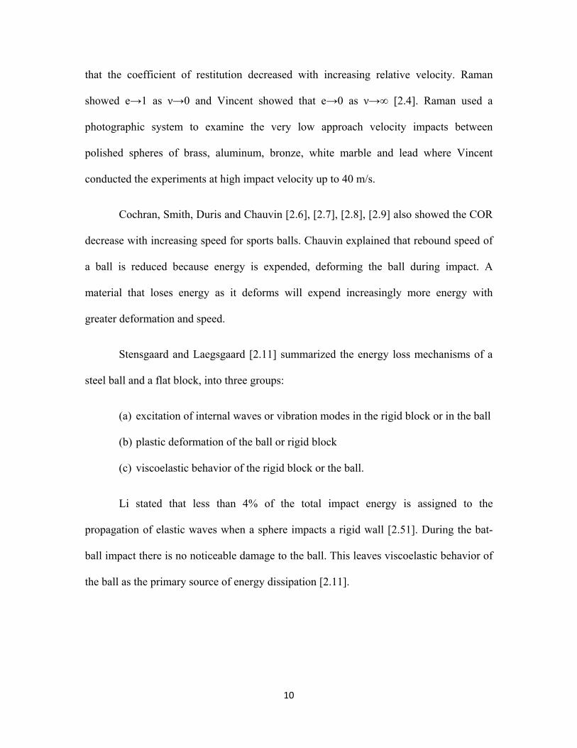
Cochran, Smith, Duris and Chauvin [2.6], [2.7], [2.8], [2.9] also showed the COR

decrease with increasing speed for sports balls. Chauvin explained that rebound speed of

a ball is reduced because energy is expended, deforming the ball during impact. A

material that loses energy as it deforms will expend increasingly more energy with

greater deformation and speed.

Stensgaard and Laegsgaard [2.11] summarized the energy loss mechanisms of a

steel ball and a flat block, into three groups:

(a) excitation of internal waves or vibration modes in the rigid block or in the ball

(b) plastic deformation of the ball or rigid block

(c) viscoelastic behavior of the rigid block or the ball.

Li stated that less than 4% of the total impact energy is assigned to the

propagation of elastic waves when a sphere impacts a rigid wall [2.51]. During the bat-

ball impact there is no noticeable damage to the ball. This leaves viscoelastic behavior of

the ball as the primary source of energy dissipation [2.11].

11  

2.1.1.b COR Models

Suppose that two balls with masses m1 and m2 collide with velocities ν1 and ν2

respectively. After, collision let m1 recoil with velocity v1 and m2 with velocity v2.

Consider a frame of reference where the center of mass is at rest and the total momentum

remains zero. The total initial kinetic energy Ei and final kinetic energy Ef are [2.3]

⎟⎟⎠

⎞⎜⎜⎝

⎛+=

2

12 121

mmvmE iii and ⎟⎟

⎠

⎞⎜⎜⎝

⎛+=

2

12211 1

21

mmevmE f (2.3)

The fractional energy loss f , which is the ratio of the kinetic energy to the initial kinetic

energy is

f = 1-e2 (2.4)

Hodgkinson [2.12] modeled contact between bodies where linear springs

represent the local compliance of deformation of the small region of contact of each

body. Hodgkinson showed that contact forces can be related to the compression xi in each

spring, as

ii

i xkF

= (2.5)

where Fi is positive in compression and ki is the spring stiffness. The total compression in

the system can be written as:

Fkxtot1

*−= (2.6)

where ( )12

11

1*

−−− += kkk (2.7)

12  

is the sum of the different stiffness and ik are the stiffness of each material, and a value

proportional to Young’s modulus ii Ek ~ or yield strength ii Yk ~ is suggested. When

materials with different stiffness collide, they contribute to the overall COR in proportion

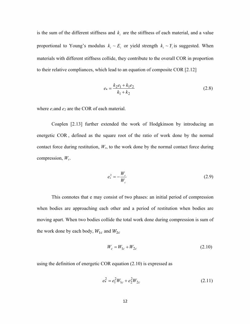
to their relative compliances, which lead to an equation of composite COR [2.12]

21

2112* kk

ekeke++

= (2.8)

where e1and e2 are the COR of each material.

Coaplen [2.13] further extended the work of Hodgkinson by introducing an

energetic COR , defined as the square root of the ratio of work done by the normal

contact force during restitution, Wr, to the work done by the normal contact force during

compression, Wc.

c

r

WWe −=2

* (2.9)

This connotes that e may consist of two phases: an initial period of compression

when bodies are approaching each other and a period of restitution when bodies are

moving apart. When two bodies collide the total work done during compression is sum of

the work done by each body, and

ccc WWW 21 += (2.10)

using the definition of energetic COR equation (2.10) is expressed as

cc WeWee 2221

21

2* += (2.11)

13  

where is the composite COR and is the COR for each body. The energy stored at

the end of the compression phase of each body can be found by assuming linear

constitutive behavior, and is the product of spring stiffness and square of compression on

each spring. The total energy stored in the system at the end of the compression phase is

2

222

211 xkxkWc+

= (2.12)

Following Newton’s third law Coaplin arrived at

21

212

2212

* kkekeke

++

= (2.13)

Equation 2.8 and 2.13 describe a system COR as a function of the individual COR and

stiffness of the impacting bodies. Equation 2.13 is generally preferred since it was

developed from energy considerations, while equation 2.8 is an empirical relation. The

rate dependence of the ball complicate measuring its stiffness. In the following we will

present a method to measure ball stiffness under deformation rates representative of play.

This will improve the estimate of system COR through equations like 2.13.

2.1.2 Dynamic Ball Hardness

Most of the work on ball hardness has been towards human safety. Ball hardness

can be quantified through a so called dynamic stiffness, which can be viewed from the

perspective of the impact force. This can be found by firing a ball at a rigid wall and

measuring the impact force [2.14]. The unknown ball displacement can be replaced by

the measured force, assuming the ball acts as a non-linear spring during the loading phase

[2.15] according to

14  

nkxF = (2.14)

where k and n are the unknown spring constants and F and x are the force and

displacement of the spring respectively. Equating the initial kinetic energy of the ball to

the potential energy at maximum deformation during impact and solving for k we obtain:

ni

np

n

b vF

nmk 2

1

)1(2 +

⎥⎦

⎤⎢⎣

⎡+

= (2.15)

where is the ball mass, is the peak impact force, and is the incoming ball speed.

Smith [2.16] assumed the ball to act as a linear spring during deformation (n=1), so the

stiffness reduces to:

2

1⎟⎟⎠

⎞⎜⎜⎝

⎛=

pvF

mk (2.16)

Hendee [2.17] demonstrated that higher impact velocities yield higher peak

forces. Impact force increased by an average of 448% when the impact velocity was

increased by 200%. Smith [2.9] found a decrease of 6.5% in the dynamic stiffness if the

ball is fired against rigid cylindrical surface rather than flat surface. Carre [2.18] showed

that in the case of cricket balls as the impact velocity increased, the peak force and

deflection was also increased. The stiffness (found by drop testing and static

compression) was relatively constant.

Giacobbe and Scarton [2.19] introduced another method to measure the dynamic

hardness. A variety of sports balls were dropped from a known height on to three

piezoelectric force transducers attached to impact plate. The frequency (Hz) where the

15  

power spectrum level dropped to -60 dB corresponded to a force amplitude drop of one

half and was called the Scarton Dynamic Hardness (SDH) [2.19]. The slope of the power

spectrum at the SDH point was called the DSDH, where D stands for derivative. The

DSDH is always negative and is defined as

SDH

DSDH γ−= (2.17)

Rearranging

))(( DSDHSDH−=γ (2.18)

where he found that γ is a function of the damping coefficient ξ ;

2

)ln(1

1

⎟⎟⎠

⎞⎜⎜⎝

⎛+

=

CORπ

ξ (2.19)

which can be solved for a known value of COR as

21 ξ

πξ

−

−

= eCOR (2.20)

Scarton’s [2.19] method was used to measure the dynamic hardness for a wide variety of

balls including tennis, golf, softballs, baseballs and hockey pucks.

2.1.3 Construction of Cricket Ball

Every sport ball is made of different materials with different construction. In

some cases the difference in the construction of the samples of the same brand can be

seen clearly, which affects their mechanical properties. There is very little information

16  

available regarding the effect of construction of the cricket ball on its properties. Nicholls

[2.20] used a uniaxial compression test for baseballs to show that when a ball positioned

in a “cover” orientation the force-displacement curve and peak force is greater than on a

“seam” orientation.

Carre and Haake [2.18] used impact testing where a cricket ball was dropped on

load cells from different heights at a speed of 13 mph and quasi-static testing. They found

that the ball deforms more with impacts landing on the seam than impacts landing

perpendicular to seam. This information is important as it can help reduce the severity of

impact injuries on the players. It is important to note the impact speed used is much lower

than the actual playing conditions.

Another study done by Hendee, Greenwald and Crisco [2.17] showed that the

peak force of impact at 60 mph for a traditional baseball is 2.4 times higher than the peak

force of a modified (softer) baseball. The COR of the modified (softer) ball also

decreased more rapidly with increasing impact velocity than the traditional ball.

Fuss [2.22] used a quasi-static compression test on different kinds of cricket balls.

Each ball was loaded up to 9 kN with crosshead speeds of 500, 160, 50, 16, and 5

mm/min. He found that balls with uniform construction have higher stiffness than other

balls. The results show that balls with rubber cores are less stiff than balls with a cork

core at its center.

2.1.4 Ball Model

Several people have used different methods for ball modeling. Sandmeyer [2.26]

used a trial and error method from a known ball COR and contact time with finite

17  

elements. Rate effects were neglected. Mustone and Sherwood [2.23] used a Mooney-

Rivlin material model in LS-DYNA, which accepts the load-displacement curve from

static testing performed at different speeds. Bathke [2.24] used ABAQUS to determine

the properties of the ball numerically. A quasi-static compression test was used to

determine the elastic properties of the components of each layer of the baseball. Although

the layers were elastic, the COR decreased linearly with increasing speed. The speed

effect may be due to a loss in energy to internal vibrations within the baseball. The

coefficient of restitution was too high in his model.

Smith, Shenoy and Axtell [2.25] selected a viscoelastic model for a baseball using

LS-DYNA. The time dependent shear modulus was defined as

teGGGtG β−∞∞ −+= )()( 0 (2.21)

and a constant bulk modulus, k where is the instantaneous shear modulus and ∞is the

long term shear modulus. Quasi-static testing was used to find the long term shear

modulus whereas constants and β were found by fitting the experimental load-time

curve. The ∞ was found by

)1(2 ν+

=∞

EG (2.22)

where E and ν were found by static tests. The experimental and finite element results for

COR and dynamic stiffness correlated well [2.14].

Duris [2.9] used Dynamic Mechanical Analysis (DMA) to model the COR and

dynamic stiffness of softballs. Rectangular coupons were machined from the ball core

18  

using a circular saw and milling machine. He used a Prony-series viscoelastic material

model within LS-DYNA defines as

tN

ii

iegtG β−

=∑=

1)( (2.23)

where gi and βi are the shear moduli and the decay constant, respectively. The results did

not agree well with experimental results. The COR and dynamic compression were

observed to be 100% and 50% higher respectively than experimental results.

2.2 Bat Response

2.2.1 Bat Performance metrics

The appraisal of cricket bat performance depends upon many factors. Grant [2.30]

gave five parameters that are needed to determine the bat performance:

The point of impact on the bat

The pre-impact speed of the ball

The pre-impact speed of the bat

The post-impact speed of the ball

The post-impact speed of the bat

The bat with the higher coefficient of restitution will produce a ball with the greatest

post-impact speed. The focus of manufactures has been to improve the COR of the bat.

Fisher [2.31] found that the position of the maximum COR for a cricket bat lies

between 0.19 and 0.23m from the free end of the bat. The bat was impacted at every

0.06m for 9 impact locations where each impact location experienced 6 direct impacts.

19  

The position closest to the free end had very low COR. The initial speed used for this

study was 9m/s (20mph) which was lower than actual playing conditions.

Bryant [2.35] claimed that there is an effective area where performance of the bat

is maximum. The tests involved six collegiate baseball players, the pitch speed was

relatively constant in a range of 54-59mph. 180 hits on each bat were measured, and the

mean hit-ball speeds were 88.6mph for wood bats and 92.4mph for aluminum bats.

2.2.2 Field Conditions

Bowlers use three kinds of bowling deliveries [2.10]: fast bowling, medium pace

or swing bowling and spin bowling. Fast bowlers deliver the ball at speeds in excess of

80mph where the mean ball speed at release is 86mph. Medium paced or swing bowlers

deliver the ball between 65mph and 80mph with a mean ball release speed of 73mph.

Spin bowlers deliver the ball at 40mph and 60mph with a mean ball release speed of

51mph. Justham [2.10] noted that the fastest average speed occurs in test match and

slowest average speed occurs at 20: 20 match.

The motion of the cricket bat is similar to that baseball or softball bat. Adair

[2.32] showed that the swing of the baseball bat is very complex and consists of a

combination of translation and rotation. For a particular input energy these two values

describe the swing speed of player. Fleisig [2.33] conducted tests including 16 baseball

collegiate batters with bat weight varying from 28-32 ounces. Bat motion was analyzed

for 2 frames before impact where the average swing speed was 52-65mph or 1940-2720

degrees per second. Bahill and Freitas [2.34] also reported a swing speed as 55-63 mph

for a college softball batter swinging the bat at imaginary ball.

20  

Nicholls [2.36] studied the effect of bat moment of inertia on ball exit velocity.

The study included 17 (10 right handed and 7 left hander) participants from the

Australian baseball league. Each player hit with both wood and metal bats. High-speed

video was collected using an electronically synchronized 200-Hz camera. Results

revealed that the bat exit velocity was 6.5% lower for wooden bats which had 22% higher

MOI than the metal bats.

More impulse is required to change the bat speed or direction as the MOI is

increased. Therefore, greater MOI compromises the batsman’s ability to control the path

and bat velocity as it swings towards the ball. A field study conducted by Smith [2.38]

on mass and moment of inertia involved 16 amateur slow-pitch softball players of two

skill levels. The study included two groups of bats where one group had constant weight

and other group had constant MOI. The average pitch speed was 23mph. The bat mass

and MOI in this study ranged from 24.5 – 31 oz and 7000 – 11000 oz-inch2, respectively.

Bat swing speed had an observable dependence on the bat MOI, while it was independent

of the bat weight.

A recent study conducted by Cross [2.40] supports Smith’s research on the effect

of bat mass and MOI on swing speed. Six different rods were used, where three rods had

the same swing mass but their MOI differed by a factor of 11. The other three rods had

the same MOI but differed in swing mass by a factor of 2.7. The length was varied to

achieve the large variation. It was found that swing speed decreased with increasing

MOI. It was shown that the bat mass had only a small effect on the swing speed.

21  

Another study on swing speed was conducted by Koenig [2.39] swinging a bat at

both a pitched and stationary ball. Bat speeds varied from 43.5 – 79.5mph. A 10%

increase in MOI produced a 4mph decrease in bat swing speed.

2.2.3 Bat Composition

Advanced materials help improve bat performance without violating the rules of

the game. Such advancements, together with use of stiff and lightweight composite

materials, have engendered many designs. Innovation is limited in cricket where the rules

insist that the blade be made of wood [2.41].

Bryant [2.42] showed that the performance of wooden bat is lower than aluminum

bats. A similar study was done by Greenwald [2.43] on two aluminum bats and wooden

bats. The hit-ball speed of the wood bats exceeded 101mph whereas the aluminum bat

exceeded 106mph. Similar results were found by Shenoy [2.25].

A recent study was done by Stretch [2.44] to compare the rebound characteristics

of wooden and composite cricket bats. In this study two composite, three English willow

and one Kashmir willow bats having similar weight and shape were compared at impact

speeds of 42, 63 and 81 mph. It was found that the average rebound speed of the

composite bats was lower than the traditional willow bats at all the three incoming

speeds. The rebound speed of the Kashmir willow was almost 20% lower than the

traditional English willow at all the three approaching speeds.

Most of the modern cricket bat designs are ineffective at increasing the frequencies of

flexural vibration. The factors that might make significant improvement in bat

performance are[2.41]:

22  

1. Increasing the diameter of the handle

2. Removing the damping material (rubber strips) from the handle

3. Increasing the thickness of the bat

A recent study was conducted by Hariharan [2.37] on bat performance with various

impact combinations. Model analysis was used to determine the region where the

maximum ball exit velocity was located. It was found that the region for maximum ball

exit velocity in the finite element model was between 0.72m and 0.8m from the top of the

bat.

2.2.4 Bat Numerical Model

A study was conducted by Zandt [2.45] to determine the hit-ball speed or batted-

ball speed and bat behavior. A numerical method was developed to represent the bat as a

series of slices. A comparison of a rigid, and elastic bat with only the first mode of

vibration was conducted. It was concluded that the first mode of bat vibration was the

dominant mode. This method was further used by Cross [2.46] in which an aluminum

beam was used, which also showed that the first mode of vibration was the dominant

mode.

Shenoy [2.25] used LS-DYNA to model the dynamic interaction of a bat and ball.

The model consisted of 8-noded solid elements for the ball and wooden bat. Four-noded

Hughes Liu shell elements were used for the aluminum bat. The numerically obtained hit-

ball speeds correlated well with those obtained experimentally. Penrose [2.47] used two

different methods involving finite element bat/ball models. In the first model isotropic

properties are used for bat. The ANSYS/LS-DYNA package was used for second model

23  

of a bat/ball impact where two basic designs were modeled for comparison. Orthotropic

properties were used as the bat material. The two methods showed good correlation with

each other.

John [2.48] studied the deflection of cricket bats experimentally and numerically.

His experimental work involved modal analysis with a clamped handle. His numeric

model constrained the proximal end of the bat. The bat vibrational frequency was

measured from ball impacts in the numerical model and compared with experiment. The

FEM model showed good agreement with experimental results, suggesting that the FEM

model is a feasible numerical tool to predict the performance of a cricket bat. It was

observed that the performance of the bat varied with impact location.

Grant [2.41] used a finite element model to compare the performance of a variety of

designs. The basic model was correlated to experimental data. Agreement improved

when the density of the wood was increased by 50% from that found in the literature. It

was observed that the mode one and two frequencies were identical whereas third mode

was 4% lower.

2.2.5 Bat Constraint

Constraint is an important factor to determine bat performance. Brody [2.49]

used two softballs, one wood and one-aluminum bat to experimentally measure vibration.

Comparison of the vibrational response between freely, hand held and vice clamped bats

was done. The freely suspended bat had the same vibrational response as the hand-held

bat but there was a difference in the vibrational response in the clamped bat. He

24  

concluded nevertheless that grip firmness should not determine the post-impact velocity

of the ball.

Fisher [2.50] measured the hand loads on five different commercial bats. Three

clamping configurations were employed on rigid clamps, in a hand simulator, and hands

of a human subject. The clamps were positioned 210mm apart and rigid clamps were

tightened to 300N, whereas hand the simulator was tightened to 8 N, equal to human grip

force. The impact positions were at 6cm intervals from the end of the bat, impacted from

a ball drop tube at 9m/s. He found that the hand simulator clamped loads were very

similar in distribution to hand loads, for the load measured along the length of the bat. It

was also observed that the rigid clamped grip load was ten times the magnitude of the

hand-held bat.

Weyrich [2.51] used aluminum and wooden bats to study the effect of grip

firmness and bat composition. Bats were clamped in a vise or freely suspended. Three

impact locations were used: center of percussion, center of gravity and the end of the bat.

The rebound velocities for impacts at the center of gravity for the wooden bat were the

same for clamped and freely suspended constraints. It further signifies that the constraints

do not affect the performance of the bat.

2.3 Summary

The purpose of this chapter was to review the historical and current research

relevant to bat performance. In doing so, ball and bat testing methods have been

discussed. Experimental and finite modeling methods have been explained. The most

significant contribution revolves around finite element modeling of cricket balls and bats.

25  

In the following chapters, experimental bat and ball testing along with numeric

modeling will be presented. The dynamic properties of the ball has a great effect on the

performance of the bat. The variation in construction which effects the dynamic response

of the cricket balls will be discussed in the following chapter. Comparison between

different types of wood species and composite materials will be conducted. An extensive

study regarding the ball and bat finite element models will be carried out and verified

with experimental results. The effect of weight distribution on the bat finite element

model will also be studied.

26  

REFERENCE

[2.1] Barnes, G. “Study of collisions”. Am. J. Phys. 26, p. 5-12. 1957.

[2.2] ASTM F 1887-02. “Standard test method for measuring the coefficient of restitution of baseballs and softballs.” West Conshohocken, Pa. 2003.

[2.3] Cross, R. “The coefficient of restitution for collisions of happy balls, unhappy balls, and tennis balls”. Am. J. Phys. 68 (11), p. 1025-1031. 2000.

[2.4] Barnes, G. “Study of collisions”. Am. J. Phys. 26, p. 5-12. 1957.

[2.5] Brody, H. “The physics of tennis. III. The ball-racket interaction”. Am. J. Phys. 65 (10), p. 981-987. 1997.

[2.6] Chauvin, D.J., Carlson, L.E. “A comparative test method for dynamic response of baseballs and softballs. International Symposium on Safety in Baseball/Softball”. ASTM STP 1313, p. 38-46. 1997.

[2.7] Cochran, A.J. “Development and use of one dimensional models of a golf ball”. J. Sports Sciences. Taylor and Francis, Ltd. London, UK. 2002.

[2.8] Strangwood, M., Johnson, A.D.G., Otto, S.R., “Energy losses in viscoelastic golf balls”. Proc. IMechE, Vol.220 Part L, Journal of Materials: Design and Applications, pp. 23-30. 2006.

[2.9] Duris, J.G and Smith, L.V. “Evaluation test methods used to characterize softballs”. The Engineering of Sport 5, Vol 2, pp. 80-86. ISBN: 0-9547861-1-4. Davis, CA. 2004.

[2.10] Justham, L.M., West, A.A., Cork, A.E.J., “An Analysis of the differences in bowling technique for Elite Players during International Matches” The impact of technology on Sports,pp.331-336. 2007

[2.11] Stensgaard, I., Laegsgaard, E. “Listening to the coefficient of restitution-revisited”. Am. J. Phys. 69 (3), p. 301-305. 2001.

[2.12] Hodgkinson, E. “On the collision of imperfectly elastic bodies”. Report of the fourth Meeting of the British Association for the Advancement of Science. 1835.

[2.13] Coaplen, J., Stronge, W.J., Ravani, B. “Work equivalent composite coefficient of restitution”. Int. J. of Impact Engrg. 30, p. 581-591. 2004.

[2.14] Duris, J.G. “Experimental and Numerical characterization of softballs”. Master thesis. Washington State University. 2004.

27  

[2.15] Smith, L.V., Duris, J.G., Nathan, A.M. “Describing the dynamic response of Softballs” Unpublished.

[2.16] Smith, L.V., Biesen, E. “Describing the plastic deformation of aluminum softball bats”. The impact of technology on Sports, pp.351-356. 2007

[2.17] Hendee, S.P., Greenwald, R.M., Crisco, J.J. “Static and Dynamic properties of various baseballs”. J. App. Biomech. 14, p. 390-400. 1998.

[2.18] Carre, M.J., James, D.M., Haake, S.J. “Impact of a non-homogeneous sphere on a rigid surface”. Proceeding of the institution of Mechanical Engineers, Journal of Mechanical Engineering science. Vol. 218 Part C: pp. 273. 2004

[2.19] Giacobbe, P.A., Scarton, H.A., Lee, Y.S. Dynamic hardness (SDH) of baseballs and softballs. International Symposium on Safety in Baseball/Softball. ASTM STP 1313, p. 47-66. 1997.

[2.20] Nicholls, R.L., Miller, K., Elliott, B.C., “Modeling deformation behavior of the baseball”. Journal of applied biomechanics. pp. 18-30. 2005.

[2.21] Bartel, D.M., Yagley, M.S., Dewanjee, P.K. “Golf ball with high Coefficient of Restitution” United States Patent. Patent No: US 6,648,775 B2, 2003.

[2.22] Justham, L.M., West, A.A., Cork, A.E.J., “Non-Linear viscoelastic properties and construction of cricket balls” The impact of technology on Sports, pp.331-336. 2007

[2.23] Mustone, T.J., Sherwood, J.A. “Using LS-Dyna to characterize the performance of baseball bats”. Unknown source.

[2.24] Bathke, T. “Baseball impact simulation”. Senior mech. eng. thesis, Brown University. 1998.

[2.25] Smith, L.V., Shenoy, M.M., Axtell, J.T., “Performance assessment of wood, metal and composite baseball bats”. ASME IMECE, 2000.

[2.26] Sandmeyer, B.J. “Simulation of bat/ball impacts using finite element analysis”. Master’s thesis, Oregon State University. 1994.

[2.27] Bowen, R., “Cricket: A History of its growth and development throughout the world”. Eyre and Spottiswoode. London. 1970 [2.28] The laws of Cricket – 2000 Code, Marylebone Cricket Club, London, 2000

[2.29] John, S., Li, Z.B. “Multi-directional vibration analysis of cricket bats” The engineering of Sports, 2002

28  

[2.30] Grant, C., Davidson, R.A. “Design of a Cricket bat test machine” Proceeding of the second international conference on the engineering of sports, Blackwell Science, Oxford, pp41-48, 1998

[2.31] Fisher, S., Vogwell, J. “The dead spot of the tennis racket” Am. J. Phys. Vol 65, pp 754-764. 1997

[2.32] Adair, R. K. “The Physics of baseball” 2nd Edition, 1994

[2.33] Fleisig, G. S., Nigel, Z., David, S., Andrew, J. R., “The relationship among baseball bat weight, moment of inertia, and velocity” Am. Sports Medicine Ins., August 20, 1997

[2.34] Bahill, A.T., Freitas, M. M. “Two Methods for recommending bat weight” Annals of Biomedical Engineering, pp: 436-444, 1995

[2.35] Bryant, F. O., Burkett, L. N., Chen, S. S., Krahenbuhl, G. S., Lu, P. “Dynamic and performance characteristics of baseball bats” Research Quarterly Exercise Sports, 1979

[2.36] Nicholls, R. L., Elliott, B. C., Miller, K., Koh, M. “Bat kinematics in baseball: Implication for ball exit velocity and player safety” Journal of Applied Biomechanics 19, pp: 283-294, 2003

[2.37] Hariharan, V., Srinivasan, P. S. S. “Inertial and vibration characteristics of a cricket bat” vibrationdata.com

[2.38] Smith, L., Broker J., Nathan A., "A Study of Softball Player Swing Speed," in: Sports Dynamics Discovery and Application, Edited by Subic A., Trivailo P., and Alam F., (RMIT University, Melbourne Australia), pp: 12-17, 2003

[2.39] Koenig, K., Hannigan, T., Davis, N., Hillhouse, L. “Inertial effect on Baseball Bat Swing Speed” 1997

[2.40] Cross, R., Bower, R. “Effects of Swing-Weight on swing speed and racket power” journal of Sports Sciences, pp: 23-30 January 2006

[2.41] Grant, C. “The role of the materials in the design of an improved cricket bat” MRS Bulletin. March 1998

[2.42] Bryant, F. O., Burkett, L. N., Chen, S. S., Krahenbuhl, G. S., Lu, P. “Dynamic and performance characteristics of baseball bats” Rec. Q. Exerc. Sport, pp: 505-510, 1979

[2.43] Greenwald, R. M, Penna, L. H., Crisco, J. J., “Difference in batted ball speed with wood and Aluminum baseball bats: A batting cage study” J. Appl. Biomech., 17, pp: 241-252, 2001

[2.44] Stretch, R. A., Brink, A., Hugo, J. “A comparison of the ball rebound characteristics of wooden and composite cricket bats at three approach speeds” Sports Biomechanics, Vol 4, pp: 37-46, 2006

29  

[2.45] Zandt, V. L. L. “The dynamical theory of the baseball bat” American Journal of Physics, February, 1992

[2.46] Cross, R. “Impact of a ball with a bat or racket” American journal of Physics, August, 1999

[2.47] Penrose, J. M. T., Hose, D. R. “Finite element impact analysis of a flexible cricket bat for design optimization” The engineering of sports. 1998

[2.48] John, S., Li, Z.B. “Multi-directional vibration analysis of cricket bats” Proceedings of the 4th International Conference on the Engineering of Sport. Held in Kyoto, Japan, September 3rd-6th, Published in ‘The Engineering of Sport 4’, Editors Ujihashi S & Haake S J, pp 96-103, 2002. ISBN 0632 06481 1, 2002

[2.49] Brody, H. “Model of baseball bats” American journal of Physics, August 1990

[2.50] Fisher, S., Vogwell, J., Ansell, M. P. “Measurement of hand loads and the centre of percussion of cricket bats” Journal of Materials: Design and applications, Proc. IMechE Vol.220, 2006

[2.51] Li, L-y., Thornton, C., Wu, C-y. Impact behavior of elastoplastic spheres with a rigid wall. Proc. Instn. Mech. Engrs. 214 (C). 2000.

30  

CHAPTER 3

-BALL TESTING-

3.1 Introduction

Cricket balls are made from cork at the nucleus surrounded by several layers of

tightly wound string, and covered by a leather case with a slightly raised seam. The

covering of the leather case is constructed of four pieces, but the hemispheres are rotated

by 90 degrees with respect with each other. The equator of the ball is stitched to form six

rows, whereas the remaining two leather seams are hidden stitched. The cricket ball

measures between 8 13/16 and 9 inches (22.4 and 22.9 cm) in circumference and weighs

between 5.5 and 5.75 ounces (155.9 and 163.0 g). There are a number of ways to

construct cricket balls, with varying core designs [3.1]. Cricket balls are machine or

handmade. Conventionally, cricket balls of red color are used in test matches and first-

class cricket; whereas white balls are used in one day international cricket matches as

shown in Fig. 3.1.

Figure 3.1: Cricket balls used in test, first-class and one-day international cricket

matches.

31  

There is little data regarding the impact properties of cricket balls but the impact

speed has been measured. Studies showed that the release speed from the bowlers hand is

100mph and the speed at the batting end after rebounding from the pitch is 80mph. The

maximum ball velocity at the batter end was recorded in the 1999 world cup Tournament

was 93mph [3.2].

3.2 Ball Testing Apparatus

An experimental apparatus has been designed that minimizes the variability in

pitch speed, impact location, and spin of the ball. An apparatus was designed in which

both the COR and dynamic stiffness of the ball can be measured. A schematic of the test

apparatus is shown in Fig. 3.2.

Figure 3.2: Cricket ball test schematic.

The experimental apparatus consisted of the canon, light curtains, load cells, rigid

wall and a desktop computer. The canon setup consisted of a large accumulator where the

pressure within the air tank was controlled by a regulating valve connected to the

computer. The desired pitch speed was achieved by adjusting the pressure in the

32  

accumulator tank. The ball was placed at the breach end of the barrel which closed by

pneumatic cylinders. Fig. 3.3 shows the cannon’s air accumulator tank, breach plate, and

barrel.

A sabot was used to load the ball in the barrel to ensure proper centering and that

the ball was not spinning after being fired. The sabot was made of polycarbonate, as

shown in Fig. 3.4. On the other side of the barrel an arrestor plate prevented the sabot

from traveling in the light curtain, where the ball velocity before and after the impact was

measured. Three pairs of ADC light gates (Automated Design) were used to measure the

incident and rebound speeds of the cricket balls. The arrestor plate, light gates, rigid

plate, and load cells are showed in Fig. 3.5.

Figure 3.3: Cannon accumulator tank, breach plate, and barrel.

33  

Figure 3.4: The sabot, Cricket ball and the supporter.

Figure 3.5: Cannon arrestor plate, light gates, rigid plate, and load cells.

34  

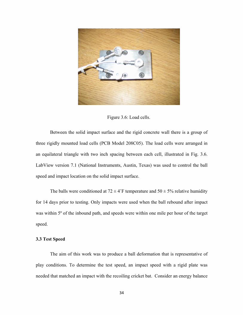
Figure 3.6: Load cells.

Between the solid impact surface and the rigid concrete wall there is a group of

three rigidly mounted load cells (PCB Model 208C05). The load cells were arranged in

an equilateral triangle with two inch spacing between each cell, illustrated in Fig. 3.6.

LabView version 7.1 (National Instruments, Austin, Texas) was used to control the ball

speed and impact location on the solid impact surface.

The balls were conditioned at 72 ± 4˚F temperature and 50 ± 5% relative humidity

for 14 days prior to testing. Only impacts were used when the ball rebound after impact

was within 5º of the inbound path, and speeds were within one mile per hour of the target

speed.

3.3 Test Speed

The aim of this work was to produce a ball deformation that is representative of

play conditions. To determine the test speed, an impact speed with a rigid plate was

needed that matched an impact with the recoiling cricket bat. Consider an energy balance

35  

for an impact between a freely moving cricket bat (rotating mass) and a moving cricket

ball (point mass).

The relationship between the cricket ball speed and the swing speed of cricket bat

can be found by considering the impact speed between a cricket ball and rigid blocks

with different masses m1 and m2. The cricket ball impacts the stationary blocks 1 and 2

with an initial velocity of V1 and V2, respectively. Let mb be the mass of cricket ball with

stiffness k. Both the cricket ball and block move with same speed, v at the point of

maximum displacement, xp, The energy balance is then

222 )(21

21

21

iibiip vmmkxVm ++= (3.1)

where i= 1 or 2 for collision between the cricket ball and block 1 and 2, respectively.

Momentum is conserved during the impact according to

iibib vmmVm )( += (3.2)

Equation (3.1) and (3.2) may be combined to eliminate vi as

)(

2222

ib

ibpib mm

VmkxVm+

+= (3.3)

If the impacts with block1 and 2 are identical the ball displacement should be the same

for each case. By evaluating Eq. 3.3 for block 1 and 2, xp may be eliminated to produce

36  

2/1

2

121

1

1

⎟⎟⎟⎟⎟

⎠

⎞

⎜⎜⎜⎜⎜

⎝

⎛

+

+=

mmmm

VVp

p

(3.4)

For the case when the block 1 is infinitely large, m1 becomes infinity, so mp/m1

approaches zero.

For the scenario of swinging object, m2 becomes the swing-weight or I/b2 where I

is the moment of inertia and b is the distance between the impact location and the pivot

point. Substituting Eq. (3.1) into Eq. (3.4) results in

2/1112 )1( rvv += (3.5)

where v2 and v1 are the incoming ball speeds in the rigid wall tests and play, respectively.

The bat recoil factor, ri is defined as

i

bi I

bmr2

= (3.6)

where mb is the mass of the cricket ball, b is the distance between the impact location and

the pivot point of the cricket bat, and I is the mass moment of inertia of the bat with

respect to the pivot point [3.7]. Using a cricket bat pivot distance of 22 inches with 9800

oz.in2 mass moment of inertia, a bat-ball relative speed of 60mph and cricket ball of 5.65

oz, the rigid wall ball speed is 53 mph.

37  

3.4 Dynamic Properties

The performance of the cricket ball can be compared by its coefficient of

restitution (e), (ASTM 1887 [3.5]). The ball was impacted on four sides: two faces and

two seams. The ball was rotated o90 after every impact so that each face and seam of the

ball was impacted one in four times. The coefficient of restitution (e) was measured as

the ratio of the rebound and inbound speeds, as

1

2

Vve −

= (3.7)

where V1 and v2 are the inbound and rebound speeds of the cricket ball, respectively. For

a typical bat, a 2.0% increase in the COR can raise bat performance 1% [3.6].

The hysteresis from loading and unloading of the cricket ball can be described

from the force vs. displacement curve. Displacement was obtained by dividing the force

by the ball mass and integrating it twice, since

bm

Fdt

xd=2

2

(3.8)

where F is the force (lb), mb is the mass of the ball and with the initial conditions x = 0 at

time t = 0 and dx/dt = Vi at time t = 0. Fig. 3.7 shows a sample hysteresis plot for a

cricket ball impacting a flat plate at 70mph.

38  

Figure 3.7: Hysteresis plot of cricket ball impacting at 70mph.

3.5 COR and Dynamics Stiffness Results

In the current study, balls from two different manufactures were used (Ba and Bb)

Fig. 3.8. These balls are regularly used in the First-class cricket in different countries.

The coefficient of restitution, (COR) and dynamic stiffness of six balls of each Ba and Bb

were tested at 53mph. The cricket balls were impacted six times, from which the average

COR and dynamic stiffness was obtained. Fig. 3.9 shows the difference in average COR

and average dynamic stiffness for Ba and Bb. On average, the dynamic stiffness of ball

models Ba was 19% higher than Bb. The average COR values were closer than the

dynamic stiffness, where model Ba was 5% higher than Bb.

The difference in dynamic properties may be due to the difference in the

construction of the cricket balls. Ball model Bb has a uniform construction with a

modeled rubber core where model Ba has a cork core which was only approximately

spherical. The different ball construction and materials likely contribute to their

0

500

1000

1500

2000

2500

3000

3500

4000

4500

0.5 0.55 0.6 0.65 0.7 0.75 0.8 0.85

Force (lb

)

Displacement (in)

39  

characteristic response. In the following, the error bars represent the standard deviation

for each case. The standard deviation of dynamic stiffness was nearly twice that for COR.

Figure 3.8: Cross sectional view of cricket ball Ba and Bb.

Figure 3.9: The average COR and dynamic stiffness of model Ba and model Bb.

0

500

1000

1500

2000

2500

3000

3500

4000

0.00

0.10

0.20

0.30

0.40

0.50

0.60

Ba Bb

Dynam

ic Stiffne

ss (lb/in)

COR

Average CORAverage DS

40  

Cricket balls have a pronounced seem that may produce a different response than

the face. To consider this difference, seam and face impacts were compared between

balls Ba and Bb as shown in Fig. 3.10. The average dynamic stiffness for Ba and Bb at

the seam was 3% higher than the face. The average COR at the seam was 2% higher than

the face. It is thought that the increased stiffness in the seam impact is due to the

presence of the seam itself rather than the construction of the balls. Previous results for

stiffness and hysteresis loss was found from drop test range around 13mph and quasi-

static tests, which is much lower than the test speed used in this study [2.18]. The results

here indicates different trend which may be the test used previously doesn’t correspond to

the actual play conditions.

Figure 3.10: Comparison between the dynamic properties of Ba and Bb.

0

500

1000

1500

2000

2500

3000

3500

4000

0.00

0.10

0.20

0.30

0.40

0.50

0.60

Ba Bb

Dynam

ic Stiffne

ss (lb/in)

COR

COR Face

COR Seam

DS Face

DS Seam

41  

3.6 Rate Dependence

It is important to understand the behavior of the cricket ball under various impact

speeds. Previous studies have shown that the softball and baseball COR decreases

linearly with increasing impact speed [3.7].

In the current study 20 balls, of Ba and Bb were used. The balls were impacted at

speeds ranging from 60mph to 80mph. Each ball was impacted six times; three times on

the seam and three times on the face at each impact speed. Fig. 3.11 shows the average

COR and DS as a function of speed. The COR decreased linearly with increasing impact

speed. The increasing DS as a function of speed shows that cricket ball behaves as non-

linear spring. The DS had a higher variation than COR as shown previously in Fig. 3.10.

Figure 3.11: Average COR and DS as a function of increasing speed.

The DS in Fig. 3.11 was found for a linear spring. A nonlinear spring may be

considered using Eq. 2.15. To determine the degree of nonlinearity, the exponent n was

11000

11500

12000

12500

13000

13500

14000

14500

15000

0.4

0.42

0.44

0.46

0.48

0.5

0.52

55 60 65 70 75 80 85

Dynam

ic stiffne

ss (lb/in)

COR

Impact Speed (mph)

Average CORAverage DS

42  

varied until the stiffness was constant with the speed. Ball model Ba was used for this

study, where k was constant with n=1.27 (Fig 3.12). This response is similar to softball

(n=1.25) and classical Hertzian contact (n=1.5).

Figure 3.12: Linear and non-linear stiffness of the cricket ball impact at different speeds.

The effect of speed on COR of each ball model are compared in Fig. 3.13. It was

found that the difference in COR between the models increased with speed. The different

speed dependence of the ball models suggests that different ball models have a different

rate-dependence, which further may be related to the construction of each ball model.

8000

10000

12000

14000

16000

18000

20000

55 60 65 70 75 80 85

Dynam

ic Stiffne

ss (lb/in)

Impact speed (mph)

n=1

n=1.27

43  

Figure 3.13: Comparison of COR for Ba and Bb models (6 balls at each point).

The dynamic properties of ball can be considered with force-displacement curves.

The force vs. displacement curve for seam and face impacts is plotted for both models as

a function of increasing impact speed in Fig. 3.14-3.17.

Figure 3.14: Representative force-displacement curves for Ba seam impacts.

0.40

0.42

0.44

0.46

0.48

0.50

0.52

55 60 65 70 75 80 85

COR

Speed (mph)

Ba

Bb

0

1000

2000

3000

4000

5000

6000

7000

8000

0 0.1 0.2 0.3 0.4

Force (lb

)

Displacement (inch)

60mph seam65mph seam70mph seam75mph seam80mph seam90mph seam

44  

Figure 3.15: Representative force-displacement curves for Ba face impacts.

Figure 3.16: Force-displacement curve for Bb face impacts.

0

1000

2000

3000

4000

5000

6000

7000

8000

0 0.1 0.2 0.3 0.4

Force (lb

)

Displacement (inch)

60mph Face65mph face70mph face75mph face80mph face90mph face

0

1000

2000

3000

4000

5000

6000

0 0.1 0.2 0.3 0.4

Force (lb

)

Displacement (inch)

60mph face65mph face70mph face75mph face80mph face90mph face

45  

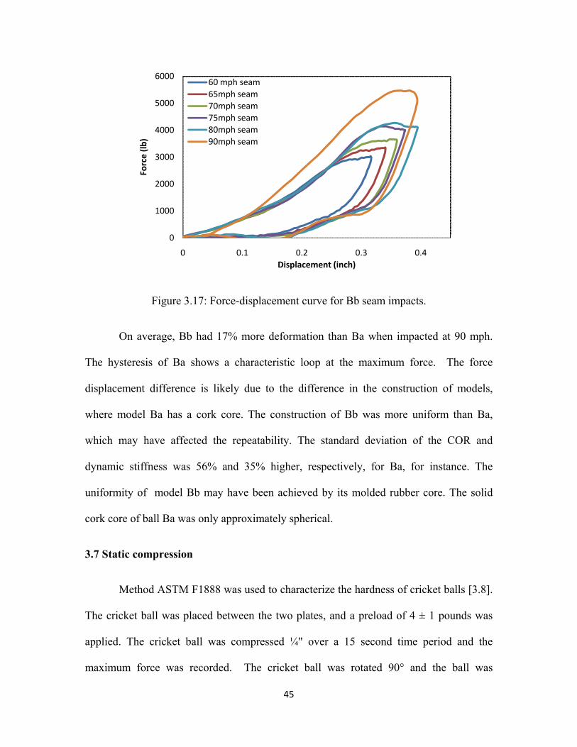
Figure 3.17: Force-displacement curve for Bb seam impacts.

On average, Bb had 17% more deformation than Ba when impacted at 90 mph.

The hysteresis of Ba shows a characteristic loop at the maximum force. The force

displacement difference is likely due to the difference in the construction of models,

where model Ba has a cork core. The construction of Bb was more uniform than Ba,

which may have affected the repeatability. The standard deviation of the COR and

dynamic stiffness was 56% and 35% higher, respectively, for Ba, for instance. The

uniformity of model Bb may have been achieved by its molded rubber core. The solid

cork core of ball Ba was only approximately spherical.

3.7 Static compression

Method ASTM F1888 was used to characterize the hardness of cricket balls [3.8].

The cricket ball was placed between the two plates, and a preload of 4 ± 1 pounds was

applied. The cricket ball was compressed ¼" over a 15 second time period and the

maximum force was recorded. The cricket ball was rotated 90° and the ball was

0

1000

2000

3000

4000

5000

6000

0 0.1 0.2 0.3 0.4

Force (lb

)

Displacement (inch)

60 mph seam65mph seam70mph seam75mph seam80mph seam90mph seam

46  

compressed again. Figure 3.20 and 3.21 shows the fixture for both seam compression and

face compression. The average of two peak forces was taken as the static compression.

The average static compression of 33 balls of Ba and Bb was measured. Fig. 3.18

represents the static compression and dynamic stiffness of the cricket balls. The

compression of model Ba was 135% higher than Bb. The difference decreased for

dynamic stiffness measured at 60mph, where Ba was 37% stiffer than Bb. Fig. 3.19

shows the comparison between the face and seam static compression of ball models Ba

and Bb. It can be seen that, on average face static compression is 16% higher than seam

static compression. The study done previously [2.18] on the face and seam compression

shows opposite results from this study. In this study, both the dynamic stiffness and

static compression shows the same end results. In this study dynamic stiffness, the

impact speed used is representative of the playing conditions, whereas the impact speed

of the previous study was much lower.

Figure 3.18: Static and dynamic stiffness of cricket balls.

0

2000

4000

6000

8000

10000

12000

14000

16000

18000

0

100

200

300

400

500

600

700

800

900

Ba Bb

Dynam

ic stiffne

ss (lb/in)

Static com

pression

 (lbs)

Static Compression

Dynamic Stiffness

47  

Figure 3.19: Face and seam static compression of ball model Ba and Bb.

Figure 3.20: Seam Compression of the cricket ball.

0

100

200

300

400

500

600

700

800

Face Seam

Static Com

pression

 (lbs)

Ba

Bb

48  

Figure 3.21: Face compression of the cricket ball.

3.8 Summary

The goal of this study was to evaluate the COR and dynamic stiffness of various

cricket balls. The results show that the COR of all the balls decrease with increasing

impact speed. The dependence of COR on speed appeared to be related to the ball

construction.

Seam impacts had higher COR and higher dynamic stiffness than a face impacts.

The dynamic stiffness increased with speed using a linear spring model. A gradual

increase in displacement and force with the impact speed was observed. The peak

displacement shows linear relationship with impact speed. The relationship between peak

force as a function of impact speed is non-linear. This may be due to the construction of

the cricket ball models. Results reveal that the ball Ba which contains rubber core have

49  

lower COR than ball Bb with cork core. It suggests that the different ball construction

most likely contribute to their dynamic response.

50  

REFERENCES

[3.1] The laws of Cricket – 2000 Code, Marylebone Cricket Club, London, 2000

[3.2] Tom P., Daryl F. and Brain B. “Release Velocities of fast bowlers during a cricket test match” Supplement to the Australian Journal for Health, Physical Education and Recreation. March 1976 [3.3] Carre, M.J., James, D.M., Haake, S.J. “Impact of a non-homogeneous sphere on a rigid surface”. Proceeding of the institution of Mechanical Engineers, Journal of Mechanical Engineering science. Vol. 218 Part C: pp. 273. 2004 [3.4] Nathan, A. M. “Characterizing the Performance of Baseball Bats” Am. J. Phys, 71 (2). February 2003 [3.5] ASTM F 1887 Standard Test Method for Measuring the Coefficient of Restitution

(COR) of Baseball and Softballs, ASTM International 2004. [3.6] Adair, R.K. The physics of baseball. New York, Harper and Row, 3rd edition. 2002.

[3.7] Chauvin, D.J., Carlson, L.E. A comparative test method for dynamic response of baseballs and softballs. International Symposium on Safety in Baseball/Softball. ASTM STP 1313, p. 38-46. 1997.

[3.8] Nathan, A. M. 2003. Characterizing the Performance of Baseball Bats, American Journal of Physics, 71.2:134-143.

[3.7] Smith, L. V. Measuring the Hardness of Softballs, Abstract Proc. of the Society for Experimental Mechanics, Spring Conference, Orlando, Florida, 2008

[3.8] ASTM F1888-04 Standard Test Method for Compression-Displacement of Baseballs and Softballs, ASTM International, Pennsylvania (2004).

51  

CHAPTER 4

-BAT TESTING-

4.1 Introduction

The aim of the bat is to send the ball to its home by playing the most powerful

shot, and minimizing shock to the batsman’s hand. The blade is commonly made of

English or Kashmir willow which is strong, lightweight and has good shock resistance.

The handle is made of cane which has good shock absorbing properties. As shown in

Fig. 4.1 the length of the bat cannot exceed 38 inches (96.5 cm) and the width of the

blade must be less than 4.25 inches (10.8 cm) [4.2]. A material can be used to protect,

repair or strengthen the blade of the bat; but must be limited to 1/16inches (1.56mm) in

thickness and may not cause any harmful damage to the ball. There is no law covering

the weight of the cricket bat [4.2].

Figure 4.1: Dimensions of Cricket bat according to Law 6 [4.2].

52  

During the manufacture of a bat, the blade is compressed (knocked) in order to

resist the dynamic impact of the ball without getting damaged. Little has been done,

however, to consider the effect of knock-in or wood species on performance. Studies

have shown that the surface hardness of the cricket bat increases with knocking, which

produces a stiff and dense region that affects the flexural stiffness and vibration of the bat

[4.3], [4.4]. Recent advances in technology and materials have motivated a number of

changes in cricket bat design. Advanced composite materials are used to stiffen the blade

and is purported to improve durability. While some studies suggest these advances have

not affected performance, more work is needed to quantify their contribution [4.5].

The current study compares the effect of surface hardness, wood species and

composite reinforcement on the performance of the cricket bats. An experimental test

apparatus was developed to measure the performance of cricket bats under dynamic

impact conditions representative of play. A bat performance measure was derived in

terms of an ideal batted-ball speed based on play conditions.

The performance of five cricket bats with different structural, geometrical and

material properties was measured. Bats manufactured from Kashmir willow, English

willow and with a composite skin were compared. The bats were identified by a code,

where the first character indicated the material (K=Kashmir, E=English willow), the

second letter was the sequential number of the cricket bat, followed by the third letter for

knock-in or unknock-in (Knock-in=K, Unknocked=U). As there was only one composite

bat the code for the cricket bat with and without a composite skin was CS and CWS

respectively. For example E2U means the bat material is English willow, it is 2nd bat in

the order and it is unknocked.

53  

4.2 Experimental Apparatus setup

4.2.1 MOI Apparatus

The swing speed of the bat depends upon the swing-weight, which is described by

the MOI of the bat [4.6]. The MOI of the cricket bat was determined by ASTM F2398-

04 (used to measure the MOI of the baseball and softball bats) [4.7]. The MOI of the

cricket bat was measured as a physical pendulum, rotating about a pivot 6 inches from the

end of the handle [4.8]. The apparatus used to measure the moment of inertia of the

cricket bat is shown in the Fig. 4.2. The bat was placed on the MOI apparatus so that the

bat could swing freely on the clamp pivot points. The average of five repeatable readings

with 10 oscillations for each reading was used to measure the MOI of the cricket bat. The

acceptable average standard deviation of each reading was 0.0005sec.

Figure 4.2: Experimental apparatus used to measure the MOI of the cricket bat.

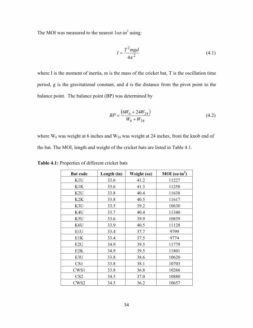
54  

The MOI was measured to the nearest 1oz-in2 using:

2

2

4πmgdTI = (4.1)

where I is the moment of inertia, m is the mass of the cricket bat, T is the oscillation time

period, g is the gravitational constant, and d is the distance from the pivot point to the

balance point. The balance point (BP) was determined by

( )

246

246 246WW

WWBP++

= (4.2)

where W6 was weight at 6 inches and W24 was weight at 24 inches, from the knob end of

the bat. The MOI, length and weight of the cricket bats are listed in Table 4.1.

Table 4.1: Properties of different cricket bats

Bat code Length (in) Weight (oz) MOI (oz-in2) K1U 33.6 41.2 11227 K1K 33.6 41.3 11258 K2U 33.8 40.4 11638 K2K 33.8 40.5 11617 K3U 33.5 39.2 10630 K4U 33.7 40.4 11340 K5U 33.6 39.9 10839 K6U 33.9 40.5 11128 E1U 33.4 37.7 9799 E1K 33.4 37.5 9774 E2U 34.9 39.5 11779 E2K 34.9 39.5 11801 E3U 33.8 38.6 10620 CS1 33.8 38.1 10703

CWS1 33.8 36.8 10266 CS2 34.5 37.0 10880

CWS2 34.5 36.2 10657

55  

4.2.2 Bat Testing Equipment

The bat was tested using the fixture similar to the ball test as shown in Fig. 4.3,

where the rigid wall was replaced by a pivot assembly as shown in Fig. 4.4. The pivot

assembly allowed the bat to recoil after impact and controlled the impact location. Three

pairs of ADC iBeam light gates were used to measure the inbound and rebound speed of

the cricket ball. LabVIEW version 7.1 was used to record and reduce the data and control

the impact location of the cricket bat on the pivot assembly.

In the bat tests an incoming ball speed of 60 mph was used to prevent

accumulated bat damage from influencing the results. Each bat was impacted at ½ inch

increments to find the location with maximum performance. An average value from six

balls impacting the blade of the bat was used to determine the maximum performance.

The ball was rotated along the common axis so that face and seam impacts occurred at

each location.

Figure 4.3: Experimental test fixture used to test cricket bats.

56  

Figure 4.4: Pivot assembly used to test cricket bats.

4.3 Bat Performance Metric

Light gates measured the ball speed before and after impact. The ratio of the

rebound to inbound ball speed is the so-called collision efficiency, ea [4.9]

1

2Vvea

−= (4.3)

where v2 and V1 are the ball speeds after and before impact, respectively. The negative

sign indicates that the cricket ball travels in the reverse direction after impact with bat. If

the bat speed, vb, and ball speed, vp, in play conditions are known, the collision efficiency

may be used to find the batted ball speed, BBS in play, according to

bapa veveBBS )1( ++= (4.4)

57  

The bowled ball speed is relatively easy to measure in play and is usually taken as a

constant when comparing bat performance. In this work it was taken as 85 mph.

The bat speed is more difficult to measure and has a greater effect on the BBS.

Bat swing speed depends upon the mass properties of the cricket bat. The bat swing

consists of both rotational and translational motion in three-dimensional space. For this

work the bat was assumed to pivot about a point 6 inches in from the knob. The following

was used to account for the effect of MOI on swing speed

4/1000,10

21⎟⎠⎞

⎜⎝⎛⎟⎠⎞

⎜⎝⎛=

MOIQvv sb (4.5)

where vs is the nominal bat swing speed (21 inches from the pivot), MOI is the moment

of inertia and Q is impact location (both taken from the pivot position). The nominal bat

swing speed was found by considering a ball flight trajectory of 250 feet. The distance

traveled by the cricket ball was found from its BBS, spin, and launch angle. The launch

angle was assumed to be 35 degrees from the horizontal as balls launched at 30-40 degree

travel the maximum distance [4.15].

The spin of the ball affects its distance. Backspin causes the ball to stay in the air

longer and allows the ball to travel further, whereas forward spin decreases the distance.

For this study a 500rpm back spin was used. The Magnus force was found according to

[4.15]

⎥⎦

⎤⎢⎣

⎡⎟⎠⎞

⎜⎝⎛+=

VdVCdCKfVCF dd

dm //5.01 (4.6)

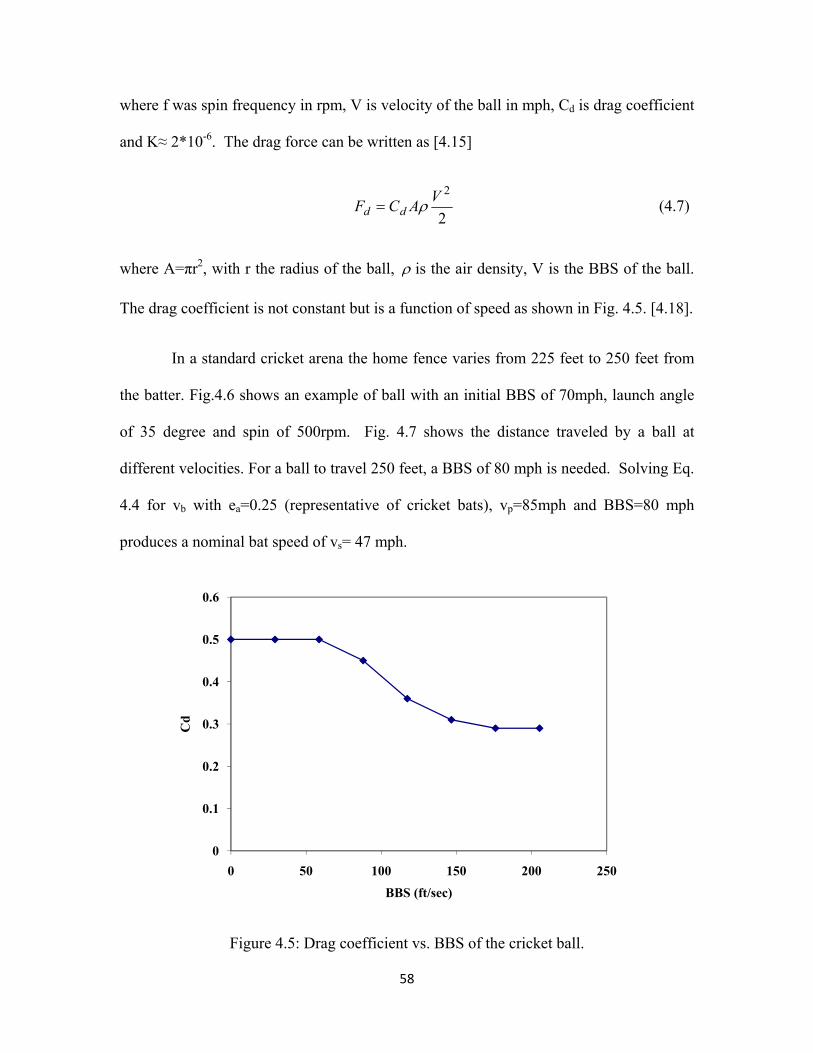
58  

where f was spin frequency in rpm, V is velocity of the ball in mph, Cd is drag coefficient

and K≈ 2*10-6. The drag force can be written as [4.15]

2

2VACF dd ρ= (4.7)

where A=πr2, with r the radius of the ball, ρ is the air density, V is the BBS of the ball.

The drag coefficient is not constant but is a function of speed as shown in Fig. 4.5. [4.18].

In a standard cricket arena the home fence varies from 225 feet to 250 feet from

the batter. Fig.4.6 shows an example of ball with an initial BBS of 70mph, launch angle

of 35 degree and spin of 500rpm. Fig. 4.7 shows the distance traveled by a ball at

different velocities. For a ball to travel 250 feet, a BBS of 80 mph is needed. Solving Eq.

4.4 for vb with ea=0.25 (representative of cricket bats), vp=85mph and BBS=80 mph

produces a nominal bat speed of vs= 47 mph.

Figure 4.5: Drag coefficient vs. BBS of the cricket ball.

0

0.1

0.2

0.3

0.4

0.5

0.6

0 50 100 150 200 250

Cd

BBS (ft/sec)

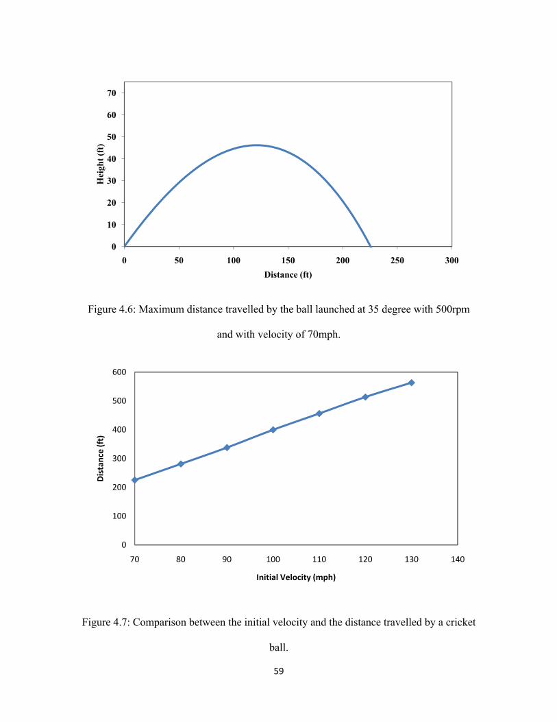
59  

Figure 4.6: Maximum distance travelled by the ball launched at 35 degree with 500rpm

and with velocity of 70mph.

Figure 4.7: Comparison between the initial velocity and the distance travelled by a cricket

ball.

0

10

20

30

40

50

60

70

0 50 100 150 200 250 300

Hei

ght (

ft)

Distance (ft)

0

100

200

300

400

500

600

70 80 90 100 110 120 130 140

Distance (ft)

Initial Velocity (mph)

60  

4.4 Test Results

Each bat was impacted six times at multiple locations along its length until a

maximum BBS location was found within 0.50 inches. A representative bat performance

curve is shown in Fig. 4.8. Note the relatively small region which produces an optimum

BBS.

Figure 4.8: Bat performance curve of E2.

4.4.1 Knock-in/oiled

A variety of treatments are applied to bats and incorporated in their design to

improve their performance. Many believe that due to the soft and fibrous nature of the

wood fibres, knock-in and oil treatment should be done to the bat before play. Knock-in

is the process of squeezing the fibres on the surface of the cricket bat by hitting the

surface with a wooden mallet or with an old ball for 2-4 hours [4.12]. The surface of the

blade is commonly knocked-in and oiled to make the bat more durable. To consider the

effect of knock-in on performance, the bats (except CS1, CS2, CSW1 and CWS2) listed

25

35

45

55

65

75

85

95

5 10 15 20 25 30

BBS (m

ph)

Pivot Position (in)

BBS

61  

in Table 4.1 were tested before and after knock-in. The process was performed by hitting

the surface of the cricket bat with a wooden mallet for 2 hours which was separated in 12

sessions of 10 minutes each.

The average BBS of the cricket bat before and after knock-in and oiling is shown

in Fig. 4.9. The maximum average BBS for the knocked bats was 0.2 mph lower than the

unknocked bats. Knock-in was observed to have a relatively small effect on performance,

decreasing it by 0.03%. Interestingly many believe that knock-in increases the stiffness

which further increases the performance of the cricket bat.

Figure 4.9: Average performance between knocked and unknocked bats.

It was interesting to compare the knock-in and oiled effect on the cricket bats

individually. For Bat E1 the peak BBS reduced by 1.97% after knock-in and oiling. Bat

E2 showed an increase of 2% in the peak BBS after knock-in and oiling.

76

77

78

79

80

81

82

83

84

19.5 20.0 20.5 21.0 21.5 22.0 22.5

BBS (m

ph)

Pivot Position (inch)

Unknocked

Knocked

62  

4.4.2 Material Comparison

The blade of most cricket bats is made of either Kashmir or English willow. Many

view English willow as superior, for which a premium price is usually paid. The average

performance of two English (E1 and E2) and Kashmir willow (K1 and K2) bats are

compared in Fig. 4.10, where the performance of English willow was observed to be

0.02% higher than Kashmir willow. There was a shift in the peak location in English

willow after knock-in.

Figure 4.10: Average performance between English willow and Kashmir willow

after knock-in and oiling.

The effect of weight on the performance can be observed by comparing the MOI

and BBS of the different cricket bats. Fig. 4.11 shows the BBS as a function of bat MOI

for English and Kashmir willow bats. It was observed that BBS increased with

increasing MOI of the bats. Both unknocked and knocked bats are included in this study.

76.0

77.0

78.0

79.0

80.0

81.0

82.0

83.0

84.0

19.5 20.0 20.5 21.0 21.5 22.0 22.5

BBS mph

Pivot Position (inch)

English 

Kashmir

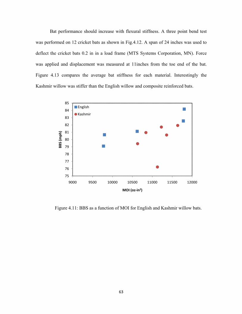
63  

Bat performance should increase with flexural stiffness. A three point bend test

was performed on 12 cricket bats as shown in Fig.4.12. A span of 24 inches was used to

deflect the cricket bats 0.2 in in a load frame (MTS Systems Corporation, MN). Force

was applied and displacement was measured at 11inches from the toe end of the bat.

Figure 4.13 compares the average bat stiffness for each material. Interestingly the

Kashmir willow was stiffer than the English willow and composite reinforced bats.

Figure 4.11: BBS as a function of MOI for English and Kashmir willow bats.

75

76

77

78

79

80

81

82

83

84

85

9000 9500 10000 10500 11000 11500 12000

BBS (m

ph)

MOI (oz‐in2)

English 

Kashmir 

64  

Figure 4.12: Cricket bat bending stiffness test.

Figure 4.13: Average stiffness results from 3-point bend tests.

The composite skin stiffens the blade and is purported to improve durability. The

performance of bats was compared with and without a composite skin. The results are

included in Fig. 4.14, which shows the skin increased the BBS by 1.44%. It should be

noted that removing the skin reduced the bat’s MOI by 4.6%. It is helpful to consider

78

78.5

79

79.5

80

80.5

81

81.5

82

82.5

83

800

850

900

950

1000

1050

1100

1150

1200

English Composite Kashmir

BBS (m

ph)

Stiffne

ss

StiffnessBBS (mph)

65  

how much of the composite skin performance was due to its added MOI. BBCOR is

insensitive to MOI and is given as,

( )vVVImQ

Vve

pBB ++=

2

(4.8)

where V , m ,v , and Ip are inbound ball speed, weight, rebound ball speed and moment of

inertia, respectively. The collision efficiency is found from ebb as

⎟⎠⎞

⎜⎝⎛

+−

=rree BB

a 1 (4.9)

where r is the bat recoil factor (Eq. 3.6). The effect of MOI on bat performance,

independent of the composite skin, may be considered in Eq. (4.4) by holding the bat-ball

COR constant and changing the bat MOI. Accordingly, a 4.5% change in MOI was found

to increase bat performance by 0.92%. Thus, roughly half of the performance advantage

attributed to a composite reinforced blade is due to its mass.

Figure 4.14: Comparison of cricket bat with and without composite skin.

77

77.5

78

78.5

79

79.5

80

80.5

81

22

BBS (m

ph)

Pivot Position (inch)

Skin

Without (With increase MOI)

66  

4.5 Summary

This study considered the performance of cricket bats. A test apparatus was

developed to measure bat properties at impact speeds representative of the play

conditions. The test method involved firing the cricket balls at various positions on a

stationary cricket bat. Bat performance has been compared using the BBS of cricket bats.

The swing speed of the cricket bat was found from the flight of the cricket ball. The MOI

of the cricket bat has a significant effect on the performance. Knock-in and oiling has a

small effect on weight, MOI and performance.

On average, the performance of English willow was observed to be 0.8% higher

than Kashmir willow. The contribution of a reinforcing composite skin to the back

surface of the bat was also relatively small (1.4%), although larger than the effect of

knock-in or willow species. It should be noted, however, that one half of this advantage

was due to the weight of the composite.

67  

References:

[4.1] Bowen, R “Cricket: a history of its growth and development throughout the world” London, Eyre and Spottiswoode, 1970.

[4.2] The laws of Cricket – 2000 Code, Marylebone Cricket Club, London, 2000 [4.3] Sayers, A. T., Koumbarakis, M., Sobey, S. “Surface Hardness of a Cricket Bat

after ‘Knock-in’”. Sports Engineering, p233-240, 2005 [4.4] Grant, C. and Nixon, S.A. “The Effect of Microstructure on the Impact

Dynamics of a Cricket Bat, Proceedings of the International Conference on the Engineering of Sport, Sheffield U.K., In Haake S. (ed.), The Engineering of Sport, Balkema, Rotterdam, p169-173, July 1996

[4.5] Stretch, R.A., Brink, A. and Hugo, J. “A Comparison of the Ball Rebound

Characteristics of Wooden and Composite Cricket Bats at Three Approach Speeds”. Sports Biomechanics Vol. 4(1) pages 37-46, 2006

[4.6] Smith, L., Broker, J., and Nathan, A. “A study of softball player swing speed”.

In A. Subic, P. Travalio, and F. Alam (Eds.), Sports dynamics: Discovery and application Melbourne, VIC: RIMT University pages 12-17 2003

[4.7] ASTM F 2398-04, Standard Test Method for Measuring Moment of Inertia

and Center of Percussion of a Baseball or Softball Bat, ASTM International 2004.

[4.8] Russell, D. “Swing Weight of a Softball bat” Submitted to The Physics

Teacher. Kettering University, Flint, MI, 2006 [4.9] Carre, M. J., James, D. M. and Haake, S. J. “Impact of a Non-homogeneous

Sphere on a Rigid Surface” Proceedings of the Institution of Mechanical Engineers; ProQuest Science Journals; 218, 3; p273, March 2004

[4.10] Penrose, T., Foster, D. and Blanksby, B. “Release Velocities of Fast Bowlers

During a Cricket Test Match” Supplement to the Australian Journal for Health, Physical Education and Recreation, p2-5, March 1976

[4.11] Smith, L., Axtell, J., T. “Mechanical Testing of Baseball Bats” Journal of

Testing and Evaluation; Vol. 31, No. 3, 2003 [4.12] Sayers, A., T., Koumbarakis, M., Sobey, S. “Surface Hardness of a Cricket

Bat After ‘Knock-in’ Sports Engineering, 8, pp 233-240; 2005

68  

[4.13] Smith, L. V., Cruz, C. M., Nathan, A. M., Russell, D. A. “How Bat Modifications Can Affect Their Response,” APCST, Tokyo, Japan, The Impact of Technology on Sport, (Subic & Ujihashi, Eds) p. 33-38 2005

[4.14] Cross, R. and Bower, R. “Effect of Swing-Weight on Swing Speed and Racket

Power”. Journal of Sports Sciences;24(1): p23-30, January 2006 [4.15] Adair, R., K. “The Physic of Baseball” Third Edition, 2002

69  

CHAPTER 5

-NUMERICAL MODEL-

5.1 Introduction

Sports such as baseball, softball, golf and tennis have benefited from research and

technology, but the game of cricket has received relatively little attention. In this study

finite element modeling was used to characterize the performance of cricket bats.

Numerical models are valuable in providing a mathematical description of high-speed

dynamic sport ball impacts [5.1].

The evaluation of cricket bat performance is nontrivial. Many factors affect the

performance of the cricket bat, such as geometry of the bat, the properties of the ball, and

the material properties of the wood. In the following study, the BBS was used to

compare bat performance from finite element models.

5.2 Ball model

5.2.1 Numerical Analysis Background

All the simulations in this work were carried out using LS-DYNA (Livermore

Software technology Corporation, Livermore, CA) Version 971. The cricket ball was

modeled as a homogenous sphere with isotropic properties. The finite element analysis

was carried out on a single 3.06Hz Intel Pentium 4 processor with 3 GB of RAM. Two

bats of same the material with different geometry were considered. The effect of a

composite skin on performance was also investigated.

70  

A dynamic finite element simulation can be performed using either implicit or

explicit time integration methods. Response is evaluated at instants separated by time

increments ∆t. At the nth time step, the equation of motion can be written as [5.3], [5.9]

                                                  [ ]{ } [ ]{ } [ ]{ } { }nnnn RDKDCDM =++ &&&                                   (5.1)

where [M], [C], [K] and Rn are the mass, damping, stiffness matrix, and the known time-

dependent forcing function at the nth instant, respectively. An explicit method assumes a

linear change in displacement over each time step. Once the displacement at tn+1 is

determined, the velocity and acceleration at time step n are approximated by central the

difference theorem as [5.3], [5.10]

( )11 }{}{21}{ −+ −Δ

= nnn DDt

D& and ( )11 }{}{2}{21}{ −+ +−Δ

= nnnn DDDt

D&& (5.2)

Equations 5.2 were be obtained from a Taylor series expansions for {D}n+1 and {D}n-1 at

time n∆t as

............}{6

}{2

}{}{}{32

1 +Δ

+Δ

+Δ+=+ nnnnn DtDtDtDD &&&&&& (5.2.a)

............}{6

}{2

}{}{}{32

1 +Δ

+Δ

+Δ+=− nnnnn DtDtDtDD &&&&&& (5.2.b)

Subtracting Eq. (5.2b) from Eq. (5.2a) yields Eq. 5.2,. In both cases, the high

order terms are discarded. Substitution of Eqs. (5.2) into Eq. 5.1 yields [5.10]

122 21

)(1

)(2)( −⎥

⎦

⎤⎢⎣

⎡Δ

−Δ

−⎥⎦

⎤⎢⎣

⎡Δ

−−= nn DCMt

DMt

KRtF (5.2.c)

71  

where, if linear conditions prevail, F(t)=ADn+1. Thus for any n, Dn+1 is calculated from

values of Dn and Dn-1.

An implicit integration method assumes a constant average acceleration over each

time step, between tn and tn+1. The equation of motion is evaluated and the resulting

accelerations are used to obtain the velocities displacements at tn+1 as [5.3],

[ ]nnnn DDtDD }){1(}{}{}{ 11&&&&&& γγ −+Δ+= ++ (5.3.a)

[ ]nnnnn DDtDtDD }){21(}{221}{}{}{ 1

21

&&&&& ββ −+Δ+Δ+= ++ (5.3.b)

where the numerical factors γ and β control the numerical accuracy, stability, and

damping Substituting Eqs. 5.3.a and 5.3.b in Eq.5.1 we obtain

Mt

Ct

KA 2)(1Δ

+Δ

+=ββ

γ (5.3.c)

),,,,,,,,()( nnn DDDMCRtfftF &&&Δ= β (5.3.d)

The complete expression is not written because it’s lengthy and not essential to our

discussion. Using Eqs. 5.3.c and 5.3.d, 1+nD&& is calculated from Dn, nD& , and nD&& .  

An other difference between the two techniquies is that in the explicit method the

coefficient matrix of {D}n+1 can be made diagonal, so that {D}n+1 is cheaply inverted for

each time step. In the implicit method, {D}n+1 cannot be made diagonal, so that cost per

step is greater [5.3]. Neither an implicit nor explicit solution is perfect in all cases. In the

present study the implicit time integration method was used.  

72  

The cricket ball was represented as a solid isotropic sphere of radius 1.41 inches

and 5.65oz. A viscoelastic material model (*MAT_006) consisting of 3584 eight node

solid elements was selected for the cricket ball, defined by the time dependent shear

modulus [5.2], [5.3], [5.4] as,

( ) ( )teGGGtG β−∞∞ −+= 0)( (5.4)

and a constant bulk modulus, k where G0 is the instantaneous shear modulus G∞ is the

long shear modulus, and β determines the time sensitivity of the model. The short term

modulus is dominant near t=0, while near t= ∞ the long term modulus is dominant. The

decay constant β determines the rate at which the long term modulus dominates the

material response. The cricket ball can be tuned for COR and dynamic stiffness by

adjusting one or more of the material properties.

Linear viscoelasticity was assumed for the deviatoric stress tensor, which was

calculated from the Jaumann rate integral (also known as the hereditary integral) [5.5] as

( ) ( )∫ −=t

ijij dDtG0

'' 2ˆ τττσ (5.5)

where the prime denotes the deviatoric part of the stress rate, ^

ijσ ′ , the strain rate 'ijD and

τ is time. A recursion formula was used to compute the new value of the Jaumann

integral at time tn+1 from its value at tn [5.5].

The dynamic stiffness apparatus was modeled numerically as shown in Fig. 5.1.

The rebound speed was obtained using the *DATABASE_NODOUT ASCII command.

To remove the effect of vibration within the ball after the impact, the center node of the

73  

ball was chosen for the rebound speed. Fig.5.2 shows the velocity vs. time data obtained

from the *DATABASE_NODOUT ASCII file.

Figure 5.1: Dynamic stiffness apparatus modeled in LS-DYNA.

Figure 5.2: A plot of ball speed vs. time.

-600-400-200

0200400600800

10001200

0.0000 0.0002 0.0004 0.0006 0.0008 0.0010

Bal

l Spe

ed (i

n/s)

Time (sec)

74  

In Fig. 5.2, the initially positive flat line signifies the speed of the ball before

impact whereas the negative flat line represents the speed of the ball after impact with the

flat steel plate. The slope between the flat lines corresponds to the compression and

expansion phases of the cricket ball. A force was generated when the cricket ball

contacted the flat rigid plate. The *DATABASE_RCFORCE ASCII command was used

to output the impact force as shown in Fig. 5.3. The ball was impacted at the flat rigid

plate at 60mph. Table 5.2 summarizes the viscoelastic properties used for the cricket ball

in Fig. 5.1 and 5.3:

Table 5.1: Viscoelastic properties of cricket ball used in following figures

Mass Density (lbs2/in4)

Shear Modulus Short Time(G0)

(psi)

Shear Modulus Long time (G∞)

(psi) Beta (β)

Elastic Bulk Modulus(K)

(psi) 7.96E-05 6300 1667 10500 1.950e4

Figure 5.3: Force vs. time plot coarse.

0

500

1000

1500

2000

2500

3000

3500

4000

0.0000 0.0005 0.0010 0.0015

Y-F

orce

(lbs

)

Time (sec)

75  

5.2.2 Model Tuning with Experimental Results

A refined cricket model with accurate material properties is necessary to simulate

the measured behavior of the cricket ball. Impact simulations are often run with a coarse

mesh refinement to reduce solution time.

The standard mesh of the cricket ball consisted of 3584, 8-noded solid elements

whereas the fine mesh consisted of 12096, 8-noded solid elements. Fig. 5.4 shows the

fine cricket ball mesh. The rigid plate was modeled with dimensions 4 x 1.5 x 2.25 inches

using 6336 8-noded solid elements (*ELEMENT_SOLID) and the properties of steel. All

nodes on the back side of the rigid plate were constrained to simulate a rigid boundary

condition. A contact card (*CONTACT_SURFACE_TO_SURFACE) was used between

the cricket ball and steel plate to prevent penetration during impact. The stationary plate

was defined as master, and the cricket ball was the slave segment.

The explicit solution was obtained through loops, where the loop time steps were

based upon the relative stiffness of the contacting surface. The initial velocity was

applied to all the nodes of the cricket ball model, so that every node was given the same

initial velocity. The initial velocity of the cricket ball for the finite model was 60mph.

The velocity card (*INTIAL VELOCITY) was used to apply the initial velocity to cricket

ball. The computational time required to run the standard mesh was 7 minutes, while the

fine mesh required approximately 15 minutes. It was observed from the results that the

COR and dynamic compression of the fine mesh was 1.8% and 1.0%, respectively higher

than the standard mesh. Due to an increased number of elements the force vs. time curve

became smoother in the fine mesh as shown in Fig. 5.5.

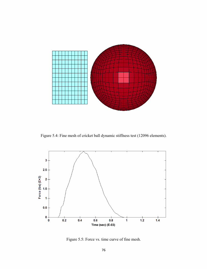
76  

Figure 5.4: Fine mesh of cricket ball dynamic stiffness test (12096 elements).

Figure 5.5: Force vs. time curve of fine mesh.

77  

The linear viscoelastic element allows the user to model discrete material

properties [5.5]. The viscoelastic properties were adjusted until a good agreement was

achieved between the experimental and finite element models. Several parameters have

been used in softball and baseball studies in past, as shown in Table 5.2. Fig. 5.6 shows

the comparison of finite element and experimental results of cricket ball impacting a load

cell at 60mph. Good agreement can be seen between the finite element and experiment.

Table 5.2: Viscoelastic parameter values of Softball and Baseball [5.4]

Model k (Pa) G0 (pa) G∞ (Pa) β (Hz)

Baseball 27.57x109 1.689x106 5.86x106 850

Softball 27.57x109 861.8x103 3.102x106 950

Rubber Baseball 19.0x106 2.0x106 1.0x106 1.25x103

Figure 5.6: Comparison of finite element and experiment of cricket ball impacting a load

cell at vb =60mph (26.8 m/s).

0

500

1000

1500

2000

2500

3000

3500

4000

0.0000 0.0002 0.0004 0.0006 0.0008 0.0010

Forc

e (lb

)

Time (sec)

FEM Cricket ball

G0 = 6300 psiGi = 1667 psiβ = 10500k = 19500 psi

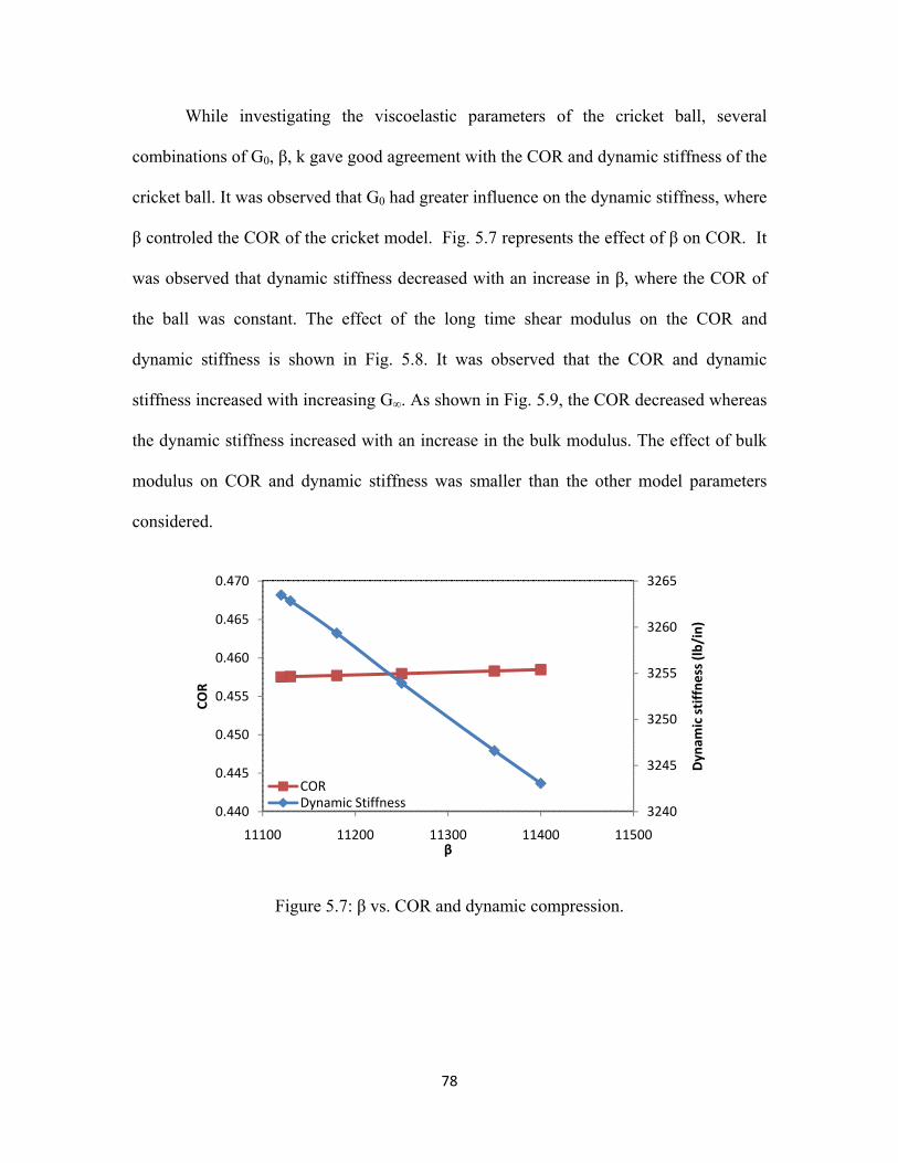
78  

While investigating the viscoelastic parameters of the cricket ball, several

combinations of G0, β, k gave good agreement with the COR and dynamic stiffness of the

cricket ball. It was observed that G0 had greater influence on the dynamic stiffness, where

β controled the COR of the cricket model. Fig. 5.7 represents the effect of β on COR. It

was observed that dynamic stiffness decreased with an increase in β, where the COR of

the ball was constant. The effect of the long time shear modulus on the COR and

dynamic stiffness is shown in Fig. 5.8. It was observed that the COR and dynamic

stiffness increased with increasing G∞. As shown in Fig. 5.9, the COR decreased whereas

the dynamic stiffness increased with an increase in the bulk modulus. The effect of bulk

modulus on COR and dynamic stiffness was smaller than the other model parameters

considered.

Figure 5.7: β vs. COR and dynamic compression.

3240

3245

3250

3255

3260

3265

0.440

0.445

0.450

0.455

0.460

0.465

0.470

11100 11200 11300 11400 11500

Dynam

ic stiffne

ss (lb/in)

COR

β

CORDynamic Stiffness

79  

Figure 5.8: Long time shear modulus Gi vs. COR and dynamic compression.

Figure 5.9: Bulk modulus (k) vs. COR and dynamic compression.

2910

2915

2920

2925

2930

2935

2940

2945

2950

0.480

0.484

0.488

0.492

0.496

0.500

0.504

0.508

1580 1600 1620 1640 1660 1680

Dynam

ic com

pression

 (lbs)

COR

G∞ (psi)

CORDynamic compression

3310

3315

3320

3325

3330

3335

3340

3345

3350

3355

0.449

0.454

0.459

0.464

0.469

0.474

0.479

0.484

1.30E+04 1.35E+04 1.40E+04 1.45E+04 1.50E+04 1.55E+04

Dynam

ic com

pression

 (lbs)

COR

K (psi)

CORDynamic compression

80  

5.2.3 Rate Dependence

The finite element model showed good agreement with experimental data over a

range of inbound speeds. Fig. 5.10 compares the force-displacement between the finite

element model and experiment for ball model Bb. Fig. 5.11 and 5.12 show compare the

COR and dynamic stiffness of the finite element model with experimental data as a

function of speed. The general trend of COR decreasing with increasing speed was

observed for both finite model and experimental data. The experimental COR had steeper

curve than finite element model. This occurred for all combinations of material

parameters considered. The dynamic stiffness vs. speed of the finite element model and

experimental data showed good agreement.

Figure 5.10: Representative force-displacement curve of Bb for experiment and FEM

model.

0

1000

2000

3000

4000

5000

6000

7000

0 0.1 0.2 0.3 0.4 0.5

Force (lb

s)

Displacement (in)

Ball Bb

FEM Model

81  

Figure 5.11: Comparison of COR between average of dozen balls and FEA model as a

function of incoming speed.

Figure 5.12: Comparison of the dynamic stiffness between the average of 12 balls and

FEA model as a function of incoming speed.

0.430

0.440

0.450

0.460

0.470

0.480

0.490

0.500

55 60 65 70 75 80 85

CO

R

ExpFEA

30003250350037504000425045004750500052505500

55 60 65 70 75 80 85

Dyn

amic

Stif

fnes

s (lb

/in)

ExpFEA

82  

5.3 Bat model

5.3.1 Numerical Model

The geometry of each bat model was developed using CATIA Version 5 Revision

17. The geometry of the cricket bat is not simple; it is flat in the blades region and tapers

into a cylindrical handle. Two types of coordinate measuring machines (CMM) were

used to measure the bat profile (Phytom model and CMM model). The surfaces created

from these techniques were irregular, however. Instead, the primary dimensions of the

blade and handle were measured and smooth curves were fit to these points to create the

surface.

The upper surface of the cricket ball was the slave segment and the lower surface

of the cricket bat was the master segment. A surface-to-surface contact algorithm

between the bat and ball was used due to the complicated deformation that typically

occurs during an explicit dynamic analysis. The mass density of the cricket ball was kept

constant at 7.96 x10-5 lbs2/in4 to provide a ball weight of 5.65 oz. To improve correlation

with the measured bat performance β was adjusted as shown in Table 5.3.

Table 5.3: Values of Viscoelastic properties used in the study for Bat-tuned model

Mass Density (lbs2/in4)

Shear Modulus Short Time(G0) (psi)

Shear Modulus Long time (Gi)

(psi) Beta (β)

Elastic Bulk Modulus(K)

(psi) 7.96E-05 6300 1667 10500 1.95E+04

83  

5.3.2 Bat Models and Materials

Two cricket bat designs were modeled in this study, a traditional design (M1), and

a faceted design (M2) as shown in Fig. 5.13 and 5.14. Wood is an orthotropic material,

thus its properties in the longitudinal, radial and transverse directions are different.

Figure 5.13: Traditional design (M1) Bat model.

84  

Figure 5.14: Faceted design (M2) bat model.

Wood is a natural material and its density varies from species to species. The

density of willow and cane varies from 4.24x10-4 lbs2/in4 to 7.018 x10-5 lbs2/in4 [5.8],

and 6.74 x10-5 lbs2/in4 – 4.29x10-5 lbs2/in4 [5.9], respectively. The density of the willow

and cane were tailored to match the measured weight and mass moment of inertia (MOI)

of the bat. Willow and cane elastic properties are summarized in Table 5.5. The elastic

properties of the cane handle have a small effect on bat performance. The transverse

properties of the handle are even less important. For this reason, and since the orthotropic

properties of cane are not known, it was assumed to be isotropic.

Table 5.4: Values of Viscoelastic properties used in the study for Bat-tuned model

Mass Density (lbs2/in4) 

Shear Modulus Short Time(G0) (psi) 

Shear Modulus Long time (G∞) (psi) 

Beta (β) Elastic Bulk Modulus(K) 

(psi) 

7.89E‐05  4750  1667  10500  1.95E+04 

85  

Table 5.5: Elastic Properties of Cricket Bat (Coordinate system as in Fig. 5.14 and 5.15)

Young’s Modulus (Msi)

Mass Density (lbs2/in4)

Shear Modulus (Msi) Poisson’s ratio

Ex Ey Ez ρ0 Gxy Gyz Gzx νyx νzx νzy

Willow 0.479 0.0319 0.255 4.14x10-5 0.0479 0.00479 0.0479 0.015 0.16 0.6

Cane 0.318 0.318 0.318 4.66x10-5 - - - 0.3 0.3 0.3

Figure 5.15: Principal axis of wood.

The composite skin was modeled using the properties of carbon epoxy AS4/3501-

6 with a [0/90]s layup of thickness 0.02 inches. The laminated properties of the composite

skin are presented in Table 5.6.

86  

Table 5.6: Laminated [0/90]s Properties of Composite Skin

Young’s Modulus (Msi)

Mass Density (lbs2/in4)

Shear Modulus (Msi) Poisson’s ratio

Ex Ey Ez ρ0 Gxy Gyz Gzx νyx νzx νzy

Composite 11.1 11.1 1.14 1.55x10-4 1.04 0.912 0.912 0.037 0.0158 0.26

5.3.3 Modeling the Bat-Ball Impact

The *BOUNDARY_SPC_NODE_ID card was used to constrain the nodes at the

pivot point. A termination time of 0.003s was used to allow for initial ball motion, the

bat-ball impact period and the rebound ball motion.

A comparison between the experiment and FEA length and mass properties is

given in Table 5.7 and 5.8. The mass properties of the bat with and without the

composite skin are compared in Table 5.8.

Table 5.7: Comparison of measured and modeled M1 bat properties

Length (in) Weight (oz) MOI (oz-in2)

Experimental 33.54 37.68 9799

FE Model 33.54 37.68 9779

% Difference 0.000 0.000 0.199

 

 

 

87  

Table 5.8: Comparison of measured and modeled M2 bat properties

Length (in) Weight (oz) MOI (oz-in2)

Experimental 34.92 39.54 11778

FE Model 34.92 41.9 11711

% Difference 0.000 -5.6 0.579

5.4 Experimental Comparison

The elastic properties of the wood can vary within the same species. A study was

conducted to consider the effect of elastic properties in each direction independently on

bat performance. When the radial modulus was doubled, the BBS increased by 1%.

While the BBS increased by 2% when the tangential modulus was doubled. It was also

observed that there was 10% increase in BBS when the longitudinal modulus was

doubled.

The performance of the M1 model is shown in Figure 5.16. The model shows good

agreement with the experiment. Model M2 is compared with experiment over an

extended impact location range in Fig. 5.17. Note the relatively small region which

produces a maximum BBS.

88  

Figure 5.16: Experimental validation of the M1 model at different impact locations.

Figure 5.17: Representative performance curves for bat and model.

72

72.5

73

73.5

74

74.5

75

19.5 20 20.5 21 21.5 22 22.5

BB

S (m

ph)

Impact Location (inch)

FEA

Exp

25

30

35

40

45

50

55

60

65

70

75

80

85

8 9 10 11 12 13 14 15 16 17 18 19 20 21 22 23 24 25 26

BB

S (m

ph)

Impact Location (in)

Exp

FEA

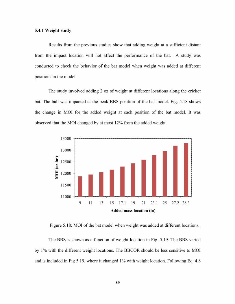
89  

5.4.1 Weight study

Results from the previous studies show that adding weight at a sufficient distant

from the impact location will not affect the performance of the bat. A study was

conducted to check the behavior of the bat model when weight was added at different

positions in the model.

The study involved adding 2 oz of weight at different locations along the cricket

bat. The ball was impacted at the peak BBS position of the bat model. Fig. 5.18 shows

the change in MOI for the added weight at each position of the bat model. It was

observed that the MOI changed by at most 12% from the added weight.

Figure 5.18: MOI of the bat model when weight was added at different locations.

The BBS is shown as a function of weight location in Fig. 5.19. The BBS varied

by 1% with the different weight locations. The BBCOR should be less sensitive to MOI

and is included in Fig 5.19, where it changed 1% with weight location. Following Eq. 4.8

11000

11500

12000

12500

13000

13500

9 11 13 15 17.1 19 21 23.1 25 27.2 28.3

MO

I (oz

-in2 )

Added mass location (in)

90  

the BBCOR is independent of inbound speed and the mass of the bat, so the BBCOR

should be consistent with the change in MOI by adding mass at different locations.

Figure 5.19: BBCOR as a function of weight location from the pivot.

5.4.2 Composite Skin

The mass properties of two bats with and without a skin are compared in Table

5.9. The performance of a bat was compared with and without a composite skin, as

shown in Fig. 5.20. The effect of the 0.02 inch thick composite skin was considered in

the numeric model using the properties of Table 5.8. The results are included in Fig. 5.20

and 5.21, where the skin increased the BBS by 2.2%. The FEA model had a different

geometry than was tested experimentally. Therefore, the MOI of the FEA model was

reduced to match the experimentally tested bat. A composite skin weighting 1.6 oz was

considered in the numeric study; taken as average of the two composite bats tested.

0.525

0.53

0.535

0.54

0.545

0.55

0.555

0.56

0.565

0.57

75

75.5

76

76.5

77

77.5

78

78.5

8 10 12 14 16 18 20 22 24 26 28 30

BBCO

R

BBS

Mass Position

BBS

BBCOR

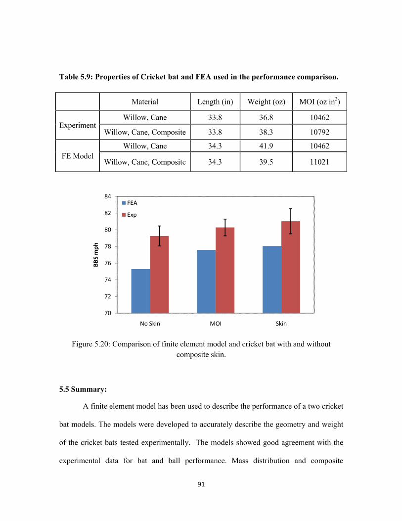
91  

Table 5.9: Properties of Cricket bat and FEA used in the performance comparison.

 

Figure 5.20: Comparison of finite element model and cricket bat with and without composite skin. 

 

5.5 Summary:

A finite element model has been used to describe the performance of a two cricket

bat models. The models were developed to accurately describe the geometry and weight

of the cricket bats tested experimentally. The models showed good agreement with the

experimental data for bat and ball performance. Mass distribution and composite

70

72

74

76

78

80

82

84

No Skin MOI Skin

BBS mph

FEA

Exp

Material Length (in) Weight (oz) MOI (oz in2)

Experiment Willow, Cane 33.8 36.8 10462

Willow, Cane, Composite 33.8 38.3 10792

FE Model Willow, Cane 34.3 41.9 10462

Willow, Cane, Composite 34.3 39.5 11021

92  

reinforcement were shown to have a measurable effect on bat performance. In

comparison with hollow baseball and softball bats, however, the effect was relatively

small.

93  

References:

[5.1] Nicolls, R.L., Miller, K., and Elliott, B.C. “Modeling Deformation Behavior of

the Baseball” Journal of Applied Biomechanics. pp: 18-30. 2005.

[5.2] Mustone, T.J., Sherwood, J.A “Using Ls-Dyna to Characterize the Performance of

Baseball Bats” 5th International Ls-Dyna Users Conference, South-field, MI.

Livermore, CA: Livermore Software Technology Corp. pp: 21-22, Sept. 1998.

[5.3] Cook, D.R. “Concepts And Applications Of Finite Element Analysis” Fourth

Edition.

[5.4] Smith, L.V, Shenoy, M.M., Axtell, J.T. “Performance assessment of wood, metal

and composite baseball bats”. ASME IMECE, 2000

[5.5] LS-DYNA Keyword Users Manual. Liversome Software Technology

Corporation. August 2007. Version 971

[5.6] Biesen, E. D., “Prediction of plastic Deformation in Aluminum Softball Bats

Using Finite Element Analysis” Washington State University. August 2006.

[5.7] Penrose. J. M. T., Hose, D. R. “Finite Element Impact Analysis of a Flexible

Cricket Bat for Design Optimization” The Engineering of Sports. 1998

[5.8] Khanduri, A.K., Shukla, N.K. “Physical and Mechanical Properties of Salix Alba-

An Assessment” J. Timb. Dev. Assoc. (India) Vol. XLIV. Nov 4, October 1998

[5.9] Barizan, R. S. R., Aswad, R.M. “Cane Properties of Cultivated Rotan Manau

under Second Growth Forests: Relations Between Maturity and Strength”

Highlights of FRIM’s IRPA projects. Pp. 186-191. 2005.

[5.10] Cook, R.D. “Finite Element Modeling for Stess Analysis” John Wiley and Sons,

Inc.

94  

CHAPTER 6

-SUMMARY-

6.1 Review

The study measured and compared the performance of different models of cricket

balls and bats. The following summarizes the major findings of this work.

6.2 Ball Testing

A high-speed canon was used to measure the dynamic properties of cricket balls

by impacting a rigid wall at 60 – 80mph. The COR of all the cricket balls decreased with

increasing impact speed. Seam impacts had a higher COR and dynamic stiffness than a

face impacts. A gradual increase in displacement and force with impact speed was

observed in both seam and face impacts. The relationship between the peak force and

impact speed was non-linear. The ball model with a rubber core had lower COR and

variation than the ball model which contained a cork core.

6.3 Bat Testing

A test apparatus was developed to measure bat properties at impact speeds

representative of the play conditions. The test method involved firing the cricket balls at

various positions on a stationary cricket bat. A bat performance measure was derived in

terms of an ideal batted-ball speed based on play conditions. The swing speed of the

cricket bat was found from the flight of the cricket ball. The MOI of the cricket bat had a

measureable effect on bat performance. Knock-in and oiling had a smaller effect that

weight or MOI on performance.

95  

Wood species had a relatively small effect where the performance of English

willow bats was on average 0.84% higher than Kashmir willow bats. The contribution of

a reinforcing composite skin to the back surface of the bat was also relatively small

(1.4%), although larger than the effect of knock-in or willow species. It should be noted,

however, that one half of this advantage was due to the weight of the composite. While

the different treatments and designs had a measurable effect on performance, they were

much smaller than the 10% difference observed between solid wood and hollow baseball

and softball bats.

6.4 Numeric model

A dynamic finite element model was employed to simulate the bat-ball impact.

The ball was modeled as a linear viscoelastic material which provided the mechanism of

energy loss during impact. The ball model was tuned by adjusting its material properties

to match its measurable response. The model showed good agreement with the

experimental data for bat and ball performance. Mass distribution and composite

reinforcement were shown to have a measurable effect on bat performance. In

comparison with hollow baseball and softball bats, however, the effect was relatively

small.

6.5 Future work

The work performed here was successful to answer many questions related to the

performance of cricket bats. However, there are many issues deserving for further

investigation.

96  

It was shown that cricket balls had a significant effect on the performance of

cricket bats. For changes to be implemented, additional data of COR and dynamic

stiffness at several speeds is needed. More investigation is needed on seam and face

impacts.

Another area of research is numeric modeling. Refinement of the mesh density

need to be further investigated. Another area that needs to be addressed is the orthotropic

properties of willow.

97  

APPENDIX ONE

Detailed information used for cricket bat model with composite skin

*KEYWORD *TITLE $# title LS-DYNA keyword deck by LS-PRE *CONTROL_TERMINATION $# endtim endcyc dtmin endeng endmas 0.002000 *DATABASE_ELOUT $# dt binary 1.0000X10-4 1 *DATABASE_NODOUT $# dt binary 1.0000X10-5 1 *DATABASE_RCFORC $# dt binary 1.0000X10-5 1 *DATABASE_BINARY_D3PLOT $# dt lcdt beam npltc 1.0000X10-4 $# ioopt 0 *DATABASE_HISTORY_NODE $# id1 id2 id3 id4 id5 id6 id7 id8 57685 6059 6072 57604 *BOUNDARY_SPC_NODE $# nid cid dofx dofy dofz dofrx dofry dofrz 14151 0 0 1 1 14268 0 0 1 1 14385 0 0 1 1 14502 0 0 1 1 14619 0 0 1 1 14736 0 0 1 1 14853 0 0 1 1 14970 0 0 1 1 15087 0 0 1 1 15204 0 0 1 1 15321 0 0 1 1 15438 0 0 1 1 15555 0 0 1 1 15672 0 0 1 1 15789 0 0 1 1 15906 0 0 1 1 16023 0 0 1 1 *CONTACT_SURFACE_TO_SURFACE_ID $# cid title 1 $# ssid msid sstyp mstyp sboxid mboxid spr mpr 2 1

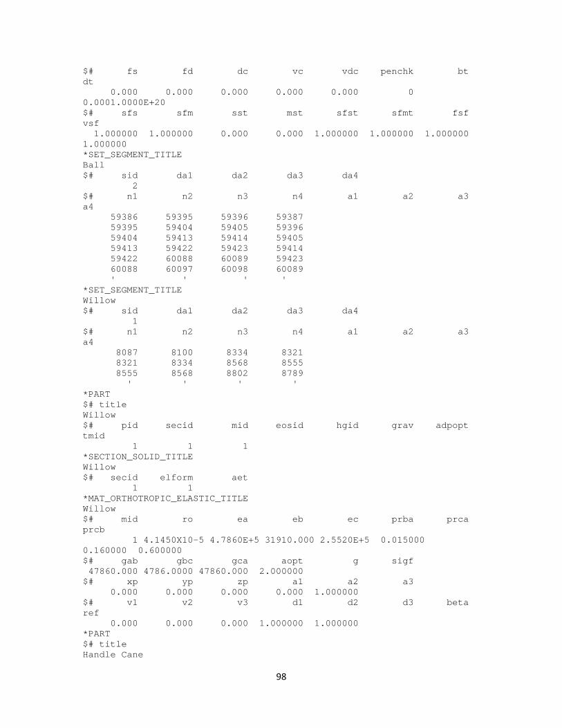
98  

$# fs fd dc vc vdc penchk bt dt 0.000 0.000 0.000 0.000 0.000 0 0.0001.0000E+20 $# sfs sfm sst mst sfst sfmt fsf vsf 1.000000 1.000000 0.000 0.000 1.000000 1.000000 1.000000 1.000000 *SET_SEGMENT_TITLE Ball $# sid da1 da2 da3 da4 2 $# n1 n2 n3 n4 a1 a2 a3 a4 59386 59395 59396 59387 59395 59404 59405 59396 59404 59413 59414 59405 59413 59422 59423 59414 59422 60088 60089 59423 60088 60097 60098 60089 ' ' ' ' *SET_SEGMENT_TITLE Willow $# sid da1 da2 da3 da4 1 $# n1 n2 n3 n4 a1 a2 a3 a4 8087 8100 8334 8321 8321 8334 8568 8555 8555 8568 8802 8789 ' ' ' ' *PART $# title Willow $# pid secid mid eosid hgid grav adpopt tmid 1 1 1 *SECTION_SOLID_TITLE Willow $# secid elform aet 1 1 *MAT_ORTHOTROPIC_ELASTIC_TITLE Willow $# mid ro ea eb ec prba prca prcb 1 4.1450X10-5 4.7860E+5 31910.000 2.5520E+5 0.015000 0.160000 0.600000 $# gab gbc gca aopt g sigf 47860.000 4786.0000 47860.000 2.000000 $# xp yp zp a1 a2 a3 0.000 0.000 0.000 0.000 1.000000 $# v1 v2 v3 d1 d2 d3 beta ref 0.000 0.000 0.000 1.000000 1.000000 *PART $# title Handle Cane

99  

$# pid secid mid eosid hgid grav adpopt tmid 2 2 2 *SECTION_SOLID_TITLE Handle Cane $# secid elform aet 2 1 *MAT_ELASTIC_TITLE Handle Cane $# mid ro e pr da db not used 2 4.6790X10-5 1.5910E+5 0.300000 *PART $# title Ball $# pid secid mid eosid hgid grav adpopt tmid 3 3 3 *SECTION_SOLID_TITLE Ball $# secid elform aet 3 1 *MAT_VISCOELASTIC_TITLE Ball $# mid ro bulk g0 gi beta 3 7.9600X10-5 19500.000 4750.0000 1667.0000 10500.000 *PART $# title Composite Skin $# pid secid mid eosid hgid grav adpopt tmid 4 4 4 *SECTION_SHELL_TITLE Composite Skin $# secid elform shrf nip propt qr/irid icomp setyp 4 2 1.000000 2 1 0 0 1 $# t1 t2 t3 t4 nloc marea idof edgset 0.025000 0.025000 0.025000 0.025000 *MAT_ORTHOTROPIC_ELASTIC_TITLE Composite skin $# mid ro ea eb ec prba prca prcb 4 5.5400X10-5 1.1090E+7 1.1090E+7 1.1430E+6 0.037000 0.015800 0.260000 $# gab gbc gca aopt g sigf 1.0400E+6 9.1190E+5 9.1190E+5 2.000000 $# xp yp zp a1 a2 a3 0.000 0.000 0.000 0.000 1.000000 $# v1 v2 v3 d1 d2 d3 beta ref 0.000 0.000 0.000 1.000000 1.000000 *INITIAL_VELOCITY $# nsid nsidex boxid irigid 3 $# vx vy vz vxr vyr vzr

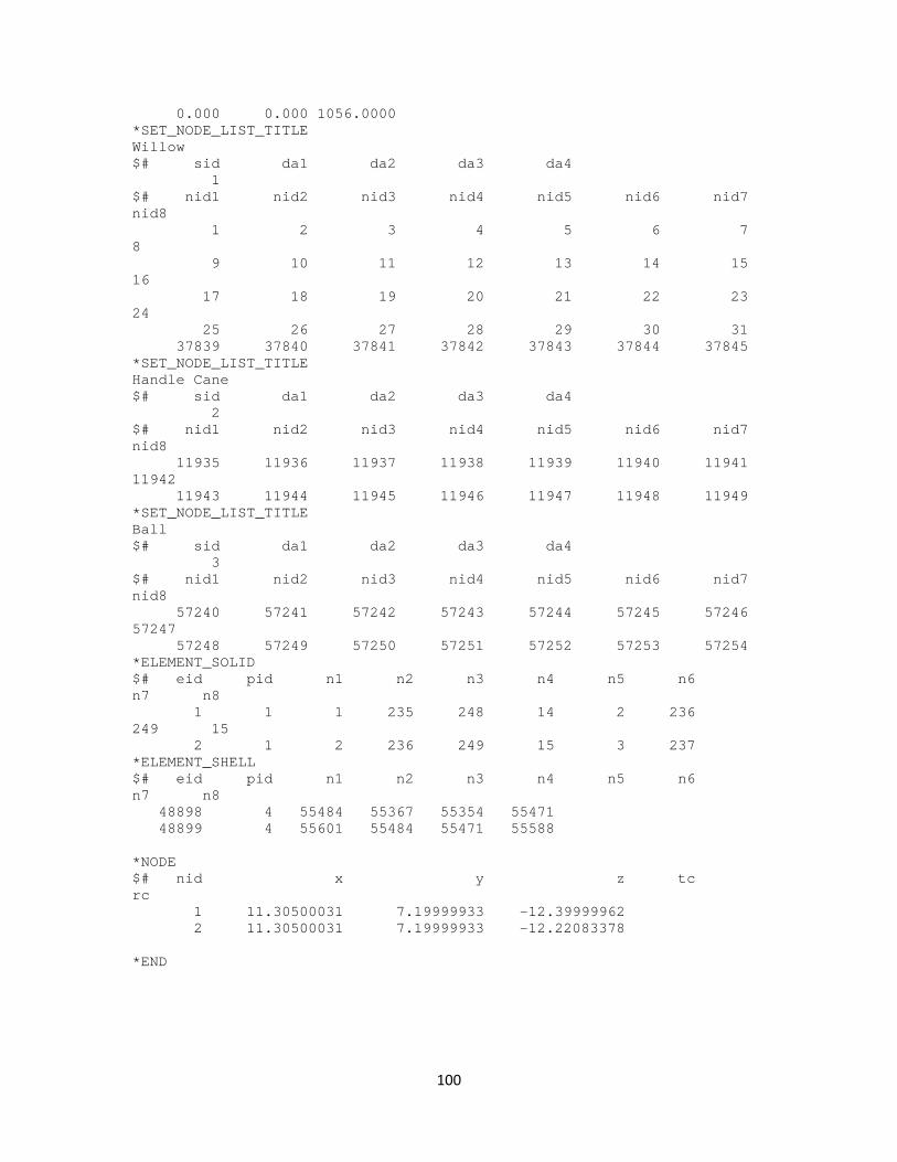
100  

0.000 0.000 1056.0000 *SET_NODE_LIST_TITLE Willow $# sid da1 da2 da3 da4 1 $# nid1 nid2 nid3 nid4 nid5 nid6 nid7 nid8 1 2 3 4 5 6 7 8 9 10 11 12 13 14 15 16 17 18 19 20 21 22 23 24 25 26 27 28 29 30 31 37839 37840 37841 37842 37843 37844 37845 *SET_NODE_LIST_TITLE Handle Cane $# sid da1 da2 da3 da4 2 $# nid1 nid2 nid3 nid4 nid5 nid6 nid7 nid8 11935 11936 11937 11938 11939 11940 11941 11942 11943 11944 11945 11946 11947 11948 11949 *SET_NODE_LIST_TITLE Ball $# sid da1 da2 da3 da4 3 $# nid1 nid2 nid3 nid4 nid5 nid6 nid7 nid8 57240 57241 57242 57243 57244 57245 57246 57247 57248 57249 57250 57251 57252 57253 57254 *ELEMENT_SOLID $# eid pid n1 n2 n3 n4 n5 n6 n7 n8 1 1 1 235 248 14 2 236 249 15 2 1 2 236 249 15 3 237 *ELEMENT_SHELL $# eid pid n1 n2 n3 n4 n5 n6 n7 n8 48898 4 55484 55367 55354 55471 48899 4 55601 55484 55471 55588 *NODE $# nid x y z tc rc 1 11.30500031 7.19999933 -12.39999962 2 11.30500031 7.19999933 -12.22083378 *END  

101  

APPENDIX TWO

Detailed information used for cricket bat model in weight study

*KEYWORD *TITLE $# title LS-DYNA keyword deck by LS-PRE *CONTROL_TERMINATION $# endtim endcyc dtmin endeng endmas 0.002500 *DATABASE_ELOUT $# dt binary 1.0000X10-4 1 *DATABASE_NODOUT $# dt binary 1.0000X10-5 1 *DATABASE_RCFORC $# dt binary 1.0000X10-5 1 *DATABASE_BINARY_D3PLOT $# dt lcdt beam npltc 1.0000X10-4 $# ioopt 0 *DATABASE_HISTORY_NODE $# id1 id2 id3 id4 id5 id6 id7 id8 57685 6059 6072 57604 *BOUNDARY_SPC_NODE $# nid cid dofx dofy dofz dofrx dofry dofrz 14151 0 0 1 1 14268 0 0 1 1 14385 0 0 1 1 *CONTACT_SURFACE_TO_SURFACE_ID $# cid title 1 $# ssid msid sstyp mstyp sboxid mboxid spr mpr 2 1 $# fs fd dc vc vdc penchk bt dt 0.000 0.000 0.000 0.000 0.000 0 0.0001.0000E+20 $# sfs sfm sst mst sfst sfmt fsf vsf 1.000000 1.000000 0.000 0.000 1.000000 1.000000 1.000000 1.000000 *SET_SEGMENT_TITLE Ball $# sid da1 da2 da3 da4

102  

2 $# n1 n2 n3 n4 a1 a2 a3 a4 59386 59395 59396 59387 *SET_SEGMENT_TITLE Willow $# sid da1 da2 da3 da4 1 $# n1 n2 n3 n4 a1 a2 a3 a4 8087 8100 8334 8321 8321 8334 8568 8555 *PART $# title Willow $# pid secid mid eosid hgid grav adpopt tmid 1 1 1 *SECTION_SOLID_TITLE Willow $# secid elform aet 1 1 *MAT_ORTHOTROPIC_ELASTIC_TITLE Willow $# mid ro ea eb ec prba prca prcb 1 4.1450X10-5 4.7860E+5 31910.000 2.5520E+5 0.015000 0.160000 0.600000 $# gab gbc gca aopt g sigf 47860.000 4786.0000 47860.000 2.000000 $# xp yp zp a1 a2 a3 0.000 0.000 0.000 0.000 1.000000 $# v1 v2 v3 d1 d2 d3 beta ref 0.000 0.000 0.000 1.000000 1.000000 *PART $# title Handle Cane $# pid secid mid eosid hgid grav adpopt tmid 2 2 2 *SECTION_SOLID_TITLE Handle Cane $# secid elform aet 2 1 *MAT_ELASTIC_TITLE Handle Cane $# mid ro e pr da db not used 2 4.6790X10-5 1.5910E+5 0.300000 *PART $# title Ball $# pid secid mid eosid hgid grav adpopt tmid 3 3 3

103  

*SECTION_SOLID_TITLE Ball $# secid elform aet 3 1 *MAT_VISCOELASTIC_TITLE Ball $# mid ro bulk g0 gi beta 3 7.9600X10-5 19500.000 4750.0000 1667.0000 10500.000 *INITIAL_VELOCITY $# nsid nsidex boxid irigid 3 $# vx vy vz vxr vyr vzr 0.000 0.000 1056.0000 *SET_NODE_LIST_TITLE Willow $# sid da1 da2 da3 da4 1 $# nid1 nid2 nid3 nid4 nid5 nid6 nid7 nid8 1 2 3 4 5 6 7 8 9 10 11 12 13 14 15 *SET_NODE_LIST_TITLE Ball $# sid da1 da2 da3 da4 3 $# nid1 nid2 nid3 nid4 nid5 nid6 nid7 nid8 57240 57241 57242 57243 57244 57245 57246 57247 *ELEMENT_SOLID $# eid pid n1 n2 n3 n4 n5 n6 n7 n8 1 1 1 235 248 14 2 236 249 15 2 1 2 236 249 15 3 237 *ELEMENT_MASS $# eid nid mass pid 1 47912 3.2379999e-004 1 *NODE $# nid x y z tc rc 1 11.30500031 7.19999933 -12.39999962 2 11.30500031 7.19999933 -12.22083378 3 11.30500031 7.19999933 -12.04166603 4 11.30500031 7.19999933 -11.86250019

104  

APPENDIX THREE

Detailed information used for cricket ball model

*KEYWORD *TITLE $# title LS-DYNA keyword deck by LS-PRE *CONTROL_TERMINATION $# endtim endcyc dtmin endeng endmas 0.003000 *DATABASE_ELOUT $# dt binary 1.0000X10-4 1 *DATABASE_NODOUT $# dt binary 1.0000X10-5 1 *DATABASE_RCFORC $# dt binary 1.0000X10-5 1 *DATABASE_BINARY_D3PLOT $# dt lcdt beam npltc 1.0000X10-5 $# ioopt 0 *DATABASE_HISTORY_NODE $# id1 id2 id3 id4 id5 id6 id7 id8 8321 *BOUNDARY_SPC_NODE $# nid cid dofx dofy dofz dofrx dofry dofrz 144 0 1 1 1 145 0 1 1 1 *CONTACT_SURFACE_TO_SURFACE_ID $# cid title 1 $# ssid msid sstyp mstyp sboxid mboxid spr mpr 1 2 $# fs fd dc vc vdc penchk bt dt 0.000 0.000 0.000 0.000 0.000 0 0.0001.0000E+20 $# sfs sfm sst mst sfst sfmt fsf vsf 1.000000 1.000000 0.000 0.000 1.000000 1.000000 1.000000 1.000000 *SET_SEGMENT_TITLE Ball $# sid da1 da2 da3 da4 1

105  

$# n1 n2 n3 n4 a1 a2 a3 a4 10823 10832 10833 10824 10825 10834 10835 10826 *SET_SEGMENT_TITLE Plate $# sid da1 da2 da3 da4 2 $# n1 n2 n3 n4 a1 a2 a3 a4 636 637 481 480 635 636 480 479 634 635 479 478 *PART $# title Ball $# pid secid mid eosid hgid grav adpopt tmid 1 1 1 *SECTION_SOLID_TITLE Ball $# secid elform aet 1 1 *MAT_VISCOELASTIC_TITLE Ball $# mid ro bulk g0 gi beta 1 7.9600X10-5 19500.000 6300.0000 1667.0000 10500.000 *PART $# title Plate $# pid secid mid eosid hgid grav adpopt tmid 2 2 2 *SECTION_SOLID_TITLE Plate $# secid elform aet 2 1 *MAT_ELASTIC_TITLE Plate $# mid ro e pr da db not used 2 7.7000X10-4 2.9000E+7 0.300000 *INITIAL_VELOCITY $# nsid nsidex boxid irigid 1 $# vx vy vz vxr vyr vzr 0.000 1056.0000 *SET_NODE_LIST_TITLE Ball $# sid da1 da2 da3 da4 1 $# nid1 nid2 nid3 nid4 nid5 nid6 nid7 nid8 9375 7957 7958 7959 7960 7961 7962 7963 7964 7965 7966 7967 7968 7969 7970 *SET_NODE_LIST_TITLE Plate

106  

$# sid da1 da2 da3 da4 2 $# nid1 nid2 nid3 nid4 nid5 nid6 nid7 nid8 1 2 3 4 5 6 7 8 9 10 11 12 13 14 15 *ELEMENT_SOLID $# eid pid n1 n2 n3 n4 n5 n6 n7 n8 1 2 1 157 170 14 2 158 171 15 2 2 2 158 171 15 3 159 *NODE $# nid x y z tc rc 1 2 0.000 0.000 0.18750000 3 0.000 0.000 0.37500000 4 0.000 0.000 0.56250000 5 0.000 0.000 0.75000000 6 0.000 0.000 0.93750012 7 0.000 0.000 1.12500012 8 0.000 0.000 1.31250024 9 0.000 0.000 1.50000024 10 0.000 0.000 1.68750024 11 0.000 0.000 1.87500012 12 0.000 0.000 2.06250000 13 0.000 0.000 2.25000000 14 -6.9099206e-009 0.13636364 -8.1634539e-009 15 -6.1238374e-009 0.13636364 0.18749999 16 -5.3377538e-009 0.13636364 0.37499997 17 -4.5516706e-009 0.13636366 0.56250000 *END