Experimental and Computational Study of Underexpanded Jet ... · Experimental and Computational...
22
Experimental and Computational Study of Underexpanded Jet Impingement Heat Transfer Shann J. Rufer * , Robert J. Nowak † and Kamran Daryabeigi ‡ NASA Langley Research Center, Hampton, VA, 23681 Donald Picetti § The Boeing Company, Huntington Beach, CA, 92647 An experiment was performed to assess CFD modeling of a hypersonic-vehicle breach, boundary-layer flow ingestion and internal surface impingement. Tests were conducted in the NASA Langley Research Center 31-Inch Mach 10 Tunnel. Four simulated breaches were tested and impingement heat flux data was obtained for each case using both phosphor thermography and thin film gages on targets placed inside the model. A separate target was used to measure the surface pressure distribution. The measured jet impingement width and peak location are in good agreement with CFD analysis. I. Introduction During the Shuttle Return to Flight (RTF) Program, NASA Langley Research Center (LaRC) became part of a team, led by Boeing at Huntington Beach, CA and including Johnson Space Center, assembled to investigate the effect that a hot gas passing through a leading edge hole (breach) has on heating to an internal object. Due to the complex nature of jet impingement, a multi-phased (Tiered) approach was adopted by the team to incrementally develop the experimental database required for CFD validation. Tier I consisted of free-jet tests in a large chamber so that the jet was not bounded by walls; free-jet and jet-impingement (on round targets) flow fields were evaluated. 1-3 One key goal of Tier-I was to understand the parameters that affect jet transition from laminar to unsteady and/or turbulent flow. Tier II consisted of jets entering a small chamber with targets in near proximity, to more closely simulate a jet entering an Orbiter wing leading edge through a hole. 4 Both sonic and supersonic jets were tested; and both target surface heat flux and pressures were measured. The primary objective of the Tier III phase of the test, on which this paper is focused, was to acquire experimental data in the LaRC 31-Inch Mach 10 Tunnel to assess CFD modeling of a vehicle breach boundary layer flow ingestion and internal surface impingement. Four simulated breaches were tested and impingement heat flux data was obtained for each case using both phosphor thermography and thin film gages on separate targets placed inside the model. A separate target was used to measure the surface pressure distribution. A nominal tunnel total pressure of 1300 psia, total temperature of 1350°F and Mach 9.9 was the primary tunnel condition used throughout this test. The model was tested at only 15° angle of attack, nose pitched down. ________________ * Aerospace Engineer, Aerothermodynamics Branch, AIAA Member. † Aerospace Engineer, Aerothermodynamics Branch, AIAA Senior Member ‡ Aerospace Engineer, Structural Mechanics and Concepts Branch, AIAA Senior Member § Associate Technical Fellow, Aerosciences and Configuration Design, AIAA Member American Institute of Aeronautics and Astronautics 1 https://ntrs.nasa.gov/search.jsp?R=20090024224 2018-07-29T04:40:27+00:00Z
Transcript of Experimental and Computational Study of Underexpanded Jet ... · Experimental and Computational...
Experimental and Computational Study of Underexpanded Jet Impingement Heat Transfer
Shann J. Rufer*, Robert J. Nowak† and Kamran Daryabeigi‡
NASA Langley Research Center, Hampton, VA, 23681
Donald Picetti§
The Boeing Company, Huntington Beach, CA, 92647
An experiment was performed to assess CFD modeling of a hypersonic-vehicle breach, boundary-layer flow ingestion and internal surface impingement. Tests were conducted in the NASA Langley Research Center 31-Inch Mach 10 Tunnel. Four simulated breaches were tested and impingement heat flux data was obtained for each case using both phosphor thermography and thin film gages on targets placed inside the model. A separate target was used to measure the surface pressure distribution. The measured jet impingement width and peak location are in good agreement with CFD analysis.
I. Introduction During the Shuttle Return to Flight (RTF) Program, NASA Langley Research Center (LaRC) became part of
a team, led by Boeing at Huntington Beach, CA and including Johnson Space Center, assembled to investigate the effect that a hot gas passing through a leading edge hole (breach) has on heating to an internal object. Due to the complex nature of jet impingement, a multi-phased (Tiered) approach was adopted by the team to incrementally develop the experimental database required for CFD validation. Tier I consisted of free-jet tests in a large chamber so that the jet was not bounded by walls; free-jet and jet-impingement (on round targets) flow fields were evaluated.1-3 One key goal of Tier-I was to understand the parameters that affect jet transition from laminar to unsteady and/or turbulent flow. Tier II consisted of jets entering a small chamber with targets in near proximity, to more closely simulate a jet entering an Orbiter wing leading edge through a hole.4 Both sonic and supersonic jets were tested; and both target surface heat flux and pressures were measured.
The primary objective of the Tier III phase of the test, on which this paper is focused, was to acquire experimental data in the LaRC 31-Inch Mach 10 Tunnel to assess CFD modeling of a vehicle breach boundary layer flow ingestion and internal surface impingement. Four simulated breaches were tested and impingement heat flux data was obtained for each case using both phosphor thermography and thin film gages on separate targets placed inside the model. A separate target was used to measure the surface pressure distribution. A nominal tunnel total pressure of 1300 psia, total temperature of 1350°F and Mach 9.9 was the primary tunnel condition used throughout this test. The model was tested at only 15° angle of attack, nose pitched down. ________________ * Aerospace Engineer, Aerothermodynamics Branch, AIAA Member. † Aerospace Engineer, Aerothermodynamics Branch, AIAA Senior Member ‡ Aerospace Engineer, Structural Mechanics and Concepts Branch, AIAA Senior Member § Associate Technical Fellow, Aerosciences and Configuration Design, AIAA Member
American Institute of Aeronautics and Astronautics 1
https://ntrs.nasa.gov/search.jsp?R=20090024224 2018-07-29T04:40:27+00:00Z
II. Experimental Methods A. Model/Support Hardware
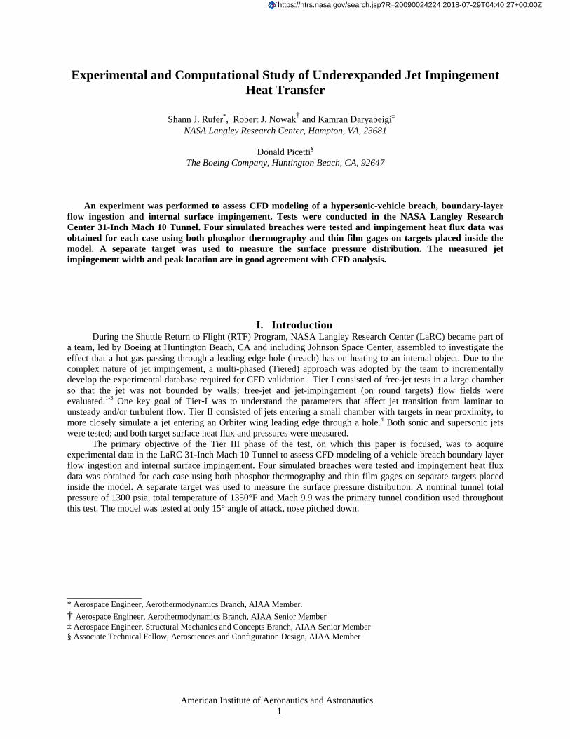
The Tier-III model design consists of two main components: (1) the actual model that is injected into the tunnel flow and (2) the gas exit system from the model through to the three-tank system which is used to control the External Jet Pressure Ratio, defined as the ratio of the flat plate external surface pressure to the internal static pressure at the exit plane of the hole, and to calculate the mass flow through the hole. The overall model is shown in Figure 1. Key components of the model are: flat plate upper surface (10 inches wide by 13.81 inches long); exhaust gas manifold/elbow assembly; exhaust gas tube and gas splitter-manifold assembly; internal targets (not seen in figure); and a strut for attaching model to tunnel injection hardware. An angle of attack of 15°, a leading edge radius of 1/16 inch, and a hole location 7.0 inches from the leading edge were selected to avoid tunnel blockage and achieve the target edge Mach number and boundary layer thickness at the breach.
CFD outflow boundary conditions – 4 static pressure ports
Figure 1 - Tier-III model configuration
American Institute of Aeronautics and Astronautics 2
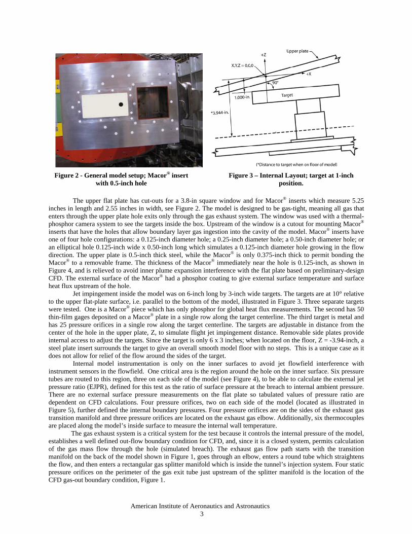
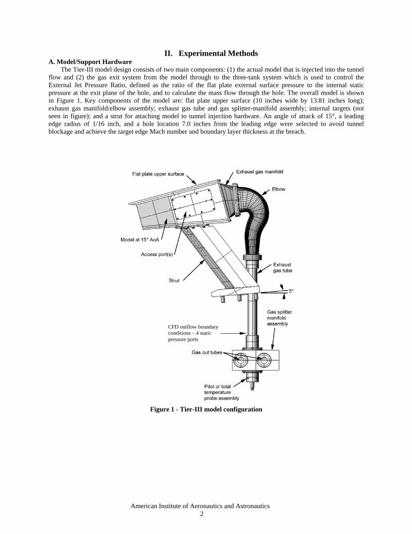
Figure 2 - General model setup; Macor® insert
with 0.5-inch hole Figure 3 – Internal Layout; target at 1-inch
position. The upper flat plate has cut-outs for a 3.8-in square window and for Macor® inserts which measure 5.25 inches in length and 2.55 inches in width, see Figure 2. The model is designed to be gas-tight, meaning all gas that enters through the upper plate hole exits only through the gas exhaust system. The window was used with a thermal-phosphor camera system to see the targets inside the box. Upstream of the window is a cutout for mounting Macor® inserts that have the holes that allow boundary layer gas ingestion into the cavity of the model. Macor® inserts have one of four hole configurations: a 0.125-inch diameter hole; a 0.25-inch diameter hole; a 0.50-inch diameter hole; or an elliptical hole 0.125-inch wide x 0.50-inch long which simulates a 0.125-inch diameter hole growing in the flow direction. The upper plate is 0.5-inch thick steel, while the Macor® is only 0.375-inch thick to permit bonding the Macor® to a removable frame. The thickness of the Macor® immediately near the hole is 0.125-inch, as shown in Figure 4, and is relieved to avoid inner plume expansion interference with the flat plate based on preliminary-design CFD. The external surface of the Macor® had a phosphor coating to give external surface temperature and surface heat flux upstream of the hole. Jet impingement inside the model was on 6-inch long by 3-inch wide targets. The targets are at 10° relative to the upper flat-plate surface, i.e. parallel to the bottom of the model, illustrated in Figure 3. Three separate targets were tested. One is a Macor® piece which has only phosphor for global heat flux measurements. The second has 50 thin-film gages deposited on a Macor® plate in a single row along the target centerline. The third target is metal and has 25 pressure orifices in a single row along the target centerline. The targets are adjustable in distance from the center of the hole in the upper plate, Z, to simulate flight jet impingement distance. Removable side plates provide internal access to adjust the targets. Since the target is only 6 x 3 inches; when located on the floor, Z = -3.94-inch, a steel plate insert surrounds the target to give an overall smooth model floor with no steps. This is a unique case as it does not allow for relief of the flow around the sides of the target. Internal model instrumentation is only on the inner surfaces to avoid jet flowfield interference with instrument sensors in the flowfield. One critical area is the region around the hole on the inner surface. Six pressure tubes are routed to this region, three on each side of the model (see Figure 4), to be able to calculate the external jet pressure ratio (EJPR), defined for this test as the ratio of surface pressure at the breach to internal ambient pressure. There are no external surface pressure measurements on the flat plate so tabulated values of pressure ratio are dependent on CFD calculations. Four pressure orifices, two on each side of the model (located as illustrated in Figure 5), further defined the internal boundary pressures. Four pressure orifices are on the sides of the exhaust gas transition manifold and three pressure orifices are located on the exhaust gas elbow. Additionally, six thermocouples are placed along the model’s inside surface to measure the internal wall temperature. The gas exhaust system is a critical system for the test because it controls the internal pressure of the model, establishes a well defined out-flow boundary condition for CFD, and, since it is a closed system, permits calculation of the gas mass flow through the hole (simulated breach). The exhaust gas flow path starts with the transition manifold on the back of the model shown in Figure 1, goes through an elbow, enters a round tube which straightens the flow, and then enters a rectangular gas splitter manifold which is inside the tunnel’s injection system. Four static pressure orifices on the perimeter of the gas exit tube just upstream of the splitter manifold is the location of the CFD gas-out boundary condition, Figure 1.
American Institute of Aeronautics and Astronautics 3
PhFPhC
PhB
Aft
PbF
PbB
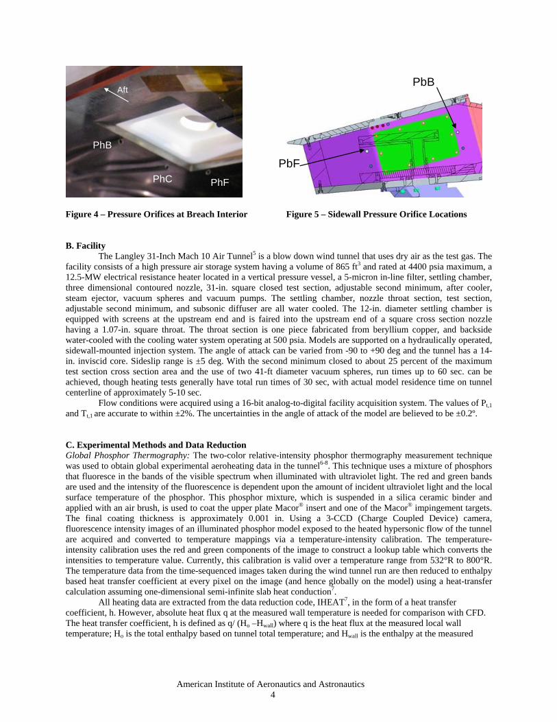
Figure 4 – Pressure Orifices at Breach Interior Figure 5 – Sidewall Pressure Orifice Locations B. Facility
The Langley 31-Inch Mach 10 Air Tunnel5 is a blow down wind tunnel that uses dry air as the test gas. The facility consists of a high pressure air storage system having a volume of 865 ft3 and rated at 4400 psia maximum, a 12.5-MW electrical resistance heater located in a vertical pressure vessel, a 5-micron in-line filter, settling chamber, three dimensional contoured nozzle, 31-in. square closed test section, adjustable second minimum, after cooler, steam ejector, vacuum spheres and vacuum pumps. The settling chamber, nozzle throat section, test section, adjustable second minimum, and subsonic diffuser are all water cooled. The 12-in. diameter settling chamber is equipped with screens at the upstream end and is faired into the upstream end of a square cross section nozzle having a 1.07-in. square throat. The throat section is one piece fabricated from beryllium copper, and backside water-cooled with the cooling water system operating at 500 psia. Models are supported on a hydraulically operated, sidewall-mounted injection system. The angle of attack can be varied from -90 to +90 deg and the tunnel has a 14-in. inviscid core. Sideslip range is ±5 deg. With the second minimum closed to about 25 percent of the maximum test section cross section area and the use of two 41-ft diameter vacuum spheres, run times up to 60 sec. can be achieved, though heating tests generally have total run times of 30 sec, with actual model residence time on tunnel centerline of approximately 5-10 sec.
Flow conditions were acquired using a 16-bit analog-to-digital facility acquisition system. The values of Pt,1 and Tt,1 are accurate to within ±2%. The uncertainties in the angle of attack of the model are believed to be ±0.2º. C. Experimental Methods and Data Reduction Global Phosphor Thermography: The two-color relative-intensity phosphor thermography measurement technique was used to obtain global experimental aeroheating data in the tunnel6-8. This technique uses a mixture of phosphors that fluoresce in the bands of the visible spectrum when illuminated with ultraviolet light. The red and green bands are used and the intensity of the fluorescence is dependent upon the amount of incident ultraviolet light and the local surface temperature of the phosphor. This phosphor mixture, which is suspended in a silica ceramic binder and applied with an air brush, is used to coat the upper plate Macor® insert and one of the Macor® impingement targets. The final coating thickness is approximately 0.001 in. Using a 3-CCD (Charge Coupled Device) camera, fluorescence intensity images of an illuminated phosphor model exposed to the heated hypersonic flow of the tunnel are acquired and converted to temperature mappings via a temperature-intensity calibration. The temperature-intensity calibration uses the red and green components of the image to construct a lookup table which converts the intensities to temperature value. Currently, this calibration is valid over a temperature range from 532°R to 800°R. The temperature data from the time-sequenced images taken during the wind tunnel run are then reduced to enthalpy based heat transfer coefficient at every pixel on the image (and hence globally on the model) using a heat-transfer calculation assuming one-dimensional semi-infinite slab heat conduction7. All heating data are extracted from the data reduction code, IHEAT7, in the form of a heat transfer coefficient, h. However, absolute heat flux q at the measured wall temperature is needed for comparison with CFD. The heat transfer coefficient, h is defined as q/ (Ho –Hwall) where q is the heat flux at the measured local wall temperature; Ho is the total enthalpy based on tunnel total temperature; and Hwall is the enthalpy at the measured
American Institute of Aeronautics and Astronautics 4
local surface temperature calculated in IHEAT, assuming a constant cp for air of 0.24 Btu/(lbm-oR). Thus the desired q at Twall is obtained as follows:
q [at Twall ] = h (Ho – Hwall at Twall). Thin Film Gages: The thin-film resistance thermometer technique is generally used to obtain benchmark heating studies within the Langley Aerothermodynamics Laboratory. In a common thin film gage, the sensor is typically a platinum or palladium film, and the substrate is a thermally insulating material such as Macor®. Typically the sensor is designed so that the thickness of the sensing element is much less than that of the substrate. Therefore, the sensing element should have a negligible effect on the heat transfer to the substrate, and the temperature measured by the sensing element can be considered identical to the temperature at the surface of the substrate. It is also assumed that there is no lateral conduction through the substrate and that heat is conducted only in the direction normal to the surface. Using these assumptions, the heating rates were calculated by using the one-dimensional, finite-volume, solid model9. The method used to reduce the thin film data is described in Hollis’ user manual for his code 1DHEAT9. For this test the front face boundary condition was the temperature versus time data recorded by the thin films and the back face was set to a fixed flux condition of q = 0. The initial condition was set to be the temperature of the gage at time = 0. All data was averaged from 4.25-4.75 seconds after trigger of the data system. Heat flux data, q, calculated from the thin-film temperature measurements are given at the measured wall temperature, Twall, at the specific time. Pressure System: Pressures are routinely measured with electronically scanned pressure (ESP) piezoresistive (silicon) sensors. ESP modules are available with different pressure ranges and typically contain 16, 32, 48, or 64 scanners. These modules may be located within or in close proximity to the model. Pressure Systems, Inc. (PSI) model 8400 measurement systems have the capability of 512 channels of pressure measurements. High volume, multi-range, variable capacitance, diaphragm-type transducers are available for certain applications. These diaphragm-type transducers were used for measurements of the very-low vacuum tank system pressures. Pressure data are averaged between 4 and 5 seconds from the start (time = 0.0) of the data-system which is initiated by the start of model injection sequence. D. Data Presentation, Quality and Uncertainty
Uncertainties in the phosphor thermography are based on surface temperature rise, and those presented here are based on historical testing with a variety of model types. On surfaces with significant temperature rise, such as windside surfaces (>70ºF), uncertainties are in the range of ±10%. For moderate temperature rise (20-30ºF), the uncertainties are roughly ±25%. More information on uncertainties in the phosphor thermography can be found in Refs. 3 and 4. The peak temperature rise on the target for this test ranged from 10ºF to as much as 125ºF depending on the size of the hole and the distance of the target from the hole. The uncertainty in the ESP pressure data is 0.1% of full scale. Several sources of uncertainties/errors in thin-film gages are discussed in Refs. 10-12. No conclusions were drawn on the build-up of these uncertainties, though are generally quoted to be on the order of ±10%.
III. Results
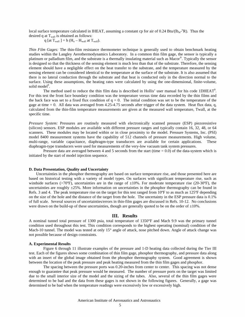
A nominal tunnel total pressure of 1300 psia, total temperature of 1350°F and Mach 9.9 was the primary tunnel condition used throughout this test. This condition corresponds to the highest operating (nominal) condition of the Mach-10 tunnel. The model was tested at only 15° angle of attack, nose pitched down. Angle of attack change was not possible because of design constraints. A. Experimental Results Figure 6 through 11 illustrate examples of the pressure and 1-D heating data collected during the Tier III test. Each of the figures shows some combination of thin film gage, phosphor thermography, and pressure data along with an insert of the global image obtained from the phosphor thermography system. Good agreement is shown between the location of the peak pressure and peak heating measured from the thin film gages and phosphor. The spacing between the pressure ports was 0.20-inches from center to center. This spacing was not dense enough to guarantee that peak pressure would be measured. The number of pressure ports on the target was limited due to the small interior size of the model and the sizing of the tubes. Also, several of the thin film gages were determined to be bad and the data from these gages is not shown in the following figures. Generally, a gage was determined to be bad when the temperature readings were excessively low or excessively high.
American Institute of Aeronautics and Astronautics 5
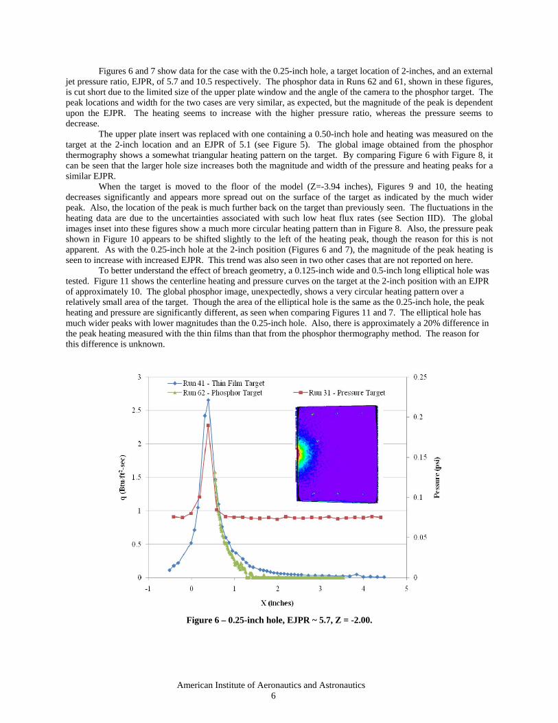
Figures 6 and 7 show data for the case with the 0.25-inch hole, a target location of 2-inches, and an external jet pressure ratio, EJPR, of 5.7 and 10.5 respectively. The phosphor data in Runs 62 and 61, shown in these figures, is cut short due to the limited size of the upper plate window and the angle of the camera to the phosphor target. The peak locations and width for the two cases are very similar, as expected, but the magnitude of the peak is dependent upon the EJPR. The heating seems to increase with the higher pressure ratio, whereas the pressure seems to decrease.
The upper plate insert was replaced with one containing a 0.50-inch hole and heating was measured on the target at the 2-inch location and an EJPR of 5.1 (see Figure 5). The global image obtained from the phosphor thermography shows a somewhat triangular heating pattern on the target. By comparing Figure 6 with Figure 8, it can be seen that the larger hole size increases both the magnitude and width of the pressure and heating peaks for a similar EJPR.
When the target is moved to the floor of the model (Z=-3.94 inches), Figures 9 and 10, the heating decreases significantly and appears more spread out on the surface of the target as indicated by the much wider peak. Also, the location of the peak is much further back on the target than previously seen. The fluctuations in the heating data are due to the uncertainties associated with such low heat flux rates (see Section IID). The global images inset into these figures show a much more circular heating pattern than in Figure 8. Also, the pressure peak shown in Figure 10 appears to be shifted slightly to the left of the heating peak, though the reason for this is not apparent. As with the 0.25-inch hole at the 2-inch position (Figures 6 and 7), the magnitude of the peak heating is seen to increase with increased EJPR. This trend was also seen in two other cases that are not reported on here. To better understand the effect of breach geometry, a 0.125-inch wide and 0.5-inch long elliptical hole was tested. Figure 11 shows the centerline heating and pressure curves on the target at the 2-inch position with an EJPR of approximately 10. The global phosphor image, unexpectedly, shows a very circular heating pattern over a relatively small area of the target. Though the area of the elliptical hole is the same as the 0.25-inch hole, the peak heating and pressure are significantly different, as seen when comparing Figures 11 and 7. The elliptical hole has much wider peaks with lower magnitudes than the 0.25-inch hole. Also, there is approximately a 20% difference in the peak heating measured with the thin films than that from the phosphor thermography method. The reason for this difference is unknown.
Figure 6 – 0.25-inch hole, EJPR ~ 5.7, Z = -2.00.
American Institute of Aeronautics and Astronautics 6
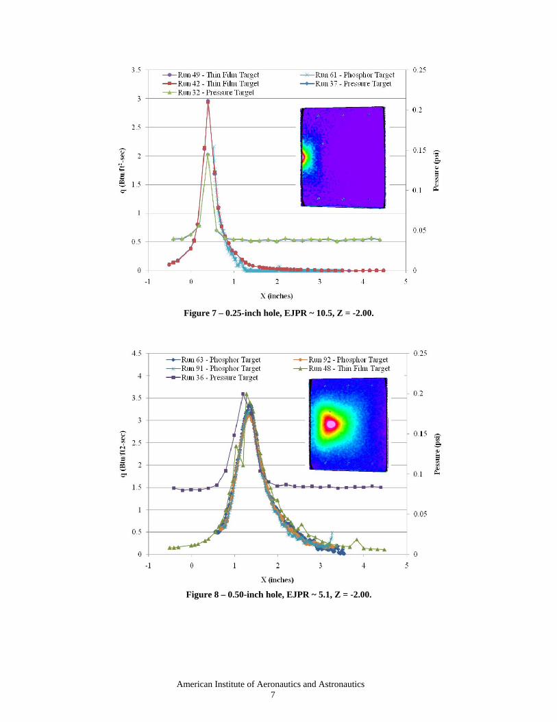
Figure 7 – 0.25-inch hole, EJPR ~ 10.5, Z = -2.00.
Figure 8 – 0.50-inch hole, EJPR ~ 5.1, Z = -2.00.
American Institute of Aeronautics and Astronautics 7
Figure 9 – 0.5-inch hole, EJPR ~ 5.0, Z= -3.94.
Figure 10 – 0.5-inch hole, EJPR ~ 8.3, Z = -3.94.
American Institute of Aeronautics and Astronautics 8
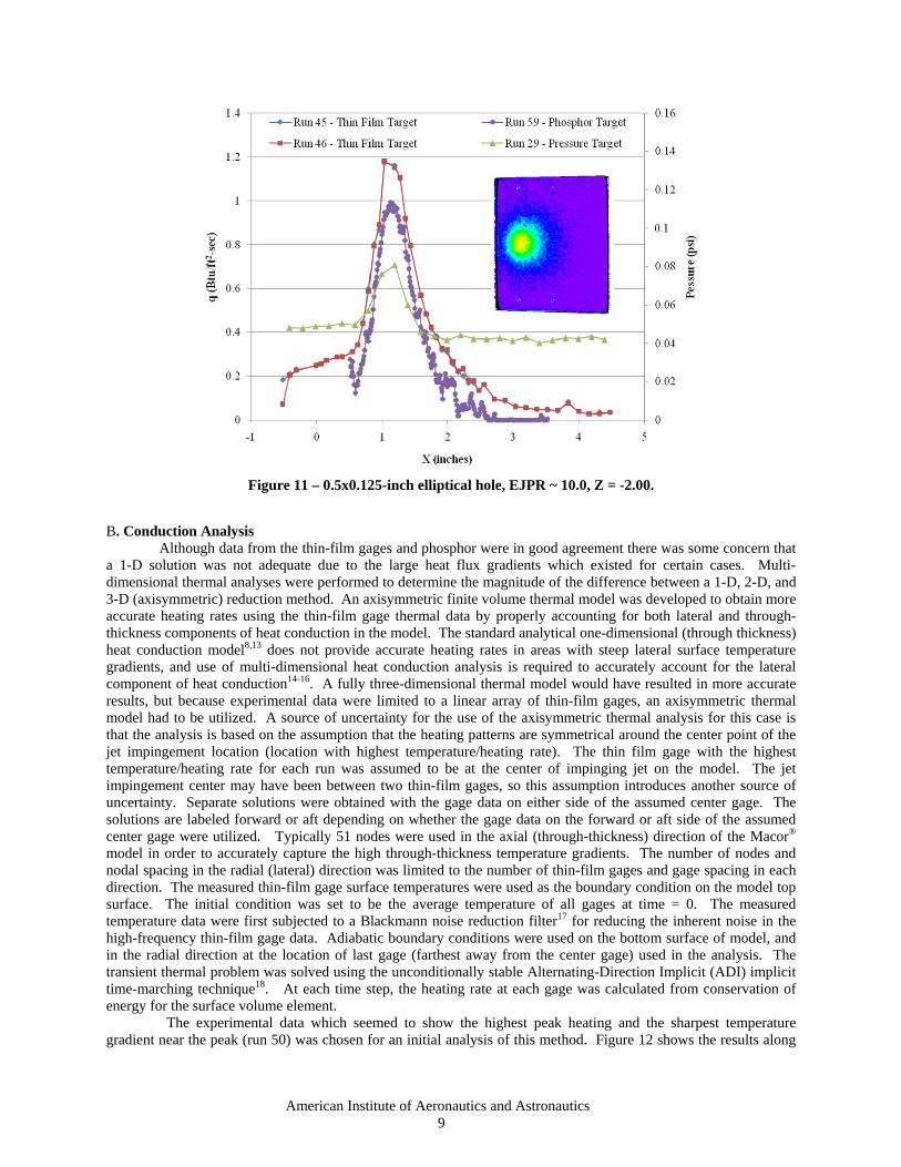
Figure 11 – 0.5x0.125-inch elliptical hole, EJPR ~ 10.0, Z = -2.00.
B. Conduction Analysis
Although data from the thin-film gages and phosphor were in good agreement there was some concern that a 1-D solution was not adequate due to the large heat flux gradients which existed for certain cases. Multi-dimensional thermal analyses were performed to determine the magnitude of the difference between a 1-D, 2-D, and 3-D (axisymmetric) reduction method. An axisymmetric finite volume thermal model was developed to obtain more accurate heating rates using the thin-film gage thermal data by properly accounting for both lateral and through-thickness components of heat conduction in the model. The standard analytical one-dimensional (through thickness) heat conduction model8,13 does not provide accurate heating rates in areas with steep lateral surface temperature gradients, and use of multi-dimensional heat conduction analysis is required to accurately account for the lateral component of heat conduction14-16. A fully three-dimensional thermal model would have resulted in more accurate results, but because experimental data were limited to a linear array of thin-film gages, an axisymmetric thermal model had to be utilized. A source of uncertainty for the use of the axisymmetric thermal analysis for this case is that the analysis is based on the assumption that the heating patterns are symmetrical around the center point of the jet impingement location (location with highest temperature/heating rate). The thin film gage with the highest temperature/heating rate for each run was assumed to be at the center of impinging jet on the model. The jet impingement center may have been between two thin-film gages, so this assumption introduces another source of uncertainty. Separate solutions were obtained with the gage data on either side of the assumed center gage. The solutions are labeled forward or aft depending on whether the gage data on the forward or aft side of the assumed center gage were utilized. Typically 51 nodes were used in the axial (through-thickness) direction of the Macor® model in order to accurately capture the high through-thickness temperature gradients. The number of nodes and nodal spacing in the radial (lateral) direction was limited to the number of thin-film gages and gage spacing in each direction. The measured thin-film gage surface temperatures were used as the boundary condition on the model top surface. The initial condition was set to be the average temperature of all gages at time = 0. The measured temperature data were first subjected to a Blackmann noise reduction filter17 for reducing the inherent noise in the high-frequency thin-film gage data. Adiabatic boundary conditions were used on the bottom surface of model, and in the radial direction at the location of last gage (farthest away from the center gage) used in the analysis. The transient thermal problem was solved using the unconditionally stable Alternating-Direction Implicit (ADI) implicit time-marching technique18. At each time step, the heating rate at each gage was calculated from conservation of energy for the surface volume element.
The experimental data which seemed to show the highest peak heating and the sharpest temperature gradient near the peak (run 50) was chosen for an initial analysis of this method. Figure 12 shows the results along
American Institute of Aeronautics and Astronautics 9
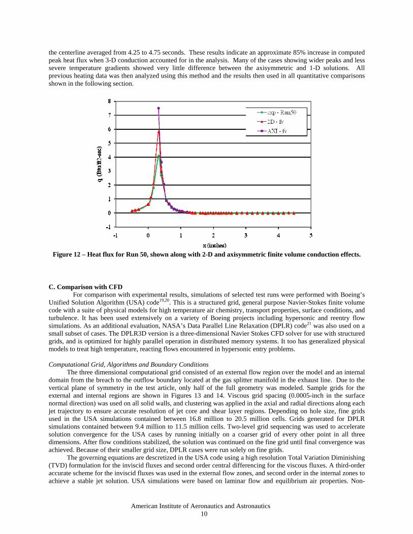
the centerline averaged from 4.25 to 4.75 seconds. These results indicate an approximate 85% increase in computed peak heat flux when 3-D conduction accounted for in the analysis. Many of the cases showing wider peaks and less severe temperature gradients showed very little difference between the axisymmetric and 1-D solutions. All previous heating data was then analyzed using this method and the results then used in all quantitative comparisons shown in the following section.
Figure 12 – Heat flux for Run 50, shown along with 2-D and axisymmetric finite volume conduction effects.
C. Comparison with CFD
For comparison with experimental results, simulations of selected test runs were performed with Boeing’s Unified Solution Algorithm (USA) code19,20. This is a structured grid, general purpose Navier-Stokes finite volume code with a suite of physical models for high temperature air chemistry, transport properties, surface conditions, and turbulence. It has been used extensively on a variety of Boeing projects including hypersonic and reentry flow simulations. As an additional evaluation, NASA’s Data Parallel Line Relaxation (DPLR) code21 was also used on a small subset of cases. The DPLR3D version is a three-dimensional Navier Stokes CFD solver for use with structured grids, and is optimized for highly parallel operation in distributed memory systems. It too has generalized physical models to treat high temperature, reacting flows encountered in hypersonic entry problems.
Computational Grid, Algorithms and Boundary Conditions
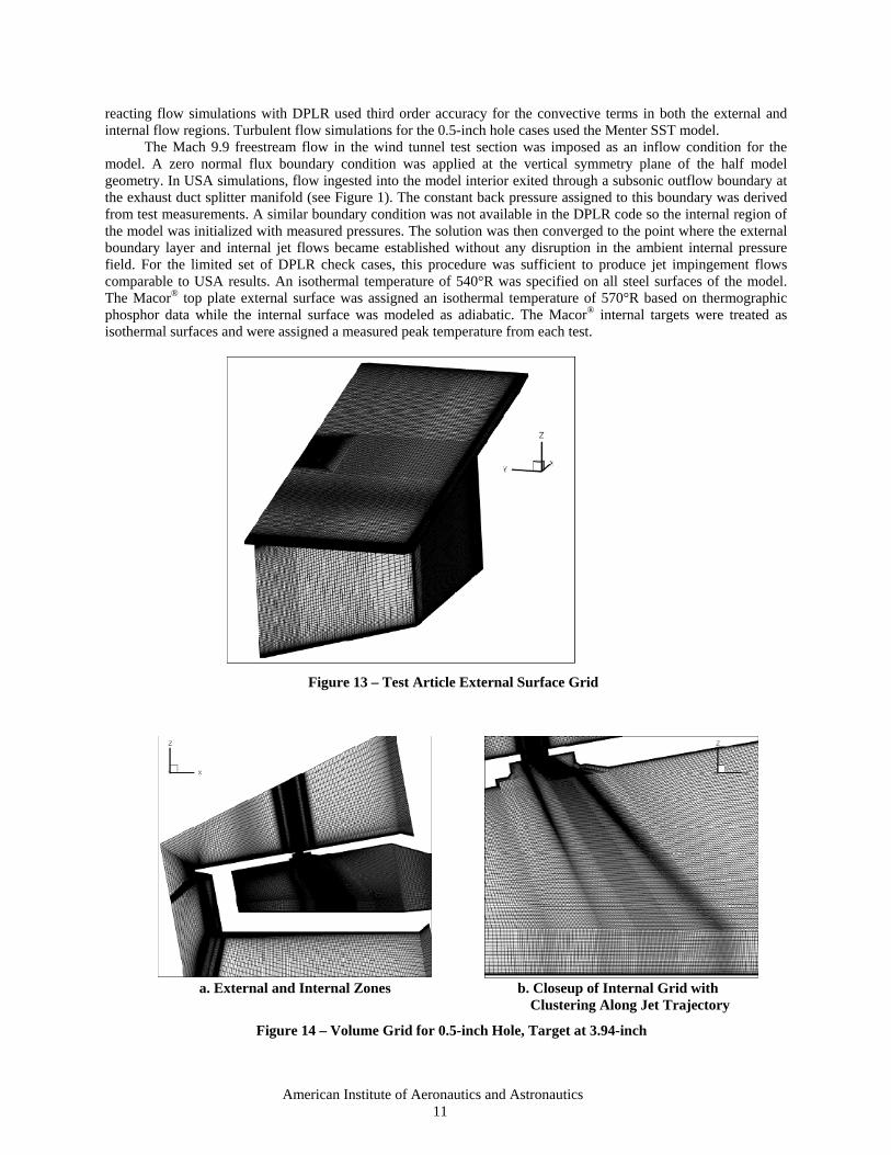
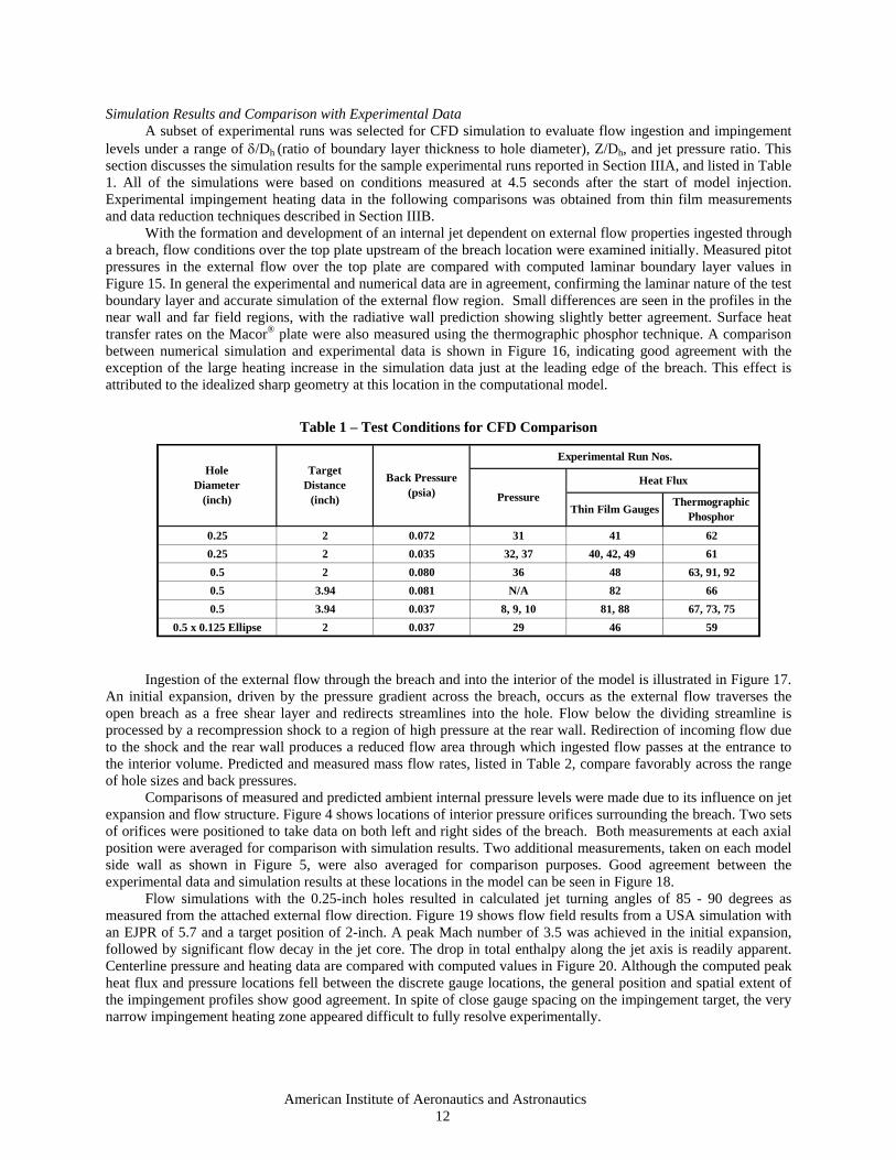
The three dimensional computational grid consisted of an external flow region over the model and an internal domain from the breach to the outflow boundary located at the gas splitter manifold in the exhaust line. Due to the vertical plane of symmetry in the test article, only half of the full geometry was modeled. Sample grids for the external and internal regions are shown in Figures 13 and 14. Viscous grid spacing (0.0005-inch in the surface normal direction) was used on all solid walls, and clustering was applied in the axial and radial directions along each jet trajectory to ensure accurate resolution of jet core and shear layer regions. Depending on hole size, fine grids used in the USA simulations contained between 16.8 million to 20.5 million cells. Grids generated for DPLR simulations contained between 9.4 million to 11.5 million cells. Two-level grid sequencing was used to accelerate solution convergence for the USA cases by running initially on a coarser grid of every other point in all three dimensions. After flow conditions stabilized, the solution was continued on the fine grid until final convergence was achieved. Because of their smaller grid size, DPLR cases were run solely on fine grids.
The governing equations are descretized in the USA code using a high resolution Total Variation Diminishing (TVD) formulation for the inviscid fluxes and second order central differencing for the viscous fluxes. A third-order accurate scheme for the inviscid fluxes was used in the external flow zones, and second order in the internal zones to achieve a stable jet solution. USA simulations were based on laminar flow and equilibrium air properties. Non-
American Institute of Aeronautics and Astronautics 10
reacting flow simulations with DPLR used third order accuracy for the convective terms in both the external and internal flow regions. Turbulent flow simulations for the 0.5-inch hole cases used the Menter SST model.
The Mach 9.9 freestream flow in the wind tunnel test section was imposed as an inflow condition for the model. A zero normal flux boundary condition was applied at the vertical symmetry plane of the half model geometry. In USA simulations, flow ingested into the model interior exited through a subsonic outflow boundary at the exhaust duct splitter manifold (see Figure 1). The constant back pressure assigned to this boundary was derived from test measurements. A similar boundary condition was not available in the DPLR code so the internal region of the model was initialized with measured pressures. The solution was then converged to the point where the external boundary layer and internal jet flows became established without any disruption in the ambient internal pressure field. For the limited set of DPLR check cases, this procedure was sufficient to produce jet impingement flows comparable to USA results. An isothermal temperature of 540°R was specified on all steel surfaces of the model. The Macor® top plate external surface was assigned an isothermal temperature of 570°R based on thermographic phosphor data while the internal surface was modeled as adiabatic. The Macor® internal targets were treated as isothermal surfaces and were assigned a measured peak temperature from each test.
Figure 13 – Test Article External Surface Grid
a. External and Internal Zones b. Closeup of Internal Grid with
Clustering Along Jet Trajectory
Figure 14 – Volume Grid for 0.5-inch Hole, Target at 3.94-inch
American Institute of Aeronautics and Astronautics 11
Simulation Results and Comparison with Experimental Data A subset of experimental runs was selected for CFD simulation to evaluate flow ingestion and impingement
levels under a range of δ/Dh (ratio of boundary layer thickness to hole diameter), Z/Dh, and jet pressure ratio. This section discusses the simulation results for the sample experimental runs reported in Section IIIA, and listed in Table 1. All of the simulations were based on conditions measured at 4.5 seconds after the start of model injection. Experimental impingement heating data in the following comparisons was obtained from thin film measurements and data reduction techniques described in Section IIIB.
With the formation and development of an internal jet dependent on external flow properties ingested through a breach, flow conditions over the top plate upstream of the breach location were examined initially. Measured pitot pressures in the external flow over the top plate are compared with computed laminar boundary layer values in Figure 15. In general the experimental and numerical data are in agreement, confirming the laminar nature of the test boundary layer and accurate simulation of the external flow region. Small differences are seen in the profiles in the near wall and far field regions, with the radiative wall prediction showing slightly better agreement. Surface heat transfer rates on the Macor® plate were also measured using the thermographic phosphor technique. A comparison between numerical simulation and experimental data is shown in Figure 16, indicating good agreement with the exception of the large heating increase in the simulation data just at the leading edge of the breach. This effect is attributed to the idealized sharp geometry at this location in the computational model.
Table 1 – Test Conditions for CFD Comparison
0.25 2 0.072 31 41 620.25 2 0.035 32, 37 40, 42, 49 610.5 2 0.080 36 48 63, 91, 920.5 3.94 0.081 N/A 82 660.5 3.94 0.037 8, 9, 10 81, 88 67, 73, 75
0.5 x 0.125 Ellipse 2 0.037 29 46 59
Back Pressure(psia)
Target Distance
(inch)
Hole Diameter
(inch)
Heat Flux
Experimental Run Nos.
Thin Film Gauges Thermographic Phosphor
Pressure
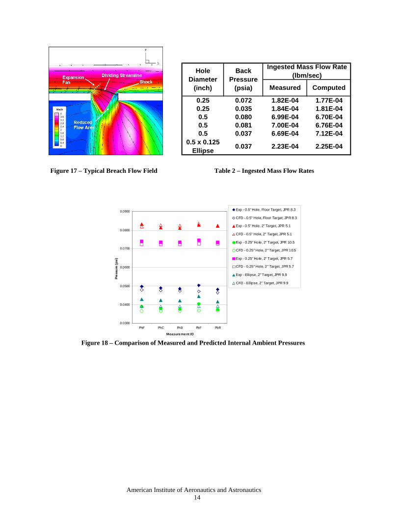
Ingestion of the external flow through the breach and into the interior of the model is illustrated in Figure 17.
An initial expansion, driven by the pressure gradient across the breach, occurs as the external flow traverses the open breach as a free shear layer and redirects streamlines into the hole. Flow below the dividing streamline is processed by a recompression shock to a region of high pressure at the rear wall. Redirection of incoming flow due to the shock and the rear wall produces a reduced flow area through which ingested flow passes at the entrance to the interior volume. Predicted and measured mass flow rates, listed in Table 2, compare favorably across the range of hole sizes and back pressures.
Comparisons of measured and predicted ambient internal pressure levels were made due to its influence on jet expansion and flow structure. Figure 4 shows locations of interior pressure orifices surrounding the breach. Two sets of orifices were positioned to take data on both left and right sides of the breach. Both measurements at each axial position were averaged for comparison with simulation results. Two additional measurements, taken on each model side wall as shown in Figure 5, were also averaged for comparison purposes. Good agreement between the experimental data and simulation results at these locations in the model can be seen in Figure 18.
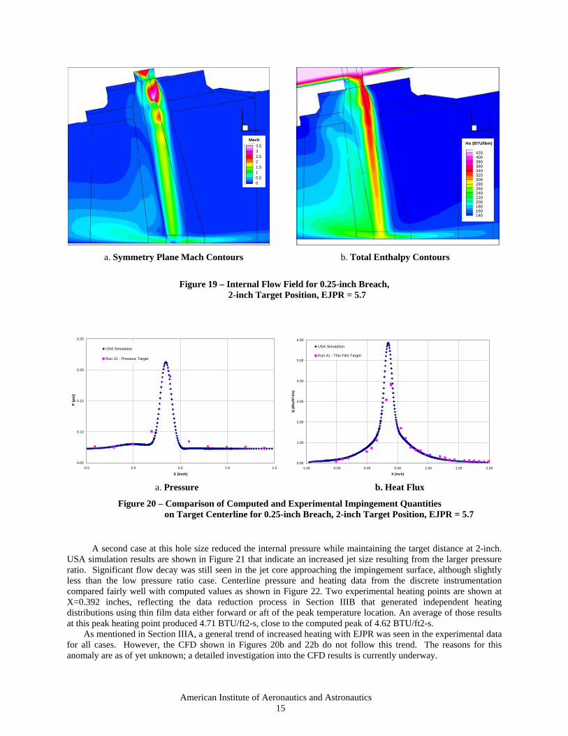
Flow simulations with the 0.25-inch holes resulted in calculated jet turning angles of 85 - 90 degrees as measured from the attached external flow direction. Figure 19 shows flow field results from a USA simulation with an EJPR of 5.7 and a target position of 2-inch. A peak Mach number of 3.5 was achieved in the initial expansion, followed by significant flow decay in the jet core. The drop in total enthalpy along the jet axis is readily apparent. Centerline pressure and heating data are compared with computed values in Figure 20. Although the computed peak heat flux and pressure locations fell between the discrete gauge locations, the general position and spatial extent of the impingement profiles show good agreement. In spite of close gauge spacing on the impingement target, the very narrow impingement heating zone appeared difficult to fully resolve experimentally.
American Institute of Aeronautics and Astronautics 12
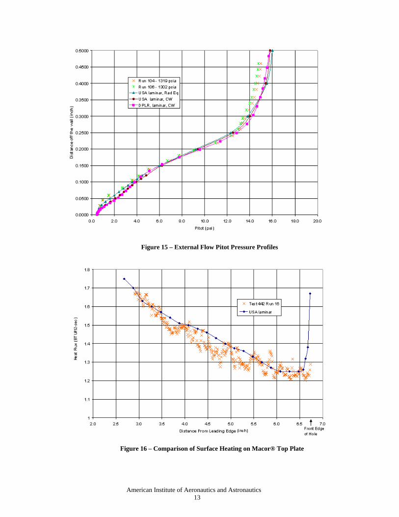
Figure 15 – External Flow Pitot Pressure Profiles
Figure 16 – Comparison of Surface Heating on Macor® Top Plate
American Institute of Aeronautics and Astronautics 13
Mach43.63.22.82.421.61.20.80.40
Mach43.63.22.82.421.61.20.80.40
0.25 0.072 1.82E-04 1.77E-040.25 0.035 1.84E-04 1.81E-040.5 0.080 6.99E-04 6.70E-040.5 0.081 7.00E-04 6.76E-040.5 0.037 6.69E-04 7.12E-04
0.5 x 0.125 Ellipse 0.037 2.23E-04 2.25E-04
Back Pressure
(psia)
Ingested Mass Flow Rate(lbm/sec)
Measured Computed
Hole Diameter
(inch)
Figure 17 – Typical Breach Flow Field Table 2 – Ingested Mass Flow Rates
0.0300
0.0400
0.0500
0.0600
0.0700
0.0800
0.0900
PhF PhC PhB PbF PbR
Measure me nt ID
Pres
sure
(ps
i)
Exp - 0.5" Hole, Floor Target, JPR 8.3
CFD - 0.5" Hole, Floor Target, JPR 8.3
Exp - 0.5" Hole, 2" Target, JPR 5.1
CFD - 0.5" Hole, 2" Target, JPR 5.1
Exp - 0.25" Hole, 2" Target, JPR 10.5
CFD - 0.25" Hole, 2" Target, JPR 10.5
Exp - 0.25" Hole, 2" Target, JPR 5.7
CFD - 0.25" Hole, 2" Target, JPR 5.7
Exp - Ellipse, 2" Target, JPR 9.9
CFD - Ellipse, 2" Target, JPR 9.9
Figure 18 – Comparison of Measured and Predicted Internal Ambient Pressures
American Institute of Aeronautics and Astronautics 14
Mach3.532.521.510.50
Mach3.532.521.510.50
420400380360340320300280260240220200180160140
Ho (BTU/lbm)
420400380360340320300280260240220200180160140
Ho (BTU/lbm)
a. Symmetry Plane Mach Contours b. Total Enthalpy Contours
Figure 19 – Internal Flow Field for 0.25-inch Breach,
2-inch Target Position, EJPR = 5.7
0.05
0.10
0.15
0.20
0.25
-0.5 0.0 0.5 1.0 1.5
X (inch)
P (p
si)
USA Simulation
Run 31 - Pressure Target
0.00
1.00
2.00
3.00
4.00
5.00
6.00
-1.00 -0.50 0.00 0.50 1.00 1.50 2.00
X (inch)
Q (B
tu/ft
^2/s
)
USA Simulation
Run 41 - Thin Film Target
a. Pressure b. Heat Flux
Figure 20 – Comparison of Computed and Experimental Impingement Quantities on Target Centerline for 0.25-inch Breach, 2-inch Target Position, EJPR = 5.7
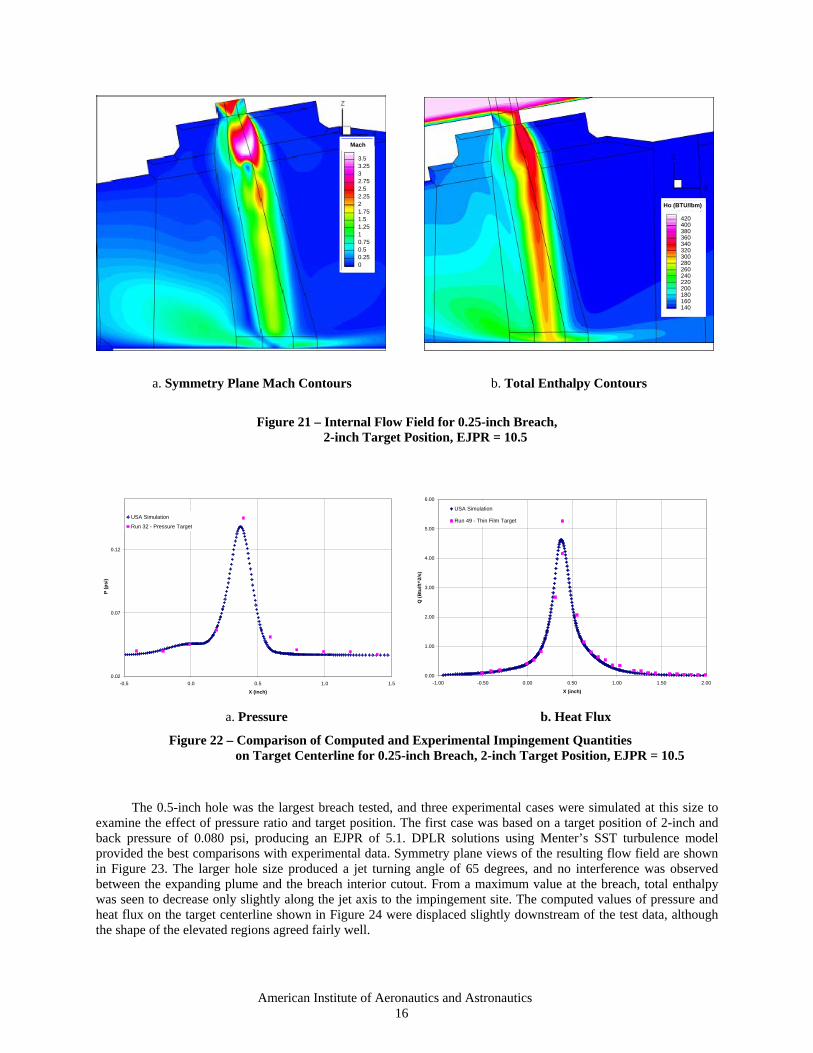
A second case at this hole size reduced the internal pressure while maintaining the target distance at 2-inch. USA simulation results are shown in Figure 21 that indicate an increased jet size resulting from the larger pressure ratio. Significant flow decay was still seen in the jet core approaching the impingement surface, although slightly less than the low pressure ratio case. Centerline pressure and heating data from the discrete instrumentation compared fairly well with computed values as shown in Figure 22. Two experimental heating points are shown at X=0.392 inches, reflecting the data reduction process in Section IIIB that generated independent heating distributions using thin film data either forward or aft of the peak temperature location. An average of those results at this peak heating point produced 4.71 BTU/ft2-s, close to the computed peak of 4.62 BTU/ft2-s.
As mentioned in Section IIIA, a general trend of increased heating with EJPR was seen in the experimental data for all cases. However, the CFD shown in Figures 20b and 22b do not follow this trend. The reasons for this anomaly are as of yet unknown; a detailed investigation into the CFD results is currently underway.
American Institute of Aeronautics and Astronautics 15
Mach
3.53.2532.752.52.2521.751.51.2510.750.50.250
Mach
3.53.2532.752.52.2521.751.51.2510.750.50.250
420400380360340320300280260240220200180160140
Ho (BTU/lbm)
420400380360340320300280260240220200180160140
Ho (BTU/lbm)
a. Symmetry Plane Mach Contours b. Total Enthalpy Contours
Figure 21 – Internal Flow Field for 0.25-inch Breach,
2-inch Target Position, EJPR = 10.5
0.02
0.07
0.12
-0.5 0.0 0.5 1.0 1.5
X (inch)
P (p
si)
USA Simulation
Run 32 - Pressure Target
0.00
1.00
2.00
3.00
4.00
5.00
6.00
-1.00 -0.50 0.00 0.50 1.00 1.50 2.00
X (inch)
Q (B
tu/ft
^2/s
)
USA Simulation
Run 49 - Thin Film Target
a. Pressure b. Heat Flux
Figure 22 – Comparison of Computed and Experimental Impingement Quantities on Target Centerline for 0.25-inch Breach, 2-inch Target Position, EJPR = 10.5
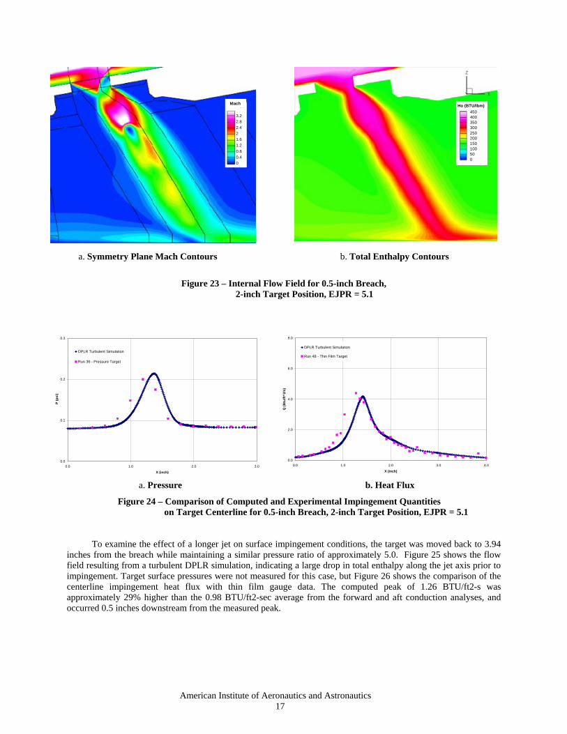
The 0.5-inch hole was the largest breach tested, and three experimental cases were simulated at this size to examine the effect of pressure ratio and target position. The first case was based on a target position of 2-inch and back pressure of 0.080 psi, producing an EJPR of 5.1. DPLR solutions using Menter’s SST turbulence model provided the best comparisons with experimental data. Symmetry plane views of the resulting flow field are shown in Figure 23. The larger hole size produced a jet turning angle of 65 degrees, and no interference was observed between the expanding plume and the breach interior cutout. From a maximum value at the breach, total enthalpy was seen to decrease only slightly along the jet axis to the impingement site. The computed values of pressure and heat flux on the target centerline shown in Figure 24 were displaced slightly downstream of the test data, although the shape of the elevated regions agreed fairly well.
American Institute of Aeronautics and Astronautics 16
Mach
3.22.82.421.61.20.80.40
Mach
3.22.82.421.61.20.80.40
450400350300250200150100500
Ho (BTU/lbm)450400350300250200150100500
Ho (BTU/lbm)
a. Symmetry Plane Mach Contours b. Total Enthalpy Contours
Figure 23 – Internal Flow Field for 0.5-inch Breach,
2-inch Target Position, EJPR = 5.1
0.0
0.1
0.2
0.3
0.0 1.0 2.0 3.0
X (inch)
P (p
si)
DPLR Turbulent Simulation
Run 36 - Pressure Target
0.0
2.0
4.0
6.0
8.0
0.0 1.0 2.0 3.0 4.0
X (inch)
Q (B
tu/ft
^2/s
)
DPLR Turbulent Simulation
Run 48 - Thin Film Target
a. Pressure b. Heat Flux
Figure 24 – Comparison of Computed and Experimental Impingement Quantities on Target Centerline for 0.5-inch Breach, 2-inch Target Position, EJPR = 5.1
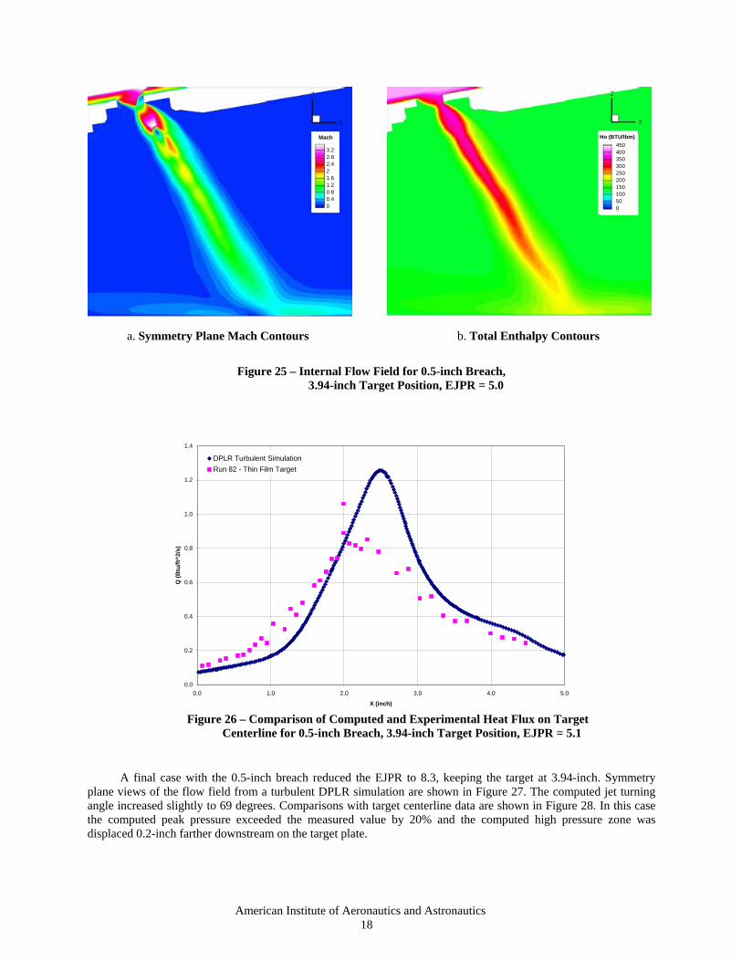
To examine the effect of a longer jet on surface impingement conditions, the target was moved back to 3.94 inches from the breach while maintaining a similar pressure ratio of approximately 5.0. Figure 25 shows the flow field resulting from a turbulent DPLR simulation, indicating a large drop in total enthalpy along the jet axis prior to impingement. Target surface pressures were not measured for this case, but Figure 26 shows the comparison of the centerline impingement heat flux with thin film gauge data. The computed peak of 1.26 BTU/ft2-s was approximately 29% higher than the 0.98 BTU/ft2-sec average from the forward and aft conduction analyses, and occurred 0.5 inches downstream from the measured peak.
American Institute of Aeronautics and Astronautics 17
Mach
3.22.82.421.61.20.80.40
Mach
3.22.82.421.61.20.80.40
450400350300250200150100500
Ho (BTU/lbm)450400350300250200150100500
Ho (BTU/lbm)
a. Symmetry Plane Mach Contours b. Total Enthalpy Contours
Figure 25 – Internal Flow Field for 0.5-inch Breach,
3.94-inch Target Position, EJPR = 5.0
0.0
0.2
0.4
0.6
0.8
1.0
1.2
1.4
0.0 1.0 2.0 3.0 4.0 5.0
X (inch)
Q (B
tu/ft
^2/s
)
DPLR Turbulent SimulationRun 82 - Thin Film Target
Figure 26 – Comparison of Computed and Experimental Heat Flux on Target
Centerline for 0.5-inch Breach, 3.94-inch Target Position, EJPR = 5.1
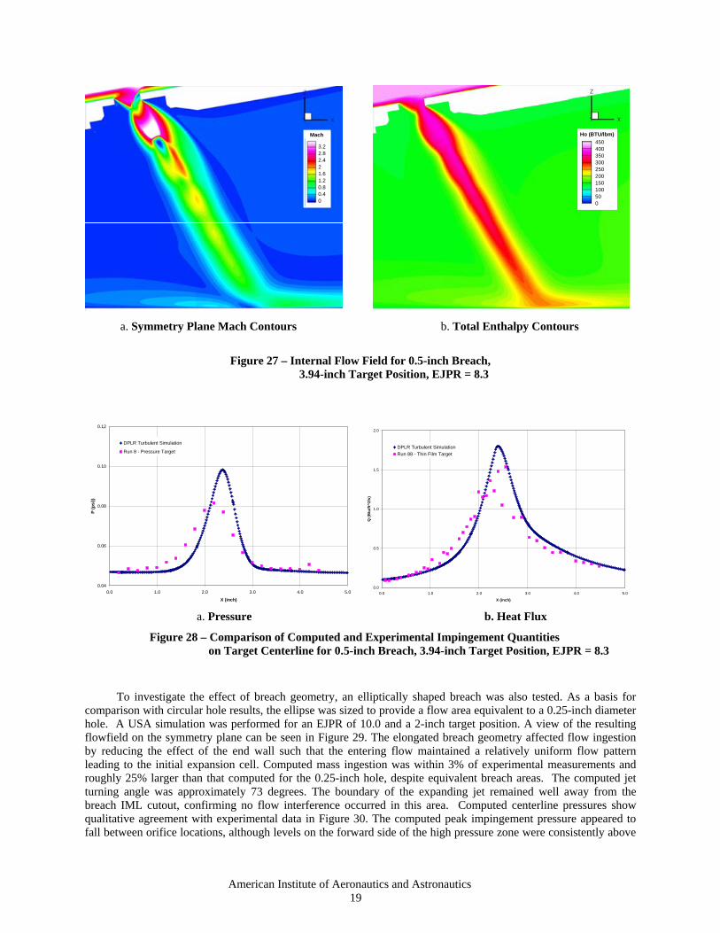
A final case with the 0.5-inch breach reduced the EJPR to 8.3, keeping the target at 3.94-inch. Symmetry plane views of the flow field from a turbulent DPLR simulation are shown in Figure 27. The computed jet turning angle increased slightly to 69 degrees. Comparisons with target centerline data are shown in Figure 28. In this case the computed peak pressure exceeded the measured value by 20% and the computed high pressure zone was displaced 0.2-inch farther downstream on the target plate.
American Institute of Aeronautics and Astronautics 18
Mach
3.22.82.421.61.20.80.40
Mach
3.22.82.421.61.20.80.40
450400350300250200150100500
Ho (BTU/lbm)450400350300250200150100500
Ho (BTU/lbm)
a. Symmetry Plane Mach Contours b. Total Enthalpy Contours
Figure 27 – Internal Flow Field for 0.5-inch Breach,
3.94-inch Target Position, EJPR = 8.3
0.04
0.06
0.08
0.10
0.12
0.0 1.0 2.0 3.0 4.0 5.0
X (inch)
P (p
si))
DPLR Turbulent Simulation
Run 8 - Pressure Target
0.0
0.5
1.0
1.5
2.0
0.0 1.0 2.0 3.0 4.0 5.0
X (inch)
Q (B
tu/ft
^2/s
)
DPLR Turbulent SimulationRun 88 - Thin Film Target
a. Pressure b. Heat Flux
Figure 28 – Comparison of Computed and Experimental Impingement Quantities on Target Centerline for 0.5-inch Breach, 3.94-inch Target Position, EJPR = 8.3
To investigate the effect of breach geometry, an elliptically shaped breach was also tested. As a basis for comparison with circular hole results, the ellipse was sized to provide a flow area equivalent to a 0.25-inch diameter hole. A USA simulation was performed for an EJPR of 10.0 and a 2-inch target position. A view of the resulting flowfield on the symmetry plane can be seen in Figure 29. The elongated breach geometry affected flow ingestion by reducing the effect of the end wall such that the entering flow maintained a relatively uniform flow pattern leading to the initial expansion cell. Computed mass ingestion was within 3% of experimental measurements and roughly 25% larger than that computed for the 0.25-inch hole, despite equivalent breach areas. The computed jet turning angle was approximately 73 degrees. The boundary of the expanding jet remained well away from the breach IML cutout, confirming no flow interference occurred in this area. Computed centerline pressures show qualitative agreement with experimental data in Figure 30. The computed peak impingement pressure appeared to fall between orifice locations, although levels on the forward side of the high pressure zone were consistently above
American Institute of Aeronautics and Astronautics 19
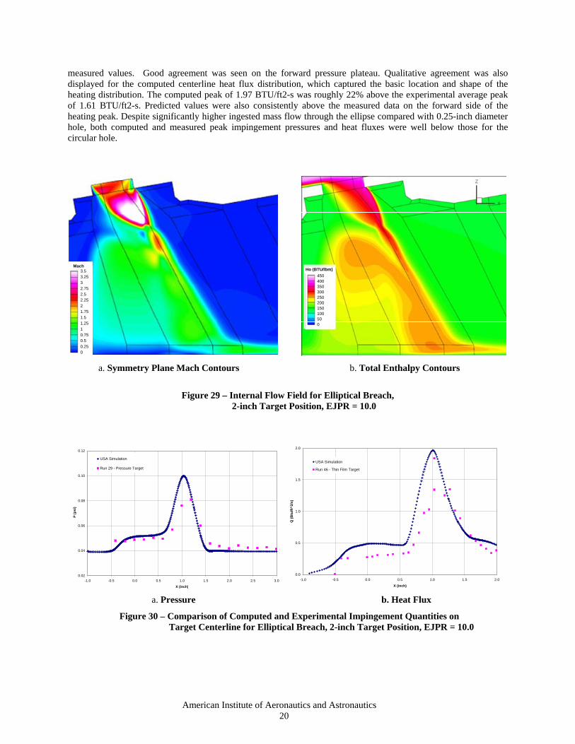
measured values. Good agreement was seen on the forward pressure plateau. Qualitative agreement was also displayed for the computed centerline heat flux distribution, which captured the basic location and shape of the heating distribution. The computed peak of 1.97 BTU/ft2-s was roughly 22% above the experimental average peak of 1.61 BTU/ft2-s. Predicted values were also consistently above the measured data on the forward side of the heating peak. Despite significantly higher ingested mass flow through the ellipse compared with 0.25-inch diameter hole, both computed and measured peak impingement pressures and heat fluxes were well below those for the circular hole.
Mach3.53.2532.752.52.2521.751.51.2510.750.50.250
Mach3.53.2532.752.52.2521.751.51.2510.750.50.250
450400350300250200150100500
Ho (BTU/lbm)450400350300250200150100500
Ho (BTU/lbm)
a. Symmetry Plane Mach Contours b. Total Enthalpy Contours
Figure 29 – Internal Flow Field for Elliptical Breach,
2-inch Target Position, EJPR = 10.0
0.02
0.04
0.06
0.08
0.10
0.12
-1.0 -0.5 0.0 0.5 1.0 1.5 2.0 2.5 3.0
X (inch)
P (p
si)
USA Simulation
Run 29 - Pressure Target
0.0
0.5
1.0
1.5
2.0
-1.0 -0.5 0.0 0.5 1.0 1.5 2.0
X (inch)
Q (B
tu/ft
^2/s
)
USA Simulation
Run 46 - Thin Film Target
a. Pressure b. Heat Flux
Figure 30 – Comparison of Computed and Experimental Impingement Quantities on Target Centerline for Elliptical Breach, 2-inch Target Position, EJPR = 10.0
American Institute of Aeronautics and Astronautics 20
IV. Concluding Remarks Experimental data was acquired in the LaRC 31-Inch Mach 10 Tunnel to assess CFD modeling of a vehicle
breach boundary layer flow ingestion and internal surface impingement. Four simulated breaches were tested and impingement data was obtained for each case using both phosphor thermography and thin-film gages on separate targets placed inside the model. A third target was used to measure the surface pressure distribution.
Jet impingement heat flux data from thin film gages and global thermographic methods appear to be in good agreement. The effects of 3-D conduction appear to have a significant effect on the calculated heat flux, especially for cases with very narrow, high magnitude peak heating. The jet impingement width and peak location are in good agreement between data from pressure, thin film gages, and thermographic phosphor data and CFD analysis. Also, comparisons between the axisymmetric conduction analysis from the measured thin film data and the CFD analysis show good agreement in the magnitude of the heating peaks in most cases.
Acknowledgments The authors would like to thank the following people for their contributions to the project: Mike Langford,
Richard Wheless, John Hopkins, Vince Cruz, Mike Powers, Mark Griffith, Tom Hall, Wayne Geouge and Pete Veneris for their assistance in model design, fabrication and preparation; Tony Robbins, Johnny Ellis, Paul Tucker, Henry Fitzgerald and Doug Boggs for wind tunnel support; Kevin Hollingsworth, Sheila Wright and Stanley Mason for data acquisition assistance; Suk Kim and Eliko Ikeda for pretest and posttest CFD analysis.. Without their help, these tests would not have been possible.
References
1 Wilkes, J. A., Danehy, P. M., and Nowak, R. J.: “Fluorescence Imaging Study of Transition in Underexpanded Free Jets,” Proceedings of the 21st International Congress on Instrumentation in Aerospace Simulation Facilities (ICIASF)[CD-ROM], Sendai, Japan, August 29 - September 1, 2005, pp. 1-8.
2 Wilkes, J.A., Glass, C. E., Danehy, P. M., and Nowak, R. J.: “Fluorescence Imaging of Underexpanded Jets and Comparison with CFD,” 44th AIAA Aerospace Sciences Meeting and Exhibit, Reno, NV, January 9-12, 2006. AIAA 2006-910
3 Inman, Jennifer Ann: "Fluorescence Imaging Study of Free and Impinging Supersonic Jets: Jet Structure and Turbulent Transition." Ph.D. Dissertation, College of William and Mary, Virginia, 2007.
4 Nowak, Robert J., Picetti, Donald J., and Liechty, Derek S., "Tier-II Breaches Jet Impingement Tests, NASA LaRC 31-Inch Mach-10 Tunnel," NASA EG-SS-06-6, November 01, 2006.
5 Micol, J. R., "Langley aerothermodynamics facilities complex: enhancements and testing capabilities," AIAA-98-0147, Jan 1998.
6 Buck, G. M., “Automated thermal mapping techniques using chromatic image analysis," NASA TM-101554, April 1989.
7 Merski, N. R., "Reduction and analysis of phosphor thermography data with iheat software package," AIAA-98-0712, Jan 1998.
8 Merski, N. R., "Global aeroheating wind-tunnel measurements using improved two-color phosphor thermography model," Journal of Spacecraft and Rockets, Vol., 36, No., 2, 1998, pp. 160-170.
9 Hollis, Brian R.: “User’s Manual for the One-Dimensional Hypersonic Experimental Aero-Thermodynamic (1DHEAT) Data Reduction Code,” NASA Contractor Report 4691, August 1995.
10 Miller, Charles G., III, Micol, John R., and Gnoffo, Perter A., "Laminar Heat-Transfer Distributions on Biconics at Incidence in Hypersnoic-Hypervelocity Flows," NASA TP-2213, 1984.
11 Miller, Charles G., III, "Comparison of Thin-Film Resistance Heat-Transfer Gages with Thin-Skin Transient Calorimeter Gages in Conventional-Hypersonic Wind Tunnels," NASA TM-83197, 1981.
12 Micol, J.R., "Hypersonic Aerodynamic/Aerothermodynamic Testing Capabilities at Langley Research Center: Aerothermodynamic Facilities Complex," AIAA-95-2107, June 1995.
13 Cook, W. J., and Felderman, E. J., “Reduction of Data from Thin Film Heat Transfer Gages: A Concise Numerical Technique,” AIAA Journal, Vol. 4, No. 3, 1966, pp. 561-562.
14 Daryabeigi, K., Berry, S. A., Horvath, T. J., and Nowak, R. J., “Finite Volume Numerical Methods for Aeroheating Rate Calculations From Infrared Thermographic Data,” Journal of Spacecraft and Rockets, Vol. 43, No. 1, 2006, pp. 54-62.
American Institute of Aeronautics and Astronautics 21

American Institute of Aeronautics and Astronautics 22
15 Walker, D. G., Scott, E. P., and Nowak, R. J., “Estimation Methods for Two-Dimensional Conduction Effects of Shock-Shock Heat Fluxes,” Journal of Thermophysics and Heat Transfer, Vol. 14, No. 4, 2000, pp. 533-539.
16 Coblish, J. J., Smith, M. S., Hand, T., Candler, G. V., and Nompelis, I., “Double-Cone Experiment and Numerical Analysis at AEDC Hypervelocity Wind Tunnel 9,” AIAA 2005-0902, January 2005.
17 Smith, S. A., Digital Signal Processing, A Practical Guide for Engineers and Scientists, Elsevier Science, Burlington, MA, 2003.
18 Anderson, D. A., Tannehill, J. C., and Pletcher, R. H., Computational Fluid Mechanics and Heat Transfer, Hemisphere Publishing, Washington, 1984.
19 Chakravarthy, S. R., Szema, K. Y., and Haney, J. W., "Unified Nose-to-Tail Computational Method for Hypersonic Vehicle Applications," AIAA-1988-2564, June 1988.
20 Ota, D. K., Chakravarthy, S. R., and Darling, J. C., "An Equilibrium Air Navier-Stokes Code For Hypersonic Flows," AIAA-1988-0419, June 1988.
21 Wright, M. J., Candler, G. V., and Bose, D., "Data-Parallel Line Relaxation Method for the Navier-Stokes Equations," AIAA Journal, Vol. 36, No. 9, Sept. 1998, pp 1603-1609.