Experimental and Characterization Techniques II.1...

Chapter II

Department of Materials Science 46

CHAPTER II

Experimental and Characterization Techniques

II.1 Introduction:

Carbon and ceramic foams are of great interest, because of their properties like light

weight, low density, high chemical resistance, good thermal shock resistance and potential

tailor-ability of their physical properties from insulator to conducting material. Numbers of

methods used for development of carbon and silica foam are known. In the present work,

template method has been used for development of carbon and silica foams. The chapter

includes:

1. Development of carbon foam

2. Functionalization of carbon foam

3. Development of silica foam

4. Characterization techniques

The carbon and silica foams have been characterized for their composition, physical,

thermal, microstructure and mechanical properties. The characterization techniques used for

analyses have been described in this chapter.

Prepared carbon and silica foam were also analyzed using statistical data analysis

software (SPSS and MINITAB) to estimate dimensional shrinkage observed after heat

treatment at 1000 °C. Linear equations were obtained for estimation of linear shrinkage

observed in length, breadth and height.

II.2 Development of carbon foam:

Carbon foams were developed by using template route. Commercially available open

cell polyurethane (PU) foam was used as template and phenolic resin was used as carbon

precursor. PU foams were impregnated with phenolic resin solution and cured. Carbonization

of cured foam was carried out up to 1000 °C in an inert atmosphere to make carbon foam.

Chapter II


The carbon foams were characterized for their volume shrinkage, change in density,

crystallinity, porosity, permeability, specific heat, co-efficient of thermal expansion, surface

morphology, mechanical properties, etc.

II.2.1 Materials used:

Commercially available open cell polyurethane foams

Phenolic resin, Kemrock Industries and Export Limited.

Methanol, [99.5%]

Gases: Nitrogen (99.98%), Argon (99.99%), from Vadilal Gas Industries at

Vadodara.

II.2.2 Characteristics of Polyurethane foam:

Open cell polyurethane (PU) foams, commercially available were collected having

different densities shown in figure II.1. There were of different colours.

Figure II.1: PU foam having different density

Open cell PU foams used were characterized for their density. The densities of

different foams were calculated and table II.1 gives density of different types of foam. The

density varies from 0.02 to 0.04 g/cc.

Chapter II


Table II.1: Density of different PU foams

II.2.3 Properties of phenolic resin:

Phenolic resin was used as carbon precursor for making carbon foam. The

specifications of phenolic resin used are given in table II.2:

Table II.2: Specification of phenolic resin

Appearance : Clear brownish viscous liquid

Viscosity @ 25 ⁰C : 2008 cp

Specific gravity @ 25 ⁰C : 1.23

Moisture content : 11 %

pH : 6.4

Refractive index : 1.570

Non-volatile content : 76 %

Resin/catalyst ratio : 100/7 part

II.2.4 Preparation of foams:

The open cell PU foams having density of 0.04 g/cc were selected for development of

foam. The foams were washed in distilled water and dried in oven at 100 °C. The colour of

PU foam was pink. Cleaned PU foams were cut into small rectangular and square pieces.

Dimensions of PU foam pieces were taken using vernier callipers and mass by using

electronic balance LIBROR AGE-220 (Shimadzu co. Japan).

No. Colour PU foam density, gm/cc

i White 0.020

ii Yellow 0.024

iii Dark grey 0.026

iv Orange 0.036

v Pink 0.040

Chapter II


II.2.5 Preparation of resin solution:

The resin solution was made by using methanol as a solvent. Mixture of methanol and

phenolic resin were prepared in different ratio and change in viscosity of these mixtures of

phenolic resin and methanol was measured using Brookfield viscometer. Calibration curve

was prepared for resin to methanol ratio from 10 : 90 to 100 : 0. Change in density of

mixture of phenolic resin and methanol were measured using weight to volume ratio.

II.2.6 Impregnation of phenolic resin

Cleaned PU foam was impregnated with phenolic resin. For that PU foam was dipped

into beaker filled with phenolic resin. The excess resin was removed from time to time to

achieve uniform impregnation. Figure II.2 shows physical observation of resin impregnated

cured foam from inside. Incomplete impregnation results into the voids or vacant space in

final carbon foam. The presence of extra resin in the sample may close some pores or having

dead end at the bottom.

Figure II.2: Cross-section image of incomplete (left) and complete impregnated (right) foam

By carrying out multiple impregnations, it was found that 13 ml resin solution was

sufficient for impregnation of 50 cc PU foam.

Chapter II


II.2.7 Drying and curing of foams:

Drying of resin impregnated foam was carried out in oven at 150 °C. To enhance the

degree of cross linking between phenolic chains, impregnated PU foams were cured at 150

oC overnight. The change in color of foam appeared to be dark brown as shown in figure

II.2 and II.4.

II.2.8 Carbonization:

The cured foams were carbonized at 1000 °C in nitrogen atmosphere. The

carbonization assembly used for making carbon foam is shown in figure II.3. Carbonization

was carried out in carbonization reactor having gas outlet and inlet on same side. The reactor

was made up of stainless steel material. The S.S. container was placed in a muffle furnace

which was heated electrically. Heating and cooling rate of the furnace was controlled by

temperature programmer. The temperature of furnace was measured using chromel-alumel

thermocouple and CHINO-KP1000 temperature programmer/controller was used to maintain

the temperature of furnace. High purity Nitrogen gas was used during carbonization as an

inert gas.

Figure II.3: Set up for carbonization

Chapter II


Schematic diagram for development of carbon foam is shown in figure II.4.

Figure II.4: Schematic diagram for development of carbon foam

II.2.9 Heat treatments:

Carbon foams heat treated at 1000 °C were heated at different temperature as given

below:

1) In nitrogen atmosphere at 1000 °C

2) In argon atmosphere at 1200, 1400 and 1600 °C.

High temperature heat treatment was carried out in graphite boat in alumina tubular

furnace. Figure II.5 shows furnace used for high temperature heat treatment. Heating and

cooling rate was 300 °C/ hr. Samples were soaked for 1hour at 1200, 1400 and 1600 °C

temperature.

Chapter II


Figure II.5: Agni furnace for high temperature heat treatment

II.2.10 Functionalization of carbon foam:

Carbon foams developed by using template route were chemically functionalized by

treatment with concentrated nitric acid at 100 °C. Figure II.6 shows schematic diagram for

functionalization of carbon foam. Figure II.7 shows set up used for functionalization of

carbon foam.

Weighed carbon foam samples were placed in 4 N nitric acid solution in volumetric

flask and refluxed for different time intervals, of 3, 6, 7, 8 and 9 hours. The acid treated

samples were washed thoroughly with distilled water to free them of nitrate ions till neutral

pH was achieved. These were dried in oven at 150 °C. The type and amount of surface

oxygen functionalities formed on the surface were determined using Boehm’s titration and

FTIR analysis.

Chapter II


Figure II.6: Schematic diagram for functionalization of carbon foam

Figure II.7: Set up for acid treatment of carbon foam

II.3 Development of silica foam:

Silica foam was developed by using template method. Polyurethane foams of lower

density were used as template to get highly interconnected porous network. Silica sol was

prepared using sol gel route and it was impregnated into the PU template. Sintering of sol

impregnated dried samples were carried out at 1000 °C in air, to make silica foam. Silica

Chapter II


foams were characterized for different properties e.g. crystallinity, acid/base resistance,

thermal, compressive strength.

II.3.1 Materials used:

Open cell PU foam, (density: 0.02 g/cc)

Tetraethyl orthosilicate (TEOS, Si(OC2H5)4), Sigma-Aldrich

Ethanol (C2H5OH) (99.5 %)

Hydrochloric acid [HCl],(36 %)

Distilled water [H2O]

Nitric acid, [HNO3], (70 %)

Sulphuric acid, [H2SO4], (98 %)

Sodium hydroxide, [NaOH], (98 %)

Potassium hydroxide, [KOH], (85 %)

Sodium bicarbonate, [Na2CO3], (100 %)

II.3.2 Preparation of silica sol:

Silica sol was prepared by hydrolysis of Tetraethoxysilane, Si(OC2H5)4, with acidified

water. Ethanol was used as a solvent for TEOS. 2 moles of ethanol and 1 mole of TEOS were

mixed in a flask using magnetic stirrer (shown in figure II.8). The hydrolysis of TEOS was

carried with acidified water using TEOS : H2O from 1 : 2 to 1 : 6. Acidified water was added

drop wise into solution of TEOS and ethanol. Hydrolysis reaction was carried out for 70 hrs.

Chapter II


Figure II.8: Set up used for preparation of silica sol

Kinetics of hydrolysis of silica sol was studied using UV-VIS spectrophotometer by

measuring λmax of TEOS, ethanol and water mixture at different time interval. Figure II.9

shows the UV-VIS spectrophotometer. (Shimadzu UV1601, Double Beam Optics with

Halogen Light Source, Spectral Resolution Power: 2 nm)

Figure II.9: UV-VIS spectrophotometer. (Shimadzu UV1601)

Chapter II


II.3.3 Impregnation of silica sol:

PU foams were cleaned, cut into small rectangular pieces and dried at 100 °C in oven.

PU foam having 0.02 g/cc density (white in colour) was used as template. Silica sol was

impregnated in PU foam by dipping and drying. By number of experiments it was concluded

that 40 cc volume PU foam was required for 25 ml silica sol.

II.3.4 Drying of foams:

Drying was carried out in conventional oven as well as in microwave oven. The

conventional vacuum oven used is shown in figure II.10. The drying of foam was carried out

at 100 °C. The uneven shrinkage and small deformation were seen as shown in figure II.11.

II.10: Conventional vacuum oven used for drying

Figure II.11: Drying of silica sol impregnated PU foam by Conventional method

Chapter II


To overcome these uneven shrinkage and deformation, microwave drying was carried

out. The microwave oven used is shown in figure II.12. Silica sol impregnated PU foam was

dried using microwave oven at different power levels as shown in table II.3 and up to

800 watt power level was used for drying foams. During drying, the sample was overturned

as to have uniform drying of sol in the sample.

.

Figure II.12: Microwave oven (Whirlpool, Model: JT 368)

Table II.3: Steps for microwave drying of sol impregnated PU sample

Power level I side II side III side IV side

500 watt 15 s 15 s 15 s 15 s

800 watt 15 s 15 s 15 s 15 s

Figure II.13: Drying of silica sol impregnated PU foam using Microwave oven

Chapter II


The pink and white colour PU foams were used as template shown in figure II.13.

Microwave drying of silica sol impregnated PU foams show uniform drying without warping

at edges and in the centre.

II.3.5 Heat treatment of foams:

The silica impregnated dried foams were sintered at 1000°C in furnace, shown in

figure II.4. Silica foams were further heat treated at high temperature in furnace shown in

figure II.5. Various heating rates were used during heat treatment of silica impregnated dried

foam to obtain good strength. Hold time was varied from 1 to 5 hours at 570, 650, 870 and

1000 °C. Maximum strength of silica foam was obtained using heating rate profile given in

figure II.14. Silica foams were further heat treated up to 1600°C at 300°C/hr heating and

cooling rate with 1 hour hold time.

Figure II.14: Heating rate profile used for sintering

Schematic diagram for development of silica foam is shown in figure II.15. The

prepared silica foams were characterized for different properties.

Chapter II


Figure II.15: Schematic diagram for development of silica foam

II.4 Characterization of foams:

II.4.1 Physical properties:

II.4.1.1 Volume shrinkage:

The reduction in length, breadth and thickness during carbonization and sintering was

measured by measuring dimensions both before and after heat treatment using vernier

callipers. The shrinkage in all direction was calculated by using formula:

where,

Lbefore – Length before heat treatment, mm

Lafter – Length after heat treatment, mm

Likewise, shrinkage in breadth and thickness was determined by above formula.

Chapter II


II.4.1.2 Carbon yield, (%):

Carbon yield was calculated from the initial weight of materials (W1) before

carbonization and final weight of carbon (W2) obtained after carbonization using following

relation.

II.4.1.3. Density Measurement:

Bulk density of the samples was theoretically calculated. Geometric volume of sample

was calculated by measuring length, breadth and thickness of foam with the help of vernier

calipers.

Volume of sample (V) = l b t

Where, l = length of the sample

b = breadth of the sample

t = thickness of the sample

Density of sample was determined using following formula:

II.4.1.4 Porosity:

II.4.1.4.1 Kerosene porosity:

The kerosene pick-up method was used for determination of open porosity of

developed carbon and silica foams. Figure II.16 shows set-up used for determination of

kerosene porosity of foams. It consists of a glass flask connected to a kerosene reservoir and

vacuum system with stopcocks. One stopcock was joined in between flask and kerosene

reservoir and the second stop cork was joined in between flask and vacuum system.

A small piece of foam of known measured dimensions was taken and weighed. It was

placed in the round bottom flask. Flask was connected with vacuum system by opening

Chapter II


stopcock 2. The sample was evacuated at 10-3

torr for one hour with the help of vacuum

pump to clean the sample. The stopcock -2 was closed after evacuation for one hour and

kerosene was allowed to flow by opening stopcock- 1. Kerosene was allowed to flow into

open pores of sample. After equilibrium was attained, sample was taken out and excess of

kerosene was wiped out. Sample was weighed using electronic balance. The density of

kerosene was determined using specific gravity bottle. The kerosene porosity of sample was

calculated using following reaction.

.......( i )

Where

Wa = weight of sample before adding kerosene/water

Wb = weight of sample after adding kerosene/water

Vs = volume of sample

Dk = Density of Kerosene/water

Figure II.16: Set up for measurement of kerosene porosity

Chapter II


II.4.1.4.2 Water porosity:

Figure II.17: Set up used for measurement of water porosity

Figure II.17 shows the set-up for determination of water porosity of foams. A small

piece of foam of known accurate dimensions was weighed and placed in the beaker having

boiling water. It was allowed to remain in boiling water for 5 hours so that all pores were

filled with water. Water porosity was determined by using equation (i).

II.4.1.5 Permeability measurement:

Permeability describes how easily a fluid is able to flow through the porous material.

Thus, it is related to the connectedness of void spaces and to pore size of the material. It is

calculated using Darcy’s Law. In the present study, permeability was measured using set up

designed and fabricated indigenously as shown in figure II.19. The set was designed on the

basis of Darcy’s principal i.e. pressure drop occurs when porous media is placed in the

constant gas flow.

The leak proof sample box made up of stainless steel having 5 x 5 x 5 cm of sample

loading facility was fabricated is shown in figure II.18. From both sides it was attached with

control valves and pressure gauges. Pneumatic joints and polymeric pipes were used to avoid

leakage of gas. Inlet was attached with gas flow meter, non-return valve and sample gas

Chapter II


cylinder while outlet was directly connected to gas chromatograph (GC) as shown in

figure II.20.

Figure II.18: Sample box designed for permeability measurement

The sample was mounted in the holder and attached to the GC. In GC, sample gas

was transported through the column by flow of inert, gaseous mobile phase. The gaseous

compounds being analyzed interact with walls of column, which is coated with different

stationary phases. The GC analysis was carried out using TCD (thermal conductivity

detector). A TCD detector is used to monitor outlet stream from the column; thus, time at

which each component reaches outlet and amount of that component can be determined. This

causes each compound to elute at a different time, known as the retention time of the

compound. Area under the peak gives amount of gas passing through the column of GC.

Flow of gases through the sample, both carrier and test gas was controlled by using

flowmeter and could be quantified with the help of GC. The gases flowing from the sample

were passed into GC for quantitative analysis.

Chapter II


Figure II.19: Set up for permeability measurement

The following conditions were monitored during the permeability test.

- Injector temperature : 100 °C

- Column/oven temperature : 60 °C

- Detector temperature : 60 °C

- Column : 13X Molecular sieves

Retention times for different gases were measured on the above mentioned conditions

and retention time for different gases in presence of argon/nitrogen carrier gases are given in

table II.4.

Sample size: Carbon foam: (47.45 X 38.17 X 23.46 mm)

Table II.4: Retention time for different gases

Carrier Gas – Ar Carrier Gas – N2

Sample Gas Retention time Sample Gas Retention time

N2 1.46/1.47 Ar 0.83/0.82

02 1.30/1.31 02 1.21/1.20

H2 1.14/1.15 H2 1.05/1.03

He 1.12/1.13 He 0.99/1.0

Chapter II


Permeability of different gases i.e. nitrogen, oxygen, hydrogen and helium through

carbon foam was measured. Permeability was calculated by following formula:

Where,

ASample – Area under the peak with sample

ABlack – Area under the peak without sample

II.4.2 Surface characteristics

II.4.2.1 Surface characteristics:

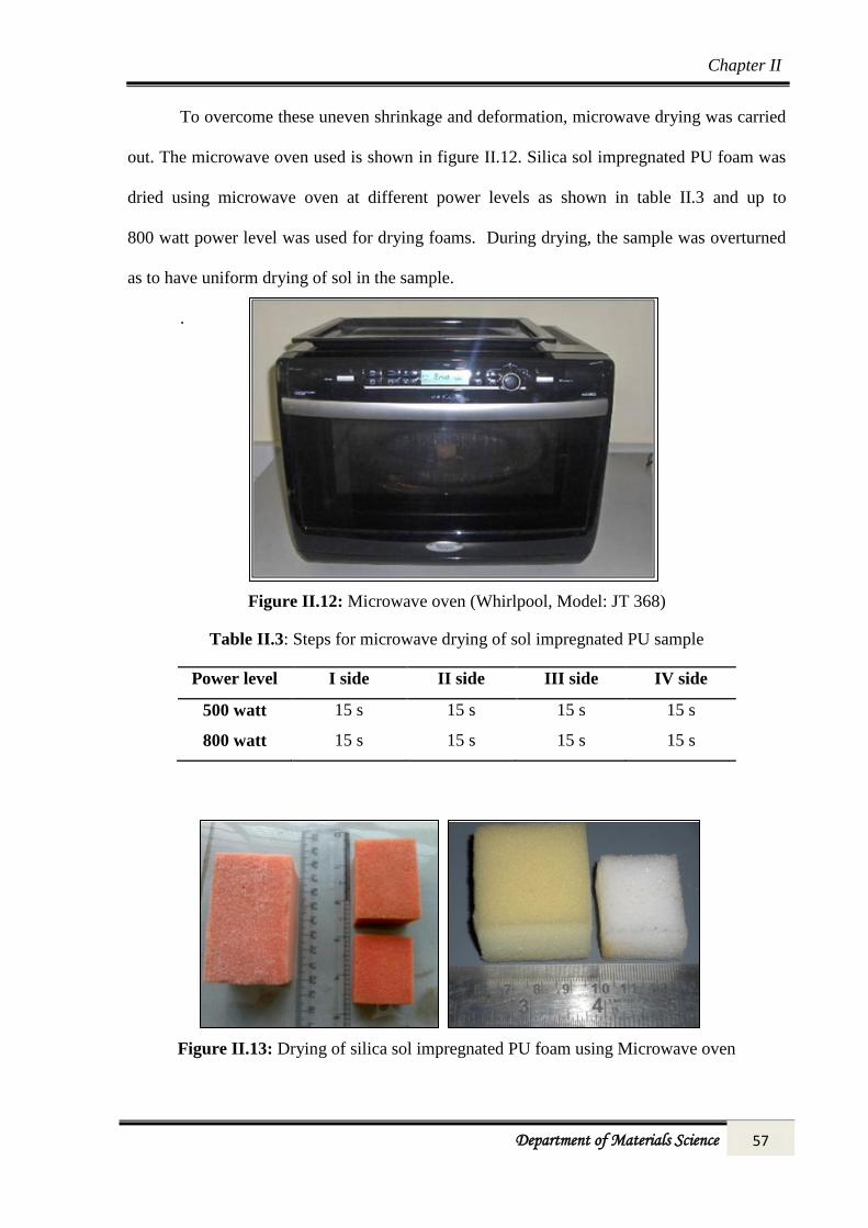
The surface area of carbon and silica foam was determined by BET surface area

analyzer (Micromeritics Gemini 2375) using nitrogen as adsorbent at 77 K shown in

figure II.20. Prior to adsorption, samples were degassed initially at 100°C for one hour in

presence of argon gas and at 250°C for 14 - 15 hours. After degassing sample was weighed

and attached to the surface area analyzer instrument. The nitrogen adsorption was studied at

liquid nitrogen temperature.

Figure II.20: BET Surface Area Analyzer (Micromeritics Gemini 2375).

Chapter II


II.4.2.2 Surface oxygen complexes:

The Boehm titration was used as a chemical method to quantitatively measure surface

oxygen groups present on carbon materials. It underlying theory says that bases of different

strength react with acidic surface functionalities present on the carbon samples. [1-3]

Accurately weighed 0.5 gm of the functionalized carbon foam samples was added to

250 ml Erlenmeyer flasks containing 50 ml of 0.1N NaHCO3, Na2CO3, NaOH and HCl

solution respectively. The flask was stoppered and stirred for 24 hours. After 24 hours of

stirring, solutions were filtered through a Whatman filter paper and excess of acid/base were

titrated with 0.1N base/acid solution.

The volume required for neutralization for a particular surface group was calculated

as follow:

NaHCO3 neutralizes carboxylic functionalities

Na2CO3 neutralizes carboxylic and lactone groups

NaOH neutralizes carboxylic, lactone and phenolic functionalities

HCl neutralizes basic groups present on surface

Total concentration of surface functionalities (Qe) available on carbon foam was

calculated by:

Where,

Ci = initial concentration (milimole)

Ce = final concentration (milimole) of corresponding acid/base,

V = volume of solution (ml),

Ms = weight of adsorbent (gm).

Chapter II


II.4.2.3 Surface groups (FTIR):

Functional groups present on foams at different heat treatment temperatures were

studied using Shimadzu FTIR-8300 Spectrophotometer shown in figure II.21. KBr was used

as reference material. Ratio between KBr to sample was kept 100:1. Before analysis KBr was

kept in oven at 110°C to remove the moisture. The fine ground sample was mixed with KBr

in agate mortar for uniform mixing. The sample was placed on sample holder of FTIR

instrument and spectra were obtained in range of 4000 to 400 cm-1

. The absorption peaks

observed on spectra were compared with standard literature data and analyzed for functional

groups. Area under the peak was calculated for different peaks using software provided with

the FTIR instrument.

Figure II.21: Infrared spectrophotometer (Shimadzu FTIR-8300)

II.4.3 Thermal properties

II.4.3.1 Thermal Gravimetric Analysis:

Thermal gravimetric analysis (TGA) was carried out using TGA, METTLER

TG/SDTA 851 as shown in figure II.22. Small piece of sample was cut and placed in vertical

furnace of TGA. Heating rate used in TGA was 15 ºC / min.

Chapter II


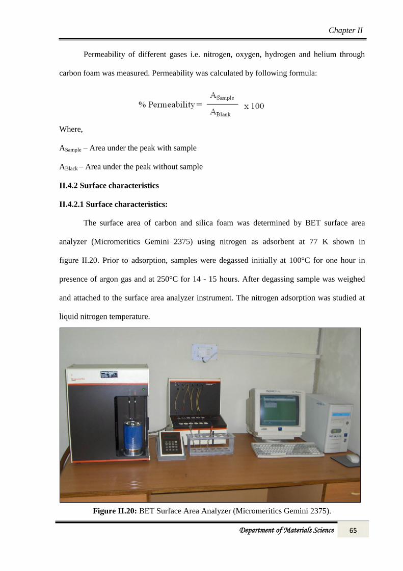
II.4.3.2 Specific Heat:

Specific heat was measured by using DSC, METTLER DSC20 along with Console

TC11 shown in figure II.23. Small piece of carbon foam was placed in crucible of differential

scanning calorimetric (DSC). The sample was heated from 80ºC to 600 ºC. Heating rate of

carbon foam during analysis was maintained at 15 ºC/min. The value of specific heat was

obtained from software available with instrument.

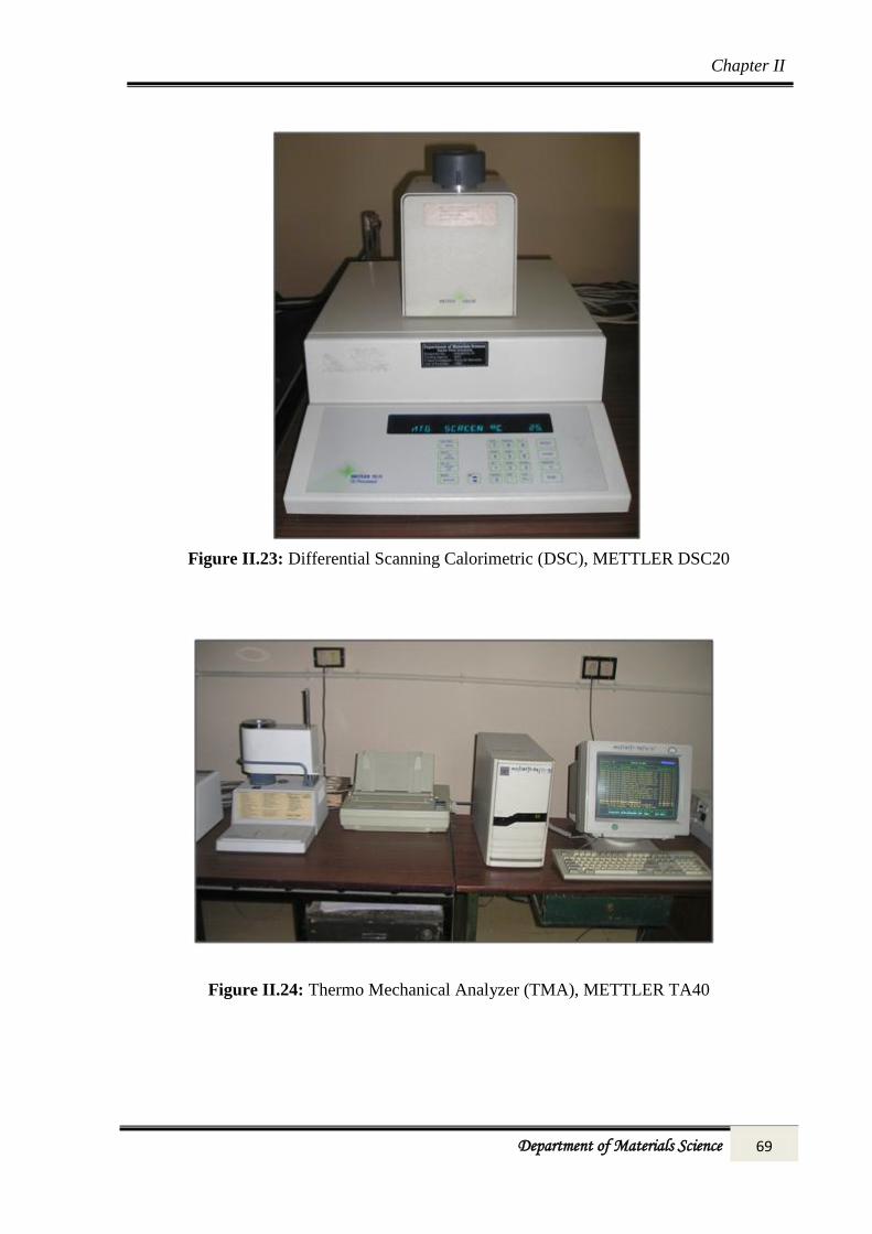
II.4.3.3 Co-efficient of thermal expansion:

Coefficient of thermal expansion (CTE) was measured by thermo mechanical analyser

(TMA), METTLER TA40 along with Console TC11 as shown in figure II.24. Carbon foam

sample was sandwiched between S.S. plate and heat treated at 800 °C. Heating rate during

testing was maintained at 15 ºC/min with nitrogen environment. CTE of carbon foam was

measured both cross sectional and transverse direction. Blank run was also performed using

standard S.S. plates.

Figure II.22: Thermo Gravimetric Analyzer (TGA), METTLER TG/SDTA851

Chapter II


Figure II.23: Differential Scanning Calorimetric (DSC), METTLER DSC20

Figure II.24: Thermo Mechanical Analyzer (TMA), METTLER TA40

Chapter II


II.4.4 Mechanical properties:

II.4.4.1 Compressive Strength:

Compressive strength is a measure of compressive load per unit area. Compressive

strength of carbon and silica foam was measured using Universal Testing Machine (UTM)

Shimadzu AG-100kNG shown in figure II.25. Load cell of 100 KN and crosshead speed of

1.5 mm/min were used. The sample having 25 x 25 x 25 dimensions were used for

measurement.

Figure II.25: Universal Testing Machine

Chapter II


II.4.5 Surface morphology

II.4.5.1 Scanning electron microscopy:

Surface morphology of PU foam, carbonized carbon foam and silica foam samples

were observed using Hitachi S-3000N as shown in figure II.26 Scanning Electron

Microscope. These samples were mounted on sample holder with the help of graphite tape.

The tape acts as both adhesive and conducting material. Specimens were scanned at different

magnifications. Non-conducting samples were coated with Pt-Pd in order to make conductive

samples.

Figure II.26: S-3000N Hitachi scanning electron microscope

Chapter II


II.4.5.2 Optical microscopy

Optical microscope was used to study the microstructure of PU foam for average pore

size, strut length and strut thickness having different density. The PU foams having different

densities were cleaned with distilled water, and cut into thin slice. The cleaned samples were

dried in oven at 100 oC. These dried samples were viewed under Leitz Optical Microscope at

different magnifications using polarized light as shown in figure II.27. The average pore size,

strut length and strut thickness was measured using LEICA image analysis software provided

with optical microscope.

Figure II.27: Leitz Optical Microscope

Chapter II


II.4.6 X-Ray Diffraction Analysis:

XRD analysis of carbon and silica foam were carried out by powder diffraction

method using X-Ray Diffractometer Philips, X’pert model shown in figure II.28 having

Cu Kα1 (λ-1.54056 Å) source. Fine powder of foam was pressed in stainless steel sample

holder. Wide angle X-ray diffraction patterns were recorded for analysis.

Figure II.28: X – Ray diffrectometer

Chapter II


II.4.7 Statistical analysis

Statistical analysis of carbon and silica foam was carried out using SPSS and

MINITAB data analysis software. Samples having different sizes were fabricated and

multiple regression tests were performed to generate linear equation to get idea of the

optimum shrinkage occurred in the sample after heat treatment.

Multiple linear regression (MLR) method is used to model linear relationship between

dependent variable and one or more independent variables. The dependent variable is

sometimes called predictand, and the independent variables as predictors. MLR is based on

least squares model. In the process of fitting or estimating model, statistics are computed that

summarize accuracy of regression model based upon selected condition. [4-10]

II.4.7.1 Model description:

In present work shrinkage was observed in length, breadth and thickness on heat

treatment of foam sample at 1000 °C in cured foam. Therefore, to carry out statistical

analysis and for modelling, data base was generated. For this, sample of foam of known

dimensions were taken and heat treated at 1000 °C under identical condition. The

dimensional shrinkage was measured for each and every sample. Using this data base

Multiple regression tests were performed on SPSS software to generate linear equation which

decides the optimum shrinkage for sample having any size.

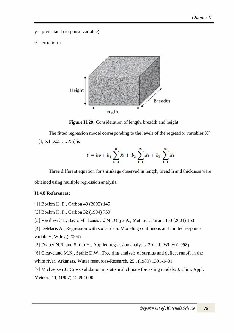
Model equation: The model expresses values of predicted variable as a linear function of

three predictor variables (i.e. shrinkage observed in length, breadth and thickness after heat

treatments shown in figure II.29) and an error term

Y = b0 + b1X1 + b2X2 + b3 X3 + e

Where,

X1, X2 and X3= value of predictor (length, breadth and thickness respectively)

b0, b1, b2 and b3 = regression constant (i.e. intercept)

Chapter II


y = predictand (response variable)

e = error term

Figure II.29: Consideration of length, breadth and height

The fitted regression model corresponding to the levels of the regressior variables X^

= [1, X1, X2, .... Xn] is

Three different equation for shrinkage observed in length, breadth and thickness were

obtained using multiple regression analysis.

II.4.8 References:

[1] Boehm H. P., Carbon 40 (2002) 145

[2] Boehm H. P., Carbon 32 (1994) 759

[3] Vasiljević T., Baćić M., Laušević M., Onjia A., Mat. Sci. Forum 453 (2004) 163

[4] DeMaris A., Regression with social data: Modeling continuous and limited responce

variables, Wiley,( 2004)

[5] Draper N.R. and Smith H., Applied regression analysis, 3rd ed., Wiley (1998)

[6] Cleaveland M.K., Stahle D.W., Tree ring analysis of surplus and deflect runoff in the

white river, Arkansas, Water resources-Research, 25:, (1989) 1391-1401

[7] Michaelsen J., Cross validation in statistical climate forcasting models, J. Clim. Appl.

Meteor., 11, (1987) 1589-1600

Chapter II


[8] Ostrom C.W., Jr., Time Series Analysis, Regression techniques, second edition:

Quantitative applications in the social sciences,: Newbury Park, Sage Publications., (1990)

07-009

[9] Weisberg S., Applied linear regression, 2nd ed. John Wiley, New York: 32416. Wilks,

(1985)

[10] Hogg R. And Craig A., Introduction to mathematical statistic, 4th edi., (1978) 192-95

[11] Hanushek E.and Jackson J, Statistical Methods for Social Scientists (1977) 110– 16

Experimental and Characterization Techniques II.1...

Documents

Transcript of Experimental and Characterization Techniques II.1...