Experimental Advances toward a Compact Dual-Species Laser Cooling...
96
Experimental Advances toward a Compact Dual-Species Laser Cooling Apparatus by Keith Ladouceur B.Sc., University of Guelph, 2004 A THESIS SUBMITTED IN PARTIAL FULFILMENT OF THE REQUIREMENTS FOR THE DEGREE OF Master of Science in The Faculty of Graduate Studies (Physics) The University of British Columbia (Vancouver, Canada) April, 2008 © Keith Ladouceur 2008
Transcript of Experimental Advances toward a Compact Dual-Species Laser Cooling...

Experimental Advances towarda Compact Dual-Species Laser
Cooling Apparatusby
Keith Ladouceur
B.Sc., University of Guelph, 2004
A THESIS SUBMITTED IN PARTIAL FULFILMENT OFTHE REQUIREMENTS FOR THE DEGREE OF
Master of Science
in
The Faculty of Graduate Studies
(Physics)
The University of British Columbia
(Vancouver, Canada)
April, 2008
© Keith Ladouceur 2008

Abstract
This thesis describes the advances made towards a dual-species magneto-optical trap(MOT) of Li and Rb for use in photoassociation spectroscopy, Feshbach resonancestudies, and, as long-term aspirations, the formation of ultracold heteronuclear polarmolecules. The initial discussion will focus on a brief theoretical overview of lasercooling and trapping and the production of ultracold molecules from a cold atomsource. Subsequently, details of the experimental system, including those pertainingto the required laser light, the vacuum chamber, and the computer control systemwill be presented. Finally, preliminary optimization and characterization measure-ments showing the performance of a single species Li MOT are introduced. Thesemeasurements demonstrated the loading of over 8×10⁷ Li atoms directly into a MOTwithout the need for a Zeeman slower.
ii

Table of Contents
Abstract . . . . . . . . . . . . . . . . . . . . . . . . . . . . . . . . . . . . . . ii
Table of Contents . . . . . . . . . . . . . . . . . . . . . . . . . . . . . . . . iii
List of Tables . . . . . . . . . . . . . . . . . . . . . . . . . . . . . . . . . . vi
List of Figures . . . . . . . . . . . . . . . . . . . . . . . . . . . . . . . . . . vii
Acknowledgements . . . . . . . . . . . . . . . . . . . . . . . . . . . . . . . xii
1 Introduction . . . . . . . . . . . . . . . . . . . . . . . . . . . . . . . . . 1
2 Principles of Laser Cooling and Trapping . . . . . . . . . . . . . . . 32.1 Scattering Force . . . . . . . . . . . . . . . . . . . . . . . . . . . . . 32.2 Dipole Force . . . . . . . . . . . . . . . . . . . . . . . . . . . . . . . 42.3 Optical Molasses . . . . . . . . . . . . . . . . . . . . . . . . . . . . . 62.4 MOT . . . . . . . . . . . . . . . . . . . . . . . . . . . . . . . . . . . 62.5 Magnetic Trap . . . . . . . . . . . . . . . . . . . . . . . . . . . . . . 92.6 Cooling Mechanisms . . . . . . . . . . . . . . . . . . . . . . . . . . . 10
2.6.1 Doppler Cooling limit . . . . . . . . . . . . . . . . . . . . . . 102.6.2 Sub-Doppler Cooling . . . . . . . . . . . . . . . . . . . . . . . 12
3 Ultra-Cold Molecules . . . . . . . . . . . . . . . . . . . . . . . . . . . . 153.1 Methods of Production . . . . . . . . . . . . . . . . . . . . . . . . . 153.2 Molecules from Cold Atoms . . . . . . . . . . . . . . . . . . . . . . . 16
3.2.1 Photoassociation . . . . . . . . . . . . . . . . . . . . . . . . . 163.2.2 Feshbach Resonance . . . . . . . . . . . . . . . . . . . . . . . 183.2.3 Electric Field Induced Feshbach Resonances . . . . . . . . . . 18
4 Laser Light . . . . . . . . . . . . . . . . . . . . . . . . . . . . . . . . . . 214.1 Requirements . . . . . . . . . . . . . . . . . . . . . . . . . . . . . . . 21
4.1.1 Lithium . . . . . . . . . . . . . . . . . . . . . . . . . . . . . . 214.1.2 Rubidium . . . . . . . . . . . . . . . . . . . . . . . . . . . . . 22
4.2 Master and Slave Lasers . . . . . . . . . . . . . . . . . . . . . . . . . 234.2.1 Master Locking Technique . . . . . . . . . . . . . . . . . . . . 244.2.2 Injection Locking of Slave Lasers . . . . . . . . . . . . . . . . 25
4.3 Photoassociation Laser . . . . . . . . . . . . . . . . . . . . . . . . . 264.4 Fiber Laser for Optical Dipole Trap . . . . . . . . . . . . . . . . . . 274.5 Ionization Laser . . . . . . . . . . . . . . . . . . . . . . . . . . . . . 27
iii

Table of Contents
5 Experimental Setup . . . . . . . . . . . . . . . . . . . . . . . . . . . . 285.1 Vacuum System . . . . . . . . . . . . . . . . . . . . . . . . . . . . . 28
5.1.1 Trapping Cell . . . . . . . . . . . . . . . . . . . . . . . . . . . 285.1.2 Vacuum Pumps . . . . . . . . . . . . . . . . . . . . . . . . . 29
5.2 Atomic Sources . . . . . . . . . . . . . . . . . . . . . . . . . . . . . . 315.2.1 Rubidium . . . . . . . . . . . . . . . . . . . . . . . . . . . . . 315.2.2 Lithium . . . . . . . . . . . . . . . . . . . . . . . . . . . . . . 31
5.3 Helmholtz and Compensation Coils . . . . . . . . . . . . . . . . . . . 325.3.1 Compensation Coils . . . . . . . . . . . . . . . . . . . . . . . 335.3.2 Helmholtz Coils . . . . . . . . . . . . . . . . . . . . . . . . . 33
5.4 Photoassociation Table . . . . . . . . . . . . . . . . . . . . . . . . . 345.5 Detection Methods . . . . . . . . . . . . . . . . . . . . . . . . . . . . 35
5.5.1 Fluorescence . . . . . . . . . . . . . . . . . . . . . . . . . . . 355.5.2 Absorption . . . . . . . . . . . . . . . . . . . . . . . . . . . . 36
5.6 RF State Selection . . . . . . . . . . . . . . . . . . . . . . . . . . . . 365.6.1 Lithium Antenna System . . . . . . . . . . . . . . . . . . . . 37
6 Control System Hardware . . . . . . . . . . . . . . . . . . . . . . . . . 416.1 Motivation . . . . . . . . . . . . . . . . . . . . . . . . . . . . . . . . 416.2 Hardware Components . . . . . . . . . . . . . . . . . . . . . . . . . . 41
6.2.1 The UTBus . . . . . . . . . . . . . . . . . . . . . . . . . . . . 416.2.2 Base Level Devices . . . . . . . . . . . . . . . . . . . . . . . . 436.2.3 Intermediate Level Devices . . . . . . . . . . . . . . . . . . . 466.2.4 High Level Devices (Actuators) . . . . . . . . . . . . . . . . . 54
7 Control System Software . . . . . . . . . . . . . . . . . . . . . . . . . 567.1 Design . . . . . . . . . . . . . . . . . . . . . . . . . . . . . . . . . . . 56
7.1.1 C++ Daemon . . . . . . . . . . . . . . . . . . . . . . . . . . 577.2 Control System Modules . . . . . . . . . . . . . . . . . . . . . . . . . 57
7.2.1 DDS module . . . . . . . . . . . . . . . . . . . . . . . . . . . 597.2.2 Analog Output Module . . . . . . . . . . . . . . . . . . . . . 617.2.3 Digital Output Module . . . . . . . . . . . . . . . . . . . . . 617.2.4 UTBus Device Module . . . . . . . . . . . . . . . . . . . . . . 627.2.5 Recipe Module . . . . . . . . . . . . . . . . . . . . . . . . . . 627.2.6 User Defined Experimental Scripts . . . . . . . . . . . . . . . 62
8 Measurements . . . . . . . . . . . . . . . . . . . . . . . . . . . . . . . . 658.1 MOT Optimization . . . . . . . . . . . . . . . . . . . . . . . . . . . 65
8.1.1 Alignment . . . . . . . . . . . . . . . . . . . . . . . . . . . . 658.1.2 Atom Number Calibration . . . . . . . . . . . . . . . . . . . . 658.1.3 MOT Loading Model . . . . . . . . . . . . . . . . . . . . . . 678.1.4 Detuning . . . . . . . . . . . . . . . . . . . . . . . . . . . . . 678.1.5 Intensity Dependence . . . . . . . . . . . . . . . . . . . . . . 708.1.6 Oven Current . . . . . . . . . . . . . . . . . . . . . . . . . . . 728.1.7 Conclusions . . . . . . . . . . . . . . . . . . . . . . . . . . . . 74
8.2 Ablation Loading . . . . . . . . . . . . . . . . . . . . . . . . . . . . . 74
iv

Table of Contents
8.2.1 Experimental Procedure . . . . . . . . . . . . . . . . . . . . . 748.2.2 Results . . . . . . . . . . . . . . . . . . . . . . . . . . . . . . 768.2.3 Conclusions . . . . . . . . . . . . . . . . . . . . . . . . . . . . 77
Bibliography . . . . . . . . . . . . . . . . . . . . . . . . . . . . . . . . . . . 80
v

List of Tables
8.1 Natural linewidths and values of s = I/Isat for the atomic species usedin our experiment. . . . . . . . . . . . . . . . . . . . . . . . . . . . . 67
8.2 Intensities of Pump and Repump Beams in each axis with primaryand reflected beam transmission factors for both s and p polarizations.The transmission coefficient determines the intensity value of the lightwhen it reaches the MOT. . . . . . . . . . . . . . . . . . . . . . . . . 72
8.3 Loading rate and loss rates for ablation loading trials on surface A. . 76
vi

List of Figures
2.1 Absorption and spontaneous emission process for an atom with initialvelocity v. (a) A photon of momentum hk is absorbed by an atom;(b) The atom has been slowed by hk/m; (c) Spontaneous emission ofa photon in a random direction. . . . . . . . . . . . . . . . . . . . . . 4
2.2 A two-level atom in the presence of a red detuned electric field. (a)The energy levels of the atomic states are driven in opposite directions;(b) The presence of a spatially homogeneous field generates a minimain the potential, allowing for atoms to be trapped. . . . . . . . . . . . 5
2.3 Counter-propagating laser fields red detuned from an atomic transi-tion. Left An atom at rest does not absorb photons from either beam;Right An atom with velocity v will preferentially absorb photons fromthe beam Doppler shifted to resonance. . . . . . . . . . . . . . . . . . 7
2.4 Schematic diagram showing the polarizations and directions of thecooling light in a magnetic trap. . . . . . . . . . . . . . . . . . . . . . 8
2.5 Diagram showing the hyperfine splitting of the excited atomic state inthe presence of a linearly varying magnetic field in one-dimension. Thissplitting is the origin of the position dependent force in a magneto-optictrap. . . . . . . . . . . . . . . . . . . . . . . . . . . . . . . . . . . . 8
2.6 Schematic diagram demonstrating the method of gradient cooling. Asthe atom reaches the peak potential, it is driven to the lower energystate by optical pumping. The energy difference is released as a spon-taneously emitted photon. . . . . . . . . . . . . . . . . . . . . . . . . 12
3.1 Photoassociation method for producing ultracold molecules. (a) Aphoton of sufficient energy couples with a free atom pair during acollision event, generating a bound excited state molecule. (b) Themolecule quickly decays back into its constituent atoms. These atomsoften gain kinetic energy during this process and exit the trap. (c) Asecond photon may drive the transition from the upper excited stateto a lower ground state. Careful tuning of this second photon mayallow for the production of vibrationally cold ground state molecules. 17
3.2 Increasing magnetic field strength drives the closed channel closer inenergy to the open channel. A Feshbach resonance occurs for a mag-netic field at which these two channels become degenerate. . . . . . . 19
vii

List of Figures
3.3 High DC voltage electrodes for use in the electric field induced Fes-hbach resonance experiment. The electrodes are attached to a 1.33”vacuum CF flange electrical feedthrough. Inserted into the vacuumchamber, the extended length will allow the electrodes to be placedphysically close to the trapping region of the atomic gas. The spacingof the electrodes is approximately 1.3mm. . . . . . . . . . . . . . . . 20
4.1 Energy level diagram of 6Li with 7Li shown for comparison. The cool-ing and repump light transitions are shown. [1] . . . . . . . . . . . . 22
4.2 Energy level diagrams for 85Rb and 87Rb with the corresponding cool-ing and repump transitions shown.[1] . . . . . . . . . . . . . . . . . . 23
4.3 Schematic representation of the Littrow configuration used as a feed-back mechanism for the master laser diodes. The grating and mirrorare monolithic and move as a single entity in order to minimize thetranslation of the output beam as the grating angle and cavity are varied. 24
4.4 Sample error signal (shown in black) derived from the saturated ab-sorption spectrum (shown in blue) for 6Li. The laser frequency islocked to the zero crossing of the error signal. . . . . . . . . . . . . . 26
5.1 Simplified view of the vacuum system including positions of the ionand NEG pumps, as well as the glass trapping cell. . . . . . . . . . . 29
5.2 Direct view of the atomic sources used within the experiment. At-tached to a UHV feedthrough, the Rb atoms are dispensed by wayof a temperature dependent chemical reaction while the Li atoms areemitted from the effusive oven as the metal is heated above its meltingpoint. . . . . . . . . . . . . . . . . . . . . . . . . . . . . . . . . . . . 32
5.3 Schematic diagram depicting the procedure for creating the necessaryfrequency locked light on the Master table. The light is then sent tothe Photoassociation experiment via fiber optical cables where it isfurther frequency shifted and amplified before being introduced to theMOT chamber. . . . . . . . . . . . . . . . . . . . . . . . . . . . . . . 35
5.4 The photodiode fluorescence imaging system. The light for both atomicspecies is imaged independently on PD1 and PD2 through the use ofa dichroic mirror and two interference filters (IF1 and IF2).[2] . . . . 36
5.5 Frequency dependence of the radiated power, as measured by a one-loop pick-up coil, of the two RF state selection antennas. The an-tennas are driven by an amplified signal directly from a DDS device.The sharp decline in output power of the ‘Key Hole’ antenna at lowfrequencies necessitated a dual antenna system. . . . . . . . . . . . . 37
5.6 Determination of the radiated power of the dual antenna system athigh frequencies measured by a one-loop pick-up coil on axis at a dis-tance R from the center of the coils. The antennas are driven by anamplified, frequency doubled DDS signal. . . . . . . . . . . . . . . . . 38
viii

List of Figures
5.7 Schematic diagram showing the dual antenna implementation for RFstate selection. The coil antenna is used to drive hyperfine groundstate transitions below 40MHz, while the ‘Key Hole’ antenna is usedto drive transitions at 228MHz. . . . . . . . . . . . . . . . . . . . . . 39
5.8 Schematic diagram showing the signal generation of the microwavestate selection system. A single voltage controlled oscillator (VCO) isused to produce the necessary frequencies for both Rb isotopes. Theimplementation of an antenna to couple these fields has yet to be realized. 40
6.1 Conceptual representation of the UTBus output. Each instructionsent across the bus is received by all devices, but only the one with amatching address allows the data to be latched. . . . . . . . . . . . . 42
6.2 Timing diagram showing the latching of data to a device in relation tothe strobe signal. Instructions are sent three times across the UTBus,with the strobe set low, to high, and back to low before a new instruc-tion is likewise sent. This modulation of the strobe ensures that thedata is properly latched and settled before the next instruction update. 43
6.3 Configuration of the 50-pin UTBus connector. The cable and con-nectors support data transmission over long distances (20ft) and arereadily available from most electronic suppliers.[3] . . . . . . . . . . 44
6.4 During the initial design, the ACK2 line was intended for use as thestrobe signal output. However, this proved difficult to control from thesoftware system, so instead the DIOD0 line was rewired for use as thestrobe signal line. . . . . . . . . . . . . . . . . . . . . . . . . . . . . . 45
6.5 Frequency response of the DDS amplification system. The amplitudeof the DDS decreases linearly as the frequency approaches the cutoffof the low pass filter of the cosine output. The response of the pre-amplifier and amplifier show non-linear variations. . . . . . . . . . . . 47
6.6 Amplitude response of the DDS amplification system. . . . . . . . . . 486.7 Top level PCB layout of the modified DDS device. The functionality of
individual units can be tailored for a specific requirement by changingthe location of 0Ω jumpers. . . . . . . . . . . . . . . . . . . . . . . . 49
6.8 A broken connection to the power inputs of two integrated circuitson the Analog Output devices required the addition of small wires tobridge the gap. . . . . . . . . . . . . . . . . . . . . . . . . . . . . . . 51
6.9 Strobe function settings for DDS device[3] . . . . . . . . . . . . . . . 536.10 Output select settings for the Analog Output where XXXXX refers to
the device address[4] . . . . . . . . . . . . . . . . . . . . . . . . . . . 536.11 Addressing hierarchy for the QDG control system. This is necessary
due to the variations in how the 8-bit address of the UTBus is used toaccess specific devices. This addressing method ensures that no twodevices will be updated during the same clock cycle . . . . . . . . . . 54
ix

List of Figures
7.1 Schematic showing the Control System hierarchy. A user written con-trol script is written in Python. Bytecode is generated and passed tothe C++ Daemon, which in turn updates the NI-DAQ card and writesthe instruction stack to the onboard memory. The NI-DAQ sends asingle instruction across the UTBus every clock cycle. The instruc-tions update the state of a specific device on the bus. The state of thedevice determines the output, which is in turn used to drive the stateof an experimental actuator. . . . . . . . . . . . . . . . . . . . . . . . 58
7.2 Module schematic showing the relation between the major componentsof the QDG Computer Control Program. . . . . . . . . . . . . . . . . 59
8.1 The relationship between the fluorescence signal from the CCD cameraand the photodiode. The photodiode signal has been calibrated withthe atom number; a linear fit allows for the camera signal to be likewiseconverted. . . . . . . . . . . . . . . . . . . . . . . . . . . . . . . . . . 66
8.2 Fluorescence from a CCD camera was recorded every 500ms over theduration of the loading period of a Li MOT. The fluorescence wasconverted to atom number and fit using equation (8.5). The values ofthe parameters were found to be R = 1.1 × 10⁶ and γ = 0.054. Thiscorresponds to a loading time of τ = 18.2sec. . . . . . . . . . . . . . . 68
8.3 Atom number vs. laser detunings for increasing values of the magneticcoil current (Icoil). The coil current is proportional to the magneticfield gradient. Note the shift of the maximum atom number towardshigher detuning values as the current is increased. The peak atomnumber of 2.61× 10⁷ atoms is found at δp = −42MHz, δr = −44MHz,and Icoil = 7A. For our experiment a reference current of 2.84A wasmeasured to produce a magnetic field of 16.8G/cm. . . . . . . . . . . 69
8.4 Sample contour plots at Icoil = 4A showing the raw fluorescence datafor both the CCD camera signal and the photodiode signal. . . . . . . 70
8.5 Clockwise from top: (a) Contour plot showing the atom number presentin the MOT as a function of the light intensity of the pump and re-pump beams. (b) Increasing atom number for fixed pump power. (c)Increasing atom number for fixed repump power . . . . . . . . . . . 71
8.6 Fluorescence measurements and loading times determined as a func-tion of oven current for multiple compensation z-coil voltages. Thesevoltages correspond to currents, which in turn correspond to magneticfields. These magnetic fields determine the MOT position within thetrapping cell. Higher oven currents result in a larger flux of atoms, butwith an increased shift in the velocity profile. Altering the voltage tothe compensation z-coil shifts the MOT position relative to the centerof the trapping field and was done to observe the effect of the beamblock. . . . . . . . . . . . . . . . . . . . . . . . . . . . . . . . . . . . 73
x

List of Figures
8.7 The adsorbed Lithium layer is present on all sides of the trapping cell,extending in a thin layer approximately 9mm past the position of thebeam block. Ablation loading was tested first by directing the pulsedYAG light on the Lithium-Vacuum interface at the bottom of the cell(A), then by directing it on the Glass-Lithium interface at the top ofthe cell (B). . . . . . . . . . . . . . . . . . . . . . . . . . . . . . . . 75
8.8 Top: A Li MOT is loaded by means of laser ablation at the interfaceof the vacuum-Lithium layer, as well as from an effusive oven source.The laser is triggered at the 5 second mark. Bottom: Increased viewof the loading and decay curves of the laser ablation trials. The beampositon was held fixed throughout. The laser light is turned off 60seconds after being triggered. The decay time for each of the threetrial are calculated to be τ1 = 118.2s, τ2 = 120.3s, and τ3 = 119.2s. . 78
8.9 Top: A Li MOT is loaded by means of laser ablation at the glass-Lithium layer interface. Shown are the loading and decay periods formultiple trials at a single beam location. The laser light was triggeredat the 5 second mark, and turned off 60 seconds later. The depletionof the deposition layer is significant as the atom number of the finaltrial is nearly nonexistent. The decay rate of the trapped atoms afterthe YAG light has been turned off is τ = 14.5s. Bottom: A shorttime scale view of the initial loading conditions. The early spike in theatom number is maintained over four images at 500ms intervals. Thelaser is pulsed at 10Hz. . . . . . . . . . . . . . . . . . . . . . . . . . . 79
xi

Acknowledgements
The contributions discussed within this thesis are really a very small part of a muchlarger whole; as such I owe a great amount of gratitude to all those I’ve had the plea-sure of working with. Their knowledge and dedication are the reason this experimenthas progressed so far. To this end I’d like to thank my supervisor, Dr. Kirk Madison,for everything that he has taught me. Dr. David Jones for his perspective and advice.Dr. Bruce Klappauf for patiently ignoring the inanity of my many questions, andJanelle Van Dongen for her pragmatic approach to experiment. Further, I’d like tothank Dr. Art Mills, Dr. Jim Booth, and Swati Singh for their contributions andconversation. To the great many others who I have had the honour of working with,the list is becoming too long to write, know that your insights and friendships havebeen very much appreciated.
On a more personal side, I would like to thank my family, and in particular myparents, for their for their ever present love and support. It is a great comfort to knowthat, regardless of my path in life, they are always there to offer encouragement.
Finally, I would like to thank my very patient and understanding girlfriend KatieDinelle. She has been a source of strength from the beginning, and I could not haveseen this to the end without her.
xii

Chapter 1
Introduction
The term ‘ultracold’ is used to describe temperature regimes below 1µK[5]. At suchlow temperatures, the subtle many-body quantum effects that are normally sup-pressed at high temperatures become extremely important. The idea that atomscould be cooled through the use of laser radiation was first proposed by Hansch andSchawlow [6] in 1975. From this inception, methods of laser cooling and trapping weresteadily developed and refined — culminating in 1995 with the first demonstrationsof Bose-Einstein condensation in Rubidium[7] and Cesium[8]. These demonstrationsshowed that the techniques used for cooling and trapping atoms had matured; witha clear experimental path, access to dense samples of ultracold atoms intensifiedinterest and further spurred theoretical and experimental research.
The progression from atoms to molecules is a natural one. The additional internalstructure and anisotropic interactions present in molecules make their study a farmore intriguing proposition. Unfortunately, this added complexity precludes thesimple extension of laser cooling techniques to a source of hot molecules. Undeterred,researchers instead developed methods of forming molecules from a prepared sampleof ultracold atoms. These methods include photoassociation, where the free states ofa colliding atomic pair are coupled to a vibrationally excited bound molecular stateby the introduction of a resonant photon, and Feshbach resonance, where degeneracyof the atomic and molecular states is achieved by tuning an applied magnetic field.The availability of cold, stable molecules in the vibrational ground state are criticalin furthering research across many areas of physics and chemistry.
Of particular interest are heteronuclear polar molecules, such as LiRb, as theyare characterized by a permanent electric dipole moment. This dipole moment, atultracold temperatures where the thermal energy of the molecules is low, can be con-trolled by an applied electric field. Possible applications include the implementationof polar molecules in a lattice as a quantum computation device [9], where a qubitis represented by the alignment of the dipole with or against an electric field. Thefull depth and breadth of ultracold physics has yet to fully realized, and although thetechnical difficulties of generating such systems are great, the possible rewards areextremely tantalizing.
The research being conducted within the Quantum Degenerate Gas (QDG) Lab-oratory is concerned with many of the aspects of these ultracold systems, and assuch is quite extensive in its scope. The aim of the project from its inception wasto build a modularized infrastructure capable of supporting multiple experiments fo-cused on the study and manipulation of 85,87Rb and 6Li in cold and ultracold atomicand molecular states. Alkali atoms are used most prevalently within ultracold exper-iments as the single valence electron leads to a simplified energy structure, while theenergy difference between the internal states is accessible by optical and near infra-
1

Chapter 1. Introduction
red light. The high vapour pressure of Rubidium allows for loading from an atomicvapour, while the lower pressure of Lithium requires an effusive oven to generate anatomic source. As a foundation for this infrastructure, an isolated master table wasbuilt for generating, locking, and conditioning the light necessary for all species andisotopes. The design of the amplification systems, vacuum chambers, and trappingcells were generalized for use within multiple experimental systems; small deviationsfrom a basic plan would differentiate an experiment probing Feshbach resonancesfrom one concerned with photoassociation spectroscopy. The control system, neces-sary in such experiments where the timing of the state change of individual devicesis critical, was to be developed as a powerful, fully realized method of supportingprecise experimental sequencing for data collection.
The following discussion will be focused on the development of this system; therelevant theoretical background, the experimental developments toward a dual-speciesMOT, and early performance results of the apparatus in a single species Li MOTconfiguration will be shown. A project of this scope is by necessity long term innature, as such what I present is merely the state of the apparatus in its current formand not as a finished product.
2

Chapter 2
Principles of Laser Cooling andTrapping
The interaction of light with matter is fundamental in cooling and trapping densesamples of atomic gases. The mechanical force resulting from this interaction isderived from two basic mechanisms; the scattering force and the dipole force.
2.1 Scattering Force
The scattering force is most naturally developed by considering light as a particle.During the absorption of a photon by an atom, conservation requirements dictatethat the atom experiences a momentum shift of hk where k is the wave vector ofthe incoming photon. The excited atom is unstable and will decay back to theground state through spontaneous emission. The direction of the outgoing photonis determined by the radiation pattern of the transition. Solving the optical Blochequations for a two-level atom in the presence of a radiation field results in thefollowing expression for the average scattering force [10]
Fscatt = hkΓ
2
(Ω2/2
δ2 + (Γ2/4) + (Ω2/2)
)= hkγS (2.1)
where Γ is the natural linewidth of the excited state, δ = ω−ωO+k·v correspondsto the detuning of the photon frequency from the atomic resonance with the Dopplershift of the atom taken into account, Ω is the characteristic Rabi frequency of theatom-field interaction, and γS is the spontaneous scattering rate.
The Rabi frequency and the natural linewidth are related to the saturation inten-sity by
I
Isat=
2Ω2
Γ2(2.2)
where Isat = πhc/3λ3τ , and τ is the decay time for the transition. Introducing thisrelation to (2.1)
Fscatt = hkΓ
2
(I/Isat
1 + (I/Isat) + (4δ2/Γ2)
)(2.3)
At high light intensities, this equation reduces to Fmax = hkΓ/2. The rate of spon-taneous emission from a two level atom approaches Γ/2 because the populations inthe upper and lower states both approach 1/2.
3
Chapter 2. Principles of Laser Cooling and Trapping
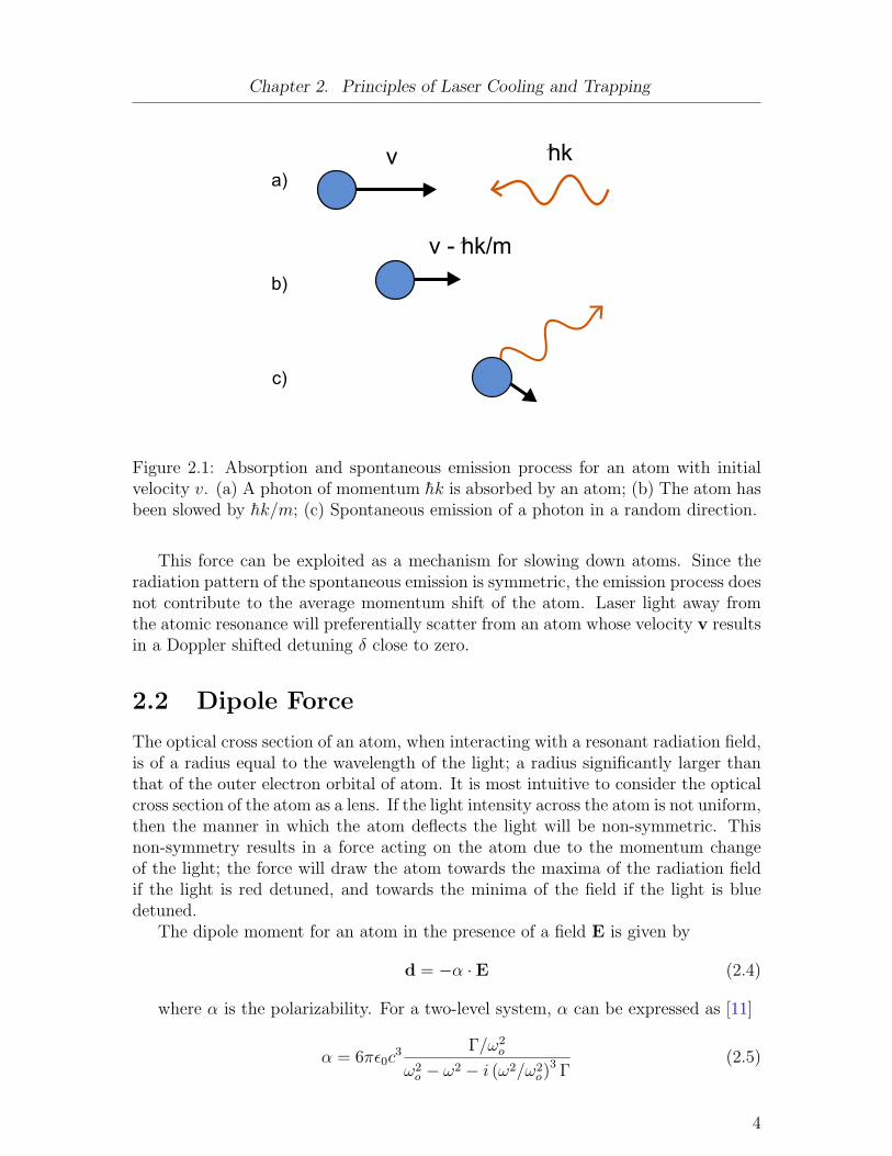
Figure 2.1: Absorption and spontaneous emission process for an atom with initialvelocity v. (a) A photon of momentum hk is absorbed by an atom; (b) The atom hasbeen slowed by hk/m; (c) Spontaneous emission of a photon in a random direction.
This force can be exploited as a mechanism for slowing down atoms. Since theradiation pattern of the spontaneous emission is symmetric, the emission process doesnot contribute to the average momentum shift of the atom. Laser light away fromthe atomic resonance will preferentially scatter from an atom whose velocity v resultsin a Doppler shifted detuning δ close to zero.
2.2 Dipole Force
The optical cross section of an atom, when interacting with a resonant radiation field,is of a radius equal to the wavelength of the light; a radius significantly larger thanthat of the outer electron orbital of atom. It is most intuitive to consider the opticalcross section of the atom as a lens. If the light intensity across the atom is not uniform,then the manner in which the atom deflects the light will be non-symmetric. Thisnon-symmetry results in a force acting on the atom due to the momentum changeof the light; the force will draw the atom towards the maxima of the radiation fieldif the light is red detuned, and towards the minima of the field if the light is bluedetuned.
The dipole moment for an atom in the presence of a field E is given by
d = −α · E (2.4)
where α is the polarizability. For a two-level system, α can be expressed as [11]
α = 6πε0c3 Γ/ω2
o
ω2o − ω2 − i (ω2/ω2
o)3 Γ
(2.5)
4

Chapter 2. Principles of Laser Cooling and Trapping
Figure 2.2: A two-level atom in the presence of a red detuned electric field. (a) Theenergy levels of the atomic states are driven in opposite directions; (b) The presenceof a spatially homogeneous field generates a minima in the potential, allowing foratoms to be trapped.
As before, ωo is the frequency, and Γ the natural linewidth of the ground to excitedstate transition. The interaction potential of the induced dipole moment with thelight field E is then
Udip = −1
2d · E = −1
2ε0cRe(α)I (2.6)
and the dipole force simply
Fdip = −∇Udip =1
2ε0cRe(α)∇I (2.7)
For large detunings (|δ| Γ) and high intensities (where |δ| Ω) the rotatingwave approximation becomes valid. The interaction potential and scattering ratereduce to
Udip 'hΩ2
4δ≡ hΓ
8
Γ
δ
I
Isat(2.8)
Γscatt 'Γ
8
Γ2
δ2
I
Isat(2.9)
where δ = ω − ωo. As described earlier, and now shown explicitly, a positivedetuning results in a decreasing potential from the region of highest intensity, whilea negative detuning results in a trapping potential. It is important to note that atsuch large frequency detunings, the scattering rate has a I/δ2 dependence while thetrap depth is proportional to I/δ. This means that it is possible to create a trap thatis sufficiently deep to confine atoms while keeping the scattering rate low to reducespontaneous scattering; the result is a conservative potential for which the atom doesnot change its internal state.
5

Chapter 2. Principles of Laser Cooling and Trapping
2.3 Optical Molasses
An optical molasses is an arrangement of three orthogonal sets of counter-propagatinglight fields such that an atom within the intersection of the fields is subject to areduction in velocity regardless its direction of movement. If we focus solely onthe beams propagating in the +x and −x directions, the equation describing thescattering force (2.1) for an atom travelling opposite to the direction of the beambecomes
F+ = hkγ
2
(I/Isat
1 + I/Isat + (δo + kv)2 /Γ2
)(2.10)
for a beam propagating in the same direction as the atom, where δo = ω − ωo, and
F− = −hkγ
2
(I/Isat
1 + I/Isat + (δo − kv)2 /Γ2
)(2.11)
An atom at rest will have no net force acting on it, as the two beams (assumingidentical frequencies and intensities) will cancel. However, if the atom is moving withsome velocity v then the forces will no longer balance. Further, if the velocity of theatom is such that |kv| Γ and |kv| |δo|, then the total force acting on the atomis approximated by [12]
Fmolasses = 4hk2 I
Io
2δΓv[1 + (2δ/Γ)2
]2 (2.12)
where terms of order (kv/Γ)4 and higher have been neglected. If the detuning δo isless than zero, then the force will oppose the velocity of the atom. This results in adamping force on the atom similar to the force on a particle in a viscous fluid. Thissimilarity is what originally led to the appellation of the ’Optical Molasses Technique’[13].
2.4 MOT
An optical molasses will cool atoms; however, the atoms are free to exit from theregion where the cooling beams intersect. Removed from this region, the atomsare no longer accessible to the laser light until they once again reenter the beampath by way of diffusion. In order to trap the beams within the cooling region,an inhomogeneous magnetic field is applied in such a way as to combine with thelight beams to produce spatial confinement by way of a position dependent radiationpressure. This arrangement is known descriptively as a magneto-optical trap (MOT)and was first demonstrated in three dimensions in 1987 Raab et al. [14].
A magnetic field with a constant gradient is overlaid with the counter propagat-ing, circularly polarized cooling beams described in the optical molasses section. Themagnetic field is produced by way of two magnetic coils in an anti-Helmholtz config-uration (the direction of current flow in one coil is opposite that of the other coil),such that there exists a zero field at the intersection of the cooling beams with a
6

Chapter 2. Principles of Laser Cooling and Trapping
Figure 2.3: Counter-propagating laser fields red detuned from an atomic transition.Left An atom at rest does not absorb photons from either beam; Right An atomwith velocity v will preferentially absorb photons from the beam Doppler shifted toresonance.
radially increasing, linear magnetic field away from the center. In this configuration,the Zeeman shift of the electronic levels of the atom are dependent on the positionof the atom within the trap.
In order to understand the mechanism underlying this trapping scheme, a two-level atom travelling in the +x direction with a J = 0 −→ J = 1 transition isconsidered. The Zeeman shifts of the electronic levels due an applied magnetic fieldB(z) are
∆wB =µBh· dBdx· x (2.13)
where µB is the Bohr magneton. This atom is also in the presence of two counter-propagating laser beams along the ±x directions with the same circular polarizations.The direction of the beam propagation with respect to the magnetic field is whatdrives the σ− transition of an atom moving in the +x direction, and the σ+ of anatom moving in the −x direction. Incorporating both the force due to the Dopplershift, as well as the force due to the Zeeman shift gives
F− = − hk2
ΓI/Isat
4(δo + kv + µB
h· dBdx· x)2
+ I/Isat + 1(2.14)
The reverse is true for an atom propagating in the −x axis.
F+ =hk
2Γ
I/Isat
4(δo − kv − µB
h· dBdx· x)2
+ I/Isat + 1(2.15)
For small velocities and displacements, the total restoring force acting on an atomcan be given by
7

Chapter 2. Principles of Laser Cooling and Trapping
Figure 2.4: Schematic diagram showing the polarizations and directions of the coolinglight in a magnetic trap.
Figure 2.5: Diagram showing the hyperfine splitting of the excited atomic state inthe presence of a linearly varying magnetic field in one-dimension. This splitting isthe origin of the position dependent force in a magneto-optic trap.
8

Chapter 2. Principles of Laser Cooling and Trapping
FMOT = −αv −Kx (2.16)
where α is the damping constant, corresponding to the frictional force responsiblefor the optical molasses, and K is the spring constant of the damped harmonic os-cillator, resulting in a position dependent restoring force to the zero of the magneticfield. This one-dimension derivation can be expanded to include all three Cartesianaxes, although in three dimensions there is required further discussion of the exactnature of the cooling and loss mechanisms responsible for the bounds on the ensembletemperature and number.
2.5 Magnetic Trap
A MOT is essential for the initial cooling and trapping of free atoms, but it is notalways the most convenient environment for probing an ultracold atomic gas due tothe constant variation in the internal state of the atoms.
A magnetic dipole µ in the presence of a magnetic field has potential energy
V = −µ ·B (2.17)
for an atom in a state |IJFmF 〉 the Zeeman energy is given by
V = gFµBmFB (2.18)
This result is the basis for magnetic trapping. The potential of the atom is only de-pendent on the magnitude of the field at any given position, and not on the direction.The reason is that as the atom moves throughout the trapping region, the atomicdipole adiabatically rotates to maintain an alignment with the magnetic field. Fromthis, the force on the atom is simply
F = −gFµBmF∇B (2.19)
The spin dependence of the force means that, depending on the sign of gF , apositive spin state will experience a trapping potential, while a negative spin statewill be expelled from the trapping region and lost to the ensemble. For an initialMOT of F = 1/2 atoms with equally populated hyperfine states, this results in aninitial loss of approximately 50% in the atom number.
The field for the magnetic trap can be created by the same coils used to producethe magnetic field in the MOT. The MOT coils are implemented in an anti-Helmholtzconfiguration, producing a quadrupole magnetic field. This field has the disadvantageof producing a vanishing field at the center of the trap. In this region, the energyspacing of the atomic hyperfine states is negligible (the spacing being of order µBB)and a pronounced mixing of the magnetic quantum states occur. This results inan appreciable transfer of atoms from the trapped mF > 0 states to the untrappedmF < 0 states. Atoms transferred in this way are quickly expelled from the trap.There are various methods available to compensate for this loss mechanism. It ispossible to lift the average potential of the trap center by applying an oscillating
9
Chapter 2. Principles of Laser Cooling and Trapping
bias field to the system. Known as a TOP trap, this method was used in the firstsuccessful Bose-Einstein condensation experiments. It is also possible to expel atomsfrom the center of the trap using an applied laser field.
Magnetic trapping is used to increase the density of the laser cooled atoms inorder to achieve high collision rates necessary for efficient evaporative cooling [15].
2.6 Cooling Mechanisms
The Doppler cooling method is the most important in the preparation of cold, trappedatoms from a hot atomic source [16]. Although there is a theoretical lower boundon the temperature attainable using this technique, further cooling mechanisms areavailable that remove this limitation The Doppler cooling limit, as well as the sup-plementary cooling techniques used within our experiment will be discussed.
2.6.1 Doppler Cooling limit
The force on an atom from a single laser beam can be written as
F = Fabs + δFabs + Fspont + δFspont (2.20)
Clearly, the scattering force corresponds to the average force from the absorptionof a photon, and the net force from spontaneous emission must average to zero dueto symmetry considerations. What must be considered is the effect of the smallfluctuations δFspont and δFabs on the internal energy of the atom.
Each emission event alters the state of the atom by some recoil velocity vr = hkm
,where k is the wave-vector of the photon emitted. Similar to the Brownian motion ofpollen in a liquid, the atom undergoes a random walk in its velocity due to the randomnature of the emission process. After N emission events, the mean displacement invelocity space is proportional to
√N [12]. During a time t the average emission events
isN = Γscattt (2.21)
and the mean-square of the velocity in one of the three Cartesian coordinates willincrease as
v2spont = ηv2
rΓscattt (2.22)
The factor η = 〈cos2 θ〉 is the angular average. For a completely isotropic emissionpattern η = 1/3.
Absorption events due not occur uniformly in time. Since each absorption eventis followed by spontaneous emission, the mean number of photons absorbed in timet is also given by (2.21). However, if it is assumed that the events follow a Poissondistribution, then there will exist a one-dimensional random walk in the velocityalong the laser beam in conjunction with the change in velocity due to the meanforce. Since all the photons have a common k vector, the factor η is unity.
v2abs = v2
rΓscattt (2.23)
10
Chapter 2. Principles of Laser Cooling and Trapping
Now, employing Newton’s second law it is possible to rewrite (2.20) in terms of theaverage velocities of the individual mechanisms
d
dt
(1
2mv2
)=
d
dt
1
2m(v2abs + v2
spont + v2scatt
)(2.24)
Incorporating (2.22) and (2.23) gives
d
dt
(1
2mv2
)=
1
2m
(v2rΓscatt + ηv2
rΓscatt + 2vscattd
dtv
)(2.25)
and the addition of a counterpropagating beam gives
d
dt
(1
2mv2
)= mv2
r(1 + η)Γscatt + vFmolasses (2.26)
This describes the balance between the contributions of the optical molasses to-wards cooling, and the contributions of the fluctuations towards heating. Assumingthat the light fields are symmetric (this isotropy gives the value of η as one) and thatthe intensities are far from saturation (allowing for the assumption that the scatteringrate of the atom is six times as the rate for a single beam), the extension to a threedimensional optical molasses results in
d
dt
(1
2mv2
)= 2mv2
rΓscatt + αv2 (2.27)
In the cooling limit, the net force on the atom must be zero. The equilibriumstate for each of the three axes is then given by
v2 = 2mv2r
Γscattα
(2.28)
According to the equipartition theorem, the kinetic energy of the atom is related tothe temperature by
1
2mv2 =
1
2kBT (2.29)
Using the above relation, as well as the previously derived values for α and Γscatt,allows for an expression for the temperature to be written
kBT =hΓ
4
1 + (2δ/Γ)2
(−2δ/Γ)(2.30)
It is straightforward to show that the minimum temperature occurs for a detuningof half the natural linewidth to the red (δ = −Γ/2).
kBTD =hΓ
2(2.31)
This result is the lowest temperature achievable in an optical molasses with a two-level atom and is referred to as the Doppler cooling limit[17]. For comparison, theDoppler limit for a Lithium ensemble is approximately 140µK[18] , and 146µK forRubidium [19] .
11

Chapter 2. Principles of Laser Cooling and Trapping
Figure 2.6: Schematic diagram demonstrating the method of gradient cooling. Asthe atom reaches the peak potential, it is driven to the lower energy state by opticalpumping. The energy difference is released as a spontaneously emitted photon.
2.6.2 Sub-Doppler Cooling
This lower limit was assumed valid until experimental results demonstrated coldatomic gases with temperatures far below what should be achievable by laser cooling[20]. Throughout the above derivation, the atom was modelled as a non-degeneratetwo-level system in the presence of a homogeneous radiation field. These two assump-tions proved invalid; the counter-propagating beams produce an inhomogeneous field,and, when the Earth’s magnetic field has been compensated for, atomic states aredegenerate.
Sisyphus Cooling and the Recoil Limit
These deviations from the predicted model turned out to have beneficial effects forcooling atoms [21]. Counter-propagating light fields with orthogonal polarizationswill produce a total field whose polarization varies sinusoidally in space. Since thecoupling of the ground state magnetic sublevels to the excited state are dependent onthe polarization of the light field, an atom moving in space will experience a periodicpotential that is dependent on its internal mF state.
An atom with sufficient kinetic energy will climb the potential hill. In the absenceof any other processes it would then proceed to descend to a trough, converting thegained potential energy back into kinetic energy. However, at the top of the potentialhill the atom is optically pumped to a magnetic sublevel that has a potential trough atthat position. The excess energy is carried by the spontaneously emitted photon. Theatom then continues to climb the next potential hill, where the process is repeateduntil the atom no longer has sufficient energy to reach the potential maxima.
The temperature limit for this process is the recoil limit, given by
12

Chapter 2. Principles of Laser Cooling and Trapping
kBTR =h2k2
2M(2.32)
where M is the atomic mass. This absolute lower limit for photon assisted coolingis based on the residual momentum transfer to the atom from the final spontaneousemission event. Exotic cooling schemes have been shown capable of bypassing thislimit[22][23].
Evaporative Cooling
As described previously, laser cooling by optical molasses produces atomic gas en-sembles with mean temperatures below the Doppler cooling limit but still far abovethe recoil limit. One method of further reducing the temperature of the atom cloud,albeit at the expense of the atomic number, is by exploiting the magnetic trappingtechnique[24].
As the name suggests, the mean temperature of the system can be reduced byallowing the hottest atoms to leave the trap. An apt analogy is to compare theatoms in the magnetic trap to the water molecules in a hot cup of coffee. As themost energetic molecules escape the system as steam, the remaining molecules in thecoffee rethermalize to a lower temperature.
If the distribution of energies of the atoms in the magnetic trap is given as aBoltzmann distribution;
N(E) = No exp[−E/kBTI ] (2.33)
where No is the total number of atoms in the trap, and TI is the initial tem-perature. The key aspect of the technique is to apply some cut to the system thatpreferentially removes those atoms whose energy is above a specific threshold
Ecut = ηkBTI (2.34)
where the variable η determines the magnitude of the cut. The elastic collisionrate Γel = nσv, where n is the average density of the trap, σ is the elastic scatteringcross section, and v is the average velocity, determines how quickly the remainingatoms rethermalize to a new temperature Tnew < TI . The collision rate depends onthe atom number through the mean density term, and to the temperature through thevelocity term, so that Γel ∝ N/T . It is critical that the temperature of the ensembledecrease at a rate proportional to the decrease in atom number in order that efficientrethermalization occurs. The removal of high energy atoms can be applied repeatedlyafter rethermalization as a means of continuously reducing the mean temperature ofthe system.
The energy cut can be applied in various ways. The simplest method is to reducethe trap depth of the magnetic field[25]. In this way, atoms with high energies areable to overcome the potential barrier and exit the system. Although shown effectivewith both Rb and Cs [7], this method suffers from a drastic reduction in trap densityand the inability to support the atomic cloud against gravity. Atoms may also bepreferentially removed through the use of well-defined radio frequency (RF) radiation
13

Chapter 2. Principles of Laser Cooling and Trapping
to couple transitions between the trapped and untrapped spin states[26]. Since theseparation between the mF = ±1 states is dependent on the position of the atomwithin the magnetic trap, an applied RF field (ωRF ) will drive transitions for hotatoms whose oscillations extend beyond a radius rcut from the trap center.
Sympathetic Cooling
Evaporative cooling is not possible with spin-polarized fermionic atoms as s-wavescattering is forbidden, due to the necessary antisymmetry of the wavefunction, andp-wave scattering is extremely small at low temperatures. Sympathetic cooling worksby mixing the fermionic atoms with another species, allowing the s-wave collisionsnecessary for evaporative cooling. In our system, fermionic 6Li atoms are to be mixedwith bosonic Rb atoms. The Rb atoms can then be evaporatively cooled using anRF knife, in turn cooling the 6Li atoms.
14

Chapter 3
Ultra-Cold Molecules
Ultimately this experiment is concerned with the study of ultracold molecules in thequantum regime. Molecules, by nature of their increased complexity, can be used tostudy physical effects that are not present within an atomic ensemble. The avail-ability of cold molecules below 1K has direct application in the areas of ultracoldchemistry[27], precision measurements[28], molecular interferometry[29], and quan-tum computing [9].
Unfortunately, the very complexities that make studying ultracold molecules in-teresting are also what make them difficult to realize experimentally. The techniquesdescribed previously for cooling and trapping atoms are not viable for use withmolecules. Laser cooling of atoms exploits the resonant coupling of energy stateswhere both the excitation and decay transitions are well defined and subsequentlycontrollable. Molecules have both vibrational and rotational energy levels; the al-lowed optical transitions are plentiful and closely packed. There is no closed levelscheme by which hot molecules can be cooled using laser light.
3.1 Methods of Production
There exist multiple methods for producing cold molecules, these are convenientlydivided into the categories of either ’direct’ or ’indirect’. Direct methods begin withrelatively hot molecules, and through a combination of slowing, cooling, and trappingare able to produce a cloud of cold molecular gas. Two of the more establishedtechniques are Buffer-Gas Cooling and Stark-deceleration.
Buffer-Gas Cooling A Helium buffer gas is used to cool molecules by way ofelastic collisions. The temperature is limited by the equilibrium vapour pressureof the buffer gas, typically this is a few hundred millikelvin [30]. Aside from thetemperature, the main issue with this method is coupling molecules into the cryogenicHe buffer gas. There have been various methods both proposed and implemented,each with advantages and drawbacks. This technique was experimentally realized bythe Doyle group in 1997[31].
Stark-Deceleration Time-dependent, inhomogeneous fields are produced by anarray of field stages. These fields alter the velocity of the molecules by repetitivelymodifying the Stark potential energy. From conservation principles, an increase ofthe Stark potential energy must come at the expense of the kinetic energy of themolecule. An added provision of this technique is the ability to select the internalenergy state of the molecule. Although this method was first proposed in the 1950’s,
15
Chapter 3. Ultra-Cold Molecules
its implementation was only realized in 1999 by Meijer’s group[32].
Indirect methods rely on an ensemble of ultracold atoms as the basis for generat-ing ultracold molecules. These methods, as will be described in detail later on, relyon the coupling of free atomic states to bound molecular states through either opti-cal or magnetic means. These techniques have proven extremely fruitful in obtainingmolecule ensembles with translational temperatures in the µK regime[33].
3.2 Molecules from Cold Atoms
The formation of ultracold molecules from cold atoms was primarily spurred by theadvent of Bose-Einstein condensation experiments. As the accessibility to cold atomsbecame more prevalent, and the experimental difficulties overcome, the study ofmolecular spectroscopy and Feshbach resonances led to developments in generatingultracold molecules from cold atom sources.
The binding mechanism in a molecule is derived from the shared electron cloud.Approaching atoms are subject to an attractive force at long interatomic distances.However, this force becomes repulsive as the separation nears that of an atomic radiusdue to the overlap of the electronic orbitals. Cold atoms cannot form molecules duringa binary collision for reasons of momentum and energy conservation. Thus, methodsof coupling the free atom energy channel to that of a closed molecular state areessential in creating ultracold molecules.
3.2.1 Photoassociation
In 1987, Thorsheim et al.[34] proposed that the addition of a photon during thecollision event, and of a suitable frequency, could drive the ground state atom pairinto a bound electronically excited molecular state.
One-Photon Photoassociation
A single photon, resonant with a bound excited state of the molecule, will drive thetransition from free atoms. However, the molecules formed in this manner are shortlived and decay by spontaneous emission back into free atoms. Since the photonemitted is often red detuned with respect to the photoassociation light, the kineticenergy of the free atoms is larger than the depth of the trap and they are lost fromthe ensemble. Although this single photon method is not directly useful for creat-ing cold molecules, it is vital as a means of mapping out the energy levels of theelectronic excited state. Single-photon spectroscopy observes the fluorescence of theatom trap as a function of the frequency ωPA of the photoassociation light. Scanningthe photoassociation laser will result in trap loss as ωPA passes through a transitionof the free atom to bound molecule. The resolution is limited by the width of thestatistical distribution of the initial kinetic energy of the colliding atoms and thenatural linewidth of the photoassociation laser. At room temperature the resolution
16
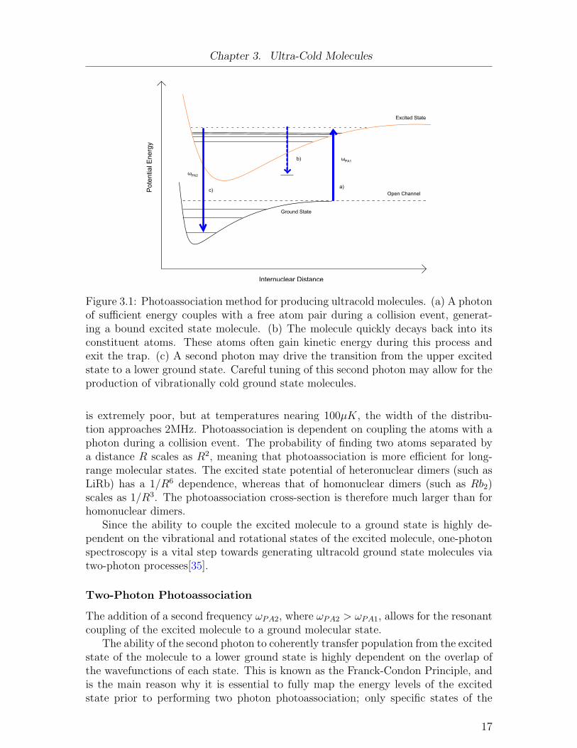
Chapter 3. Ultra-Cold Molecules
Figure 3.1: Photoassociation method for producing ultracold molecules. (a) A photonof sufficient energy couples with a free atom pair during a collision event, generat-ing a bound excited state molecule. (b) The molecule quickly decays back into itsconstituent atoms. These atoms often gain kinetic energy during this process andexit the trap. (c) A second photon may drive the transition from the upper excitedstate to a lower ground state. Careful tuning of this second photon may allow for theproduction of vibrationally cold ground state molecules.
is extremely poor, but at temperatures nearing 100µK, the width of the distribu-tion approaches 2MHz. Photoassociation is dependent on coupling the atoms with aphoton during a collision event. The probability of finding two atoms separated bya distance R scales as R2, meaning that photoassociation is more efficient for long-range molecular states. The excited state potential of heteronuclear dimers (such asLiRb) has a 1/R6 dependence, whereas that of homonuclear dimers (such as Rb2)scales as 1/R3. The photoassociation cross-section is therefore much larger than forhomonuclear dimers.
Since the ability to couple the excited molecule to a ground state is highly de-pendent on the vibrational and rotational states of the excited molecule, one-photonspectroscopy is a vital step towards generating ultracold ground state molecules viatwo-photon processes[35].
Two-Photon Photoassociation
The addition of a second frequency ωPA2, where ωPA2 > ωPA1, allows for the resonantcoupling of the excited molecule to a ground molecular state.
The ability of the second photon to coherently transfer population from the excitedstate of the molecule to a lower ground state is highly dependent on the overlap ofthe wavefunctions of each state. This is known as the Franck-Condon Principle, andis the main reason why it is essential to fully map the energy levels of the excitedstate prior to performing two photon photoassociation; only specific states of the
17

Chapter 3. Ultra-Cold Molecules
excited molecule will couple well with the ground vibrational and rotational state ofthe molecule. By carefully preparing the excited state molecules, and choosing thecorrect wavelength of the second photon, it should be possible to create ultracoldmolecules in the lowest bound energy state[36].
3.2.2 Feshbach Resonance
At ultra-cold temperatures, interatomic collisions are almost entirely s-wave in nature[37].This is due to the low relative velocity of the atom pair, and the small interactionlength. As a consequence, the relevant collision rates of an atomic ensemble aredescribed completely by the s-wave scattering length ao. For instance, the elasticscattering cross section for a pair of bosonic atoms in the ultracold limit is
σ = 8πa2o (3.1)
which further defines the time required for evaporative cooling in a magnetic trap.The s-wave scattering length is essential in the description of cold atomic gas be-haviour; the thermalization rate, mean-field energy, and the stability of the ultracoldatomic cloud are all dependent on this single parameter[38].
Feshbach resonances occur when a quasi-bound state of the system (such as amolecule) becomes degenerate with the collisional energy level of the open free atomchannel. Suppose that at zero magnetic field, the closed channel of the excited molec-ular state is at a higher energy than that of the free atom channel. An asymmetryin the magnetic moments of the two state results in a shift of the relative energy.If the closed channel has a large, negative magnetic moment compared to the openchannel, an increasing magnetic field will result in a decreasing energy difference be-tween the states. This shift in the relative energies is known as ’Zeeman Tuning’. Asthese levels approach degeneracy, the production of molecules from free atoms canbe induced by the coupling of the closed and open channel.
Feshbach resonances provide yet another means of both mapping the interatomicinteraction potential and generating ultracold molecules from a cold atom source.Although homonuclear molecules have been well studied, there exists relatively littleinformation on Feshbach resonances between two different atomic species. Observa-tions of 6Li−23 Na [39] and 40K −87 Rb [40] systems have been made, but only veryrecently have the 6Li −87 Rb resonances that are the focus of our experiment beenobserved[41] .
Pursuing heteronuclear Feshbach resonances, although experimentally and theo-retically more complex than the homonuclear counterpart, gives access to a richerfield of physics. Ultracold heteronuclear molecules provide access to studying Bose-Fermi mixtures with tunable interactions [42], and the possibility of ultracold polarmolecules with extremely high phase-space densities[43].
3.2.3 Electric Field Induced Feshbach Resonances
It has been proposed that collisions between ultracold atoms may be further controlledby use of an external electric field[44]. The theoretical framework for this proposal
18

Chapter 3. Ultra-Cold Molecules
Figure 3.2: Increasing magnetic field strength drives the closed channel closer inenergy to the open channel. A Feshbach resonance occurs for a magnetic field atwhich these two channels become degenerate.
is based on the instantaneous dipole moment formed during the collision of twoatoms. Typical Feshbach resonances couple only the s-wave bound states of the freeatoms, but it has been shown that strong DC electric fields may provide a methodfor coupling initial and final states of differing orbital momenta. This interactionbetween the dipole moment and the electric field is greatly enhanced near p-wavescattering resonances. It is further predicted that the electric-field couplings mayshift the positions of existing Feshbach resonances while possibly inducing new s-wave magnetic resonances in the process.
Experimental Strategy There is progress towards implementing an experimentalsystem to measure these predicted resonances. A pair of DC electrodes have beenfabricated for use within the experimental system. The design was chosen so thatthe electrodes could be positioned within the volume of the trapping cell, close tothe atomic cloud. Machined from 316 stainless steel, the electrodes are supported,
and supplied current, by two extended, 1/4” copper feedthroughs. A Macor© screwis used to adjust the distance between the electrodes while maintaining electricalisolation. Currently, this distance is set to 1.3mm. A photo of the electrodes areshown in fig (3.3).
Since extremely high electric fields are required to probe these new resonances(in excess of 100kV/cm), it is important that the surfaces of the electrodes are assmooth and clean as possible to avoid arcing. After being machined, the electrodeswere polished using successively higher grades of sandpaper, followed by an extensivebuffing stage using a cloth and a commercial metal polisher. There was concern
19

Chapter 3. Ultra-Cold Molecules
that these polishing stages could embed contaminants into the electrodes that couldhinder their functionality, and introduce unwanted materials into the vacuum system.Although this remains a concern, the polishing products were chosen to minimizethese possibilities.
The electrodes were briefly tested in an extra vacuum chamber to check both theplacement and the ability to handle high voltages. The voltage was systematicallyincreased from 0 to 10kV without any sign of arcing or other defects in the build.Asa final means of reducing the surface roughness, the electrodes will be sent out to alocal company to be electropolished.
Figure 3.3: High DC voltage electrodes for use in the electric field induced Feshbachresonance experiment. The electrodes are attached to a 1.33” vacuum CF flangeelectrical feedthrough. Inserted into the vacuum chamber, the extended length willallow the electrodes to be placed physically close to the trapping region of the atomicgas. The spacing of the electrodes is approximately 1.3mm.
Once the electrodes are placed within the second generation experiment, they willbe need to be ‘burned in’ during the vacuum pump out stage. This is accomplishedby slowly increasing the applied voltage in an effort to further clean and smooth thesurface of the electrodes. The small arcing events that occur due to imperfectionsin the electrodes have the advantage of destroying the imperfections in the process.An optical ammeter is in the process of being constructed that would allow for thedetection of these micro-arcs, and allow for the ‘cleaning’ to be done in a controlledmanner.
The electrodes cannot be placed directly at the position of the MOT, so a meansof transporting the trapped atoms from the initial position to one centred withinthe 1.3mm spacing of the electrodes is required. The atoms will first need to betransferred to an optical dipole trap, with the beam of the dipole trap being subse-quently repositioned using two galvos. This will need to be done in a manner thatminimizes trap loss and avoids contaminating the surface of the electrodes. Once thetrapped atoms are positioned, it should be possible to observe losses using absorptionspectroscopy.
20

Chapter 4
Laser Light
Laser light is ubiquitous within this experiment. Cooling, trapping, and manipulat-ing the atoms can all be accomplished through various combinations of wavelengthsand intensities. For this reason there exist a wide range of lasers used within theexperiment, each chosen for specific reasons based on the requirements of the system.
4.1 Requirements
The theoretical framework for laser cooling was based on the assumption of a welldefined two level system, a single wavelength tuned near the transition resonanceis enough to preferentially slow the atoms within the ensemble. In practice thissimplified system is not realized; although we use alkali atoms with only a singleelectron in the outer shell, there exist multiple ground state energy levels for theelectron to decay to. An atom whose electron is lost to the cooling transition is lostto the ensemble. Experimentally it is necessary to incorporate a mechanism thatreintroduces the lost electron back to the cooling transition.
4.1.1 Lithium6Li has the advantage of being a spin-1/2 system. Theoretically this makes it amuch cleaner and simpler model to work with as it is the alkali that most closelyapproximates the electronic structure of hydrogen. Unfortunately, these theoreticalniceties come at the expense of experimental simplicity.
The small mass of lithium results in fine and hyperfine energy level splittings thatare significantly smaller than those for other alkali atoms; specifically a hyperfinesplitting of the ground state of 228MHz, and a splitting of the excited 2P3/2 state(4.4MHz) that is smaller than the natural line-width of the transition (6MHz)[45]. Assuch, Lithium is often approximated as a three level system with two ground stateswith a single excited state transition.
In this three level system, two frequencies of light are required for efficient coolingof Lithium atoms. The first is used to couple the 2S1/2F = 3/2 ground hyperfine stateto the 2P3/2 manifold. This transition is known as the cycling or cooling transition dueto the fast absorption and spontaneous emission rates. The second laser is necessaryto reintroduce atoms that decay to the 2S1/2F = 1/2 state back to the cyclingtransition. The transition to the lower ground state occurs relatively quickly due tothe narrow splitting of the excited state; light tuned near the cycling transition willdrive transitions to all three excited levels. This requires that the repump light forLithium be much more intense than that for Rubidium. Since the atoms scatter light
21

Chapter 4. Laser Light
F=1/2
F=3/2
F’=1/2
F’=3/2
F’=1/2
F’=3/2
F’=5/2
F=1
F=2
F’=1
F’=2
F’=3
F’=2
F’=1
F’=0
2 2S1/2
2 2P1/2
2 2P3/2
2 2S1/2
2 2P1/2
2 2P3/2
6Li 7Li
2.88 MHz
152.14 MHz
10.053 GHz
10.052 GHz
18 MHz
92 MHz
804 MHz
670.776 nm
670.776 nm
D1 line
D2 line
D1 line
D2 line
76.07 MHz
8.69 MHz
17.37 MHz
1.17 MHz
1.74 MHz
10.53 GHz
COOLING
RE-PUMP
Figure 4.1: Energy level diagram of 6Li with 7Li shown for comparison. The coolingand repump light transitions are shown. [1]
nearly as often from the repump beams, they must be made to contribute to the lasercooling and so are integrated into the system along all six directions with the coolinglight. Further, the unresolved nature of the excited hyperfine states severely limitsthe efficiency of sub-Doppler cooling. The polarization gradient is contingent on awell defined ‘closed’ transition that is not available for Lithium atoms.
An acousto-optic modulator, discussed further in the Control System Hard-ware section, can be used to induce a frequency shift of the master laser output inorder to produce light for both the cooling and repump transitions.
4.1.2 Rubidium
Rubidium requires a separate master laser for both the cooling and repump light asthe ground state hyperfine splittings are many gigahertz apart. Further, the excitedstate cannot be approximated as a single level as is the case for Lithium. The resultis that the decay rate from the cooling transition is much lower; repump light of lowpower along a single direction of the MOT beams is sufficient for repopulation to thecooling states.
22

Chapter 4. Laser Light
F=1
F=2
F’=2
F’=1
F’=0
5 2S1/2
5 2P3/2
87Rb 85Rb
72.22 MHz
4.271 GHz
780.241 nm
D2 line
2.563 GHz
193.7 MHz
156.9 MHz
COOLING
RE-PUMP
72.91 MHz
F’=3
F=2
F=3
F’=3
F’=2
F’=1
5 2S1/2
5 2P3/2
113.2 MHz
1.771 GHz
780.241 nm
D2 line
1.265 GHz
100.3 MHz
83.87 MHz
COOLING
RE-PUMP
20.49 MHz
F’=4
Figure 4.2: Energy level diagrams for 85Rb and 87Rb with the corresponding coolingand repump transitions shown.[1]
4.2 Master and Slave Lasers
There exist commercially available semiconductor lasers with natural output wave-lengths close to the transition wavelengths of 780nm for 85,87Rb and 671nm for 6Li.These diode lasers produce light through the application of a forward bias currentacross a p-n junction, stimulating the recombination of electrons and holes[10].
Ultra-stable, well-collimated reference light is generated by locking the output ofsingle ‘master’ laser to a specific energy transition of the atom by way of a saturatedabsorption spectroscopy technique[46]. This is a well established technique, describedlater, that provides a wide tunability with a narrow bandwidth. Amplification of thisreference light is achieved through injection locking of further diode lasers.
In all, five master lasers are necessary for the experiment. Four are required for85,87Rb and one for 6Li. The light from each of the Rubidium masters is sent to a slavelaser for amplification. Most of the amplified light is then coupled into an opticalfiber and sent to various experiments, with a small amount of light being reserved fordiagnostic use by way of a Fabry-Perot interferometer. The interferometer is integralfor verifying that the slave lasers are adequately locked to the appropriate frequency.The Lithium light is similar, except that the light is first frequency shifted using
23

Chapter 4. Laser Light
an acousto-optical modulator such that the correct frequencies for the cooling andrepump light (spaced 228MHz apart) are achieved. These distinct frequencies arethen amplified and sent out to various experiments.
4.2.1 Master Locking Technique
Semiconductor diode lasers suffer from two major drawbacks; the output power of asingle diode is a fraction of the total power needed for the experiment, and the naturallinewidth of the emitted light spans hundreds of megahertz. Fortunately, the latterissue can be corrected through feedback mechanisms, while the former is compensatedfor through the introduction of an amplification system based on an injection schemefor diode lasers that remains extremely cost effective when compared with other lasersystems[47].
The diode laser consists of a semiconductor gain medium enclosed within a res-onator cavity. The short diode laser cavity is typically on the order of a millimetrewith a low front facet reflectivity, and a broad frequency linewidth of the emitted light( 100MHz). A diffraction grating, placed external to the diode cavity and driven bypiezoactuators, is used to narrow and stabilize the output frequency of the laser[48].The first order diffracted beam is reflected back into the laser cavity, This injectedlight results in a saturation of the gain medium and the extinction of all other com-peting frequencies. This is known as a Littrow configuration[49]. The frequency ofthe light is then controlled by changing both the angle of the diffraction grating,and the length of the resonator cavity by means of current and temperature. Thefrequency is narrow and stabilized only when the injected light couples resonantlyinto the diode cavity[50].
Figure 4.3: Schematic representation of the Littrow configuration used as a feedbackmechanism for the master laser diodes. The grating and mirror are monolithic andmove as a single entity in order to minimize the translation of the output beam asthe grating angle and cavity are varied.
Saturated absorption spectroscopy is used to determine the exact location of theenergy transition. From the output of the master laser, a fraction of the light pickedoff, split using a PBS, and sent as counterpropagating beams along the ±z axis of
24

Chapter 4. Laser Light
either a Rubidium vapour cell or a Lithium heat pipe (the vapour pressure of Lithiumdoes not allow for a room temperature vapour cell). Referred to as the pump andprobe beams, they have identical frequencies ν0 but opposite k vectors. The probebeam is detected on a photodiode; in the absence of any pump beam, the absorptionsignal will follow a frequency dependent Voigt profile due to the convolution of thenatural Lorentzian line shape and the Maxwell-Boltzmann distribution of the atomvelocities within the vapour cell. The addition of the higher intensity, counter prop-agating pump beam results in the appearance of sharp dips in the absorption profileat frequencies corresponding to resonances of the vz = 0 atoms.
In order to generate an error signal for locking purposes, the light of the pumpbeam is frequency modulated by some small amount δv such that the new frequencyis given by v = vo + δv sin(ωt). This is achieved with an acousto-optical modulatordriven by a sinusoidally varying frequency signal from a direct digital synthesizer(DDS, described further within the QDG control system section). The intensityof the saturated absorption signal detected on the photodiode is dependent on thefrequency of the pump and probe beams. The frequency modulated intensity of thephotodiode signal, when expanded about the initial frequency ν0, is given by
I(v) = I(vo) +dI
dv|vo(δv sin(ωt)) +
1
2
d2I
dv2|vo(δv sin(ωt))2 +O(δv)3 (4.1)
A home-built electronic ‘lock-box’ is used to produce a feedback signal[51]. Thelock box consists of a lock-in amplifier and a PI controller. The modulated satu-rated absorption signal is multiplied with a sine wave of the modulation frequency(177.8kHz) and time averaged to extract the error signal (∂I
∂v). Adjusting the phase
difference ∆φ between the absorption signal and the reference frequency allows forthe maximization of the output signal.
OutputAmplitude =1
T
∫ T
0I(v, ω) · sin(ωt+ φ) ∝ dI
dv|voδv (4.2)
The derivative of the absorption signal is used as the error signal for a feedbackcontroller. The derivative of a saturation dip in the Voigt profile of the absorptionsignal is shown in fig (4.4). Locking to the zero crossing of this signal by use of astandard proportional-integral stage feedback loop allows for frequency stabilizationof a few MHz. A slow correction output to the PZT voltage compensates for acousticfluctuations of the grating position and for temperature drifts by adjusting the angleof the grating and the cavity length of the external laser cavity, while a fast correc-tion output to the current controller compensates for small and fast fluctuations byadjusting the injection current to the diode.
4.2.2 Injection Locking of Slave Lasers
As discussed, the output from a single master laser is insufficient for the experiment.Light from the master laser is coupled into the gain medium of the slave laser diode.If the frequency of the master light is resonant with the internal cavity of the diode,then this frequency will saturate the gain medium and extinguish competing modesso that the slave laser output is pulled to a single, well-defined frequency at its natural
25

Chapter 4. Laser Light
Figure 4.4: Sample error signal (shown in black) derived from the saturated absorp-tion spectrum (shown in blue) for 6Li. The laser frequency is locked to the zerocrossing of the error signal.
output power. The master light is coupled into the output path of the slave laserthrough the side port of an optical isolator. The temperature and current of the slavelaser are critical in ensuring that the master light is amplified. If these values are notset correctly, the output of the slave laser will not follow the injected master light.
4.3 Photoassociation Laser
The photoassociation laser is a Coherent Ti:Sapphire 899-21 pumped by a 10W Co-herent Verdi laser. Since our interest is in the study of the molecular potentialscorresponding to the asymptotic atomic states Li + Rb∗, the laser will be scannedfrom a wavelength of 795nm, corresponding roughly to the D1 and D2 transitions ofRb∗, and continuing further to the red.
The laser is locked to a frequency comb of a mode locked fiber. This should reducethe linewidth of the Ti:Sapphire laser to the kHz range. Scanning the wavelength ofthe laser is accomplished by tuning the repetition rate of the fiber comb.
The photoassociation light will be coupled into the trapping cell along the sameoptical axis as the dipole trap light. This is done due to space constraints, and toallow the greatest overlap between the trapped atoms and the photoassociation light.
26
Chapter 4. Laser Light
4.4 Fiber Laser for Optical Dipole Trap
As discussed in the preceding theory section, atoms can be trapped by exploiting theinteraction between an induced atomic dipole and a radiation field. A high intensity,strongly focused laser beam will have an attractive potential if the wavelength istuned to the red of an atomic transition.
In order that the light is not resonant with any atomic transition, and in orderthat the scattering rate is as small as possible to avoid heating, it is advantageousthat the wavelength should be detuned as far to the red as possible. Since the trapdepth is inversely proportional to the detuning, a high intensity field is needed ascompensation. Currently, a 20W fiber laser from IPG outputting a single-mode,linearly polarized beam at a wavelength of 1064nm is being used as the source forthe dipole trap.
Theoretical calculations [2] show that the potential energy difference between theopen channel and the first excited state of the LiRb molecule to be at 2182.1nm.It is therefore possible that the wavelength of the laser may result in the excitationof ground state molecules. The linewidth of such a transition, contingent on itsexistence, should be smaller than that of the bare atomic states (6MHz) due to theFranck-Condon overlap between the free and deeply bound states. Although this isa limiting factor, it could be overcome by simply tuning the narrow band trappinglaser away from such a resonance.
An optical trap is based on the dipole force, described earlier, and is highly de-pendent on the intensity of the light. Since there does not exist a saturation intensity,as is the case for Doppler cooling, it is beneficial to increase the intensity of the lightas much as possible. Initially, the dipole trap will consist of light from the 1064nmfiber laser focused to a 50µm waist close to the MOT. The light will be reflected backthrough the cell in order to increase the trap depth by way of an increased intensity.Future iterations of the dipole trap will use a stabilized resonator cavity to approachintensities of 120W.
4.5 Ionization Laser
An ionization laser is necessary to perform time of flight measurements of the molec-ular ions. Initially, an Nd:YAG Continuum Minilite, frequency doubled to 532nm,was to be used as the ionization laser within this experiment. The laser emits 5.6nspulses at peak energies of 25mJ per pulse. The time of flight apparatus was devel-oped and implemented by Nina Rauhut as part of her diplome work [2]. Although theapparatus has been successfully placed within the first generation experiment, it iscurrently inoperable due to technical reasons. The ionization laser was on loan fromanother research group, and recently needed to be returned. Possible replacementsfor this light source are being discussed, but as it is not currently required for thefirst generation experiment the final purchase will be delayed until later. Before thelaser was returned, it was used to test the viability of laser ablation as a means ofloading a Lithium MOT without the use of an emissive oven. These results of thistest will be presented later within the Measurements chapter.
27

Chapter 5
Experimental Setup
A dual species Li and Rb MOT is necessary for the production of heteronuclear polarmolecules. As was discovered, working with these laser cooled gases requires a widerange of expertise; including working knowledge of vacuum systems, atomic sources,and detection methods.
5.1 Vacuum System
Ensembles of cold atoms are delicate and can only be produced in an ultra highvacuum (UHV) environment. UHV is typically characterized by pressures below10−9 torr.
Creating a UHV is a difficult prospect, creating one with the added restrictionsplaced on the system by the experiment requires careful planning and handling duringall steps of the process. Nitrile gloves are worn when handling any of the vacuumsystem, the natural oils from a fingerprint are enough to keep the vacuum fromreaching the necessary limit. The parts used must be composed of materials with verylow vapour pressures — if even one component within the vacuum does not conform tothis standard, then natural outgassing occurring from the materials may be too highto maintain a suitably low pressure within the vacuum chamber. Finally, any materialat room temperature will naturally have organics, as well as air and water adsorbedto the surface. If left in this state, these components will slowly degas within thevacuum chamber and cause the background pressure to rise. To counter this, all partsare cleaned thoroughly in a series of ultrasonic baths consisting of a degreasing agent,clean water, methanol, and finally finished with acetone. The parts are assembledquickly to avoid recontamination, then heated to a temperature between 200 C and450 C while the chamber is being pumped(certain parts, especially those with aglass to metal transition, cannot be heated as high as parts that are all metal. Ingeneral the assembly is heated to the highest temperature possible for all parts). Thisaccelerates the outgassing of the materials and the degassing of the adsorbed air andwater so that when the assembly is cooled a much lower pressure is attainable. Thisbaking procedure can extend upwards of weeks, and can consist of multiple cycles inorder to achieve the lowest possible background pressure.
5.1.1 Trapping Cell
The trapping cell is the most important part of the vacuum system. Our cell is com-posed entirely of highly polished, optical quality Borosilicate glass in order to allowfor a greater range of optical access for the numerous light beams and detection de-vices. Purchased from OptoSigma, the cell is 9.5cm in length with an inner diameter
28
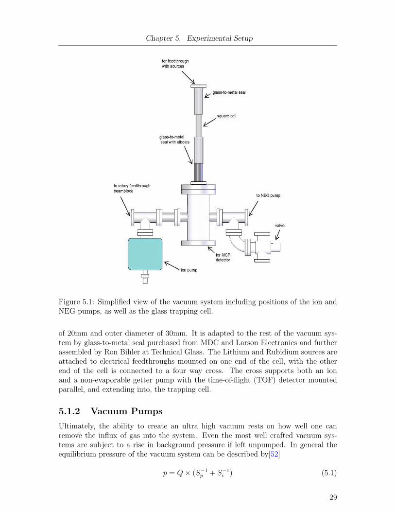
Chapter 5. Experimental Setup
Figure 5.1: Simplified view of the vacuum system including positions of the ion andNEG pumps, as well as the glass trapping cell.
of 20mm and outer diameter of 30mm. It is adapted to the rest of the vacuum sys-tem by glass-to-metal seal purchased from MDC and Larson Electronics and furtherassembled by Ron Bihler at Technical Glass. The Lithium and Rubidium sources areattached to electrical feedthroughs mounted on one end of the cell, with the otherend of the cell is connected to a four way cross. The cross supports both an ionand a non-evaporable getter pump with the time-of-flight (TOF) detector mountedparallel, and extending into, the trapping cell.
5.1.2 Vacuum Pumps
Ultimately, the ability to create an ultra high vacuum rests on how well one canremove the influx of gas into the system. Even the most well crafted vacuum sys-tems are subject to a rise in background pressure if left unpumped. In general theequilibrium pressure of the vacuum system can be described by[52]
p = Q× (S−1p + S−1
i ) (5.1)
29

Chapter 5. Experimental Setup
where Q represents the total influx of gas into the system from outgassing, de-gassing, leaks, and connections to other systems at a different pressures. Sp repre-sents the speed of the pump in liters/second, and Si represents the throughput ofthe connections between the vacuum system and the pump. Generally for atom trapexperiments the volume of the vacuum is kept relatively small, typically less than 10litres. With such small volumes, pumps designed for commercial applications (higherpressures but much larger volumes) are more than adequate in achieving UHV. Thelimiting factor in obtaining a really good UHV is almost entirely concentrated inmaximizing the throughput of the connections between the pump and the vacuum.
Unfortunately, there does not exist a single pump capable of pumping efficientlyover the entire range of pressures or the full range of elements required to obtainUHV[53]. For this reason it is necessary to use a combination of pumps, each onedesigned for use in a specific pressure regime and best suited to removing certaintypes of elements found within the vacuum. A turbo pump is used to quickly reducethe pressure from atmosphere to 10−4 torr, this pump is most useful during periodsof baking and is removed by way of a bakeable valve when the vacuum system ismounted within the experiment. Lower pressures are achieved and maintained by acombination of an ion pump and a non-evaporable getter (NEG) pump. These pumpsremain connected and active during the entire lifetime of the experiment.
Turbo Molecular Pump
Turbo molecular pumps were first introduced in 1957 [54] and work on the principlethat particles can be accelerated in a specific direction using repeated collisions witha solid, moving surface. A high speed turbine rotor, whose blades have been angledin order to maximize the momentum transfer, is used to preferentially pump outgas molecules that collide with the blades. Used widely in industry and research forachieving moderately high vacuums, they are capable of pumping 70 litres/secondwith rotor speeds of 80,000 rev/min.
A Varian V70 turbo molecular pump was used in the bake-out of the vacuumchamber when large pumping speeds are integral in removing the high influx of de-gassed particles.
Ion Pump
Ion pumps become useful when the pressure drops below 10−5 torr and are used onlyafter the turbo pump has reduced the background pressure to an acceptable level. Ionpumps consist of multiple anode cells with usually two cathodes. Ions are formed fromthe gas molecules present in the vacuum system by way of electrostatic discharge.The strong electric field of the discharge then accelerates the ionized particle towardthe cathode where it is either buried directly, or reflected to be buried in anothercontainer. The magnet produces cyclotron motion of the free electrons, improvingthe ionization of the gas to be pumped. Further, the pump also works by bindingreactive gases to a metal such as titanium. In both instances, particles are notremoved from the system but instead are bound either chemically or physically so asto no longer contribute to the pressure of the system.
30

Chapter 5. Experimental Setup
Due to the strong magnetic fields present, ion pumps must usually be placed at adistance from the main experiment. This constraint tends to reduce the throughputof the system. Ion pumps are also inefficient with respect to particles of low reac-tivity and many hydrocarbons. A Varian StarCell pump, capable of pumping at 20litres/second, is used in our experiment.
Non-Evaporable Getter Pump
Non-evaporable getter pumps contain a highly reactive getter material that adsorbsactive gas molecules through chemical reactions. The pump is activated by resistivelyheating the getter material, diffusing the passive surface layer into the bulk. Devoidof magnetic fields, or vibration inducing moving components, the pump can be placedarbitrarily close to the experimental chamber. Our experiment uses an SAES Ca-paciTorr pump using both a Ti-V alloy and a sintered Zr-V-Fe alloy as the reactivegetter material. NEG pumps are very efficient in removing water and hydrogen, twomajor contaminants in vacuum systems.
5.2 Atomic Sources
5.2.1 Rubidium
Rubidium is selectively released using a commercial SAES Getters dispenser contain-ing Rb2CrO4 and ZrAl in a stainless steel container. The ZrAl acts as a reducingagent and is responsible for not only returning the Rubidium alloy to its pure metal-lic state, but also for absorbing chemically reactive gases present in the dispenser.Passing a current through the dispenser results in the emission of atomic 85Rb and87Rb vapour at their natural abundances of 72.17% and 27.83%.
5.2.2 Lithium
Lithium isotopes exist naturally in both fermionic (6Li) and bosonic (7Li) forms. Forthe purpose of this experiment, only the fermionic form is of interest; the bosonicform is essentially an unwanted impurity. This presented two major obstacles; thenatural abundance of 6Li is only 7.5%, and the low vapour pressure of lithium atroom temperature meant that building a dispenser was not a viable option. The firstissue was resolved by using an enriched source of 6Li (95%), reducing greatly thecontamination from 7Li. The second issue necessitated building an effusive atomicbeam source. The source consisted of an 80mm3 reservoir machined from NiCr witha small exit hole. Resistive heating of a small 6Li enriched crystal resulted in evap-oration; the small exit hole of the oven confined the output to a collimated atomicbeam source.
Typically an atomic source of this nature is implemented with a Zeeman slowerin order to access a much larger section of the velocity distribution of the atoms[55].Technical complexity and space considerations led to discussions concerning the ben-efits of a slowing system for use within our experiment. Naturally, eliminating any
31

Chapter 5. Experimental Setup
Figure 5.2: Direct view of the atomic sources used within the experiment. Attached toa UHV feedthrough, the Rb atoms are dispensed by way of a temperature dependentchemical reaction while the Li atoms are emitted from the effusive oven as the metalis heated above its melting point.
slowing mechanisms means that the number of atoms that our cooling light will haveaccess to will be severely limited. However, this is compensated for slightly by be-ing able to move the Lithium oven much closer to the position of the MOT, and byreducing the total volume of the vacuum system. The first increases the number ofatoms that reach the trapping region, while the second allows for a smaller back-ground pressure. A simple mechanical beam block is used to shelter the trappingregion from being directly bombarded by hot Lithium atoms. Since we are mainlyconcerned with loading the cooled atoms into an optical dipole trap, where 105 atomsare sufficient for our experiments, we don’t require large atom numbers in the MOTto begin with. For a more complete analysis of the motivation behind this methodsee S. Singh’s Master’s Thesis[1]. Initial measurements of the Li MOT are presentedwithin the Measurements section.
5.3 Helmholtz and Compensation Coils
Magnetic fields are required for numerous aspects of the experiment. They are re-quired to compensate for the earth’s magnetic field, for use in a magneto-optical trap,for use in a pure magnetic trap, and, finally, for creating Feshbach resonance fields.
32

Chapter 5. Experimental Setup
5.3.1 Compensation Coils
The compensation system consists of three pairs of coils in an anti-Helmholtz con-figuration. Each coil is composed of eighty windings of Kapton coated copper wires.They are placed so that each pair is perpendicular to one of the axes of the MOTlight. The current through each coil is independent of the others; full control of thezero of the field is possible. These coils are used primarily to offset the earth’s mag-netic field, but can also be used to change the position of the MOT within the trapcell.
5.3.2 Helmholtz Coils
The Helmholtz coils are used to produce fields for everything else. Two identicalcoils are placed in the z-axis and are separated by a distance equal to the radiusof the coils. Current can either be sent through the coils in the same direction, orin opposite directs. For current travelling in the same direction, the magnetic fieldproduced is spatially uniform in a cylindrical region extending between the center ofthe coils. The field produced is calculated to be [56]
Bz = µoIR2
(D2 +R2)3/2+ µoI
3R2 (4D2 −R2)
2 (D2 +R2)7/2
(z2 − ρ2/2
)+ ... (5.2)
Bρ = µoI3R2 (4D2 −R2)
2 (D2 +R2)7/2zρ+ ... (5.3)
where z is the position along the axis, Bz is the magnetic field component alongthat axis, ρ the radial position, Bρ the radial field component, µo the permeabilityconstant, I the current, R the radius of the loop, and 2D the separation. For aHelmholtz configuration, where R = 2D, the fields reduce to
Bz = µoI8
5√
5R+ ... (5.4)
Bρ = 0 + ... (5.5)
From this it can be seen that the radial component is zero, while the componentalong the z-axis is uniform. This configuration is used for creating the large, uniformmagnetic fields necessary for Feshbach resonance studies.
For currents running in opposite directions, the fields are given by
Bz = 3µoIDR2
(D2 +R2)5/2z +
15
24µoI
R2 (4D2 − 3R2)
(D2 +R2)9/2
(4z3 − 6ρ2z
)+ ... (5.6)
Bρ = −3
2µoI
DR2
(D2 +R2)5/2ρ+
15
16µoI
R2 (4D2 − 3R2)
(D2 +R2)9/2
(ρ3 − 4ρz2
)+ ... (5.7)
In this case, the third order terms do not vanish for R = 2D as in the Helmholtzconfiguration. Instead, to first order, the gradient fields are maximized
33

Chapter 5. Experimental Setup
dBz
dz= µoI
48
25√
5R2= 2
dBρ
dρ(5.8)
This is important for use as the magnetic field for a MOT. The anti-Helmholtzconfiguration gives a linear (to first order) field in both ρ and z with a maximizedgradient.
Each coil, constructed by Paul Lebel [57], consists of approximately 250 windingsof Kapton coated copper wire housed in a watertight PVC chamber. The contributionfrom these loops, for a maximum current of 25A, is predicted to be near 1kG. Thesecoils are water cooled as the power dissipation when run at maximum field gradientsis close to 1kW.
A coil driver, constructed by the UBC electronics lab, is used to toggle the coilsbetween a Helmholtz or anti-Helmholtz configuration. The driver is controlled witha digital input for quickly switching the current on and off, and an analog input forcontrolling the current supplied to the coils. Toggling the coils from a Helmholtz toanti-Helmholtz configuration must be done manually by reversing the polarity of theoutput ports of the coil driver. In this way a single pair coils can be used in both thepreparation of the trapped atom cloud and also later for use in feshbach resonancestudies. When used for trapping, the typical current to the coils is between 4 and6A.
5.4 Photoassociation Table
The master light is transported via fiber optical cables to a separate optical tablewhere the vacuum chamber and MOT cell are housed. Once the light arrives at thetable, it is necessary to further amplify and condition the light for use within theexperiment.
The Lithium light arrives to the Photoassociation table already possessing theproper frequencies needed for the experiment. Both the cooling and repump light areamplified through the use of slave lasers. The Rubidium cooling light is amplifiedusing a single slave laser. The amplified light is then sent through an AOM doublepass configuration in order to shift the light to the proper frequency. The Rubidiumrepump light does not require any amplification, but a further frequency shift usingan AOM double pass is necessary. The frequency of the light is further shifted on thePhotoassociation table for a few reasons; the light is shared among many experimentsand this method allows for all of them to be independently functional, and it greatlysimplifies the experimental sequencing of devices by keeping any necessary changeslocal to the Photoassociation table.
The Rubidium repump light only needs to be coupled into the MOT along asingle axis. Since the optical pumping is much stronger for Lithium, the repumplight needs to be coupled along all three axis with the cooling light for Rubidium andLithium. To this end, both frequencies of Lithium light are combined on a polarizingbeam splitter (PBS) with the Rubidium cooling light combined with the Lithiumfrequencies using a dichroic mirror coated to reflect the Rubidium light but transmitthe Lithium light. Initially a PBS was used in lieu of the dichroic mirror, but issues
34
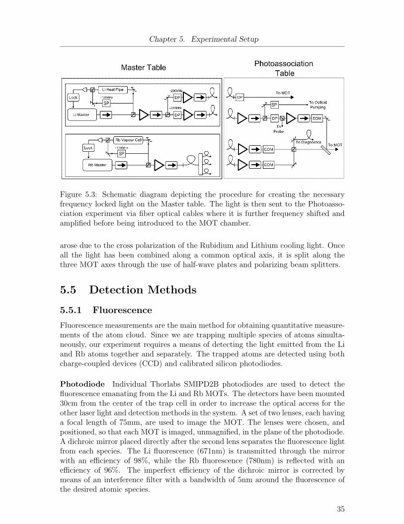
Chapter 5. Experimental Setup
Figure 5.3: Schematic diagram depicting the procedure for creating the necessaryfrequency locked light on the Master table. The light is then sent to the Photoasso-ciation experiment via fiber optical cables where it is further frequency shifted andamplified before being introduced to the MOT chamber.
arose due to the cross polarization of the Rubidium and Lithium cooling light. Onceall the light has been combined along a common optical axis, it is split along thethree MOT axes through the use of half-wave plates and polarizing beam splitters.
5.5 Detection Methods
5.5.1 Fluorescence
Fluorescence measurements are the main method for obtaining quantitative measure-ments of the atom cloud. Since we are trapping multiple species of atoms simulta-neously, our experiment requires a means of detecting the light emitted from the Liand Rb atoms together and separately. The trapped atoms are detected using bothcharge-coupled devices (CCD) and calibrated silicon photodiodes.
Photodiode Individual Thorlabs SMIPD2B photodiodes are used to detect thefluorescence emanating from the Li and Rb MOTs. The detectors have been mounted30cm from the center of the trap cell in order to increase the optical access for theother laser light and detection methods in the system. A set of two lenses, each havinga focal length of 75mm, are used to image the MOT. The lenses were chosen, andpositioned, so that each MOT is imaged, unmagnified, in the plane of the photodiode.A dichroic mirror placed directly after the second lens separates the fluorescence lightfrom each species. The Li fluorescence (671nm) is transmitted through the mirrorwith an efficiency of 98%, while the Rb fluorescence (780nm) is reflected with anefficiency of 96%. The imperfect efficiency of the dichroic mirror is corrected bymeans of an interference filter with a bandwidth of 5nm around the fluorescence ofthe desired atomic species.
35

Chapter 5. Experimental Setup
Figure 5.4: The photodiode fluorescence imaging system. The light for both atomicspecies is imaged independently on PD1 and PD2 through the use of a dichroic mirrorand two interference filters (IF1 and IF2).[2]
The signal from the photodiode can be related directly to the number of trappedatoms by the following expression;
Pdet =hcΩ
4πλ· L ·R ·Natoms · Γscatt (5.9)
where hcλ
is the energy of a single photon, Ω4π
is the solid angle subtended by thedetection system at the atomic cloud, L is the signal loss due to optical components,andR is the responsivity of the photodiode in millivolts. This will be further discussedin the Measurements section.
Camera A Pixelink PL-A714 monochrome camera with a 1280 × 1024 resolutionand a variable frame rate is used to detect fluorescence due to spontaneous photonemission after a scattering event. It is controlled externally through class functionswritten into the QDG control system software. In this way, images can be coordinatedwith state changes in the system.
5.5.2 Absorption
This method images the shadow cast by the atomic cloud on a resonant probe beam.Since the laser light is sent through the region of the cloud, it is important that thewidth of the light beam is larger than the dimension of the region to be imaged. Afterthe beam has passed through the atomic cloud, it is imaged onto a CCD camera sothat the plane of the MOT is in focus. An Apogee Alta series U6 camera, as well asthe Pixelink camera described above are used to for this measurement.
5.6 RF State Selection
As discussed in the evaporative cooling section, a magnetic field produces a split inthe hyperfine levels of the atom that is dependent on the radial distance from thefield minimum. Control of the atomic state is an important part of the experiment
36
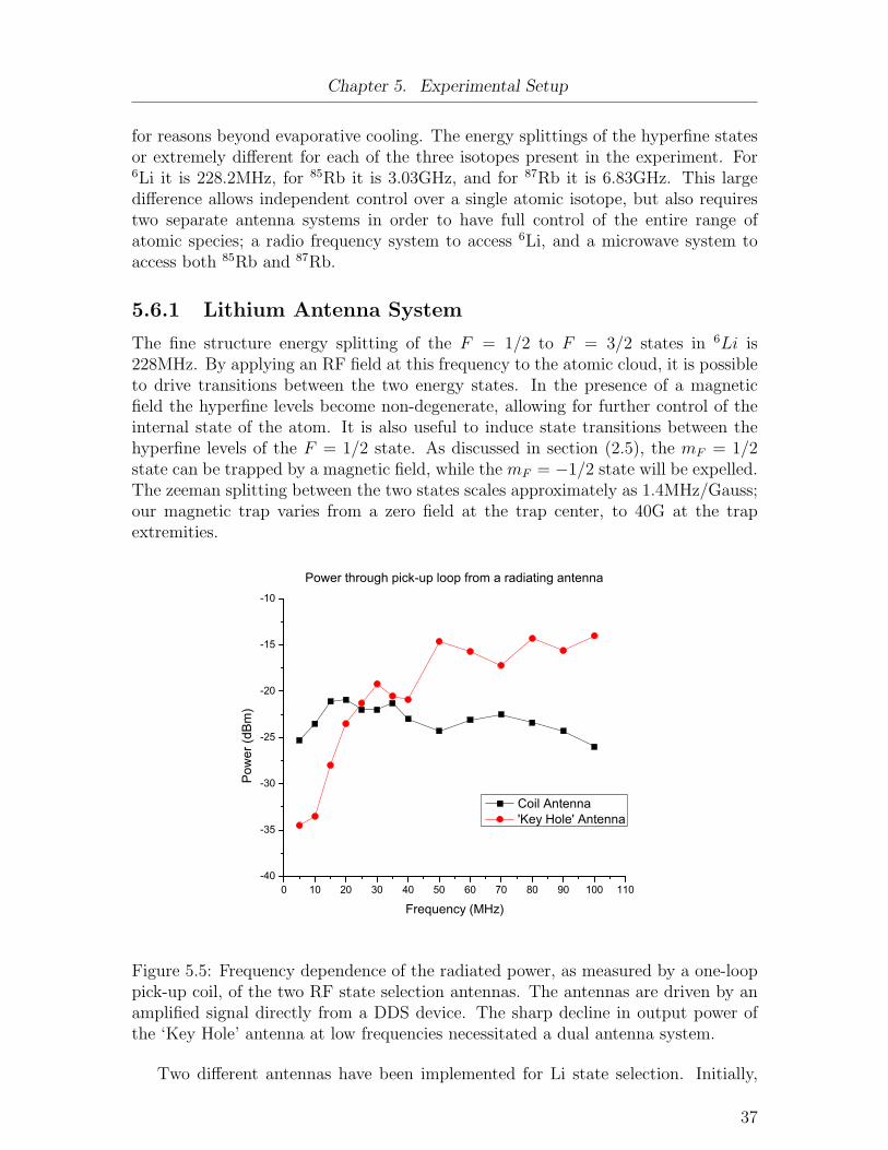
Chapter 5. Experimental Setup
for reasons beyond evaporative cooling. The energy splittings of the hyperfine statesor extremely different for each of the three isotopes present in the experiment. For6Li it is 228.2MHz, for 85Rb it is 3.03GHz, and for 87Rb it is 6.83GHz. This largedifference allows independent control over a single atomic isotope, but also requirestwo separate antenna systems in order to have full control of the entire range ofatomic species; a radio frequency system to access 6Li, and a microwave system toaccess both 85Rb and 87Rb.
5.6.1 Lithium Antenna System
The fine structure energy splitting of the F = 1/2 to F = 3/2 states in 6Li is228MHz. By applying an RF field at this frequency to the atomic cloud, it is possibleto drive transitions between the two energy states. In the presence of a magneticfield the hyperfine levels become non-degenerate, allowing for further control of theinternal state of the atom. It is also useful to induce state transitions between thehyperfine levels of the F = 1/2 state. As discussed in section (2.5), the mF = 1/2state can be trapped by a magnetic field, while the mF = −1/2 state will be expelled.The zeeman splitting between the two states scales approximately as 1.4MHz/Gauss;our magnetic trap varies from a zero field at the trap center, to 40G at the trapextremities.
0 10 20 30 40 50 60 70 80 90 100 110-40
-35
-30
-25
-20
-15
-10
Pow
er (d
Bm
)
Frequency (MHz)
Coil Antenna 'Key Hole' Antenna
Power through pick-up loop from a radiating antenna
Figure 5.5: Frequency dependence of the radiated power, as measured by a one-looppick-up coil, of the two RF state selection antennas. The antennas are driven by anamplified signal directly from a DDS device. The sharp decline in output power ofthe ‘Key Hole’ antenna at low frequencies necessitated a dual antenna system.
Two different antennas have been implemented for Li state selection. Initially,
37

Chapter 5. Experimental Setup
a ‘Key Hole’ antenna was developed for use at 228MHz. This design was primarilymotivated by anecdotal advice on the radiative properties of certain antenna designs.It is important that the RF signal couple well into the antenna so as to minimizepower loss, and it was advised that this design had been seen to be the most efficientwithin similar frequency ranges. The first iteration consisted of two antennas placedin a Helmholtz configuration to maximize the radiation power at the position of theatomic cloud. Although marginally more efficient than a single antenna design, spaceconstraints within the experimental setup made the dual antenna setup unfeasible.
The ‘Key Hole’ antenna was first tested in situ by scanning the frequency fromDC to 40MHz in an attempt to empty a magnetic trap of Li atoms. Proving un-successful, a ten coil loop antenna, with a diameter equal to that of the ‘Key Hole’design, was quickly built and tested in a similar manner. With this design provingcapable of emptying the magnetic trap of atoms, it was necessary to characterizeboth implementations in order to discern the possible reasons for the initial failure.
60 80 100 120 140 160 180 200 220 240 260
-40
-35
-30
-25
-20
-15
-10
-5
Pow
er (d
Bm
)
Frequency (MHz)
Coil Antenna 'Key Hole' Antenna
Power through Pick-up Loop from a Radiating Antenna
Figure 5.6: Determination of the radiated power of the dual antenna system at highfrequencies measured by a one-loop pick-up coil on axis at a distance R from thecenter of the coils. The antennas are driven by an amplified, frequency doubled DDSsignal.
Figs. (5.5) and (5.6) show the relative power fluctuations through a small pick-upcoil placed at the equivalent position of the atomic cloud. As predicted, the ‘Key Hole’design is much more efficient across most of the relevant frequencies, except within asmall region extending from DC to approximately 25MHz where the efficiency of the‘Key Hole’ antenna degrades rapidly. Since this range is critical in manipulating thestate transfer between the ground hyperfine states, it was decided that a dual system
38

Chapter 5. Experimental Setup
would be implemented; one using a simple ten coil loop antenna driven directly byan amplified DDS signal, and the second using the ‘Key Hole’ antenna driven by a228MHz amplified signal derived from a frequency doubled 114MHz DDS output.
Figure 5.7: Schematic diagram showing the dual antenna implementation for RFstate selection. The coil antenna is used to drive hyperfine ground state transitionsbelow 40MHz, while the ‘Key Hole’ antenna is used to drive transitions at 228MHz.
A schematic diagram showing the method used for controlling the RF signal andcoupling it into the atomic cloud is shown in Fig (5.7). In each system, a DDS unitis used to generate the continuous wave RF radiation. The output frequency andamplitude are fully controlled from within the QDG Control System.
Rubidium Antenna System The Rubidium antenna system is being developedto supply microwave frequencies at 3.0 and 6.4GHz to trapped samples of 85,87Rbgas. These frequencies correspond to the fine level splitting in the Rubidium isotopes(Fig. (4.2)). Currently, the components necessary for the signal generation have beenbuilt or purchased but are not fully integrated. As the components are modular,the difficulty is only in ensuring that the feedback locking system for the voltagecontrolled oscillator (VCO) output is working. A major aspect of the design, andone that hasn’t been fully formalized, is that of the microwave antenna needed tocouple the generated signal into the volume occupied by the Rb MOT. As was thecase with the Lithium antenna, this will most likely require multiple design trialswith empirical data to determine the efficiency.
39

Chapter 5. Experimental Setup
Figure 5.8: Schematic diagram showing the signal generation of the microwave stateselection system. A single voltage controlled oscillator (VCO) is used to produce thenecessary frequencies for both Rb isotopes. The implementation of an antenna tocouple these fields has yet to be realized.
40

Chapter 6
Control System Hardware
The QDG control system has had many implementations and developers since itsearly inception. Much of the hardware is based on modified versions of Todd Meyrath’sand Florian Schreck’s designs while at the University of Texas at Austin. It is fromhere that the UTBus standard was devised, and where electronic designs of devicesnot directly associated with the control aspect of the experiment were first imagined.
6.1 Motivation
The nature of cold molecule experiments require precise control of both the statechange of individual components, as well as the timing of these events. This con-trol must be highly configurable and infinitely repeatable; the system must be flexibleenough to accommodate the future addition of modular components, but rigid enoughto repeat the same experiment continuously in order to accumulate the necessary datafor proper statistical analysis. What follows is a detailed description of the implemen-tation of the QDG computer control system; the hardware setup,the impetus behindthe software design, the current state of the software, and the things that still needto be put in place.
6.2 Hardware Components
The hardware components of the QDG control system can be separated hierarchicallyby their functionality within the experimental system and by how they are accessedduring an experimental sequence.
6.2.1 The UTBus
The UTBus is a parallel, uni-directional bus concept developed by Todd Meyrath andFlorian Shreck while members of the Atom Optics Laboratory at the University ofTexas at Austin. The UTbus consists of 25 lines; 16 data lines, 8 address lines and asingle strobe line. This basic bus construct is easily implemented and flexible enoughto allow many devices to be connected in parallel. UTBus hardware is common andeasily found at reasonable prices from most major electronics distributors.
Strobe The strobe is necessary in order to allow for the inherent latency in latchingthe data of the devices across the bus. There are various methods of implementingthe strobe line. Our method is to manually include the state of the strobe line as acomponent of the instruction sent out across the UTBus.
41

Chapter 6. Control System Hardware
Figure 6.1: Conceptual representation of the UTBus output. Each instruction sentacross the bus is received by all devices, but only the one with a matching addressallows the data to be latched.
Each instruction is sent out three times; first with the strobe set low, followed bythe identical instruction but with the strobe set high, followed again by a low strobe.Data is latched to the registers of a device during the high strobe. As demonstratedby the timing diagram in fig. (6.2), this is done to ensure that the data is givenadequate time to latch, settle, and be read by the device before the next instructionis sent, as well as to ensure that the state change of the UTBus Buffer does notoverlap in any way with data latching of a device.
It is also possible to have the strobe trigger automatically during a single clockcycle, or instruction output. Further details on this implementation can be foundhere [58].
Address Lines Each device used across the UTBus has a local 8-bit address, setusing DIP switches, that is used in comparison with the address lines sent acrossthe UTBus. Only if the address lines of the UTBus match the address of the devicewill the strobe signal be accepted, and the data lines latched to the device registers.In theory this allows up to 256 devices to be accessed individually across the bus;in practise this is not achievable as some devices use individual bits of the addressline for other functionalities. The description, consequences, and solution to thiscomplication will be discussed further in the addressing section.
42

Chapter 6. Control System Hardware
Figure 6.2: Timing diagram showing the latching of data to a device in relation to thestrobe signal. Instructions are sent three times across the UTBus, with the strobeset low, to high, and back to low before a new instruction is likewise sent. Thismodulation of the strobe ensures that the data is properly latched and settled beforethe next instruction update.
6.2.2 Base Level Devices
This is the foundation of the hardware components. The devices found here act asthe interface between the software encoded instruction set and the intermediate leveldevices. At present, this level consists of a National Instruments Data AcquisitionCard (NI-DAQ) with a UTBus Buffer card used to convert and amplify the signalfrom the 68-pin output of the NI-DAQ card to the 50-pin standard used across theUTBus. In this way a single NI-DAQ card can be used to access many intermediatedevices.
NI-DAQ
The NI6534 is a high speed digital I/O PCI device manufactured by National In-struments. Containing 32MB of onboard memory, an 80MB/s maximum transferrate, and a 20MHz maximum clock, the board provides a well tested, but expensive,method to interface with the upper level devices of the experiment. The added mem-ory bank and clock isolates the output of the card from the timing jitter associatedwith the multi-threaded operation of the local operating system. The memory bankalso allows for a continuous stream of instructions by dividing the bank into indepen-dent halves. In this way, each section of the memory bank can be written to whilethe other section is being read from; instruction sets greater than the 32MB limit canbe sequenced continuously with no implications to the timing.
The NI-DAQ is also equipped with input lines for an external clock and trigger.The external clock is a TTL signal sent to the REQ input of the card and is usedas a replacement for the internal clock of the card. This can be beneficial for timinginstances or to give more precise control of the clock. The internal registers of the
43

Chapter 6. Control System Hardware
Figure 6.3: Configuration of the 50-pin UTBus connector. The cable and connectorssupport data transmission over long distances (20ft) and are readily available frommost electronic suppliers.[3]
NI-DAQ must be set to accept the external signal in order for the external clock tobe used.
The external trigger is extremely useful when the output of an instruction stack isdependent on the state change from some external device. The external trigger forcesthe output from the card to be held until a TTL high signal is sent to the ACQ1input of the card. Once this trigger has been sent, the instruction set will outputcontinuously from beginning to end. Again, the internal registers of the NI-DAQmust be properly configured in order use the external trigger functionality.
National Instruments provides thorough support for their devices, unfortunatelythis is mainly restricted to their proprietary Labview software and a somewhat moreuseful (in regards to the demands required by the design of our experiment) C classof drivers. Although drivers for use with a Linux based operating system are inexistence, they are currently neither robust nor well developed. This is a limitingfactor in the extensibility of any software implementation using a NI-DAQ card as itrequires a local computer with a windows environment running a C++ based programas the interface to the card.
The initial idea was to have a software system in place that was fully independentof the operating system that it was running on. This is a lofty goal, and one thatmay still be implemented during future development, but one that is unattainablewhile remaining tied to the NI card.
UTBus Driver The output of the NI-DAQ card is sent across a 68-pin SCSI con-nector that is not immediately compatible with the UTBus. The UTBus Driver isused to convert the output from the NI-DAQ to the 50-pin UTBus through the useof an onboard buffer system. The board is also equipped with input lines for theNI-DAQ external clock and trigger, as well as an independent connector for the re-maining 7 unused bits of the NI-DAQ. There are various uses for these bits, such asusing them in conjunction with an address decoder chip to extend the scope of device
44

Chapter 6. Control System Hardware
addresses across the UTBus, but none have been implemented within the QDG Con-trol System. The UTBus Driver is also capable of generating a strobe signal basedon the clock from the NI-DAQ, but this has been disabled within our system. Theboard was originally designed by Gerhard Hendl at the Institute for Quantumopticsand Quantuminformation of the Austrian academy of sciences at Innsbruck.
Figure 6.4: During the initial design, the ACK2 line was intended for use as the strobesignal output. However, this proved difficult to control from the software system, soinstead the DIOD0 line was rewired for use as the strobe signal line.
Ethernut and Fast Bus Driver
The ethernut is a monolithic system controller developed by Egnite. These areEthernet-Enabled Microcontroller boards featuring Ethernet, Serial I/O, SRAM/flashROM, General Purpose I/O lines, and NUT/OS.
The Fast Bus Driver is a concept first proposed by Dan Steck, Kirk Madisonand Bruce Klappauf. The Fast Bus Driver contains two blocks of memory; one isused to store the instruction set, the other is used to store a 32-bit time constantassociated with each instruction in the set. A comparison is then made betweenthe time constant and an onboard system counter that is endlessly looping from 1 to232−1. When the comparison is true, the instruction corresponding to that particulartime stamp is sent onto the UTBus. This has many advantages over the current NI-DAQ implementation. First, Null instructions do not need to be sent over the bus tomaintain proper timing intervals; events that are separated by orders of magnitudecan be succinctly stored in a single instruction set. Second, the timing can be coupledto an external atomic clock instead of the system clock of the computer or clock ofthe NI-DAQ card.
The motivation behind using an Ethernut coupled with the Fast Bus Driver asa base-level device is to completely offload the duty of outputting instructions tothe UTBus from a local PC running Windows or Linux to a self-contained systemaccessible from any internet enabled computer. The added advantage of cost and
45
Chapter 6. Control System Hardware
extensibility are also extremely encouraging. Currently Ethernut boxes are usedextensively for accessing data from GPIB enabled devices, while the Fast Bus Driverremains as a work in progress.
6.2.3 Intermediate Level Devices
These are electronic devices capable of outputting analog or digital signals based onthe user configurable registers. Devices at this level are all accessed by way of a 50pinUTBus consisting of a 24-bit bus plus one strobe bit. The bus is further reduced toa 16-bit data bus and an 8-bit addressing bus. The addressing of each device will beexplained in further detail,
Direct Digital Synthesizers
The original DDS device was designed by Todd Meyrath and Florian Schreck whileat the University of Texas at Austin and is based around the AD9852 chip fromAnalog Devices. The DDS is able to generate radio frequency signals between DC and150MHz. The PCB board is housed in an aluminium enclosure with BNC connectionsfor Reference Clock and FSK inputs, and Cosine and Control DAC outputs.
The AD9852 has two high speed output; an RF (cosine) output and an arbitraryDC ’control’ output. The RF output shares the DC offset of the control DAC output.A 9th order 135MHz Low Pass Elliptic Filter cleans the RF signal before the BNCoutput from the DDS. This gives a very fast drop off past 135MHz, with a 60dBstopband at the 150MHz Nyquist frequency.
The 16-bit data line of the instruction set is segmented by function. The first6-bits (D0 to D5) are reserved for locating a specific register address of the AD9852.Although this gives 64 unique memory addresses, many of these are unused, whileothers are grouped together in order to increase the data size of the specific function.Subsequently, the D6 data bit is used to set the FSK/BPSK/Hold function, D7 isused for the shaped keying functions, and bits D8 through D15(MSB) represent the 8-bit data to be stored in the address register (Fig. 6.3). As an example, the amplitudeof the cosine output can be changed by addressing two registers on the AD9852.These two registers combine to hold a 12-bit integer (the last 4-bits are unused) thatdetermines the fraction of the total amplitude to be outputted. In order to modifythe cosine amplitude parameter, two instructions must be sent across the UTBus.Often, a single state change of the DDS will involve addressing multiple registers ofthe AD9852.
The peak-to-peak cosine output from the DDS is -7dBm. Since the main functionof the DDS devices in our experiment is to drive the acousto-optical modulators, anamplification system is necessary to reach the 31dBm necessary to drive the AOMs.The first stage in the amplification is a pre-amplifier with a +13dBm gain and amaximum input of +16dBm. The output from the pre-amplifier is then sent to ahome-built amplifier capable of increasing the signal to a maximum 31dBm. Bothdevices were designed and built by the electronic shop resident to the UBC physicsdepartment.
46

Chapter 6. Control System Hardware
The output power from each of these stages was measured as a function of both theoutput frequency and amplitude. This characterization shows a slight non-linearityof the final amplified signal with respect to an amplitude change, and some minorfluctuations with respect to frequency. For most applications these non-uniformitiesare insignificant; however, any implementation that is highly dependent on the preci-sion of the output will need to correct for these deviations. In general, it is importantthat the outputs of the amplifier be terminated when in use to avoid damage causedby reflections from an unterminated output.
4 0 5 0 6 0 7 0 8 0 9 0 1 0 0 1 1 0 1 2 0 1 3 0 1 4 00 . 1
0 . 2
0 . 3
0 . 4
0 . 5
0 . 6
0 . 7
0 . 8
0 . 9
1 . 0
1 . 1
Norm
alized
Powe
r Outp
ut
D D S F r e q u e n c y ( M H z )
D D S P r e - A m p l i f i e r A m p l i f i e r
P o w e r O u t p u t a s a f u n c t i o n o f D D S F r e q u e n c y D D S # 3 1 w i t h 0 . 8 5 a m p l i t u d e m u l t i p l i e r
Figure 6.5: Frequency response of the DDS amplification system. The amplitude ofthe DDS decreases linearly as the frequency approaches the cutoff of the low passfilter of the cosine output. The response of the pre-amplifier and amplifier shownon-linear variations.
The original design of the DDS PCB board was modified to allow greater andmore transparent access to many of the built in functionalities present on the AD9852.Most critical was direct access to the frequency shape key input, necessary in orderto use the DDS devices in conjunction with the locking system for our Master lasers.The original design can be viewed freely from Todd Meyrath’s homepage 1. The topview of the new design is shown in fig (6.7). Although this is a universal design, there
1http://george.ph.utexas.edu/ control/
47

Chapter 6. Control System Hardware
0 . 0 0 . 2 0 . 4 0 . 6 0 . 8 1 . 00 . 0
0 . 2
0 . 4
0 . 6
0 . 8
1 . 0No
rmaliz
ed Po
wer O
utput
D D S A m p l i t u d e M u l t i p l i e r
D D S P r e - A m p l i f i e r A m p l i f i e r
O u t p u t A m p l i t u d e a s a f u n c t i o n o f D D S O u t p u t M u l t i p l i e r D D S # 3 1 r u n n i n g a t 9 0 M H z
Figure 6.6: Amplitude response of the DDS amplification system.
are currently four different implementations, each serving a distinct purpose. Therelevant jumper settings will be discussed independently for each DDS type.
The DDS can be run at a maximum frequency of 300MHz, giving a theoreticalmaximum output frequency of 150MHz. A 15MHz clock is fed via BNC to each ofthe DDS units. An internal PLL clock multiplier, set to an integer between 4 and 20,is used to increase this frequency to the maximum 300MHz. This 15MHz frequencyis based on a 10MHz atomic Rubidium clock as discussed below.
Master Table DDS Design These DDS units were modified in a way that allowedthe 177kHz dither signal from the lock boxes to be used as the input for FrequencyShape Keying (FSK). In order for this to work, the FSK input was first routed throughthe AD9852 onboard comparator. The TTL output from the comparator was thenrun directly to the FSK register pin on the AD9852. This allows the ramped outputof the DDS to be synchronized to the internal dither signal of the lock box. TheseDDS units have jumpers W11 and W18 populated with 0Ω resistors, with W13 leftunpopulated.
General FSK Modified DDS Design These are similar to the Master TableDDS units, except that the FSK BNC input has been routed directly to the input
48

Chapter 6. Control System Hardware
Figure 6.7: Top level PCB layout of the modified DDS device. The functionality ofindividual units can be tailored for a specific requirement by changing the locationof 0Ω jumpers.
49
Chapter 6. Control System Hardware
of the FSK register pin on the AD9852. Since the comparator has been bypassed,the input is required to be a TTL with a minimum 0 to +3.3V signal. These DDSunits have jumper W13 populated with a 0Ω resistor, with positions W11 and W18unpopulated.
Clock DDS Initially a Stanford signal generator was used as the source for the15MHz DDS clock. The utilization of such an expensive device for such a static,mundane task was not optimal. Instead an attempt was made to clock all the DDSdevices using a single DDS device as a ‘master clock’. These units are identical tothe General FSK Modified DDS described previously; the distinction is that they areclocked by a 10MHz reference from an atomic Rubidium clock. The 10MHz atomicclock cannot be used directly as the DDS clock as it does not maximize the internalfrequency of the DDS, as the internal clock multiplier only goes up to 20. The 15MHzoutput is fed through a pre-amplifier and subsequently out to all other DDS units inthe system. It was found that a single pre-amplification stage was sufficient to drivein excess of 32 DDS units. There is a single Clock DDS for the Master Table with aseparate unit for the Photoassociation table.
TTL Output DDS Design It became apparent that a DDS with the ability tooutput a TTL signal at a user controlled frequency would be extremely useful withinthe context of the experiment. This functionality can be accomplished using theDigital Output devices, but this requires a periodic update across the UTBus forevery state change of the signal. Clearly, this becomes an issue for extended timeframes and for frequencies approaching the clock of the NI-DAQ card.
To achieve this we use the RF output as the input to the comparator on theAD9852. Initially there was an issue with the DC offset of the RF output. Since thecomparator, by default, uses the ground plane of the board as the comparison signal,the output from the modified DDS units were permanently set to a high state. Thereare two solutions to this problem; using a simple DC block circuit to remove theoffset, or to wire the control DAC output as the reference to the comparator in lieuof the ground plane. Both methods were implemented and tested, giving equivalentresults. Ultimately the latter was used for all modified boards as it was the simplerand cleaner option, although it requires that the control DAC output be set properlyin order to ensure a square wave output with a 50/50 duty cycle.
To duplicate the functionality of these boards, the following modifications arerequired. The output of the cosine DAC, taken prior to the low-pass filter, was wiredto the non-inverting Vin (VINN) pin of the AD9852. The output of the control DACwas wired to the inverting Vin (VINP) pin of the AD9852. Finally, the output ofthe comparator was wired to the control DAC BNC output (jumper W3 must beunpopulated).
Analog Output Device
The Analog Output (AO) device is another product of Todd Meyrath and FlorianSchreck. This device utilizes the DAC7744 from Texas Instruments as the basis for
50

Chapter 6. Control System Hardware
Figure 6.8: A broken connection to the power inputs of two integrated circuits onthe Analog Output devices required the addition of small wires to bridge the gap.
an octal 16-bit digital to analog converter. Each quad DAC shares a single voltagereference across the four channels. This introduces the possibility of cross talk amongthose channels, but is simpler than implementing individual DACs with isolated volt-age references. Only a single output can be updated on an instruction cycle, but eachcan be updated without altering the state of another channel. The BNC outputs arebuffered to drive 50Ω loads using an OPA227 precision opamp with a BUF634 bufferline driver. The buffer is able to boost the current of the opamp output. Each chan-nel is capable of outputting between ±10 Volts with 16-bit precision and a maximumcurrent of 250mA.
If the strobe signal and address match the comparator, then the strobe signal ispassed to the rest of the circuit. Three bits of the 8-bit address are used to selectwhich of the 8 DAC channels (one bit selects the quad DAC, the other two the specificchannel on that DAC) receives the chip select (CS) signal to load the data bits intoits memory latch. Once the data has settled, the delayed strobe line triggers the ’loadDAC’ input that moves the data from the memory to the analog output where it isheld until the channel receives another state change instruction.
AO Driver Fixes There have occurred minor issues with the build of our AOdevices, these will be briefly discussed as a matter of documentation.
The boards were found to have a broken connection in the power connections totwo of the ICs. The solution was to manually bridge the power connections using asmall wire (the blue wires seen in fig. (6.8)).
It was also noticed during testing that certain boards failed to output the correctvoltage. This was eventually attributed to a capacitor which had been soldered in theincorrect orientation, resulting in improper reference levels to the DAC7744. Oncethe capacitors were reoriented, the problem was fixed.
51

Chapter 6. Control System Hardware
Testing and Implementation The circuit for the analog output devices containsa built in delay line that allows for the latched data to settle in the register before itis used to update the output of the DAC. This delay line, coupled with the inherentlatency of the circuit results in an upper limit on the frequency that these devicescan be updated. It was found that the default frequency of 20MHz for the internalNI-DAQ clock was too fast; the first instruction sent to the device was ignored as thedata register was changed before the update trigger reached the DAC. The delay lineis around 100ns, meaning that a maximum update of 10MHz should be possible.
The AO has a DIP switch setting for the strobe line, it is unique among the threedevices in this regard. In order for everything to work properly (in terms of updatingand timing) it is imperative that this switch be set so that the device latches the dataon a strobe high. This is in line with the other devices.
Digital Output Device
Another device designed by Meyrath and Schreck, this is a 16 channel digital outputcapable of driving 50Ω loads at +5V . The board is a simple circuit consisting mainlyof two 8-bit latch components. The Strobe bit is passed through the comparatorif the local address matches the full 8-bit address line of the UTBus. This passedstrobe commands the data latches to accept and hold the new 16 data bits. Eachof these 16 data bits is followed by a line driver and a BNC output. The latch isnecessary as a memory device for holding the state of the individual outputs until anew data set is sent across the bus. This means that it is not possible to address asingle digital output channel, the state of unchanged channels must be resent withthe desired changes in order to maintain their output state.
Addressing
In general these address lines are used as a comparison to the onboard DIP switchsetting of a given device. If the address matches the DIP switch then the data linesare passed to the device (this is a simplification, but in a general sense it is valid).All devices are connected in series along the UT bus, addressing allows us to specifywhich device among many we wish to configure.
The difficulty lies in the fact that certain devices use some of the address linesfor functions other than comparison. This means that careful consideration must betaken when assigning addresses so that a single data packet is not passed to multipledevices.
Direct Digital Synthesizer (DDS) The first two bits of the address line areused to determine the onboard strobe function of the device. This leaves the 6 mostsignificant bits (MSBs) used for the onboard comparison that selects the device. Inregard to the DIP switch settings: ON = 0 and OFF = 1; DIP switch 6 is the leastsignificant bit (LSB) while DIP switch 1 is the MSB.
Analog Out (AO) The first three bits of the address line are used to select amongthe 8 outputs on the device. This leaves the 5 MSBs for device selection. Again,
52

Chapter 6. Control System Hardware
Figure 6.9: Strobe function settings for DDS device[3]
ON = 0 and OFF = 1; DIP switch 1 is the LSB and DIP switch 5 is the MSB. DIPswitch 6 sets the value of the onboard strobe bit comparison. This switch should beset to ON for all analog output devices used within the QDG control system.
Figure 6.10: Output select settings for the Analog Output where XXXXX refers tothe device address[4]
Digital Out (DO) The DO device is the simplest to consider as all 8 address bitsare used solely in the comparison. As before ON = 0 and OFF = 1; DIP switch 1 isthe LSB and DIP switch 8 is the MSB.
53

Chapter 6. Control System Hardware
Figure 6.11: Addressing hierarchy for the QDG control system. This is necessarydue to the variations in how the 8-bit address of the UTBus is used to access specificdevices. This addressing method ensures that no two devices will be updated duringthe same clock cycle
QDG Addressing System In order to alleviate any complications arising frommistakenly addressing multiple devices, we begin by assigning address blocks withinthe 5-bit section common to all three devices. So long as these are unique we canbe assured of never addressing multiple devices. After these blocks are assigned it issimply a matter of extrapolating the 5-bit address to an address corresponding to thenumber of comparison bits used by that device. Since the analog out devices use 5-bits, the values assigned are those that are used to set the onboard DIP switches. The24 addresses assigned to the DDS devices actually correspond to 48 unique addresseswhen mapped to the 6-bit comparison used by the device. Finally, the single assignedaddress for the DO devices maps to 8 unique addresses.
6.2.4 High Level Devices (Actuators)
These devices perform some function during the experimental sequence, and aredriven by the outputs from the intermediate level devices. Within this level there areacousto-optical modulators (AOM), electro-optical modulators (EOM), mechanicalshutters, and CCD cameras.
AOM Acousto-optical modulators are used frequently within the experiment forfrequency shifting, modulation, and as fast shutters. They are composed of a crystalwith a density dependent index of refraction. When a high-power acoustic wave iscoupled into the crystal, the resulting longitudinal sound wave generates a density
54

Chapter 6. Control System Hardware
variation across the crystal. When driven in this manner, the crystal effectivelybecomes a diffraction grating, albeit one that is moving at the velocity of sound. Alight beam sent through the crystal is diffracted such that the frequency of the firstorder beam is shifted by the frequency of the acoustic wave.
EOM Electro-optical modulators are composed of a crystal whose index of refrac-tion is dependent on the strength of an applied electric field. Since the phase of alight beam travelling through the crystal is proportional to the refractive index, it ispossible to fully control the phase of the emitted light by varying the electric fieldsupplied to the crystal. The use of a Glan-Thompson prism at the output port ofthe EOM effectively allows for control of the light intensity by way of the phase.The electro-optical modulators used within the experiment are Linos LM 0202 ‘LaserModulators’. A high-voltage driver is controlled by way of an analog input from 0 to10V.
Mechanical Shutters Mechanical shutters allow for the complete extinction oflaser light, and are used extensively within experimental sequences. Designed byPaul Lebel and Davey Mitchell[59], a set of Ultrafast Mechanical Shutters, exploiting
a shutter flag attached to the actuator arm of a modified iPod© hard drive toblock the beam path of a laser beam, are placed after each of the electro-opticalmodulators. The shutters are controlled by a driver circuit triggered from the outputof a DO device with a response time of 141µs, and a jitter in the latency time of 8µs.
CCD Cameras The Pixelink and Apogee cameras used within the fluorescent andabsorption imaging can be controlled remotely by way of firewire and USB connec-tions to the control system computer. The exact nature of the control is far morecomplex than for the other devices described; they are triggered by a signal froma DO device, but other functionalities cannot be accessed across the UTBus. Themodularity of the Python implementation has allowed for a new function class, in-corporating device drivers for these cameras, to be written; among other settings,the gain, exposure time, and region of interest can all be controlled from within anexperimental script.
55

Chapter 7
Control System Software
There was a great deal of discussion concerning how the software aspect of the con-trol system should be implemented. The recurring theme throughout was that theimplementation should be extensible; simple to use during testing, but deep enoughto support complex timing and optimization routines once the autonomous data ac-quisition aspect of the experiment was reached. To this end, it was agreed that aPython based scripted hierarchy with C++ based daemon to interface with the NI-DAQ card would give the best balance between near-term usability and long-termadaptability. Although the software development began under my own attempts, itwas soon realized that a system of this complexity would require someone with amuch greater knowledge, and much more experience, to fully implement our ideas.The task of coding was taken up by our resident Python guru, Ovidu Toader. Thissection will not be a comprehensive dissection of the system, but instead should givethe reader enough insight to understand the main components, the reasons they wereimplemented in the manner that they were, and the ability to write a basic instruc-tion script for use within our experiment. Even as this section is being written, newfunctionality is being added to the control system by the addition of new class struc-tures and modules. As this is an ongoing process, what will be presented is not thefinal state of the project.
7.1 Design
The design of the software is divided into two main sections; a Python based script-ing language meant for the creation of user defined experiments, and C++ basedinterpreter for interfacing with the NI-DAQ card.
As with all computer peripherals, hardware specific drivers are required in orderto interface the between the NI-DAQ card and the operating system. Currently, Na-tional Instruments has only developed drivers for their proprietary LabView programor ones written in C. It was clear that part, or all, of the system would need toincorporate one of these two programming languages.
Python Python is a high-level programming language that supports multiple pro-gramming methods, including object oriented, functional, and imperative. It is opensource and cross-platform, with the ability to integrate with other languages.
LabView As with C++, there was some initial discussion about basing the entirecontrol system software on LabView; our lab has access to a campus wide site license(negating slightly the cost analysis of this method), the drivers are native to the
56

Chapter 7. Control System Software
program and thus more easily implemented, the initial time frame for implementinga working system would be shortened considerable by the inherent pre-built modulesprovided by NI. As usual, the easy way is not always the most appropriate. Thegreatest flaw in developing a system based on LabView is the desire that the programshould eventually be portable and able to run on any computer. Further, some of themore complex aspects, such as timing conflict resolution, would have been much moredifficult (if not impossible) to implement under the constrictions of the program. Theultimate placement of LabView programs within the control system hierarchy will berevisited, but it was not to be used at the interface with the NI-DAQ card.
C++ Moving away from the LabView option meant that C++ was to be the pro-gramming language of choice, but there was still the decision of creating a monolithicsystem from a single language, or to segregate the responsibilities between varioussubsystems. The first attempt, written and documented by Ray Gao [ref] as a sum-mer student, was focused on the former idea; a single program that took care ofparsing user input into an instruction stack to be sent out over the UTBus via theNI-DAQ card. A basic gui interface was developed, but the project languished ina usable but ultimately unfinished state. The task of completing the project, andincorporating some of the more complex modules, fell to various other members ofthe research group, and ultimately to myself. It soon became clear that the program-ming knowledge needed to fully implement every aspect of our ideal control systemwas beyond my abilities, especially considering that the experiment itself was quicklybecoming functional and that a fully integrated system would need to be in placebefore any data could be taken. It was at this point that the services of Dr. Toaderbecame available, and the decision to relegate the role of the C++ program to thatof a bytecode interpreter and a virtual device to interface with the NI-DAQ card wasmade.
7.1.1 C++ Daemon
The C++ Daemon is ultimately responsible for interfacing with, and controlling, theNI-DAQ card on the local host machine. It acts as a bytecode interpreter that useshardware drivers to send data from the NI-DAQ across the UTBus. Bytecode is theintermediate state of the data between the output from the QDG Control Programand the input to the C++ Daemon. It is a mixture of machine code instructions tobe stored in the memory register of the NI-DAQ, and further commands concerningthe internal states of the NI-DAQ itself. In this way bytecode should be differentiatedfrom the instruction stack discussed in other sections, as the instruction stack refersonly to the final set of 24-bit machine code instances to be sequentially sent out acrossthe UTBus.
7.2 Control System Modules
The entire program has been created as a set of modules, each tasked with specificfunctionalities relating to the various aspects of the hardware system. These modules
57
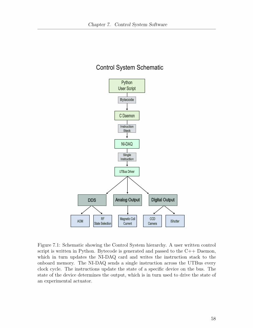
Chapter 7. Control System Software
Figure 7.1: Schematic showing the Control System hierarchy. A user written controlscript is written in Python. Bytecode is generated and passed to the C++ Daemon,which in turn updates the NI-DAQ card and writes the instruction stack to theonboard memory. The NI-DAQ sends a single instruction across the UTBus everyclock cycle. The instructions update the state of a specific device on the bus. Thestate of the device determines the output, which is in turn used to drive the state ofan experimental actuator.
58

Chapter 7. Control System Software
Figure 7.2: Module schematic showing the relation between the major componentsof the QDG Computer Control Program.
are named for storage and re-use, and can be arbitrarily nested to any depth. Thereare modules responsible for implementing commands to the DDS, the Analog Output,and the Digital Output, with a general UTBus module with functions common toall devices used across it. Further, there are modules with functions relating to thebytecode generation, and the managing of signals and events. The timing of eachmodule is self-enclosed in that it does not rely on any absolute external reference.Timing is relative to the beginning of the top level module; individual elements canbe moved in time either by altering the arrangement of the actions and directivesrelative to each other, by the inclusion of wait cycles, or by signifying a specific timeplacement relative to markers placed within the module. The state of each module issaved in a data file, this file is read during the recipe generation such that only thosesections of the module that alter the existing state are scheduled. This is beneficialin reducing the run time of individual experimental sequences.
The full extent of the system will not be presented here, this is done mainly forreasons of clarity; the subtleties inherent to much of the bytecode generation and tim-ing are inconsequential for writing and developing basic and high level experimentalscripts. What will be presented is the main hierarchy of modules, with the mostrelevant commands for each.
7.2.1 DDS module
This module contains functions relating to the DDS device. The DDS module is itselfa subclass of the UTBus Device module. A new DDS device is instantiated with thefollowing command
DDSName=DDS(address = DDSAddress,refclock = 15MHz,refclock multiplier = 20, internal FSK = False)
where DDSAddress corresponds to the 8-bit address of the unit. Once instantiated,the following commands can be used to change the state of the device.
59
Chapter 7. Control System Software
DDSName.reset()Resets the DDS device to the default values. There exists a reset functionality builtinto the AD9852 that this function uses. Often useful when initiating a DDS de-vice for the first time, or as a fall back option when the device does not seem to beworking properly. In the rare event that the device is not updating properly, andthe DDSName.reset() call has no effect, it might be necessary to manually delete thestate file for that device.
DDSName.set amplitude(Value)Sets the peak to peak amplitude of the cosine output. Requires a value between 0and 1 as the input. This function requires fewer instructions to be sent across the busthan many of the frequency functions. If it is desired that the output of a particularDDS be turned off, a call of DDSName.set amplitude(0.0) may be the simplest andquickest method.
DDSName.single tone(FrequencyValue)Programs the DDS to output a single frequency from the cosine output. Frequencyvalues from DC to 135MHz are valid, although it should be noted that the outputamplitude of frequencies above 110MHz decline rapidly with increasing frequency.
DDSName.unramped FSK(Frequency1,Frequency2)Requires two frequency values as input, where the first must be the lower of the two.Toggles between the two frequencies with a period equal to that of the TTL signalsent to the FSK input of the DDS unit. If this is used in conjunction with a MasterTable DDS, it is important that the DDSName.enable comp() call be used to ensurethat the onboard comparator is enabled. These particular DDS units require a sinewave signal to the FSK input.
DDSName.ramped FSK(Freq1,Freq2,FSK Period)Sets the DDS to run in a ramped frequency mode where the output varies in discretesteps from the initial frequency to secondary frequency and back in a continuousfashion. The period of the TTL signal used as the FSK reference is required in orderthat the step size be properly calculated. If this value is incorrect, it is possible thateither the full range of frequency values will not be reached, or that significant timeis spent at one of the boundary frequencies before the ramp is continued.
DDSName.enable comp()Enables the onboard comparator of the DDS unit. By default, the comparator isdisabled. Enabling the comparator is necessary for both the Master Table DDS unitsand the TTL DDS units.
DDSName.enable control DAC()Enables the output of the control DAQ. By default the control DAQ is disabled.Must be enabled for the TTL DDS units to function properly.
60
Chapter 7. Control System Software
7.2.2 Analog Output Module
This module contains functions relating to the Analog Output device. The moduleis itself a subclass of the UTBus Device module. A new AO device is instantiatedwith the following command
AOName=AnalogOutput(address= AOAddress)
where AOAddress corresponds to the 8-bit address of the unit. For simplicity, eachindividual output of a Analog Output board is treated as a unique device. Onceinstantiated, the following commands can be used to change the state of the device.
AOName.set scaled value(ScaledValue)The ScaledValue parameter represents the desired output voltage of the analog out-put channel between -10 and 10. This is a decimal number with 16-bit accuracy.
7.2.3 Digital Output Module
This module contains functions relating to the Digital Output device. The module isitself a subclass of the UTBus Device module. A new DO device is instantiated withthe following command
DOName=DigitalOutput(address = DOAddress)
where DOAddress corresponds to the 8-bit address of the unit.
DOName.set bit(Index, State)Sets the state of a single channel for a particular Digital Output device. Since theentire 16-bit register is rewritten during each update, the previous state of all 16channels are saved in a state file. When this function is called, the bit correspondingto the index of the output is changed with the saved states of the other bits heldunaltered. To set the 6th channel of a sample Digital Output device to a high statewould require SampleDO.set bit(5,1).
DOName.reset()Resets the state of all 16 channels to 0 (Low).As an aside, it is important to note that the DDS module has been programmedwith a hardware emulator that mimics the registers on the AD9852 DDS controller.The execution of a recipe results in a full update to the virtual registers, but onlythose instructions that alter the state of the physical DDS controller are includedin the bytecode sent across the UTBus. This is done as a means of optimizing theinstruction stack by reducing the number of instructions sent out across the UTBus.As an example, consider the case of a frequency update. A total of four registers areused to store the value of the frequency. If the difference between the new frequencyvalue and the old one is small, it may only be necessary to change the value storedin the least significant register. In this instance, only a single instruction, instead of
61

Chapter 7. Control System Software
four, would be sent across the UTBus. Although this method is useful in reducingbytecode chatter, it limits the ability to predict the exact time required for certainDDS instructions to be transferred via the UTBus. The only certainty is that thetime needed to update the DDS device will be less than or equal to the time neededto program the device from a reset state.
7.2.4 UTBus Device Module
A generic module composed of functions and characteristics common to all devicesacross the UTBus. The user does not use any of these functions directly when creatingan experimental control script.
7.2.5 Recipe Module
This module defines the recipe class, of which each user script is a subclass of. Arecipe is instantiated at the beginning of the script with the following command
R = Recipe(RecipeName, use internal clock=True,sampling frequency divider = 2000, use external trigger = False)
Further commands within the instantiation include the ability to set an externalclock set utbus external clock = Frequency. Once defined, R.start() marks the begin-ning of the control sequence, with R.end() marking the end. It is possible to includea delay within the instruction set through the use of the R.wait s(Time) command.Related to this call is also R.wait ms(Time) and R.wait us(Time).
7.2.6 User Defined Experimental Scripts
The user creates a ’Recipe’ script consisting of all the actions and scheduling directivesthat fully define a specific experimental control sequence. These scripts call functionsimported from the various modules that compose the QDG control software. Therequisite modules are loaded through the import command. For example, the DDSmodule is imported for use using
from UTBus1 import DDS (7.1)
where, in this case, ’UTBus1’ is the path where the modules are stored and representsthe first version of the UTBus.
The following is a sample script used for an experimental sequence in the MiniatureAtom Trap (MAT) experiment. It is a basic script, more complex scripts are possiblebut are beyond the scope of this thesis to discuss.
from math import sin,cos
import socket
import sys
62

Chapter 7. Control System Software
from UTBus1 import Recipe
from UTBus1 import AnalogOutput
from UTBus1 import DigitalOutput
from UTBus1 import DDS
KHz = 1000.
MHz = 1000000.
R = Recipe(r"D:\tmp\bcode.utb",
use_internal_clock=True,
sampling_frequency_divider=2000,
use_external_trigger=False)
R.start()
# ----------------- UT Bus Device instantiations ---------------
MATCoolingAOM = DDS(address=136,refclock=15*10**6,refclock_multiplier=20,
internal_FSK=False)
MATRepumpAOM = DDS(address=124,refclock=15*10**6,refclock_multiplier=20,
internal_FSK=False)
# ----------------- MAT DDS Setup for Synchronous detection ---------------
if 1:
fRepumpCenter = 80*MHz
fcenter = 80*MHz
df = 0*MHz
f2 = fcenter + df
f1 = fcenter - df
D = .00001
MATCoolingAOM.reset()
MATRepumpAOM.reset()
MATCoolingAOM.single_tone(f1)
MATRepumpAOM.single_tone(fRepumpCenter)
# This command produces a frequency ramp from f1 to f2 in D seconds
63

Chapter 7. Control System Software
MATCoolingAOM.ramped_FSK(f1,f2,D)
MATCoolingAOM.set_amplitude(0.7)
MATRepumpAOM.set_amplitude(0.7)
DO2 = DigitalOutput(address=255)
DO2.set_bit(7,1)
R.end()
64

Chapter 8
Measurements
8.1 MOT Optimization
Our experimental apparatus has been constructed to support the simultaneous trap-ping of Li and Rb atoms. Single species trapping of Rb atoms is a well establishedtechnique; as is shown by preliminary measurements of the steady state atom numberfor our system in a single species Rb MOT configuration [2].
The decision to trap Li atoms directly from an effusive source, without any in-termediary slowing mechanisms, requires a very careful determination of the steadystate atom number, the loading time, and the loading rate over the entire parameterspace of the experimental system. This is necessary not only to maximize the initialatom number, but also to determine if this method is viable as a means of eventuallygenerating ultracold molecules from a dual species MOT. The results, and discussion,that follow is specific to the performance of the Li MOT in absence of any Rb vapour.
8.1.1 Alignment
Originally, the cooling and trapping light in each axis was split by way of a polariza-tion beam splitter (PBS) to generate two beams propagating in opposite directions.This method allows for adjustments to be made to the intensity balance of each beampair, although this results in the total intensity of the incoming light being sharedacross the two beams.
Unfortunately, our Lithium slave lasers on the photoassociation table have outputpowers of only 28mW [60]. Methods of increasing the intensity are being discussed,but they could not be immediately implemented within the existing system. Insteadit was decided to resort to a retroreflection setup, where the cooling beams are sentdirectly through the trapping cell, then reflected back by way of retroreflecting mir-rors. This proved to be a simple way to essentially double the intensity of the coolinglight, giving atom numbers of approximately 2× 10⁷[2]. Due to the simplicity of theoptical components, this method makes it easier to spatially overlap the beams. Thereason this method was not used initially is that the intensity losses at each inter-face of the trapping cell result in an intensity imbalance between the beams. Thisimbalance pushes the center of the MOT away from the center of the magnetic field.
8.1.2 Atom Number Calibration
In general, the number of atoms in a MOT is related to the current signal from aphotodiode by
65

Chapter 8. Measurements
Natom =IPD
L · η ·R ·(hcλ· Γscatt
) (8.1)
where IPD is the current from the photodiode, L is the signal loss due to opticalcomponents, η is the collection efficiency of the detection system, R is the respon-sivity of the photodiode in millivolts. The signal loss due to optical components wascalculated to be L = 0.307. The light propagates through the trapping cell, twolenses, a dichroic mirror, and an interference filter before reaching the photodiode.The collection efficiency of the system is based on the solid angle of the imaging opticswith the MOT as the center. The lens is 75mm in diameter and is placed 11.8mmfrom the MOT, giving a value of η = 5.78 × 10⁻³. Finally, the responsivity of thephotodiode is R = 0.38A/W and is given as a manufacturer’s specification. For a2-level system, the scattering rate Γscatt is related to the frequency detuning (δ) ofthe cooling light by
0 1 2 3 4 5 6 7 8 9 1 0 1 1 1 2
2 . 0 x 1 0 5
4 . 0 x 1 0 5
6 . 0 x 1 0 5
8 . 0 x 1 0 5
Came
ra Sig
nal (C
ounts
)
P h o t o d i o d e S i g n a l ( m V )
C o r r e l a t e d D a t a L i n e a r F i t
Figure 8.1: The relationship between the fluorescence signal from the CCD cam-era and the photodiode. The photodiode signal has been calibrated with the atomnumber; a linear fit allows for the camera signal to be likewise converted.
Γscatt =Γ
2
s
1 + s+(
2δΓ
)2 (8.2)
where Γ is the natural linewidth of the atomic transition, and s = I/Isat. Table (8.1)gives the respective values for the atomic species used in our dual MOT experiment.Since the detection of a photon is predicate on an atom being trapped in the MOT,it is assumed that each signal event within a time period smaller than the scattering
66
Chapter 8. Measurements
rate corresponds to a single atom within the MOT. By factoring the total efficiencyof the detection system, we can determine a reasonable estimate of the atom numberfrom the signal from a photodiode.
Species Γ s
6Li (2π) · 5.87MHz 19.7
85,87Rb (2π) · 6.06MHz 14.8
Table 8.1: Natural linewidths and values of s = I/Isat for the atomic species used inour experiment.
This calibration calculation was worked through for a photodiode signal of IPD =VPD/1MΩ = 11nA, and detuning values of δ = δop = δor = (2π) × (−34MHz). Thenumber of atoms was found to be
Natom = 2.07× 10⁷ (8.3)
Using this value, it is possible to estimate the atom number of the MOT under otherconditions.
8.1.3 MOT Loading Model
The loading behaviour of a MOT determined by two parameters; the capture rate ofatoms into the trap, and the loss rate of atoms out of the trap. A simple differentialequation suffices in describing the time dependence of the trapped atom number
N = R− γN (8.4)
where N is the number of atoms, R is the loading rate, and γ is the loss rate due tocollisions with both background atoms such as Hydrogen, and hot, untrapped Li andRb atoms. Solving the differential equation for N gives
N =R
γ
(1− e−γt
)(8.5)
where we can define the value Nss = R/γ as the steady state atom number. Theloading time is defined as the inverse of the loss rate τ = 1/γ. This represents thetime required to fill the trap to the steady state atom number, as well as the averagetime an atom exists in the trap before being expelled through a collision event.
As shown in Fig. (8.2), the loading model fits the experimental data extremelywell.
8.1.4 Detuning
The frequencies of both the pump (cooling) and repump light greatly affects thenumber of atoms trapped in the MOT. The magnitude of the detuning from resonance
67

Chapter 8. Measurements
Figure 8.2: Fluorescence from a CCD camera was recorded every 500ms over theduration of the loading period of a Li MOT. The fluorescence was converted to atomnumber and fit using equation (8.5). The values of the parameters were found to beR = 1.1× 10⁶ and γ = 0.054. This corresponds to a loading time of τ = 18.2sec.
partially determines the maximum accessible velocity class of atoms. An empiricaldetermination of the optimum detunings δp and δr was performed by collecting dataon the fluorescence over the entire detuning space. A control script was writtento iteratively load a MOT and capture the fluorescence level using both a CCDcamera and a photodiode. The parameters δp, δr, and Icoil, where Icoil is the currentsupplied to the magnetic coils, were systematically varied during each iteration. Thefluorescence emitted by the trapped atoms in the MOT was recorded using both aphotodiode and a CCD camera. The photon count of the CCD camera is measuredby integrating over the pixel range of the image; because of this, the exposure timeof the camera must be taken into account when deriving quantities such as the atomnumber. Fig. (8.4) shows a sample comparison of the raw data at a magnetic coilcurrent of Icoil = 4A. Although the regions of maximum fluorescence do not coincideexactly, the spatial overlap suggests that a detuning of δp/(2π) = −34MHz andδr/(2π) = −25MHz should provide a maximized fluorescence signal.
In order to determine the atom number from the photon count of the camerasignal, it is necessary to first determine the relationship with respect to the photodiodevoltage signal. It was observed that the position of the MOT within the trapping cellchanged in relation to the frequencies of the light and the current to the magnetic coil.There was concern that this positional variation would cause the MOT image to straybeyond the capture range of the photodiode. Fortunately, the data suggests that thisconcern was unwarranted for this particular sequence. The best fit to the data isa linear equation that was then used to convert the camera signal to an equivalentvoltage.
The scattering rate, and hence the atom number, is dependent on the frequency
68

Chapter 8. Measurements
Figure 8.3: Atom number vs. laser detunings for increasing values of the magnetic coilcurrent (Icoil). The coil current is proportional to the magnetic field gradient. Notethe shift of the maximum atom number towards higher detuning values as the currentis increased. The peak atom number of 2.61× 10⁷ atoms is found at δp = −42MHz,δr = −44MHz, and Icoil = 7A. For our experiment a reference current of 2.84A wasmeasured to produce a magnetic field of 16.8G/cm.
detuning of the cooling light. Since both frequencies contribute to the cooling ofthe atoms, it was necessary to incorporate the changing values of δp and δr into thecalculation. It is clear that the actual value of Γscatt is bounded by those calculatedusing the minimum and the maximum of the detuning frequencies
Γscatt(Min[δp, δr]) ≤ Γscatt(δp, δr) ≤ Γscatt(Max[δp, δr]) (8.6)
In order to simplify the calculation, and to determine a lower bound on the atomnumber, the detuning that minimizes Γscatt was used. The atom number was thencalculated from
Natom =
[VCam
V refCam
]×[
ΓrefscattΓscatt(Min[δp, δr])
]× (2.07 · 107) (8.7)
69

Chapter 8. Measurements
Figure 8.4: Sample contour plots at Icoil = 4A showing the raw fluorescence data forboth the CCD camera signal and the photodiode signal.
where V refCam = 11mV and Γrefscatt = 2.45 · 106.
Fig.(8.3) shows the relationship between the atom number and the relative de-tunings of the pump and repump. It is clear that the values of the detunings thatmaximize the fluorescence signal are not necessarily those that maximize the atomnumber in the MOT. This means that there are two optimal detuning positions; thefirst where the atom number is largest, and the second where the fluorescence sig-nal is maximized. The former is used when loading a MOT, while the second canbe quickly shifted during a measurement in order to enhance the signal as much asneeded to make a measurement.
8.1.5 Intensity Dependence
The relative intensities of the pump and repump beams also are important in max-imizing the atom number of our Li MOT, as well as determining the need for anadditional amplification stage before the light is sent to the MOT. In this mea-surement, the frequency detunings were held fixed at δp = (2π) × (−34MHz) andδr = (2π)× (−25MHz), with a magnetic coil current of Icoil = 4A.
The intensities were adjusted through the use of an electro-optic modulator placedbetween the output port of the optical isolators of the Lithium slave lasers and a PBScube. In this way, both the pump and repump intensities could be independently con-trolled. Fig (8.5) shows the relationship to the atom number over the range of pumpand repump powers. The total atom numbers present at higher pump and repumppowers is promising, although the need for further amplification remains unresolved.The apparent plateau in the atom number as the pump power was changed may meanthat our existing system is adequate, but this is far from a definitive result. For the
70

Chapter 8. Measurements
Figure 8.5: Clockwise from top: (a) Contour plot showing the atom number presentin the MOT as a function of the light intensity of the pump and repump beams. (b)Increasing atom number for fixed pump power. (c) Increasing atom number for fixedrepump power
purposes of the first generation experiment, the output of the Lithium slave laserswill be left unmodified.
It is useful to determine the corresponding intensity values of the pump andrepump beams in each axis. In a retroreflection scheme, the reflected beam will incurgreater loss due to interactions with the trapping cell and mirror. Table (8.2) showsthe total intensities for the primary and reflected beams for the pump and repump inall three axes at maximum power values with corresponding transmission coefficients.The effect of the trapping cell on the intensity of the reflected beams, especially fors polarized light, is non-negligible. As stated earlier, this will reduce the efficiency ofthe cooling light, while also shifting the position of the atomic cloud relative to thezero field of the magnetic trap. Within the MOT, there exist fine structure changing
71

Chapter 8. Measurements
Beam Power Intensity Ts T 3s Tp T 3
p
(mW) (mW/cm2)
Pumpx 14.77 18.70 0.837 0.587 0.986 0.957Pumpy 5.83 7.38 0.837 0.587 0.986 0.957Pumpz 2.1 2.66 0.929 0.863 0.929 0.863
Repumpx 4.1 5.19 0.837 0.587 0.986 0.957Repumpy 4.3 5.44 0.837 0.587 0.986 0.957Repumpz 4.3 5.44 0.929 0.863 0.929 0.863
Table 8.2: Intensities of Pump and Repump Beams in each axis with primary andreflected beam transmission factors for both s and p polarizations. The transmissioncoefficient determines the intensity value of the light when it reaches the MOT.
collisions whereLi∗upper + Li→ Li∗lower + Li + Energy (8.8)
These collisions result in an increased velocity of the atom. According to [61], if theintensity of the cooling light is sufficiently high, it is possible to recapture the atomsfrom these fine-structure changing collisions. This recapture leads to heating in thetrap, but increases the equilibrium atom number. Currently, with the exception of theprimary pump beam in the x-axis, we are below the 15mW/cm2 intensity observedto produce a trap depth sufficient to contain the atoms from these collisions. Thismeans that we should continue to see gains from the recapture of these atoms as weincrease the intensity of beams in all three axes.
The total atom numbers present at higher pump and repump powers is promising,although the need for further amplification remains unresolved. The apparent plateauin the atom number as the pump power was changed may mean that our existingsystem is adequate, but this is far from a definitive result. For the purposes of the firstgeneration experiment, the output of the Lithium slave lasers will be left unmodified.
8.1.6 Oven Current
Finally, loading curves were taken for multiple oven currents and compensation z-coil current. This was done in order to determine the efficacy of our beam block inshielding the MOT from atoms escaping from the oven. The change in current changesthe vertical position of the atom cloud within the trapping region. If the beam blockis functioning as is expected, it is predicted that as the MOT is positioned beyondthe shielded trapping region, the loss rate due to collisions with hot Lithium atomsshould increase sharply. This would result in a sudden decrease in the loading timeof the MOT.
The oven temperature is controlled through a resistive heating element, and isdirectly related to the flux of atoms from the collimated beam source. Increasing theatom flux from the oven increases the number of atoms below the capture velocity ofthe MOT, but also increases the contribution from non-capturable atoms to collisional
72

Chapter 8. Measurements
losses. It is important to determine the oven current at which these various effectsare balanced.
8 . 0 8 . 5 9 . 0 9 . 5 1 0 . 0 1 0 . 5 1 1 . 00
1 02 03 04 05 06 0
8 . 0 8 . 5 9 . 0 9 . 5 1 0 . 0 1 0 . 5 1 1 . 001234567B
time c
onsta
nt Z _ - 2 Z _ 6 Z _ 0 Z _ 4 Z _ 2
AFlu
oresce
nce
(1E6 c
ounts
)
o v e n c u r r e n t ( A )
Figure 8.6: Fluorescence measurements and loading times determined as a functionof oven current for multiple compensation z-coil voltages. These voltages correspondto currents, which in turn correspond to magnetic fields. These magnetic fields de-termine the MOT position within the trapping cell. Higher oven currents result in alarger flux of atoms, but with an increased shift in the velocity profile. Altering thevoltage to the compensation z-coil shifts the MOT position relative to the center ofthe trapping field and was done to observe the effect of the beam block.
Fig.(8.6) demonstrates the effect of increasing oven temperature on both the load-ing time, and the fluorescence of the MOT. The fluorescence was measured on a Pix-elink CCD camera every 500ms, with an exposure time of 6ms, during the loadingstage of the MOT. When increasing the oven current, a time delay is required inorder allow the oven to reach temperature before taking further measurements. Eachdata point of the fluorescence corresponds to the value obtained after fully loadingthe MOT.
The expected decrease in the loading time as the MOT was positioned outside theshielded region of the trap was not observed. The loading times remained consistentacross all MOT positions at a given oven current. The fluorescence was maximized
73

Chapter 8. Measurements
at an oven current of 9.5A.
8.1.7 Conclusions
We have shown that loading from an effusive Lithium oven without the use of atraditional slowing mechanism is a viable method for producing atomic clouds inexcess of 107 atoms. Considering the size, cost, and experimental complexity ofincorporating a Zeeman slower into a vacuum system, this result is particularly usefulfor those situations where large atom numbers are not necessary within the contextof the experiment to be performed. It is possible that refinements in the secondgeneration experiment may lead to further gains.
Although this is a very promising result, the performance of the Li MOT withinthe context of a dual species system with Rb remains to be examined. It is expectedthat the added losses due to background collisions with the Rb atoms will decreasethe steady state atom number of the Li MOT, but the magnitude of this decline iscurrently unknown.
8.2 Ablation Loading
It has been demonstrated that intense UV or broad-band light can significantly in-crease the background vapour pressure of certain species of alkali atoms [62]. Thisprocess is due to light-induced atomic desorption (LIAD), and has been shown to pro-duce optically thick rubidium, potassium, and sodium atomic vapour. In a vapourcell, there exists a coating of alkali atoms on the inner surface. When light is incidenton the inner surface, the atoms present in this coating are quickly desorbed from thecell wall; resulting in an increased vapour pressure and a higher number of trappedatoms. Since the light can be shuttered quickly, this method can be used to buildlarge trap numbers while returning quickly to low background pressures.
Lithium atoms quickly adsorb to any available surface; the effusive atomic beamfrom our Li oven is blocked not only to create a sheltered region where the MOTresides, but also to limit the atoms from completely covering the optical access tothe trapping region. Although the block was designed to keep specific areas of thetrapping cell clean, there do exist regions of the cell where Li atoms from the ovenare deposited on the surface. Fig.(8.7) shows the accessible area of deposited Lithiumused in the desorption/ablation test.
Unlike Rubidium, the energy required to remove a Li atom from the adsorbedsurface layer is larger than that supplied by a diffuse UV source. Access to a pulsedYAG laser, frequency doubled to 532nm, led to an interest in determining the viabilityof loading the Lithium MOT from a desorption/ablation source instead of the effusiveoven.
8.2.1 Experimental Procedure
The frequency detunings were held fixed at δp = (2π)× (−34MHz) and δr = (2π)×(−25MHz), with the magnetic coil currents set to Icoil = 4A.
74

Chapter 8. Measurements
Figure 8.7: The adsorbed Lithium layer is present on all sides of the trapping cell,extending in a thin layer approximately 9mm past the position of the beam block.Ablation loading was tested first by directing the pulsed YAG light on the Lithium-Vacuum interface at the bottom of the cell (A), then by directing it on the Glass-Lithium interface at the top of the cell (B).
It is possible to trigger the pulsed YAG laser externally using a TTL signal. Thesignal was sent to the flashlamp input of the laser, with the Q-switch trigger setto trigger automatically from the flashlamp. Although this method introduces anincreased noise in the total pulse power and timing interval of the output, theseeffects were deemed inconsequential considering the nature of the test.
The magnetic coils were turned off, clearing the system of any residual trappedatoms. With the coils off, ten background images, one every 10ms with an exposuretime of 25ms, were taken as reference. The coils were then turned back on, with afurther 10 images taken at 500ms intervals. These images were taken to ensure thatthe Lithium oven had cooled sufficiently and was no longer contributing atoms to thesystem. At this point, a pulsed YAG laser (20mJ pulses at 10Hz) was triggered usinga Digital Output device. Images were collected from the Pixelink CCD camera every500ms for a 60s duration, at which point the laser was turned off. Images continuedto be taken every 500ms for a further 120s to measure the decay characteristics ofthe MOT.
A reference loading curve from the effusive Li oven was taken both as a comparisonof the efficiency of the ablation method, and as a calibration for converting the camerasignal to atom number, this is the data shown in Fig. (8.2).
Two positions were chosen for the ablation laser; the first on the lower surfaceof the trapping cell, so that the pulsed light was directed on the interface betweenthe vacuum and the deposited Lithium layer, and the second on the upper surface sothat the light was directed on the interface between the glass cell and the depositionlayer. Three separate trials were taken at each position; the beam alignment was leftunaltered to determine the effect of depletion on the loading rates.
75
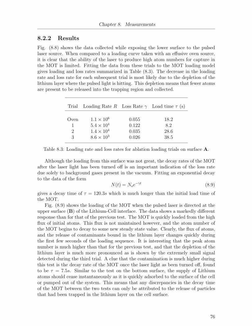
Chapter 8. Measurements
8.2.2 Results
Fig. (8.8) shows the data collected while exposing the lower surface to the pulsedlaser source. When compared to a loading curve taken with an effusive oven source,it is clear that the ability of the laser to produce high atom numbers for capture inthe MOT is limited. Fitting the data from these trials to the MOT loading modelgives loading and loss rates summarized in Table (8.3). The decrease in the loadingrate and loss rate for each subsequent trial is most likely due to the depletion of thelithium layer where the pulsed light is hitting. This depletion means that fewer atomsare present to be released into the trapping region and collected.
Trial Loading Rate R Loss Rate γ Load time τ (s)
Oven 1.1× 10⁶ 0.055 18.21 5.4× 10⁴ 0.122 8.22 1.4× 10⁴ 0.035 28.63 8.6× 10³ 0.026 38.5
Table 8.3: Loading rate and loss rates for ablation loading trials on surface A.
Although the loading from this surface was not great, the decay rates of the MOTafter the laser light has been turned off is an important indication of the loss ratedue solely to background gases present in the vacuum. Fitting an exponential decayto the data of the form
N(t) = Noe−γt (8.9)
gives a decay time of τ = 120.3s which is much longer than the initial load time ofthe MOT.
Fig. (8.9) shows the loading of the MOT when the pulsed laser is directed at theupper surface (B) of the Lithium-Cell interface. The data shows a markedly differentresponse than for that of the previous test. The MOT is quickly loaded from the highflux of initial atoms. This flux is not maintained however, and the atom number ofthe MOT begins to decay to some new steady state value. Clearly, the flux of atoms,and the release of contaminants bound in the lithium layer changes quickly duringthe first few seconds of the loading sequence. It is interesting that the peak atomnumber is much higher than that for the previous test, and that the depletion of thelithium layer is much more pronounced as is shown by the extremely small signaldetected during the third trial. A clue that the contamination is much higher duringthis test is the decay rate of the MOT once the laser light as been turned off, foundto be τ = 7.5s. Similar to the test on the bottom surface, the supply of Lithiumatoms should cease instantaneously as it is quickly adsorbed to the surface of the cellor pumped out of the system. This means that any discrepancies in the decay timeof the MOT between the two tests can only be attributed to the release of particlesthat had been trapped in the lithium layer on the cell surface.
76

Chapter 8. Measurements
8.2.3 Conclusions
The exact heating mechanisms and chemical composition of the deposition layers arenot well understood. As such, conjecture as to the processes by which the two verydifferent loading curves were created will be left for further review. The purpose of thetest was to determine the viability of laser ablation as a means of loading a LithiumMOT. To this end, laser ablation has been shown effective in quickly loading a smallatom number MOT while maintaining a very low residual gas vapour pressure. Unlikean oven source, this method allows for near instantaneous generation and cessationof background Lithium vapour.
Beyond the limited atom numbers, there are further concerns in regard to therandom direction of the Lithium atoms when vapourized in this manner. Great carehas been taken in the design of the effusive Lithium oven to ensure that contaminationof the optical access of the trapping cell is minimized.
77

Chapter 8. Measurements
0 20 40 60 80 100 120 140 160 180 200 220 240
0
1x10⁵
2x10⁵
3x10⁵
4x10⁵
5x10⁵
6x1050 10 20 30 40 50 60
0.0
3.0x10⁶
6.0x10⁶
9.0x10⁶
1.2x10⁷
1.5x10⁷
1.8x10⁷
YAG Light Off
YAG Ablation Tests: Bottom Surface (A)
YAG Light On
YAG Light On
Ato
m N
umbe
r
Oven Trial 1 Trial 2 Trial 3
Time (s)
Figure 8.8: Top: A Li MOT is loaded by means of laser ablation at the interfaceof the vacuum-Lithium layer, as well as from an effusive oven source. The laser istriggered at the 5 second mark. Bottom: Increased view of the loading and decaycurves of the laser ablation trials. The beam positon was held fixed throughout. Thelaser light is turned off 60 seconds after being triggered. The decay time for each ofthe three trial are calculated to be τ1 = 118.2s, τ2 = 120.3s, and τ3 = 119.2s.
78
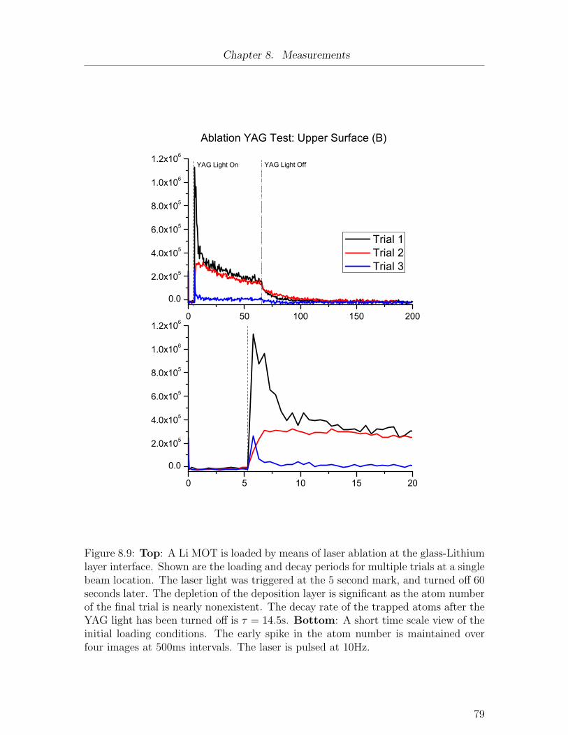
Chapter 8. Measurements
0 50 100 150 200
0.0
2.0x10⁵
4.0x10⁵
6.0x10⁵
8.0x10⁵
1.0x10⁶
1.2x10⁶
0 5 10 15 20
0.0
2.0x10⁵
4.0x10⁵
6.0x10⁵
8.0x10⁵
1.0x10⁶
1.2x10⁶
YAG Light Off
Trial 1 Trial 2 Trial 3
Ablation YAG Test: Upper Surface (B)
YAG Light On
Figure 8.9: Top: A Li MOT is loaded by means of laser ablation at the glass-Lithiumlayer interface. Shown are the loading and decay periods for multiple trials at a singlebeam location. The laser light was triggered at the 5 second mark, and turned off 60seconds later. The depletion of the deposition layer is significant as the atom numberof the final trial is nearly nonexistent. The decay rate of the trapped atoms after theYAG light has been turned off is τ = 14.5s. Bottom: A short time scale view of theinitial loading conditions. The early spike in the atom number is maintained overfour images at 500ms intervals. The laser is pulsed at 10Hz.
79
Bibliography
[1] Swati Singh. Progress towards ultra-cold ensembles of rubidium and lithium.Master’s thesis, University of British Columbia, 2007.
[2] Nina Rauhut. Towards ultracold LiRb molecules. Master’s thesis, Ludwig Max-imilians Universitat Munchen, 2007.
[3] Todd P. Meyrath and Florian Schreck. Digital RF synthesizer: DC to 135MHz.Technical report, Atom Optics Laboratory Center for Nonlinear Dynamics Uni-versity of Texas at Austin, 2005.
[4] Todd P. Meyrath and Florian Schreck. Octal 16-bit DAC. Technical report,Atom Optics Laboratory Center for Nonlinear Dynamics University of Texas atAustin, 2005.
[5] K.-A. Suominen. Theories for cold atomic collisions in light fields. Journal ofPhysics B Atomic Molecular Physics, 29:5981–6007, 1996.
[6] T.W. Hansch and A.L. Schawlow. Cooling of gases by laser radiation. OpticsCommunications, 13, January 1975.
[7] M. H. Anderson, J. R. Ensher, M. R. Matthews, C. E. Wieman, and E. A.Cornell. Observation of Bose-Einstein Condensation in a Dilute Atomic Vapor.Science, 269(5221):198–201, 1995.
[8] K. B. Davis, M. O. Mewes, M. R. Andrews, N. J. van Druten, D. S. Durfee,D. M. Kurn, and W. Ketterle. Bose-einstein condensation in a gas of sodiumatoms. Phys. Rev. Lett., 75(22):3969–3973, 1995.
[9] D. DeMille. Quantum computation with trapped polar molecules. Phys. Rev.Lett., 88(6), 2002.
[10] J.H. Eberly P.W. Milonni. Lasers. John Wiley and Sons, 1988.
[11] Y.B Ovchinnikov R. Grimm, M. Weidemller. Rev. Sci. Instrum., 42:95, 2000.
[12] C.J. Foot. Atomic Physics. Oxford University Press, 2005.
[13] P. D. Lett, W. D. Phillips, S. L. Rolston, C. E. Tanner, R. N. Watts, and C. I.Westbrook. Optical molasses. J. Opt. Soc. Am. B, 6(11):2084, 1989.
[14] E. L. Raab, M. Prentiss, Alex Cable, Steven Chu, and D. E. Pritchard. Trappingof neutral sodium atoms with radiation pressure. Phys. Rev. Lett., 59(23):2631–2634, 1987.
80

Bibliography
[15] Wolfgang Petrich, Michael H. Anderson, Jason R. Ensher, and Eric A. Cornell.Stable, tightly confining magnetic trap for evaporative cooling of neutral atoms.Phys. Rev. Lett., 74(17):3352–3355, 1995.
[16] H.J. Metcalf and P. van der Straten. Laser Cooling and Trapping. Springer,1999.
[17] Y. Castin, H. Wallis, and J. Dalibard. Limit of doppler cooling. J. Opt. Soc.Am. B, 6(11):2046, 1989.
[18] M. Weidemller and C. Zimmermann, editors. Interactions in Ultracold Gases.Wiley, 2003.
[19] Daniel A. Steck. Rubidium 87 d line data. Technical report, Los Alamos NationalLaboratory, 2001.
[20] P. D. Lett, R. N. Watts, C. I. Westbrook, W. D. Phillips, P. L. Gould, and H. J.Metcalf. Observation of atoms laser cooled below the doppler limit. Phys. Rev.Lett., 61(2):169–172, 1988.
[21] J. Dalibard and C. Cohen-Tannoudji. Laser cooling below the Doppler limit bypolarization gradients: Simple theoretical models. Journal of the Optical Societyof America B Optical Physics, 6:2023–2045, 1989.
[22] J. Lawall, F. Bardou, B. Saubamea, K. Shimizu, M. Leduc, A. Aspect, andC. Cohen-Tannoudji. Two-dimensional subrecoil laser cooling. Phys. Rev. Lett.,73(14):1915–1918, 1994.
[23] Mark Kasevich and Steven Chu. Laser cooling below a photon recoil with three-level atoms. Phys. Rev. Lett., 69(12):1741–1744, 1992.
[24] W. Ketterle and N.J. van Druten. Evaporative cooling of trapped atoms. Ad-vances in Atomic, Molecular, and Optical Physics, 37:181, 1996.
[25] Naoto Masuhara, John M. Doyle, Jon C. Sandberg, Daniel Kleppner, Thomas J.Greytak, Harald F. Hess, and Greg P. Kochanski. Evaporative cooling of spin-polarized atomic hydrogen. Phys. Rev. Lett., 61(8):935–938, 1988.
[26] A. G. Martin, K. Helmerson, V. S. Bagnato, G. P. Lafyatis, and D. E. Pritchard.rf spectroscopy of trapped neutral atoms. Phys. Rev. Lett., 61(21):2431–2434,1988.
[27] N. Balakrishnan and A. Dalgarno. Chemistry at ultracold temperatures. Chem.Phys. Lett., 341(5-6), 2001.
[28] J. J. Hudson, B. E. Sauer, M. R. Tarbutt, and E. A. Hinds. Measurementof the electron electric dipole moment using YbF molecules. Phys. Rev. Lett.,89(2):023003, 2002.
81

Bibliography
[29] D. Seidel and J.G. Muga. Ramsey interferometry with guided ultracold atoms.Eur. Phys. J. D, 41(1), 2007.
[30] R. deCarvalho, J.M. Doyle, B. Friedrich, T. Guillet, J. Kim, D. Patterson, andJ.D. Weinstein. Buffer-gas loaded magnetic traps for atoms and molecules: Aprimer. Eur. Phys. J. D, 7(3), 1999.
[31] Jinha Kim, Bretislav Friedrich, Daniel P. Katz, David Patterson, Jonathan D.Weinstein, Robert DeCarvalho, and John M. Doyle. Buffer-gas loading andmagnetic trapping of atomic europium. Phys. Rev. Lett., 78(19):3665–3668, 1997.
[32] Hendrick L. Bethlem, Giel Berden, and Gerard Meijer. Decelerating neutraldipolar molecules. Phys. Rev. Lett., 83(8):1558–1561, 1999.
[33] J. Doyle, B. Friedrich, R.V. Krems, and F. Masnou-Seeuws. Editorial: Quovadis, cold molecules? Eur. Phys. J. D, 31(2), 2004.
[34] H. R. Thorsheim, J. Weiner, and P. S. Julienne. Laser-induced photoassociationof ultracold sodium atoms. Phys. Rev. Lett., 58(23):2420–2423, 1987.
[35] John Weiner, Vanderlei S. Bagnato, Sergio Zilio, and Paul S. Julienne. Experi-ments and theory in cold and ultracold collisions. Rev. Mod. Phys., 71(1):1–85,1999.
[36] Y. B. Band and P. S. Julienne. Ultracold-molecule production by laser-cooledatom photoassociation. Phys. Rev. A, 51(6):R4317–R4320, 1995.
[37] Warren T. Zemke and William C. Stwalley. Long-range potential energy curvesfor the X1Σ+ and a3Σ+ states of NaRb. The Journal of Chemical Physics,114(24), 2001.
[38] H. Smith C.J. Pethick. BEC in dilute gases. Cambridge University Press, 2002.
[39] C. A. Stan, M. W. Zwierlein, C. H. Schunck, S. M. F. Raupach, and W. Ketterle.Observation of feshbach resonances between two different atomic species. Phys.Rev. Lett., 93(14):143001, 2004.
[40] S. Inouye, J. Goldwin, M. L. Olsen, C. Ticknor, J. L. Bohn, and D. S. Jin.Observation of heteronuclear feshbach resonances in a mixture of bosons andfermions. Phys. Rev. Lett., 93(18):183201, 2004.
[41] B. Deh, C. Marzok, C. Zimmermann, and P. W. Courteille. Feshbach resonancesin mixtures of ultracold 6Li and 87Rb gases. Phys. Rev. A, 77(1), January 2008.
[42] Thorsten Kohler, Krzysztof Goral, and Paul S. Julienne. Production of coldmolecules via magnetically tunable feshbach resonances. Reviews of ModernPhysics, 78(4):1311, 2006.
[43] S. J. J. M. F. Kokkelmans, H. M. J. Vissers, and B. J. Verhaar. Formation ofa bose condensate of stable molecules via a feshbach resonance. Phys. Rev. A,63(3):031601, 2001.
82

Bibliography
[44] R. V. Krems. Controlling collisions of ultracold atoms with dc electric fields.Physical Review Letters, 96(12), 2006.
[45] Michael E. Gehm. Properties of 6Li. Technical report, 2003.
[46] K. B. MacAdam, A. Steinbach, and C. Wieman. A narrow-band tunable diodelaser system with grating feedback, and a saturated absorption spectrometer forCs and Rb. American Journal of Physics, 60:1098–1111, December 1992.
[47] C. E. Wieman and L. Hollberg. Using diode lasers for atomic physics. Reviewof Scientific Instruments, 62:1–20, 1991.
[48] Cunyun Ye. Tunable External Cavity Diode Lasers. World Scientific, 2004.
[49] M. de Labachelerie and G. Passedat. Mode-hop suppression of littrow grating-tuned lasers. Appl. Opt., 32(3):269, 1993.
[50] A. S. Arnold, J. S. Wilson, and M. G. Boshier. A simple extended-cavity diodelaser. Review of Scientific Instruments, 69:1236–1239, March 1998.
[51] G.C. Bjorklund, M.D. Levenson, W. Lenth, and C. Ortiz. Frequency modu-lation (FM) spectroscopy. Applied Physics B: Lasers and Optics, 32:145–152,November 1983.
[52] G.L. Weissler and R.W. Carlson, editors. Methods of Experimental Physics:Vacuum Physics and Technology. Academic Press, 1979.
[53] G.F. Weston. Ultra-high Vacuum Practice. Butterworths, 1985.
[54] W. Becker. Vak. Tech., 7:149, 1958.
[55] Michael A. Joffe, Wolfgang Ketterle, Alex Martin, and David E. Pritchard.Transverse cooling and deflection of an atomic beam inside a zeeman slower.J. Opt. Soc. Am. B, 10(12):2257, 1993.
[56] Todd Meyrath. Electromagnetic design basics of cold atom experiments. Techni-cal report, Atom Optics Laboratory Center for Nonlinear Dynamics Universityof Texas at Austin, 2001.
[57] Paul Lebel. Contributions to the ubc quantum degenerate gas lab. Technicalreport, University of British Columbia, 2005.
[58] Todd P. Meyrath and Florian Schreck. A simple parallel bus computer controlsystem for atomic physics experiments. Technical report, Atom Optics Labora-tory Center for Nonlinear Dynamics University of Texas at Austin, 2004.
[59] Paul Lebel and Davy Mitchell. Ultrafast mechanical shutters for laser cooling ap-plication: the iShutter system. Technical report, University of British Columbia,2008.
83
Bibliography
[60] Janelle Van Dongen. Simultaneous cooling and trapping of 6Li and 85,87Rb.Master’s thesis, University of British Columbia, 2007.
[61] N. W. M. Ritchie, E. R. I. Abraham, Y. Y. Xiao, C. C. Bradley, R. G. Hulet,and P. S. Julienne. Trap-loss collisions of ultracold lithium atoms. Phys. Rev.A, 51(2):R890–R893, 1995.
[62] S. N. Atutov, R. Calabrese, V. Guidi, B. Mai, A. G. Rudavets, E. Scansani,L. Tomassetti, V. Biancalana, A. Burchianti, C. Marinelli, E. Mariotti, L. Moi,and S. Veronesi. Fast and efficient loading of a rb magneto-optical trap usinglight-induced atomic desorption. Phys. Rev. A, 67(5):053401, 2003.
84