Indigo

Blue

EXPERIMENT: VISIBLE LIGHT SPECTROSCOPY

In this experiment we will be investigating the color produced when light is absorbed by atransparent solution. The color a solution will appear to us can be predicted by using the colorwheel. If the chemicals in the solution absorb only red light, the solution will appear blue-green. Blue-green is the color directly opposite red on the color wheel. Colors opposite one another onthe color wheel are called complementary colors. Red and blue-green are complementary colors. If a solution appears blue then we would find that the chemicals are absorbing orange light sinceblue and orange are complementary. It should be noted that there is no such thing as purple light(purple is red + violet ) so if a solution is green it can’t absorb “purple” light. Instead it absorbsreds and violets.

We would also expect that as the concentration of the absorbing chemicals increase the amountof light absorbed would probably increase also. This relationship is called “Beer’s Law.” Theinstrument we will use to determine the type of light absorbed by the solution and the amount oflight absorbed is called a spectrometer.

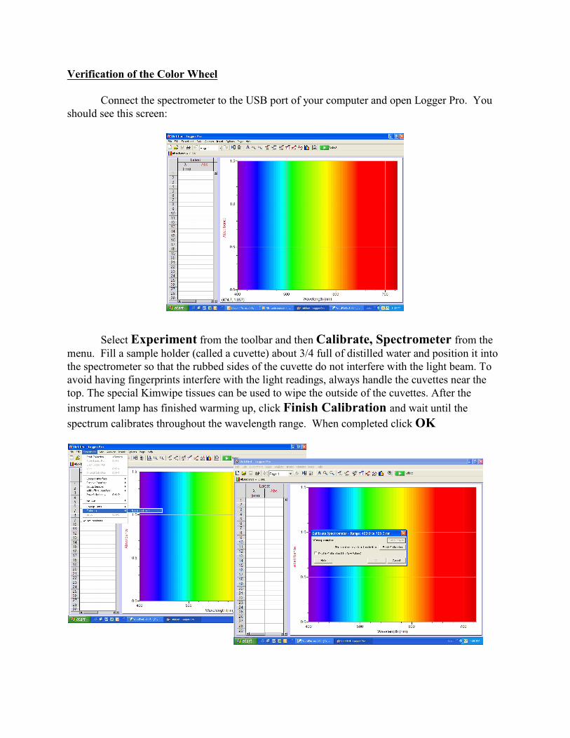
Verification of the Color Wheel

Connect the spectrometer to the USB port of your computer and open Logger Pro. Youshould see this screen:

Select Experiment from the toolbar and then Calibrate, Spectrometer from themenu. Fill a sample holder (called a cuvette) about 3/4 full of distilled water and position it intothe spectrometer so that the rubbed sides of the cuvette do not interfere with the light beam. Toavoid having fingerprints interfere with the light readings, always handle the cuvettes near thetop. The special Kimwipe tissues can be used to wipe the outside of the cuvettes. After the

instrument lamp has finished warming up, click Finish Calibration and wait until the

spectrum calibrates throughout the wavelength range. When completed click OK

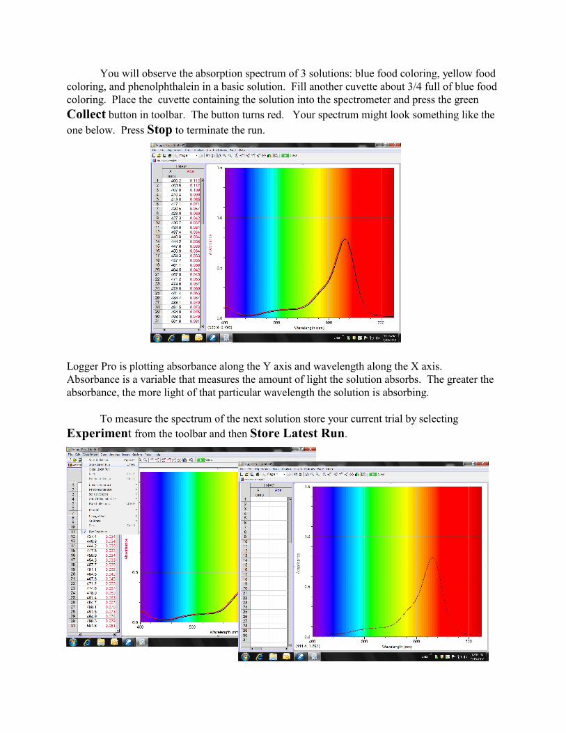
You will observe the absorption spectrum of 3 solutions: blue food coloring, yellow foodcoloring, and phenolphthalein in a basic solution. Fill another cuvette about 3/4 full of blue foodcoloring. Place the cuvette containing the solution into the spectrometer and press the green

Collect button in toolbar. The button turns red. Your spectrum might look something like the

one below. Press Stop to terminate the run.

Logger Pro is plotting absorbance along the Y axis and wavelength along the X axis. Absorbance is a variable that measures the amount of light the solution absorbs. The greater theabsorbance, the more light of that particular wavelength the solution is absorbing.

To measure the spectrum of the next solution store your current trial by selecting

Experiment from the toolbar and then Store Latest Run.

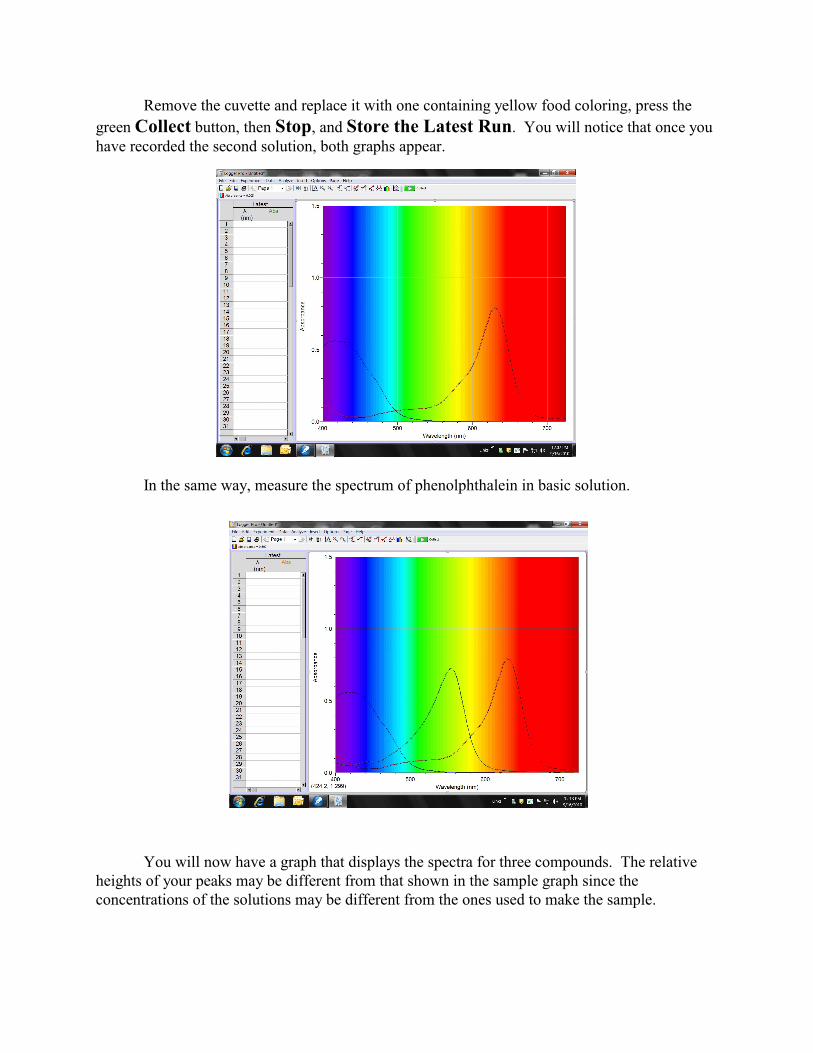
Remove the cuvette and replace it with one containing yellow food coloring, press the

green Collect button, then Stop, and Store the Latest Run. You will notice that once youhave recorded the second solution, both graphs appear.

In the same way, measure the spectrum of phenolphthalein in basic solution.

You will now have a graph that displays the spectra for three compounds. The relativeheights of your peaks may be different from that shown in the sample graph since theconcentrations of the solutions may be different from the ones used to make the sample.

Save your file to your computer and transfer the file to your lab

partner at this point. Each person needs to complete his/her own

graph modifications.

The Effect of Concentration on the Spectrum

You will measure the spectrum of distilled water and of four solutions of crystal violet. One solution will have been prepared for you and the concentration will be on the stock bottles. The three diluted solutions of crystal violet you will prepare. To prepare the diluted solutions,use pipets to add the quantities of solution shown in the table below to initially dry 50 mLbeakers. Stir the solutions thoroughly. Assume that the volumes are additive and in your Excelfile, calculate the molarity of crystal violet in each diluted solution. You now have 5 solutions:distilled water plus 4 solutions of crystal violet.

volume of crystal violet (mL) volume of water (mL)

10.00 5.00

10.00 10.00

5.00 10.00

Close your previous Logger Pro file and open a new one. Since this part of theexperiment is more quantitative than the first part of the experiment you want to be careful howthe cuvettes are placed into the spectrometer. The cuvette holder in the spectrometer is a littletoo large for the cuvettes (poor design) so that the cuvette can be rotated slightly in the holder. When you are positioning the cuvettes for this part of the experiment try to place them into theholder in as exactly the same position as you can. You will also see a small ink dot on the topedge of the cuvette. This is a reference mark that will allow to place the cuvette into the sampleholder so that the same side of the cuvette is facing the lamp for each trial.

Calibrate the spectrometer with distilled water as you did in the first part of theexperiment and record the spectrum of the distilled water. Pour out the distilled water and rinse

the cuvette with a few small portions of one of the crystal violet solutions. Be careful thatyou don’t use so much that you don’t have enough to fill the cuvette. Oncerinsed with solution, fill the cuvette with solution, wipe the cuvette with a tissue, place thecuvette into the sample holder with the same orientation of the reference mark, and record thespectrum. Pour out the crystal violet solution and rinse the cuvette with distilled water. Tomake sure all the crystal violet has been removed, rinse the cuvette with a small amount of 1 M

HCl. The acid will remove any crystal violet that has stained the cuvette. Thoroughly rinsethe cuvette with distilled water to remove all the acid. Then rinse and fill the cuvette with thenext crystal violet solution. Dry off the cuvette and record the spectrum. Repeat this process ofrinsing and filling until you have recorded the spectra for distilled water and the four crystalviolet solutions.

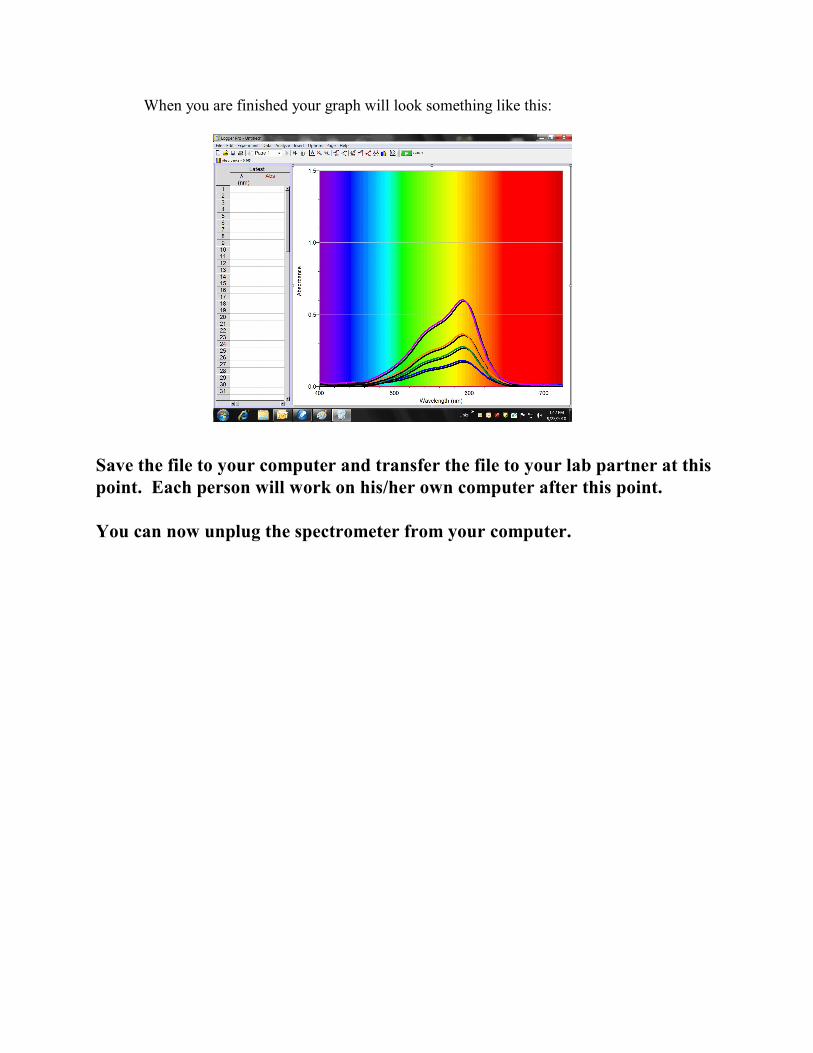
When you are finished your graph will look something like this:

Save the file to your computer and transfer the file to your lab partner at thispoint. Each person will work on his/her own computer after this point.

You can now unplug the spectrometer from your computer.

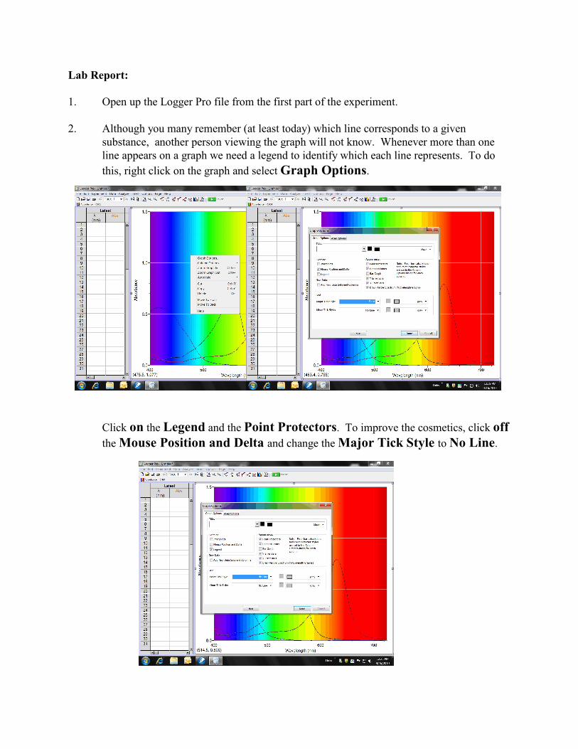
Lab Report:

1. Open up the Logger Pro file from the first part of the experiment.

2. Although you many remember (at least today) which line corresponds to a givensubstance, another person viewing the graph will not know. Whenever more than oneline appears on a graph we need a legend to identify which each line represents. To do

this, right click on the graph and select Graph Options.

Click on the Legend and the Point Protectors. To improve the cosmetics, click offthe Mouse Position and Delta and change the Major Tick Style to No Line.

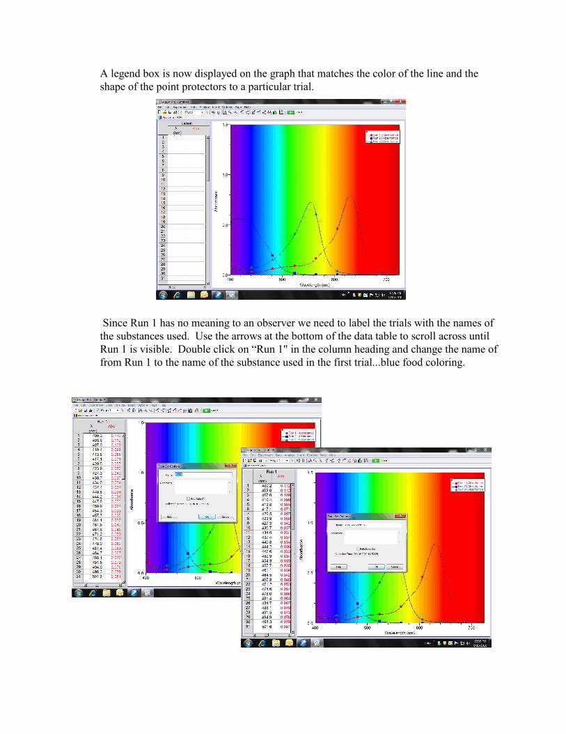
A legend box is now displayed on the graph that matches the color of the line and theshape of the point protectors to a particular trial.

Since Run 1 has no meaning to an observer we need to label the trials with the names ofthe substances used. Use the arrows at the bottom of the data table to scroll across untilRun 1 is visible. Double click on “Run 1" in the column heading and change the name offrom Run 1 to the name of the substance used in the first trial...blue food coloring.

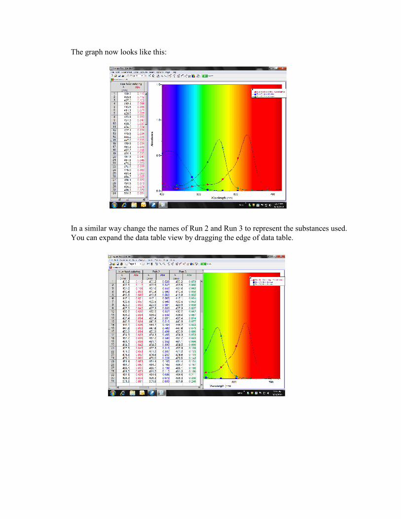
The graph now looks like this:

In a similar way change the names of Run 2 and Run 3 to represent the substances used. You can expand the data table view by dragging the edge of data table.

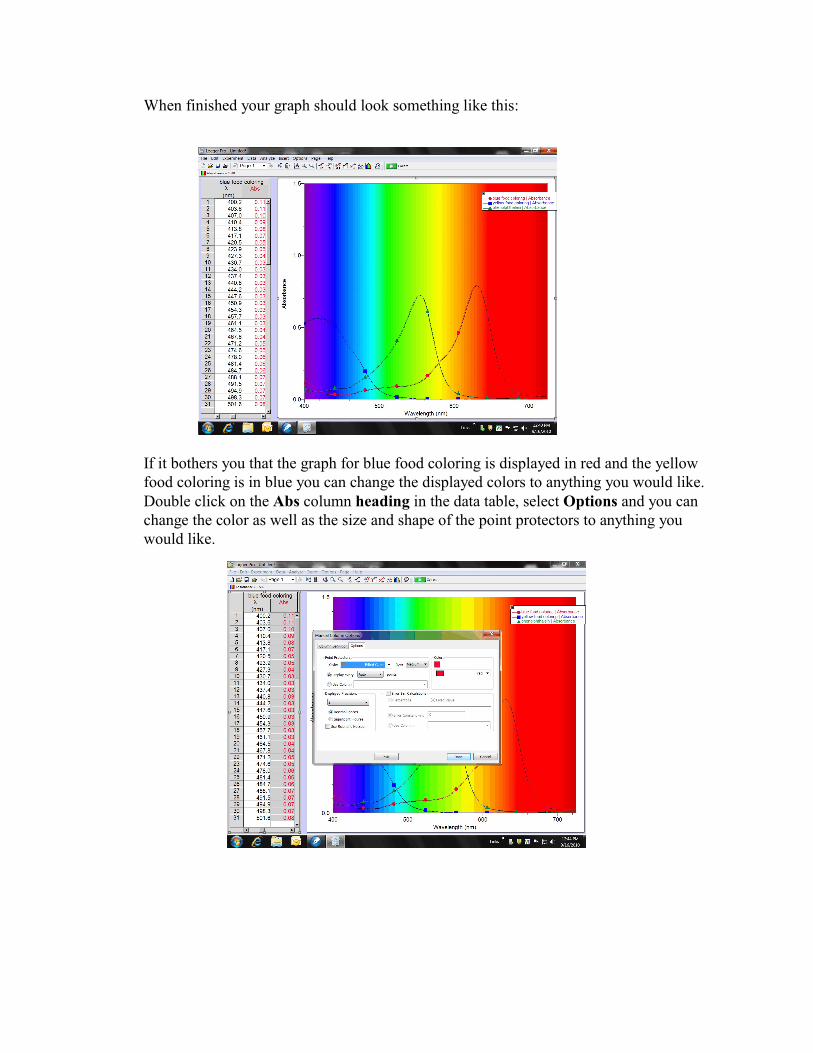
When finished your graph should look something like this:

If it bothers you that the graph for blue food coloring is displayed in red and the yellowfood coloring is in blue you can change the displayed colors to anything you would like. Double click on the Abs column heading in the data table, select Options and you canchange the color as well as the size and shape of the point protectors to anything youwould like.

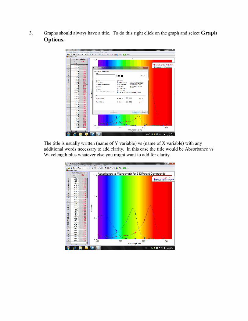
3. Graphs should always have a title. To do this right click on the graph and select GraphOptions.

The title is usually written (name of Y variable) vs (name of X variable) with anyadditional words necessary to add clarity. In this case the title would be Absorbance vsWavelength plus whatever else you might want to add for clarity.

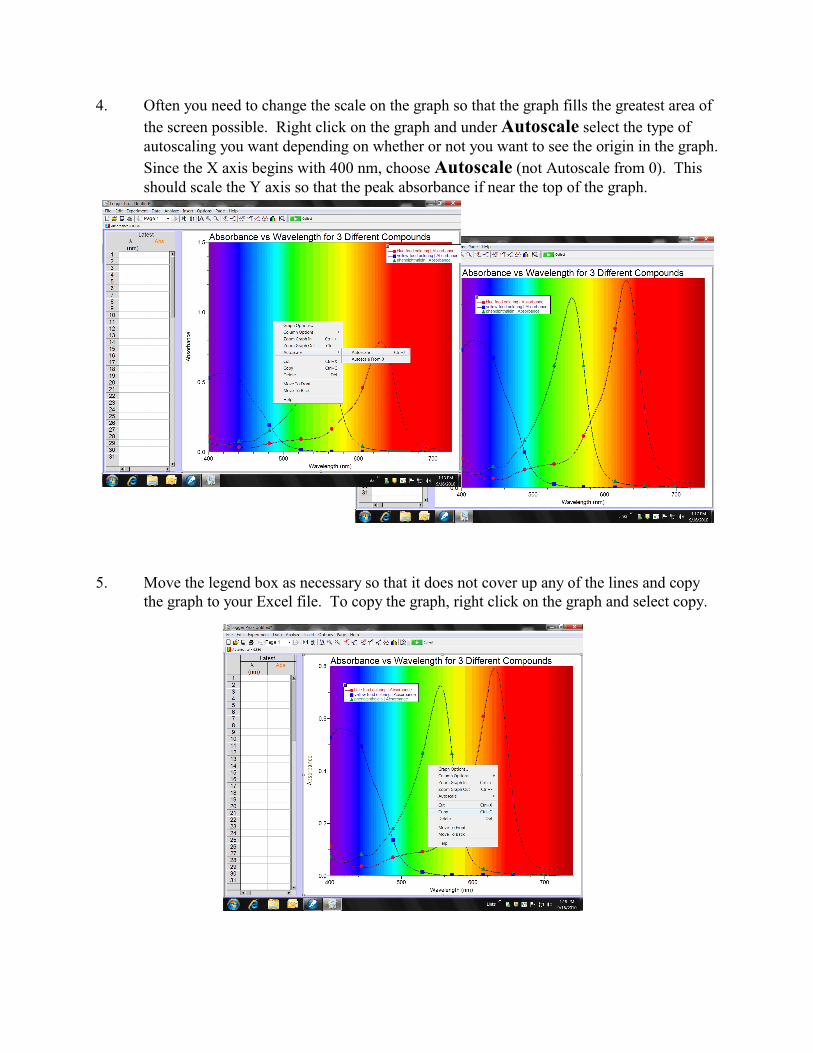
4. Often you need to change the scale on the graph so that the graph fills the greatest area of

the screen possible. Right click on the graph and under Autoscale select the type ofautoscaling you want depending on whether or not you want to see the origin in the graph.

Since the X axis begins with 400 nm, choose Autoscale (not Autoscale from 0). Thisshould scale the Y axis so that the peak absorbance if near the top of the graph.

5. Move the legend box as necessary so that it does not cover up any of the lines and copythe graph to your Excel file. To copy the graph, right click on the graph and select copy.

If your computer is a Mac, when the graph is copied, the colored background is retained. With PC computers the colored background is lost. Save your Logger Pro file to yourcomputer but do not send this modified file to your lab partner.

6. Record the observed colors of the three solutions in your Excel file.

7. Using the color wheel and the observed colors predict what colors you would expect thesolutions would absorb and enter those in the Excel file.

8. Use the background colors in your graph to determine the color each of the compoundsabsorbs most strongly (the peaks in the graph). Record these in your Excel file. Thesecolors should reasonably match those predicted from the color wheel.

9. Close your Logger Pro file and open the Logger Pro file from the second part of theexperiment.

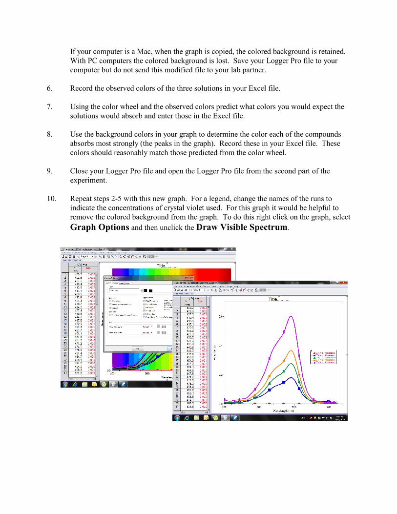
10. Repeat steps 2-5 with this new graph. For a legend, change the names of the runs toindicate the concentrations of crystal violet used. For this graph it would be helpful toremove the colored background from the graph. To do this right click on the graph, select

Graph Options and then unclick the Draw Visible Spectrum.

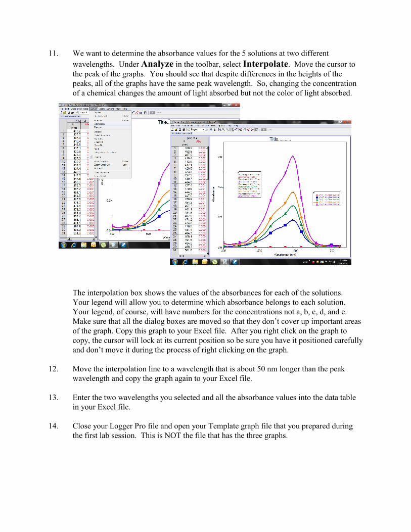
11. We want to determine the absorbance values for the 5 solutions at two different

wavelengths. Under Analyze in the toolbar, select Interpolate. Move the cursor tothe peak of the graphs. You should see that despite differences in the heights of thepeaks, all of the graphs have the same peak wavelength. So, changing the concentrationof a chemical changes the amount of light absorbed but not the color of light absorbed.

The interpolation box shows the values of the absorbances for each of the solutions. Your legend will allow you to determine which absorbance belongs to each solution. Your legend, of course, will have numbers for the concentrations not a, b, c, d, and e.Make sure that all the dialog boxes are moved so that they don’t cover up important areasof the graph. Copy this graph to your Excel file. After you right click on the graph tocopy, the cursor will lock at its current position so be sure you have it positioned carefullyand don’t move it during the process of right clicking on the graph.

12. Move the interpolation line to a wavelength that is about 50 nm longer than the peakwavelength and copy the graph again to your Excel file.

13. Enter the two wavelengths you selected and all the absorbance values into the data tablein your Excel file.

14. Close your Logger Pro file and open your Template graph file that you prepared duringthe first lab session. This is NOT the file that has the three graphs.

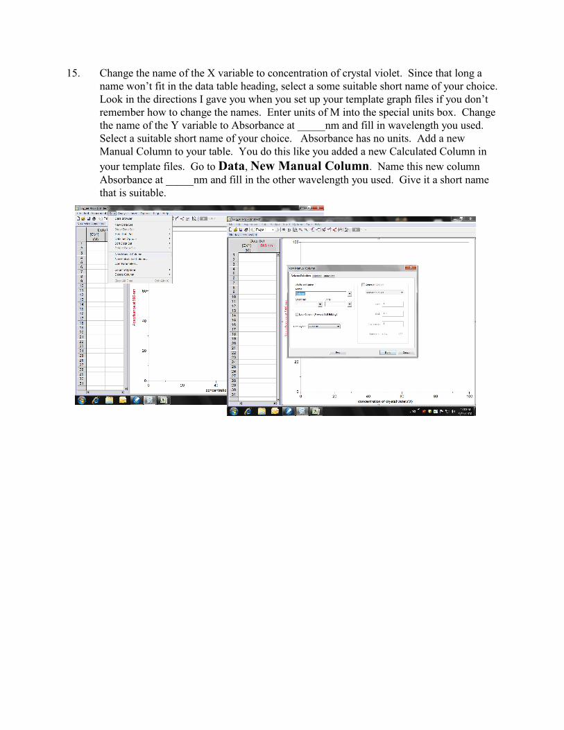
15. Change the name of the X variable to concentration of crystal violet. Since that long aname won’t fit in the data table heading, select a some suitable short name of your choice. Look in the directions I gave you when you set up your template graph files if you don’tremember how to change the names. Enter units of M into the special units box. Changethe name of the Y variable to Absorbance at _____nm and fill in wavelength you used. Select a suitable short name of your choice. Absorbance has no units. Add a new Manual Column to your table. You do this like you added a new Calculated Column in

your template files. Go to Data, New Manual Column. Name this new columnAbsorbance at _____nm and fill in the other wavelength you used. Give it a short namethat is suitable.

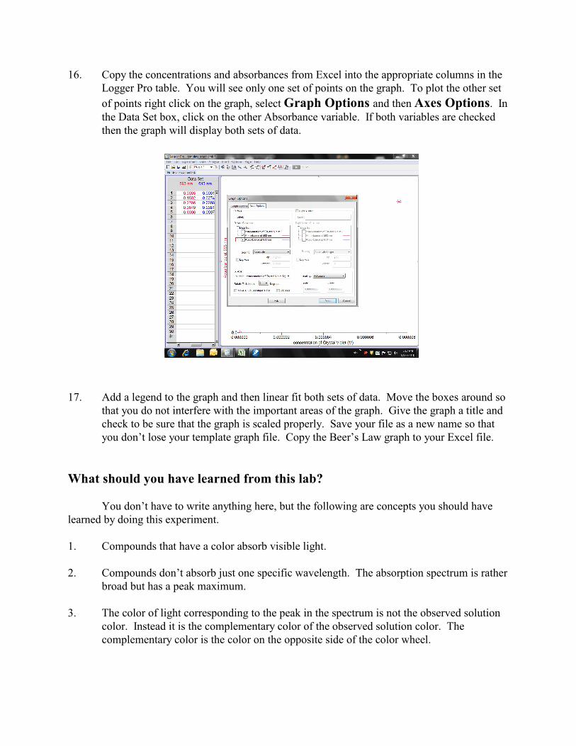
16. Copy the concentrations and absorbances from Excel into the appropriate columns in theLogger Pro table. You will see only one set of points on the graph. To plot the other set

of points right click on the graph, select Graph Options and then Axes Options. Inthe Data Set box, click on the other Absorbance variable. If both variables are checkedthen the graph will display both sets of data.

17. Add a legend to the graph and then linear fit both sets of data. Move the boxes around sothat you do not interfere with the important areas of the graph. Give the graph a title andcheck to be sure that the graph is scaled properly. Save your file as a new name so thatyou don’t lose your template graph file. Copy the Beer’s Law graph to your Excel file.

What should you have learned from this lab?

You don’t have to write anything here, but the following are concepts you should havelearned by doing this experiment.

1. Compounds that have a color absorb visible light.

2. Compounds don’t absorb just one specific wavelength. The absorption spectrum is ratherbroad but has a peak maximum.

3. The color of light corresponding to the peak in the spectrum is not the observed solutioncolor. Instead it is the complementary color of the observed solution color. Thecomplementary color is the color on the opposite side of the color wheel.

4. Absorbance is a variable that measures the amount of light absorbed. When theconcentration of the chemical is reduced the wavelength of the maximum absorptionremains the same but the absorbance decreases.

5. A graph of absorbance vs concentration is linear (Beer’s Law). The absorbance of asolution can be used to find the concentration of the chemical.

6. Beer’s Law graphs have different slopes depending on the wavelength used. The line willhave the greatest slope if the wavelength used is the one the compound absorbs moststrongly.