Experiment Manual - NetSimtetcos.com/downloads/VTU_Experiment_Manual_v8.3.pdf · Experiment Manual....
137
1 Experiment Manual
-
Upload
trinhduong -
Category
Documents
-
view
221 -
download
1
Transcript of Experiment Manual - NetSimtetcos.com/downloads/VTU_Experiment_Manual_v8.3.pdf · Experiment Manual....

1
Experiment Manual

2
The information contained in this document represents the current view of TETCOS on the
issues discussed as of the date of publication. Because TETCOS must respond to changing
market conditions, it should not be interpreted to be a commitment on the part of TETCOS,
and TETCOS cannot guarantee the accuracy of any information presented after the date of
publication.
This manual is for informational purposes only. TETCOS MAKES NO WARRANTIES,
EXPRESS, IMPLIED OR STATUTORY, AS TO THE INFORMATION IN THIS
DOCUMENT.
Warning! DO NOT COPY
Copyright in the whole and every part of this manual belongs to TETCOS and may not be
used, sold, transferred, copied or reproduced in whole or in part in any manner or in any
media to any person, without the prior written consent of TETCOS. If you use this manual
you do so at your own risk and on the understanding that TETCOS shall not be liable for any
loss or damage of any kind.
TETCOS may have patents, patent applications, trademarks, copyrights, or other intellectual
property rights covering subject matter in this document. Except as expressly provided in any
written license agreement from TETCOS, the furnishing of this document does not give you
any license to these patents, trademarks, copyrights, or other intellectual property. Unless
otherwise noted, the example companies, organizations, products, domain names, e-mail
addresses, logos, people, places, and events depicted herein are fictitious, and no association
with any real company, organization, product, domain name, email address, logo, person,
place, or event is intended or should be inferred.
Rev 8.3.10 (V), July 2015 (VTU_Karnataka), TETCOS. All rights reserved.
All trademarks are property of their respective owner.
Contact us at –
TETCOS
214, 39th A Cross, 7th Main, 5th Block Jayanagar,
Bangalore - 560 041, Karnataka, INDIA. Phone: +91 80 26630624
E-Mail: [email protected]
Visit: www.tetcos.com

3
Contents
Experiment 1: Introduction to NetSim network simulator & procedure of working in it. ................. 5
Experiment 2: Simulate a three nodes point – to – point network with duplex links
between them. Set the queue size and vary the bandwidth and find the number of packets
dropped ................................................................................................................................... 20
Experiment 3: Simulate a three node point-to-point network with the links connected
as follows: n0 n2, n1 n2 and n2 n3. Apply TCP agent between n0-n3 and UDP
between n1-n3. Apply relevant applications over TCP and UDP agents changing the
parameter and determine the number of packets sent by TCP / UDP. (n0, n1 and n3 are
nodes and n2 is router.). ....................................................................................................................... 28
Experiment 4: Simulate the different types of internet traffic such as FTP, TELNET over a
network and analyze the throughput. .................................................................................................. 36
Experiment 5: Simulate the transmission of ping messages over a network topology
consisting of 6 nodes and find the number of packets dropped due to congestion. ........................... 44
Experiment 6: Simulate an Ethernet LAN using n nodes (6-10), change error rate and
data rate and compare throughput. ..................................................................................................... 58
Experiment 7: To Simulate an Ethernet LAN using n nodes and set multiple traffic nodes
and determine collision across different nodes. .................................................................................. 71
Experiment 8: To Simulate an Ethernet LAN using n nodes and set multiple traffic nodes
and plot contention window for different source/destination. ........................................................... 75
Experiment 9: To simulate simple ESS and with transmitting nodes in wireless LAN by
simulation and determine the performance with respect to transmission of packets. ....................... 80
Experiment 10: Cyclic Redundancy Check -Write a program for error detecting code using
CRC-CCITT (16- bits). (Note: CRC 12, CRC 16 and CRC 32 are also available in NetSim) ....................... 88
Experiment 11: Sorting (Bubble Sort)- Write a program for frame sorting technique used
in buffers ................................................................................................................................... 97
Experiment 12: Distance Vector Routing - Implementation of distance vector routing
algorithm ................................................................................................................................. 102
Experiment 13: TCP/IP Sockets - Write Using TCP/IP sockets, write a client – server
program to make the client send the file name and to make the server send back the
contents of the requested file if present ............................................................................................ 108
Experiment 14: RSA - Write a program for simple RSA algorithm to encrypt and decrypt
the data ................................................................................................................................. 116

4
Experiment 15: Hamming Code - Write a program for Hamming code generation for
error detection and correction ........................................................................................................... 120
Experiment 16: Leaky Bucket Algorithm - Write a program for congestion control using
leaky bucket algorithm. ...................................................................................................................... 125
Appendix 1: Programming exercise -How to practice without NetSim............................................ 131
Appendix 2: Creating .exe file using Dev C++ .................................................................................... 135

5
Experiment 1:
Introduction to NetSim network simulator and
procedure of working in it.
Part A: Introduce students to network simulation through the
NetSim simulation package.
Theory:
What is NetSim?
NetSim is a network simulation tool that enables users to virtually create a network along
with its components such as devices, links, and applications etc. to study the behavior and
performance of the Network.
Some examples of its applications are
Protocol performance analysis
Application modelling and analysis
Network design and planning
Research and development of new networking technologies
Test and verification
What is simulation?
A simulation is the imitation of the operation of a real-world process or system over time.
Network simulation is a technique where a program models the behavior of a network either
by calculating the interaction between the different network entities (hosts/routers, data
links, packets, etc) using mathematical formulae, or actually capturing and playing back
observations from a production network.
The key features essential to any network simulation are -
Building the model – Create a network scenario with devices, links, applications etc

6
Running the simulation - Run the discrete event simulation (DES) and log different
performance metrics
Visualizing the simulation- Use a packet animator to view the flow of packets
Analyzing the results - Examine output performance metrics such as throughput,
delay, loss etc. at multiple levels - network, sub network, link, queue, application etc.
Developing your own protocol / algorithm - Extend existing algorithms by
modifying the simulators source C code
What does NetSim provide?
Simulation: NetSim provides simulation of various protocols working in various
networks as follows: Internetworks, Legacy Networks, BGP Networks, MPLS
Networks, Advanced Wireless Networks, Cellular Networks, Wireless Sensor
Networks, Personal Area Networks, LTE Networks and Cognitive Radio Networks.
Users can open, save, and delete experiments as desired. The different experiments can
also be analyzed using the analytics option in the simulation menu.
Programming: NetSim covers various programming exercises along with concepts,
algorithms, pseudo code and flowcharts. Users can also write their own source codes in
C/C++ and can link them to NetSim.
Some of the programming concepts are Address resolution protocol (ARP), Classless
inter domain routing (CIDR), Cryptography, Distance vector routing, shortest path,
Subnetting etc.
Utilities: This section handles the user management section used for adding/deleting
users, setting passwords etc.
Basics: Consists of Animated explanations of networking principles, protocol working
and packet formats.
Help: Consists of NetSim User Manual which displays all the Help related to NetSim.

7
Part B: Creating a Simple network, collecting and analyzing
statistics on network performance through the use of NetSim
This section will demonstrate how to create a basic network scenario and analyze in NetSim.
Analyzing a Network in NetSim mainly involves 5 steps
1. Create/Design the Network
2. Configure the Network
3. Model Traffic in the Network
4. Simulate
5. Analysis of Result
Opens the Simulation menu consisting of New, Open and Delete. User can simulate,
Internetworks, Legacy, Cellular, BGP, Advanced Wireless Networks, Wireless Sensor
Networks, Cognitive Radio Networks and LTE Networks
Opens the Programming menu where different
network programming lab exercises are available.
Menu to create users, set passwords, and
sample / exam mode. Switching of users can
be done through the login as option.
Displays all the Help related to
NetSim.
Consists of Animated explanations of
networking principles, protocol working
and packet formats.

8
Let us consider Internetworks. To create a new scenario, go to Simulation New
Internetworks
Perform the following steps to create a sample network scenario which looks like this:
9
1. Create/Design the Network
Step 1: Drop the devices
Click on Node icon and select Wired Node
Click on the environment (the grid in the center) where you want
the Wired Node to be placed. In this way, place two more wired
nodes.
Similarly to place a Switch and a Router, click on the respective device and click on the
environment at the desired location.

10
Step 2: Connecting devices on the environment
In order to connect devices present in the environment,
click on Link and select Wired Link.
Click and select the devices successively where link is
required. For example, select wired link and select Switch
and Router successively to connect them. In this manner,
continue to link all devices.
2. Configure the Network
Step 1: Configure Devices
Right click on the device and select properties

11
User can set values according to
requirement. Modify the properties of
any device and click on Accept.
In above scenario, default values
already present in the properties are
accepted.
Step 2: Configure Link
Right click on any Link and select
Properties.
User can set values
according to
requirement.
In above scenario,
default values
already present in
the properties are
accepted.
12
3. Model Traffic in the Network
After the network is configured, user needs to model traffic from Wired Node B to Wired
Node E.
Select the Application Button and click on the gap between the Grid Environment and the
ribbon. Now right click on Application and select Properties.
In above scenario, set Source_Id as 2(Wired Node B) and Destination_Id as 5(Wired Node
E). Click on Accept.

13
4. Simulate
For simulating the network scenario created, click on Run Simulation present in the Ribbon
Set the Simulation Time to 10 seconds. Select OK.

14
5. Analysis of Result
The different methods of performing analysis of Network performance in NetSim Academic
Version are
Performance Metrics
Packet Animation
Analytics (For multiple experiments)
5.1. Performance Metrics
NetSim provides distinct quantitative metrics at various abstraction levels such as Network
Metrics, Link Metrics, TCP Metrics, Application Metrics, etc at the end of simulation. With
the help of metrics, users can analyze the behavior of the modeled network and can compare
the impact of different algorithms on end-to-end behavior.
After simulation of a scenario is performed, the NetSim Performance Metrics are shown on
the screen as shown below
The Performance metrics can be further subdivided into sections
Network metrics: Here users can view the values of the metrics obtained based on
the overall network.
Link Metrics: Displays the values of the metrics pertaining to each link like Link_Id,
Packets_Transmitted, Error_Packets, Collided_Packets, Bytes_Transmitted,
Payload_Transmitted, Overhead_Transmitted.

15
Queue Metrics: Displays the values of the queue metrics for the devices containing
buffer queue like routers, access points etc.
Protocol metrics: Displays the protocol based metrics which are implemented in
Network scenario. Metrics will vary depending upon the type of network simulated.
Device metrics: Displays device related metrics like ARP table, IP forwarding tables.
This is also dependent upon the type of network
Application Metrics: Displays the various metrics based on the Application running
in the network scenario.
5.2 Packet Animation
NetSim provides the feature to play and record animations to the user. Packet animation
enables users to watch traffic flow through the network for in-depth visualization and
analysis.
User has the following options before running simulation:
Record the animation
Play and record animation while running simulation
No animation
The packet animation would then be recorded and the user can view the animation from the
metrics screen as shown below:
16
On clicking packet animation, a screen with the following toolbar appears:
While viewing packet animation, user can see the flow of packets as well as the type of
packet. Blue color packet denotes control packet, green color is used for data packet and red
color is error/collided packet.
Example showing packet animation: In first figure, Custom data packet is flowing from
Switch F to Node G (green color) and TCP_ACK is sent from Node G to Switch F in second
figure (blue color).
Click here to view packet animation
17
5.3 Analytics Menu (for multiple experiments)
Go to Simulation Analytics to view the Analytics screen. This module is designed to
enable comparison of performance metrics of multiple experiments. The metrics that can be
compared are Simulation Time, Packets Transmitted, Packets Errored, Packets Collided,
Bytes Transmitted, Payload Transmitted and Overhead Transmitted. Please note that other
metrics cannot be directly compared in the analytics menu, and an tool like Excel is
recommended.In Tool Bar, Click on the particular Network tab (Ex.- Internetworks, LTE
Networks etc) for comparing the performance of protocols under that Network.
For Internetworks, Advanced Wireless Networks – MANET, BGP Networks, Wireless
Sensor Networks, Personal Area Networks, LTE networks and Cognitive Radio
Networks,
1. Click Browse button select the Metrics.txt File inside the saved experiment folder
2. To add more experiments, repeat the above step for other experiments.
3. Select the Metrics - Select the coordinates for Y-axis by clicking on the dropdown
menu. User can select
4. Graph - Based on the X-axis (i.e. Metrics File/ Experiment selected) and Y-axis (i.e.
Metrics selected by using the dropdown menu above the graph), a Bar graph will be
plotted.
For Other Networks, select the Experiment based on the tab selected. When one of the
tabs is selected, all the experiments saved under the particular Network will be listed.
Click on the Experiment Name to add it onto the Metrics Table.

18
Saving an Experiment
For all Networks except Legacy Networks
Step 1: After simulation of the
network, on the top left corner
of Performance metrics screen,
click on the “Save Network and
Metric as” button
Step 2: Specify the Experiment Name and Save Path and click on OK
For Legacy Networks
Step 1: After simulation of the
network, on the top left corner
of Performance metrics screen,
click on the “Save Network and
Metric as” button
Step 2: Specify the Experiment Name and Comments and click on OK

19
Opening an Experiment
Open Network – All Networks except Legacy Networks
Go to Simulation Open Network menu
to open saved experiments. The following steps
need to be followed:
Click on Browse
Open the Saved experiment folder.
(NetSim creates a folder with the
experiment name during saving)
Select the configuration.xml file inside
the folder
Open Network – Legacy Networks
Go to Simulation Open Legacy Network
menu to open saved experiments. The following
steps need to be followed:
Select the User (Note: This option is
available in Admin login only)
Select the Network. Only Legacy Networks
option will be present.
Select the Protocol(Note: Protocols present
under Legacy Network will be displayed)
Select the Experiment
Click on Ok button to open the specified
Experiment.

20
Experiment 2:
Simulate a three nodes point – to – point network with
duplex links between them. Set the queue size and
vary the bandwidth and find the number of packets
dropped.
Theory:
Router forwards packets from one network to another network. When arrival rate of packets
is greater than the service (departure) rate, packets get buffered (queued). Once the buffer
(queue) is completely filled, all arriving packets will be dropped.
Procedure:
In NetSim, Select “Simulation New Internetworks”.
1. Create /Design the Network
Devices Required: 1 Router, 3 Wired Nodes
Network Diagram:
Note: While creating network, first
place the Router. Then place
Wired Node B, C and D as shown
here.
Connect Wired Node B
with Router first. Then connect
Wired Node C and Wired Node D
with Router

21
2. Configure the Network (Sample 1)
Wired Node Properties:
Disable TCP in Wired Node B.
Right Click Wired Node B Properties
Router Properties: Right click on Router Properties. Set buffer size to 8 MB. Accept
default values for remaining parameters.
Wired Link Properties: Right click on Wired Link Properties and set the values.
Link Properties Wired Link 1 Wired Link 2
Uplink Speed (Mbps) 10 10
Downlink Speed (Mbps) 10 10
Uplink BER No Error No Error
Downlink BER No Error No Error

22
3. Model Traffic in the Network (Sample 1)
Select the Application Button and click on the gap between the Grid Environment and the
ribbon. Now right click on Application and select Properties.
Application Properties: Modify the Application properties as specified in the left table.
4. Simulate
Simulation Time - 100 Sec
After completion of the experiment, “Save” the experiment for future analysis of results.
Application Type Custom
Source ID 2 (Wired Node B)
Destination ID 3 (Wired Node C)
Packet Size
Distribution Constant
Value(Bytes) 1460
Inter Arrival Time
Distribution Constant
Value(µs) 1200

23
Steps to save an experiment:
Step 1: After simulation of the
network, on the top left corner
of Performance metrics screen,
click on the “Save Network and
Metric as” button
Step 2: Specify the Experiment Name and Save Path and click on OK
5. Configure the Network (Sample 2)
Follow all the steps as shown in Sample 1 and modify only the wired link properties as
shown below.
OR
User can also select the “Go back to Network” option, select the Edit button and modify
only the wired link properties as shown below.
Wired Link Properties: Right click on Wired Link Properties and set the values.
Link Properties Wired Link 1 Wired Link 2
Uplink Speed (Mbps) 10 8.448
Downlink Speed (Mbps) 10 8.448
Uplink BER No Error No Error
Downlink BER No Error No Error
6. Simulate
Simulation Time - 100 Sec
After completion of the simulation, “Save” the experiment for future analysis of results.
24
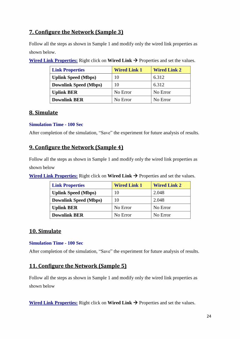
7. Configure the Network (Sample 3)
Follow all the steps as shown in Sample 1 and modify only the wired link properties as
shown below.
Wired Link Properties: Right click on Wired Link Properties and set the values.
Link Properties Wired Link 1 Wired Link 2
Uplink Speed (Mbps) 10 6.312
Downlink Speed (Mbps) 10 6.312
Uplink BER No Error No Error
Downlink BER No Error No Error
8. Simulate
Simulation Time - 100 Sec
After completion of the simulation, “Save” the experiment for future analysis of results.
9. Configure the Network (Sample 4)
Follow all the steps as shown in Sample 1 and modify only the wired link properties as
shown below
Wired Link Properties: Right click on Wired Link Properties and set the values.
Link Properties Wired Link 1 Wired Link 2
Uplink Speed (Mbps) 10 2.048
Downlink Speed (Mbps) 10 2.048
Uplink BER No Error No Error
Downlink BER No Error No Error
10. Simulate
Simulation Time - 100 Sec
After completion of the simulation, “Save” the experiment for future analysis of results.
11. Configure the Network (Sample 5)
Follow all the steps as shown in Sample 1 and modify only the wired link properties as
shown below
Wired Link Properties: Right click on Wired Link Properties and set the values.

25
Link Properties Wired Link 1 Wired Link 2
Uplink Speed (Mbps) 10 1.54
Downlink Speed (Mbps) 10 1.54
Uplink BER No Error No Error
Downlink BER No Error No Error
12. Simulate
Simulation Time - 100 Sec
After completion of the simulation, “Save” the experiment for future analysis of results.
13. Configure the Network (Sample 6)
Follow all the steps as shown in Sample 1 and modify only the wired link properties as
shown below
Wired Link Properties: Right click on Wired Link Properties and set the values.
Link Properties Wired Link 1 Wired Link 2
Uplink Speed (Mbps) 10 0.064
Downlink Speed (Mbps) 10 0.064
Uplink BER No Error No Error
Downlink BER No Error No Error
14. Simulate
Simulation Time - 100 Sec
After completion of the simulation, “Save” the experiment for future analysis of results.
15. Analysis of Result
Go to Simulation Open Metrics menu to open the results of saved experiments.

26
Click on Browse and select the Metrics.txt file (present with the saved experiment) you want
to open
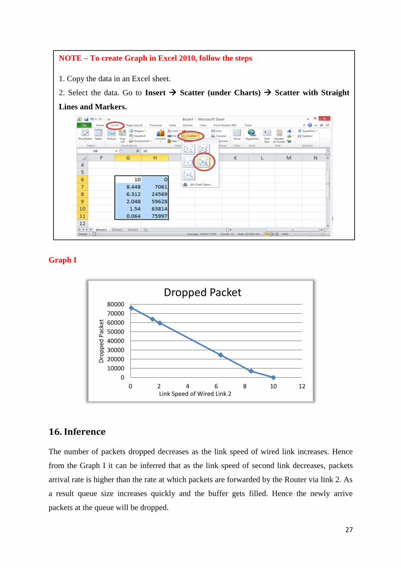
Open the Metrics.txt file of the first saved sample and note down the “Dropped Packet”
values of Port Id=2 available under “Queue Metrics” in an Excel file.
Similarly please follow the same steps for all the saved experiments and note down the
Dropped Packets values and Wired Link 2 speed of that sample. It will be as shown below.
Sample
Number
Link Speed of Wired
Link2 (Mbps)
Number of packets
dropped
1 10 0
2 8.448 7061
3 6.312 24569
4 2.048 59628
5 1.54 63814
6 0.064 75997
27
Graph I
16. Inference
The number of packets dropped decreases as the link speed of wired link increases. Hence
from the Graph I it can be inferred that as the link speed of second link decreases, packets
arrival rate is higher than the rate at which packets are forwarded by the Router via link 2. As
a result queue size increases quickly and the buffer gets filled. Hence the newly arrive
packets at the queue will be dropped.
0
10000
20000
30000
40000
50000
60000
70000
80000
0 2 4 6 8 10 12
Dro
pp
ed P
acke
t
Link Speed of Wired Link 2
Dropped Packet
NOTE – To create Graph in Excel 2010, follow the steps
1. Copy the data in an Excel sheet.
2. Select the data. Go to Insert Scatter (under Charts) Scatter with Straight
Lines and Markers.

28
Experiment 3:
Simulate a three node point-to-point network with the
links connected as follows: n0 n2, n1 n2 and n2
n3. Apply TCP agent between n0-n3 and UDP
between n1-n3. Apply relevant applications over TCP
and UDP agents changing the parameter and
determine the number of packets sent by TCP / UDP.
(n0, n1 and n3 are nodes and n2 is router.).
Theory:
TCP:
TCP recovers data that is damaged, lost, duplicated, or delivered out of order by the internet
communication system. This is achieved by assigning a sequence number to each octet
transmitted, and requiring a positive acknowledgment (ACK) from the receiving TCP. If the
ACK is not received within a timeout interval, the data is retransmitted. At the receiver side
sequence number is used to eliminate the duplicates as well as to order the segments in
correct order since there is a chance of “out of order” reception. Therefore, in TCP no
transmission errors will affect the correct delivery of data.
UDP:
UDP uses a simple transmission model with a minimum of protocol mechanism. It has no
handshaking dialogues, and thus exposes any unreliability of the underlying network protocol
to the user's program. As this is normally IP over unreliable media, there is no guarantee of
delivery, ordering or duplicate protection.
Procedure: In NetSim, Select “Simulation New Internetworks”.

29
1. Create /Design the Network
Devices Required: 1 Router, 3 Wired Nodes
Network Diagram:
2. Configure the Network (Sample 1)
Wired Node Properties:
Disable TCP in Wired Node B.
Right Click Wired Node B Properties
Disable UDP in Wired Node C.
Right Click Wired Node C Properties
Note: While creating network, first
place the Router. Then place
Wired Node B, C and D as shown
here.
Connect Wired Node B
with Router first. Then connect
Wired Node C and Wired Node D
with Router

30
3. Model Traffic in the Network (Sample 1)
Select the Application Button and click on the gap between the Grid Environment and the
ribbon. Now right click on Application and select Properties.
NOTE: The procedure to create multiple applications are as follows:
Step 1: Click on the ADD button present in the bottom left corner to add a new application.

31
Application Properties:
Create two (2) Application and set the values as shown below.
Application Type Custom Custom
Source ID 2(Wired Node B) 3(Wired Node C)
Destination ID 4(Wired Node D) 4(Wired Node D)
Packet Size
Distribution Constant Constant
Value(Bytes) 1460 1460
Inter Arrival Time
Distribution Constant Constant
Value(µs) 10000 10000
4. Simulate
Simulation Time - 100 Sec
After completion of the experiment, “Save” the experiment for future analysis of results.
Steps to save an experiment:
Step 1: After simulation of the
network, on the top left corner
of Performance metrics screen,
click on the “Save Network and
Metric as” button
Step 2: Specify the Experiment Name and Save Path and click on OK

32
5. Model Traffic in the Network (Sample 2)
Follow all the steps as shown in Sample 1 and modify only the Application properties as
shown below .
OR
User can also select the “Go back to Network” option, select the Edit button and modify
only the Application properties as shown below.
Application Properties:
Create 2 Application and set the values as shown below
Application Type Custom Custom
Source ID 2(Wired Node B) 3(Wired Node C)
Destination ID 4(Wired Node D) 4(Wired Node D)
Packet Size
Distribution Constant Constant
Value(Bytes) 1460 1460
Inter Arrival Time
Distribution Constant Constant
Value(µs) 5000 5000
6. Simulate
Simulation Time - 100 Sec
After completion of the simulation, “Save” the experiment for future analysis of results.
7. Model Traffic in the Network (Sample 3)
Follow all the steps as shown in Sample 1 and modify only the Application properties as
shown below

33
Application Properties:
Create 2 Application and set the values as shown below
Application Type Custom Custom
Source ID 2(Wired Node B) 3(Wired Node C)
Destination ID 4(Wired Node D) 4(Wired Node D)
Packet Size
Distribution Constant Constant
Value(Bytes) 1460 1460
Inter Arrival Time
Distribution Constant Constant
Value(µs) 2500 2500
8. Simulate
Simulation Time - 100 Sec
After completion of the simulation, “Save” the experiment for future analysis of results.
9. Analysis of Result
Go to Simulation Open Metrics menu to open the results of saved experiments.
Click on Browse and select the Metrics.txt file (present with the saved experiment) you want
to open

34
Open the Metrics.txt file and note the Number of
Segments Sent, Segments Received available in the
Connection Metrics under TCP Metrics and
Datagram Sent, Datagram Received available in the
UDP Metrics of “Performance Metrics” screen of
NetSim in an Excel file. Do the same procedure for
the rest 5 samples.
Graph I
(Note: The “Packets transmitted successfully” for TCP is Segments Received and for UDP
is Datagram Received of the destination node i.e., Wired Node 3)
Number of packets transmitted successfully in TCP and UDP
0
5000
10000
15000
20000
25000
30000
35000
40000
45000
10000 5000 2500
Pac
kets
tra
nsm
itte
d s
ucc
ess
fully
Inter arrival time (Micro Sec)
TCP vs UDP
TCP
UDP
NOTE – To create Graph in Excel 2010, follow the steps
1. Copy the data in an Excel sheet.
2. Select the data. Go to Insert Column (under Charts) Clustered Column.

35
Graph II
Number of lost packets in TCP and UDP
(Note: To get the “No. of packet lost”, For TCP, get the difference between Segments Sent
and Segments Received and for UDP, get the difference between Datagram Sent and
Datagram Received)
10. Inference
Graph I, shows that the number of successful packets transmitted in TCP is greater than (or
equal to) UDP. Because, when TCP transmits a packet containing data, it puts a copy on a
retransmission queue and starts a timer; when the acknowledgment for that data is received,
the segment is deleted from the queue. If the acknowledgment is not received before the
timer runs out, the segment is retransmitted. So even though a packet gets errored or dropped
that packet will be retransmitted in TCP, but UDP will not retransmit such packets.
As per the theory given and the explanation provided in the above paragraph, we see in
Graph 2, that there is no packet loss in TCP but UDP has packet loss.
0
100
200
300
400
500
600
700
800
900
1000
Exp1 Exp2 Exp3
No.o
f pac
ket
lost
Experiment list
TCP vs UDP
TCP
UDP

36
Experiment 4:
Simulate the different types of internet traffic such as
FTP, TELNET over a network and analyze the
throughput.
Theory:
FTP is File Transfer Protocol that transfers the files from source to destination. It is an
application layer protocol. The file transfer takes place over TCP.
TELNET is Terminal Network Protocol that is used to access the data in the remote machine.
It is also an Application layer protocol. It establishes connection to the remote machine over
TCP.
FTP, Database, Voice, HTTP, Email, Peer to Peer and Video are the traffic types available as
options in NetSim. To model other applications the “Custom” option is available. TELNET
application has been modeled in NetSim by using custom traffic type. Packet Size and Packet
Inter Arrival Time for TELNET application is shown below:
Packet Size
Distribution Constant
Packet Size (Bytes) 1460
Packet Inter Arrival Time
Distribution Constant
Packet Inter Arrival Time (µs) 15000
Procedure:
In NetSim, Select “Simulation New Internetworks”.
1. Create /Design the Network
Devices Required: 3 Routers, 8 Wired Nodes

37
Network Diagram:
2. Configure the Network (Sample 1)
Wired Node Properties:
TCP should be enabled in all Wired Nodes.
Wired Link Properties: Right click on Wired Link Properties and set the values.
Link Properties All Wired Link
Uplink Speed (Mbps) 1
Downlink Speed (Mbps) 1
Uplink BER No Error
Downlink BER No Error
Note: While creating network, place the devices according to the Node ID given in
diagram above in order to easily understand the settings to be configured as provided in
this manual.
For example: Figure shows Wired Node A has Node ID 1 and Wired Node B has Node
ID 2.So first place a Wired Node at the location of Wired Node A and then at Wired
Node B and so on.

38
3. Model Traffic in the Network (Sample 1)
Select the Application Button and click on the gap between the Grid Environment and the
ribbon. Now right click on Application and select Properties.
Application Properties:
Application Type FTP
Source ID 4(Wired Node D)
Destination ID 5(Wired Node E)
File Size
Distribution Constant
Size (Bytes) 10000000
File Inter Arrival Time
Distribution Constant
Inter Arrival Time 10 sec
4. Simulate
Simulation Time - 100 Sec
After completion of the experiment, “Save” the
experiment for future analysis of results.
Steps to save an experiment:
Step 1: After simulation of the network, on the
top left corner of Performance metrics screen,
click on the “Save Network and Metric as” button.
Step 2: Specify the Experiment Name and
Save Path and click on OK

39
5. Model Traffic in the Network (Sample 2)
Follow all the steps as shown in Sample 1 and modify only the Application properties as
shown below
OR
User can also select the “Go back to Network” option, select the Edit button and modify
only the Application properties as shown below.
Application Properties:
Application Type FTP Custom(for TELNET)
Source ID 4(Wired Node D) 1(Wired Node A)
Destination ID 5(Wired Node E) 6(Wired Node F)
File Size Packet Size
Distribution Constant Constant
Size (Bytes) 10000000 1460
File Inter Arrival Time Packet Inter Arrival Time
Distribution Constant Constant
Inter Arrival Time 10 sec 15000 (µs)
NOTE: The procedure to create multiple applications are as follows:
Step 1: Click on the ADD button present in the bottom left corner to add a new application.
40
6. Simulate
Simulation Time - 100 Sec
After completion of the simulation, “Save” the experiment for future analysis of results.
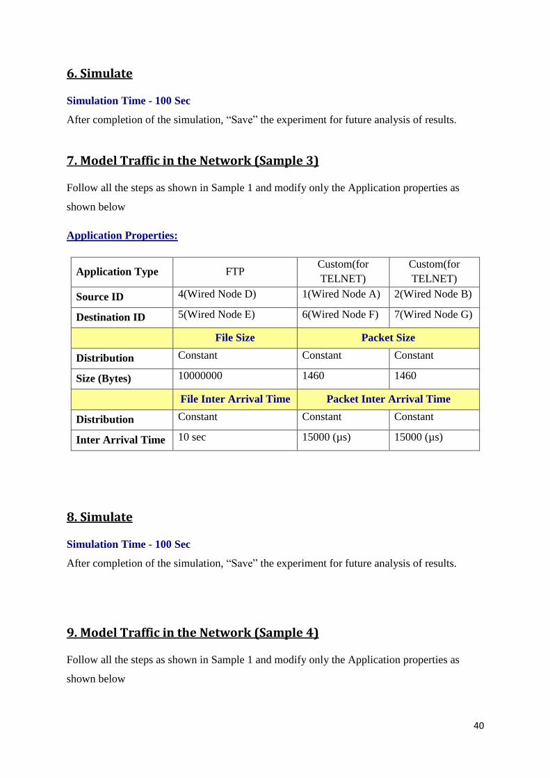
7. Model Traffic in the Network (Sample 3)
Follow all the steps as shown in Sample 1 and modify only the Application properties as
shown below
Application Properties:
Application Type FTP Custom(for
TELNET)
Custom(for
TELNET)
Source ID 4(Wired Node D) 1(Wired Node A) 2(Wired Node B)
Destination ID 5(Wired Node E) 6(Wired Node F) 7(Wired Node G)
File Size Packet Size
Distribution Constant Constant Constant
Size (Bytes) 10000000 1460 1460
File Inter Arrival Time Packet Inter Arrival Time
Distribution Constant Constant Constant
Inter Arrival Time 10 sec 15000 (µs) 15000 (µs)
8. Simulate
Simulation Time - 100 Sec
After completion of the simulation, “Save” the experiment for future analysis of results.
9. Model Traffic in the Network (Sample 4)
Follow all the steps as shown in Sample 1 and modify only the Application properties as
shown below

41
Application Properties:
Application Type FTP Custom(for
TELNET)
Custom(for
TELNET)
Custom(for
TELNET)
Source ID 4(Wired Node D) 1(Wired
Node A)
2(Wired
Node B)
3(Wired
Node C)
Destination ID 5(Wired Node E) 6(Wired
Node F)
7(Wired
Node G)
8(Wired
Node H)
File Size Packet Size
Distribution Constant Constant Constant Constant
Size (Bytes) 10000000 1460 1460 1460
File Inter Arrival
Time
Packet Inter Arrival Time
Distribution Constant Constant Constant Constant
Inter Arrival Time 10 sec 15000 (µs) 15000 (µs) 15000 (µs)
10. Simulate
Simulation Time - 100 Sec
After completion of the simulation, “Save” the experiment for future analysis of results.
11. Analysis of Result
Go to Simulation Open Metrics menu to open the results of saved experiments.
Click on Browse and select the Metrics.txt file (present with the saved experiment) you want
to open

42
Open the Metrics.txt file of the first saved sample and note down the Throughput values
available under Application metrics in the metrics screen of NetSim in an Excel file.
Similarly please follow the same steps for all the saved samples and note down the
Throughput values .It will be as shown below.
Experiment
Number Source Destination Application Throughput
1 Wired Node D Wired Node E FTP 0.824842
2 Wired Node D Wired Node E FTP 0.672768
2 Wired Node A Wired Node F TELNET 0.255091
3 Wired Node D Wired Node E FTP 0.562158
3 Wired Node A Wired Node F TELNET 0.187814
3 Wired Node B Wired Node G TELNET 0.193654
4 Wired Node D Wired Node E FTP 0.487990
4 Wired Node A Wired Node F TELNET 0.149154
4 Wired Node B Wired Node G TELNET 0.146467
4 Wired Node C Wired Node H TELNET 0.156862
Graph I
0
0.1
0.2
0.3
0.4
0.5
0.6
0.7
0.8
0.9
1FTP 1FTP+1Telnet 1FTP+2Telnet 1FTP+3Telnet
FT
P T
hro
ughput
(Mbps)
Experiments
FTP Throughput

43
Graph II
NOTE: The procedure to create graph is same as provided in Experiment 2.
12. Inference
From Graph I, it can be inferred that FTP throughput decreases as the number of transmitting
nodes of TELNET application increases. Wired link 5 is used for FTP traffic. All TELNET
applications in this experiment also used Wired Link 5. Hence as the TELNET traffic over
wired link 5 increases the FTP throughput decreases.
From Graph II, it can be inferred that TELNET throughput of Wired Node 1 decreases as the
number of transmitting nodes of TELNET application increases. TELNET traffic of wired
node 1 flows through wired link 5. Other TELNET applications also used the wired link 5.
Hence as the overall TELNET traffic over wired link 5 increases, the TELNET throughput of
Wired Node 1 decreases.
0
0.05
0.1
0.15
0.2
0.25
0.3
1FTP+1Telnet 1FTP+2Telnet 1FTP+3TelnetTE
LN
ET
Thro
ughput
(Mbps)
of
Wir
ed
Node
1
Experiments
TELNET Throughput of Wired Node 1
44
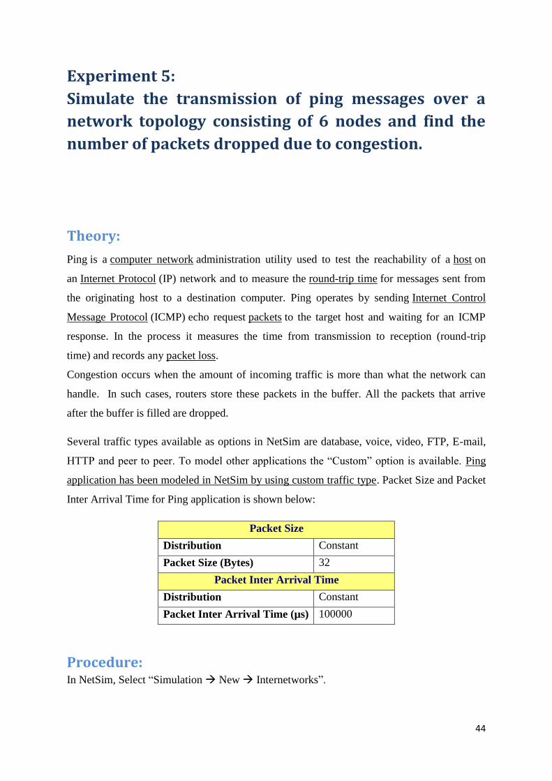
Experiment 5:
Simulate the transmission of ping messages over a
network topology consisting of 6 nodes and find the
number of packets dropped due to congestion.
Theory:
Ping is a computer network administration utility used to test the reachability of a host on
an Internet Protocol (IP) network and to measure the round-trip time for messages sent from
the originating host to a destination computer. Ping operates by sending Internet Control
Message Protocol (ICMP) echo request packets to the target host and waiting for an ICMP
response. In the process it measures the time from transmission to reception (round-trip
time) and records any packet loss.
Congestion occurs when the amount of incoming traffic is more than what the network can
handle. In such cases, routers store these packets in the buffer. All the packets that arrive
after the buffer is filled are dropped.
Several traffic types available as options in NetSim are database, voice, video, FTP, E-mail,
HTTP and peer to peer. To model other applications the “Custom” option is available. Ping
application has been modeled in NetSim by using custom traffic type. Packet Size and Packet
Inter Arrival Time for Ping application is shown below:
Packet Size
Distribution Constant
Packet Size (Bytes) 32
Packet Inter Arrival Time
Distribution Constant
Packet Inter Arrival Time (µs) 100000
Procedure: In NetSim, Select “Simulation New Internetworks”.

45
1. Create /Design the Network
Devices Required: 1 Router, 6 Wired Nodes
Network Diagram:
2. Configure the Network (Sample 1)
Wired Node Properties:
Disable TCP in Wired Node B.
Note: While creating network, place the devices according to the Node ID given in
diagram below in order to easily understand the settings to be configured as provided in
this manual.
For example: Figure shows Wired Node A has Node ID 1 and Wired Node B has Node
ID 2.So first place a Wired Node at the location of Wired Node A and then at Wired
Node B and so on.

46
Right Click Wired Node B Properties
Router Properties: Right click on Router Properties. Set buffer size to 8 MB. Set
scheduling type of interface connected to Wired Node G to FIFO.
Wired Link Properties: Right click on Wired Link Properties and set the values.
Link Properties Wired Link 1 Wired Link 6
Uplink Speed (Mbps) 1.54 0.064
Downlink Speed (Mbps) 1.54 0.064
Uplink BER 10-6
10-6
Downlink BER 10-6
10-6

47
3. Model Traffic in the Network (Sample 1)
Select the Application Button and click on the gap between the Grid Environment and the
ribbon. Now right click on Application and select Properties.
Application Properties:
Application Type Voice Custom
Source ID 2(Wired Node B) 2(Wired Node B)
Destination ID 7(Wired Node G) 7(Wired Node G)
Codec Custom ---
Packet Size
Distribution Constant Constant
Packet Size(Size) 160 32
Packet Inter Arrival Time
Distribution Constant Constant
Packet Inter Arrival
Time (µs) 10000 100000
Service Type CBR ---
NOTE: The procedure to create multiple applications are as follows:
Step 1: Click on the ADD button present in the bottom left corner to add a new application.
4. Simulate
Simulation Time - 100 Sec
After completion of the experiment, “Save” the
experiment for future analysis of results.

48
5. Configure the Network (Sample 2)
Follow all the steps as shown in Sample 1 and modify only the Router properties as shown
below
OR
User can also select the “Go back to Network” option, select the Edit button and modify
only the Router properties as shown below.
Router Properties: Right click on Router Properties. Set buffer size to 8 MB. Set
scheduling type of interface connected to Wired Node G to Priority.
6. Simulate
Simulation Time - 100 Sec
After completion of the experiment, “Save” the experiment for future analysis of results.
7. Configure the Network (Sample 3)
Follow all the steps as shown in Sample 1 and modify only the Router properties and Wired
Link properties as shown below
Router Properties: Right click on Router Properties. Set buffer size to 8 MB. Set
scheduling type of interface connected to Wired Node G to FIFO.

49
Wired Link Properties: Right click on Wired Link Properties and set the values.
Link Properties Wired Link 1 & 2 Wired Link 6
Uplink Speed (Mbps) 1.54 0.064
Downlink Speed (Mbps) 1.54 0.064
Uplink BER 10-6
10-6
Downlink BER 10-6
10-6
8. Model Traffic in the Network (Sample 3)
Select the Application Button and click on the gap between the Grid Environment and the
ribbon. Now right click on Application and select Properties.
Application Properties:
Application Type Voice Voice Custom
Source ID 3(Wired Node C) 2(Wired Node B) 2(Wired Node B)
Destination ID 7(Wired Node G) 7(Wired Node G) 7(Wired Node G)
Codec Custom Custom ---
Packet Size
Distribution Constant Constant Constant
Packet Size(Size) 160 160 32
Packet Inter Arrival Time
Distribution Constant Constant Constant
Packet Inter
Arrival Time (µs) 10000 10000 100000
Service Type CBR CBR ---
50
9. Simulate
Simulation Time - 100 Sec
After completion of the experiment, “Save” the experiment for future analysis of results.
10. Configure the Network (Sample 4)
Follow all the steps as shown in Sample 3 and modify only the Router properties as shown
below
Router Properties: Right click on Router Properties. Set buffer size to 8 MB. Set
scheduling type of interface connected to Wired Node G to Priority.
11. Simulate
Simulation Time - 100 Sec
After completion of the experiment, “Save” the experiment for future analysis of results.
12. Configure the Network (Sample 5)
Follow all the steps as shown in Sample 1 and modify only the Router properties and Wired
Link properties as shown below
Router Properties: Right click on Router Properties. Set buffer size to 8 MB. Set
scheduling type of interface connected to Wired Node G to FIFO.

51
Wired Link Properties: Right click on Wired Link Properties and set the values.
Link Properties Wired Link 1,2 & 3 Wired Link 6
Uplink Speed (Mbps) 1.54 0.064
Downlink Speed (Mbps) 1.54 0.064
Uplink BER 10-6
10-6
Downlink BER 10-6
10-6
13. Model Traffic in the Network (Sample 5)
Select the Application Button and click on the gap between the Grid Environment and the
ribbon. Now right click on Application and select Properties.
Application Properties:
Application Type Voice Voice Voice Custom
Source ID 4(Wired Node
D)
3(Wired Node
C)
2(Wired Node
B)
2(Wired Node
B)
Destination ID 7(Wired Node
G)
7(Wired Node
G)
7(Wired Node
G)
7(Wired Node
G)
Codec Custom Custom Custom ---
Packet Size
Distribution Constant Constant Constant Constant
Packet Size(Size) 160 160 160 32
Packet Inter Arrival Time
Distribution Constant Constant Constant Constant
Packet Inter
Arrival Time (µs) 10000 10000 10000 100000
Service Type CBR CBR CBR ---
14. Simulate
Simulation Time - 100 Sec
After completion of the experiment, “Save” the experiment for future analysis of results.
52
15. Configure the Network (Sample 6)
Follow all the steps as shown in Sample 5 and modify only the Router properties as shown
below
Router Properties: Right click on Router Properties. Set buffer size to 8 MB. Set
scheduling type of interface connected to Wired Node G to Priority.
16. Simulate
Simulation Time - 100 Sec
After completion of the experiment, “Save” the experiment for future analysis of results.
17. Configure the Network (Sample 7)
Follow all the steps as shown in Sample 1 and modify only the Router properties and Wired
Link properties as shown below
Router Properties: Right click on Router Properties. Set buffer size to 8 MB. Set
scheduling type of interface connected to Wired Node G to FIFO.

53
Wired Link Properties: Right click on Wired Link Properties and set the values.
Link Properties Wired Link 1,2,3 & 4 Wired Link 6
Uplink Speed (Mbps) 1.54 0.064
Downlink Speed (Mbps) 1.54 0.064
Uplink BER 10-6
10-6
Downlink BER 10-6
10-6
18. Model Traffic in the Network (Sample 7)
Select the Application Button and click on the gap between the Grid Environment and the
ribbon. Now right click on Application and select Properties.
Application Properties:
Application Type Voice Voice Voice Voice Custom
Source ID 5(Wired
Node E)
4(Wired
Node D)
3(Wired
Node C)
2(Wired
Node B)
2(Wired
Node B)
Destination ID 7(Wired
Node G)
7(Wired
Node G)
7(Wired
Node G)
7(Wired
Node G)
7(Wired
Node G)
Codec Custom Custom Custom Custom ---
Packet Size
Distribution Constant Constant Constant Constant Constant
Packet Size(Size) 160 160 160 160 32
Packet Inter Arrival Time
Distribution Constant Constant Constant Constant Constant
Packet Inter
Arrival Time (µs) 10000 10000 10000 10000 100000
Service Type CBR CBR CBR CBR ---
19. Simulate
Simulation Time - 100 Sec
After completion of the experiment, “Save” the experiment for future analysis of results.

54
20. Configure the Network (Sample 8)
Follow all the steps as shown in Sample 7 and modify only the Router properties as shown
below
Router Properties: Right click on Router Properties. Set buffer size to 8 MB. Set
scheduling type of interface connected to Wired Node G to Priority.
21. Simulate
Simulation Time - 100 Sec
After completion of the experiment, “Save” the experiment for future analysis of results.
22. Configure the Network (Sample 9)
Follow all the steps as shown in Sample 1 and modify only the Router properties and Wired
Link properties as shown below
Router Properties: Right click on Router Properties. Set buffer size to 8 MB. Set
scheduling type of interface connected to Wired Node G to FIFO.

55
Wired Link Properties: Right click on Wired Link Properties and set the values.
Link Properties Wired Link 1,2,3,4 & 5 Wired Link 6
Uplink Speed (Mbps) 1.54 0.064
Downlink Speed (Mbps) 1.54 0.064
Uplink BER 10-6
10-6
Downlink BER 10-6
10-6
23. Model Traffic in the Network (Sample 9)
Select the Application Button and click on the gap between the Grid Environment and the
ribbon. Now right click on Application and select Properties.
Application Properties:
Application Type Voice Voice Voice Voice Voice Custom
Source ID 6(Wired
Node F)
5(Wired
Node E)
4(Wired
Node D)
3(Wired
Node C)
2(Wired
Node B)
2(Wired
Node B)
Destination ID 7(Wired
Node G)
7(Wired
Node G)
7(Wired
Node G)
7(Wired
Node G)
7(Wired
Node G)
7(Wired
Node G)
Codec Custom Custom Custom Custom Custom ---
Packet Size
Distribution Constant Constant Constant Constant Constant Constant
Packet Size(Size) 160 160 160 160 160 32
Packet Inter Arrival Time
Distribution Constant Constant Constant Constant Constant Constant
Packet Inter
Arrival Time (µs) 10000 10000 10000 10000 10000 100000
Service Type CBR CBR CBR CBR CBR ---
24. Simulate
Simulation Time - 100 Sec
After completion of the experiment, “Save” the experiment for future analysis of results.
56
25. Configure the Network (Sample 10)
Follow all the steps as shown in Sample 9 and modify only the Router properties as shown
below
Router Properties: Right click on Router Properties. Set buffer size to 8 MB. Set
scheduling type of interface connected to Wired Node G to Priority.
26. Simulate
Simulation Time - 100 Sec
After completion of the experiment, “Save” the experiment for future analysis of results.
27. Analysis of Result
Go to Simulation Open Metrics menu to open the results of saved experiments.
Click on Browse and select the Metrics.txt file (present with the saved experiment) you want
to open

57
Open the Metrics.txt file of the first sample and note down the total number of Dropped
Packets available under Queue metrics and number of ping messages (Packets Received)
received available under Application metrics in an Excel file. Similarly please follow the
same steps for all the saved samples and note down the dropped packets values .It will be as
shown below.
Sample
Number
No. of voice
applications Scheduling type
Ping messages
received
Total no. of
dropped packets
1 1 FIFO 359 0
2 1 Priority 0 0
3 2 FIFO 183 0
4 2 Priority 0 0
5 3 FIFO 123 0
6 3 Priority 0 0
7 4 FIFO 92 0
8 4 Priority 0 0
9 5 FIFO 74 1896
10 5 Priority 0 1879
28. Inference
From the table we can observe that number of ping messages received when scheduling type
is Priority is less than number of ping messages received when scheduling type is FIFO. In
NetSim, Voice messages have higher priority compared to ping messages. Hence when
scheduling type is Priority, higher preference is given to voice messages. As a result, the
number of ping messages received is lower when priority based scheduling is considered.
From the table we can observe that packets are dropped when there are five voice
applications. The number of packets that arrive at the router increases when there are more
number of voice applications. As a result the buffer gets filled. All the packets that arrive
after the buffer is filled will be dropped.

58
Experiment 6:
Simulate an Ethernet LAN using n nodes (6-10),
change error rate and data rate and compare
throughput.
Part A: To simulate an Ethernet LAN using n nodes (6-10),
change error rate and compare throughput.
Theory:
Bit error rate (BER):
The bit error rate or bit error ratio is the number of bit errors divided by the total number of
transferred bits during a studied time interval i.e.
BER=Bit errors/Total number of bits
For example, a transmission might have a BER of 10-5
, meaning that on average, 1 out of
every of 100,000 bits transmitted exhibits an error. The BER is an indication of how often a
packet or other data unit has to be retransmitted because of an error. Unlike many other forms
of assessment, bit error rate, BER assesses the full end to end performance of a system
including the transmitter, receiver and the medium between the two. In this way, bit error
rate, BER enables the actual performance of a system in operation to be tested.
Packet Error Rate (PER):
The PER is the number of incorrectly received data packets divided by the total number of
received packets. A packet is declared incorrect if at least one bit is erroneous.
Procedure:
In NetSim, Select “Simulation New Internetworks”.

59
1. Create /Design the Network
Devices Required: 2 Switches, 6 Wired Nodes
Network Diagram:
2. Configure the Network (Sample 1)
Wired Node Properties:
Disable TCP in Wired Node A.
Note: While creating network, place the devices according to the Node ID given in
diagram above in order to easily understand the settings to be configured as provided in
this manual.
For example: Figure shows Wired Node A has Node ID 1 and Wired Node B has Node
ID 2.So first place a Wired Node at the location of Wired Node A and then at Wired
Node B and so on.

60
Wired Link Properties: Right click on Wired Link Properties and set the values.
Link Properties Wired
Link 1
Wired
Link 2
Wired
Link 3
Wired
Link 4
Wired
Link 5
Wired
Link 6
Uplink Speed (Mbps) 10 10 10 10 10 10
Downlink Speed (Mbps) 10 10 10 10 10 10
Uplink BER No Error No Error No Error No Error No Error No Error
Downlink BER No Error No Error No Error No Error No Error No Error
3. Model Traffic in the Network (Sample 1)
Select the Application Button and click on the gap between the Grid Environment and the
ribbon. Now right click on Application and select Properties.
Application Properties:
Application Type Custom
Source ID 1 (Wired Node A)
Destination ID 4 (Wired Node D)
Packet Size
Distribution Constant
Size (Bytes) 1460
Packet Inter Arrival Time
Distribution Constant
Inter Arrival Time 2500
4. Simulate(Sample 1)
Go to IP and ARP configuration and disable static ARP.
61
Simulation Time - 100 Sec
After completion of the experiment, “Save” the experiment for future analysis of results.
5. Configure the Network (Sample 2)
Follow all the steps as shown in Sample 1 and modify only the Wired Link properties as
shown below.
OR
User can also select the “Go back to Network” option, select the Edit button and modify
only the wired link properties as shown below.
Wired Link Properties: Right click on Wired Link Properties and set the values.
Link Properties Wired
Link 1
Wired
Link 2
Wired
Link 3
Wired
Link 4
Wired
Link 5
Wired
Link 6
Uplink Speed (Mbps) 10 10 10 10 10 10
Downlink Speed (Mbps) 10 10 10 10 10 10
Uplink BER 10-9
10-9 10
-9 10-9 10
-9 10-9
Downlink BER 10-9 10
-9 10-9 10
-9 10-9 10
-9

62
6. Simulate
Go to IP and ARP configuration and disable static ARP.
Simulation Time - 100 Sec
After completion of the experiment, “Save” the experiment for future analysis of results.
7. Configure the Network (Sample 3)
Follow all the steps as shown in Sample 1 and modify only the Wired Link properties as
shown below
Wired Link Properties: Right click on Wired Link Properties and set the values.
Link Properties Wired
Link 1
Wired
Link 2
Wired
Link 3
Wired
Link 4
Wired
Link 5
Wired
Link 6
Uplink Speed (Mbps) 10 10 10 10 10 10
Downlink Speed (Mbps) 10 10 10 10 10 10
Uplink BER 10-8 10
-8 10-8 10
-8 10-8 10
-8
Downlink BER 10-8 10
-8 10-8 10
-8 10-8 10
-8
8. Simulate
Go to IP and ARP configuration and disable static ARP.
Simulation Time - 100 Sec
After completion of the experiment, “Save” the experiment for future analysis of results.
9. Configure the Network (Sample 4)
Follow all the steps as shown in Sample 1 and modify only the Wired Link properties as
shown below
Wired Link Properties: Right click on Wired Link Properties and set the values.
Link Properties Wired
Link 1
Wired
Link 2
Wired
Link 3
Wired
Link 4
Wired
Link 5
Wired
Link 6
Uplink Speed (Mbps) 10 10 10 10 10 10
Downlink Speed (Mbps) 10 10 10 10 10 10
Uplink BER 10-7 10
-7 10-7 10
-7 10-7 10
-7
Downlink BER 10-7 10
-7 10-7 10
-7 10-7 10
-7

63
10. Simulate
Go to IP and ARP configuration and disable static ARP.
Simulation Time - 100 Sec
After completion of the experiment, “Save” the experiment for future analysis of results.
11. Configure the Network (Sample 5)
Follow all the steps as shown in Sample 1 and modify only the Wired Link properties as
shown below
Wired Link Properties: Right click on Wired Link Properties and set the values.
Link Properties Wired
Link 1
Wired
Link 2
Wired
Link 3
Wired
Link 4
Wired
Link 5
Wired
Link 6
Uplink Speed (Mbps) 10 10 10 10 10 10
Downlink Speed (Mbps) 10 10 10 10 10 10
Uplink BER 10-6 10
-6 10-6 10
-6 10-6 10
-6
Downlink BER 10-6 10
-6 10-6 10
-6 10-6 10
-6
12. Simulate
Go to IP and ARP configuration and disable static ARP.
Simulation Time - 100 Sec
After completion of the experiment, “Save” the experiment for future analysis of results.
13. Analysis of Result
Go to NetSim Analytics(Simulation Analytics).
1. Click Browse button select the Metrics.txt File inside the first saved
experiment folder
2. Add the remaining 5 sample experiments by repeating the above step.
3. Select the Metrics - Select the coordinates for Y-axis by clicking on the
dropdown menu. User should select “Packets Errored”.

64
Comparison Chart:
Graph I: Error Rate Vs Packets Errored
Go to Simulation Open Metrics menu to open the results of saved experiments.
Click on Browse and select the Metrics.txt file (present with the saved experiment) you want
to open
Open the Metrics.txt file of the first saved sample and note down the “Throughput” value
available under “Application Metrics” in an Excel file. Similarly please follow the same
steps for all the saved samples and note down the throughput values and create graph in Excel
as shown below.

65
Graph II: Error Rate Vs Throughput
NOTE: The procedure to create graph is same as provided in Experiment 2.
Part B: To simulate an Ethernet LAN using n nodes (6-10),
change data rate and compare throughput.
Theory:
Data Rate:
Data Rate is the speed at which data can be transmitted from one device to another. It is often
measured in megabits (million bits) per second.
Procedure:
In NetSim, Select “Simulation New Internetworks”.
1. Create /Design the Network
Devices Required: 2 Switches, 6 Wired Nodes
4.4
4.45
4.5
4.55
4.6
4.65
4.7
No Error 10^-9 10^-8 10^-7 10^-6
Thro
ughput
Error Rate
Error Rate vs Throughput

66
Network Diagram:
2. Configure the Network (Sample 1)
Wired Node Properties:
Disable TCP in Wired Node A.
Note: While creating network, place the devices according to the Node ID given in
diagram above in order to easily understand the settings to be configured as provided in
this manual.
For example: Figure shows Wired Node A has Node ID 1 and Wired Node B has Node
ID 2.So first place a Wired Node at the location of Wired Node A and then at Wired
Node B and so on.

67
Wired Link Properties: Right click on Wired Link Properties and set the values.
Link Properties Wired
Link 1
Wired
Link 4
Wired
Link 6
Uplink Speed (Mbps) 20 20 20
Downlink Speed (Mbps) 20 20 20
Uplink BER No Error No Error No Error
Downlink BER No Error No Error No Error
3. Model Traffic in the Network (Sample 1)
Select the Application Button and click on the gap between the Grid Environment and the
ribbon. Now right click on Application and select Properties.
Application Properties:
Application Type Custom
Source ID 1 (Wired Node A)
Destination ID 4 (Wired Node D)
Packet Size
Distribution Constant
Size (Bytes) 10000
Packet Inter Arrival Time
Distribution Constant
Inter Arrival Time 1000
4. Simulate
Simulation Time - 10 Sec
After completion of the experiment, “Save” the experiment for future analysis of results.
5. Configure the Network (Sample 2)
Follow all the steps as shown in Sample 1 and modify only the Wired Link properties as
shown below
OR

68
User can also select the “Go back to Network” option, select the Edit button and modify
only the wired link properties as shown below.
Wired Link Properties: Right click on Wired Link Properties and set the values.
Link Properties Wired
Link 1
Wired
Link 4
Wired
Link 6
Uplink Speed (Mbps) 40 40 40
Downlink Speed (Mbps) 40 40 40
Uplink BER No Error No Error No Error
Downlink BER No Error No Error No Error
6. Simulate
Simulation Time – 10 Sec
After completion of the experiment, “Save” the experiment for future analysis of results.
7. Configure the Network (Sample 3)
Follow all the steps as shown in Sample 1 and modify only the Wired Link properties as
shown below
Wired Link Properties: Right click on Wired Link Properties and set the values.
Link Properties Wired
Link 1
Wired
Link 4
Wired
Link 6
Uplink Speed (Mbps) 60 60 60
Downlink Speed (Mbps) 60 60 60
Uplink BER No Error No Error No Error
Downlink BER No Error No Error No Error
8. Simulate
Simulation Time - 10 Sec
After completion of the experiment, “Save” the experiment for future analysis of results.

69
9. Configure the Network (Sample 4)
Follow all the steps as shown in Sample 1 and modify only the Wired Link properties as
shown below
Wired Link Properties: Right click on Wired Link Properties and set the values.
Link Properties Wired
Link 1
Wired
Link 4
Wired
Link 6
Uplink Speed (Mbps) 80 80 80
Downlink Speed (Mbps) 80 80 80
Uplink BER No Error No Error No Error
Downlink BER No Error No Error No Error
10. Simulate
Simulation Time - 10 Sec
After completion of the experiment, “Save” the experiment for future analysis of results.
11. Analysis of Result
Go to Simulation Open Metrics menu to open the results of saved experiments.
Click on Browse and select the Metrics.txt file (present with the saved experiment) you want
to open

70
Open the Metrics.txt file of the first sample and note down the “Throughput” value
available under “Application Metrics” in an Excel file. Similarly please follow the same
steps for all the saved samples, note down the throughput values and create Graph in Excel as
shown below.
Graph I
Data Rate Vs Throughput
NOTE: The procedure to create graph is same as provided in Experiment 2.
12. Inference
The number of packets transmitted to the destination is based on the network link‟s speed. So
when link is forwarding more packets, the number of packets transmitted to the destination is
more. Because of this throughput linearly increases when data rate (link speed) increases in
Graph I.
0
10
20
30
40
50
60
70
80
20 40 60 80
Thro
ughput
Data Rate
Data Rate Vs Throughput

71
Experiment 7:
To Simulate an Ethernet LAN using n nodes and set
multiple traffic nodes and determine collision across
different nodes.
Theory:
Carrier Sense Multiple Access Collision Detection (CSMA / CD)
This protocol includes the improvements for stations to abort their transmissions as soon as
they detect a collision. Quickly terminating damaged frames saves time and bandwidth. This
protocol is widely used on LANs in the MAC sub layer. If two or more stations decide to
transmit simultaneously, there will be a collision. Collisions can be detected by looking at the
power or pulse width of the received signal and comparing it to the transmitted signal. After a
station detects a collision, it aborts its transmission, waits a random period of time and then
tries again, assuming that no other station has started transmitting in the meantime.
Procedure:
In NetSim, Select “Simulation New Legacy Networks Traditional Ethernet”.
1. Create /Design the Network
Devices Required: 1 Hub, 5 Wired Nodes
Network Diagram:
Note: While creating network, first
place the Hub. Then select Wired
Node and click on Hub.
Automatically Wired Nodes will be
placed and linked with Hub.
72
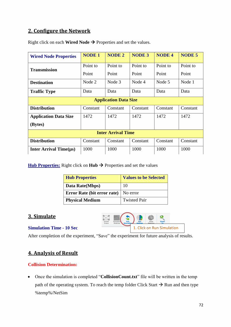
2. Configure the Network
Right click on each Wired Node Properties and set the values.
Hub Properties: Right click on Hub Properties and set the values
Hub Properties Values to be Selected
Data Rate(Mbps) 10
Error Rate (bit error rate) No error
Physical Medium Twisted Pair
3. Simulate
Simulation Time - 10 Sec
After completion of the experiment, “Save” the experiment for future analysis of results.
4. Analysis of Result
Collision Determination:
Once the simulation is completed “CollisionCount.txt” file will be written in the temp
path of the operating system. To reach the temp folder Click Start Run and then type
%temp%/NetSim
Wired Node Properties NODE 1 NODE 2 NODE 3 NODE 4 NODE 5
Transmission Point to
Point
Point to
Point
Point to
Point
Point to
Point
Point to
Point
Destination Node 2 Node 3 Node 4 Node 5 Node 1
Traffic Type Data Data Data Data Data
Application Data Size
Distribution Constant Constant Constant Constant Constant
Application Data Size
(Bytes)
1472 1472 1472 1472 1472
Inter Arrival Time
Distribution Constant Constant Constant Constant Constant
Inter Arrival Time(µs) 1000 1000 1000 1000 1000

73
Open the file in Excel
Comparison Table:
If collision occurs, the entry will be added in the table by incrementing the “Collision
_Count” field value by 1. So the last entry of the particular “Source_ID” will consist of
“Total Collision_Count”.
74
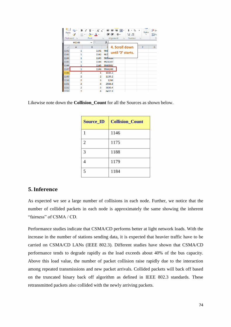
Likewise note down the Collision_Count for all the Sources as shown below.
Source_ID Collision_Count
1 1146
2 1175
3 1188
4 1179
5 1184
5. Inference
As expected we see a large number of collisions in each node. Further, we notice that the
number of collided packets in each node is approximately the same showing the inherent
“fairness” of CSMA / CD.
Performance studies indicate that CSMA/CD performs better at light network loads. With the
increase in the number of stations sending data, it is expected that heavier traffic have to be
carried on CSMA/CD LANs (IEEE 802.3). Different studies have shown that CSMA/CD
performance tends to degrade rapidly as the load exceeds about 40% of the bus capacity.
Above this load value, the number of packet collision raise rapidly due to the interaction
among repeated transmissions and new packet arrivals. Collided packets will back off based
on the truncated binary back off algorithm as defined in IEEE 802.3 standards. These
retransmitted packets also collided with the newly arriving packets.

75
Experiment 8:
To Simulate an Ethernet LAN using n nodes and set
multiple traffic nodes and plot contention window for
different source/destination.
Theory:
Carrier Sense Multiple Access Collision Detection (CSMA/CD) - Working of the
truncated binary back off algorithm
In Ethernet networks, the CSMA/CD is commonly used to schedule retransmissions after
collisions. The retransmission is delayed by an amount of time derived from the slot time and
the number of attempts to retransmit.
After c collisions, a random number of slot times between 0 and 2c - 1 is chosen. For the first
collision, each sender will wait 0 or 1 slot times. After the second collision, the senders will
wait anywhere from 0 to 3 slot times (inclusive). After the third collision, the senders will
wait anywhere from 0 to 7 slot times (inclusive), and so forth. As the number of
retransmission attempts increases, the number of possibilities for delay increases
exponentially.
The 'truncated' simply means that after a certain number of increases, the exponentiation
stops; i.e. the retransmission timeout reaches a ceiling, and thereafter does not increase any
further. For example, if the ceiling is set at i = 10 (as it is in the IEEE 802.3 CSMA/CD
standard), then the maximum delay is 1023 slot times.
Because these delays cause other stations that are sending to collide as well, there is a possibility
that, on a busy network, hundreds of people may be caught in a single collision set. Because of this
possibility, after 16 attempts at transmission, the process is aborted.
Procedure:
In NetSim, Select “Simulation New Legacy Networks Traditional Ethernet”.

76
1. Create /Design the Network
Devices Required: 1 Hub, 4 Wired Nodes
Network Diagram:
2. Configure the Network
Right click on Wired Node or Hub and select Properties to open the property window.
Wired Node Properties:
Hub Properties:
Hub Properties Values to be Selected
Data Rate(Mbps) 10
Error Rate (bit error rate) No error
Physical Medium Twisted Pair
Wired Node Properties NODE 1 NODE 4
Transmission Type Point to Point Point to Point
Destination Node 2 Node 1
Traffic Type Data Data
Application Data Size
Distribution Constant Constant
Application Data Size (Bytes) 1472 1472
Inter Arrival Time
Distribution Constant Constant
Inter Arrival Time(µs) 2000 2000
Note: While creating network,
first place the Hub. Then select
Wired Node and click on Hub.
Automatically Wired Nodes will
be placed and linked with Hub.

77
3. Simulate
Simulation Time - 10 Sec
4. Analysis of Result
Once the simulation is completed “ContentionWindow.txt” file will be written in the
temp path of the operating system. To reach the temp folder, Click Start Run or press
(Windows Key) + R and then type “%temp%/NetSim”.
Open the file in Excel.
Comparison Chart:
Graph I
(Note: These charts are plotted only for Source_ID 1. The procedure is as follows)

78
Time vs. Contention Window Size Graph
(Note: This graph is plotted for all rows of ContentionWindow.txt file after filtering, X-Axis
is Contention_Window column and Y-Axis is Time(Micro Sec) column.)
NOTE: The procedure to create graph is same as provided in Experiment 2.
-200
0
200
400
600
800
1000
1200
0 2000000 4000000 6000000 8000000 10000000 12000000
Co
nte
nti
on
Win
do
w S
ize
(Byt
e)
Time (Micro Secs)
Time Vs. Contention Window Size

79
Graph II
(Note: This graph is plotted for the first 200 rows of ContentionWindow.txt file, X-Axis is
Contention_Window column and Y-Axis is Time(Micro Sec) column.)
Time vs. Contention Window Size Graph
NOTE: The procedure to create graph is same as provided in Experiment 2.
5. Inference
As explained above in the theory part, whenever a collision occurs the contention window
size is calculated and a random number is generated. With more number of transmitting
nodes, the contention for the medium increases, causing more collisions and more
retransmission attempts. Hence the average contention window increases.
From the above graph it can be observed that, for each collision the contention window size
increases, and at any time the maximum contention window size is 1023 (210
-1). The
maximum retry limit for a packet is 16, after which the packet is dropped.
-200
0
200
400
600
800
1000
1200
0 500000 1000000 1500000 2000000
Co
nte
nti
on
Win
do
w S
ize
(Byt
e)
Time (Micro Secs)
Time Vs. Contention Window Size

80
Experiment 9:
To simulate simple ESS and with transmitting nodes in
wireless LAN by simulation and determine the
performance with respect to transmission of packets.
Theory:
Wireless LAN is basically a LAN that transmits data over air, without any physical
connection between devices. The transmission medium is a form of electromagnetic
radiation. Wireless LAN is ratified by IEEE in the IEEE 802.11 standard. In most of the
WLAN products on the market based on the IEEE 802.11b technology the transmitter is
designed as a Direct Sequence Spread Spectrum Phase Shift Keying (DSSS PSK) modulator,
which is capable of handling data rates of up to 11 Mbps. The underlying algorithm used in
Wireless LAN is known as the CSMA/CA – Carrier Sense Multiple Access/Collision
Avoidance algorithm.
Procedure:
In NetSim, Select “Simulation New Internetworks”.
1. Create /Design the Network
Devices Required: 1 Switch, 2 Access Point, 6 Wireless Nodes.
Device Placement:
NOTE: To edit the position, change the (x, y) co-ordinates in Global Properties as
shown:
To change
Co-ordinates,
click & edit

81
Set the exact x and y co-ordinates for respective device in device property which is
mentioned in the above table to get the same result as obtained in this manual.
Device Name X /Lat Y /Lon
Access Point A 170 110
Access Point B 331 191
Switch C 251 151
Wireless Node D 130 110
Wireless Node E 145 87
Wireless Node F 170 70
Wireless Node G 331 230
Wireless Node H 360 220
Wireless Node I 371 190
Network Diagram:
2. Configure the Network (Sample 1)
Wired Node Properties:
Disable TCP in Wireless Node D.
Right Click Wireless Node D Properties

82
3. Model Traffic in the Network (Sample 1)
Select the Application Button and click on the gap between the Grid Environment and the
ribbon. Now right click on Application and select Properties.
Application Properties:
4. Simulate(Sample 1)
Simulation Time - 10 Sec
After completion of the experiment, “Save”
the experiment for future analysis of
results.
Application Type Custom
Source ID 4(Wireless Node D)
Destination ID 7(Wireless Node G)
Packet Size
Distribution Constant
Value(Bytes) 1460
Inter Arrival Time
Distribution Constant
Value(µs) 2336

83
5. Configure the Network (Sample 2)
Follow all the steps as shown in Sample 1 and modify only the Wired Node properties and
Application properties as shown below
OR
User can also select the “Go back to Network” option, select the Edit button and modify
only the Wired Node properties and Application properties as shown below.
Wired Node Properties:
Disable TCP in Wireless Node D and Wireless Node E.
All the remaining properties of the remaining devices and links are same.
6. Model Traffic in the Network (Sample 2)
Application Properties:
7. Simulate(Sample 2)
Simulation Time - 10 Sec
After completion of the simulation, “Save” the experiment for future analysis of results.
Application Type Custom Custom
Source ID 4(Wireless Node D) 5(Wireless Node E)
Destination ID 7(Wireless Node G) 8(Wireless Node H)
Packet Size
Distribution Constant Constant
Value(Bytes) 1460 1460
Inter Arrival Time
Distribution Constant Constant
Value(µs) 2336 2336

84
8. Configure the Network (Sample 3)
Follow all the steps as shown in Sample 1 and modify only the Wired Node properties and
Application properties as shown below
Wired Node Properties:
Disable TCP in Wireless Node D, Wireless Node E and Wireless Node F.
All the remaining properties of the remaining devices and links are same.
9. Model Traffic in the Network (Sample 3)
Application Properties:
10. Simulate(Sample 3)
Simulation Time - 10 Sec
After completion of the simulation, “Save” the experiment for future analysis of results.
11. Configure the Network (Sample 4)
Follow all the steps as shown in Sample 1 and modify only the Wired Node properties and
Application properties as shown below
Wired Node Properties:
Disable TCP in Wireless Node D, Wireless Node E, Wireless Node F and Wireless Node G.
Application Type Custom Custom Custom
Source ID 4(Wireless Node D) 5(Wireless Node E) 6(Wireless Node F)
Destination ID 7(Wireless Node G) 8(Wireless Node H) 9(Wireless Node I)
Packet Size
Distribution Constant Constant Constant
Value(Bytes) 1460 1460 1460
Inter Arrival Time
Distribution Constant Constant Constant
Value(µs) 2336 2336 2336
85
All the remaining properties of the remaining devices and links are same.
12. Model Traffic in the Network (Sample 4)
Application Properties:
13. Simulate(Sample 4)
Simulation Time - 10 Sec
After completion of the simulation, “Save” the experiment for future analysis of results.
14. Analysis of Result
Go to NetSim Analytics (Simulation Analytics).
1. Click Browse button select the Metrics.txt File inside the first saved
experiment folder
2. Add the remaining 5 sample experiments by repeating the above step.
3. Select the Metrics - Select the coordinates for Y-axis by clicking on the
dropdown menu. User should select “Packets Collided”.
Application Type Custom Custom Custom Custom
Source ID 4(Wireless
Node D)
5(Wireless
Node E)
6(Wireless
Node F)
7(Wireless
Node G)
Destination ID 7(Wireless
Node G)
8(Wireless
Node H)
9(Wireless
Node I)
6(Wireless
Node F)
Packet Size
Distribution Constant Constant Constant Constant
Value(Bytes) 1460 1460 1460 1460
Inter Arrival Time
Distribution Constant Constant Constant Constant
Value(µs) 2336 2336 2336 2336

86
Comparison Chart:
Graph I: Number of nodes generating traffic vs. Packets collided
Go to Simulation Open Metrics menu to open the results of saved experiments.
Click on Browse and select the Metrics.txt file (present with the saved experiment) you want
to open
Open the Metrics.txt file of the first sample and note down the “Throughput” value
available under “Application Metrics” in an Excel file. Similarly please follow the same
steps for all the saved samples, note down the throughput values and create graph in Excel as
shown below.
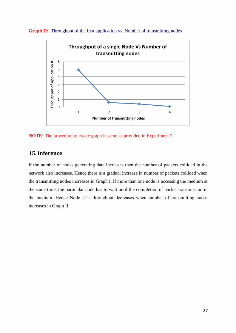
87
Graph II: Throughput of the first application vs. Number of transmitting nodes
NOTE: The procedure to create graph is same as provided in Experiment 2.
15. Inference
If the number of nodes generating data increases then the number of packets collided in the
network also increases. Hence there is a gradual increase in number of packets collided when
the transmitting nodes increases in Graph I. If more than one node is accessing the medium at
the same time, the particular node has to wait until the completion of packet transmission in
the medium. Hence Node #1‟s throughput decreases when number of transmitting nodes
increases in Graph II.
0
1
2
3
4
5
6
1 2 3 4
Thro
ugh
pu
t o
f A
pp
licat
ion
# 1
Number of transmitting nodes
Throughput of a single Node Vs Number of transmitting nodes

88
Experiment 10: Cyclic Redundancy Check
Write a program for error detecting code using CRC-
CCITT (16- bits). (Note: CRC 12, CRC 16 and CRC 32 are
also available in NetSim)
Theory:
Cyclic redundancy check (CRC) is a type of function that takes a data stream of any length as
input, and produces an output. Bit strings are treated as representation of polynomials with
coefficients of „0‟ and „1‟.
The Sender and Receiver must agree upon the Generator Polynomial in advance. Both the
high and low order of the generator must be „1‟. The size of data must be greater than the size
of the Generator polynomial to compute the checksum.
The computed checksum is appended to the transmitting frame. If the receiver gets the frame
it tries dividing it by Generator polynomial, if there is a reminder there has been a
transmission error, else no error.
The Generator polynomial for CRC CCITT is given below,
x16
+x12
+x5+1
The Binary equivalent of CRC - CCITT is 10001000000100001
Algorithm:
No Error Case
Sender side
Get the input from "Input.txt". Parse the file content.

89
Call the In-built function readFile (szfilename). It returns the stored value to the local
variable „szcrc‟.
Convert the data string (szcrc) that has to be transmitted into a binary representation.
1. Get ASCII value of the first character.
2. Divide the ASCII value by 2 and append the remainder to a string. The
quotient is taken as the next number for the division.
3. Repeat the above division until the quotient of the number is less than 2.
4. Finally a remainder string having 1‟s and 0‟s is obtained. This reminder is the
binary representation of that character.
5. Continue the above process for all the characters in the data string (szcrc).
Append 16 „0‟s to the final binary string formed by the above step.
Divide the binary converted data string using the Generator Polynomial (as given
above in Concept).
1. Take the MSB 17 bits from the binary data string,
2. If the leading bit of the binary data string is „0‟, do an XOR operation with the
17 bits of „0‟s and get the remainder which is also 17 bits.
3. Else, if the leading bit of the binary data string is „1‟, do an XOR operation
with the 17 bits with binary converted CRC - CCITT polynomial and get the
remainder which is also 17 bits.
4. The first bit of the remainder is left out and the remainder is made to 16 bits.
5. If there are successive bits in the data, make the previous remainder bit to 17
bits by bringing down the next bit into the data
Convert the final remainder into HEXA equivalent character.
1. Divide the final remainder at the end of step 5.4 into blocks of 4 bits.
2. Convert each block into equivalent HEXA character.
3. Thus the output of this whole process will be a 4 - nibble checksum that is
attached to the transmitting frame.

90
Receiver side CRC Coding
Repeat the Steps 1 to 4 of the Sender side CRC coding and get the „szcrc ‟ value for
the data.
Convert the HEXA equivalent string „szSender‟ to its binary format. This is the
Hexadecimal to binary conversion process.
Append the binary format of the above step to the „szcrc ‟ variable. Then append 16
„0s‟ to the „szcrc ‟ variable.
Repeat the Steps 5 and 6 of the Sender Side CRC coding to calculate the CRC value
for the receiver side. The output is stored in the variable „szReceive‟ (array of
characters with size 10).
Error Case
Sender side
Get the input from "Input.txt". Parse the file content.
Call the In-built function readFile (szfilename). It returns the stored value to the local
variable „szcrc ‟.
Convert the data string (szcrc ) to be transmitted into binary representation.
1. Get ASCII value of the first character.
2. Divide the ASCII value by 2 and append the remainder to a string. The
quotient is taken as the next number for the division.
3. Repeat the above division until the quotient of the number is less than 2.
4. Finally we get the remainder string having 1‟s and 0‟s, which is the binary
representation of that character.
5. Continue above process for all the characters in the data string (szcrc ).
Append 16 „0‟s to the final binary string formed by the above step.
Divide the binary converted data string using the Generator Polynomial (as given
above in Concept).
1. Take the MSB 17 bits from the binary data string,

91
2. If the leading bit of the binary data string is „0‟, do an XOR operation with the
17 bits of „0‟s and get the remainder which is also 17 bits.
3. Else if the leading bit of the binary data string is „1‟, do an XOR operation
with the 17 bits with binary converted CRC - CCITT polynomial and get the
remainder which is also 17 bits.
4. The first bit of the remainder is left out and the remainder is made to 16 bits.
5. If there are successive bits in the data, make the previous remainder bit to 17
bits by bringing down the next bit in the data
Convert the final remainder into HEXA equivalent character.
1. Divide the final remainder at the end of step 5.4 into blocks of 4 bits.
2. Convert each block into equivalent HEXA character.
3. Thus the output of this whole process will be a 4-nibble checksum that is
attached to the transmitting frame.
Receiver side
Repeat the Steps 1 to 4 of the Sender side CRC coding and get the „szcrc ‟ value for
the data.
Make some errors in the string „szcrc ‟ by changing certain characters. The error
string is stored in the variable „szcrc ‟.
Write the Error string „szcrc ‟ into the file „Input.txt‟. The file path for the file
„Input.txt" is the path where you have installed the
NetSim application. (Compulsory).
Convert the HEXA equivalent string „szSender‟ to its binary format. This is the
Hexadecimal to binary conversion process.
Append the binary format of the above step to the „szcrc ‟ variable. Then append 16
„0s‟ to the „szcrc ‟ variable.
Repeat the Steps 5 and 6 of the Sender Side CRC coding to calculate the CRC value
for the receiver side.

92
Procedure:
To begin with the experiment, open NetSim.Click on Programming in the menu bar, select
Error Detecting Codes and then select Cyclic Redundancy Check.
The scenario will be obtained as shown below. Follow the steps.
Step 1:
Select the User mode to write your own program in C/C++, compile and link to NetSim
software for validation. Click on the F1(Help) for details on how to proceed with your own
code.
The scenario will be obtained as shown below. Follow the steps.
Select Mode
Select any of the algorithms
Select Error condition
Click here to add the input
text file
Click here to view concept,
algorithm, pseudo Code &
flow chart
Click
Run to
execute
Click here to interface
source code
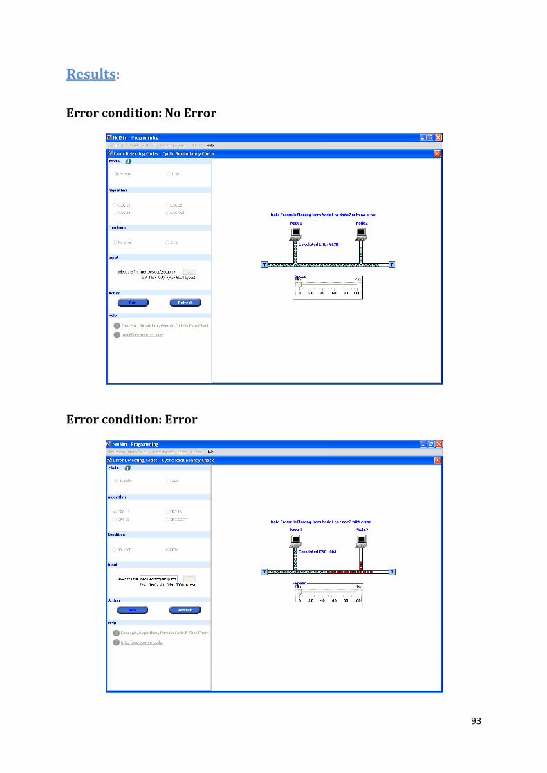
93
Results:
Error condition: No Error
Error condition: Error
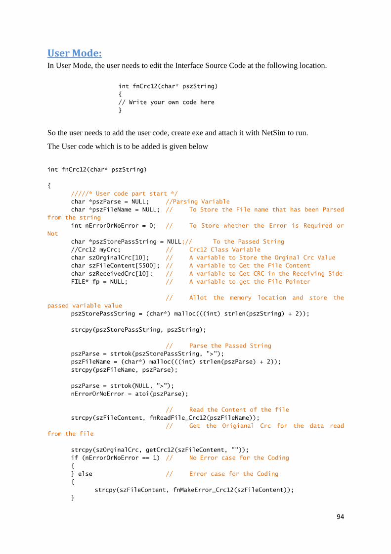
94
User Mode: In User Mode, the user needs to edit the Interface Source Code at the following location.
int fnCrc12(char* pszString)
{
// Write your own code here
}
So the user needs to add the user code, create exe and attach it with NetSim to run.
The User code which is to be added is given below
int fnCrc12(char* pszString)
{
/////* User code part start */
char *pszParse = NULL; //Parsing Variable
char *pszFileName = NULL; // To Store the File name that has been Parsed
from the string
int nErrorOrNoError = 0; // To Store whether the Error is Required or
Not
char *pszStorePassString = NULL;// To the Passed String
//Crc12 myCrc; // Crc12 Class Variable
char szOrginalCrc[10]; // A variable to Store the Orginal Crc Value
char szFileContent[5500]; // A variable to Get the File Content
char szReceivedCrc[10]; // A variable to Get CRC in the Receiving Side
FILE* fp = NULL; // A variable to get the File Pointer
// Allot the memory location and store the
passed variable value
pszStorePassString = (char*) malloc(((int) strlen(pszString) + 2));
strcpy(pszStorePassString, pszString);
// Parse the Passed String
pszParse = strtok(pszStorePassString, ">");
pszFileName = (char*) malloc(((int) strlen(pszParse) + 2));
strcpy(pszFileName, pszParse);
pszParse = strtok(NULL, ">");
nErrorOrNoError = atoi(pszParse);
// Read the Content of the file
strcpy(szFileContent, fnReadFile_Crc12(pszFileName));
// Get the Origianal Crc for the data read
from the file
strcpy(szOrginalCrc, getCrc12(szFileContent, ""));
if (nErrorOrNoError == 1) // No Error case for the Coding
{
} else // Error case for the Coding
{
strcpy(szFileContent, fnMakeError_Crc12(szFileContent));
}

95
// Get the Received Crc for the string
strcpy(szReceivedCrc, getCrc12(szFileContent, szOrginalCrc));
// Make the Output to the Output file
strcpy(szPath_Crc12, szPath1_Crc12);
#ifndef _NETSIMDLL
strcat(szPath_Crc12, "/Output.txt");
#else
strcat(szPath_Crc12, "/Temp.txt");
#endif
// Open the File for Writing
szOutput_path_Crc12 = (char *) malloc(200 * sizeof(char));
strcpy(szOutput_path_Crc12, szTempPath_Crc12);
#ifndef _NETSIMDLL
strcat(szOutput_path_Crc12, "/Output.txt");
#else
strcat(szOutput_path_Crc12, "/Temp.txt");
#endif
fp = fopen(szOutput_path_Crc12, "w");
fprintf(fp, "%s\n%s\n", szOrginalCrc, szReceivedCrc);
fclose(fp);
//delete [] pszStorePassString;
//delete [] pszFileName;
free(pszStorePassString);
free(pszFileName);
/////* User code part end */
return 1;
}
Note- How to practice this experiment without using NetSim:
Users who do not have a licensed version of NetSim in their PC's, can practice as explained
below.
First, run the exercise in sample mode. The user would see that an Input.txt file is created in
Win OS temp folder (this can be reached by typing %temp%/NetSim in Windows run
window). This input file should be read by the user code and it should generate an Output.txt.
This Output.txt file is read by NetSim and shown graphically to the user.
User can follow the steps provided in Appendix 1: Programming exercise - How to practice
without NetSim.
Given below are sample Input.txt and Output.txt files for this experiment for users to verify
& validate their code. The Output.txt file will vary based on the Data_file. In this case, the
Data_File file contains the text “a”.

96
Input.txt file contents
Algorithm=CRC_12
Condition=No_Error
File_Path=C:\Users\TETCOS\Desktop\New Text Document.txt>
*Note- Create any file of size <5000 Byte. Type the location of the file in Data_File.
Output.txt file contents
BCF
000
*Note- Output.txt content will vary depending on the file contents.

97
Experiment 11: Sorting (Bubble Sort)
Write a program for frame sorting technique used in
buffers.
Theory:
Sorting is the ordering of data in either an increasing or decreasing order. One of the
fundamental challenges of computer science is ordering a list of items. Sorting algorithms are
designed with the following objectives:
1. Minimize exchange or wholesale movement of data.
2. Move data from secondary storage to main memory in large blocks. This is done
because larger the data blocks, more the efficiency of the algorithm. This is a key part
of external sorting.
3. If possible, retain all the data in main memory. In this case, random access into an
array can be effectively used. This is a key part in internal sorting.
There are three important considerations that will affect a programmer‟s decision to choose
from a variety of sorting methods.
1. Time to write the program.
2. Execution time of the program.
3. Memory or auxiliary space needed for the program‟s environment.
In this exercise, we will look at the “Bubble” sort algorithm.
By selecting „Sample‟ option, user can visualize the sorting for the given input data and
understand the concept of Sorting.
Algorithm:
Bubble sort derives its name from the fact that the smallest data item bubbles up to the top of
the sorted array.

98
The algorithm begins by comparing the top item of the array with the next, and swapping
them if necessary. After n – 1 comparisons, the largest among a total of n items descends to
the bottom of the array, to the nth location.
The process is then reapplied to the remaining n – 1 items of the array. For n data items, the method
requires n (n – 1)/2 comparisons and, on the average, almost one-half as many swaps. The bubble
sort, therefore, is inefficient in large sorting jobs.
Procedure: To begin with the experiment, open NetSim
Click on Programming in the menu bar, select Sorting Techniques and then select Bubble.
The scenario will be obtained as shown below. Follow the steps.
Step 1:
Select the User mode to write your own program in C/C++, compile and link to NetSim
software for validation. Click on the F1(Help) for details on how to proceed with your own
code.
The scenario will be obtained as shown below. Follow the steps.
Select Mode
Select Type
Select Order
Select the value for how many
numbers to be sort
Give the value
After give the value, click Add
Click run to execute
Click here to interface source code
Click here to view concept,
algorithm, pseudo Code & flow chart

99
Results:
User Mode: In User Mode, the user needs to edit the Interface Source Code at the following location.
void fnBubblesort(int iNoElement)
{
// Write your own code here
}
So the user needs to add the user code, create exe and attach it with NetSim to run.
The User code which is to be added is given below
void fnBubblesort(int iNoElement)
{
/////* User code part start */
int iNoOfExch=0;
szOutput_path_BS=(char *)malloc(200 * sizeof(char));
strcpy(szOutput_path_BS,szTempPath_BS);
#ifndef _NETSIMDLL
strcat(szOutput_path_BS,"/Output.txt");
Output
table

100
#else
strcat(szOutput_path_BS,"/Temp.txt");
#endif
fp_BS=fopen(szOutput_path_BS,"w");
for(nLoop1_BS = 0;nLoop1_BS<iNoElement-1;nLoop1_BS++) // Outer Loop
{
iNoOfExch=0;
for(nLoop2_BS = 0;nLoop2_BS<iNoElement-(nLoop1_BS+1);nLoop2_BS++) //
Inner Loop
{
fprintf(fp_BS,"1>%d>%d>\n",nLoop2_BS,nLoop2_BS+1); //
Comparing
//Ascending Order
if(nOrder_BS == 1) //Ascending Order
{
if (nArray_BS[nLoop2_BS] > nArray_BS[nLoop2_BS+1] )
{
fprintf(fp_BS,"2>%d>%d>\n",nLoop2_BS,nLoop2_BS+1);
// Swapping
nTemp_BS = nArray_BS[nLoop2_BS];
nArray_BS[nLoop2_BS] = nArray_BS[nLoop2_BS+1];
nArray_BS[nLoop2_BS+1] = nTemp_BS;
iNoOfExch++;
}
}
//Descending Order
if(nOrder_BS == 2) //Descending Order
{
if (nArray_BS[nLoop2_BS] < nArray_BS[nLoop2_BS+1] )
{
fprintf(fp_BS,"2>%d>%d>\n",nLoop2_BS,nLoop2_BS+1);
// Swapping
nTemp_BS = nArray_BS[nLoop2_BS];
nArray_BS[nLoop2_BS] = nArray_BS[nLoop2_BS+1];
nArray_BS[nLoop2_BS+1] = nTemp_BS;
iNoOfExch++;
}
}
}//end of inner FOR LOOP
if(iNoOfExch==0)
break;
}//end of outer FOR LOOP
fclose(fp_BS);
/////* User code part end */
}//end of bubble function
Note- How to practice this experiment without using NetSim:
Users who do not have a licensed version of NetSim in their PC's, can practice as explained
below.
First, run the exercise in sample mode. The user would see that an Input.txt file is created in
Win OS temp folder (this can be reached by typing %temp%/NetSim in Windows run

101
window). This input file should be read by the user code and it should generate an Output.txt.
This Output.txt file is read by NetSim and shown graphically to the user.
User can follow the steps provided in Appendix 1: Programming exercise - How to practice
without NetSim.
Given below are sample Input.txt and Output.txt files for this experiment for users to verify
& validate their code. The Output.txt file will vary based on the Data_file. In this case, the
size of Data_File file is 11,264 bytes.
Input.txt file contents
Sorting_Type=Bubble
Sorting_Order=Ascending
Total_Number=3
Number_to_Sort=258,996,12
Output.txt file contents
1>0>1>
1>1>2>
2>1>2>
1>0>1>
2>0>1>

102
Experiment 12: Distance Vector Routing
Implementation of distance vector routing algorithm
Theory:
Distance Vector Routing is one of the routing algorithms used in a Wide Area Network for
computing shortest path between source and destination. The router is one of the main
devices used in a wide area network. The main task of the router is routing. It forms the
routing table and delivers the packets depending upon the routes in the table – either directly
or via an intermediate device (perhaps another router).
Each router initially has information about its all neighbors (i.e., it is directly connected).
After a period of time, each router exchanges its routing table among its neighbors. After
certain number of exchanges, all routers will have the full routing information about the area
of the network. After each table exchange, router re-computes the shortest path between the
routers. The algorithm used for this routing is called Distance Vector Routing.
Algorithm: Repeat the following steps until there is no change in the routing table for all routers.
Take the Next Router routing table and its neighbor routing table.
Add the router entry that is not in your own routing table, but exists in any one of the
other routing tables. If the new router entry exists in more than one neighbor, then find
the minimum cost among them. The minimum cost value details are taken as a new entry:
such as source router, intermediate router, destination router and cost value, etc.
Update the source router routing table cost value if both the destination router and the
intermediate router field value have the same value as any one of the neighbors‟ routing
entry.
Update the source router‟s routing table entry with the new advertised one if the
intermediate router value in the source table is not same, but the cost value is greater than
the its neighbor‟s entry.
Write the next stage of routing table into the file.

103
Repeat steps 1 to 5 for all routers.
Check whether any changes are made in any of the routers. If yes, then repeat the above
steps, otherwise, quit the process.
Procedure: To begin with the experiment, open NetSim
Click on Programming from the menu bar and select Distance Vector Routing
The scenario will be obtained as shown below. Follow the steps.
When you select the User mode, you have to write your own program in C/C++, compile and
link to NetSim software for validation. Click on the F1 (Help) for details on how to proceed
with your own code.
Select Mode
Connect the Routers
Click Run to execute
Click here to view Concept, Algorithm,
pseudo Code & Flowchart

104
Results:
User Mode: In User Mode, the user needs to edit the Interface Source Code at the following location.
void fnDistVectAlgorithm()
{
// Write your own code here
}
So the user needs to add the user code, create exe and attach it with NetSim to run.
The User code which is to be added is given below
void fnDistVectAlgorithm()
{
/////* User code part start */
do// This do while... loop is to update the table information till it
knows all the router's information present in the network.
{
// I for//To go to No of router
for(nRouterTable=1;nRouterTable<=g_nNoOfRouters;nRouterTable++)
{// II for //Select the source router
for(nNeighbour=1;nNeighbour<=g_nNoOfRouters;nNeighbour++)
{// III for//move to all router
if(Table[nRouterTable].nCostID[nNeighbour]==1)
{// I if //select the neigh router
int nDestID=1;
Output Table

105
for(nDestID=1;nDestID<=g_nNoOfRouters;nDestID++)
{// IV for //select the routing table of
neigh
if(nDestID!=nRouterTable)
{// II if
if((Table[nRouterTable].nDestID[nDestID] == 0) &&
(Table[nNeighbour].nDestID[nDestID]!=0))// ||
{// III if //This loop is to
check whether the neighbour router is DESTINATION or not.
Table[nRouterTable].nDestID[nDestID] = nDestID;
Table[nRouterTable].nNextHop[nDestID] = nNeighbour;
Table[nRouterTable].nCostID[nDestID]=(Table[nNeighbour].nCostID[nDestID]+1);
}
else
if((Table[nRouterTable].nNextHop[nDestID]!=nDestID||Table[nRouterTable].nCostID[nDe
stID]!=1)&&(Table[nNeighbour].nDestID[nDestID]!=0))
{// else if
// This loop is to check
whether the neighbour router is the destination or not and also check whether the
cost ID is 1 or not.
if(Table[nRouterTable].nCostID[nDestID]>Table[nNeighbour].nCostID[nDestID])
{//IV if
//This loop is to find
the least cost path
Table[nRouterTable].nDestID[nDestID] = nDestID;
Table[nRouterTable].nNextHop[nDestID] = nNeighbour;
Table[nRouterTable].nCostID[nDestID]=(Table[nNeighbour].nCostID[nDestID]+1);
}//end IV if
}//end else if
}// end II if
}//end IV for
}// end I if
}//end III for
}// end II for
nStage++;
fnDisplay(nStage);
}while(nStage<2);
/////* User code part end */
}
Note- How to practice this experiment without using NetSim
Users who do not have a licensed version of NetSim in their PC's, can practice as explained
below.
First, run the exercise in sample mode. The user would see that an Input.txt file is created in
Win OS temp folder (this can be reached by typing %temp%/NetSim in Windows run

106
window). This input file should be read by the user code and it should generate an Output.txt.
This Output.txt file is read by NetSim and shown graphically to the user.
User can follow the steps provided in Appendix 1: Programming exercise - How to practice
without NetSim.
Given below are sample Input.txt and Output.txt files for this experiment for users to verify
& validate their code
Input.txt file contents
Router_ID=1>Router_Name=Router_1>No_Of_Neighbour=1>Neighbours_ID=2
Router_ID=2>Router_Name=Router_2>No_Of_Neighbour=4>Neighbours_ID=1>3>6>5
Router_ID=3>Router_Name=Router_3>No_Of_Neighbour=2>Neighbours_ID=2>4
Router_ID=4>Router_Name=Router_4>No_Of_Neighbour=2>Neighbours_ID=3>6
Router_ID=5>Router_Name=Router_5>No_Of_Neighbour=1>Neighbours_ID=2
Router_ID=6>Router_Name=Router_6>No_Of_Neighbour=2>Neighbours_ID=4>2
Output.txt file contents
0>1>2>1>0
0>2>1>1>0
0>2>3>1>0
0>2>5>1>0
0>2>6>1>0
0>3>2>1>0
0>3>4>1>0
0>4>3>1>0
0>4>6>1>0
0>5>2>1>0
0>6>2>1>0
0>6>4>1>0
1>1>2>1>0
1>1>3>2>2
1>1>5>2>2
1>1>6>2>2
1>2>1>1>0
1>2>3>1>0
1>2>4>2>6
1>2>5>1>0
1>2>6>1>0
1>3>1>2>2
1>3>2>1>0
1>3>4>1>0
1>3>5>2>2
1>3>6>2>4
1>4>1>3>3

107
1>4>2>2>6
1>4>3>1>0
1>4>5>3>3
1>4>6>1>0
1>5>1>2>2
1>5>2>1>0
1>5>3>2>2
1>5>4>3>2
1>5>6>2>2
1>6>1>2>2
1>6>2>1>0
1>6>3>2>4
1>6>4>1>0
1>6>5>2>2
2>1>2>1>0
2>1>3>2>2
2>1>4>3>2
2>1>5>2>2
2>1>6>2>2
2>2>1>1>0
2>2>3>1>0
2>2>4>2>6
2>2>5>1>0
2>2>6>1>0
2>3>1>2>2
2>3>2>1>0
2>3>4>1>0
2>3>5>2>2
2>3>6>2>4
2>4>1>3>6
2>4>2>2>6
2>4>3>1>0
2>4>5>3>6
2>4>6>1>0
2>5>1>2>2
2>5>2>1>0
2>5>3>2>2
2>5>4>3>2
2>5>6>2>2
2>6>1>2>2
2>6>2>1>0
2>6>3>2>4
2>6>4>1>0
2>6>5>2>2
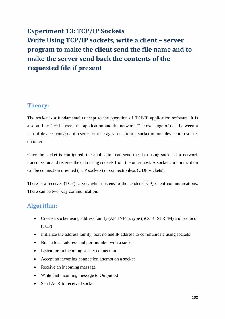
108
Experiment 13: TCP/IP Sockets
Write Using TCP/IP sockets, write a client – server
program to make the client send the file name and to
make the server send back the contents of the
requested file if present
Theory:
The socket is a fundamental concept to the operation of TCP/IP application software. It is
also an interface between the application and the network. The exchange of data between a
pair of devices consists of a series of messages sent from a socket on one device to a socket
on other.
Once the socket is configured, the application can send the data using sockets for network
transmission and receive the data using sockets from the other host. A socket communication
can be connection oriented (TCP sockets) or connectionless (UDP sockets).
There is a receiver (TCP) server, which listens to the sender (TCP) client communications.
There can be two-way communication.
Algorithm:
Create a socket using address family (AF_INET), type (SOCK_STREM) and protocol
(TCP)
Initialize the address family, port no and IP address to communicate using sockets
Bind a local address and port number with a socket
Listen for an incoming socket connection
Accept an incoming connection attempt on a socket
Receive an incoming message
Write that incoming message to Output.txt
Send ACK to received socket

109
Call step 5 to receive the message once again
Close file
Close socket
Procedure: To begin with the experiment, open NetSim
Click on Programming from the menu bar and select PC to PC Communication and then
select Socket Programming
When you select the User mode, you have to write your own program in C/C++, compile and
link to NetSim software for validation. Click on the F1 (Help) for details on how to proceed
with your own code.
The scenario will be obtained as shown below. Follow the steps
Under Input there are two things,
1. When Operation is Client, then the Server’s IP Address (Ex: 192.168.1.2) should
be given in the Server IP Address field.
Select Mode
Select Protocol
Select Operation
Click Run to
start
transmission Click here to
view Concept,
Algorithm, and
Pseudo Code &
Flowchart
Click here to
interface source
code

110
2. When Operation is Server, then the Server’s IP Address (Ex: 192.168.1.2) would
be automatically filled in the Local IP Address field.
If the Operation is Server, the scenario will be obtained as shown below,
If the Operation is Client, the scenario will be obtained as shown below,
Server
Side
Client
Side

111
TCP
First the Server should click on the Run button after which the Client should click on
the Run button to Create the socket
Client should click on the Connect button to establish the connection with server.
The Client should click on the Send button to transmit the data to the Server.
The Client should click on the Close button to terminate the Connection with Server.
If the Data is successfully transmitted then the Sent Data would be Received in the
Server System.
UDP
First the Server should click on the Run button after which the Client should click on
the Run button to Create the socket
The Client should click on the Send button to transmit the data to the Server.
The Client should click on the Close button to terminate the Connection with Server.
If the Data is successfully transmitted then the Sent Data would be Received in the
Server System.
Enter Destination
IP Address
Enter data to
be transmitted

112
Results:
Note- If using Dev C++ IDE, go to Tools->compiler options and add -lws2_32 as
follows before executing:
Received
data
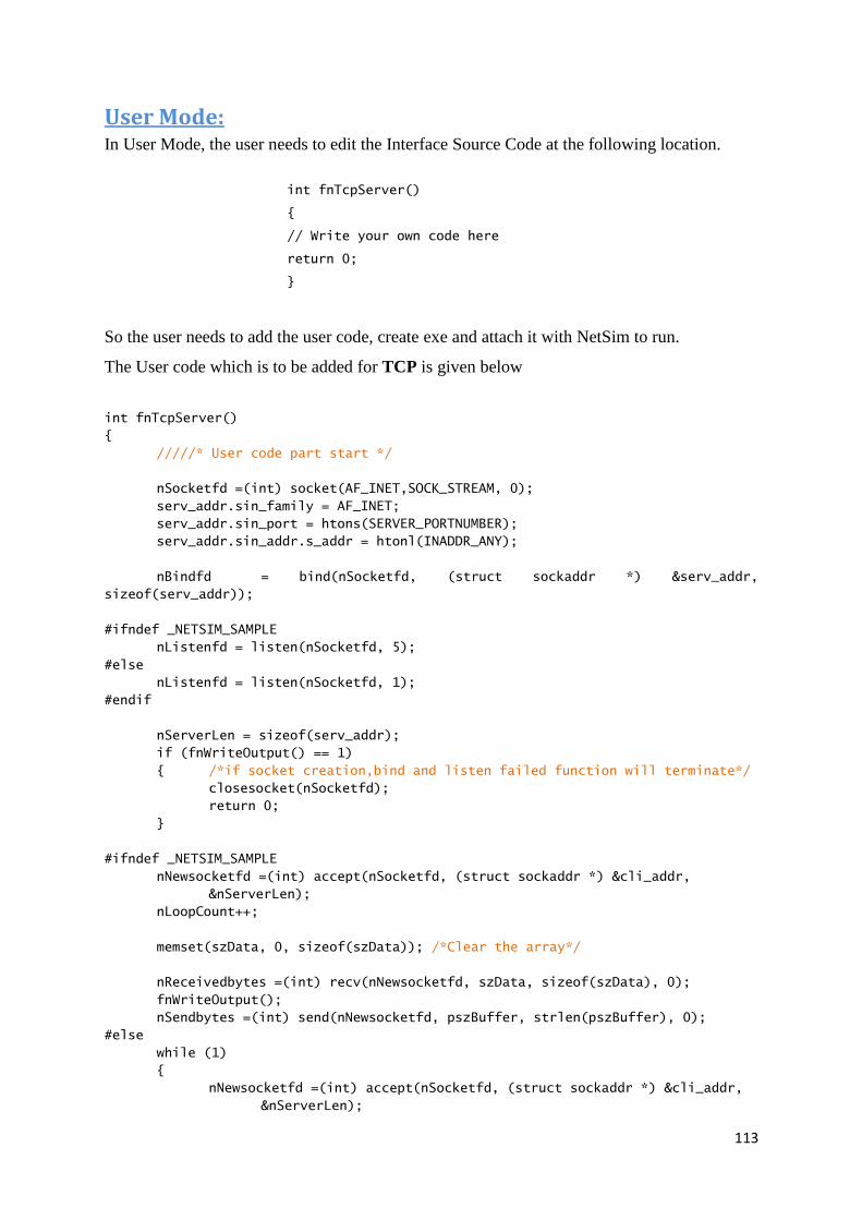
113
User Mode: In User Mode, the user needs to edit the Interface Source Code at the following location.
int fnTcpServer()
{
// Write your own code here
return 0;
}
So the user needs to add the user code, create exe and attach it with NetSim to run.
The User code which is to be added for TCP is given below
int fnTcpServer()
{
/////* User code part start */
nSocketfd =(int) socket(AF_INET,SOCK_STREAM, 0);
serv_addr.sin_family = AF_INET;
serv_addr.sin_port = htons(SERVER_PORTNUMBER);
serv_addr.sin_addr.s_addr = htonl(INADDR_ANY);
nBindfd = bind(nSocketfd, (struct sockaddr *) &serv_addr,
sizeof(serv_addr));
#ifndef _NETSIM_SAMPLE
nListenfd = listen(nSocketfd, 5);
#else
nListenfd = listen(nSocketfd, 1);
#endif
nServerLen = sizeof(serv_addr);
if (fnWriteOutput() == 1)
{ /*if socket creation,bind and listen failed function will terminate*/
closesocket(nSocketfd);
return 0;
}
#ifndef _NETSIM_SAMPLE
nNewsocketfd =(int) accept(nSocketfd, (struct sockaddr *) &cli_addr,
&nServerLen);
nLoopCount++;
memset(szData, 0, sizeof(szData)); /*Clear the array*/
nReceivedbytes =(int) recv(nNewsocketfd, szData, sizeof(szData), 0);
fnWriteOutput();
nSendbytes =(int) send(nNewsocketfd, pszBuffer, strlen(pszBuffer), 0);
#else
while (1)
{
nNewsocketfd =(int) accept(nSocketfd, (struct sockaddr *) &cli_addr,
&nServerLen);

114
nLoopCount++;
memset(szData, 0, sizeof(szData)); /*Clear the array*/
nReceivedbytes =(int) recv(nNewsocketfd, szData, sizeof(szData), 0);
fnWriteOutput();
nSendbytes =(int) send(nNewsocketfd, pszBuffer, strlen(pszBuffer),
0);
if( nTCPServerCloseFlag == 1) /*break the loop when user send
close the connection*/
break;
}
#endif
closesocket(nSocketfd);
/////* User code part end */
return 0;
}
The User code which is to be added for UDP is given below
int fnUdpServer()
{
/////* User code part start */
nSocketfd = (int)socket(AF_INET,SOCK_DGRAM, 0); /*Server side socket
creation*/
serv_addr.sin_family = AF_INET;
serv_addr.sin_addr.s_addr = htonl(INADDR_ANY);
serv_addr.sin_port = htons(SERVER_PORTNUMBER); /* Server port number 6000*/
nServerLen = sizeof(serv_addr);
nBindfd = bind(nSocketfd, (struct sockaddr *) &serv_addr,
sizeof(serv_addr));
fnWriteOutput();
#ifndef _NETSIM_SAMPLE
memset(szData, 0, sizeof(szData)); //Clear the array
nReceivedbytes = recvfrom(nSocketfd, szData, sizeof(szData), 0,(struct
sockaddr *) &serv_addr, &nServerLen);
fnWriteOutput();
#else
while(1)
{
memset(szData, 0, sizeof(szData)); //Clear the array
nReceivedbytes = recvfrom(nSocketfd, szData, sizeof(szData), 0,(struct
sockaddr *) &serv_addr, &nServerLen);
fnWriteOutput();
}
#endif
closesocket(nSocketfd);

115
/////* User code part end */
return 0;
}
Note- How to practice this experiment without using NetSim:
Users who do not have a licensed version of NetSim in their PC's, can practice as explained
below.
First, run the exercise in sample mode. The user would see that an Input.txt file is created in
Win OS temp folder (this can be reached by typing %temp%/NetSim in Windows run
window). This input file should be read by the user code and it should generate an Output.txt.
This Output.txt file is read by NetSim and shown graphically to the user.
User can follow the steps provided in Appendix 1: Programming exercise - How to practice
without NetSim.
Given below are sample Input.txt and Output.txt files for this experiment for users to verify
& validate their code. The Output.txt file will vary based on the Data_file. In this case, the
size of Data_File file is 11,264 bytes.
For TCP
Input.txt file contents at Server system
Protocol=TCP
Operation=Server
Input.txt file contents at Client system
Protocol=TCP
Operation=Client
Destination IP Address=192.168.0.130
192.168.0.147:-Hello World
Output.txt file contents at Server system
Socket Created
Bind Succeed
Listen Succeed
For UDP
Input.txt file contents at Server system
Protocol=UDP
Operation=Server
Input.txt file contents at Client system
Protocol=UDP
Operation=Client
Destination IP Address=192.168.0.130
192.168.0.147:-Hello World
Output.txt file contents at Server system
Socket Created
Bind Succeed

116
Experiment 14: RSA
Write a program for simple RSA algorithm to encrypt
and decrypt the data
Theory:
The Application Layer takes care of network security. Different encryption and decryption
techniques are used to provide security to the data that is to be transmitted.
Among these, is the public-key cryptography. Public-key cryptography requires each user to
have two keys: a public key, used by the entire world for encrypting messages to be sent to
the user; and a private key which the user needs for decrypting messages.
RSA algorithm was discovered at the Massachusetts Institute of Technology (MIT). RSA
stands for the initials of the three who discovered the algorithm: Rivest, Shamir and
Adleman.
Algorithm:
The technique followed is:
1. Choose two large primes, p and q, (typically greater than 10100
).
2. Compute n = p * q and z = ( p - 1 ) * ( q - 1 ).
3. Choose a number relatively prime to z and call it Kp.
4. Find Ks such that (Ks * Kp) mod z = 1.
To encrypt a message, P, compute C = PKs
(mod n). To decrypt C, compute P = CKp
(mod n).
It can be proven that for all P in the specified range, the encryption and decryption functions
are inversed. To perform the encryption, we need Ks and n. To perform the decryption, we
need Kp and n. Therefore, the public key consist of the pair (Ks,n) and the private key consist
of (Kp,n).

117
Procedure: To begin with the experiment, open NetSim
Click on Programming from the menu bar and select Cryptography and then select
AdvancedRSA
When you select the User mode, you have to write your own program in C/C++, compile and
link to NetSim software for validation. Click on the F1 (Help) for details on how to proceed
with your own code.
The scenario will be obtained as shown below. Follow the steps
Select Mode
Give Character
Click Run to execute
Click here to view
Concept, Algorithm, and
Pseudo Code & Flowchart
Click here to
Interface Source
Code
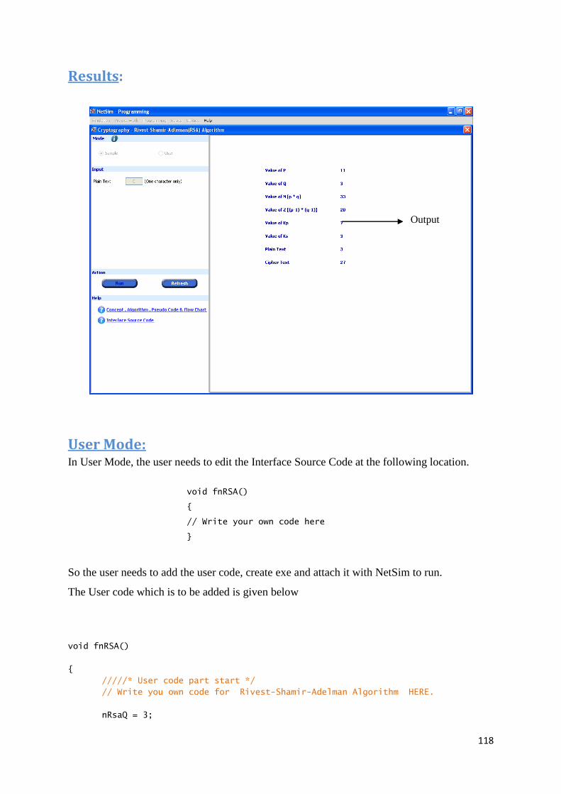
118
Results:
User Mode: In User Mode, the user needs to edit the Interface Source Code at the following location.
void fnRSA()
{
// Write your own code here
}
So the user needs to add the user code, create exe and attach it with NetSim to run.
The User code which is to be added is given below
void fnRSA()
{
/////* User code part start */
// Write you own code for Rivest-Shamir-Adelman Algorithm HERE.
nRsaQ = 3;
Output

119
nRsaP = 11;
nNVal = nRsaQ * nRsaP;
nZVal = (nRsaQ - 1) * (nRsaP - 1);
nKp = 7;
nKs = 3;
cChr = szStr[0];
//To get the Integer Equivalent Position of the Alphabets
// A=1, a=1, B=2, b=2, c=3, d=4 .......
nChr = cChr;
if ((nChr>=65) && (nChr<=90))
nChr = nChr - 64;
else if((nChr>=97) && (nChr<=122))
nChr= nChr - 96;
lCypTxt = fmod((long double) pow (nChr,nKs), (long double)nNVal);
lPlnTxt = fmod((long double) pow (lCypTxt,nKp), (long double)nNVal);
/////* User code part end */
}
Note- How to practice this experiment without using NetSim:
Users who do not have a licensed version of NetSim in their PC's, can practice as explained
below.
First, run the exercise in sample mode. The user would see that an Input.txt file is created in
Win OS temp folder (this can be reached by typing %temp%/NetSim in Windows run
window). This input file should be read by the user code and it should generate an Output.txt.
This Output.txt file is read by NetSim and shown graphically to the user.
User can follow the steps provided in Appendix 1: Programming exercise - How to practice
without NetSim.
Given below are sample Input.txt and Output.txt files for this experiment for users to verify
& validate their code. The Output.txt file will vary based on the Data_file. In this case, the
size of Data_File file is 11,264 bytes.
Input.txt file contents
Plain_Text=N
Output.txt file contents
11>3>33>20>7>3>5>14>

120
Experiment 15: Hamming Code
Write a program for Hamming code generation for
error detection and correction
Theory:
Hamming code is for Single Bit Error Detection and Correction. It is based on Parity (Even /
Odd Parity).
It allows any single bit error to be detected and corrected. It involves adding one or four
check bits (depending on the formula) to the data for error detection as well as error
correction. These bits are called Check Bits. In order to find the number of check bits
introduced in the message bits, there is a general formula.
For a message of size m bits and r check bits, then the condition (m + r + 1) < = 2 r should be
valid.
Example:
Consider the message size (m) of 4 bits and we will find out the number of check bits
according to the formula,
When r = 3 we have, 4 + 3 + 1 = 8 and 2 3 is 8 and so the number of Check Bits to be
introduced is 3.
Algorithm:
Read the contents of the input file i.e. the input data, type of parity and the error data from the
„Input.txt‟ and store it in variables like the above method.
1. Get the length of the input data and calculate the number of Check Bits to be
introduced according to the condition (m + r + 1) <= 2r. Where m is length of the
original data and r is the number of check bits to be introduced in the string.
2. If the passed flag (type of parity) is 2, then it is Even parity, else it is Odd parity.

121
3. Place the Check Bits at the appropriate position according to the principle explained
above (Calculation and Placement of Check Bits in Hamming Code) for the Input data
and for the Error data.
4. Compare the Check Bits values of the Original Input Data and the Error Data values.
Keep a note of the Check Bit Position where the value differs.
5. Add all the position of the Check Bits where the values differ. The resultant value
gives the position of the error bit in the Error Data of length ( m + r ) i.e. the total
length which includes the length of the Input Data Bits and the Check Bits.
Procedure: To begin with the experiment, open NetSim
Click on Programming from the menu bar and select Error Correcting Code and then select
Hamming Code
When you select the User mode, you have to write your own program in C/C++, compile and
link to NetSim software for validation. Click on the F1 (Help) for details on how to proceed
with your own code. The scenario will be obtained as shown below. Follow the steps
Step 1:
Select the
Mode
Select
the Parity

122
Step 2:
After that you can type the input in the Textbox and Select the error position which is shown
below
Enter the Data
Select the Error
Position
Click run to execute
Click here to view the Concept,
Algorithm, Pseudo code and Flow
chart
Click here to Interface
Source Code
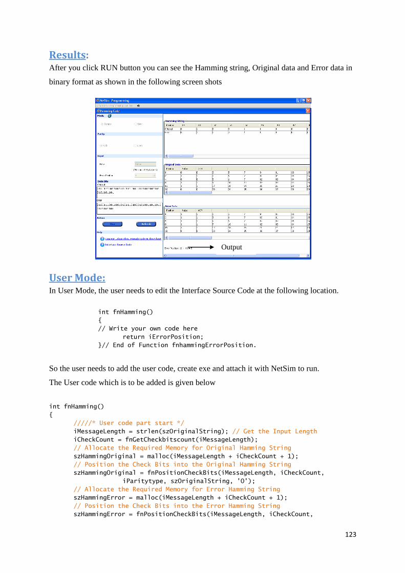
123
Results: After you click RUN button you can see the Hamming string, Original data and Error data in
binary format as shown in the following screen shots
User Mode: In User Mode, the user needs to edit the Interface Source Code at the following location.
int fnHamming()
{
// Write your own code here
return iErrorPosition;
}// End of Function fnhammingErrorPosition.
So the user needs to add the user code, create exe and attach it with NetSim to run.
The User code which is to be added is given below
int fnHamming()
{
/////* User code part start */
iMessageLength = strlen(szOriginalString); // Get the Input Length
iCheckCount = fnGetCheckbitscount(iMessageLength);
// Allocate the Required Memory for Original Hamming String
szHammingOriginal = malloc(iMessageLength + iCheckCount + 1);
// Position the Check Bits into the Original Hamming String
szHammingOriginal = fnPositionCheckBits(iMessageLength, iCheckCount,
iParitytype, szOriginalString, 'O');
// Allocate the Required Memory for Error Hamming String
szHammingError = malloc(iMessageLength + iCheckCount + 1);
// Position the Check Bits into the Error Hamming String
szHammingError = fnPositionCheckBits(iMessageLength, iCheckCount,
Output

124
iParitytype, szErrorString, 'E');
// Get the error position
iErrorPosition = fnErrorPosition(szHammingOriginal, szHammingError, strlen(
szHammingOriginal), iCheckCount);
/////* User code part end */
return iErrorPosition;
}// End of Function fnhammingErrorPosition.
Note- How to practice this experiment without using NetSim
Users who do not have a licensed version of NetSim in their PC's, can practice as explained
below. First, run the exercise in sample mode. The user would see that an Input.txt file is
created in Win OS temp folder (this can be reached by typing %temp%/NetSim in Windows
run window). This input file should be read by the user code and it should generate an
Output.txt. This Output.txt file is read by NetSim and shown graphically to the user.
User can follow the steps provided in Appendix 1: Programming exercise - How to practice
without NetSim.
Given below are sample Input.txt and Output.txt files for this experiment for users to verify
& validate their code
Input.txt file contents
Parity=Odd
Data=ABC
Error_Position=1
Data_Bits_Original=010000010100001001000011
Data_Bits_Error=010000010100001001000010
Output.txt file contents
5
3>5>7>9>11>13>15>17>19>21>23>25>27>29>1>1>
3>6>7>10>11>14>15>18>19>22>23>26>27>30>1>1>
5>6>7>12>13>14>15>20>21>22>23>28>29>30>1>1>
9>10>11>12>13>14>15>24>25>26>27>28>29>30>1>1>
17>18>19>20>21>22>23>24>25>26>27>28>29>30>1>1>
3>5>7>9>11>13>15>17>19>21>23>25>27>29>0>0>
3>6>7>10>11>14>15>18>19>22>23>26>27>30>1>1>
5>6>7>12>13>14>15>20>21>22>23>28>29>30>0>0>
9>10>11>12>13>14>15>24>25>26>27>28>29>30>1>1>
17>18>19>20>21>22>23>24>25>26>27>28>29>30>1>1>
1>4>5>

125
Experiment 16: Leaky Bucket Algorithm
Write a program for congestion control using leaky
bucket algorithm.
Theory:
1. This is a type of traffic shaping algorithm. Traffic shaping allows control of the traffic
in the network to improve performance of the network.
2. An application before transmitting, agrees upon a peak cell rate. This algorithm will
not allow packets more than the agreed peak cell rate.
3. This algorithm will also avoid burst of data arrival which could lead to congestion.
4. One of the major reasons for congestion is the burst kind of data arrival in the
network. This algorithm is used to avoid the burst traffic.
5. Burst input data is stored in a buffer and output at a constant rate. If the input rate is
larger than the output rate and the buffer is full, the extra data is discarded and not
transmitted.
Algorithm:
1. Read data „Input.txt‟ file, which has the required data.
2. Parse the content of the file from which you get the input rate for each second, buffer
size, output rate per second and store in separate variables.
3. Follow the steps outlined below for time starting from 0 to 10.
4. If input rate is larger than the output rate, less the output rate (store the rate of packet
output for the corresponding second) and for the remaining input packets, check for
buffer availability.
5. If the buffer value is larger than or equal to the remaining input packets, store the
remaining packets in the buffer. Else, if the buffer capacity is lesser, then store up to
the capacity of the buffer and discard the rest of the packets. Increment timer.

126
6. If the input rate is equal to the output rate, no packet is stored in the buffer. (Store the
output rate, discard packet as zero, for the corresponding second). Increment timer.
7. If the input rate is less than the output rate, no packet is stored in the buffer. (Store the
input rate as output rate, discard packet as zero, for the corresponding second).
Increment timer.
8. Follow the steps outlined below until buffer capacity is zero.
9. If the buffer value is non-zero, reduce the buffer capacity by the output rate – if the
buffer value is more than the output rate. (Store the output rate, discard packet as zero,
for the corresponding second). Increment timer.
10. If the buffer value is non-zero, reduce the buffer capacity to 0 if the buffer value is
less than or equal to the output rate. (Store the buffer capacity; discard the packet as
zero for the corresponding second). Increment timer.
11. Store the total time value.
12. Write the required values to the output file „Output.txt‟.
Procedure: To begin with the experiment, open NetSim
Click on Programming from the menu bar and select Leaky Bucket Algorithm.
When you select the User mode, you have to write your own program in C/C++, compile and
link to NetSim software for validation. Click on the F1 (Help) for details on how to proceed
with your own code.
The scenario will be obtained as shown below. Follow the steps

127
Results:
Select Mode
Give Input capacity
Give Output capacity
Give Buffer capacity
Click run to execute
Click here to Concept, Algorithm,
and Pseudo Code & Flow Chart
Click here to Interface
Source Code
Output

128
User Mode: In User Mode, the user needs to edit the Interface Source Code at the following location.
void fnLBA()
{
// Write your own code here
}
So the user needs to add the user code, create exe and attach it with NetSim to run.
The User code which is to be added is given below
void fnLBA()
{
/////* User code part start */
// Write you own code for Leaky Bucket algorithm HERE.
int nBufferValue = 0;
int nInterval = 0;
nSeconds = 0;
for (nInterval = 0; nInterval < 10; nInterval++) {
if ((nInputRate[nInterval] - nOutputRate) > 0) // the input is more
than the output rate
{
if ((nBufferValue + (nInputRate[nInterval] - nOutputRate))
>= nBufferSize) // All put together the value is
more or equal than the buffer size
{
if ((nBufferValue + (nInputRate[nInterval] -
nOutputRate))
> nBufferSize) // more than case where we
have discard
nDiscardRate[nSeconds] = (((nInputRate[nInterval]
- nOutputRate) + nBufferValue) -
nBufferSize);// the discard rate is recorded
nBufferValue = nBufferSize;
} else
// this equal case is where we have no discard
nBufferValue = nBufferValue + (nInputRate[nInterval]
- nOutputRate); // the exces is stored in
the buffer
// for both case the output and buffer level is recorded
nOutputRates[nSeconds] = nOutputRate;
} else if ((nInputRate[nInterval] - nOutputRate) == 0) // the output
is equal to input rate
{
nBufferValue = nBufferValue;
nOutputRates[nSeconds] = nOutputRate;

129
} else if ((nInputRate[nInterval] - nOutputRate) < 0) // input is
less than output rate
{
if (nInputRate[nInterval] > 0) {
if ((nBufferValue + (nInputRate[nInterval] -
nOutputRate))
>= nBufferSize)// All put together the
value is more or equal than the buffer size
{
if ((nBufferValue + (nInputRate[nInterval] -
nOutputRate))
> nBufferSize)// more than case
where we have discard
nDiscardRate[nSeconds] =
(((nInputRate[nInterval]
- nOutputRate) + nBufferValue)
- nBufferSize);// the discard rate is recorded
nBufferValue = nBufferSize;
nOutputRates[nSeconds] = nOutputRate;
} else {
if ((nBufferValue + (nInputRate[nInterval] -
nOutputRate))
<= 0) {
nOutputRates[nSeconds] = nBufferValue
+ nInputRate[nInterval];
nBufferValue = 0;
} else {
nOutputRates[nSeconds] = nOutputRate;
nBufferValue = nBufferValue +
(nInputRate[nInterval]
- nOutputRate);
}
}
} else {
if ((nBufferValue - nOutputRate) > 0) {
nBufferValue = nBufferValue - nOutputRate;
nOutputRates[nSeconds] = nOutputRate;
} else {
nOutputRates[nSeconds] = nBufferValue;
nBufferValue = 0;
}
}
}
nBufferLevel[nSeconds] = nBufferValue;
nSeconds++;
}
while (nBufferValue != 0)// this sends the remaining data in the buffer

130
{
if (nBufferValue > nOutputRate) // buffer is more than the output
{
nBufferValue = nBufferValue - nOutputRate;
nOutputRates[nSeconds] = nOutputRate;
} else
{
nOutputRates[nSeconds] = nBufferValue;
nBufferValue = 0;
}
nBufferLevel[nSeconds] = nBufferValue;
nSeconds++;
}
// Write you own code for Leaky Bucket algorithm HERE.
/////* User code part end */
}
Note- How to practice this experiment without using NetSim:
Users who do not have a licensed version of NetSim in their PC's, can practice as explained
below. First, run the exercise in sample mode. The user would see that an Input.txt file is
created in Win OS temp folder (this can be reached by typing %temp%/NetSim in Windows
run window). This input file should be read by the user code and it should generate an
Output.txt. This Output.txt file is read by NetSim and shown graphically to the user.
User can follow the steps provided in Appendix 1: Programming exercise - How to practice
without NetSim.
Given below are sample Input.txt and Output.txt files for this experiment for users to verify
& validate their code. The Output.txt file will vary based on the Data_file. In this case, the
size of Data_File file is 11,264 bytes.
Input.txt file contents
Output_Capacity=100
Buffer_Size=100
Input_Capacity=100,200,120,400,100,600,100,100,100,100,
Output.txt file contents
100>100>100>100>100>100>100>100>100>100>100>
0>0>20>300>0>500>0>0>0>0>0>
11>
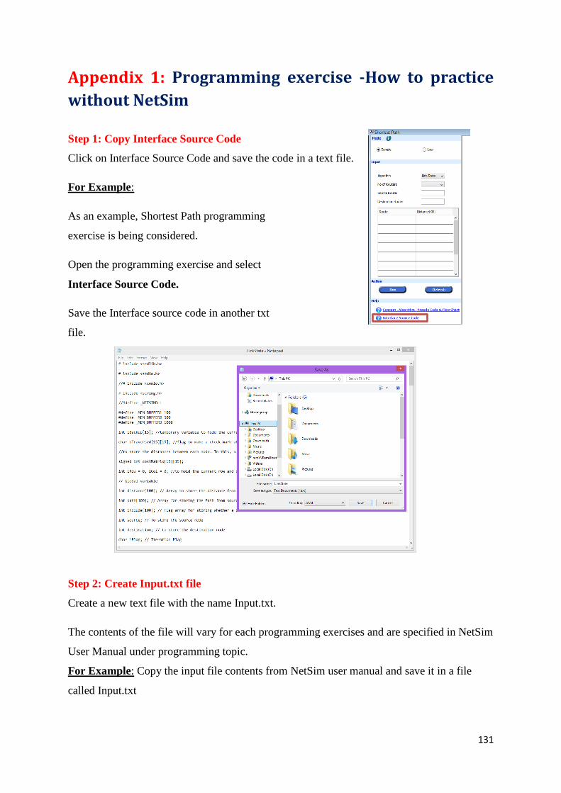
131
Appendix 1: Programming exercise -How to practice
without NetSim
Step 1: Copy Interface Source Code
Click on Interface Source Code and save the code in a text file.
For Example:
As an example, Shortest Path programming
exercise is being considered.
Open the programming exercise and select
Interface Source Code.
Save the Interface source code in another txt
file.
Step 2: Create Input.txt file
Create a new text file with the name Input.txt.
The contents of the file will vary for each programming exercises and are specified in NetSim
User Manual under programming topic.
For Example: Copy the input file contents from NetSim user manual and save it in a file
called Input.txt

132
Sample:
Algorithm=Link_State
No_of_Router=3
Distance:
999>6>5>
6>999>7>
5>7>999>
Source_Router=1
Destination_Router=2
Save it in some other location. In this example, it is saved at D:\New.
Step 3: Create .exe file
Open C editor (Turbo C, Dev C++, etc) and write the Interface source code which was saved
in the first text file. Also add the code to be written by the user in the specific sections and
compile it. Keep the .exe file.
For Example:
Now in C editor (Dev C++ IDE is used here), copy the interface source code. In the interface
source code, void fnDijkstra() is not implemented.

133
After writing the code for the function void fnDijkstra(), create .exe file. The procedure to
create .exe file is explained in Section 9.2 of NetSim User Manual.
In this example, the exe file created is LinkState.exe
Step 4: Run in command prompt
Open command prompt, and go to the folder where the .exe file is saved.
There type
<EXE Name> “<blank>“ “<Path where Input.txt is saved>”;
For Example:
In this example, the exe file LinkState.exe and Input.txt is present at “D:\New”. So in
command prompt go to the folder where exe file is saved.
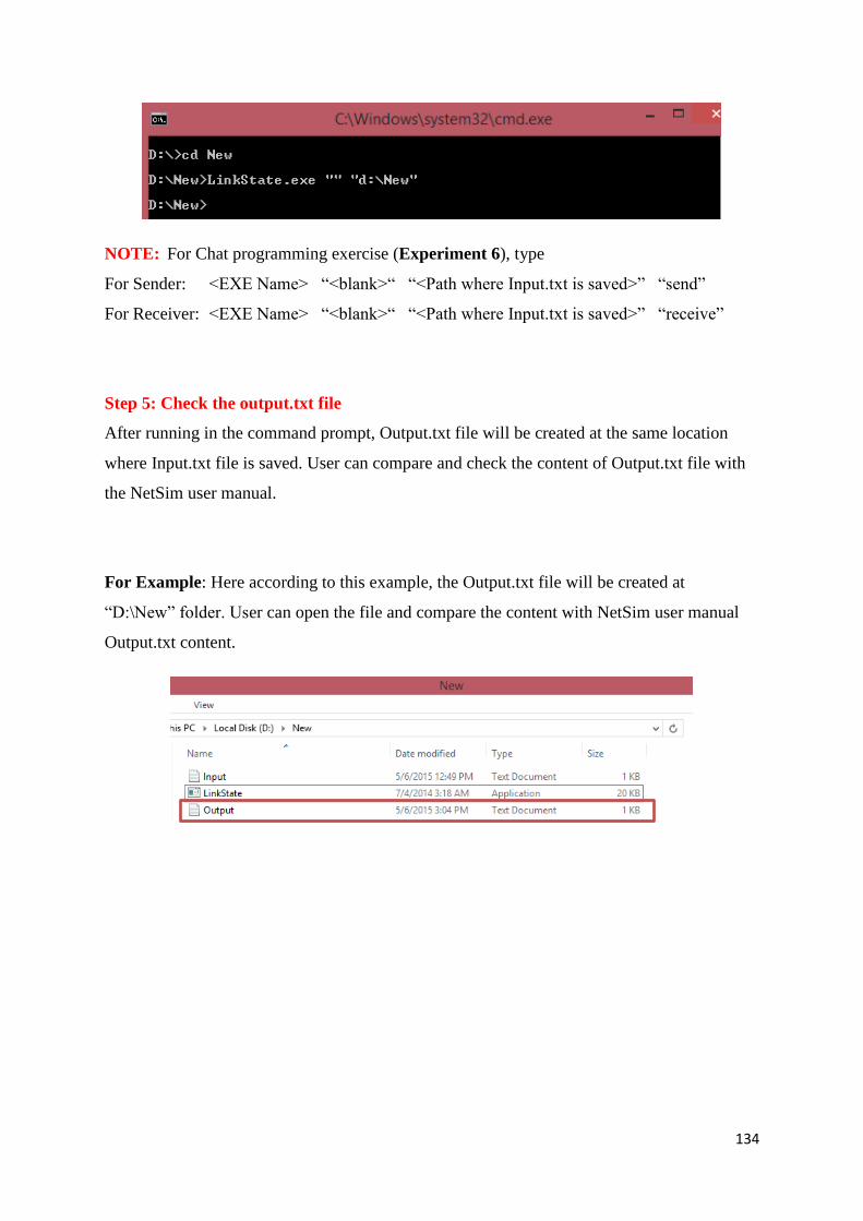
134
NOTE: For Chat programming exercise (Experiment 6), type
For Sender: <EXE Name> “<blank>“ “<Path where Input.txt is saved>” “send”
For Receiver: <EXE Name> “<blank>“ “<Path where Input.txt is saved>” “receive”
Step 5: Check the output.txt file
After running in the command prompt, Output.txt file will be created at the same location
where Input.txt file is saved. User can compare and check the content of Output.txt file with
the NetSim user manual.
For Example: Here according to this example, the Output.txt file will be created at
“D:\New” folder. User can open the file and compare the content with NetSim user manual
Output.txt content.

135
Appendix 2: Creating .exe file using Dev C++
1. Open the C source code file in Dev C++. Then go to Execute Compile.
Dev C++ will create the exe file in the same location where the C source code file is
located
2. Once exe file is created , link that exe file with NetSim Programming User mode
Note: For Windows 8 and above, use Dev C++ v 5.11
Note: For Windows Vista, set up Dev C++ as shown below
In Dev C++ 4.9.9.2.exe, go to Tools->Compiler Options->Directories tab->Binaries tab
Add the following path as per your installation directory in the text box provided and click on
add button.
C:\Dev-Cpp\libexec\gcc\mingw32\3.4.2

136
In the C Includes tab add the follwing path in the text box provided and click on add button.
C:\Dev-Cpp\lib\gcc\mingw32\3.4.2\include
In the programs tab edit the following paths as shown in screenshot.

137