Experiment 3 Getting Start with...

13A.ALASHQAR & A.KHALIFEH

CME312- LAB Manual Getting Start with Simulink Experiment 3

Objectives :

By the end of this experiment, the student should be able to:

1. Build and simulate simple system model using Simulink

2. Use Simulink test and measurement tools.

1. Introduction

Simulink is a program for simulating signals and dynamic systems. Simulink has two

phases of use: model definition and model analysis. It provides an interactive

graphical environment and a customizable set of block libraries that let you design,

simulate, implement, and test a variety of time-varying systems, including

communications, controls, signal processing, video processing, and image processing.

Simulink provides toolboxes for designing, simulating, and analyzing communications

systems. The Simulink enables source coding, channel coding, interleaving, analog and

digital modulation, equalization, synchronization, and channel modeling.

A typical session starts by either defining a new model or by recalling a previously

defined model, and then proceeds to analyze that model. In order to facilitate the

model definition, Simulink has a large library of blocks. Models are created by

combining proper blocks from the library and edited in the model window principally

using mouse-driven operation ( Drag and Drop ) . An important part of mastering

Simulink is to become familiar with manipulations of various model components in

these windows.

After you create (or define) a model, you can analyze it either by choosing options

from the Simulink menus in the model window or by entering commands in the Matlab

command window. The progress of an ongoing simulation can be viewed while it is

running, and the final results can be made available in the Matlab workspace when the

simulation is complete.

Experiment 3

Experiment 2

Getting Start with Simulink



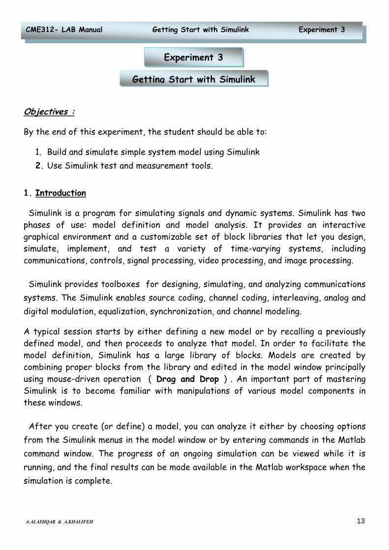
1.1 Starting Simulink:

1. Start up Matlab.

2. Start up Simulink by clicking the Simulink icon or by typing >>Simulink at

the Matlab command window.

3. You should see the Simulink Block Library window as shown in figure 1.



1.3 The Simulink Library

The Simulink Library Browser is the library where you find all the blocks you may use

in Simulink. Simulink software includes an extensive library of functions commonly

used in modeling a system. These include:



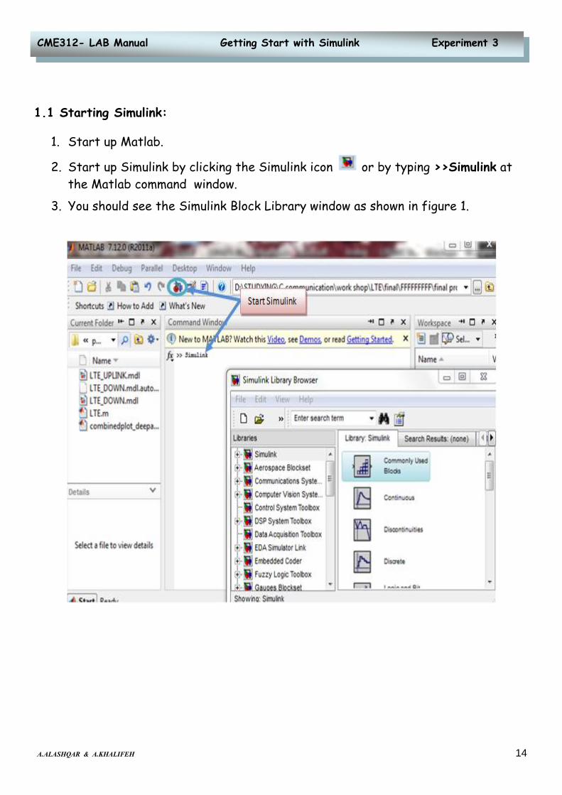
1.3.1 Common Block Libraries:

In this section we will see the most common used block libraries in communication

system models.

1. Commonly Used Block

2. Continuous :



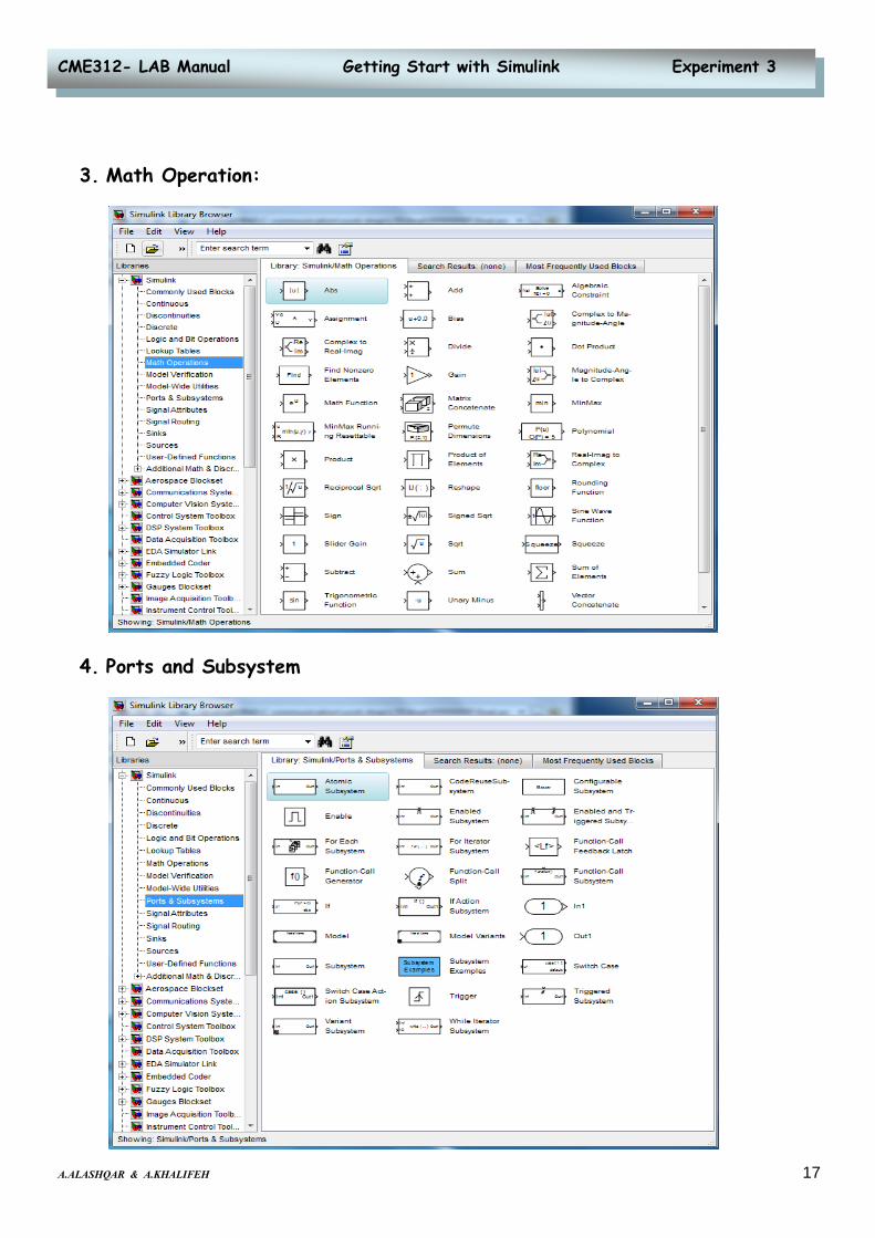
3. Math Operation:

4. Ports and Subsystem



5. Signal Routing

6. Sinks



7. Sources



1.4 Communications System Toolbox

Communications System Toolbox provides algorithms for designing, simulating, and

analyzing communications systems. The system toolbox enables source coding, channel

coding, interleaving, modulation, equalization, synchronization, and channel modeling.

You can also analyze bit error rates, generate eye and constellation diagrams, and

visualize channel characteristics. Using adaptive algorithms, you can model dynamic

communications systems that use OFDM, OFDMA, and MIMO techniques. Algorithms

support fixed-point data arithmetic and C or HDL code generation.



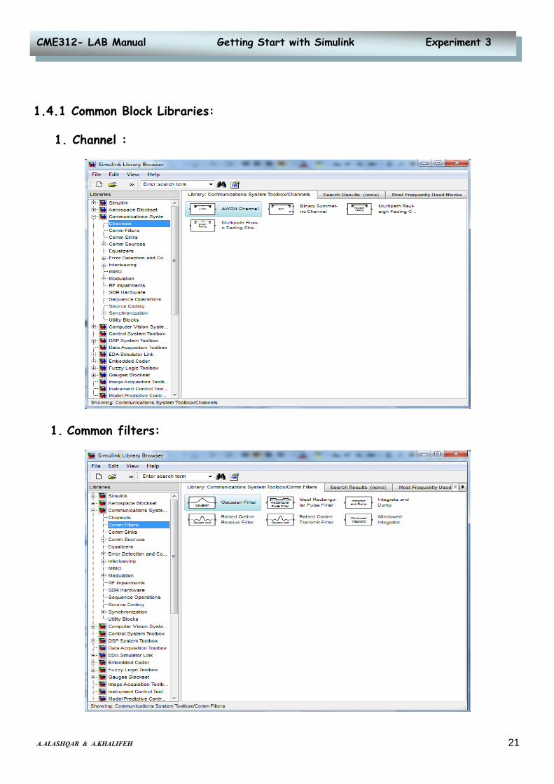
1.4.1 Common Block Libraries:

1. Channel :

1. Common filters:



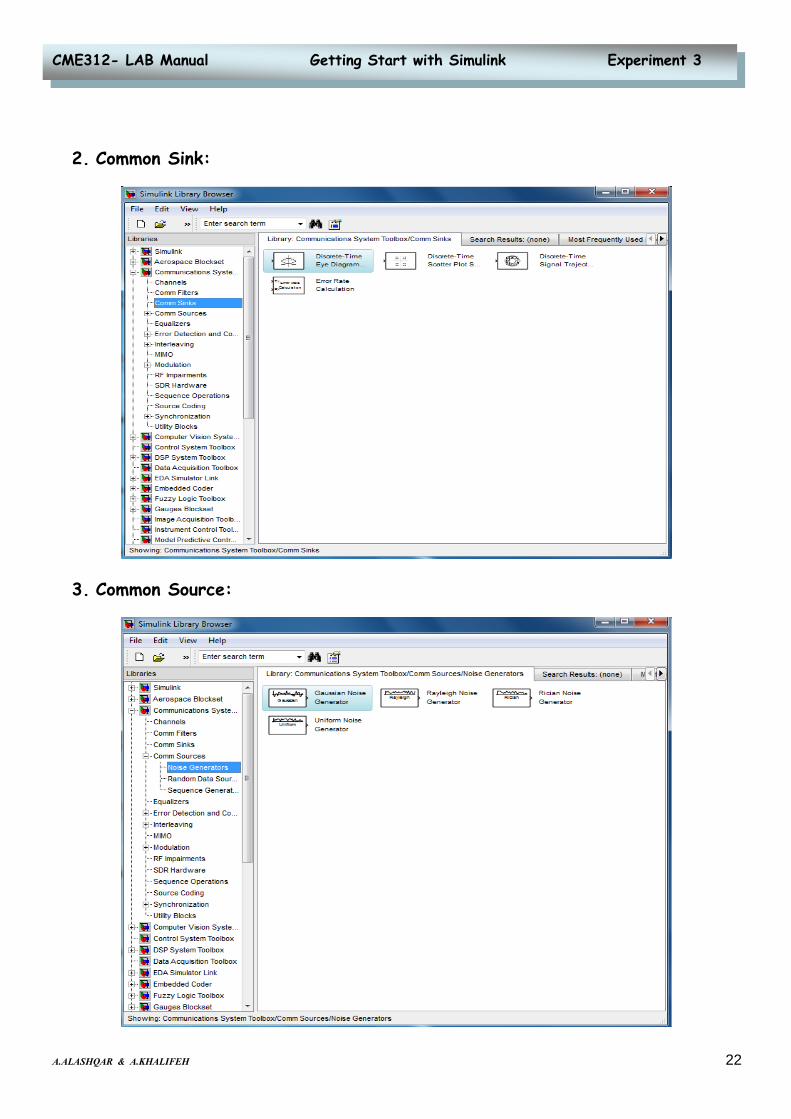
2. Common Sink:

3. Common Source:



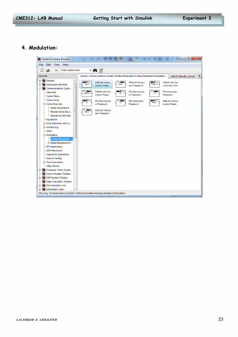
4. Modulation:



1.5 DSP System Toolbox

DSP System Toolbox provides algorithms for designing and simulating signal

processing systems. he system toolbox includes design methods for filters, FFTs,

multirate processing, and DSP techniques for processing streaming data and creating

real-time prototypes. You can design adaptive and multirate filters, implement filters

using computationally efficient architectures, and simulate floating-point digital

filters. Tools for signal I/O from files and devices, signal generation, spectral

analysis, and interactive visualization enable you to analyze system behavior and

performance. For rapid prototyping and embedded system design, the system toolbox

supports fixed-point arithmetic and C or HDL code generation.



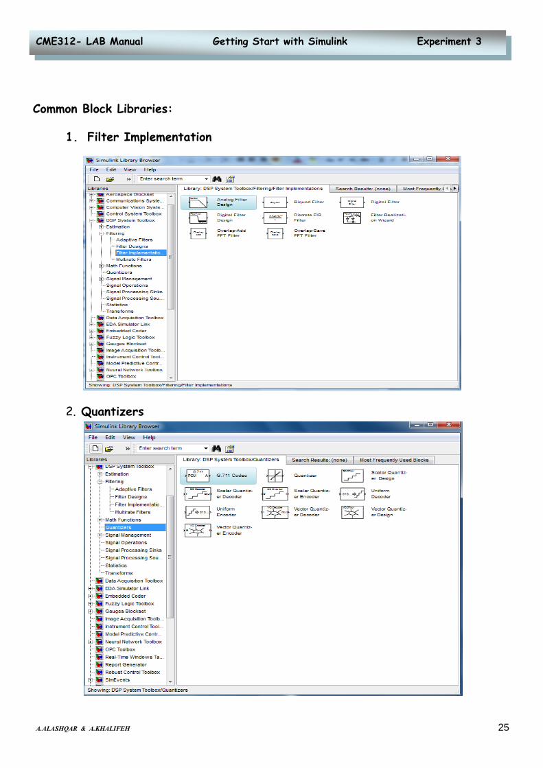
Common Block Libraries:

1. Filter Implementation

2. Quantizers



3. Signal Processing Sinks



1.6 Building a Simple Model

The Basic Steps

This section describes the basic steps in building a model. It explains how to:

Open a new model window

Open block libraries

Move blocks into a model window

Connect the blocks

Set block parameters

Set simulation parameters

Run the model

1. Opening a New Model Window

The first step in building a model is to open a new model window. To do so, by clicking

the new form icon or select New from the File menu, and then select Model. This

opens an empty model window, as shown in the following figure.



2. Opening Block Libraries

The next step is to select the blocks for the model. These blocks are contained in

libraries. To view the libraries for the products you have installed, type Simulink at

the MATLAB prompt (or, on Microsoft Windows, click the Simulink button on the

MATLAB toolbar).

3. Simulink Library Browser

The left pane displays the installed products, each of which has its own library of

blocks. To open a library, click the plus sign (+) next to the name of the blockset in

the left pane. This displays the contents of the library in the right-hand pane. You

can find the blocks you need to build models of communication systems in the

libraries of the Communications System Toolbox, the DSP Toolbox Blockset, and

Simulink.



4. Moving Blocks into the Model Window

The next step in building the model is to move blocks from the Simulink Library

Browser into the model window. To do so,

1. Click the + sign next to Simulink in the left pane of the Library Browser. This

displays a list of the Signal Processing Blockset libraries.

2. Click Sources in the left pane. This displays a list of the Sources library

blocks in the right pane.

3. Click the Sine Wave block and Drag and Drop it into the model window.

4. Click Sinks in the left pane of the Library Browser. This displays a list of the

Sinks library blocks in the right pane.

5. Click the Scope Block and drag and Drop it into the model window.



5. Connecting Blocks

The small arrowhead pointing outward from the right side of the Sine Wave block is

an output port for the data the block generates. The arrowhead pointing inward on

the Scope block is an input port.

To connect the two blocks, click the output port of the SineWave block and drag the

mouse toward the input port of the Vector Scope block, as shown in the following

figure.

When the pointer is on the input port of the Vector Scope block, release the mouse

button. You should see a solid arrow appear, as in the following figure.

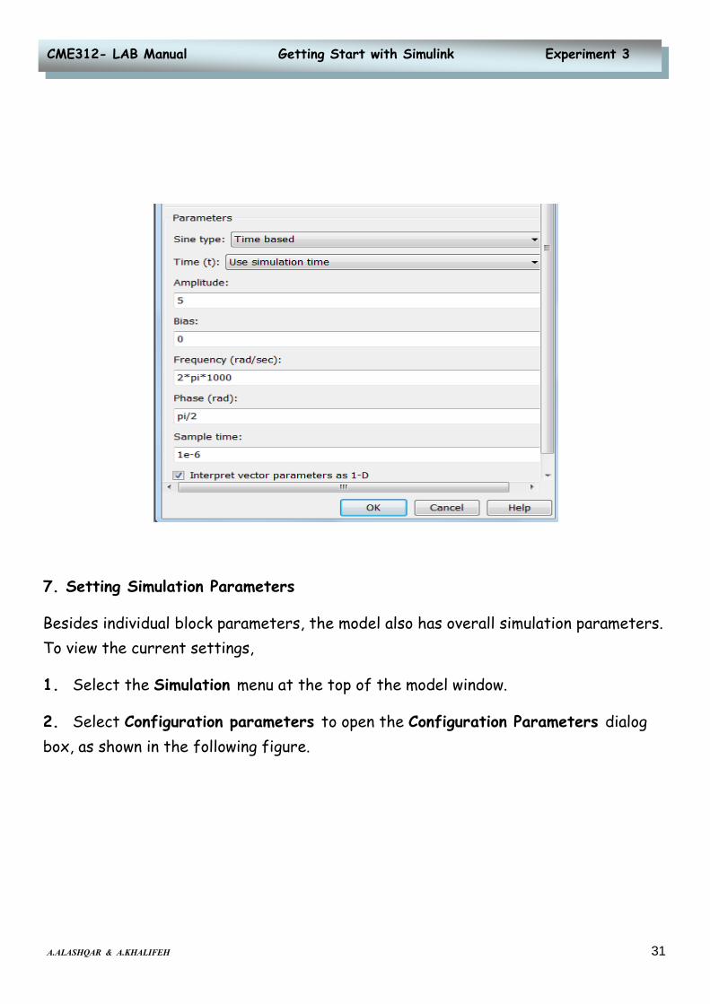
6. Setting Block Parameters

To set parameters for the Sine Wave block, double-click the block to open its dialog,

as shown in the following figure. Change the following parameters by clicking in the

field next to the parameter, deleting the default setting, and entering the new

setting in its place:



7. Setting Simulation Parameters

Besides individual block parameters, the model also has overall simulation parameters.

To view the current settings,

1. Select the Simulation menu at the top of the model window.

2. Select Configuration parameters to open the Configuration Parameters dialog

box, as shown in the following figure.



The Stop time determines the time at which the simulation ends. Setting Stop time

to inf causes the simulation to run indefinitely, until you stop it by selecting Stop

from the Simulation menu.

The Stop time is not the actual time it takes to run a simulation. The actual run-time

for a simulation depends on factors such as the model’s complexity and your

computer’s clock speed. The settings in the Configuration Parameters dialog box

affect only the parameters of the current model.

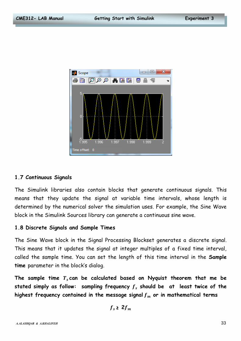
8. Running the Model

Run the model by clicking start simulation icon or selecting Start from the

Simulation menu. When you do so, a scope window appears, displaying a sine wave as

shown in the following figure.



1.7 Continuous Signals

The Simulink libraries also contain blocks that generate continuous signals. This

means that they update the signal at variable time intervals, whose length is

determined by the numerical solver the simulation uses. For example, the Sine Wave

block in the Simulink Sources library can generate a continuous sine wave.

1.8 Discrete Signals and Sample Times

The Sine Wave block in the Signal Processing Blockset generates a discrete signal.

This means that it updates the signal at integer multiples of a fixed time interval,

called the sample time. You can set the length of this time interval in the Sample

time parameter in the block’s dialog.

The sample time 𝑻𝒔 can be calculated based on Nyquist theorem that me be

stated simply as follow: sampling frequency 𝒇𝒔 should be at least twice of the

highest frequency contained in the message signal 𝒇𝒎 or in mathematical terms

𝒇𝒔 ≥ 2𝒇𝒎



𝑻𝒔 =𝟏

𝒇𝒔

Note

Many blocks in the Communications Blockset accept only discrete signals. To find out

whether a block accepts continuous signals, consult the reference page for the block.

1.9 Frames and Frame-Based Processing

A frame is a sequence of samples combined into a single vector. By setting Samples

per frame to 100 in the Sine Wave block, you set the frame size to 100, so that each

frame contains 100 samples. This enables the Vector Scope block to display enough

data for a good picture of the sine wave.

Another important reason to set the frame size is that many Communications

Blockset blocks require their inputs to be vectors of specific sizes. If you connect a

source block, such as the Sine Wave block, to one of these blocks, you can set the

input size correctly by setting Samples per frame to the required value. The model

described in “Reducing the Error Rate Using a Hamming Code” shows how to do this.

In frame-based processing all the samples in a frame are processed simultaneously. In

sample-based processing, on the other hand, samples are processed one at a time. The

advantage of frame-based processing is that it can greatly increase the speed of a

simulation. If you see double lines between blocks, the model uses frame-based

processing.

Time and Spectral Analysis

This section deals with looking at the waveforms of simple sine wave and pulse wave.

Figure 2.1 shows the design for viewing the waveforms of toe signals.



The blocks parameters:



The results:



Spectrum Scope

This section deals with looking at the spectrum of simple waves. We first look at the

spectrum of a simple sine wave.

Spectrum of a simple sine wave: - Figure 1.2 shows the design for viewing the

spectrum of a simple sine wave.

Parameters:

The sine wave block parameters as shown in



The frequency domain spectrum is obtained through a buffered-FFT scope, which

comprises of a Fast Fourier Transform of 128 samples which also has a buffering of

128 of them in one frame. The property block of the B-FFT is also displayed in figure

1.5.



Result:

The below figure shows the frequency domain corresponding of the sine wave

Notes:

From the property box of the B-FFT scope the axis properties can be changed

and the Line properties can be changed. The line properties are not shown in

the above. The Frequency range can be changed by using the frequency range

pop down menu and so can be the y-axis the amplitude scaling be changed to

either real magnitude or the dB (log of magnitude) scale. The upper limit can be

specified as shown by the Min and Max Y-limits edit box. The sampling time in

this case has been set to 1/3000.

The sampling frequency of the B-FFT scope should match with the sampling

time of the input time signal.

Also as indicated above the FFT is taken for 128 points and buffered with half

of them for an overlap.

Calculating the Power: The power can be calculated by squaring the value of the

voltage of the spectrum analyzer.

Note: The signal analyzer if chosen with half the scale, the spectrum is the

single-sided analyzer, so the power in the spectrum is the total power.

Similar operations can be done for other waveforms – like the square wave,

triangular. These signals can be generated from the signal generator block.



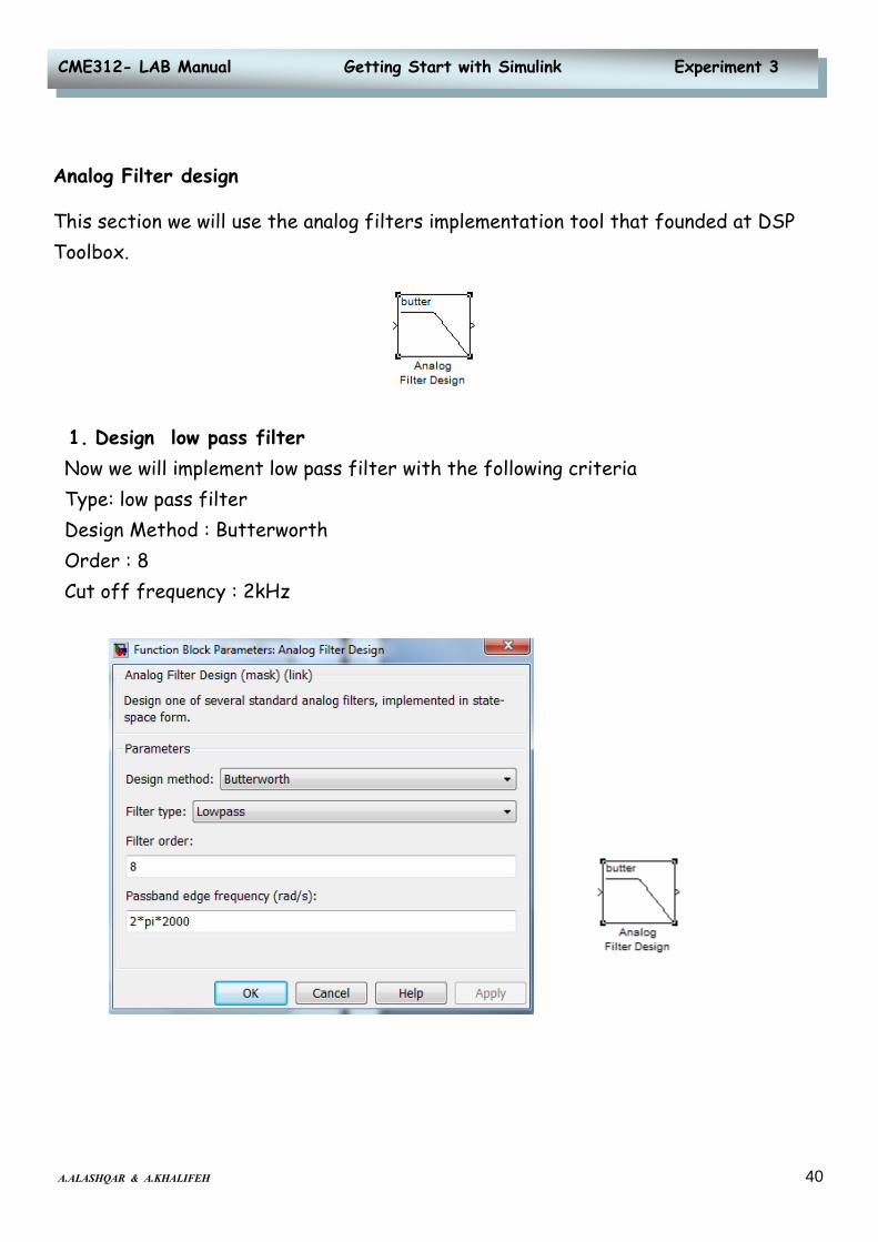
Analog Filter design

This section we will use the analog filters implementation tool that founded at DSP

Toolbox.

1. Design low pass filter

Now we will implement low pass filter with the following criteria

Type: low pass filter

Design Method : Butterworth

Order : 8

Cut off frequency : 2kHz



2. Design High Pass Filter

In the same manner we will implement high pass filter with the following criteria :

Type: high pass filter


Order : 8

Cut off frequency : 10kHz



3. Design Band Pass Filter

Finally we will implement band pass filter with the following criteria :

Type: band pass filter


Order : 8

lower Cut off frequency : 2KHz

upper cut off frequency :10kHz

Experiment 3 Getting Start with...

Documents

Transcript of Experiment 3 Getting Start with...