Document de treball 2005/3:

Expenditure spillovers and fiscal interactions: Empirical evidence from local governments in Spain

Albert Solé Ollé

Institut d'Economia de Barcelona Espai de Recerca en Economia

Facultat de Ciències Econòmiques i Empresarials Universitat de Barcelona

Av. Diagonal, 690 08034 Barcelona

Tel.: 93 403 46 46 Fax: 93 402 18 13

E-mail: ieb@pcb.ub.es http://www. pcb.ub.es/ieb

1

EXPENDITURE SPILLOVERS AND FISCAL INTERACTIONS: EMPIRICAL EVIDENCE FROM LOCAL GOVERNMENTS

IN SPAINa

Albert Solé-Olléb

ABSTRACT: The paper presents a framework for measuring spillovers resulting from local expenditure policies. We identify and test for two different types of expenditure spillovers: (i) “benefit spillovers”, arising from the provision of local public goods, and (ii) “crowding spillovers”, arising from the crowding of facilities by residents in neighboring jurisdictions. Benefit spillovers are accounted for by assuming that the representative resident enjoys the consumption of a local public good in both his own community and in those surrounding it. Crowding spillovers are included by considering that a locality’s consumption level is influenced by the population living in the surrounding localities. We estimate a reaction function, with interactions between local governments occurring not only between expenditure levels, but also between neighbors’ populations and expenditures. The equation is estimated using data on more than 2,500 Spanish local governments for the year 1999. The results show that both types of spillovers are relevant. Key words: Local expenditures, budget spillovers, spatial econometrics. JEL Classification: D24, H49, H72. RESUMEN: El trabajo desarrolla una metodología para cuantificar los efectos desbordamiento resultantes de las políticas locales de gasto. Identificamos y contrastamos la existencia de dos tipos de efectos desbordamiento: (i) “desbordamientos en los beneficios”, resultantes de la provisión de bienes públicos locales, y (ii) “externalidades de congestión”, causadas por la congestión de equipamientos locales por los residentes en jurisdicciones vecinas. El “desbordamientos en los beneficios” es incluido en el modelo mediante el supuesto de que el residente representativo obtiene utilidad de los bienes públicos locales provistos tanto en su jurisdicción de residencia como en las jurisdicciones vecinas. Las “externalidades de congestión” se incluyen en el modelo mediante el supuesto de que el nivel de consumo en una jurisdicción se ve influenciado por la población residente en las jurisdicciones vecinas. Estimamos una función de reacción, con interacciones entre gobiernos locales que ocurren no solamente entre los niveles de gasto sino también entre las poblaciones vecinas y el gasto local. La ecuación es estimada con datos de más de 2,500 gobiernos locales españoles para el año 1999. Los resultados sugieren que ambos tipos de efectos desbordamiento son relevantes. Palabras clave: Gasto local, desbordamiento presupuestario, econometría espacial. Clasificación JEL: D24, H49, H72. a Comments are welcome. The opinions expressed in the paper do not necessarily reflect the IEB's opinions. b Corresponding address: asole@ub.edu Departament d’Hisenda Pública & Barcelona Institute of Economics (IEB) Facultat de Ciències Econòmiques i Empresarials Universitat de Barcelona Av. Diagonal 690, Torre 4, Planta 2 08034 Barcelona (SPAIN) Phone: + 34 93 402 18 12 / Fax: + 34 93 402 18 13

2

1. Introduction

Expenditure spillovers are a widespread feature of many services provided by local

governments. For example, commuters use roads, public transportation, and recreation

and cultural facilities in their working communities. Air pollution controls and sewage

treatment enhance the environmental quality of neighboring jurisdictions. Radio and TV

broadcasts can be seen away from the local border. Educational and job training

expenditures may lead to productivity gains in workplaces outside the community.

These spillovers have played an important role in the urban economic literature on local

government. Its significance is widely recognized in the fiscal federalism literature, but

most of the papers in this tradition simply assume the existence of spillovers and

analyze their consequences. See, for example, Brainard and Dolbear [9], Pauly [30],

Arnott and Grieson [3] and Gordon [20], for the efficiency consequences of expenditure

spillovers, and Oates [29], Boskin [8] and Conley and Dix [16] for the implications for

the design of optimal federal structures. The general conclusion of this strand of

literature is that spillovers cause a divergence between private and social benefits, and

thus lead to suboptimal decision-making1. Some authors have also worried about the

equity consequences of expenditure spillovers, mainly in the context of the demise of

US city centers (see Ladd and Yinger [26], for example), but also relating to the design

of ‘needs-based’ equalization grants (LeGrand [27] and Bramley [10]).

However, some skepticism remains about the scale and importance of spillovers

(Bramley [10]). This may be due to the lack of empirical studies verifying the existence

of spillovers in the provision of local public services. Weisbrod [37] and Greene et al.

[21] are classical empirical studies on this topic. The former estimates the extent to

which local school expenditures provide benefits to other communities via the migration

of educated population. He finds that school expenditure is lower in states with high

rates of out migration. The latter quantifies the magnitude of local benefit spillovers in

Washington D.C., confirming the importance of the problem. Other papers include

1 In the case of positive spillovers, social benefits are higher than private ones and the service is underprovided. The general policy prescribed for dealing with this problem is a matching grant provided by a higher layer of government (Dalhby [17]). Other possible methods for internalizing spillovers are boundary reforms, assignment of capacity to tax non-residents, voluntary agreements, and the creation of a higher tier of government that enforces co-operation between communities (Haughworht [23]).

3

those by Bramley [10], which quantifies the magnitude of spillovers in recreation

services provided by English local governments, and Haugwouth [23], which analyses

externalities between suburbs and central cities in local infrastructure policy2.

More recently, some papers have performed new tests of budget spillovers by looking

for interactions between the expenditure levels of neighboring communities. See, for

example, Case et al. [15] and Baicker [4] for an analysis of spillovers in state spending3.

However, the only study of this type using local government data is the one by Murdoch

et al. [28]. The results of this paper confirm the strength of interactions among local

recreation spending in the Los Angeles metropolitan area. The lack of local expenditure

interaction studies is striking, given that spillovers are generally expected to be more

pronounced among local governments than at the state level. In fact, as mentioned

above, one relevant policy question which fuelled academic interest in expenditure

spillovers was that of the organization and financing of local governments in

metropolitan areas (Greene et al. [21]). The first purpose of this paper is therefore to fill

this gap and provide empirical evidence on expenditure spillovers among local

governments.

The second purpose of the paper is to be more precise about the exact nature of the local

services analyzed and the type of spillover involved. The modeling strategy of previous

papers on spending interactions is to consider that the representative resident obtains

utility both from expenditure in the community of residence and in the neighborhood.

This allows a reaction function for expenditure in one community vis a vis expenditure

in other communities to be derived, which can be estimated after controlling for other

variables (e.g., population, cost drivers and preferences in the community itself).

However, although this strategy may be appropriate in the case of pure (non-rival)

public goods, it may be not useful in the case of congestible services. In the case of

commuting spillovers, for example, residents in one community enjoy services provided

2 There is also an independent strand of literature providing evidence on externalities in crime prevention (Furlog and Mehay [19] and Hakim et al. [22]). 3 These papers can be included within a broader strand of empirical literature analyzing strategic interactions between sub national governments (see Brueckner [12] for a survey), but most of them focus on tax interactions (Besley and Case [5], Brett and Pinkse [11], Buettner, [14] and Brueckner and Saavedra [13]) and welfare competition (Saavedra [33] and Figlio et al. [18]).

4

by others (e.g., roads, parks and other recreation facilities) but they simultaneously

crowd these facilities. This second effect has not been taken into account in previous

empirical analyses.

Therefore, following on from Conley and Dix [16] we shall differentiate between two

types of expenditure spillovers: (i) “benefit spillovers”, arising from the provision of

local public goods, and (ii) “crowding spillovers”, arising from the crowding of

facilities by residents in neighboring jurisdictions. The introduction of crowding

spillovers in the model has implications for the specification of the expenditure reaction

function, since the neighbor’s covariates (e.g. population, cost drivers) should now also

be included in the equation. Failure to control for neighbor’s covariates may result in

false inferences. Given that the neighbor’s expenditures and covariates might be

correlated, the omission of these variables will result in biased estimates of expenditure

interaction effects. It may also be interesting in itself to ascertain the effects of the

neighbor’s externalities on local spending, as the estimates may help to design ‘needs-

based’ equalization grants (Bramley [10]).

In short, the paper will estimate expenditure reaction functions, searching for

interactions between expenditures of neighboring governments and for interactions

between expenditures and other neighbors’ covariates. The results will shed light on the

strength and type of spillovers –“benefit spillovers” and “crowding spillovers”. The

equation will be estimated using data on twenty eight metropolitan areas and more than

2,500 Spanish local government bodies for the year 1999. The remainder of the paper is

organized into four sections. In the next section, we present the theoretical framework

that allows us to account for the two types of spillovers and derive the empirical

predictions. This is followed by a discussion of the estimation procedure and the data

set used, and by a presentation of the results. Some concluding remarks are given in the

final section.

2. Theoretical framework

Following on from Conley and Dix [16], we identify two main types of expenditure

spillovers. On the one hand, there are spillovers of local public goods, which occur

5

• i

• i+1

• i-1

• i+2

• i-2

• i+3

• i-3

when a fraction of the local public good produced in one jurisdiction is used by

residents in surrounding jurisdictions, and is a perfect substitute for their own provision

of public goods. Radio or TV broadcasting is a good example of this category, which

we will henceforth name “benefit spillovers”. There are also “crowding spillovers”,

which are not a consequence of the provision of public goods, but from the crowding of

facilities by residents in neighboring jurisdictions. The crowding of museums and parks

by commuters and other visitors is a typical example of this externality. If the good is

congestible, both types of spillovers could appear at the same time. In the remainder of

this section, we will develop a theoretical framework in order to differentiate the

empirical predictions arising from the two different types of spillovers.

2.1 The nature of spillovers

For illustrative purposes, we assume that communities are located on a line, so that each

has two neighbors, one on each side. We henceforth denote a community with i, and its

left and right neighbors with i-1 and i+1, respectively. The neighbors of i-1 will be i-2

and i, and those of i+1 will be i and i+2, and so on, as shown in the following simple

diagram:

“Benefit spillovers” are modeled by assuming that the public goods enjoyed by the

representative resident in i ( iz~ ) are the (weighted) sum of those provided by his

community of residence (zi) and by its neighbors. For the moment, we allow utility to be

derived only from the services provided by first-order neighbors (zi-1 and zi+1). Therefore

)(~ 11 +− ++= iiii zzθzz (1)

where θ is the weight of public goods provided by neighbors in the representative

resident’s consumption. We assume that θ is a constant and is equal across

communities. We are therefore analyzing a symmetrical case, in which spillover flows

6

are of the same magnitude regardless of their direction4. Once this assumption is made,

it is also easy to accept that θ ≤1, which means that people tend to consume more

public goods in their jurisdiction of residence than outside it.

With congestion, the provision technology of the public good may be represented as:

),~,( iiii c N Ezz = (2)

where Ei is expenditure, iN~ is the number of consumers of public goods and ci is a cost

driver. The signs of the derivatives are clear-cut from the literature; we should expect

zE>0 and zc<0, while Nz ~ =0 in the case of a pure public good and Nz ~ <0 in the case of a

congested public good. To derive some of our results we use a linear provision

technology, so we assume that the second derivatives of this function are zero.

Let us now suppose that the residents of a community visit each neighboring

community to consume its public goods as well as consuming in their own community.

These “crowding spillovers” may be accounted for by assuming that the number of

consumers in i is a (weighted) sum of the population in i (Ni) and that of its neighbors.

We consider only first-order neighbors (Ni-1 and Ni+1). Therefore:

)(~11 +− ++= iiii NNδN N (3)

whereδ is the weight of neighbors’ population in the number of public good

consumers. The number of consumers in the neighboring localities ( 1~−iN and 1

~+iN ) is

computed in a similar way. As with θ, we assume that δ is a constant, is equal across

communities and is lower than one. This means that the congestion introduced by a non-

resident is lower than the one caused by a resident. The parameters θ and δ need not be

equal (although the empirical evidence might show that they are indeed equal). We

introduce these two parameters in order to analyze the effect of two different sources of

externalities. These are “benefit spillovers”, which occur when residents in one

4 We understand that this is a simplification needed to keep the analysis tractable. However, in the empirical analysis we will allow for different interaction coefficients depending on the rank of the city in the urban system (i.e. city centers vs. suburbs).

7

community obtain utility from the provision of public goods by other communities, and

“crowding spillovers”, which occur when residents in one community visit its neighbors

and consume public goods therein. This specification allows for the simultaneous

occurrence of both kinds of spillovers and also for the appearance of only one

externality type.

By substituting (3) in (2) and the result in (1), we obtain iz~ as a function of own

expenditure, costs and population, one spatial lag of expenditure and costs, and two

spatial lags of population:

),,;,,,,;,,(

)),(,( )),(,(

)),(,(~

11221111

12111211

11

+−+−+−+−

++++−−−−

+−

=

++++++

++=

iiiiiiiiiii

iiiiiiiiii

iiiiii

cc c NNNN N E E Ez

c NNδN Ezθ c NNδN Ezθ

c NNδN Ezz

(4)

The derivatives of iz~ with respect each of these variables are:

0~

>=∂∂

Ei

i zEz , 0

~~

11≥=

∂∂

=∂∂

+E

i

i

-i

i zθEz

Ez

0)21(~

<+=∂∂ θδzNz

Ni

i , 0)(~~

11≤+=

∂∂

=∂∂

+δθz

Nz

Nz

Ni

i

-i

i , 0~~

22≤=

∂∂

=∂∂

+θδz

Nz

Nz

Ni

i

-i

i (5)

0~

<=∂∂

Ci

i zcz , 0

~~

11≤=

∂∂

=∂∂

+C

i

i

-i

i zθcz

cz

There are two kinds of testable hypotheses that can be devised from these results:

exclusion hypotheses and hypotheses on the size of the coefficients of different

variables:

Exclusion hypotheses. Note that expression (4) holds when both types of spillovers

matter (i.e., if θ>0 and δ >0). It is interesting to note, however, that when only “benefit

spillovers” matter, neighbor’s expenditure and costs affect the level of services, but

second-order population does not. That is, if δ =0 but θ>0, we have:

8

0~~

22=

∂∂

=∂∂

+i

i

-i

iN

zN

z and ),,(~ 111 +++= iiiiiii NN;cc ;E,Ezz (6)

When only “crowding externalities” matter neither the first-order neighbor’s

expenditure and costs nor the second-order population have an effect on the service

level. That is, if θ=0 but δ >0, we have:

=∂∂

=∂∂

+11

~~

i

i

-i

iEz

Ez

=∂∂

=∂∂

+22

~~

i

i

-i

iN

zN

z 0~~

11=

∂∂

=∂∂

+i

i

-i

icz

cz and ),; ;(~

1+= iiiii NNcEzz (7)

When neither “benefit spillovers” nor “crowding externalities” are relevant we are back

to our basic specification of the service level:

) ; ;(~iiii NcEzz = (8)

Note that expression (8) is nested in expression (7), expression (7) is nested in (6), and

(6) in (4). By estimating this equation and testing simple exclusion hypotheses one may

therefore be able to ascertain which kind of spillover (if any) matters.

Hypotheses on the size of the coefficients. Note from (5) that the effect of a variable (in

absolute value) decreases with distance, provided that θ ≤1 and δ ≤1. That is, the effect

of 1+iE ( 1-iE ) is lower than that of iE , the effect of 1+ic ( 1-ic ) is lower than that of ic ,

the effect of 2+iN ( 2-iN ) is lower than that of 1+iN ( 1-iN ), and this latter effect is lower

than that of iN . Moreover, θ coincides both with the ratio between the effects of

1+iE ( 1-iE ) and iE , and with the ratio between the effects of 1+ic ( 1-ic ) and ic :

C

C

ii

-ii

ii

ii

E

E

ii

-ii

ii

iizzθ

czcz

czcz

zzθ

EzEz

EzEzθ =

∂∂∂∂

=∂∂∂∂

==∂∂∂∂

=∂∂∂∂

= ++/~

/~

/~/~

/~/~

/~/~ 1111 (9)

And once θ is known, δ can be calculated as follows:

9

λθ

θλδ−

= where δθ

θδδθz

θδzNzNz

NzNzλ

N

N

-ii

-ii

ii

ii+

=+

=∂∂∂∂

=∂∂∂∂

=+

+)(/~

/~

/~/~

1

2

1

2 (10)

The problem with this testing methodology is that data on the level of service is not

generally available to the researcher. A solution to this problem is to embed equation (4)

in a fully specified model of expenditure determination. As we will see in the next

section, the hypotheses presented in this section can also apply to this expenditure

equation.

2.2 Local government expenditure

We assume that a representative resident of community i derives utility from the

consumption of a composite private good (xi) and the public service ( iz~ ):

);~,( iii bzxV (11)

where bi is a preference shifter. The problem of the local government is to maximize the

utility of the representative resident (11) subject to the technological constraint (4) and

to the budget identity of the representative resident:

iiiii τGEx y )( −+= (12)

where yi is the exogenous income of the representative resident, Gi is unconditional

grants and other exogenous revenues of the local government, (Ei - Gi) is tax revenues,

and τi is the share of taxes paid by this representative resident. By substituting (4) and

(12) into (11), we obtain the indirect utility function:

);;;,,;,,,;,, 11221111 iiiiiiiiiiiiiiii b τ.Gyτ c c c N N N NN EE EV( ++−+−+−+− (13)

This function relates the level of utility to the expenditures on public goods made by

community i (Ei) and its first-order neighbors (Ei-1 and Ei+1), to the population of i (Ni)

and various spatial lags of this variable (Ni-1, Ni+1 and Ni-2, Ni+2), to the cost variables in

10

i (ci) and its neighbors (ci-1 and ci+1), and to the tax-share ( iτ ), extended income (yi +

Gi iτ ) and preference shifters (bi) of the representative voter.

Community i chooses Ei to maximize V, taking the expenditures made by its neighbors

as parametric. The F.O.C. for this problem is:

0~

VVΓ ~ =∂∂

+=i

izix E

zτ- (14)

Implicit in expression (14) is an equation relating expenditure in i to all the other

variables included in (13):

);,;,,;,,,,;,( 11221111 iiiiiiiiiiiiiiii b τG y τ c c c N N N N N EEfE += +−+−+−+− (15)

This expression says that in the presence of spillovers, the expenditure equation should

include neighbors’ spending levels (Ei-1 and Ei+1) as well as neighbors’ populations (Ni-1

and Ni+1) and neighbors’ cost drivers (ci-1 and ci+1). Moreover, in the case of population

(but not in the case of spending and cost variables), the equation should contain

information coming from more distant (second order) neighbors (Ni-2 and Ni+2). To be

more precise, one must perform a comparative static analysis of (14) on the testable

hypothesis regarding the sign of these variables. The impact on Ei of the change in one

of the variables coming from the provision technology (denoted by α) is given by the

following expression:

Ω/Γ α

αE i ∂∂

−=∂∂ (16)

where iE ∂∂= /ΓΩ is the S.O.C. and must be negative for a maximum. The sign of

αE i ∂∂ / therefore depends on that of α ∂∂ /Γ . The expression of α ∂∂ /Γ is obtained by

totally differencing (14):

11

αE

zαz

Ez

αzτ-

α i

iz

i

i

izz

iizx ∂∂

∂+

∂∂

∂∂

+∂∂

=∂∂ ~

V~~

V~

VΓ 2~~~~ (17)

The sign of this expression is crucial for the results of the comparative static analysis.

This sign is clear-cut if we assume that the provision technology z(⋅) is linear. Then

expression (16) reduces to:

Ω

)/~( φαzταE iii ∂∂

−=∂∂ (18)

where

)V/V(VV ~~~~ zxzzzx-φ += (19)

In reaching (19), the F.O.C. in (14) is used in order to eliminate ii Ez ∂∂ /~ in (17). Note

that 0<φ when x is a normal good. This condition ensures that the MRS expression

declines as x increases holding z fixed, which is required for x to rise with income. The

key implication of (18) is that αE i ∂∂ / has the sign opposite to that of αzi ∂∂ /~ . For

example, iE falls when 1+iE ( 1−iE ) rises. This result is rather intuitive: the effect of

Ei+1 ( 1−iE ) on Ei should be negative in the case of a positive externality, indicating

“free-rider” behavior. Another implication of expression (18) is that iE rises when iN ,

1+iN ( 1−iN ), 2+iN ( 2−iN ), ic and 1+ic ( 1−ic ) rise.

Note also that, since the expression of αE i ∂∂ / is that of αzi ∂∂ /~ multiplied by a factor

(i.e., by Ω/φτi− ), the same hypotheses that were valid for the z(⋅) are equally valid for

E(⋅):

Exclusion hypotheses. Note that expression (15) holds when both types of spillovers

matter (i.e., if θ>0 and δ >0), but comparative statics suggest that when only “benefit

spillovers” matter, δ =0 and the coefficient on Ni+2 will be zero. Then expression (15)

becomes:

12

);,;,,;,,;,( 111111 iiiiiiiiiiiiii b τG y τ c c c N N N E E fE += +−+−+− (20)

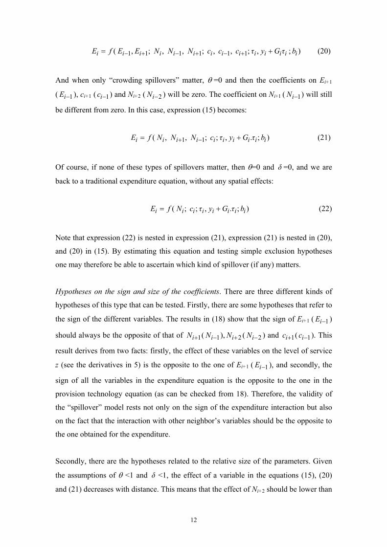
And when only “crowding spillovers” matter, θ =0 and then the coefficients on Ei+1

( 1−iE ), ci+1 ( 1−ic ) and Ni+2 ( 2−iN ) will be zero. The coefficient on Ni+1 ( 1−iN ) will still

be different from zero. In this case, expression (15) becomes:

);.,;;,,( 11 iiiiiiiiii b τG y τ c N N N fE += −+ (21)

Of course, if none of these types of spillovers matter, then θ=0 and δ =0, and we are

back to a traditional expenditure equation, without any spatial effects:

);.,;;( iiiiiiii b τG y τ c N fE += (22)

Note that expression (22) is nested in expression (21), expression (21) is nested in (20),

and (20) in (15). By estimating this equation and testing simple exclusion hypotheses

one may therefore be able to ascertain which kind of spillover (if any) matters.

Hypotheses on the sign and size of the coefficients. There are three different kinds of

hypotheses of this type that can be tested. Firstly, there are some hypotheses that refer to

the sign of the different variables. The results in (18) show that the sign of Ei+1 ( 1−iE )

should always be the opposite of that of 1+iN ( 1−iN ), 2+iN ( 2−iN ) and 1+ic ( 1−ic ). This

result derives from two facts: firstly, the effect of these variables on the level of service

z (see the derivatives in 5) is the opposite to the one of Ei+1 ( 1−iE ), and secondly, the

sign of all the variables in the expenditure equation is the opposite to the one in the

provision technology equation (as can be checked from 18). Therefore, the validity of

the “spillover” model rests not only on the sign of the expenditure interaction but also

on the fact that the interaction with other neighbor’s variables should be the opposite to

the one obtained for the expenditure.

Secondly, there are the hypotheses related to the relative size of the parameters. Given

the assumptions of θ <1 and δ <1, the effect of a variable in the equations (15), (20)

and (21) decreases with distance. This means that the effect of Ni+2 should be lower than

13

that of Ni+1 and the effect of ci+1 should be lower than the effect of ci. In fact, the ratio

between the different lags of a variable provide information about the magnitude of the

spillover. In equation (15), the ratio between the effects of ci+1 (ci-1) and ci provides an

estimate of the “benefit spillover” parameter θ :

Ω/Ω/

//

// 11

φτzφτzθ

cEcE

cEcEθ

iC

iC

ii

-ii

ii

ii−−

=∂∂∂∂

=∂∂∂∂

= + (23)

And onceθ has been obtained, δ can also be identified from the effects of Ni+1 (Ni-1)

and Ni+2 (Ni-2):

λθθλδ−

= where δθ

θδφτδθz

φθδτzNENE

NENEλ

iN

iN

-ii

-ii

ii

ii+

=+−

−=

∂∂∂∂

=∂∂∂∂

=+

+Ω/)(

Ω///

//

1

2

1

2 (24)

Since we have assumed that both θ and δ are lower than one, a check of this condition

will also provide a reliability test of our model’s validity.

In equation (21), the ratio between the effects of ci+1 (ci-1) and ci also provides an

estimate of the “benefit spillover” parameter θ . In this case, however, there is one

additional hypothesis to test, since this ratio should be equal to the ratio between the

effects of Ni+1 (Ni-1) and Ni:

N

N

ii

ii

ii

ii

C

C

ii

ii

ii

iizθz

NENE

NENE

zθz

cEcE

cEcEθ =

∂∂∂∂

=∂∂∂∂

==∂∂∂∂

=∂∂∂∂

= −+−+/

//

//

//

/ 1111 (25)

In equation (17), the ratio between the effects of Ni+1 and Ni provides an estimate of the

“crowding externalities” parameter δ :

N

N

ii

ii

ii

iizδz

NENE

NENEδ =

∂∂∂∂

=∂∂∂∂

= −+/

//

/ 11 (26)

Thirdly, note that the absolute size of the coefficients of the lagged variables increase

with the size of the “spillover” parameters θ and δ . For example, it is clear that the

14

coefficients of Ei+1 ( 1−iE ) and ci+1 ( 1−ic ) grow with θ , and that the coefficients of Ni+1

( 1−iN ) and Ni+2 ( 2−iN ) grow both with θ and δ . If one is able to break the sample of

municipalities according to a given rule that identifies two groups of municipalities, one

more sensible than the other to the effects of “spillovers”, then one would expect higher

coefficients for the neighbors’ variables in the first group that in the second one.

The way to test our model will therefore consist of various steps. Firstly, we will

estimate the equations in (15), (20), (21) and (22) and will test the different exclusion

hypotheses involved. Secondly, we will look at the sign of the different variables and

check whether they correspond to those expected. Thirdly, once the correct spillover

model has been selected, we will check the robustness of the model with regard to the

predictions on the relative magnitude of the parameters, and we will obtain estimates for

the two spillover parameters in order to check that they are indeed lower than one.

Finally, we will re-estimate our equations for several sub-samples of local governments

(i.e., rural and urban, suburbs and city centers), grouped according to the expected

relevance of the spillover phenomenon.

3. Empirical evidence

3.1 Empirical model

The theoretically-derived equation in (15) is approximated by a linear relationship

between spending and its determinants. In order to prevent problems of

heteroscedasticity and multicollinearity, we used per capita spending instead of total

spending. For the same reason, we used the ratio between first and second order

neighbors’ population and own population –instead of neighbors’ population–, and we

substituted the tax-share τi by the tax-price ti –computed as the product of the tax-share

τi and 1/Ni–, including also the squared of the population in the equation5. Taking all

these aspects into consideration, the estimated equation is:

5 Note that, after this transformation, the own population coefficients do not pick only the effect of population on the level of service (i.e., congestion effect) but also its effect on the tax bill.

15

iiiii

iiiiiiiiii

bαtgαyαtα

cαcαNNαNNαNαNαeαe

... . .

W. .)/K.()/K.(..W.

111098

762542

321

++++

++++++= (27)

where ei is per capita spending, Wei is first-order neighbors’ per capita spending, iN

and 2iN are the population and its squared, ii NN /K and ii NN /K2 are the ratios

between first-order and second order neighbors’ population and own population, ci is a

cost variable and Wci measures first-order neighbors’ costs, ti is the tax-price, yi is per

capita income, giti is the product of per capita grants (gi) and the tax-price6, and bi are

preference variables.

W and K are J×J matrices that identify which are the first-order neighbors of each

municipality, with J being the number of municipalities in the sample. The only

difference between matrices W and K is that W is row standardized and K is not. This

means that Wei and Wci should be interpreted as the average of per capita spending and

costs, respectively, of the municipalities considered as first-order neighbors, while iNK

is the sum (not the average) of the population of the municipalities considered as first-

order neighbors. 2K is a non-standardized J×J matrix identifying second-order

neighbors’, so iN2K is the sum of the population considered to be second-order

neighbors7. Note that, since spending is expressed in per capita terms, it would have no

sense to compute neighbors’ spending as a sum of per capita spending of several

municipalities. This argument does not apply to neighbors’ population since, in this

case, theory suggest that the magnitude of “crowding externalities” depends on the head

count of the population living in the neighborhood.

This slightly different specification does not alter the procedure presented in the

previous section to test the exclusion hypotheses and the hypotheses regarding the sign

of the variables. However, the hypotheses regarding the relationship between the size of

the population parameters and distance cannot be tested directly, and a computation of

6 Note that this is equivalent to multiply the overall amount of grants by the tax-share (giti= Giτi). 7 We delay to section 4.2 the explanation of the way used to compute these matrices.

16

the derivatives of Ei with respect to iN , iNK and iN2K based on the results of (27) is

needed.

3.2. Local governments in Spain

The hypotheses developed above will be tested using data on a cross-section of Spanish

local governments. Spanish municipalities have spending responsibilities similar to

those in other countries (e.g., water supply, refuse collection and treatment, street

cleaning, lighting and paving, parks and recreation, traffic control and public

transportation, social services, etc) with the only exception of education, that is a

responsibility of regional governments in Spain. Unfortunately, we did not have access

to spending data for each service, so our analysis will be confined to overall spending,

leaving detailed service analysis for future work.

Despite of this, we consider that Spain is a good testing ground for our theory, for three

different reasons. First, the local layer of government in Spain is highly fragmented.

Spain has more than 8,000 municipalities, most of them quite small. This fragmentation

is not only a rural phenomenon but also an urban one. For example, the metropolitan

area of Barcelona (the second city of the country) has more than 100 municipalities.

Second, in Spain there are not effective supra-municipal service provision bodies.

Regional governments in Spain are quite active, but its geographical area is much

bigger than the typical urban agglomeration, metropolitan governments are absent8, and

voluntary agreements between municipalities are residual or quite ineffective. Third,

these services are financed mainly from taxes and unconditional grants. User charges

are also relevant, but they use to be much lower than provision costs in most services

(e.g., cultural and sports facilities) or can not be charged in others (e.g., parks).

Moreover, tolls are practically inexistent and parking charges are still below the

efficient levels. Unconditional grants do not compensate municipalities for the costs

created by visitors, and there are very few matching grants that could be considered as

an externality-correcting device.

8 The only remarkable attempt to build a metropolitan government occurred in the urban metropolitan area of Barcelona during the 80’s (known as “Corporación Metropolitana de Barcelona”), but this institution was banned by a law of the regional government and its main responsibilities (water transportation and treatment, and public transportation) assigned to two different public agencies.

17

3.3. Data and variables

Equation (27) will be estimated using data on 2,610 Spanish municipalities during the

year 1999. The budget data comes from a survey on municipal finances undertaken by

the Ministry of Economics. Most municipalities with a size higher than 20,000

inhabitants are included in the survey. The survey selects a representative sample for

municipalities below this population threshold. However, we had to exclude

municipalities with less than 1,000 inhabitants because of a lack of income and tax-

price data.

The dependent variable is current spending per capita. Spending has been computed

from data on municipal outlays, and includes data on wages and salaries, purchases and

transfers. Apart from population, we also include a cost measure, personal income, tax-

price, grants and preference variables in the equation. The cost variable (c) has been

constructed by multiplying average per capita spending in the sample and a cost index,

computed from a set of variables that are available for our sample of municipalities and

which have been used in previous analysis of local government costs in Spain (Solé-

Ollé [34]; Bosch and Solé-Ollé [7]): urbanized land area per capita (Land), wage rate in

the service sector (Wage), unemployed (%Unemployed), non-EU immigrants

(%Immigrants)9, and an index of service responsibilities (Responsibilities). The variable

Land accounts for the effects of urbanization patterns on costs. The variable Wage rate

measures input costs10. The variables %Unemployed and %Immigrants measure the

effects of density related to poverty and the harshness of the environment (Rothenberg

[32]). In order to compute the index of service responsibilities (Responsibilities) we

used information on spending per head in the various expenditure programs for the

municipalities of one of the main regions of the country (Catalunya). This information

comes from a special survey carried out by a higher-tier of local government

(“Diputación de Barcelona”) in order to compute the amount of spending due,

respectively, to compulsory and non-compulsory responsibilities. With this information

we are able to compute the average expenditure per capita in the additional

9 The definition, statistical sources and descriptive statistics of the variables are presented in Table 1. 10 Unfortunately, wage information is not available at municipal level, and has been computed using provincial data. Given that labor markets are usually much bigger than municipalities this need not be a limitation.

18

responsibilities that municipalities are obliged by law to provide when they surpass the

5,000, 20,000 and 50,000 population thresholds11. All these variables have been

aggregated into a single cost index using the coefficients obtained by Bosch and Solé-

Ollé[7] for each of them as weights12. This procedure has the advantage of producing a

more parsimonious equation to estimate, especially in the case of benefit spillovers,

since all the cost variables (if entered alone) should be accompanied by the

corresponding first-order neighbor’s cost variables13.

The tax-price measure (ti) aims to reflect the high degree of tax exporting in the Spanish

case. The three main municipal taxes in Spain are the property tax, the business tax and

the motor vehicle tax. In the case of the property tax, the burden of the tax falls partly

on non-residents who own houses in the municipality, and partly on the owners of

business property. The degree of tax exporting of the business tax is even higher. In the

case of companies, the full amount of the tax is probably exported, and in the case of

individual owners (e.g., small shops) they can hardly be considered to be the median or

representative voter of the municipality. Something similar happens with the motor

vehicle tax, since the burden falls partly on the business sector (e.g., trucks, vans, car

renting). To account for these tax-exporting possibilities, the tax-price is measured as

the ratio between the tax bill of a representative resident in those three taxes and per

capita tax revenues in the municipality. The tax bill of a representative resident is

computed as the sum of the property tax per urban unit divided by the average size of an

11 The increases in expenditure at these thresholds are of 6.5, 1.97 and 1.66 per cent, respectively, meaning that our responsibility index takes the value of 1 if the population is lower than 5,000, the value of 1.065 if the population is higher than 5,000 but lower than 20,000, the value of 1.085 if the population is higher than 20,000 but lower than 50,000, and the value of 1.101 if the population is higher than 50,000. 12 Bosch and Solé-Ollé [7] estimate a log-linear expenditure equation that allows for identification of the parameters of these variables in the cost function. Some of the variables are measured in logs, so the cost function is multiplicative: constant × Wagei

0.7 × Responsibilitiesi ×Landi0.05× exp(2×% Unemployedi) ×

exp(1.2×%Immigrantsi). The constant of the cost function can not be identified, so costs have to be measured in relative terms, with an index computed by multiplying the above expression by the population, dividing by the summation of the results across all the municipalities of the sample, and dividing again by the population share of the municipality. See Solé-Ollé [34] and Bosch and Solé-Ollé [7]. 13 However, this two-step procedure may also introduce some biases into the estimation. To check this possibility, we have also the extended version of the model, with each cost variable entering separately and including also the neighbors’ variables. The results of both procedures are qualitatively similar, with all the cost variables having a positive impact on expenditure, but the standard errors are higher in the second one. These results are available from the author.

19

urban unit in the sample, and the motor vehicle tax per vehicle divided by the average

number of vehicles per capita in the sample. Note that the business tax does not appear

in the numerator; we assume that the representative resident is not a business owner.

Variation in our tax-price measure is high, ranging from 0.2 to 0.8, which is due mostly

to the fact that the business tax base is distributed very unevenly across municipalities14.

The income variable (yi) is personal income per capita in the municipality, since we

have not been able to measure the income of the median voter. The variable that

measures current grants per capita received by the municipality (gi) includes the main

unconditional transfer received from the central government (“Participación de los

Municipios en los Ingresos del Estado”) and other minor transfers. This variable has

been multiplied by the tax-price (giti). We include two variables in order to measure the

resident’s preferences for public goods (bi): the shares of population older than 65 and

younger than 18.

Finally, we included a set of fifty provincial dummies in order to account for

unobserved effects common to all the municipalities belonging to the same province.

However, according to the results of a Wald test, these dummies were not jointly

significant and we decided to drop them from the equation.

3.4. Econometric issues

In this section, we deal with the two main econometric problems that we encounter in

the estimation of equation (27): the definition of neighboring municipalities and the

endogeneity of neighbors’ expenditure in the benefit spillovers model.

The first econometric problem concerns the way the neighbors of a municipality are

defined. Identification issues allow neither the inclusion of tax interactions for each pair

of municipalities, nor of the average value of the sample. Instead, an ‘a priori’ set of

interactions has to be defined and tested. However, as Anselin [1] notes, there is some

14 The measure of the tax price could be improved with information on the share of the property and vehicle taxes paid by the business sector. Unfortunately, this information is not available in our case. However, we feel that our measure a considerable proportion of the variation in the tax price that can be attributed to tax exporting.

20

arbitrariness in the definition of these interactions. It is wise therefore to rely, when this

is possible, on insights derived from the theoretical model and on auxiliary evidence.

Our model suggests that interactions are derived from expenditure spillovers. Moreover,

given the nature of local public services, the channel of transmission of these spillovers

is the mobility of residents, which depends heavily on the distance between

municipalities. The theoretical model suggests also that the expenditure equation should

include first-order neighbors’ spending and costs, and first and second-order neighbors’

population. It is not clear, however, how these first and second order neighbors should

be defined. In fact, we could have included second-order neighbors directly in equations

(1) and (3), which define how the benefit and crowding spillovers operate. In this case,

the expenditure equation should include first and second order neighbors’ spending and

cost variables, and up to fourth-order neighbors’ population. The conclusion is that the

number of lags for the population always should be twice the number of lags for

spending and cost variables.

This suggests that we have to decide which radius defines first and second order

neighbors, and which number of lags should be included in each of the neighbors’

definitions. Daily mobility patterns in Spain may help us to take these decisions. We

know, for example, that in the metropolitan area of Barcelona (the second biggest city in

Spain) people travel an average distance of 18.1 Km15. Moreover, 81% of these

journeys are of distances of less than 20 Km and 92% are of distances of less than 30

Km. As a result of this evidence, we decided to use only one lag and to define first-

order neighbors as the municipalities located less than 30 Km away, and second order

neighbors as the municipalities located between 30 and 60 Km away16. In order to

account for the fact that the effect of spillovers decays with distance inside this radius,

we use inverse distance weights. The matrices K and K2 of equation (27) have elements

kij and k2,ij:

15 Enquesta de mobilitiat quotidiana de la Regió Metropolitana de Barcelona, 2001. This mobility includes all the different modes (job, studies, shopping, etc.) and means (private and public). 16 We also performed the analysis with radiuses of 20 and 40 Km (instead of 30 and 60 Km). We also performed the analysis with two of first-order neighbors (15 and 15 to 30 Km) and two of second-order neighbors (30 to 45 Km, and 45 to 60 Km). In all cases, the results were very similar to those presented in this paper and are available from the author.

21

⎪⎩

⎪⎨⎧ ≤<=

otherwise 0Km 300 if/1 d dk ij

αijij and

⎪⎩

⎪⎨⎧ ≤<−=

otherwise 0 Km 60 Km 30 if )30/(1k ,2

ijijij

dd α

where dij is the distance between municipalities i and j. We tried different values for α,

between 0 and 2, but α=0.5 performed better than the others. These two matrices are not

row standardized, contrary to what is usual in the spatial econometrics literature

(Anselin [1]). The reason of this is that they are used only to compute neighbors’

population and, according to the theory these variables should enter in the equation as

the head count of the population residing in the neighborhood and not as the average of

the population size of neighbor municipalities.

The matrix W of equation (27), used to compute first-order neighbor variables for per

capita spending, is simply the matrix K row-standardized. The reason for row-standardi-

zation in this case is that it would have no-sense to compute the sum of several per

capita spending or cost variables. That is, matrix W has elements ij w computed as:

⎪⎩

⎪⎨⎧ ≤<∑=

otherwise 0Km 300 if)/1/()/(1 d dd w ijj

αij

αij

ij

Note that the use of distance-based weights in the computation of both K and W has

implications for the interpretation of the effects of spatially lagged population, since the

effect of increasing the number of inhabitants in the a municipality on spending done in

another one depends on the distance between these two municipalities. So, for example,

the effect of an increase in the population of a first-order neighbor j and a second-order

neighbor l on i’s spending can be approximated by:

5.0411

ijj

ij

j

id

αNNeβα

NE

⎟⎟⎠

⎞⎜⎜⎝

⎛+−=

∂∂ and 5.05

)30(1−

=∂∂

ijl

i

dNE

α , where ∑

=j

5.011

ij/dβ (28)

22

The second econometric problem refers to the endogeneity of Wei in equation (27):

expenditure in municipality i depends on expenditure in j, but expenditure in j also

depends on expenditure in i. In order to obtain consistent estimates of the expenditure-

interaction parameter, a simultaneous estimation procedure is therefore required. The

available procedures are either maximum-likelihood (Anselin [1]) or instrumental

variables. I use the latter approach, following the practice of a number of papers in the

policy-interactions literature (Besley and Case [5]; Figlio et al. [18]; Brett and Pinske

[11]; Buettner [14]; Baicker [4]). As is standard in this literature, the instruments used

will be some of the determinants of neighbors’ expenditure: first-order neighbors’ tax-

price Wti, personal income per capita Wyi, current grants Wgi ×ti, share of old

population Wpoi, and share of young population Wpyi17. Since the first-order spatial

lags sufficed to explain a considerable portion of neighbors’ spending variation in the

first-stage regression18, we decided not to use further spatial lags of these variables to

prevent over-fitting bias (Staiger and Stock [36]). Moreover, the results of the Sargan

test suggested that these instruments are not correlated with the error term and are,

therefore, valid.

Instrumental variable estimation has the added advantage of ensuring that the

correlation in the level of spending is not due to common shocks, since IV estimates are

consistent even in the presence of spatial error autocorrelation (as Kelejian and Prucha

[25] demonstrate). However, in the case of spatially autocorrelated error terms (i.e.,

ititit u+= ελε W ), estimates are no longer efficient. To check this possibility, I have

used the Anselin and Kelejian [2] version of the Moran’s test, which is suitable for

testing for spatial autocorrelation in the presence of endogenous regressors. I computed

this statistic using both the W and W2 weights matrices. Although it is not possible to

rule out that there is some autocorrelation in the residuals in the expenditure equations

without spatially lagged variables, this autocorrelation disappears in the different

models that include either the spatially lagged dependent variable or the spatially lagged

17 Note that neighbor’s population and costs can not be used as instruments since theory tells us that they should be included as explanatory variables in the expenditure equation. 18 The F-statistics on the statistical significance of the instruments in the first-stage equation are always higher than 20, which exceeds the rule-of-thumb of 10 suggested by Staiger and Stock[36]. So we must conclude that our instruments are no weak.

23

population. These results suggests that our IV results are both consistent and efficient

and that more sophisticated procedures as the GMM method proposed by Kelejian and

Prucha [25] will not improve them.

3.5. Results

The results of the estimation of the different models are presented in Tables 2 and 3.

Table 2 presents the results of the estimation of different specifications with the full

sample of 2,610 municipalities. The results of column (a) of Table 2 correspond to the

No-spillovers model (expression 22) and show that the different control variables

introduced in the equation are able to account for a sizeable proportion of local spending

variation (roughly 50%). Moreover, most of these variables are statistically significant

and have the anticipated signs, with the proportion of young population being the sole

exception to this rule. Local spending decreases and then increases with population.

Local spending is higher as production costs increase, and the lower the tax-price, the

higher the personal income and transfers received, and the lower the share of old

population. All these results are consistent with previous analyses of local spending in

Spain (Solé-Ollé [34], and Bosch and Solé-Ollé [7]). However, it is unclear whether this

is the appropriate model, since the results of the Moran tests suggest that there is spatial

correlation in the error terms, both with the first and second-order neighbors’ matrices.

This suggests a possible omission of spatially correlated variables and the need to test

whether some of our spillover models are appropriate.

The results of columns (b) to (e) correspond to the Benefit + Crowding spillovers

model. The OLS results of column (b) suggest positive interactions between the

spending of neighboring municipalities and a positive effect of first and second order

neighbors’ populations, although these last two coefficients are not statistically

significant. The effect of neighbors’ costs, contrary to our expectations, is negative and

not statistically significant. Things do not improve when second order neighbors’

spending and costs and third order populations are added (column (c)), meaning that the

problem does not seem to lie in the appropriate distance decay for these variables. When

we re-estimate by Instrumental Variables, the results greatly improve –see the results of

24

column (d) and note that we still obtain statistically significant spending interactions,

although the sign is now negative. The results of the Sargan test at the bottom of the

table suggest that the instruments we have used in the estimation are valid19. Moreover,

the neighbors’ cost index now has a positive and significant effect on spending, as

suggested by our theoretical model. The results of column (e) tell us that while second

order neighbors’ population does have an effect on spending, this is not true of second

order spending and costs, and of third order neighbors’ populations. Note that these

results are fully consistent with the exclusion hypotheses presented in the theoretical

section.

In order to check the robustness of these results we show in columns (f) to (h) the

estimation of three alternative specifications. The results shown in column (f)

correspond to the Benefit spillovers model (expression 20). The only difference of this

specification is the exclusion of the second order neighbor’s populations. The OLS

results are omitted to save space. The IV results are similar to the previous ones (see

column (d)), with the relevant coefficients of the same sign and magnitude. However,

the explanatory capacity of the model drops a little bit and the t-statistic clearly suggests

that second order neighbor’s populations can not be excluded from the equation. The

results in column (h) correspond to the Crowding externalities model (expression 21)

The only differences between this specification and the full model (column (d)) is the

exclusion of neighbor’s spending and costs. The results are quite similar to those of the

full model, with first and second order neighbor’s populations having a positive and

significant impact on spending. However, the results suggest that also in this case is not

possible to exclude neighbor’s spending and costs. Finally, column (h) shows the results

of the Spending Interactions model. This specification does not correspond to any of the

equations developed in the theoretical section. However, we have decided to show the

results of this equation to allow the comparison of its performance with the other

equations estimated, given that this is the specification used in previous studies (e.g.,

19 Given the high magnitude of the OLS bias implied by change in the sign of the interaction, we wondered if these results were driven by any of the instruments we used. To check this possibility we reestimated by IV excluding the instruments one-by-one and using a “differences-in-Sargan” statistic (Hayashi [24]) to test for the validity of each instrument. This statistic has been computed as the difference of the Sargan statistics of the equations excluding and including the suspicious instrument, and is distributed as a χ2(K) with K=loss of over-identifying restrictions. All the instruments were valid and the results obtained when excluding one of them were not qualitatively different.

25

Case et al. [15] and Baicker [4]). We also omit here the OLS results and go directly to

the IV ones, that show that the neighbor’s spending coefficient is no longer statistically

significant, while the OLS results (not included here) showed a positive and significant

coefficient (as in the other OLS results with neighbor’s spending included in Table 2).

Note also that the Moran’s I statistic suggest both first and second order residual spatial

correlation. Therefore, we should conclude that the Spending Interactions model is not

the appropriate one.

The check on exclusion constraints presented in the previous section thus suggests that

the correct model for including the effects of spillovers is the Benefit + Crowding

spillovers model, which accounts simultaneously for spending interactions and for the

effects on local spending of first-order neighbors’ costs and first and second-order

neighbors’ populations. We can check the robustness of the results by analyzing the

additional hypothesis regarding the sign and the relative size of the coefficients

developed in the previous section. Firstly, note that, as expected, the sign of the

neighbors’ spending is negative while that of the neighbors’ cost index is positive.

Second, the effect of the own cost variable is much higher than the effect of neighbors’

costs, as the model suggested. Moreover, we could use expression (28) to compute the

derivatives of Ei with respect to first and second-order neighbor’s population. Since

these derivatives are, however, contingent on the distance, we compute them at different

distances (i.e, 1Km, 7.5 Km, 15 Km and 30 Km) using the mean sample values of the

different variables involved20. The values we get for ji NE ∂∂ / are 20.38 (1 Km), 7.44

(7.5 Km), 5.26 (15 Km) and 3.72 (30 Km) and the value we get for li NE ∂∂ / at 30 Km

is 1.016. Note that by construction, the effect of first-order population is decreasing in

distance. In any case, however, the effect of first-order population at 30 Km is three to

four times the effect of second-order population at this distance.

Finally, we can use expressions (23) and (24) to compute the Benefit and Crowding

spillovers parameters, respectively. In this case, these parameters take the values of

θ =0.33 and δ =0.059 and are statistically significant at the 95% level (see Table 4 for a

20 The values used for the parameters of expression (28) are: α1=0.213 (see Table 2), β=1/7.82 (with an average distance between municipalities of 10.1 Km and an average number of 36 neighbors per municipality), ej=326 (see Table 1), Ni/Nj=2,134, α4=1.433 and α5=1.016.

26

summary of the values of these parameters for different samples)21. Spillovers therefore

not only seem to be relevant, but they are also sizeable. One Euro of local spending

provides the same utility to a typical resident as three Euro of neighbors’ spending, and

an additional non-resident living 30 Km away leads to the quality of public services in

the locality decreasing less than ten times less than an additional resident would.

Table 3 presents the results obtained when breaking the sample into Urban and Non-

Urban municipalities, and when considering the Suburbs and the City centers

separately. There are two intuitions behind this analysis. The first intuition is that if

spillovers arise because of the daily mobility of citizens between municipalities, they

should be more pronounced in large urban areas, where mobility is also more relevant.

The second intuition is that in urban areas, Benefit spillovers may be more prevalent in

the Suburbs, and Crowding externalities may be more important in City centers. This is

because City centers are much bigger than Suburbs and play a prominent role as

employment and administrative centers. City centers therefore usually experience a net

inflow of population while Suburbs usually experience (on average) a net outflow. It is

therefore to be expected that residents in the Suburbs tend to benefit more from the

services provided in other localities than City center residents and, at the same time, we

can expect also that the services in the City centers are more crowded by non-residents

than the services in the Suburbs.

To test these hypotheses, we divided our sample into Urban and Non-Urban areas. In

line with previous analyses, urban municipalities were defined as those located less than

35 Km from a city center with more than 100,000 inhabitants (Solé-Ollé and Viladecans

[35]). Using this procedure, we are able to identify 36 large urban areas that contain

1,259 Suburbs and 36 City centers. We therefore have 1,315 Non-Urban and 1,295

Urban municipalities. The results of Table 3 show important differences between

Urban and Non-Urban municipa-lities. The results for the Urban municipalities

(columns (a) and (b)) are similar to those presented for the full sample (see Table 2),

21 Standard errors have been computed using the formula for the variance provided in Theorem (ii) of Chapter (vi) of Rao [31], which can be expressed as ∑ ∂∂∂∂= i jiijE aχaχνs )/)(/(2 , where ),( δθχ ≡

is the vector of structural parameters and )/,/,/,/( 211 +++ ∂∂∂∂∂∂∂∂≡ NENEcEcEa is the vector of estimated coefficients.

27

since both Benefit and Crowding spillovers matter. However, the size of the coefficients

for the neighbor’s variables is now bigger than before, suggesting that spillovers are of a

higher magnitude. This intuition is confirmed by the identification of the two spillover

parameters, since we found that θ =0.67 and δ =0.24. These coefficients are

statistically significant at the 95% level (see Table 4). It should be remembered that

these parameters were 0.33 and 0.059 for the full sample. The results for the Non-urban

municipalities (columns (c) and (d)) are similar, but the size of the neighbors’

coefficients is lower and some of them are not statistically significant (second-order

population) or only statistically significant at the 90% level (first-order neighbors’

spending and costs). The value of the spillover coefficients is now much lower, since

we found that θ =0.14 and δ =0.04, but these coefficients are not statistically

significant at conventional levels (see Table 4). We can conclude, therefore, that

spillovers are more relevant in Urban than in Non-Urban areas, as expected.

The results of Table 3 also show significant important differences between Suburbs and

City centers. The results for the Suburbs (columns (e) and (f)) are virtually the same as

for the full sample of Urban municipalities. The results for the City centers are

different. Both first-order neighbors’ spending and costs are not statistically significant,

suggesting that Benefit spillovers are not present, and that only Crowding externalities

are relevant. The fact that second-order neighbors’ populations have a positive and

statistically significant effect does not necessarily contradict this statement, since it may

simply mean that the distance decay function may be different for City centers than for

Suburbs. The identification of spillover coefficients confirms these conclusions. For the

Suburbs, we found that θ =0.69 and δ =0.27 while for City centers, we found that θ =0

and δ =0.4622. The coefficients are statistically significant at the 95% level for Suburbs

but in the case of City centers only the δ coefficient is statistically significant at the 90%

(see Table 4). These results confirm our expectations. We admit, however, that the

results for City centers should be taken with caution, given the small number of

observations involved and the lower explanatory power of the expenditure equation.

22 Given that θ=0, in this case we made use of expression (26) to identify δ, using the expression ∂Ei/∂Ni=(α2Ni-2α3Ni

2)+ei.

28

4. Conclusion

The simple model sketched in this paper allowed us to test for the presence of

spillovers, confirming that this is a relevant problem in Spain, and that this problem is

more acute in Urban areas than in the rest of the country. The model allowed us to

differentiate between different types of spillovers. We showed that two different kinds

of spillovers (Benefit spillovers and Crowding externalities) should be taken into

account in this kind of analysis. Failure to account for one of these types of spillovers

leads false inferences being drawn, suggesting either that spillovers are present when

they are not or that they are not relevant when they are. Both kinds of spillovers are

important in the Suburbs but only one type (Crowding externalities) is relevant in City

centers. The model also allowed us to obtain an estimate of the size of each type of

spillovers. These results suggest that spillovers are not only present but also are of a

considerable magnitude, especially in Urban areas. The magnitude of the inefficiencies

(and inequities) associated with these spillovers should therefore be a concern for

policy-makers.

However, we have to admit that the approach used in the paper may have at least two

fundamental weakness that merit some further comments. First, it can be argued that the

expenditure interactions generated by the model may also arise as a result of alternative

behavioral models. For example, as Brueckner [12] points out, interactions between

local governments may also be predicted by the standard tax competition model

(Brueckner and Saavedra, [13]). Note however that, although the model has not been

designed to provide a test against other competing hypotheses, it provides a set of

predictions that must be fulfilled by the empirical results in order to accept the spillover

story is plausible. These hypotheses refer not only to the statistical significance of

spatially lagged expenditure, as in previous analyses (Case et al. [15]), but also to the

inclusion of other neighbors’ covariates, and to the sign and size of the coefficients of

the different variables. Moreover, household fiscal mobility is not seen as a tight

constraint on the operation of local governments in Spain. This is the result of the

limited scope of Spanish local governments, which do not provide the services that

cause the mobility experienced in other countries (e.g., education in the US).

29

Second, one may wonder to what extent the fiscal interactions identified are driven by

the operation of matching grants, user charges, or any other fiscal instruments designed

to deal with the externalities, instead of being the result of the reaction of local

governments to the spillover’s problem. But as we have argued in section 4.2, Spanish

local governments make little use of most of the instruments that use to be

recommended to internalize these externalities. And, in any case, if these instruments

where used effectively we should observe no interactions between the fiscal choices of

neighboring municipalities. Note that, instead of this, we have found evidence of

sizeable spillovers. If externality-correcting instruments were present but not fully

effective, then the estimated magnitude of the spillovers obtained in the paper should be

considered a lower bound of its real value.

Therefore, although we acknowledge that further efforts to explicitly test our hypothesis

against competing ones are necessary, we therefore consider that the results provided in

this paper show some preliminary evidence in favor of our model.

30

References

Anselin, L.. Spatial econometrics, methods and models. Kluwer Academic. Dordrecht

1988.

Anselin, L., and Kelejian, H.. Testing for spatial autocorrelation in the presence of

endogenous regressors. International Regional Science Review 20 (1999) 153-

182.

Arnott, R. and Grieson, R.E.. Optimal fiscal policy for a state or local government.

Journal of Urban Economics 9 (1981) 23-48.

Baicker, K. The spillover effects of state spending. Journal of Public Economics 89 (2-

3) (2005) 529-544.

Besley, T. and Case, A.. Incumbent behaviour, vote-seeking, tax setting and yardstick

competition. American Economic Review 85 (1995) 25-45.

Borcherding, T.E. and Deacon, R.T.. The demand for the services of non federal

governments. American Economic Review 62 (1972) 891-901.

Bosch, N. and Solé-Ollé, A. On the Relationship Between Authority Size and the Costs

of Providing Local Services: Lessons for the Design of Intergovernmental

Transfers in Spain. Public Finance Review 33 (2005) 318-342.

Boskin, M.J.. Local government tax and product competition and the optimal provision

of public goods. Journal of Political Economy (1973) 203-210.

Brainard, W. and Dolbear, F.T.. The possibility of oversupply of local ‘public’ goods, a

critical note. Journal of Political Economy 75 (1967) 86-90.

Bramley,G.. Equalization grants and local expenditure needs. Avebury, England 1990.

Brett, C. and Pinske, J.. The determinants of municipal tax rates in British Columbia.

Canadian Journal of Economics 33 (2000) 695-714.

31

Brueckner, J.K.. Strategic interactions among governments; an overview of the

empirical literature. International Regional Science Review 26(2) (2003) 175-

188.

Brueckner, J.K. and Saavedra, L.A.. Do local governments engage in strategic property

tax competition?. Journal of Urban Economics 54 (2001) 203-229.

Buettner, T.. Local business taxation and competition for capital, the choice of the tax

rate. Regional Science and Urban Economics 31(2-3) (2001) 215-245.

Case, A.C., Hines, J.R. and Rosen, H.S.. Budget spillovers and fiscal policy

interdependence, evidence from the states. Journal of Public Economics 52

(1993), 285-307.

Conley, J. and Dix, M.. Optimal and equilibrium membership in clubs with the presence

of spillovers. Journal of Urban Economics 46 (1999) 215-229.

Dalhby, B.. Fiscal externalities and the design of intergovernmental grants.

International Tax and Public Finance 3 (1994) 397-412.

Figlio, D.N., Kolpin, V.W. and Reid, W.E.. Do states play welfare games?. Journal of

Urban Economics 46 (1999) 437-454.

Furlog, W.S. and Mehay, S.L.. Urban law enforcement in Canada, an empirical

analysis. Canadian Journal of Economics 14 (1981) 44-57.

Gordon, R.H.. An optimal taxation approach to fiscal federalism, Quarterly Journal of

Economics, 98 (1983) 567-86.

Greene, K.V., Neenan, W.B. and Scott, C.D.. Fiscal interactions in a metropolitan

area. Lexington Books, Lexington 1977.

Hakim, S.A., Ovadia, E.S. and Weinblatt, J., Interjurisdictional spillovers of crime and

police expenditure, Land Economics (1979) 100-12.

Haughwout, A.K.. Regional fiscal cooperation in metropolitan areas, an exploration.

Journal of Policy Analysis and Management 18 (1999) 579-600.

32

Hayashi, F. . Econometrics 1st ed. Princeton University Press, Princeton, New Jersey

2000.

Kelejian, H.H. and Prucha, I.. A generalised spatial two-stage lest squares procedure for

estimating a spatial autoregressive model with autoregressive disturbances.

Journal of Real Estate Finance and Economics 17 (1998) 99-121.

Ladd, H.F. and Yinger, J.. American ailing cities, fiscal health and the design of urban

policy. The Johns Hopkins University Press, Baltimore & London, 1989.

Le Grand, J.. Fiscal equity and central government grants to local authorities. Economic

Journal 85 (1975) 531-47.

Murdoch, J., Rahmatian, M. and Thayer, M.. A spatially autoregressive median voter

model of recreation expenditures. Public Finance Quarterly 21 (1993) 334-350.

Oates, W.E.. Fiscal Federalism. Harcourt Brace Jovanovich, New York, 1972.

Pauly, M.. Optimality, ‘public’ goods and local governments, a general theoretical

analysis. Journal of Political Economy 78 (1970) 572-585.

Rao, C.R. Linear statistical inference and its applications, Wiley, New York, 1965.

Rothenberg, J.. Poverty and urban public expenditures. Urban Studies 35 (1998) 1995-

2019.

Saavedra, L.A. A model of welfare competition with evidence from AFDC. Journal of

Urban Economics 47 (2000) 248-27.

Solé-Ollé, A. Determinantes del gasto público local: necesidades de gasto o capacidad

fiscal?. Revista de Economía Aplicada 25 (2001) 115-156.

Solé-Ollé, A. and Viladecans-Marsal, E.. Central cities as engines of metropolitan area

growth. Journal of Regional Science 44(2) (2004) 321-50.

Staiger, D. and Stock, J.H.. Instrumental variable regression with weak instruments.

Econometrica 5(65) (1997) 557-586.

33

Weisbrod, B.A. Geographic spillover effects and the allocation of resources to

education. Margolis, J. (Ed.): The public economy of urban communities.

Resources for the Future, Washington DC, 1965.

34

Table 1 Definition of the variables. Data sources and descriptive statistics

Variable 1999 Definition Data Sources Mean St. Dev.

current spending: ei Wages, supplies and current transfers

(outlays)

Ministry of Economics Municipal database

326.602 147.948

population: Ni Census of population National Institute of Statistics (INE)

13,540 73,358

cost index: ci Prepared by the author using data on wages,

land area, immigrants, unemployed, and responsibilities

Salary Statistics (INE), Property Assessment

Office, Census data (INE), Spanish Economic

Yearbook (‘La Caixa), and weights from Bosch

and Solé-Ollé [7]

327.511 621.241

tax-price: ti Prepared by the author using data on

population, urban units, number of vehicles, and

tax revenues

Ministry of Economics Municipal database, National Institute of

Statistics (INE), Property Assessment Office, Spanish Economic

Yearbook (‘La Caixa),

75.028 22.425

personal income per capita: yi Estimated personal income per capita

Spanish Economic Yearbook (‘La Caixa),

8.363 1.782

current grants per capita: gi × ti Current grants per capita multiplied by

tax-price

Ministry of Economics Municipal database

153.602 63.390

share old population: poi,t Population older than 65 over population

National Institute of Statistics (INE)

20.272 7.194

share young population: pyi,t Population younger than 18 over population

National Institute of Statistics (INE)

15.605 3.692

Notes: budgetary variables and income are measured in Euro; tax-price and population shares in %.

35

Table 2: Estimation of expenditure spillover models: Full sample (J = 2,610)

Variable No

spillovers Benefit + Crowding

spillovers Benefit

Spillovers Crowding spillovers

Spending interactions

(a) OLS (b) OLS (c) OLS (d) IV (e) IV (f) IV (g) OLS (h) IV

i) Neighbors’ variables

first-order spending: Wei --.-- 0.272 (5.045)***

0.255 (4.741)***

-0.213 (-2.918)***

-0.220 (-2.741)***

-0.224 (-3.018)***

--.-- -0.064 (-1.055)

second-order spending: W2ei --.-- --.-- 0.041 (0.897)

--.-- -0.046 (-0.631)

--.-- --.-- --.--

first-order cost index: Wci --.-- -0.077 (-0.354)

-0.076 (-0.320)

0.302 (2.882)***

0.562 (2.841)***

0.576 (3.074)***

--.-- --.--

second -order cost index: W2ci --.-- --.-- -0.000 (-0.013)

--.-- -0.032 (-0.069)

--.-- --.-- --.--

first-order population: KNi/Ni --.-- 0.913 (1.632)

1.021 (1.332)

1.433 (2.407)***

1.468 (2.369)**

1.861 (3.150)***

1.187 (2.054)**

--.--

second -order population: K2Ni/Ni--.-- 0.496

(1.532) 0.500

(1.641) 1.0

(3.147)*** 1.005

(3.056)*** --.-- 0.933

(2.501)** --.--

third -order population: K3Ni/Ni --.-- --.-- -0.154 (-0.368)

--.-- -0.058 (-0.621)

--.-- --.-- --.--

ii) Cost variables

population: Ni -0.175 (-3.658)***

-0.128 (-2.707)***

-0.125 (-2.723)***

-0.137 (-1.914)*

-0.141 (-1.900)*

-0.158 (-2.214)**

-0.132 (-2.869)***

-0.157 (-2.706)***

Population squared: Ni2 0.001

(1.745)* 0.001

(1.899)* 0.001

(1.745)* 0.002

(1.621) 0.002

(1.501) 0.002

(1.431) 0.001

(1.861)* 0.001

(1.786)*

cost index: ci 1.008 (6.618)***

0.915 (5.078)***

0.922 (5.112)***

0.919 (7.506)***

0.920 (7.435)***

0.915 (6.948)***

1.002 (6.555)***

1.005 (7.113)***

iii) Voter demand variables tax-price: ti -0.885

(-4.440)*** -0.712

(-3.392)*** -0.736

(-3.449)*** -0.899

(-6.361)*** -0.910

(-6.029)*** -0.923

(-6.655)*** -0.801

(-3.893)*** -0.924

(-4.269)***

personal income per capita: yi 0.027 (5.439)***

0.021 (5.111)***

0.025 (5.239)***

0.030 (5.529)***

0.032 (5.505)***

0.030 (5.489)***

0.027 (5.517)***

0.027 (4.023)***

current grant per capita: gi ×ti 0.927 (5.516)***

0.937 (5.495)***

0.915 (5.333)***

0.956 (6.754)***

0.944 (6.632)***

0.956 (5.637)***

0.926 (5.617)***

0.942 (4.967)***

share old population: poi,t -0.061 (-6.867)***

-0.053 (-6.117)***

-0.055 (-6.005)***

-0.065 (-9.144)***

-0.066 (-9.051)***

-0.066 (-9.046)***

-0.062 (-6.833)***

-0.059 (-6.002)***

share young population: pyi,t 0.029 (0.345)

0.018 (0.448)

0.017 (0.465)

0.022 (0.328)

0.021 (0.305)

0.025 (0.211)

0.032 (0.258)

0.038 (0.204)

Adjusted R2 0.502 0.522 0.519 0.488 0.485 0.471 0.514 0.475

White test 4.256 3.336 4.101 4.594 4.115 2.987 5.015 5.651

Moran’s I (W) 2.354*** 0.214 0.124 0.320 0.284 0.110 1.224 1.984**

Moran’s I (W2) 2.100** 0.584 0.210 0.054 0.110 2.001** 0.214 2.412**

Sargan test --.-- --.-- --.-- 0.000 0.000 0.004 --.-- 0.021

Notes: (1) t statistics are shown in brackets; (2) *, ** & *** = significantly different from zero at the 90%, 95% and 99% levels. (3) First-order neighbors are those located at a distance dij less than 30 Km; Second order neighbors are those located between 30 and 60 Km; K and K2 are computed using these criteria and with weights equal to 1/dij

0.5 and 1/(di-30)0.5, respectively; W and W2 are K and K2 once row-standardized. (4) OLS = Ordinary Least Squares; IV = Instrumental variables, using first-order voter demand variables as instruments: Wτi, Wyi, Wgiτi, Wpoi,t and Wpyi,t.. (5) White = statistic to test for Heteroskedasticity. (6) Morans’ I = statistic proposed by Anselin and Kelejian [2] to test for spatial autocorrelation in the residuals, standardized and distributed as a N(0,1). (7) Sargan test = statistic to test for instrument validity, distributed under the null of instrument validity as a χ2(K) with K=number of instruments.

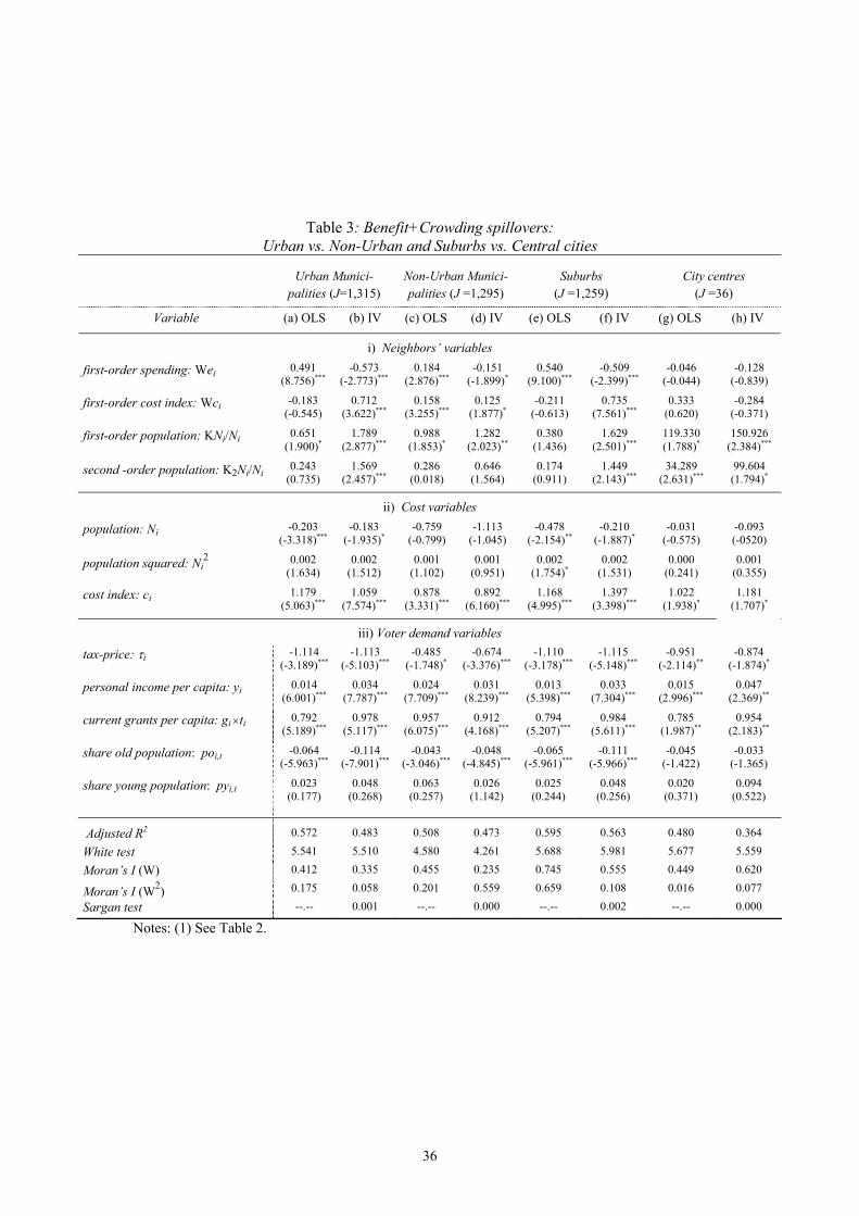
36

Table 3: Benefit+Crowding spillovers: Urban vs. Non-Urban and Suburbs vs. Central cities

Urban Munici- palities (J=1,315)

Non-Urban Munici-palities (J =1,295)

Suburbs (J =1,259)

City centres (J =36)

Variable (a) OLS (b) IV (c) OLS (d) IV (e) OLS (f) IV (g) OLS (h) IV

i) Neighbors’ variables

first-order spending: Wei 0.491 (8.756)***

-0.573 (-2.773)***

0.184 (2.876)***

-0.151 (-1.899)*

0.540 (9.100)***

-0.509 (-2.399)***

-0.046 (-0.044)

-0.128 (-0.839)

first-order cost index: Wci -0.183 (-0.545)

0.712 (3.622)***

0.158 (3.255)***

0.125 (1.877)*

-0.211 (-0.613)

0.735 (7.561)***

0.333 (0.620)

-0.284 (-0.371)

first-order population: KNi/Ni 0.651 (1.900)*

1.789 (2.877)***

0.988 (1.853)*

1.282 (2.023)**

0.380 (1.436)

1.629 (2.501)***

119.330 (1.788)*

150.926 (2.384)***

second -order population: K2Ni/Ni 0.243 (0.735)

1.569 (2.457)***

0.286 (0.018)

0.646 (1.564)

0.174 (0.911)

1.449 (2.143)***

34.289 (2.631)***

99.604 (1.794)*

ii) Cost variables

population: Ni -0.203 (-3.318)***

-0.183 (-1.935)*

-0.759 (-0.799)

-1.113 (-1.045)

-0.478 (-2.154)**

-0.210 (-1.887)*

-0.031 (-0.575)

-0.093 (-0520)

population squared: Ni2 0.002

(1.634) 0.002

(1.512) 0.001

(1.102) 0.001

(0.951) 0.002

(1.754)* 0.002

(1.531) 0.000

(0.241) 0.001

(0.355)

cost index: ci 1.179 (5.063)***

1.059 (7.574)***

0.878 (3.331)***

0.892 (6.160)***

1.168 (4.995)***

1.397 (3.398)***

1.022 (1.938)*

1.181 (1.707)*

iii) Voter demand variables tax-price: τi -1.114

(-3.189)*** -1.113

(-5.103)***-0.485

(-1.748)* -0.674

(-3.376)***-1.110

(-3.178)*** -1.115

(-5.148)*** -0.951

(-2.114)** -0.874

(-1.874)*

personal income per capita: yi 0.014 (6.001)***

0.034 (7.787)***

0.024 (7.709)***

0.031 (8.239)***

0.013 (5.398)***

0.033 (7.304)***

0.015 (2.996)***

0.047 (2.369)**

current grants per capita: gi ×ti 0.792 (5.189)***

0.978 (5.117)***

0.957 (6.075)***

0.912 (4.168)***

0.794 (5.207)***

0.984 (5.611)***

0.785 (1.987)**

0.954 (2.183)**

share old population: poi,t -0.064 (-5.963)***

-0.114 (-7.901)***

-0.043 (-3.046)***

-0.048 (-4.845)***

-0.065 (-5.961)***

-0.111 (-5.966)***

-0.045 (-1.422)

-0.033 (-1.365)

share young population: pyi,t 0.023 (0.177)

0.048 (0.268)

0.063 (0.257)

0.026 (1.142)

0.025 (0.244)

0.048 (0.256)

0.020 (0.371)

0.094 (0.522)

Adjusted R2 0.572 0.483 0.508 0.473 0.595 0.563 0.480 0.364

White test 5.541 5.510 4.580 4.261 5.688 5.981 5.677 5.559

Moran’s I (W) 0.412 0.335 0.455 0.235 0.745 0.555 0.449 0.620

Moran’s I (W2) 0.175 0.058 0.201 0.559 0.659 0.108 0.016 0.077

Sargan test --.-- 0.001 --.-- 0.000 --.-- 0.002 --.-- 0.000

Notes: (1) See Table 2.

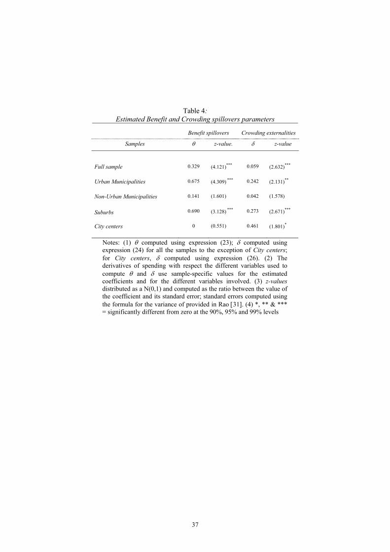
37

Table 4: Estimated Benefit and Crowding spillovers parameters

Benefit spillovers Crowding externalities

Samples θ z-value. δ z-value

Full sample 0.329 (4.121)*** 0.059 (2.632)***

Urban Municipalities 0.675 (4.309) *** 0.242 (2.131)**

Non-Urban Municipalities 0.141 (1.601) 0.042 (1.578)

Suburbs

0.690 (3.128) *** 0.273 (2.671)***

City centers 0 (0.551) 0.461 (1.801)*

Notes: (1) θ computed using expression (23); δ computed using expression (24) for all the samples to the exception of City centers; for City centers, δ computed using expression (26). (2) The derivatives of spending with respect the different variables used to compute θ and δ use sample-specific values for the estimated coefficients and for the different variables involved. (3) z-values distributed as a N(0,1) and computed as the ratio between the value of the coefficient and its standard error; standard errors computed using the formula for the variance of provided in Rao [31]. (4) *, ** & *** = significantly different from zero at the 90%, 95% and 99% levels

SÈRIE DE DOCUMENTS DE TREBALL DE L'IEB

2000 2000/1 - Esteller, A.; Solé, A., "Vertical Income Tax Externalities and Fiscal Interdependence: Evidence from the US" Publicat a: Regional Science and Urban Economics, 31 (2-3), pàgs. 247-72, 2001. 2000/2 - Castells, A., "The role of intergovernmental finance in achieving diversity and cohesion: the case of Spain" Publicat a: Environment and Planning C: Government and Policy, 19 (2), pàgs. 189-206, 2001. 2000/3 - Costa, M.T.; Segarra, A. (URV); Viladecans, E., "Pautas de localización de las nuevas empresas y flexibilidad territorial" Publicat a: Small Business Economics, 22(3-4), pàgs. 265-281, 2004, sota el títol "The location of new firms and the lifecycle of industries". 2000/4 - Costa, M.T.; Duch, N.; Lladós, J. (UAB), "Determinantes de la innovación y efectos sobre la competitividad: el caso de las empresas textiles" Publicat a: Revista Asturiana de Economía, 20, pàgs. 53-80, 2001. 2000/5 - Solé, A., "Determinantes del gasto público local: necesidades de gasto vs. capacidad fiscal" Publicat a: Revista de Economía Aplicada, 9 (25), pàgs. 115-56, 2001, sota el títol "Determinantes del gasto público local: ¿Necesidades de gasto o capacidad fiscal?" 2000/6 - Barberán, R. (U. de Zaragoza); Bosch, N.; Castells, A.; Espasa, M., "The redistributive power of the Central Government Budget"

2001 2001/1 - Espasa, M., "The territorial redistribution of the EU budget. Empirical evidence at national and regional level" Publicat a: Enviroment and Planning C: Government and Policy, 19 (5), pàgs. 771-790, 2001, sota el títol "The territorial redistributive power of the EU budget. Empirical evidence at national and regional level" 2001/2 - Viladecans, E., "La concentración territorial de las empresas industriales: un estudio sobre la unidad geográfica de análisis mediante técnicas de econometría espacial" Publicat a: Papeles de Economía Española, 89/90, pàgs. 308-320, 2001, sota el títol "La concentración territorial de las empresas industriales. Un estudio sobre el tamaño de las empresas y su proximidad geográfica" 2001/3 - Castells, A., "La descentralización de las políticas sociales en el Estado del Bienestar" 2001/4 - Bosch, N.; Pedraja, F. (U. de Extremadura); Suárez-Pandiello, J. (U. de Oviedo), "The influence of Environmental Variables in Measuring the Efficiency of Refuse Collection Services: An Application to the Spanish Municipalities" Publicat a: Local Government Studies, 26 (3), pàgs. 71-90, 2000. 2001/5 - Solé, A., "Budget spillovers in a metropolitan area: typology and empirical evidence" 2001/6 - Sanromà, E.; Ramos, R. (UB-AQR), "Local human capital and external economies: evidence for Spain" 2001/7 - Leonida, L. (U. Della Calabria); Montolio, D., "Convergence and Inter-Distributional Dynamics among the Spanish Provinces. A Non-parametric Density Estimation Approach"

SÈRIE DE DOCUMENTS DE TREBALL DE L'IEB

2001/8 - García Quevedo, J., "University research and the location of patents in Spain" Publicat a: Papeles de Economía Española, 93 pàgs. 98-108, sota el títol "Investigación universitaria y localización de las patentes en España" 2001/9 - Esteller, A.; Solé A., "Tax Setting in a Federal System: The Case of Personal Income Taxation in Canada" Publicat a: International Tax and Public Finance, 9, pàgs. 235-57, 2002, sota el títol "An empirical analysis of vertical tax externalities: The case of personal income taxation in Canada" 2001/10 - Durán J.M.; Gispert, C. de, "Fiscalidad medioambiental sobre la energía: propuestas para España " Publicat a: Energía, fiscalidad y medio ambiente en España, a A. Gago i X. Labandeira (Dir.), 7, pàgs. 171-192, 2002, sota el títol "La imposición energético-ambiental en España" 2001/11 - Álvarez, M., "España y la senda de desarrollo de la inversión directa: una aproximación"

2002 2002/1 - Bosch, N.; Espasa, M.; Sorribas, P., "La capacidad redistributiva y estabilizadora del presupuesto del Gobierno Central Español" Publicat a: Hacienda Pública Española/Revista de Economía Pública, 160 (1), pàgs. 47-76, 2002. 2002/2 - García Quevedo, J., "The location of innovation. Universities and technological infrastructure in Spain" 2002/3 - Viladecans Marsal, E., "The growth of cities: Does agglomeration matter?" 2002/4 - Pons Novell, J.; Tirado Fabregat, D.A. (UB), "Discontinuidades en el crecimiento económico en el periodo 1870-1994: España en perspectiva comparada" 2002/5 - Bosch, N.; Espasa, M.; Sorribas, P., "The redistributive, stabiliser and insurance effects at territorial level of "federal" government budgets" 2002/6 - Callejón, M. (UB); García Quevedo, J., "Las ayudas públicas a la I+D empresarial. Un análisis sectorial"

2003 2003/1 - Solé Ollé, A.; Viladecans Marsal, E., "Fiscal and growth spillovers in large urban areas" 2003/2 - Gual, J. (IESE); Trillas, F., "Telecommunications Policies: Determinants and Impact" 2003/3 – Leonida, L. (U. Della Calabria); Montolio, D., “Public Capital, Growth and Convergence in Spain. A Counterfactual Density Estimation Approach” 2003/4 – Álvarez, M., “FDI Determinant Factors: The Case of Catalan Multinational Manufacturing Firms” 2003/5 – Álvarez, M., “Wholly-Owned Subsidiaries Versus Joint Venture: The Determinant Factors in the Catalan Multinational Manufacturing Case” 2003/6 – Pelegrín, A., “Regional Distribution of Foreign Manufacturing Investment in Spain. Do agglomeration economies matter?”

SÈRIE DE DOCUMENTS DE TREBALL DE L'IEB

2004 2004/1 – Sánchez Hugalde, A., "Movilidad intergeneracional de ingresos y educativa en España (1980-90)" 2004/2 – Esteller, A., "Tax Evasion in Interrelated Taxes" 2004/3 – Castells, A.; Esteller, A.; Vilalta, M., "Full Characterisation of the Political Economy of Fiscal Adjustment: Evidence from Spanish Municipalities" 2004/4 – Lambert, P.J. (U. of York), "Income Taxation and Equity" 2004/5 – Bosch, N.; Solé, A., "Yardstick competition and the political costs of raising taxes: An empirical analysis of Spanish municipalities" 2004/6 – Maggioni, M. (U. Cattolica del Sacro Cuore), "The rise and fall of industrial clusters: Technology and the life cycle of regions" 2004/7 – Frey, B.S. (U. of Zurich); Torgler, B. (U. of Basel), "Taxation and Conditional Cooperation" 2004/8 – Alonso, J.; Freire-Serén, M.J.; Manzano, B., "Rentabilidad social de la inversión pública española en infraestructruras"

2005 2005/1 - Arocena, P.; "The measurement of scope, scale and diversification economies: How (in)efficient is electricity restructuring and unbundling?" 2005/2 – Solé Ollé, A.; " The effects of party competition on budget outcomes: Empirical evidence from local governments in Spain "