Barcelona GSE Working Paper Series

Working Paper nº 944

Expectations, Satisfaction, and Utility from Experience Goods: A Field

Experiment in Theaters

Ayelet Gneezy Uri Gneezy Joan Llull

Pedro Rey-Biel

Expectations, Satisfaction, and Utility from Experience Goods: A Field

Experiment in Theaters∗

Pedro Rey-Biel∗∗, Ayelet Gneezy, Uri Gneezy and Joan Llull

November 30, 2016

Abstract

Understanding what affects satisfaction from consumption is fundamental

to studying economic behavior. However, measuring subjective hedonic

experiences is not trivial, in particular when studying experience goods in

which quality is difficult to observe prior to consumption. We report the

results of a field experiment with a theater show in which the audience

pays at the end of the show under pay-what-you-want pricing. Using

questionnaires, we measure expected enjoyment before the show, as well

as the realized enjoyment after. Correlating the amounts paid with the

expected and realized enjoyment, we find that individuals with a larger

gap between reported expectations and enjoyment pay significantly more.

Once we account for the satisfaction gap, the level of expected enjoyment

or realized enjoyment has no significant effect in predicting payments.

Keywords: experience goods; pay-what-you-want; expectations.

JEL classification: C72; C91; D81.

∗We are grateful to Sala Beckett and Sixto Paz Producciones for their collaboration on this project. We thank Miguel A. Ballester, Marco Bertini, Guillaume Hollard, Steffen Huck, Alex Imas, Wieland Müller, Marta Serra-García, Sigrid Suetens, Matthias Sutter and seminar participants at several institutions for their comments, and Adrià Bronchal, Elena Costas-Pérez, Sergi Martínez, Dilan Okçuoğlu, and Javier Rodríguez-Camacho for excellent research assistance. We acknowledge financial support from Programa Ramón y Cajal, Ministerio de Economía y Competitividad (ECO2012-31962, ECO2014-59056-JIN, ECO2015-63679-P and through the Severo Ochoa Programme for Centres of Excellence in R&D (SEV-2011-0075 and SEV-2015-0563)), Fundación Areces and Barcelona GSE. ∗∗Corresponding author: Universitat Autònoma de Barcelona and Barcelona Graduate School of Economics. Department d’Economia i d’Historia Econòmica, 08193 Bellaterra. Barcelona (Spain). Tel: (+34) 935812113. E-mail: pedro.rey@uab.es.

2

1. Introduction

Understanding what affects satisfaction from consumption is fundamental to

studying economic behavior. However, measuring subjective hedonic experiences is not

trivial, in particular when studying experience goods in which quality is difficult to

observe prior to consumption.1

Recent literature suggested that expectations may have an important impact on

satisfaction (Koszegi and Rabin, 2006; Schwartz, 2005). Traditional measures of post-

consumption utility, using subjective evaluation based on questionnaires, cannot inform

us about how expectations and satisfaction interact. Hence, clever experimental designs

have been used to show indirect evidence of a reference-dependent component in utility

functions, based on how the intrinsic value of an outcome compares to expectations

(Kahneman and Tversky, 1979; Medvec, Madey and Gilovich, 1995; Card and Dahl,

2008; Abeler et al., 2012; Bushong and Gagnon-Bartsch, 2016). However, finding direct

empirical evidence regarding how expectations and utility interact has proven elusive due

to three main reasons. First, people need to actually consume the good or experience,

preferably in a naturally occurring environment. Second, the researcher needs individual-

level data to measure each participant’s expectations prior to consumption, as well as

satisfaction post-consumption. Finally, capturing the utility associated with the

consumption of an experience good is far from trivial.2

We address these difficulties using a unique dataset obtained in a field experiment

conducted in theaters in which participants were the regular audience, and hence were

actually consuming a good of their choice in a natural environment over time. To address

1 See Nelson (1970). In some cases, quality is hard to measure even post consumption, as in the case of credence goods (Darbi and Karni, 1973; Dullek et al, 2011 and Balafoutas et al, 2013). 2 Kahneman, Wakker, and Sarin (1997) distinguish between two types of utility: “decision utility,” in which utility is inferred from observed choices and is used to describe ordinal ranking, and “experienced utility,” based on pleasure and pain. Our discussion relates to the second type in which measuring the subjective hedonic experience is harder because it is not observed.

3

the individual-level data concern, all participants took a short survey before and after the

show. Finally, we measured consumption utility using a “pay-what-you-want” (PWYW)

pricing scheme at the end of the show, in which participants chose how much, including

zero, they wished to pay for the show (Gneezy et al., 2010) and we were able to link

payment data to questionnaire measures at the individual level.3

Importantly, we show that subjective post-consumption evaluations capture only

part of the picture. The difference between expectations and post-consumption

evaluations is also important. People form expectations regarding the quality of future

consumption, and the difference between these expectations and actual experience

derives the overall satisfaction of that experience. In contrast with the literature discussed

above, it is not simply true that lower expectations result in higher payment. Among

individuals stating the same expectations or enjoyment, those with a greater gap between

expected and actual enjoyment pay significantly more. Once the satisfaction gap is

accounted for, neither the level of expectation nor enjoyment predict payments. These

findings are important both for the measuring and understanding of utility from

experience goods as well as having important implications with respect to the way

experience goods should be marketed and priced. In particular, the importance of

expectations sets an interesting trade-off when marketing an experience good between

appealing to a larger set of consumers and disappointing them. Similarly, using pay-what-

you-want pricing allows to resolve consumers’ uncertainty linked to the unknown quality

of the experience good while, which may positively affect revenue with respect to

traditional pricing.

3 This approach is similar to what has been studied in the tipping literature, although we use a much richer data set, which allows us to also measure expectations and satisfaction and relate payment to the experience itself, separated from potential confounds such as exceptional service provided. See Lynn (2006) and Azar (2007) for reviews.

4

2. Setting and Procedure

We ran the study over 19 (out of 40) performances of a fully booked play, “The

Effect” by Lucy Prebble, at Sala Beckett in Barcelona (January-March 2015). The 19

performances in the sample are from the later part of the 40, since the earlier shows were

used to fine-tune our intervention. The producers of this show, Sixto Paz Produccions,4

have been using PWYW pricing for all their spectacles since 2011. In their regular

operating procedure, the audience pre-book tickets at no cost, knowing that upon exit

from the theater, they will be asked to pay whichever amount they see fit, including zero.

In our study, we maintained the same PWYW procedures.5

On each of the evenings of the experiment, we asked approximately one third of

the espectators to complete short questionnaires, one prior to and the other after the show,

measuring expectations, enjoyment, and demographic variables.

To allow for randomization, a member of our research team approached

individuals based on constant time intervals upon arrival to the theatre. Participants were

asked whether they were willing to take part in a study. This question seemed natural to

the audience because the topic of the play dealt with medical trials, and our

questionnaires, resembling clinical trial consent forms, were a participatory activity

enhancing the theatre experience. Sixto Paz Productions regularly integrates

questionnaires, games, and small focus groups, both before and after their plays in their

shows. Participants were also asked to randomly pick one of two differently colored pills

from a bowl, and were told the pill could either be a placebo or one “helping us to study

4 https://www.facebook.com/SixtoPazProduccions/ 5 PWYW and other similar pricing schemes are increasingly being adopted in theaters. We are aware of

companies using such schemes in cities such as Amsterdam, Edinburgh, London, Los Angeles, Madrid and

Philadelphia.

5

whether it made them enjoy the play more.” We do not find a statistically significant

effect of taking the pill on the distribution of answers to any variable in the questionnaires

nor on payments. Figure A1 in the Appendix shows a completed example of both

questionnaires (in Catalan) and a translation of the questions into English.

Participants were told the show was being video recorded, and that for legal

reasons, we needed their signed consent agreeing to be seated in a theatre area where the

camera could capture their image. From the participants we approached, 629 (92%)

agreed to take part in all activities. Upon agreement, participants were given the pre-

performance questionnaire, which also automatically assigned them a seat. The

questionnaire captured basic demographic questions (age, gender, and occupation),

theater-attendance habits, who booked the tickets (self or someone else), and how many

people were included in the reservation. Most crucially, participants indicated the extent

to which they expected to enjoy the play on a 7-point scale.

At the end of the play, participants placed the pre-performance questionnaires,

together with their payment, in one of two boxes located on a table where the show’s

producer was standing. The only difference in payment procedure between the study

participants and the other audience members was that participants placed their payment

on top of their questionnaire, allowing us to trace their seat numbers.

Once participants exited the stage hall, they received a second questionnaire

asking them to rate their enjoyment using a 7-point scale (questionnaires were associated

with visitors’ seat number). The questionnaire also included 4-point-scale questions on

the likelihood of recommending the show to others and on whether expectations were

met, a 7-point-scale question on agreement with the message of the play and the

6

possibility of writing additional comments. After completing this second questionnaire,

participants left the theater.

The hypotheses we can test with our data are simple. First, high expectations

might lower the overall enjoyment; hence,

Hypothesis 1 (H1): Payments decrease with expected enjoyment.

Second, actual reported enjoyment may affect payment:

Hypothesis 2 (H2): Payments increase with realized enjoyment.

Finally, the gap (realized enjoyment minus expected enjoyment) might predict payment:

Hypothesis 3 (H3): Payments increase with the enjoyment gap.

3. Results

Comparing participants, non-participants, and regular audience

Before analyzing the experimental data, we test whether taking part in our study affected

payments. We how much participants whose payment we can individually trace back

(N=539) with the payments of the remaining audience members during the 19 nights in

which we conducted our experiment (N=1,221; labeled “non-participants”) and with the

payments of all audience members in the remaining 21 nights (N=1,658; labeled “regular

audience”). All 40 nights were charged using PWYW. Figure 1 shows the probability

density and cumulative distribution functions of payments of all three groups. As can be

seen, the distribution of payments for the three groups is practically identical, implying

our intervention did not influence payments. Kolmogorov-Smirnov tests of the hypothesis

7

that each pair-wise comparison of the two empirical distributions comes from the same

population distribution do not reject the null hypothesis in any case.

FIGURE 1. DISTRIBUTION OF PAYMENTS (PARTICIPANTS, NON-PARTICIPANTS, AND REGULAR AUDIENCE)

Note.- The figure plots the distribution of payments for “participants” (blue), “non-participants” during experiment

days (light blue), and “regular audience” members (during non-experiment days; dark blue). The left figure shows

kernel density estimates, whereas the right figure depicts the empirical cummulative distribution functions for the three

samples. A Kolmogorov-Smirnov test of the hypothesis that the two empirical distributions come from the same

population distribution cannot reject the null hypothesis. P-values are 0.6, 0.42, and 0.75 for the comparison of

participants and non-participants, participants and regular audience, and non-participants and regular audience,

respectively.

We also distributed additional questionnaires to non-participants in the last four nights of

the run, producing additional samples of 148 answers to the first questionnaire and 197

answers to the second one. These questionnaires are not linked individually and do not

have associated payment information. Figures A2 through A4 (see Appendix) show that

neither the expectations, enjoyment, or other reported characteristics differ between

participants and respondents to these additional questionnaires (to which we refer as

“other audience”), with two exceptions: experiment participants were somewhat older

(4.4 years on average, with a standard error of 0.84) and also attended the show in larger

groups (0.43 additional group members, with a standard error of 0.14). We control for

these variables in all analyses.

8

TABLE 1. DESCRIPTIVE STATISTICS

Average Std. Dev. Min Max

Age 37.45 13.03 16 88

Female 0.64 0.48 0 1

Paid in group 0.62 0.49 0 1

Number of accomp. Persons 2.39 1.48 0 5

First time at venue 0.46 0.50 0 1

Times at venue before 2.15 3.11 0 10

First time theatre in a year 0.09 0.28 0 1

Times in theatre last year 8.11 12.68 0 90

Note.- The table lists averages, standard deviations, and extremum values for a set of demographic characteristics and

theater-attendance habbits of participants.

Descriptive statistics

Table 1 presents the descriptive statistics of demographic variables and theater-

attendance habits. Participants’ age ranges from 16 to 88 years old, with an average age

of 37 years, and 64% were females. Approximately half the participants (54%) had

attended shows at the specific venue, where shows by other companies using traditional

pricing systems are also run. Most participants (91%) attended several theater shows

during the preceding year (8 shows on average). Of all participants, 62% paid in groups,

in which case we assign an equal fraction of payment to each group member.

Independently of whether participants paid in groups, the average number of

accompanying persons was 2.39.

Table 2 shows descriptive statistics of expectations, enjoyment data, and

payments. Payments range from 2.50 to 35 euros, with an average payment of 12.86

euros, which is above the typical price of 10 euros for independent theater plays in

Barcelona.6

6 Participants who did not pay any amount are indistinguishable from those who did not return the ex-ante

questionnaire and whose payment may be accounted as nonparticipants’ payment (which we cannot trace

individually). Taking this into account, the proportion of participants for which we do not have payment

9

TABLE 2.DESCRIPTIVE STATISTICS OF PAYMENT, EXPECTATIONS, AND ENJOYMENT MEASURES

Average Std. Dev. Min Max

Payment 12.86 4.96 2.50 35.00

Reported enjoyment measures:

Expected enjoyment 6.20 0.81 3 7

Realized enjoyment 5.92 0.99 2 7

Other reported measures:

Expectations were met 3.04 0.59 1 4

Likelihood of recommend. 3.55 0.68 0 4

Agreement with message 5.73 1.09 0 7

Note.- The table includes means, standard deviations, and the range of values (min and max) for the different variables

used in the analysis. Except for “other reported measures,” statistics are computed for the subsample of 433 participants

for which information for all these variables is available. The subsamples used to compute each of the three last rows

include, respectively, 433, 434, and 419 observations.

Reported measures of both expected and realized enjoyment show that, in general,

attendants expected a high-quality show and enjoyed the experience. On a scale from 1 to

7, the average expected enjoyment is 6.20, which is slightly above the average declared

realized enjoyment (5.92). Expected enjoyment does not significantly correlate with

descriptive variables in Table 1, with the exception of gender and whether participants

were visiting the venue for the first time.7 Participants booking tickets themselves do not

show significant higher average expectations than does who do not.

In reply to the 4-point-scale question about whether the show met audience

expectations, the average reported level was 3.04. Regarding the likelihood of

recommending the show to others, the average answer was 3.55, also on a 4-point scale.

data is relatively low (14.15%) and higher compared with the proportion of non-participants (which may

include participants) who did not pay (8.4%). 7 Female participants have on average significantly higher expected enjoyment, and also realized

enjoyment. In turn, gender is not significantly correlated with the difference between realized and expected

enjoyment, which we later define as the “gap”.

10

Finally, the degree of agreement with the play’s message was 5.73 on a 7-point scale.8

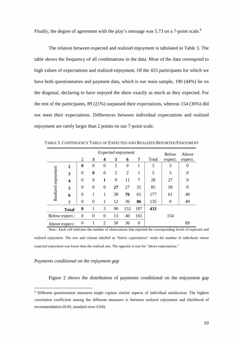
The relation between expected and realized enjoyment is tabulated in Table 3. The

table shows the frequency of all combinations in the data. Most of the data correspond to

high values of expectations and realized enjoyment. Of the 433 participants for which we

have both questionnaires and payment data, which is our main sample, 190 (44%) lie on

the diagonal, declaring to have enjoyed the show exactly as much as they expected. For

the rest of the participants, 89 (21%) surpassed their expectations, whereas 154 (36%) did

not meet their expectations. Differences between individual expectations and realized

enjoyment are rarely larger than 2 points on our 7-point scale.

TABLE 3. CONTINGENCY TABLE OF EXPECTED AND REALIZED REPORTED ENJOYMENT

Expected enjoyment Below expect.

Above expect. 2 3 4 5 6 7 Total

Rea

lized

enj

oym

ent

2 0 0 0 2 0 1 3 3 0

3 0 0 0 2 2 1 5 5 0

4 0 0 1 9 11 7 28 27 0

5 0 0 0 27 27 31 85 58 0

6 0 1 1 38 76 61 177 61 40

7 0 0 1 12 36 86 135 0 49

Total 0 1 3 90 152 187 433

Below expect.: 0 0 0 13 40 101 154

Above expect.: 0 1 2 50 36 0 89

Note.- Each cell indicates the number of observations that reported the corresponding levels of expected and

realized enjoyment. The row and column labelled as “below expectations” totals the number of indivduals whose

expected enjoyment was lower than the realized one. The opposite is true for “above expectations.”

Payments conditional on the enjoyment gap

Figure 2 shows the distribution of payments conditional on the enjoyment gap

8 Different questionnaire measures might capture similar aspects of individual satisfaction. The highest

correlation coefficient among the different measures is between realized enjoyment and likelihood of

recommendation (0.69, standard error 0.04).

FIGURE 2. DISTRIBUTION OF PAYMENTS CONDITIONAL ON ENJOYMENT GAP

Note.- The figure shows the distribution of payments conditional on the enjoyment gap. The position of a bubble

indicates a pair of amount paid and enjoyment gap. The size of the bubble indicates the number of individuals that are

in a given pair. The black line plots the average payment conditional on the enjoyment gap.

(realized enjoyment minus expected enjoyment). Importantly, the figure shows the

conditional mean of payments has an upward trend. That is, mean payments increase as

the enjoyment gap increases.

Figure 3 confirms (based on regression results reported below) that payments

increase with the enjoyment gap. The four panels depict the average payment (in levels in

the upper panels, in logarithms in the lower panels) as the enjoyment gap increases

conditional on the different levels of expected enjoyment (left panels) or realized

enjoyment (right panels). The black solid lines depict the fitted values of a quadratic

regression of payment (or log payment) on the enjoyment gap, showing again a clear

increasing trend. The 95% confidence intervals, shown in dotted lines, confirm the

increasing trend. The fact that each of the increasing colored lines basically lie on top of

FIGURE 3. AVERAGE PAYMENT (LEVEL AND LOG) BY ENJOYMENT GAP AND LEVEL

Note.- Colored solid lines in each plot represent the average payment (top plots) or log payment (bottom plots) for each

gap level for the subsamples of individuals with the indicated expected or realized enjoyment. Only the averages of

cells with more than five observations are reported. Black solid lines depict the fitted values of a regression of payment

(or log payment) on a second-order polynomial on the enjoyment gap. Dotted lines indicate 95% confidence intervals.

each other indicates the difference between expected and realized enjoyment is really the

important determinant of payment, over and above the reported level of enjoyment. This

is the main result of our paper, which we confirm using controls in the regression analysis

presented in the next section.

Regression Results

We run a regression of log payment on different measures of enjoyment and the

controls summarized in Table 1. Table 4 shows the main results from this regression.

TABLE 4. REGRESSION RESULTS: LOG PAYMENT ON ENJOYMENT LEVELS AND GAPS

(1) (2) (3) (4) (5) (6)

Constant 2.407 1.834 2.125 2.240 1.946 2.116

(0.177) (0.139) (0.188) (0.075) (0.214) (0.106)

Enjoyment gap --- --- --- 0.071 --- 0.069

(0.018) (0.018)

Expected enjoyment -0.035 --- -0.059 --- -0.051 ---

(0.025) (0.025) (0.027)

Realized enjoyment --- 0.067 0.078 --- 0.079 ---

(0.020) (0.020) (0.020)

Age 0.010 0.010 0.010 0.010 0.010 0.010

(0.002) (0.002) (0.002) (0.002) (0.002) (0.002)

Female 0.012 -0.024 -0.009 -0.002 -0.013 -0.003

(0.032) (0.032) (0.033) (0.030) (0.034) (0.031)

Paid in group -0.063 -0.075 -0.069 -0.067 -0.053 -0.050

(0.041) (0.040) (0.040) (0.040) (0.040) (0.040)

Num. of accomp. pers. (base=1):

0 0.069 0.043 0.046 0.049 0.080 0.083

(0.167) (0.160) (0.167) (0.169) (0.168) (0.170)

2 -0.102 -0.087 -0.101 -0.105 -0.091 -0.097

(0.078) (0.077) (0.074) (0.074) (0.077) (0.076)

3 -0.061 -0.049 -0.053 -0.055 -0.027 -0.031

(0.056) (0.055) (0.054) (0.055) (0.060) (0.060)

4 -0.081 -0.085 -0.090 -0.090 -0.086 -0.088

(0.055) (0.056) (0.056) (0.056) (0.057) (0.057)

5 or more -0.069 -0.057 -0.060 -0.062 -0.067 -0.070

(0.065) (0.061) (0.061) (0.062) (0.067) (0.068)

First time at venue -0.038 -0.043 -0.056 -0.057 -0.024 -0.026

(0.040) (0.040) (0.039) (0.039) (0.041) (0.040)

First time at theatre this year -0.057 -0.080 -0.083 -0.081 -0.108 -0.103

(0.073) (0.071) (0.070) (0.071) (0.069) (0.071)

Night fixed effects No No No No Yes Yes

Expected+Realized = zero (p-val) --- --- 0.479 --- 0.319 ---

Restricted vs unrestricted (p-val) --- --- --- 0.497 --- 0.315

Adjusted R-squared 0.125 0.149 0.162 0.162 0.188 0.187

Num. of observations 433 433 433 433 433 433

Note.- The table includes regression coefficients for a set of regressions of log payment on a set of controls, reported

enjoyment (expected and/or realized), and/or the enjoyment gap, as indicated. Night fixed effects are included in

columns 5 and 6 as indicated. Reported p-values correspond to tests of the null hypothesis that the coefficients of

expected and realized enjoyment are equal in absolute value and of opposite sign and to a test comparing the restrictred

and unrestricted models. Standard errors clustered by joint-payment groups are reported in parentheses.

14

Columns (1)–(4) do not include night fixed effects, whereas columns (5) and (6) do. Among

the controls, the age coefficient is always positive and significant, indicating older people

pay more, which makes sense because age is a good proxy for income.9 Column (1) shows

expected enjoyment by itself is not a significant determinant of payment, whereas column

(2) shows realized enjoyment is. When including both regressors in column (3), the fit

improves (the adjusted R2 increases from 0.149 to 0.162) and both coefficients become

significant. We cannot reject the null hypothesis that the magnitude of both coefficients is

the same. Interestingly, the two coefficients are similar in magnitude and of opposite sign

(p-value=0.479), which means that in terms of payment, the effect of lowering expectations

by one unit is the same as the effect of increasing realized enjoyment by one unit, and the

difference between the two is what matters. This is in line with the results in Figure 3, where

the payment curves by expected and realized enjoyment levels lie on top of each other. The

result is confirmed in column (4) where the coefficient of the enjoyment gap is signicant and

positive, showing a 7% increase in payment (1 euro for the average individual) for each

extra unit in the enjoyment gap. We cannot reject the hypothesis that the restricted and

unrestricted models are identical (p-value=0.497). Including fixed effects in columns (5) and

(6) increases the R2, and the coefficients are virtually unchanged. This confirms the

enjoyment gap is a sufficient statistic of expected and realized enjoyment in the payment

function.

As is apparent from Figure 3, the relation between the enjoyment gap and

payment is likely non-linear. Table 5 studies the nature of this relationship introducing

quadratic and cubic polynomials in the enjoyment gap and the coefficients on the levels

in the regressions. Estimated coefficients show evidence in favor of a quadratic

9 Table A1 in the Appendix, shows average payment and satisfaction measures for selected groups created

according to each of the questions in the ex-ante questionnaire. Older audience members pay more, regular

theater attendants pay more, and those paying in groups pay less.

TABLE 5. REGRESSION RESULTS: NON-LINEAR RELATION BETWEEN LOG PAYMENT AND

ENJOYMENT GAP

(1) (2) (3) (4) (5) (6)

Enjoyment gap 0.059 0.051 0.050 0.046 0.042 0.036

(0.025) (0.027) (0.027) (0.028) (0.028) (0.030)

Enjoyment gap squared --- --- -0.016 -0.017 -0.011 -0.010

(0.008) (0.008) (0.012) (0.011)

Enjoyment gap cubed --- --- --- --- 0.002 0.002

(0.003) (0.003)

Realized enjoyment 0.020 0.029 0.005 0.013 0.007 0.018

(0.028) (0.029) (0.028) (0.029) (0.028) (0.029)

Controls Yes Yes Yes Yes Yes Yes

Night fixed effects No Yes No Yes No Yes

Slope for gap is zero (p-val) 0.022 0.059 0.002 0.007 0.002 0.020

Level coeff. is zero (p-val) 0.479 0.319 0.846 0.656 0.799 0.545

Adjusted R-squared 0.162 0.188 0.166 0.095 0.165 0.190

Num. of observations 433 433 433 433 433 433

Note.- The table includes gap polynomials and level coefficients from regressions of log payment on these variables, a

set of controls, and, whenever indicated, night fixed effects. Included controls coincide with those in Table 4. Reported

p-values correspond to tests of joint significance of the gap polynomial coefficients, and of individual significance of

the coefficient of realized enjoyment. Standard errors, clustered by joint-payment groups, are reported in parentheses.

relationship but not a cubic one. A test of joint significance of the gap polynomial

coefficients rejects that the slope is zero at the 95% level.10 We cannot reject that the

estimated level coefficients of realized enjoyment are zero, confirming that, conditional

on expected enjoyment, estimated payment is the same for the same enjoyment gap.

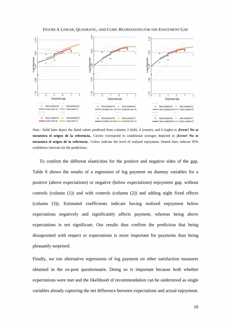
Linking these results back to Figure 3, Figure 4 depicts the fitted values predicted

from columns (2) (left), (4) (center), and (6) (right) in Table 5. Circles correspond to the

conditional averages plotted in Figure 3. Different colors indicate the conditioning levels

of realized enjoyment. The results show the quadratic and cubic specifications deliver

almost identical predictions, and that they fit the conditional averages much better than

the linear model. More specifically, they show a steeper slope for negative values of the

gap, but a rather flat shape for positive values.

10 At the 90% level for the linear model including night fixed effects.

16

FIGURE 4. LINEAR, QUADRATIC, AND CUBIC REGRESSIONS FOR THE ENJOYMENT GAP

Note.- Solid lines depict the fitted values predicted from columns 2 (left), 4 (center), and 6 (right) in ¡Error! No se

encuentra el origen de la referencia.. Circles correspond to conditional averages depicted in ¡Error! No se

encuentra el origen de la referencia.. Colors indicate the level of realized enjoyment. Dotted lines indicate 95%

confidence intervals for the predictions.

To confirm the different elasticities for the positive and negative sides of the gap,

Table 6 shows the results of a regression of log payment on dummy variables for a

positive (above expectations) or negative (below expectations) enjoyment gap, without

controls (column (1)) and with controls (column (2)) and adding night fixed effects

(column (3)). Estimated coefficients indicate having realized enjoyment below

expectations negatively and significantly affects payment, whereas being above

expectations is not significant. Our results thus confirm the prediction that being

dissapointed with respect to expectations is more important for payments than being

pleasantly surprised.

Finally, we run alternative regressions of log payment on other satisfaction measures

obtained in the ex-post questionnaire. Doing so is important because both whether

expectations were met and the likelihood of recommendation can be understood as single

variables already capturing the net difference between expectations and actual enjoyment.

TABLE 6. REGRESSIONS FOR ENJOYMENT BELOW, AT PAR, AND ABOVE EXPECTATIONS

(1) (2) (3)

Above expectations 0.000 0.022 0.013

(0.049) (0.049) (0.048)

Below expectations -0.111 -0.124 -0.125

(0.044) (0.039) (0.039)

Controls No Yes Yes

Night fixed effects No No Yes

Adjusted R-squared 0.015 0.145 0.174

Num. of observations 433 433 433

Note.- The table includes the regression coefficients of dummy variables indicating whether the reported realized

enjoyment is above or below the reported expectation (the base category is at par with expectations). When included,

controls coincide with those in Table 4. Standard errors, clustered by joint-payment groups, are reported in parentheses.

Results, presented in Table 7, are in line with the previous table. The coefficients for

these two variables are positive and statistically significant in the correspondng

regressions in Table 7. The estimated values and the R2 are similar to those obtained for

the gap in Table 4.11 We find the degree of agreement with the message of the show is a

noisier indicator of payment, which was expected.

Going back to our hypotheses, we see H1 (payments decrease with expected

enjoyment) is rejected, whereas our data support H2 (payments increase with realized

enjoyment). Moreover, H3 (payments increase with the enjoyment gap) is confirmed

because we have shown that once the satisfaction gap is accounted for, the level of

expected enjoyment or ex-post realized enjoyment has no significant effect in predicting

payments.

11 Although the scale of the measures changes from 1 to 7 in the enjoyment gap to 1 to 4 in expectations

met and likelihood of recommendation.

18

TABLE 7. REGRESSION RESULTS FOR ALTERNATIVE MEASURES OF REPORTED ENJOYMENT

Enjoyment measure

Adj. R²

Num. obs.

Expectations were met 0.09 0.016 433

(0.04) + controls 0.12 0.156 433

(0.04) + night fixed effects 0.12 0.188 433

(0.03)

Likelihood of recommendation 0.10 0.031 434

(0.03) + controls 0.11 0.162 434

(0.03) + night fixed effects 0.11 0.194 434

(0.03)

Agreement with the message 0.04 0.013 419

(0.02) + controls 0.05 0.140 419

(0.02) + night fixed effects 0.05 0.172 419

(0.02)

Note.- The table includes the regression coefficients of the variables indicated in the first row of the first column of

each panel. Specifications labeled with “+ controls” include controls, and those indicated by “+ night fixed effects”

include controls and night fixed effects. When included, controls coincide with those in Table 4. Standard errors,

clustered by joint-payment groups, are reported in parentheses.

Conclusion

We use PWYW pricing as a proxy for utility of subjective consumption.

Presumably, all else equal, the higher the individual’s utility from consuming the product,

the more she will choose to pay for it. Using PWYW as a proxy for utility allows us to

study what influences the experience utility. In particular, we are interested in the

interaction between expected enjoyment and realized enjoyment in determining the

overall utility of consumption.

Our main finding is that the gap between reported expected enjoyment and

realized enjoyment is the main driver of payment. Controlling for that gap, we find that

19

people with low expectations do not necessarily enjoy the show more, or that people who

report enjoying the show more also pay more. Rather, people for whom the realized

enjoyment exceeded their expectations are the people who pay more. Our result is robust

to controlling for several variables.

Our exercise also offers a few interesting lessons about marketing experience

goods. An important trade-off occurs between setting expectations high enough to attract

the audience to a product and risking that consumers will be disappointed, which lowers

payments in the short run and might deter customers from buying again. Disappointed

consumers are problematic because they are likely to affect word of mouth, on which

experience goods crucially depend. Similarly, pricing experience goods is particularly

difficult because, under traditional pricing mechanisms, fixed prices are paid (or not)

before consumers actually know how much they will end up liking the product. This

situation can create two types of mistakes—buying a product that later disappoints the

consumer, or not buying one that might have been more enjoyable than expected. PWYW

pricing avoids this shortcomings, which may be a reason why it is increasingly being

used for several experience goods such as software, music albums, restaurant meals and

pictures taken at touristic places.

20

References

Abeler, J., Falk, A., Goette, L., and Huffman, D., 2011. “Reference Points and Effort Provision.” American Economic Review, 101(2): 470-492.

Azar, O.H., 2007. “The Social Norm of Tipping: A Review” Journal of Applied Social Psychology, 37: 380–402.

Balafoutas, L., Beck, A., Kerschbamer, R., and Sutter, M., 2013. “What drives taxi drivers? A field experiment on fraud in a market for credence goods”. Review of Economic Studies 80: 876-891.

Bushong, B., and Gagnon-Bartsch, T., 2016. “Missatribution of Reference Dependence: Evidence from Real-Effort Experiments”. Mimeo

Card, D., and Dahl, G., 2011. “Family Violence and Football: The Effect of Unexpected Emotional Cues on Violent Behavior.” The Quarterly Journal of Economics, 126(1):103-143.

Darby, M. R. and Karni, E., 1973. “Free Competition and the Optimal Amount of Fraud.” Journal of Law and Economics, 16: 67-88.

Dulleck, U., Kerschbamer, R., and Sutter, M. 2011. “The Economics of Credence Goods: An Experiment on the Role of Liability, Verifiability, Reputation, and Competition.” American Economic Review, 101(2): 526-55.

Gneezy, A., U. Gneezy, L.D. Nelson, and A. Brown, 2010. “Shared Social Responsibility: A Field Experiment in Pay-What-You-Want Pricing and Charitable Giving,” Science, 329(5989): 325-327.

Lynn, M. 2006. “Tipping in restaurants and Around the Globe: An Interdisciplinary Review.” Ch. 31, pp. 626-643. In Morris Altman (Ed.) Handbook of Contemporary Behavioral Economics: Foundations and Developments, M.E. Sharpe Publishers.

Kahneman, D., Peter P. Wakker, and Rakesh Sarin. 1997. “Back to Bentham? Explorations of Experience Utility.” The Quarterly Journal of Economics, 112(2): 375-406.

Kahneman, D., and A. Tversky (1979). “Prospect Theory: An Analysis of Decision under Risk”. Econometrica, 47(2): 263-291.

Koszegi, B., and M. Rabin. 2006. “A Model of Reference-Dependent Preferences.” The Quarterly Journal of Economics, 121(4): 1133-65.

Medvec, V. H., Madey, S. F. and Gilovich, T., 1995. “When Less is More: Counterfactual Thinking and Satisfaction among Olympic Medalists.” Journal of Personality and Social Psychology, 69(4): 603-610.

Schwartz, B. (2005). “The Paradox of Choice: Why More Is Less - How the Culture of Abundance Robs Us of Satisfaction.” Harpercollins.

21

Appendix

FIGURE A1. EXAMPLES OF QUESTIONNAIRES (AND TRANSLATION INTO ENGLISH)

• Volunteer number ____ Volunteer Location______

• Study Date _____

• Gender ____ Age _____

• Occupation _______

• Number of times visited this theater in the past ___

• Number of times going to the theater in the past year ___

• How did you hear about this play? Radio TV online friends colleagues Family members

• Did you make the ticket reservations? Yes No

• Number of people joining you today 0 1 2 3 4 5 6 7 8 9 10 +

• On a scale from 1 (minimum) to 7 (maximum), how much do you expect to enjoy the show?

• Tell us the color of the pill you took: White Orange I did not get any

22

• Volunteer number ____ Volunteer Location______

• Study Date _____

• Would you recommend this play to others ? No Could be Probably For certain

• On a scale from 1 (minimum) to 7 (maximum), how much did you enjoy the show?

• Did the show meet your expectations? No More less Yes It surpassed them

• Did you take the pill you were given before the show? Yes No None given

• On a scale from 1 (minimum) to 7 (maximum), how much do you agree with the message of the

play?

• Any other comments? _____

23

FIGURE A2. DISTRIBUTION OF REPORTED EXPECTED AND EX-POST ENJOYMENT

(PARTICIPANTS VS OTHER AUDIENCE)

Note.- The figure plots reported expected and realized enjoyment histograms for experiment participants (solid) and

other audience (lines). Other audience refers to non-participants who were interviewed during the last four nights.

Kolmogorov-Smirnov tests of the hypothesis that the two empirical distributions come from the same population

distribution cannot reject the null hypothesis (p-values are 0.446 and 0.846, respectively).

FIGURE A3. DISTRIBUTIONS OF PERSONAL CHARACTERISTICS (EXPERIMENT SUBJECTS VS OTHER AUDIENCE)

Note.- The figure plots the histograms of several observable characteristics (gender, age, number of accompanying

persons, channel used to learn about the show, number of times at the theater this year, and number of times previously

at venue) for participants (solid) and other audience (lines). Kolmogorov-Smirnov tests of the hypothesis that the two

empirical distributions for each characteristic come from the same population distribution cannot reject the null

24

hypothesis except in the case of age and number of accompanying persons (p-values are 1.000, 0.000, 0.000, 1.000,

0.946, and 0.986, respectively).

FIGURE A4. DISTRIBUTION OF ALTERNATIVE MEASURES OF REPORTED ENJOYMENT (EXPERIMENT SUBJECTS VS OTHER AUDIENCE)

Note.- The figure plots histograms of other reported enjoyment measures (whether expectations were met, likelihood of

recommendation, and agreement with the message) for participants (solid) and other audience (lines). Kolmogorov-

Smirnov tests of the hypothesis that the two empirical distributions come from the same population distribution cannot

reject the null hypothesis (p-values are 0.992, 0.178, and 1.000, respectively).

25

TABLE A1. AVERAGE PAYMENT AND ENJOYMENT MEASURES FOR SELECTED GROUPS

Payment

Expected enjoymt.

Realized enjoymt.

Expectat. met

Likelihd. of recom.

Agreemt. message

Age group: 15-24 10.05 6.33 5.90 3.10 3.45 5.59

(0.52) (0.10) (0.15) (0.09) (0.10) (0.17) 25-34 11.86 6.07 5.94 3.10 3.57 5.78

(0.31) (0.07) (0.08) (0.05) (0.05) (0.09) 35-44 13.00 6.32 5.88 2.93 3.60 5.63

(0.49) (0.07) (0.09) (0.05) (0.06) (0.11) 45-54 15.55 6.32 6.07 3.04 3.60 6.04

(0.76) (0.12) (0.11) (0.06) (0.08) (0.11) 55+ 15.17 6.15 5.85 2.98 3.45 5.63

(0.68) (0.10) (0.13) (0.08) (0.10) (0.15) Gender:

Male 12.86 6.00 5.72 2.99 3.45 5.61 (0.38) (0.07) (0.09) (0.05) (0.06) (0.09)

Female 12.81 6.32 6.04 3.07 3.60 5.80 (0.30) (0.05) (0.05) (0.04) (0.04) (0.07)

Paid in group: Yes 13.32 6.15 5.88 3.05 3.54 5.78

(0.45) (0.07) (0.08) (0.05) (0.06) (0.09) No 12.52 6.24 5.96 3.03 3.55 5.70

(0.26) (0.05) (0.06) (0.03) (0.04) (0.07) Num. of accomp. persons:

0 14.36 6.29 6.14 3.57 3.57 5.71 (2.75) (0.29) (0.40) (0.20) (0.30) (0.42)

1-3 12.92 6.27 5.96 2.99 3.58 5.63 (0.34) (0.06) (0.07) (0.04) (0.05) (0.09)

4-6 12.93 6.07 5.89 3.06 3.57 5.72 (0.66) (0.10) (0.12) (0.08) (0.07) (0.14)

7-9 12.63 6.20 5.88 3.07 3.58 5.70 (0.59) (0.08) (0.10) (0.05) (0.07) (0.11)

10+ 11.80 6.23 6.10 3.03 3.46 5.85 (0.48) (0.13) (0.15) (0.09) (0.14) (0.16)

First time at venue: Yes 13.27 6.28 5.84 2.97 3.46 5.64

(0.33) (0.05) (0.07) (0.04) (0.05) (0.07) No 12.32 6.11 6.03 3.11 3.65 5.83

(0.34) (0.06) (0.07) (0.04) (0.04) (0.08) First time at theater this year:

Yes 12.90 6.21 5.90 3.02 3.55 5.72 (0.24) (0.04) (0.05) (0.03) (0.03) (0.06)

No 12.09 6.14 6.22 3.24 3.51 5.80 (0.97) (0.14) (0.15) (0.11) (0.11) (0.17)

Satisfaction pill: Placebo 12.99 6.18 5.89 3.05 3.56 5.64

(0.34) (0.06) (0.07) (0.04) (0.05) (0.08) Treatment 12.61 6.20 5.94 3.02 3.54 5.80

(0.35) (0.06) (0.07) (0.04) (0.05) (0.08) No pill 13.19 6.44 6.12 3.08 3.54 6.00

(0.92) (0.14) (0.16) (0.09) (0.10) (0.18)

Note.- The table presents means and standard errors for the variables indicated in the top row of each column for the

individuals with characteristics indicated in the first column.