Expectations and Interpretations During Causal Learning · Expectations and Interpretations During...

Expectations and Interpretations During Causal Learning

Christian C. LuhmannStony Brook University

Woo-kyoung AhnYale University

In existing models of causal induction, 4 types of covariation information (i.e., presence/absence of anevent followed by presence/absence of another event) always exert identical influences on causal strengthjudgments (e.g., joint presence of events always suggests a generative causal relationship). In contrast,we suggest that, due to expectations developed during causal learning, learners give varied interpretationsto covariation information as it is encountered and that these interpretations influence the resulting causalbeliefs. In Experiments 1A–1C, participants’ interpretations of observations during a causal learning taskwere dynamic, expectation based, and, furthermore, strongly tied to subsequent causal judgments.Experiment 2 demonstrated that adding trials of joint absence or joint presence of events, whose roleshave been traditionally interpreted as increasing causal strengths, could result in decreased overall causaljudgments and that adding trials where one event occurs in the absence of another, whose roles have beentraditionally interpreted as decreasing causal strengths, could result in increased overall causal judg-ments. We discuss implications for traditional models of causal learning and how a more top-downapproach (e.g., Bayesian) would be more compatible with the current findings.

Keywords: learning, causal reasoning, Bayesian inference, recency, primacy

When evaluating causal relationships, the covariation betweenevents (see Figure 1) is one of the most crucial cues. A number ofmodels (Busemeyer, 1991; Cheng, 1997; Einhorn & Hogarth,1986; Jenkins & Ward, 1965; Rescorla & Wagner, 1972; Schus-tack & Sternberg, 1981; White, 2002) have been proposed, eachspecifying how to transform covariation into causal judgments. Inmany of these models, events of a given type (e.g., the jointpresence of events or Cell A in Figure 1) always exert identicalinfluences on judgments. In this article, we question this imple-mentation and argue that, while learning about novel causal rela-tionships, people make dynamic interpretations of events, which,in turn, result in dynamic influences of events on causal strengthjudgments.

In this introduction, we describe two sets of classic causalinduction models to illustrate uniform, static influences of cova-riation information. We then discuss why covariation informationmay play a more dynamic role and how such flexibility couldexplain order effects in causal learning. We also briefly explainhow our account is more compatible with the recent shift to a moretop-down approach to causal learning.

Static Influence of Covariation

One important set of causal induction models is rule based,based on �P (Jenkins & Ward, 1965), which is

�P � � A

A � B� � � C

C � D� , (1)

where each letter (A, B, C, and D) represents the frequency ofobservations from the corresponding cell of Figure 1. Positive �Pvalues indicate a generative causal relationship (Event C producesEvent E), and negative �P values indicate a preventative causalrelationship (Event C prevents Event E). From Equation 1, onemay readily see how each of the four types of observations shouldinfluence causal judgments. Observations from Cells A and Dincrease �P, holding all other cells constant. Observations fromCells B and C decrease �P, holding all other cells constant.

Another rule-based model, the power PC theory (Cheng, 1997),also suggests similar roles for each category of observation. When�P is positive, the generative causal power is computed as follows,and just as in �P, observations from Cell A increase the generativecausal strength, and observations from Cell B decrease the gener-ative causal strength.1

generative power ��P

1 � � C

C � D�(2)

When �P is negative, the preventative causal power is computedas follows. Observations from Cell A decrease the preventativecausal strength (i.e., making it more positive), and observationsfrom Cell B increase the preventative causal strength (i.e., makingit more negative).

1 Under certain boundary conditions, these generalizations will not hold.For example, when �P is positive and P(E|�C) � 1, observations fromCells A or B will have no influence because causal power cannot becomputed.

Christian C. Luhmann, Department of Psychology, Stony Brook Uni-versity; Woo-kyoung Ahn, Department of Psychology, Yale University.

This project was supported by National Institute of Mental Health GrantR01 MH57737 to Woo-kyoung Ahn. We thank Helen Randazzo, EvelynStarosta, and Marla Krukowski for help with data collection and membersof the Ahn lab for helpful discussion and feedback.

Correspondence concerning this article should be addressed to ChristianC. Luhmann, Department of Psychology, Stony Brook University, StonyBrook, NY 11794-25001. E-mail: [email protected]

Journal of Experimental Psychology: © 2011 American Psychological AssociationLearning, Memory, and Cognition2011, Vol. 37, No. 3, 568–587

0278-7393/11/$12.00 DOI: 10.1037/a0022970

568

preventative power ��P

� C

C � D�(3)

A second set of classic models is associative, such as theRescorla–Wagner model (RW hereafter; Rescorla & Wagner,1972). When learning about a single cause, RW updates theassociation between events on each trial according to

�V � �� V, (4)

where �V represents the change in the association between the cueand outcome resulting from the current trial and � and � representlearning rate parameters for the cue and outcome, respectively.The parameter � takes on a value of 0 when the outcome is absentand is typically assumed to take on a value of 1 when the outcomeis present. The quantity �V represents the sum of the associativestrengths of all cues present on the current trial.

In nearly all situations, �V, the summed associative strength,will fall between 0 and � (see Appendix A). Thus, whenencountering an observation from Cell A, (��V) will bepositive, resulting in a positive �V and increasing the strengthof the association between events. When encountering an ob-servation from Cell B, (��V) will be negative because � is 0,resulting in a negative �V and decreasing the strength of theassociation between events. RW does not update the strength ofcauses when they are absent, so observations from Cells C andD do not alter the strength of causes (cf. Van Hamme &Wasserman, 1994). Thus, RW increases causal strength whenencountering observations from Cell A and decreases strengthwhen encountering observations from Cell B, much like therule-based theories reviewed above.2

Dynamic Influences of Covariation Information

The classic models discussed so far are heavily data driven,imposing static roles on covariation information. However, therehas been a recent shift within the field of causal learning thatemphasizes the idea that existing beliefs or theories can shapelearning from covariation data. For example, there is evidence thatthe use of covariation information may be influenced by learners’beliefs about causal structure (Griffiths & Tenenbaum, 2005;Waldmann, 1996; White, 1995) and by beliefs about how multiplecauses interact to produce their effects (Beckers, De Houwer,Pineno, & Miller, 2005; Lucas & Griffiths, 2010; Vandorpe, DeHouwer, & Beckers, 2007). To account for the joint influence of

prior beliefs and covariation information, there have been severalpromising proposals (Griffiths & Tenenbaum, 2005; Lu, Rojas,Beckers, & Yuille, 2008; Lucas & Griffiths, 2010) formulatedutilizing the framework of Bayesian inference. As is more thor-oughly discussed in the General Discussion, these previous pro-posals were developed to account for the role of complex causalbeliefs. While consistent in spirit, our current proposal pertains tothe influence of much simpler causal beliefs (e.g., current esti-mates of causal strength) in much simpler causal contexts (e.g., asingle cause and a single effect), which are not immediatelyexplained by these models.

Specifically, we propose that the direction in which individualpieces of covariation information can sway causal strength judg-ments is much more dynamic than implemented in many of theclassic models of causal learning. This flexibility stems from thefact that any single piece of covariation information (e.g., anobservation from Cell A) can be interpreted so as to be consistentwith a variety of causal beliefs (i.e., generative, preventative, or norelationship at all).

Table 1 illustrates such dynamic interpretations. To be concrete,imagine that one is tracking the covariation between a new med-ication (the ostensible cause) and pain (the ostensible effect), andone observes a patient who took the medication and experiencedpain (i.e., Cell A). The patient, like the learning models discussedin the previous section, might lean toward interpreting the medi-cation as causing the pain (i.e., generative hypothesis). Yet, if apharmaceutical company manufactured this medication to controlblood pressure, it would argue that the medication had nothing todo with the pain (i.e., a neutral interpretation) and that somethingother than its medication must have instead caused the pain.Alternatively, if a pharmaceutical company actually manufacturedthis new medication to alleviate pain, it might argue that themedication is generally effective in alleviating pain (i.e., negativehypothesis) but merely failed to do so on this occasion becausesomething went wrong (e.g., a drug interaction, etc.). In this way,any given observation can be interpreted so as to be consistent witheither a positive, neutral, or negative causal hypothesis.3

We further argue that evidence cannot only be dynamicallyinterpreted but also must be dynamically used to modify one’scurrent causal beliefs. For example, if an observation from Cell Ais given a negative interpretation, this supposedly positive infor-mation could produce negative changes in learners’ causal beliefs.The traditional view, as discussed in the previous section, has beenthat Cells A and D always result in more positive beliefs and thatCells B and C always result in more negative causal beliefs. The

2 Unlike the rule-based models, however, RW predicts that the influenceof a given observation depends, in part, on how recently that observationwas encountered; more recent experience is more influential than lessrecent. Nonetheless, as we discuss below, RW assumes that the direction ofinfluence (i.e., whether to increase or decrease the associative strength) isinvariant; Cell A increases associative strength, and Cell B decreasesassociative strength.

3 In practice, some interpretations may more easily serve as a default fora given observation (e.g., positive causal interpretation for Cell A), possi-bly because they prefer simpler explanations (Lombrozo, 2007) and mak-ing nontraditional interpretations (e.g., negative interpretation for Cell A)requires postulating an alternative cause or preconditions that must be met,which is more complex and may require additional cognitive effort.

Figure 1. A contingency table summarizing the covariation between twobinary events. Each cell of the table represents one possible observation.

569INTERPRETATION

contrast between these views is an unexplored dimension of causallearning and is the main focus of the current study.

Order Effects

The paradigm we use to demonstrate dynamic interpretationsand dynamic use of covariation information involves manipulatingthe order in which observations are presented so that learnersacquire different initial expectations, which, we argue, wouldresult in different interpretations for identical observation later inthe sequence and in different causal strengths. Indeed, severalresearchers have reported systematic effects of presentation orderon causal judgments. Here, we briefly review this literature.

For instance, in Lopez, Shanks, Alamaraz, and Fernandez(1998), participants observed 160 trials in which they learnedabout diseases and symptoms. In the strong–weak condition, thefirst half of the sequence suggested that a symptom was stronglyassociated the disease, and the second half of the sequence sug-gested that they were weakly associated. In the weak–strong con-dition, the order of the two blocks was reversed. The final causalstrength ratings were significantly higher for the weak–strongcondition than for the strong–weak condition, demonstrating re-cency effects.

In contrast, several researchers have demonstrated primacy ef-fects, in which early experience is more influential than recentexperience (Chapman & Chapman, 1969; Dennis & Ahn, 2001;Yates & Curley, 1986). For instance, Dennis and Ahn (2001), fromwhom our Experiment 1 is derived, developed a positive block inwhich the bulk of trials consisted of Cells A and D (see Figure 1)and a negative block in which the bulk of trials consisted of CellsB and C. Participants who observed the positive block followed bythe negative block gave overall causal strength ratings that werehigher than those who observed the negative block followed by thepositive block.

Our expectation-based account, described earlier, can readilyexplain the primacy effect. Learners would initially develop somehypothesis about how events are related to each other. The initialhypothesis would then alter how covariation information is inter-preted later in the sequence. Since the initial hypothesis is devel-oped based on data presented early in the sequence, earlier obser-vations have more influence in overall causal strength judgmentsthan later observations.

This expectation-based account is also compatible with therecency effects (Lopez et al., 1998). Marsh and Ahn (2006) notedthat Lopez et al. (1998) had learners simultaneously learn four

different sets of stimuli (each representing a separate condition)that were intermixed into a single sequence and argued that thiscould have prevented learners from forming any initial expectationthat would have otherwise led to a primacy effect.4 Indeed, Marshand Ahn found a primacy effect in a simplified version of theLopez et al. study. Furthermore, they demonstrated a significantcorrelation between verbal working memory capacity and ordereffects during learning such that those learners with larger verbalworking memory capacities exhibited greater primacy effects.Marsh and Ahn suggested that this latter result was due to thosewith greater working memory capacities being better able to main-tain their hypotheses and/or utilize their prior expectations tomodulate information processing. These findings support the ideathat, when learners are able to do so, they develop hypotheses earlyin learning and that these hypotheses influence the processing ofsubsequent experiences.

Although the expectancy-based proposal is consistent with theempirical findings on order effects so far, there has been no directempirical demonstration that the order effects are indeed related to(or caused by) dynamic interpretations. The order effects found inprevious studies (Dennis & Ahn, 2001; Lopez et al., 1998; Marsh& Ahn, 2006) could have been generated by noninterpretationalmechanisms (Danks & Schwartz, 2005), such as increased ordecreased attention (e.g., fatigue, boredom, or context change;Anderson & Hubert, 1963; Hendrick & Costantini, 1970; Stewart,1965), or by discounting of later information as being less reliableor valid than earlier information (Anderson & Jacobson, 1965).

Overview of Experiments

The current set of experiments was designed to directly testwhether learners flexibly interpret covariation information duringlearning and whether such interpretations actually affect causallearning. We took two separate approaches for this purpose.

In Experiment 1, learners were directly asked to interpret indi-vidual observations during the course of an otherwise traditionallearning paradigm. We predicted that learners’ interpretationswould substantially deviate from the traditional roles to be moreconsistent with their existing hypotheses.

4 Alternatively, others (Collins & Shanks, 2002; Matute, Vegas, & DeMarez, 2002) have suggested that the recency versus primacy effectsdepend on how frequently learners are asked to evaluate the relationshipsbeing learned.

Table 1The Range of Causal Explanations for Individual Pieces of Covariation Information

Cell

Possible interpretation

Positive (generative) Neutral (no influence) Negative (preventative)

A (CE) C produced E. It just so happened that E followed C. C failed to prevent E because something went wrong.B (CE� ) C failed to produce E because

something went wrong.It just so happened that the absence of

E followed C.C prevented E.

C (C� E) Something other than C produced E. It just so happened that E followedthe absence of C.

E happened because C was absent and somethingother than C produced E.

D (C� E� ) E did not happen because C was absent. It just so happened that the absence ofE followed the absence of C.

Nothing caused E.

570 LUHMANN AND AHN

We further anticipated that the learners’ interpretations wouldbe related to their causal strength judgments regardless of whetherlearners exhibited primacy or recency or no order effects at all.That is, we were not interested in whether primacy or recencyeffects better describe causal learning or under what circumstancesprimacy or recency effects occur. Instead, our strategy was to takeadvantage of the fact that both primacy and recency effects canoccur during learning (e.g., by way of working memory load;Marsh & Ahn, 2006) and to use these effects to highlight theinterpretational flexibility of covariation data and how they relateto causal strength judgments as expressed in terms of recency orprimacy effects.

Experiment 2 attempted to go a step beyond simply relatinginterpretations and learning. Instead, we sought to provide defin-itive evidence that covariation information can exert influencesthat directly oppose traditionally assumed roles.5 That is, weattempted to demonstrate that adding ostensibly negative covari-ation information (i.e., Cells B and C in Figure 1) to a trialsequence could lead to more positive causal beliefs and that addingostensibly positive covariation information (i.e., Cells A and D inFigure 1) could lead to more negative causal beliefs. Such ademonstration would be the first of its kind and would be beyondthe scope of nearly all currently implemented models of causallearning. Thus, it would provide particularly important insight intothe role of interpretational flexibility in causal learning.

Experiment 1

In Experiment 1, participants observed a series of event pairsand made a causal strength judgment at the end of the sequence(e.g., Luhmann & Ahn, 2007; Shanks, Holyoak, & Medin, 1996;Spellman, 1996). During learning, participants were occasionallyprompted to select an interpretation of a trial that they had justobserved. The orders of trials were manipulated to be eitherpositive–negative or negative–positive as in Dennis and Ahn(2001). Experiment 1A used this standard paradigm, whereasExperiments 1B and 1C introduced additional experimental ma-nipulations to further explore learners’ dynamic interpretations.

Experiment 1A

Method

Participants. Thirty-two Yale University (New Haven, CT)undergraduates participated for partial course credit.

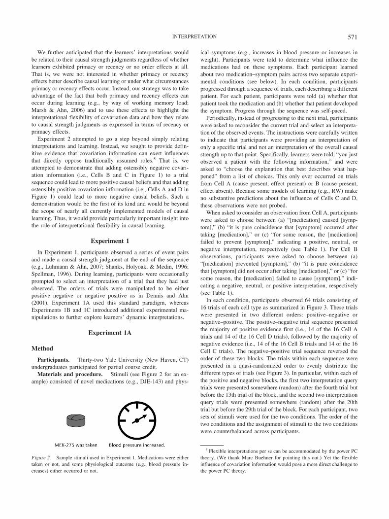
Materials and procedure. Stimuli (see Figure 2 for an ex-ample) consisted of novel medications (e.g., DJE-143) and phys-

ical symptoms (e.g., increases in blood pressure or increases inweight). Participants were told to determine what influence themedications had on these symptoms. Each participant learnedabout two medication–symptom pairs across two separate experi-mental conditions (see below). In each condition, participantsprogressed through a sequence of trials, each describing a differentpatient. For each patient, participants were told (a) whether thatpatient took the medication and (b) whether that patient developedthe symptom. Progress through the sequence was self-paced.

Periodically, instead of progressing to the next trial, participantswere asked to reconsider the current trial and select an interpreta-tion of the observed events. The instructions were carefully writtento indicate that participants were providing an interpretation ofonly a specific trial and not an interpretation of the overall causalstrength up to that point. Specifically, learners were told, “you justobserved a patient with the following information,” and wereasked to “choose the explanation that best describes what hap-pened” from a list of choices. This only ever occurred on trialsfrom Cell A (cause present, effect present) or B (cause present,effect absent). Because some models of learning (e.g., RW) makeno substantive predictions about the influence of Cells C and D,these observations were not probed.

When asked to consider an observation from Cell A, participantswere asked to choose between (a) “[medication] caused [symp-tom],” (b) “it is pure coincidence that [symptom] occurred aftertaking [medication],” or (c) “for some reason, the [medication]failed to prevent [symptom],” indicating a positive, neutral, ornegative interpretation, respectively (see Table 1). For Cell Bobservations, participants were asked to choose between (a)“[medication] prevented [symptom],” (b) “it is pure coincidencethat [symptom] did not occur after taking [medication],” or (c) “forsome reason, the [medication] failed to cause [symptom],” indi-cating a negative, neutral, or positive interpretation, respectively(see Table 1).

In each condition, participants observed 64 trials consisting of16 trials of each cell type as summarized in Figure 3. These trialswere presented in two different orders: positive–negative ornegative–positive. The positive–negative trial sequence presentedthe majority of positive evidence first (i.e., 14 of the 16 Cell Atrials and 14 of the 16 Cell D trials), followed by the majority ofnegative evidence (i.e., 14 of the 16 Cell B trials and 14 of the 16Cell C trials). The negative–positive trial sequence reversed theorder of these two blocks. The trials within each sequence werepresented in a quasi-randomized order to evenly distribute thedifferent types of trials (see Figure 3). In particular, within each ofthe positive and negative blocks, the first two interpretation querytrials were presented somewhere (random) after the fourth trial butbefore the 13th trial of the block, and the second two interpretationquery trials were presented somewhere (random) after the 20thtrial but before the 29th trial of the block. For each participant, twosets of stimuli were used for the two conditions. The order of thetwo conditions and the assignment of stimuli to the two conditionswere counterbalanced across participants.

5 Flexible interpretations per se can be accommodated by the power PCtheory. (We thank Marc Buehner for pointing this out.) Yet the flexibleinfluence of covariation information would pose a more direct challenge tothe power PC theory.

Figure 2. Sample stimuli used in Experiment 1. Medications were eithertaken or not, and some physiological outcome (e.g., blood pressure in-creases) either occurred or not.

571INTERPRETATION

After viewing the entire set of trials, participants rated the causalstrength of the medication by judging “the extent to which [med-ication] influences [symptom]” on a –100 (“[medication] pre-vented [symptom]”) to 100 (“[medication] caused [symptom]”)scale where 0 was labeled as “[medication] had no influence on[symptom].”

Results

Analyses of interpretations. As shown in Table 2, an aver-age of 61.9% of interpretations differed from the way classicmodels of causal induction use these trials to modify causal beliefs(i.e., bold values in Table 2, such as negative or neutral interpre-tations of Cell A or joint presence of cause and effect). Theseinterpretations occurred both for Cell A (M � 60.5%) and Cell B(M � 63.3%) and also across the positive–negative condition(M � 60.2%) and the negative–positive condition (M � 63.7%).Consistent with the expectation-based account, the inconsistentinterpretations tended to occur more frequently in the second block(M � 68.0%) than in the first block (M � 55.9%), presumablybecause people would have a stronger expectation by the time theycompleted observing the first block and moved into the secondblock. Below, we offer comparative analyses to show interpreta-tional flexibility.

To statistically evaluate participants’ interpretations, we recodedeach of the positive, negative, and neutral interpretation state-ments. Positive judgments (i.e., choosing Option a for Cell A and

Option c for Cell B; see the Method section above) were scored as1. Negative judgments (i.e., choosing Option c for Cell A andOption a for Cell B) were scored as 1. Neutral judgmentsappealing to pure coincidence were scored as 0. These scores,broken down by block and order, are shown in Figure 4. A 2(order: positive–negative vs. negative–positive) � 2 (block: firsthalf vs. second half) repeated measures analysis of variance(ANOVA) found no main effect of block but a significant maineffect of order, F(1, 31) � 57.30, p � .0001, and a significantinteraction effect, F(1, 31) � 98.97, p � .0001. Both of thesesignificant effects are explored further.

We first considered judgments made in the first half of the trialsequences (i.e., during the positive half of the positive–negativeorder and the negative half of the negative–positive order). If ourparticipants rigidly interpreted the covariation information, thenthese judgments should be equivalent because participants werealways asked to interpret identical observations (i.e., two from CellA and two from Cell B). To the contrary, they were significantlydifferent from each other, t(31) � 19.00, p � .0001. Whereasfirst-half interpretations in the positive–negative order were sig-nificantly greater than zero (M � .73, SD � .24), t(31) � 17.08,p � .0001, those in the negative–positive order were significantlyless than zero (M � .62, SD � .30), t(31) � 11.47, p � .0001.That is, interpretations diverged in the first block such that theywere generally consistent with the neighboring trials (a neighbor-hood effect henceforth).

However, second-half interpretations in the positive–negative(M � .007, SD � .50) and negative–positive (M � .02, SD �.47) orders did not differ from each other, t(31) � 0.11, ns, and didnot differ from zero: positive–negative, t(31) � 0.08, ns; negative–positive, t(31) � 0.28, ns. This result suggests that the neighbor-hood effects were negated by expectations derived from the firsthalf of the sequence. Thus, interpretations in a negative block weremore negative when presented in the absence of prior experiences(i.e., the first half of the negative–positive order) than whenpreceded by a positive block (as in the second half of the positive–negative order), t(31) � 5.51, p � .0001. Similarly, interpretations

Table 2Average Percentages of Choices for Each Interpretation inExperiment 1A

Condition and block Generative Neutral Preventive

Positive–negative conditionPositive block (first)

Cell A 93.75 6.25 0Cell B 53.13 45.31 1.56

Negative block (second)Cell A 28.13 54.69 17.19Cell B 23.44 40.63 35.94

Negative–positive conditionNegative block (first)

Cell A 0 57.81 42.19Cell B 0 18.75 81.25

Positive block (second)Cell A 35.94 39.06 25.00Cell B 12.50 59.38 28.13

Note. Frequencies in bold represent interpretations that are inconsistentwith the way classic causal learning models use covariation to modifycausal beliefs.

Figure 3. Trial sequences utilized in Experiment 1. The sequence wasconstructed as follows. Positive blocks began with two trials from Cell Aand two from Cell D (randomly ordered). These were then followed by aseries of eight trials: three each from Cells A and D and one each fromCells B and C (all eight randomly ordered). Within this eight-trial series,participants interpreted the B trial and one of the A trials, as indicated bycircles in the figure. This was then followed by another series of eighttrials: four each from Cells A and D (randomly ordered). These were thenfollowed by another series of eight trials: three each from Cells A and Dand one each from Cells B and C (all eight randomly ordered). Within thiseight-trial series, participants again were asked to interpret the A trial andone of the B trials, as indicated by circles in the figure. The sequence thenended with two observations from Cell A and two from Cell D (randomlyordered). The top portion of the figure summarizes the overall contingencycollapsed across the two blocks.

572 LUHMANN AND AHN

in a positive block were more positive when presented in theabsence of prior experiences (i.e., the first half of the positive–negative order) than when preceded by a negative block (as in thesecond half of the negative–positive order), t(31) � 7.77, p �.0001.

Relationship between interpretation judgments and causalstrength judgments. Next, we examined whether our learners’interpretation judgments were linked to their learning as suggestedby the expectation bias account. As shown in Figure 5, partici-pants’ judgments as a whole exhibited neither a primacy (e.g.,Dennis & Ahn, 2001) nor a recency effect (e.g., Lopez et al.,1998).6 Judgments were near zero in both the positive–negative(M � 5.56, SD � 35.99) and the negative–positive (M � 6.19,SD � 34.77) conditions and did not differ from each other, t(31) �.06, ns.

More importantly, we examined whether variance in individu-als’ causal strength judgments was related to variance in theirinterpretation judgments. Specifically, we evaluated whether theextent to which participants’ interpretations were consistent with

the first block correlated with the extent to which participants’causal strength judgments were consistent with the first block (i.e.,the amount of primacy effect).

To do so, we computed (a) the extent to which the first-blockinterpretations were consistent with the first-block observations(i.e., measure of the neighborhood effect) and (b) the extent towhich the second-block interpretations were consistent with thefirst-block observations (i.e., measure of the expectancy-basedeffect). Then, we examined the extent to which each of thesemeasures correlated with (c) the magnitude of the primacy effectsin participants’ causal strength judgments. Appendix B explainshow we computed these three measures, using concrete examples.Then, we performed a multiple regression analysis using (a) and(b) as predictors of (c). The results of this analysis indicate thatlearners’ interpretation judgments were highly predictive of theircausal strength judgments, F(2, 29) � 6.56, p � .005. Inspectionof the beta values reveals that it was only interpretations from thesecond block of the sequence that were related to causal strengthjudgments, t(29) � 2.51, p � .05; first-block interpretationsshowed no such relationship, t(29) � 1.53, p � .14. In otherwords, causal strength judgments were particularly related to howlearners reacted to the second, conflicting block of observations inthe order effect paradigm, rather than the neighborhood effectsfound in the first block. Those learners whose second-half inter-pretations were strongly consistent with the first block of thesequence also provided causal strength judgments that reflectedthe first block of the sequence. In contrast, learners whose second-half interpretations were consistent with the second block of thesequence tended to provide causal strength judgments that re-flected the second block of the sequence.

To illustrate the relationship between interpretation judgmentsand causal strength judgments more vividly, we performed amedian split of participants based on their causal strength score(Mdn � 1.25). This divides participants into those whose causalstrength judgments generally exhibited primacy and those whogenerally exhibited recency. Figure 4 displays the interpretationjudgments of these two groups. This graph illustrates how the twogroups’ interpretations differed. Those learners who exhibitedmore of a primacy effect provided second-half interpretation judg-ments that were more consistent with the first half of the trialsequence. In contrast, those learners who exhibited more of arecency effect provided second-half interpretations that were moreconsistent with the second half of the trial sequence.

Discussion

The current results suggest that people’s causal learning may nottreat covariation information statically, as traditionally imple-mented. Observations from Cell A, for example, were often inter-preted as being consistent with a preventative causal belief. Thus,it appears that people’s interpretations of covariation informationwere influenced by several factors other than the cells of thecovariation matrix. First, we observed neighborhood effects, inwhich interpretations were modulated by the observations in the

6 Any difference between the current results and those of Dennis andAhn (2001) may be attributable to the repeated interruption, which hasbeen shown to reduce the amount of primacy effect (Marsh & Ahn, 2006).

Figure 4. Experiment 1A interpretation results. Overall, participants ex-hibited neither recency nor primacy. Causal strength judgments did notdiffer depending on order. Interpretation judgments in the second half ofthe sequence show a similar pattern. Error bars represent 1 standard errorof the mean.

573INTERPRETATION

immediately surrounding sequence. Interpretations were more pos-itive in positive blocks and more negative in negative blocks.Second, we observed more long-ranging effects of prior experi-ence. The neighborhood effects observed early in learning wereeliminated when learners had acquired conflicting prior experi-ence.

One could argue that the participants were merely confusedabout the instructions and that, instead of providing an interpreta-tion of a given trial, they were providing an overall estimate ofcausal strength up to that point in the sequence. For instance,according to this account, the second-half interpretations in thepositive–negative order were made when the contingency was stillsomewhat positive (see Figure 3), which is why the second-halfinterpretations were somewhat positive. Disentangling such a pos-sibility from the expectation-based account is difficult because wefully expect that individual interpretations are made according tolearner’s current beliefs about the strength of the causal relation-ship. We address this issue more directly later in the article(particularly Experiments 1C and 2).

For the next two experiments (Experiments 1B and 1C), wefocused on the relationship between learners’ interpretation judg-ments and their subsequent causal strength judgments. We foundin Experiment 1A that our participants’ interpretation judgmentswere not arbitrary but were connected to their learning in aprincipled manner. Our next two experiments manipulated eitherinterpretation or causal strength judgments to see whether a similarrelationship would continue to hold.

Experiment 1B

Experiment 1B manipulated the extent to which causal strengthestimates are influenced by the presentation order of evidence. Asdiscussed in the introduction, both recency (Lopez et al., 1998) andprimacy (Dennis & Ahn, 2001) effects are possible, and therecency effect is more likely when learners’ working memory isoverloaded (Marsh & Ahn, 2006). The current experiment usedMarsh and Ahn’s (2006) finding to elicit a recency effect. Partic-ipants proceeded through a learning task as in Experiment 1A,

except that they were now required to perform a secondary task,designed to increase cognitive load, and thus induce a recencyeffect. As a result, we expected that the interpretation resultswould be similar to those of the participants who showed therecency effect in Experiment 1A (see Figure 4).

Method

Sixteen Yale University undergraduates participated for partial coursecredit. The stimuli and procedure were identical to Experiment 1A withone exception. While learners progressed through the trial sequence, theywere required to count backward, by threes, from a large number (e.g.,286) provided by the experimenter. The counting task was performedduring the entire learning sequence, including while making both inter-pretation and causal judgments. To ensure compliance, learners countedaloud and were told ahead of time that their counting would be monitoredby experimenter stationed in an adjacent room (well within earshot).

Results and Discussion

When participants were required to perform a difficult second-ary task, we observed a robust recency effect (see Figure 6).Causal strength judgments in the positive–negative order (M �11.94, SD � 33.00) were much lower than the judgments in thenegative–positive order (M � 19.25, SD � 29.68), t(15) � 2.54,p � .05. The critical question was whether this manipulation alsoinfluenced learners’ interpretations.

Table 3 illustrates learners’ interpretation judgments, again bro-ken down by order and block. An average of 63.5% of interpre-tations were inconsistent with traditional role of covariation infor-mation (i.e., bold values in Table 3). Such interpretations occurredboth for Cell A (M � 59.8%) and for Cell B (M � 67.2%), acrossthe positive–negative condition (M � 63.8%) and the negative–positive condition (M � 63.3%), and in both the first block (M �58.6%) and the second block (M � 68.5%).

For more fine-level statistical analyses, the three types of judg-ments were scored as before (positive � 1, negative � 1,neutral � 0), and the mean scores for each order, broken down by

Figure 5. Interpretations after performing a median split on learners’ causal strength judgments. Those in theprimacy group exhibited greater primacy effect (more positive in the positive–negative condition and morenegative in the negative–positive condition). Those in the recency group tended to exhibit the opposite pattern.Error bars represent 1 standard error of the mean.

574 LUHMANN AND AHN

block, are shown in Figure 6. A 2 (order: positive–negative vs.negative–positive) � 2 (block: first half vs. second half) repeatedmeasures ANOVA found both a significant main effect of order,F(1, 15) � 10.00, p � .01 and an interaction between order andblock, F(1, 31) � 81.08, p � .0001. As in Experiment 1A,interpretations during the first half of the sequence were consistentwith the local context (a neighborhood effect) and thus differedacross the two orders, t(15) � 6.71, p � .0001.

Where the current results diverge from Experiment 1A is in thesecond-half interpretations. Recall that, in Experiment 1A, second-half interpretations were near zero and identical across the twoorders. In contrast, second-half interpretations in the positive–negative order (M � .08, SD � .22) were significantly lowerthan those in the negative–positive order (M � .23, SD � .28),t(15) � 3.18, p � .01. That is, we observed neighborhood effectsin the second half of the sequence; second-half interpretation

judgments were consistent with the evidence contained in thesecond half of the trial sequence.

Thus, using a dual-task paradigm to induce a recency effect inlearners’ causal strength judgments, participants’ interpretationjudgments in the second block became less affected by the infor-mation presented in the first block. Learners in the positive–negative order made more negative interpretations in the secondhalf and then provided primarily negative causal strength judg-ments. Learners in the negative–positive order made more positiveinterpretations in the second half and then provided primarilypositive causal strength judgments.

Finally, we examined more directly the relationship between individ-ual learners’ interpretations and their causal strength judgments. As inExperiment 1A, we computed the extent to which interpretations andcausal strength judgments were expectancy based, using the compositescores for each judgment (see Appendix B). These scores were thenentered into a multiple regression model with participants’ causal strengthjudgments as the dependent variable. Just as in Experiment 1A, causalstrength judgments were strongly predicted by the extent to which thesecond-half interpretations were consistent with the first-half covariation,t(13) � 2.57, p � .05, but not by the extent to which the first-halfinterpretations were consistent with the first-half covariation, t(13) � 1.This result suggests that, despite modulating both causal strength andinterpretation judgments, the secondary task did not eliminate the rela-tionship between these judgments. That is, even with our experimentalmanipulation, we continued to observe a reliable relationship betweenindividuals’ interpretations, particularly those in the second half of thesequence, and causal strength judgments. This again suggests that there isa strong connection between the processes that underlie interpretation andlearning.

Experiment 1C

Experiment 1C modulated learners’ interpretations, instead ofcausal strengths. We introduced novel causes during specific,contradictory observations. For example, in the second half of anegative–positive sequence, observations from Cell A (i.e., cause

Table 3Average Percentages of Choices for Each Interpretation inExperiment 1B



Cell A 71.88 28.13 0Cell B 43.75 50.00 6.25

Negative block (second)Cell A 13.33 73.33 6.67Cell B 16.67 36.67 40.00


Cell A 18.75 46.88 34.38Cell B 6.25 25.00 68.75



Figure 6. Experiment 1B results. Overall, participants exhibited recencyeffects. Causal strength judgments were more negative in the positive–negative condition and more positive in the negative–positive condition.Interpretation judgments in the second half of the sequence show a similarpattern. Error bars represent 1 standard error of the mean.

575INTERPRETATION

present, effect present) were accompanied by a second, novelcause. Although the causal role of this second cause was leftambiguous, its addition was intended to bias the interpretation lentto these observations such that learners would be more likely tochoose the negative, “for some reason, the [medication] failed toprevent [symptom]” interpretation. Unlike the preceding experi-ments, the novel cause should provide learners with a salientexplanation or an excuse for the aberrant observation, essentiallytransforming the abstract “for some reason” into something ratherconcrete. We expected that this modification would lead to second-half interpretations even more consistent with the first half of thesequence. As a result, we also predicted that causal strengthjudgments would also exhibit greater primacy.

Method

Seventeen Yale University undergraduates participated for par-tial course credit. The stimuli and procedure were similar toExperiment 1A with a few exceptions. Participants were presentedwith information about two medications simultaneously. Partici-pants were told that their task was to learn about only one of thetwo causes, the target cause, and that they would not have to judgethe other cause, the alternative cause. The target cause behaved asin Experiment 1A (see Figure 3). The alternative cause was onlypresent in the second half of the trial sequence and then onlyduring observations that were inconsistent with the first block andon which the target cause was present. Thus, the alternative causewas present during all observations from Cell B in the negativehalf of the positive–negative order and during all observationsfrom Cell A in the positive half of the negative–positive order.

The alternative cause was introduced in the second half, oninconsistent trials, to modulate learners’ interpretations so as toreflect the first half of the trial sequence more than the second half.For instance, after observing the first half of the positive–negativeorder and developing the expectation that there is a positive causalrelationship, observing the target cause and the alternative cause inthe absence of the effect (i.e., Cell B) is likely to elicit theinterpretation that the alternative cause is to be blamed for thefailure to produce the effect. We predicted that our experimentalmanipulations of learners’ interpretation judgments would alsoelicit more expectation-based causal strength judgments.


Table 4 shows the mean percentage of choices for interpretationjudgments. As before, a bulk of trials (M � 62.13%) were notinterpreted as traditionally implemented. Such interpretations fre-quently occurred for both Cell A (M � 58.8%) and Cell B (M �65.4%), across the positive–negative order (M � 55.1%) and thenegative–positive order (M � 69.1%), and for both the first block(M � 60.3%) and the second block (M � 64.0%).

Figure 7 shows participants’ mean interpretation scores (1 �positive, 0 � neutral, 1 � negative). A 2 (order: positive–negative vs. negative–positive) � 2 (block: first half vs. secondhalf) repeated measures ANOVA revealed a significant main ef-fect of order, F(1, 15) � 29.01, p � .0001, but no interactionbetween order and block, F(1, 32) � 1, ns. First-half interpreta-tions were again consistent with the surrounding context. Those inthe positive–negative order were significantly greater than zero

(M � .59, SD � .31), t(16) � 7.94, p � .0001, whereas those inthe negative–positive order were significantly less than zero (M �.49, SD � .42), t(16) � 4.78, p � .0001. In contrast, second-halfinterpretations were overwhelmingly consistent with the first half ofthe trial sequence (and thus inconsistent with the surrounding con-text). Second-half judgments from the positive–negative order weresignificantly greater than zero (M � .57, SD � .38), t(16) � 6.18, p �.0001, whereas judgments from the second half of the negative–positive order were significantly less than zero (M � .50, SD �.47), t(16) � 4.41, p � .0005. Averaging across blocks, the overalldifference between the two orders was also significant, t(16) � 8.46,p � .0001, suggesting that our manipulation had the desired effect onlearners’ interpretations. The critical question was whether this ma-nipulation would also influence learning as measured by participants’causal strength judgments.

As can be seen in Figure 7, participants’ causal strength judgmentsexhibited a strong primacy effect. Causal strength judgments in thepositive–negative order were significantly greater than zero (M �45.41, SD � 28.11), t(16) � 6.66, p � .0001, whereas judgments inthe negative–positive order were significantly less than zero (M �31.35, SD � 35.98), t(16) � 3.59, p � .005. The differencebetween two orders was significant, t(16) � 8.06, p � .0001.

Finally, using multiple regression over the composite scores forinterpretation judgments and causal strength judgments as ex-plained in Experiment 1A and Appendix B, we again testedwhether individuals’ interpretations would predict their causalstrength judgments. Just as in the previous two studies, causalstrength judgments were predicted by the extent to which second-half interpretations were consistent with the first block, t(14) �2.32, p � .05, but not by the extent to which the first-halfinterpretations were consistent with the first block, t(14) � 1.

To summarize, by providing an excuse, participants could morereadily explain away aberrant trials in the second block, and wefound much stronger expectancy-based interpretations in the sec-ond block. At the same time, participants’ causal strength judg-ments reflected the first half of the sequence even more than thesecond half.

Table 4Average Percentages of Choices for Each Interpretation inExperiment 1C



Cell A 91.18 5.88 2.94Cell B 38.24 52.94 8.82

Negative block (second)Cell A 67.65 32.35 0Cell B 58.82 29.41 11.76


Cell A 0 52.94 47.06Cell B 8.82 32.35 61.76



576 LUHMANN AND AHN

Experiment 1C also undermines one possible alternative account toour claim that interpretations derive causal strength judgments. Thiscounterargument claims that the interpretation judgments merely re-flect �P experienced so far, or causal power (Cheng, 1997) estimatedup to that point. For instance, by the time participants provided the lastinterpretation judgments in the first block, the overall �P and causalpower were about 0.71 and 0.83, respectively, in the positive–negative sequence and 0.71 and 0.83, respectively, in thenegative–positive sequence. By the time they provided the last inter-pretation judgments in the second block, the overall �P and causalpower were about 0.07 and 0.13, respectively, in the positive–negative sequence and about 0.07 and 0.13, respectively, in thenegative–positive sequence. Thus, the difference between the twoorders became smaller by the time participants experienced the sec-ond block, which mirrors the interpretation judgments observed inExperiments 1A and 1B. In Experiment 1C, we used identical trials(i.e., identical �P and causal power), but the interpretation results

observed in Experiment 1C do not at all reflect this reduced differencebetween the two conditions in the second block. Although the cova-riation between the target cause and the effect dramatically changed inthe second half of the sequence, just as in Experiments 1A and 1B, theinterpretation judgments from the first and the second halves wereindistinguishable.

Experiment 2

Experiment 1 demonstrated that observations from Cell A can beinterpreted as evidence for an inhibitory causal relationship and thatobservations from Cell B can be interpreted as evidence for a gener-ative causal relationship. Experiment 2 tested a stronger version of ourproposal; Cell A can act to decrease a causal strength and Cell B canact to increase a causal strength. That is, covariation information canexert influences on overall causal strength judgments in ways thatoppose traditionally implemented roles.

The design is illustrated in Figure 8. In the control conditions,the sequence consisted of two blocks (one positive and one neg-ative), but the second block contained 10 fewer trials than inExperiment 1 (see the trials without brackets in Figure 8). Morespecifically, the control condition of the positive–negative se-quence contained five fewer B and five fewer C trials in the secondhalf, making the overall contingency positive (�P � 0.2). Simi-larly, the control condition of the negative–positive sequence con-tained five fewer A and five fewer D trials in the second half,making the overall contingency negative (�P � 0.2). In theexperimental conditions, the positive–negative and negative–positive sequences were identical to Experiment 1 (except foralternative causes; see below). Thus, the overall contingency ofeach sequence was zero.

Importantly, in the experimental conditions, on these extra ob-servations (i.e., the bracketed trials in Figure 8), a second, alter-native cause was present. As in Experiment 1C, these were in-serted to elicit more nontraditional interpretations of covariationinformation by reminding learners that there may be alternativecauses that can be blamed for aberrant observations.

According to many traditional models of causal learning, in-cluding RW, �P, and power PC, judgments after the positive–negative sequence should be more negative in the experimentalcondition than in the control condition, and judgments after thenegative–positive sequence should be more positive in the exper-imental condition than in the control condition. For �P and powerPC, this is because �P is 0 for both sequences in the experimentalcondition, whereas, in the control condition, �P is 0.2 and 0.2 ofthe positive–negative and negative–positive sequences, respec-tively (see Figure 8 for the summary). One may argue that pres-ence of alternative causes may create a distinctive context and thata learner might conditionalize on the presence or absence ofalternative causes (e.g., Spellman, 1996). If participants treat trialswith alternative causes separately or ignore them, �P and powerPC predict that the control and experimental conditions are iden-tical. However, these models can never predict that the experimen-tal condition of the positive–negative sequence, which containsmore B and C trials than its control condition, would result inhigher causal judgments than its control condition. Likewise, theycan never predict that the experimental condition of the negative–positive sequence, which contains more A and D trials than its

Figure 7. Experiment 1C results. Causal strength judgments were morepositive in the positive–negative condition and more negative in thenegative–positive condition. Interpretation judgments in the second half ofthe sequence show a similar pattern. Error bars represent 1 standard errorof the mean.

577INTERPRETATION

control condition, would result in lower causal judgments than itscontrol condition.

RW makes similar predictions. The experimental condition con-tains more B and C trials in the second half than the controlcondition, and therefore, regardless of the parameter values, thefinal associative strength of the experimental condition can neverbe higher than that from the control condition of the positive–negative sequence. Similarly, RW would never predict the controlcondition of the negative–positive sequence to be lower than thatfrom its experimental condition.

In contrast, we predicted that the exact opposite would occur.Suppose a learner is progressing through a positive–negative se-quence. The first half of the sequence creates a belief that the causeis strongly generative in nature. When encountering the second,negative half of the sequence, learners in the control condition willprocess this negative information in light of their existing hypoth-esis, blunting this information’s influence. Learners in the exper-imental condition will be confronted with even more negativeevidence. However, some of this evidence will occur in the pres-ence of an alternative cause, allowing learners to interpret theseobservations as being consistent with their existing, positive hy-

pothesis (e.g., Experiment 1C). We further expected that the pres-ence of an alternative cause on these few trials would encouragesimilar interpretations of B and C trials without alternative causesthroughout the remainder of the sequence (or perhaps retrospec-tively), ultimately leading to more positive beliefs. The oppositewould occur with the negative–positive sequence. Thus, addingobservations that, according to the traditional accounts, contradictthe initial observations may be able to paradoxically reinforcelearners’ initial hypothesis.

Method

Participants. Forty-four Stony Brook University (StonyBrook, NY) undergraduates participated for partial course credit.

Materials and procedure. The stimuli and procedure weresimilar to those used in Experiment 1, although participants wereno longer asked to provide interpretations. Stimuli consisted ofnovel medications (e.g., DJE-143), each of which could have somecausal influence on granulocytes (described as “a substance pro-duced in people’s blood”). Participants were told that it was theirjob to determine what influence the medications had on granulo-

Figure 8. The design of Experiment 2. The control condition included sequences with slightly longer firsthalves so that the overall covariation (�P) would be more reflective of the evidence presented at the beginningof the sequence than the evidence presented at the end. The experimental condition added additional observationsto the second half of the sequences (placed in brackets). These additional observations also included a second,alternative cause (see text for further details). Importantly, these extra observations changed the overallcovariation of both sequences to be zero.

578 LUHMANN AND AHN

cytes. Each participant was again exposed to two different trialsequences, each of which instantiated two different orders:positive–negative and negative–positive. Figure 8 shows the actualfrequencies and sequences. The trials within each sequence werepresented in a quasi-randomized order to evenly distribute thedifferent types of trials.

The critical manipulation in Experiment 2 occurred during thesecond half of each sequence. Participants in the control conditionreceived sequences consisting of trials without brackets in Fig-ure 8. In contrast, participants in the experimental condition re-ceived an additional 10 observations in the second half of thesequence (i.e., bracketed trials in Figure 4). The experimentalcondition of the positive–negative sequence included five addi-tional Cell B trials and five additional Cell C trials presented in thesecond half of the sequence, and the experimental condition of thenegative–positive sequence included five additional Cell A trialsand five additional Cell D trials presented in the second half of thesequence. (These additional trials made the sequences of the ex-perimental conditions identical to those in Experiment 1.) On theseextra trials, a second, alternative cause was also always present.This alternative cause was not mentioned on any other trials duringthe sequence (i.e., not explicitly present, not explicitly absent). Tomake sure that all learners (in both conditions) had equivalentexpectations about alternative causes for the trials that were sharedbetween the two conditions, the initial task instructions specified,“If we know whether a given patient is taking other medication,that information will be presented to you. If there is no informationabout other medication, the patient may or may not be taking othermedication, we simply don’t know.”

After viewing the entire set of trials, all participants rated thecausal strength of the medication. Specifically, participants wereasked to, “judge the extent to which [medication] influences gran-ulocytes.” Responses could range from –100 (“[medication] pre-vented granulocytes”) to 100 (“[medication] caused granulo-cytes”), with 0 labeled as “[medication] had no influence ongranulocytes.”

The manipulation of the experimental and control conditionswas a between-subject variable (N � 22 in each condition) and theorder (positive–negative vs. negative–positive sequence) was awithin-subject variable. For each participant, a differentmedication–symptom pair was utilized in the two different ordersequences. The two orders and the assignment of stimuli werecounterbalanced across participants.


Figure 9 shows the results. A 2 (experimental vs. control) � 2(order) ANOVA with repeated measure on the latter factor founda significant main effect of order, F(1, 82) � 13.66, p � .0005,and, more critically, a significant interaction effect, F(1, 82) �12.99, p � .001. As predicted, this interaction was obtainedbecause the positive–negative sequence elicited more positivejudgments in the experimental condition (M � 55.73, SD � 28.94)than in the control condition (M � 25.23, SD � 39.05), t(42) �2.93, p � .01, whereas the negative–positive sequence elicitedmore negative judgments in the experimental condition (M �43.91, SD � 34.02) than in the control condition (M � 24.36,SD � 28.84), t(42) � 2.05, p � .05.

This pattern conforms to our predictions and provides strongevidence that the four covariation evidence types do not alwaysexert the traditional influence on learning. Adding observations onwhich the target cause was present and the effect was absent (CellB) and observations on which the target cause was absent and theeffect was present (Cell C) resulted in more generative causalstrength judgments. Conversely, adding observations on which thetarget cause and effect were both present (Cell A) and observationson which the target cause and effect were both absent (Cell D)resulted in more preventative causal strength judgments.7

7 One may argue that the additional trials marked with potential alter-native cues could have implied a change in context. One possibility is thatparticipants could have believed that only the trials with potential alterna-tive cues had different contexts. As discussed at the beginning of Experi-ment 2, however, if only these trials were ignored by the participants, theexperimental and the control conditions would be equivalent, so thispossibility cannot account for the current results. The second possibility isthat the occasional presence of a potential alternative cause could haveresulted in the wholesale ignorance of the second half of the sequences. Inthis case, the causal powers according to power PC in the first half of thesequences would be 0.86 in the positive–negative sequence and 0.86 inthe negative–positive sequence. The results from both Experiment 1C (0.45and 0.31, respectively) and the experimental condition of Experiment 2(0.55 and 0.43, respectively) deviate substantially from these predictions.Furthermore, the judgments deviate in the direction (toward zero) thatwould be expected if learners did in fact processes the second halves ofthese sequences. Last, we note that previous authors (e.g., Glautier, 2008)have suggested that a change in context might explain recency effects incausal learning. That is, these authors proposed that a change in contexthalfway through a learning sequence would cause learners to ignore thefirst half (rather than the second half, as suggested by a reviewer). Giventhe amount of disagreement between these various accounts, future workwill be needed to more thoroughly explore the relationship between them.

Figure 9. Experiment 2 results. The experimental condition added ob-servations to the second half of each sequence (additional observationsfrom Cells B and C in the positive–negative sequence and additionalobservations from Cells A and D in the negative–positive sequence). Thesolid circles represent the predictions of the �P model (causal powerpredictions are similar). As can be seen, the pattern exhibited by �Pindicates that the addition of Cell B and C observations will lower causalstrength judgments and that the addition of Cell A and D observations willraise causal strength judgments. Participants exhibited the opposite pattern.Error bars represent 1 standard error of the mean.

579INTERPRETATION

General Discussion

We have suggested that an integral part of causal learning is thesubjective processing of individual pieces of covariation informa-tion. The current study sought to provide support for this proposalin two ways. In Experiment 1, we had learners provide explicitinterpretations during the course of learning. These results illus-trate several important points. First, interpretations of identicalobservations varied depending on the immediately surroundingcontext. For example, interpretations made in the midst of astrongly positive block were more positive than interpretations ofidentical observations made in the midst of a strongly negativeblock. Second, interpretations varied depending on the expecta-tions learners developed at the beginning of learning. For instance,learners interpreted observations more negatively if learners hadpreviously encountered a strongly negative sequence of observa-tions than if they had not. Last, we found that these interpretationswere systematically related to causal strength judgments. Individ-ual learners’ interpretations idiosyncratically predicted their ownstrength judgments. In addition, we found interpretations andcausal strength judgments to be linked at the group level usingexperimental manipulations designed to modulate causal strengthjudgments (Experiment 1B) and interpretations (Experiment 1C).

In Experiment 2, we went even further and demonstrated thatthe addition of supposedly positive covariation information couldresult in more negative causal strength judgments and vice versa.Compared to the control conditions, the experimental conditionshad a small number of extra trials that were inconsistent with thefirst half of the sequence and included a second, alternative cause.The presence of the alternative cause allowed learners to interpretthese observations in a way that was consistent with their existinghypotheses (e.g., Experiment 1C). Presumably, because of theseunconventional interpretations, causal strength judgments werealtered in ways that did not correspond to the assumptions oftraditional learning theories. This experiment is the first empiricaldemonstration that additional presentation of Cells B and C canresult in more generative causal strength judgments and that ad-ditional presentation of Cells A and D can result in more preven-tative causal strength judgments.

The current study helps to explain previous reports of primacyeffects in causal learning (Chapman & Chapman, 1969; Dennis &Ahn, 2001; Yates & Curley, 1986). Our results demonstrate thatthe hypotheses learners carry with them influence their interpre-tations, which, in turn, bias the changes that learners make to theirhypotheses. Learners who have just observed a set of evidencesuggesting a strong, generative causal relationship process subse-quent evidence differently than learners who have different priorexperience. This processing, under many conditions, operates suchthat evidence is processed to be consistent with the learner’scurrent expectations. Such expectation-based processing acts toattenuate the influence of subsequent, conflicting evidence andtends to yield primacy effects.

Our results further explain the dependence of primacy effects onworking memory (Marsh & Ahn, 2006), since working memory isrequired for expectations to fully influence the interpretation pro-cess. Without access to working memory, interpretations no longerbias data to be consistent with previously established expectations,and subsequent causal strength judgments reflect the relativelyunbiased, recent data. Thus, despite the variety of order effects we

observed in the current experiments (primacy, recency, and noorder effect at all), our data suggest that they may all be explainedwith a single process.

Token Versus Type Causal Cognition

One aspect of causal cognition that has received surprisinglylittle attention is the relationship between reasoning about causaltokens and causal types. Causal types are those causal beliefs thatdescribe a generality: Coffee causes alertness. This is the sort ofcausal belief that is typically explored in causal learning paradigms(Shanks et al., 1996). Causal tokens are those causal beliefs thatdescribe a specific causal interaction taking place in a specific timeand place: This morning’s coffee made me alert. This is the sort ofbelief that is typically labeled as causal reasoning (Goldvarg &Johnson-Laird, 2001; Wolff, 2007; Wolff & Song, 2003) and isoften framed as a problem to be solved (e.g., why are you alert thismorning?). Despite having two separate literatures, there is noparticular reason to think that reasoning about types and reasoningabout tokens are unrelated.

The causal strength judgments our learners made after observingthe entire sequence of observations were designed to elicit beliefsabout the causal type. That is, these judgments asked about thecausal pattern that held in general. The interpretations that learnersmake about individual trials are beliefs about the causal token. Forexample, the interpretation judgments in Experiment 1 asked for acausal description of a single episode. The neighborhood effectsand the effect of order on interpretation judgments found in Ex-periment 1 suggest that learners’ beliefs about causal types influ-enced their interpretation of the causal interactions on individualtrials. Consistent with this, we observed that interpretation judg-ments, particularly those in the second half of the sequence,predicted subsequent causal strength judgments across individuals,possibly suggesting a mutual influence of type and token process-ing.

Last and perhaps most interesting, Experiment 2 strongly sug-gests that the interpretation of individual observations can influ-ence causal strength judgments. In this experiment, we providedlearners with a select number of trials in which an alternative causewas present. These trials were specifically designed to bias thecausal explanation given to individual observations; learnerswere given an opportunity to excuse evidence that, according tothe traditional interpretation of covariation information, contra-dicted the first half of the learning sequence. Our results dem-onstrate that, when given this opportunity, learners used thealternative cause to interpret the seemingly contradictory ob-servations in atypical ways. As a result, these trials did notinfluence learners’ subsequent causal strength judgments in themanner that has been traditionally assumed.

Given these results, we argue that the processing of causal typesand the processing of causal tokens exert mutual influence on eachother. This suggests that the processes that underlie what is gen-erally labeled as causal reasoning and those that underlie causallearning may be heavily intertwined. This is a relationship that iscurrently absent from nearly all current causal learning models.One exception is our recent model, BUCKLE (bidirectional unob-served cause learning; Luhmann & Ahn, 2007), which describeshow people learn about causes that they cannot observe. Accordingto BUCKLE, learners engage in causal reasoning on each trial in

580 LUHMANN AND AHN

an attempt to overcome missing information. Learning then oper-ates by using the results of the causal reasoning as a replacementfor the missing information. Our results suggest that somethingsimilar was going on in the current study. Instead of trying to figureout whether causes were present or absent, learners in the currentstudy appear to have been engaged in generating explanations forindividual observations. As in BUCKLE, conclusions drawn aboutindividual observations apparently influenced subsequent learning. Ofcourse, we do not currently have any theories about how learningmight use explanations or interpretations as input because it has beenassumed that unprocessed covariation is sufficient to capture learningbehavior. Further work on this topic has the ability to both enrich andunify an understanding of causal learning, causal reasoning, and therelationship between these abilities.

Bayesian Inference

As discussed earlier, the two sets of classical models of learningcannot readily account for all aspects of our current results. What sortof process might explain both the interpretations and causal strengthjudgments we have reported here? A Bayesian approach seems im-mediately attractive. The hallmark of Bayesian inference is the abilityto integrate newly observed data with existing beliefs or hypotheses.Here, we briefly review several of the most recent Bayesian models ofcausal learning, discuss their important theoretical contribution, andexplain how they relate to our current findings.

Griffiths and Tenenbaum (2005) suggested that learners do notattempt to determine the strength of individual causal relationshipsbut rather attempt to determine whether there exists a causalrelationship (of any strength) between the potential cause and thepotential effect. For example, when asked to evaluate the degree towhich carbon dioxide causes global warming, Griffiths and Te-nenbaum suggested that people’s judgments can be thought toreflect a decision between a model of the world in which these twovariables are causally connected and a model of the world in whichthe two variables are unrelated. To test this proposal, Griffiths andTenenbaum formalized their proposal with a Bayesian modelcalled causal support and fit the model to several data sets. Eachset of data was collected by presenting a homogeneous set ofpositive covariation information to participants and eliciting causalstrength judgments. The results demonstrated that, across data sets,participants’ judgments tended to exhibit variability even whenother models (e.g., power PC and �P) would suggest they shouldbe constant. In general, the causal support model was able toaccount for many of these apparent deviations and provided betteroverall fits to the data.

Lu, Yuille, Liljeholm, Cheng, and Holyoak (2008) proposed aBayesian extension of Cheng’s power PC theory (Cheng, 1997).They proposed that people expect causes to be both necessary andsufficient to bring about their effects. That is, it is suggested thatpeople have an aversion to causes that are not systematicallyfollowed by their effects (sufficiency) and an aversion to effectsthat are not systematically preceded by their causes (necessity).Lu, Yuille, et al. formalized this expectation as a set of Bayesianpriors and compared the resulting model with an identical modelhaving no preference for necessity or sufficiency (which is essen-tially just causal power as described by Cheng, 1997). The twomodels were then fit to two types of data. The first type of data wascollected by presenting participants with homogeneous covariation

information and then eliciting causal strength judgments. When thetwo models were fit to the causal strength judgments, there waslittle difference between the model that preferred necessity andsufficiency and the model that had no preference. The second typeof data was collected by presenting participants with homogeneouscovariation information and eliciting judgments of causal structure(cf. Griffiths & Tenenbaum, 2005). Here, the model that expectednecessity and sufficiency provided significantly better fits to avariety of causal structure judgments.

Both Griffiths and Tenenbaum (2005) and Lu, Yuille, et al.(2008) put forth formal, Bayesian accounts of how covariationinformation is used to produce causal judgments. However, thecausal support model was explicitly designed to model judgmentsof causal structure (rather than causal strength, which was elicitedin the current study), and the prior expectation about necessity andsufficiency proposed by Lu, Yuille, et al. was only required toaccount for judgments of causal structure. Because of the focus oncausal structure rather than causal strength and because both ofthese models focus on aggregate covariation data rather thanindividual pieces of covariation information, these models are notimmediately applicable to the methods utilized in the current studyor the order effects found in the current study.

Recently, there have been two models proposed (Lu, Rojas, etal., 2008; Lucas & Griffiths, 2010) that are much more related, atleast in spirit, to the current study. Each of these models suggeststhat participants simultaneously learn two related things fromcovariation information. Learners must first determine how mul-tiple causes combine their influence to bring about their effects.For example, causes may combine their effects additively as is thecase when one takes two aspirin; two aspirin are twice as effectiveas one aspirin. Alternatively, causes may interact, as is the casewhen one mixes bleach and ammonia; despite neither being par-ticularly dangerous on its own, the combination is highly toxic. Onthe basis of their beliefs about how causes combine their influence,learners must also determine the strengths of the various causes.

To evaluate these proposals, the authors applied them to exper-iments in which learners received two sets of covariation informa-tion. In the first, training phase, learners received data that pro-vided hints as to how causes combined their influence to producetheir effects. For example, one experimental condition includedtraining data that, like the bleach and ammonia example, describeda pair of causes that each failed to produce the effect on its own butthat were able to produce the effect when paired together. Anothercondition included training data that, like the aspirin example,described a pair of causes that each produced the effect on its ownand also produced the effect when paired together. To evaluate theinfluence of the training, all learners were then provided with anidentical set of covariation information and asked to make causalstrength judgments. Despite making causal strength judgmentsabout identical covariation information, the different training con-ditions led to different causal judgments. For example, if onelearned that causes do not interact (like aspirin), then observing asingle cause that is not followed by its effect (i.e., Cell B) wouldsuggest that that cause was not particularly strong. If one hadinstead learned that causes do interact (like bleach and ammonia),then seeing the same observation (e.g., ammonia not being dan-gerous) would leave its interactive causal strength ambiguous.

These more recent proposals (Lu, Rojas, et al., 2008; Lucas &Griffiths, 2010) describe a more sophisticated formal account

581INTERPRETATION

(so-called hierarchical Bayesian inference) about how people ex-tract causal beliefs from covariation information. Just as has beendemonstrated in the current study, these models exhibit significantflexibility in how covariation information leads to causal beliefs.Specifically, these models are able to reach different causal con-clusions based on identical covariation information. The flexibilityexhibited by these models is directly tied to their assumption thatpeople simultaneously learn how causes interact to produce theireffects and learn causal strengths. Because a critical component ofthese models involves learning about how multiple causes com-bine their influence, however, they cannot be directly applied tothe current study (which only ever had participants learning abouta single cause). Yet these models clearly illustrate how the hier-archical Bayesian approach to causal learning can lead to a sig-nificantly greater flexibility than traditional models.

So far, we have reviewed a recent crop of Bayesian models thathave each described substantially more sophisticated processes bywhich covariation information is transformed into causal beliefs.Although each of these models relies on prior beliefs to dictateexactly how causal learning proceeds, the specific models thathave been proposed are not immediately applicable to our resultsfor a variety of reasons. Below, we provide more general discus-sion of the reasons for the limitations.

First, as explained in the earlier results, much of the flexibilitywe observed in the current study seems to have been a conse-quence of a strong relationship between beliefs about types (e.g.,does this cause produce the effect in general?) and beliefs abouttokens (e.g., did this cause produce the effect on this occasion?).The flexibility exhibited by the newer Bayesian models is a con-sequence of beliefs about causal strength (type) and beliefs at amore abstract level. Griffiths and Tenenbaum’s (2005) causalsupport model relies on beliefs about potential causal structure, Lu,Yuille, et al. (2008) modeled prior beliefs about the necessity andsufficiency of causes, and both Lucas and Griffiths (2010) and Lu,Rojas, et al. (2008) modeled beliefs about how causes interact. Toaccount for the results of Experiment 1, focus would instead haveto be directed to beliefs at a more specific (i.e., token) level.

Second, our results demonstrate the influence of a variety ofdifferent kinds of prior beliefs, and it is not yet clear how the entireset could be implemented within the Bayesian framework. Learn-ers’ interpretations were influenced by the proximal context, whatwe refer to as neighborhood effects. Observations surrounded bypredominately negative covariation information tended to bejudged negatively, whereas observations surrounded by predomi-nately positive covariation information tended to be judged posi-tively. In addition, learners’ interpretations were influenced by thedistal context. Observations preceded by a large block of negativecovariation information tended to be judged negatively, whereasobservations preceded by a large block of positive covariationinformation tended to be judged positively. These factors embodyexactly the sort of influences used by Bayesian inferences butsuggest that a process account will be necessary to fully accountfor our results. There have been Bayesian accounts of causallearning that attempt to account for the trial-by-trial dynamics oflearning (e.g., Danks, Griffiths, & Tenenbaum, 2003; Lu, Yuille, etal., 2008), but many of these are extremely simplistic, typicallyapplying standard inference iteratively after each trial. Only theproposal of Lu, Rojas, et al. (2008) exhibits the degree of sophis-tication likely necessary to deal with the current data.

The third factor is much more psychological in nature. InExperiment 1B, participants placed under cognitive load continuedto be influenced by the local context but were not particularlysensitive to the more long-ranging influence of the preceding blockof trials. To integrate this factor into a Bayesian account, one couldpresumably posit a resource-dependent process that is responsiblefor combining prior beliefs with current data. For example, simplyholding prior beliefs in memory may be cognitively taxing andthus be compromised in individuals or situations where workingmemory is compromised.

Impression Formation

Our theorizing about the order effect paradigm has been sub-stantially informed by prior work on impression formation. Inparticular, the order effect paradigm itself was taken from workoriginally done on impression formation (Asch, 1946). The para-digm is completely analogous to the current Experiment 1; thepresentation order of identical sequences of information is manip-ulated without changing the information itself. Much like thecurrent results, Asch’s (1946) findings demonstrated the influenceof prior expectations. If one’s first experience with a stranger ispredominantly positive, one will tend to overlook subsequentnegative experience and judge the individual to be relativelypositive, whereas the reverse presentation order will lead to rela-tively negative judgments (Asch, 1946). The similarity betweenthe primacy effects reported in impression formation and causallearning is striking. Interestingly, there have also been reports ofrecency effects in impression formation tasks using an order effectparadigm. One factor that appears to partly determine whether oneobserves primacy or recency is the frequency with which partici-pants are required to make judgments of the person under scrutiny(Stewart, 1965). Studies requiring more frequent judgments tend toreport recency, whereas those that elicit judgments only at the endof the sequence tend to report primacy. Interestingly, this exactsame pattern of data has been reported within the causal learningliterature (Catena, Maldonado, Megias, & Frese, 2002; Collins &Shanks, 2002; Matute et al., 2002; Wasserman, Kao, Van Hamme,Katagiri, & Young, 1996).

Last, there is also evidence that impression formation is subjectto the effects of the local context just as with the neighborhoodeffects reported here. In his landmark warm–cold study, Asch(1946) found that impressions could be strongly swayed by simplyinserting either warm or cold into an otherwise identical list ofcharacteristics. Those who were described with the warm list werejudged as generally positive, whereas those described by the coldlist were judged as generally negative. Asch suggested that thismanipulation “did not simply add a new quality, but to some extenttransformed the other characteristics” (Asch, 1946, p. 264). Asubsequent experiment confirmed this by having participants provideand explain similarity judgments. For example, when someone wasdescribed as quick and skillful, he or she was thought to be quick, “ina smooth, easy-flowing way,” whereas someone who was describedas quick and clumsy was thought to be quick, “in a bustling way—thekind that . . . tips over the lamps” (Asch, 1946, p. 280).

Our results suggest that the subjectivity apparent even in cova-riation information allows highly related processes to operateduring both impression formation and causal learning. The resultsreported here, along with phenomena such as order effects, are

582 LUHMANN AND AHN

likely just a small set of the similarities between these two abilities.It remains unclear whether impression formation and causal learn-ing rely on similar or identical processes, but the similaritiesbetween the literatures reviewed here suggest that it is a worthyavenue for future research.

Motivated Reasoning

Another relevant phenomenon within social psychology is mo-tivated reasoning; people appear to evaluate arguments so as toprotect their wishes, desires, and preferences (Pyszczynski, Green-berg, & Holt, 1985; Wyer & Frey, 1983). These evaluations seemquite similar to the interpretations observed in the current studywith prior beliefs exerting an influence. Whereas some studieshave suggested that self-relevance and threat, which are likelyminimized in our paradigm, are critical for motivated reasoning tooccur (Kunda, 1987, Experiments 3 and 4), others have found thatbiases could occur in nonthreatening contexts (Wason, 1960, 1966;Wisniewski & Medin, 1994). For example, Gilovich (1983) re-ported that, within people who gamble on football games, winnerspreferred to make attributions to the relative skill of the two teams,whereas losers preferred to make attributions to luck. Importantly,attributions differed only when the game’s description includedfortuitous plays (i.e., flukes) that could be used to justify the luckattribution. Thus, the differential evaluation occurred only whenthere was some degree of ambiguity (Team A lost, but there wereanomalous events). As we argued above, covariation informationnecessarily includes ambiguity and is thus similarly ripe for dif-fering attributions. Furthermore, the alternative cause present inExperiment 1C provided a powerful fluke and allowed our learnersto maintain their existing beliefs.

The debate about how such biases operate remains generallyunresolved. Our results suggest that similar processing is occurringin our causal learning task, albeit with relatively nonthreatening,nonpersonal influences. Thus, it seems useful to explore causallearning alongside motivated reason until there is evidence thatthese are qualitatively different.

Abductive and Scientific Reasoning

Last, we note that our results are also relevant for the study ofscientific reasoning and abductive reasoning more generally. Ashas been noted (Kuhn & Dean, 2004), scientific conclusions relyon making appropriate causal inference based on covariation in-formation. Most relevant to the current study, scientists must dealwith data that contradict currently accepted theory. Chinn andBrewer (1998) outlined a taxonomy of eight possible responses toanomalous scientific data. Several of these responses are related tothe interpretations we observed in the current results. First, Chinnand Brewer described the process of reinterpretation as one inwhich anomalous data are accepted as valid but explained in sucha way as to allow the current scientific theory to remain un-changed. The process of rejection is one in which the anomalousdata are simply deemed invalid (e.g., that particular experiment isinconsistent with my theory, but it was not well controlled) andthus do not alter the current scientific theory (see Fugelsang &Thompson, 2000, for related results). Ignorance is similar, exceptthat there is no attempt to explain away the anomalous data; theyare simply ignored.

These strategies for dealing with anomalous scientific data arehighly related to the interpretations that our participants madewhen confronted with contradictory covariation information. Theyalso further reinforce the critical but underexplored connectionbetween processing of individual, token-level pieces of informa-tion of the sort Chinn and Brewer (1998) focused on and larger,more abstract theoretical beliefs. Our data also suggest that Chinnand Brewer’s framework, which was developed to account forprocessing in the content-rich domain of scientific reasoning, canbe fruitfully applied to reasoning in the significantly more austerecircumstances present in traditional causal learning studies.

Conclusions

We have provided evidence that covariation information, thepresumed basis of learning, contains a significant amount of am-biguity. This evidence stands in contrast to the assumptions em-bodied by current learning theories. The ambiguity present incovariation information allows learners to process such informa-tion in a flexible manner. In the current study, individual pieces ofcovariation information were interpreted differently depending ona variety of factors. These interpretations, in turn, influenced howlearning progressed. We then utilized the observed pattern ofinterpretations to construct a sequence to demonstrate that purport-edly positive covariation evidence could have negative influences.The linkage between the online processing of ambiguous covari-ation information and learning itself is relatively unexplored ter-ritory but suggests a set of processes common to both causallearning and causal reasoning. By further understanding how in-dividual explanations are related to learning, researchers will havea richer understanding of causal cognition.

References

Anderson, N. H., & Hubert, S. (1963). Effects of concomitant verbal recallon order effects in personality impression formation. Journal of VerbalLearning and Verbal Behavior, 2, 379 –391. doi:10.1016/S0022-5371(63)80039-0

Anderson, N. H., & Jacobson, A. (1965). Effect of stimulus inconsistencyand discounting instructions in personality impression formation. Jour-nal of Personality and Social Psychology, 2, 531–539. doi:10.1037/h0022484

Asch, S. E. (1946). Forming impressions of personality. Journal of Ab-normal and Social Psychology, 41, 258–290. doi:10.1037/h0055756

Beckers, T., De Houwer, J., Pineno, O., & Miller, R. R. (2005). Outcomeadditivity and outcome maximality influence cue competition in humancausal learning. Journal of Experimental Psychology: Learning, Mem-ory, and Cognition, 31, 238–249. doi:10.1037/0278-7393.31.2.238

Busemeyer, J. R. (1991). Intuitive statistical estimation. Contributions toInformation Integration Theory, 1, 189–215.

Catena, A., Maldonado, A., Megias, J. L., & Frese, B. (2002). Judgementof frequency, belief revision, and serial processing of causal information.Quarterly Journal of Experimental Psychology: Human ExperimentalPsychology, 55(B), 267–281. doi:10.1080/02724990244000007

Chapman, L. J., & Chapman, J. P. (1969). Illusory correlation as anobstacle to the use of valid psychodiagnostic signs. Journal of AbnormalPsychology, 74, 271–280. doi:10.1037/h0027592

Cheng, P. W. (1997). From covariation to causation: A causal powertheory. Psychological Review, 104, 367– 405. doi:10.1037/0033-295X.104.2.367

Chinn, C. A., & Brewer, W. F. (1998). An empirical test of a taxonomy ofresponses to anomalous data in science. Journal of Research in Science

583INTERPRETATION

Teaching, 35, 623– 654. doi:10.1002/(SICI)1098-2736(199808)35:6�623::AID-TEA3�3.0.CO;2-O

Collins, D. J., & Shanks, D. R. (2002). Momentary and integrative re-sponse strategies in causal judgments. Memory & Cognition, 30, 1138–1147. doi:10.3758/BF03194331

Danks, D. (2003). Equilibria of the Rescorla–Wagner model. Journal ofMathematical Psychology, 47, 109 –121. doi:10.1016/S0022-2496(02)00016-0

Danks, D., Griffiths, T. L., & Tenenbaum, J. B. (2003). Dynamical causallearning. In S. Becker, S. Thrun, & K. Obermayer (Eds.), Advances inneural information processing systems (Vol. 15, pp. 67–74). Cambridge,MA: MIT Press.

Danks, D., & Schwartz, S. (2005). Causal learning from biased sequences.In B. G. Bara, L. Barsalou, & M. Bucciarelli (Eds.), Proceedings of the27th Annual Meeting of the Cognitive Science Society (pp. 542–547).Mahwah, NJ: Erlbaum.

Dennis, M. J., & Ahn, W. (2001). Primacy in causal strength judgments:The effect of initial evidence for generative versus inhibitory relation-ships. Memory & Cognition, 29, 152–164. doi:10.3758/BF03195749

Einhorn, H. J., & Hogarth, R. M. (1986). Judging probable cause. Psycho-logical Bulletin, 99, 3–19. doi:10.1037/0033-2909.99.1.3

Fugelsang, J. A., & Thompson, V. A. (2000). Strategy selection in causalreasoning: When beliefs and covariation collide. Canadian Journal ofExperimental Psychology, 54, 15–32. doi:10.1037/h0087327

Gilovich, T. (1983). Biased evaluation and persistence in gambling. Jour-nal of Personality and Social Psychology, 44, 1110–1126. doi:10.1037/0022-3514.44.6.1110

Glautier, S. (2008). Recency and primacy in causal judgments: Effects ofprobe question and context switch on latent inhibition and extinction.Memory & Cognition, 36, 1087–1093.

Goldvarg, E., & Johnson-Laird, P. N. (2001). Naive causality: A mentalmodel theory of causal meaning and reasoning. Cognitive Science, 25,565–610. doi:10.1207/s15516709cog2504_3

Griffiths, T. L., & Tenenbaum, J. B. (2005). Structure and strength incausal induction. Cognitive Psychology, 51, 334–384. doi:10.1016/j.cogpsych.2005.05.004

Hendrick, C., & Costantini, A. (1970). Effects of varying trait inconsis-tency and response requirements on the primacy effect in impressionformation. Journal of Personality and Social Psychology, 15, 158–164.doi:10.1037/h0029203

Jenkins, H. M., & Ward, W. C. (1965). Judgement of contingency betweenresponses and outcomes. Psychological Monographs, 79 (1, Whole No.594), 1–17.

Kuhn, D., & Dean, D. (2004). Connecting scientific reasoning and causalinference. Journal of Cognition and Development, 5, 261–288. doi:10.1207/s15327647jcd0502_5

Kunda, Z. (1987). Motivation and inference: Self-serving generation andevaluation of evidence. Journal of Personality and Social Psychology,53, 636–647. doi:10.1037/0022-3514.53.4.636

Lombrozo, T. (2007). Simplicity and probability in causal explanation. Cog-nitive Psychology, 55, 232–257. doi:10.1016/j.cogpsych.2006.09.006

Lopez, F. J., Shanks, D. R., Almaraz, J., & Fernandez, P. (1998). Effectsof trial order on contingency judgments: A comparison of associativeand probabilistic contrast accounts. Journal of Experimental Psychol-ogy: Learning, Memory, and Cognition, 24, 672–694. doi:10.1037/0278-7393.24.3.672

Lu, H., Rojas, R. R., Beckers, T., & Yuille, A. (2008). Sequential causallearning in humans and rats. In B. C. Love, K. McRae, & V. M. Sloutsky(Eds.), Proceedings of the 30th Annual Conference of the Cognitive ScienceSociety (pp. 188–195). Washington, DC: Cognitive Science Society.

Lu, H., Yuille, A. L., Liljeholm, M., Cheng, P. W., & Holyoak, K. J.(2008). Bayesian generic priors for causal learning. Psychological Re-view, 115, 955–984. doi:10.1037/a0013256

Lucas, C. G., & Griffiths, T. L. (2010). Learning the form of causal

relationships using hierarchical Bayesian models. Cognitive Science, 34,113–147. doi:10.1111/j.1551-6709.2009.01058.x

Luhmann, C. C., & Ahn, W. (2007). BUCKLE: A model of unobservedcause learning. Psychological Review, 114, 657–677. doi:10.1037/0033-295X.114.3.657

Marsh, J. K., & Ahn, W. (2006). Order effects in contingency learning: Therole of task complexity. Memory & Cognition, 34, 568–576. doi:10.3758/BF03193580

Matute, H., Vegas, S., & De Marez, P. (2002). Flexible use of recentinformation in causal and predictive judgments. Journal of ExperimentalPsychology: Learning, Memory, and Cognition, 28, 714–725. doi:10.1037/0278-7393.28.4.714

Pyszczynski, T., Greenberg, J., & Holt, K. (1985). Maintaining consistencybetween self-serving beliefs and available data: A bias in informationevaluation. Personality and Social Psychology Bulletin, 11, 179–190.doi:10.1177/0146167285112006

Rescorla, R. A., & Wagner, A. R. (1972). A theory of Pavlovian condi-tioning: Variations in the effectiveness of reinforcement and nonrein-forcement. In A. H. Black & W. F. Prokasy (Eds.), Classical condition-ing II: Current research and theory (pp. 64–99). New York, NY:Appleton-Century-Crofts.

Schustack, M. W., & Sternberg, R. J. (1981). Evaluation of evidence incausal inference. Journal of Experimental Psychology: General, 110,101–120. doi:10.1037/0096-3445.110.1.101

Shanks, D. R., Holyoak, K. J., & Medin, D. L. (Eds.). (1996). Causallearning. San Diego, CA: Academic Press.

Spellman, B. A. (1996). Acting as intuitive scientists: Contingency judg-ments are made while controlling for alternative potential causes. Psy-chological Science, 7, 337–342. doi:10.1111/j.1467-9280.1996.tb00385.x

Stewart, R. H. (1965). Effect of continuous responding on the order effectin personality impression formation. Journal of Personality and SocialPsychology, 1, 161–165. doi:10.1037/h0021641

Vandorpe, S., De Houwer, J., & Beckers, T. (2007). Outcome maximalityand additivity training also influence cue competition in causallearning when learning involves many cues and events. QuarterlyJournal of Experimental Psychology, 60, 356 –368. doi:10.1080/17470210601002561

Van Hamme, L. J., & Wasserman, E. A. (1994). Cue competition incausality judgments: The role of nonpresentation of compound stimuluselements. Learning and Motivation, 25, 127–151. doi:10.1006/lmot.1994.1008

Waldmann, M. R. (1996). Knowledge-based causal induction. Psychologyof Learning and Motivation, 34, 47– 88. doi:10.1016/S0079-7421(08)60558-7

Wason, P. C. (1960). On the failure to eliminate hypotheses in a conceptualtask. Quarterly Journal of Experimental Psychology, 12, 129–140.doi:10.1080/17470216008416717

Wason, P C. (1966). Reasoning. In B. M. Foss (Ed.), New horizons inpsychology (pp. 135–151). Harmondsworth, England: Penguin.

Wasserman, E. A., Kao, S. F., Van Hamme, L., Katagiri, M., & Young,M. E. (1996). Causation and association. In D. R. Shanks, K. J. Holyoak,& D. L. Medin (Eds.), Causal learning (pp. 207–264). San Diego, CA:Academic Press.

White, P. A. (1995). Use of prior beliefs in the assignment of causal roles:Causal powers versus regularity-based accounts. Memory & Cognition,23, 243–254. doi:10.3758/BF03197225

White, P. A. (2002). Causal attribution from covariation information: Theevidential evaluation model. European Journal of Social Psychology,32, 667–684. doi:10.1002/ejsp.115

Wisniewski, E. J., & Medin, D. L. (1994). On the interaction of theory anddata in concept learning. Cognitive Science, 18, 221–281. doi:10.1207/s15516709cog1802_2

584 LUHMANN AND AHN

Wolff, P. (2007). Representing causation. Journal of Experimental Psy-chology: General, 136, 82–111. doi:10.1037/0096-3445.136.1.82

Wolff, P., & Song, G. (2003). Models of causation and the semantics ofcausal verbs. Cognitive Psychology, 47, 276–332. doi:10.1016/S0010-0285(03)00036-7

Wyer, R. S., & Frey, D. (1983). The effects of feedback about self and

others on the recall and judgments of feedback-relevant information.Journal of Experimental Social Psychology, 19, 540–559. doi:10.1016/0022-1031(83)90015-X

Yates, J. F., & Curley, S. (1986). Contingency judgment: Primacy effectsand attention decrement. Acta Psychologica, 62, 293–302. doi:10.1016/0001-6918(86)90092-2

Appendix A

Rescorla–Wagner’s Assumptions About the Influence of Covariation

The following assumes a single cause and the ever-present back-ground (Rescorla & Wagner, 1972). We also assume sufficientlymoderate learning rates (�bg, �cause, and � � 0.5) because extremelylarge learning rates will necessarily, but artificially, lead to unex-pected, nontraditional behavior from the model. As is convention, wealso assume that associative strengths (V) begin at zero. Here, again,the model will tend to exhibit unexpected behavior if the initial valuesof V are manually set to extreme initial values.

To achieve deviations from the traditional adjustments made bythe Rescorla–Wagner model (RW), one needs to manipulate thequantity (Vbg � Vcause) to be less than 0 or greater than �. It canbe shown (using the derivation described by Danks, 2003, assum-ing � � 1) that the equilibrium value of this sum is equal toP(E|C). This necessarily bounds (Vbg � Vcause) to the range [0, 1]in the long run because probabilities cannot fall outside this range.When the sum (Vbg � Vcause) is within this range, all cells of thecontingency matrix result in associative strength changes thatmatch the traditional influences embodied by models such as �Pand power PC. RW can, however, be made to achieve values of(Vbg � Vcause) that momentarily escape this range under certaincircumstances. Below, we illustrate how situations can be con-structed such that RW makes atypical, nontraditional adjustmentsgiven each of the covariation types under discussion in the currentstudy (Cells A and B). As we demonstrate, deviations can onlyoccur under specialized circumstances, typically requiring a spe-cific sequence of observations. Most importantly, these are not thesequences used in the current experiments.

Cell A

Upon encountering an observation from Cell A of the covaria-tion matrix, the equation for RW is

�V � ��1 � �V,

assuming � � 1, as in typical simulations of RW when the effectis present (though the following arguments also hold for otherpositive values of �). In response to observations from Cell A, RWtypically increases associative strengths because usually �V � 1.If, however, �V � 1, that is, Vbg � Vcause � 1, then Cell Aobservations will act to decrease associative strengths. Increasingboth Vbg and Vcause until their sum exceeds 1 is extremely difficult.

For instance, attempts to simply increase both Vbg and Vcause bypresenting Cell A observations will not achieve Vbg � Vcause � 1because RW builds in competition between causes (i.e., the causeand the background in this case). This means that repeated pre-sentations of Cell A observations will cause the sum Vbg � Vcause

to asymptote to 1 (i.e., �), rather than exceeding 1.One can, instead, attempt to increase Vbg and Vcause separately. In-

creasing Vbg can be done without increasing Vcause by presenting Cell Cobservations. However, to the extent that Vbg is strengthened, subsequentattempts to increase only Vcause without increasing Vbg will fail becausecauses are always presented in the presence of the background, and thetwo cues compete, keeping Vbg � Vcause � 1.

Thus, Vcause must first be increased to some value greater thanzero by presenting Cell A observations. At that point, Vbg may thenbe increased without increasing Vcause by presenting Cell C obser-vations until Vbg � Vcause � 1. Once this has been done, Cell Aobservations will produce a negative prediction error (�V � 0).The order of this sequence is important because, as explainedabove, any attempt to first increase Vbg without increasing Vcause

will limit the degree to which one can subsequently increase Vcause.Note that this is not the order used in the current experiments or intypical causal learning experiments.

In the current study, Cell A observations during the second halfof our negative–positive sequences cannot result in negative pre-diction errors because, at the end of the relatively homogeneousnegative block consisting mostly of Cells B and C, Vcause will haveneared its asymptote of 1 (due to Cell B observations) and Vbg

will have neared its asymptote of 1 (due to Cell C observations).As a result, their sum (�V) will be near 0. (�V will be no less than0 because Vcause can only be adjusted downward after Vbg isalready positive, so Vbg has a head start; yet �V will be much lessthan 1). Thus, upon encountering Cell A observations in thesecond, positive block, Vbg � Vcause �� 1, resulting in large,positive prediction errors, in contrast to the negative and neutralinterpretations found in the current study. (In case a reader won-ders about the role of a few Cells A and D presented in thenegative block, note that the minority of D observations in thenegative block only act to decrease Vbg. The minority of A cellsincrease both Vbg and Vcause by the same magnitude but only, atmost, to the extent needed to achieve Vbg � Vcause � 1, never such

(Appendices continue)

585INTERPRETATION

that Vbg � Vcause � 1.) Figure A1 shows a simulation result of arepresentative negative–positive sequence used in Experiment 1A.

Cell B

Upon encountering an observation from Cell B of the covaria-tion matrix, the equation for RW is

�V � ��0 � �V

because � � 0 when the outcome is absent, and RW typicallydecreases associative strengths because �V � 0. If �V � 0, then�V � 0 and Cell B observations will act to increase associativestrengths.

Again, achieving � is extremely difficult. For instance, one maythink that �V � 0 can be achieved by decreasing either Vbg andVcause, by using Cell B or Cell D. However, since Vbg and Vcause

are initially zero, these observations result in �V � ��(0 0) �0 and thus have no influence. To get around this situation, we canmanufacture a trial sequence such that �V first takes a nonzerovalue and then decrease Vbg and Vcause to be less than zero. Thesimplest sequence that achieves this appears to be a Cell C obser-vation, followed by the Cell B observation, followed by Cell D

observations. Under normal circumstances, Cell C observationfollowed by Cell B observation will keep Vbg � Vcause (and thusVbg � Vcause � 0). This is because the initial presentation of theCell C observation gives Vbg a head start over Vcause, which isrequired to allow the subsequent Cell B observation to decreaseVcause. Thus, once Vcause � 0, one needs to make it such that �V �0 by presenting Cell D observations until Vbg � Vcause. Cell Bobservations will now produce a positive prediction error. Again,this exercise is intended to illustrate just how difficult it is toachieve a positive prediction error from Cell B observations usingRW and to further demonstrate that the required sequence is notused in the current experiment or in typical causal inductionexperiments.

Figure A2 shows simulation results of RW using a samplesequence for our positive–negative order condition. Cell B obser-vations during the second half of our positive–negative sequencescannot result in positive prediction errors because, at the end of therelatively homogeneous positive block, Vbg will have neared itsasymptote of 0, Vcause will be near its asymptote of �, and theirsum will be greater than 0. Upon encountering Cell B observa-tions, these observations will generate large, negative predictionerrors.

(Appendices continue)

Figure A1. Simulation results achieved by applying the Rescorla–Wagner model to a representative negative–positive sequence used in thecurrent studies. The solid line represents the associative strength of thecause (i.e., Vcause). The broken line represents the associative strength ofthe constant experimental background (i.e., Vbg). The vertical line repre-sents the transition from the first, negative half of the sequence to thesecond, positive half of the sequence. In this simulation (� � 1, �bg, �cause,and � � 0.5), the sum of Vbg � Vcause at the conclusion of the first half ofthe sequence is .16, which means that subsequent observations from Cell Awill act to increase associative strengths, as expected.

Figure A2. Simulation results achieved by applying the Rescorla–Wagner model to a representative positive–negative sequence used in thecurrent studies. The solid line represents the associative strength of thecause (i.e., Vcause). The broken line represents the associative strength ofthe constant experimental background (i.e., Vbg). The vertical line repre-sents the transition from the first, positive half of the sequence to thesecond, negative half of the sequence. In this simulation (� � 1, �bg, �cause,and � � 0.5), the sum of Vbg � Vcause at the conclusion of the first half ofthe sequence is .91, which means that subsequent observations from Cell Bwill act to decrease associative strengths, as expected.

586 LUHMANN AND AHN

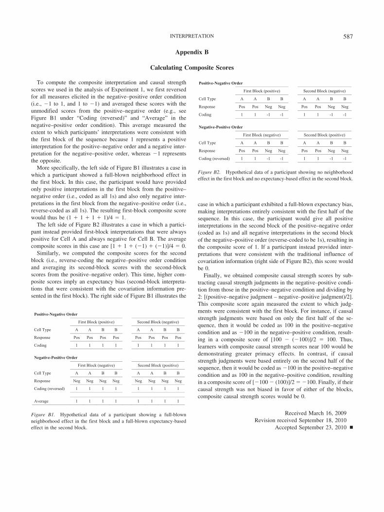
Appendix B

Calculating Composite Scores

To compute the composite interpretation and causal strengthscores we used in the analysis of Experiment 1, we first reversedfor all measures elicited in the negative–positive order condition(i.e., 1 to 1, and 1 to 1) and averaged these scores with theunmodified scores from the positive–negative order (e.g., seeFigure B1 under “Coding (reversed)” and “Average” in thenegative–positive order condition). This average measured theextent to which participants’ interpretations were consistent withthe first block of the sequence because 1 represents a positiveinterpretation for the positive–negative order and a negative inter-pretation for the negative–positive order, whereas 1 representsthe opposite.

More specifically, the left side of Figure B1 illustrates a case inwhich a participant showed a full-blown neighborhood effect inthe first block. In this case, the participant would have providedonly positive interpretations in the first block from the positive–negative order (i.e., coded as all 1s) and also only negative inter-pretations in the first block from the negative–positive order (i.e.,reverse-coded as all 1s). The resulting first-block composite scorewould thus be (1 � 1 � 1 � 1)/4 � 1.

The left side of Figure B2 illustrates a case in which a partici-pant instead provided first-block interpretations that were alwayspositive for Cell A and always negative for Cell B. The averagecomposite scores in this case are [1 � 1 � (1) � (1)]/4 � 0.

Similarly, we computed the composite scores for the secondblock (i.e., reverse-coding the negative–positive order conditionand averaging its second-block scores with the second-blockscores from the positive–negative order). This time, higher com-posite scores imply an expectancy bias (second-block interpreta-tions that were consistent with the covariation information pre-sented in the first block). The right side of Figure B1 illustrates the

case in which a participant exhibited a full-blown expectancy bias,making interpretations entirely consistent with the first half of thesequence. In this case, the participant would give all positiveinterpretations in the second block of the positive–negative order(coded as 1s) and all negative interpretations in the second blockof the negative–positive order (reverse-coded to be 1s), resulting inthe composite score of 1. If a participant instead provided inter-pretations that were consistent with the traditional influence ofcovariation information (right side of Figure B2), this score wouldbe 0.

Finally, we obtained composite causal strength scores by sub-tracting causal strength judgments in the negative–positive condi-tion from those in the positive–negative condition and dividing by2: [(positive–negative judgment – negative–positive judgment)/2].This composite score again measured the extent to which judg-ments were consistent with the first block. For instance, if causalstrength judgments were based on only the first half of the se-quence, then it would be coded as 100 in the positive–negativecondition and as 100 in the negative–positive condition, result-ing in a composite score of [100 (100)]/2 � 100. Thus,learners with composite causal strength scores near 100 would bedemonstrating greater primacy effects. In contrast, if causalstrength judgments were based entirely on the second half of thesequence, then it would be coded as 100 in the positive–negativecondition and as 100 in the negative–positive condition, resultingin a composite score of [100 (100)]/2 � 100. Finally, if theircausal strength was not biased in favor of either of the blocks,composite causal strength scores would be 0.

Received March 16, 2009Revision received September 18, 2010

Accepted September 23, 2010 �

Positive-Negative Order

First Block (positive) Second Block (negative)

Cell Type A A B B A A B B

Response Pos Pos Pos Pos Pos Pos Pos Pos

Coding 1 1 1 1 1 1 1 1

Negative-Positive Order

First Block (negative) Second Block (positive)


Response Neg Neg Neg Neg Neg Neg Neg Neg

Coding (reversed) 1 1 1 1 1 1 1 1

Average 1 1 1 1 1 1 1 1

Figure B1. Hypothetical data of a participant showing a full-blownneighborhood effect in the first block and a full-blown expectancy-basedeffect in the second block.

Positive-Negative Order

First Block (positive) Second Block (negative)


Response Pos Pos Neg Neg Pos Pos Neg Neg

Coding 1 1 -1 -1 1 1 -1 -1

Negative-Positive Order

First Block (negative) Second Block (positive)


Response Pos Pos Neg Neg Pos Pos Neg Neg

Coding (reversed) 1 1 -1 -1 1 1 -1 -1

Figure B2. Hypothetical data of a participant showing no neighborhoodeffect in the first block and no expectancy-based effect in the second block.

587INTERPRETATION

Expectations and Interpretations During Causal Learning · Expectations and Interpretations During...

Documents

Transcript of Expectations and Interpretations During Causal Learning · Expectations and Interpretations During...