Expectations and Exchange Rate Policy

Michael B. Devereux Charles Engel

UBC Wisconsin

April 24, 2006

Abstract

Both empirical evidence and theoretical discussion have long emphasized the impact of `news’ on exchange rates. In most exchange rate models, the exchange rate acts as an asset price, and as such responds to news about future returns on assets. But the exchange rate also plays a role in determining the relative price of non-durable goods when nominal goods prices are sticky. In this paper we argue that these two roles may conflict with one another. If news about future asset returns causes movements in current exchange rates, then when nominal prices are slow to adjust, this may cause changes in current relative goods prices that have no efficiency rationale. In this sense, anticipations of future shocks to fundamentals can cause current exchange rate misalignments. Friedman’s (1953) case for unfettered flexible exchange rates is overturned when exchange rates are asset prices. We outline a series of models in which an optimal policy eliminates the effects of news on exchange rates.

We thank participants in seminars at the European Central Bank and the International Monetary Fund. We thank Joong-Shik Kang for research assistance. Engel received support for this research from a grant from the National Science Foundation, Award No. SES -0451671.

Much of analysis of open economy macroeconomics in the past 30 years has been built on the

foundation that exchange rates are asset prices and that some goods prices adjust more slowly than asset

prices. If this is true, it means that exchange rates wear two hats: They are asset prices that determine the

relative price of two monies, but they also are important in determining the relative prices of goods in

international markets in the short run. For example, if export prices are sticky in the exporting currency,

then nominal exchange rate movements directly change the terms of trade. While of course the literature

has recognized this dual role for exchange rate movements, it has not recognized the implication for

exchange-rate or monetary policy. Asset prices move primarily in response to news that alters

expectations of the future. Most exchange rate movements in the short run reflect changes in expectations

about future monetary or real conditions. But future expectations should not be the primary determinant

of the relative price of nondurable goods. Those relative prices ought to reflect current levels of demand

and supply. So, news that causes nominal exchange rates to jump may have undesirable allocational

effects as the news leads to inefficient changes in the relative prices of goods. It may be that controlling

exchange rates – dampening their response to news – is an important objective for monetary policy.

The “asset market” approach to exchange rates has long recognized that exchange rate

movements are primarily driven by news that changes expectations. For example, the survey of the field

by Frenkel and Mussa (1985, p. 726) in the Handbook of International Economics states: “These facts

suggest that exchange rates should be viewed as prices of durable assets determined in organized markets

(like stock and commodity exchanges) in which current prices reflect the market’s expectation concerning

present and future economic conditions relevant for determining the appropriate values of these durable

assets, and in which price changes are largely unpredictable and reflect primarily new information that

alters expectations concerning these present and future economic conditions.” In their monograph,

Foundations of International Macroeconomics, Obstfeld and Rogoff (1996, p. 529) state “One very

important and quite robust insight is that the nominal exchange rate must be viewed as an asset price.

Like other assets, the exchange rate depends on expectations of future variables.”

At the same time, a broad part of the literature has accepted, as Dornbusch (1976, p. 1161-1162)

puts it, “the fact of differential adjustment speeds in goods and asset markets.” Indeed, it was this

difference in the speed of adjustment that led Milton Friedman (1953, p. 165) to advocate for flexible

exchange rates: “If internal prices were as flexible as exchange rates, it would make little economic

difference whether adjustments were brought about by changes in exchange rates or equivalent changes in

internal prices. But this condition is clearly not fulfilled…At least in the modern world, internal prices

are highly inflexible.”

Friedman’s case for flexible exchange rates was derived, however, in a world in which capital

flows were absent. In his world, the exchange rate would determine the terms of trade, but it was not

forward looking and did not reflect expectations of the future as would an asset price. But when the

exchange rate changes are primarily driven by news, the terms of trade or other international prices may

be badly misaligned in the short run.

The misalignment of relative prices is at the heart of the monetary policy analysis in modern

macroeconomic models of inflation targeting. Woodford (2003, p. 12-13) explains: “when prices are not

constantly adjusted, instability of the general level of prices creates discrepancies between relative prices

owing to the absence of perfect synchronization in the adjustment of the prices of different goods. These

relative-price distortions lead in turn to an inefficient sectoral allocation of resources, even when the

aggregate level of output is correct.”

Here, we are focusing on possibly severe misalignments in relative prices when large changes in

exchange rates are caused by changes in expectations. This distortion would not be present if all goods

prices changed flexibly. Then relative prices would not be forced to incorporate these expectations

effects, and nominal goods prices would react (efficiently) to news about the future.

To help focus the central idea of this paper, it is useful to make a list of things we are not saying:

1. We are not saying that other models of monetary policy in open economies have not modeled

exchange rates as asset prices. They have. Our central insight is that monetary policy must react to news

that moves exchange rates. In existing models, the only news that hits the market is shocks to current

economic variables. By targeting current economic variables in those models, monetary policy does

effectively target the news. But in a realistic model, agents have many other sources of information than

simply shocks to current macro aggregates. Targeting the aggregates does not achieve the goal of

offsetting the influence of news on relative prices. Our model explicitly allows agents to have

information about the future that is different than shocks to the current level of macro variables.

2. We are not looking at differences in the information set of the market and policy makers. While

that may be an interesting area for study, it is not our primary concern. To make this clear, we model the

market and policy makers as having the same information.

3. The problem we have pinpointed is not one of “excess volatility” in asset prices. We do not

construct a model in which there is noise or bubbles in asset prices. Instead, we model the exchange rate

as the no-bubble solution to a forward-looking difference equation, so it is modeled as an efficient,

rational expectations, present discounted value of expected future fundamentals. Indeed, as West (1988)

has demonstrated, the more news the market has, the smaller the variance of innovations in the exchange

rate. Nonetheless, it is the influence of that news on exchange rates that concerns us. Our intuition is that

movements in nominal exchange rates caused by noise or bubbles would also be inefficient, but we

purposely put aside that issue for others to study.

4. We are not saying that monetary policy should target all asset prices, such as equity prices. Our

2

intuition is that exchange rates are different. Exchange rates are the only asset price whose movement

directly causes a change in the relative price of two non-durables that have fixed nominal prices. That

happens because nominal prices of different goods (or the same good sold in different locations) can be

sticky in different currencies. Fluctuations in other asset prices cause a change in the price of a durable

(e.g., equity prices are the price of capital) relative to the price of a non-durable. At least in some

circumstances, that fluctuation is not a concern of monetary policy. As Woodford (2003, p. 13) explains,

“Large movements in frequently adjusted prices – and stock prices are among the most flexible – can

instead be allowed without raising such concerns, and if allowing them to move makes possible greater

stability of the sticky prices, such instability of flexible prices is desirable.”

5. Our concerns about how news influences exchange rates and affects relative goods prices do not

depend on whether internationally traded goods prices are set in the producers’ currencies (PCP) or the

consumers’ currencies (LCP). Some of our earlier work (Devereux and Engel, 2003, 2004) has focused

on that issue, in models where news was not important. But we set aside that dispute here. If there is

PCP, then nominal exchange rate changes (arising from news of the future) can lead to inefficient changes

in the terms of trade. If there is LCP, these nominal exchange rate changes lead to inefficient deviations

from the law of one price.

6. We are not saying that a policy of fixed nominal exchange rates is optimal. First of all, in response to

traditional contemporaneous disturbances (non-news shocks), exchange rate adjustment may be desirable.

But even with news shocks alone, our results do not necessarily say that exchange rates should be fixed,

but that unanticipated movements in exchange rates should be eliminated. In fact, anticipated movements

in exchange rates may play a role in facilitating relative price movements after a news shock. In general,

our point is that news shocks can lead to relative price distortions that are translated through exchange

rate changes, and these shocks should be a target of policy.

Technically, our model is simple. The central idea is based on the property that efficient relative

prices of non-durable goods depend only on current fundamentals, and should not be directly linked to

news about future fundamentals. This property is satisfied in most recent general equilibrium exchange

rate models. In fact, the clearest statement of independence of current allocations on future fundamentals

is in Barro and King (1984). They show that in general equilibrium models with time-additive utility and

absenting investment, current (efficient) equilibrium allocations are independent of expectations about

future fundamentals. This result extends to an open economy where markets are sufficiently complete to

support a time-invariant risk sharing rule. But, in the presence of sticky nominal prices, this dichotomy

between current allocations and future fundamentals no longer necessarily holds. When prices cannot

adjust, any news shocks that affect the current exchange rate automatically affect relative prices. In

general this is inefficient, and the monetary authority should take action to dampen or eliminate the

3

impact of news shocks on current allocations.

Section 1 presents some empirical evidence on the importance of news in moving exchange rates.

Section 2 then explains in a general context why prices of nondurables should not act like asset prices and

reflect expectations of future fundamentals. The rest of the paper demonstrates the logic of targeting

shocks to exchange rates caused by news in two different models. Section 3 describes the first model, in

which prices are pre-set one period in advance, and can fully adjust after one period. In this model, we

find that an optimal monetary policy in face of news shocks is to maintain a fixed exchange rate. Section

4 then extends the model to allow gradual price adjustment. The extended model no longer calls for a

fixed exchange rate, but implies that an optimal monetary rule eliminates the impact of news shocks on

the exchange rate. In section 5, we build a more realistic model with investment. Optimal investment

decisions are forward looking, so in this model it is no longer strictly true that current relative goods

prices should not depend on future productivity shocks. Nonetheless, under standard parameterizations,

our conclusions are not altered – optimal monetary policy should not only target inflation but also try to

eliminate the effect of news on exchange rates.

Section 1. Empirical Evidence on the Effect of Expectations on Exchange-Rate Volatility

Several recent empirical papers have emphasized the role of news in driving exchange rates.

Engel and West (2005) demonstrate that standard exchange rate models do not in fact imply that

exchange rate changes should be predictable using current values of fundamental variables, or even

necessarily strongly correlated with contemporaneous changes in fundamentals. Instead, they show that a

testable hypothesis of the models is that the news that is incorporated in exchange rates should help the

exchange rate forecast future macroeconomic variables. They find empirical evidence to support that

position.

Andersen, et. al. (2003) use six years (1992-1998) of real-time quotations from the foreign

exchange market to assess the impact of macroeconomic news on exchange rates. They measure “news”

as the difference between announced values of macro variables (payroll employment, trade balance, retail

sales, etc.) and a survey measure of the market’s expectation of these announcements. They find that

exchange rates react significantly to these announcements, and over 5-minute windows, a simple OLS

regression of the exchange rate on the news yields high R2 values: “often around 0.3 and sometimes

approaching 0.6.” While the emphasis in Andersen, et. al. is on the short-run influence of news on

exchange rates, Faust, et. al. (2005) use real-time data and information from the term structure of interest

rates to examine how news announcements affect expectations of long-run exchange rate changes. They

find that news announcements about U.S. real or nominal activity move exchange rates and also influence

longer-term interest rates, with the maximum effect at 2 years. They argue that the effect on long-term

4

rates might reflect the response of long-run changes in expected currency depreciation.

Here we provide some alternative evidence on the effect of changes in expectations on exchange

rates. In particular, we consider models in which the exchange rate can be expressed as a present

discounted value of current and future fundamentals:

(1.1) 0

(1 ) ( | )jtI t j t

jx b b E f I

∞

+=

≡ − ∑ , 0 1b< < .

Here, tf measures the economic “fundamentals” that drive the log of the exchange rate. The discount

factor is b. represents the information set of agents. It is helpful to rewrite this as: tI

(1.2) 1

(1 ) ( | )jtI t t j t t

jx f b b E f f

∞

+=

= + − −∑ I .

Our models suggest that monetary policy should have as one objective the stabilization of innovations

(unexpected changes) in the second term on the right-hand-side of equation (1.2). That is, monetary

policy should work to offset the effects of news shocks on exchange rates that work through unexpected

changes in future fundamentals relative to the current fundamental. How important is this second term in driving exchange rate innovations relative to the effect of

innovations in the current fundamental? We would like to know how much of the variance of unexpected

changes in tIx can be attributed to innovations in the current fundamentals, tf . That is, we would like to

calculate

(1.3) 1

1

var( ( | ))var( ( | ))

t t tt

tI tI t

f E f Ix E x I

η −

−

−≡

−.

Our premise is that innovations in current fundamentals do not contribute much to the variance of

innovations in tIx . We believe that it is mostly news about future fundamentals that causes variation in

tIx . If our hypothesis is correct, then tη should be small.

However, it seems hopeless to measure the variances in the numerator and denominator of

equation (1.3), because we do not have the information the market uses in forming its expectations. We

can calculate a measure of the expected discounted sum of current and future fundamentals based on the

information set available to the econometrician, . Define tH

(1.4) 0

(1 ) ( | )jtH t j t

jx b b E f H

∞

+=

= − ∑ .

But as West (1988) shows, we can only construct upper bounds for the variances in equation (1.3). That

is, from West, we have

, and

.

1var( ( | )) var( ( | ))t t t t t tf E f I f E f H−− < − 1−

1 1var( ( | )) var( ( | ))tI tI t tH tH tx E x I x E x H− −− < −

5

Having an upper bound on both the numerator and the denominator does not help us establish even an

upper bound on tη .

We could follow the method of Campbell and Shiller (1987), and impose that the log of the

exchange rate exactly equals tIx . Their methods then allow one to extract the relevant information in

because that information is reflected in exchange rate movements. But as Engel and West (2005) argue,

that approach requires that we have measures of all the relevant fundamentals that drive the exchange

rate. While one might plausibly argue that the fundamentals for some asset prices such as equities are

completely observable ex post (that is, dividends are observable), it is much less plausible to assert that

we can observe all the fundamentals that drive exchange rates, which include such variables as money

demand shocks, productivity shocks, etc. If the fundamentals are not ex post observable, we cannot apply

the procedures of Campbell and Shiller (1987).

tI

We can, however, rely on a result of Engel and West (2004) to get a measure of the denominator

of tη from equation (1.3). They show that as the discount factor gets large ( ), the

econometrician’s measure of the variance of innovations in the present value is approximately equal to

the variance based on the market’s information set:

1b →

. 1 1var( ( | )) var( ( | ))tI tI t tH tH tx E x I x E x H− −− ≈ −

Even though the econometrician cannot replicate the information set of the market, he can accurately

measure the variance of the innovation in the discounted sum when the discount factor is large. Engel

and West show that in practice the discount factors implied by common empirical models are large

enough that the approximation is a good one.

Engel and West (2004) proceed to show that the volatility of innovations in the actual exchange

rate is approximately twice the size of 1var( ( | ))tI tI tx E x H −− for U.S. exchange rates relative to other G7

countries using two familiar models of exchange rates.1 The first is a monetary model, in which the

observed fundamental is measured as * *(t t t t t )f m y m y= − − − , the log of the money/output ratio in the

U.S. relative to another country. The fundamentals in this model correspond approximately to those in

our model in section 3. The second is a model based on a Taylor rule for monetary policy, in which the

fundamental can be written as either *t t tf p p= − , the difference in the log of U.S. versus foreign-country

prices, or * (t t t t t*)f p p i i= − + − , the sum of the log of the price level and the interest rate in the U.S.

relative to another country. Engel and West (2005) demonstrate how these fundamentals are derived from

the underlying model. These fundamentals correspond to the ones in our model in sections 4 and 5. The

1 Engel and West (2004) rely on a result of Engel and West (2005) to show that innovations in the log of the exchange rate can be measured approximately by change in the log of the exchange rate when the discount factor is near one.

6

fact that exchange rate innovations are more volatile than innovations in the discounted sum of current

and expected future fundamentals indicates either that there are “fundamentals” that are not included, or

that exchange rates may be driven by non-fundamental sources.

Our objective here is not to ask whether economic fundamentals from traditional models can

account for exchange rate volatility. Instead, we take the set of observed fundamentals as given, and

simply try to measure tη . Using the Engel-West theorem, we can approximately calculate the variance in

the denominator of equation (1.3). As we have noted, we can calculate an upper bound on the variance in

the numerator, and hence can calculate an upper bound for tη .

Table 1 reports our measure of tη for the fundamentals considered by Engel and West (2004), for

various values of the discount factor, b. In calculating these statistics, we take the econometrician’s

information set to be only current and lagged values of the fundamentals, tf . We estimate an

autoregression with four lags (in all cases) on each measure of the fundamentals. From these, we

calculate our estimates of and 1var( ( | ))t t tf E f H −− 1var( ( | ))tI tI tx E x H −− .

We use the same data used in Engel and West (2004, 2005). It is quarterly data, 1973:1-2003:1.2

The US is the home country, and we measure the fundamentals relative to the other G7 countries. The

money supplies are seasonally adjusted M1 (except for the UK, for which we use M4) from the OECD

Main Economic Indicators. The US money supply data is corrected for “sweeps”, as described in Engel

and West (2004), using data from the Federal Reserve Bank of St. Louis. We use seasonally adjusted

GDP from the same source (except for Germany, which combines data from the IMF’s International

Financial Statistics (IFS) with the OECD data.) The interest rates are 3-month Eurocurrency returns

taken from Datastream. The consumer prices are from the IFS.

While the estimated value of tη varies from country to country, typically we find that it is around

0.20. More precisely, the average across all countries and all measures of the fundamentals, in the case of

is 0.215. The average is slightly higher for lower values of b and lower for higher values of b.

That is, most of the surprise movement in the discounted sum that is supposed to determine exchange

rates comes from innovations in expected future values of fundamentals rather than unexpected changes

in current values.

0.99b =

It is important to note that the upper bounds for tη reported in Table 1 might be crude upper

bounds. That is, innovations in the current fundamentals might contribute much less to innovations in tIx

than the numbers reported in this Table. For example, during 2005, the Federal Reserve raised the Fed

Funds rate by 25 basis points each time that the FOMC met. Fed Funds futures indicated before each

2 In a few cases, the time span differs because of data availability. See Engel and West (2005) for data spans.

7

meeting that there was virtual certainty that the Fed would raise rates. That is, there was essentially no

innovation in the current fundamental – the interest rate – on the FOMC meeting days. But clearly the

Fed’s policy decisions are important for exchange rates, and that is reflected in exchange rate movements

on those FOMC days. The exchange rate, however, was not changing because of any surprise in the

current fundamental. The news that hit the market came in the announcements of the Fed’s assessment of

market conditions, which in turn imparted news about future interest rate changes. Our measure of the

variance in the innovations in the current fundamental, 1var( ( | ))t t tf E f H −− , is a crude one because the

market uses much more information than four quarterly lags of the fundamentals to form its expectations.

For example, our measure does not even use the Fed funds future rates to help capture the market’s

information about future interest rates, and so we tend to overestimate the variance of innovations in

current fundamentals.

Section 2. A General Result

The technical result of the paper rests on an insight into dynamic general equilibrium models first

discussed by Barro and King (1984). In a closed economy model with time-additive utility and without

endogenous investment, they show that all real allocations and relative prices are determined solely by

contemporaneous fundamentals. That is, there are no intrinsic inter-temporal links between periods, and

no persistence in the effects of shocks, apart from that due to persistence in the shocks themselves. An

equilibrium allocation in their model is Pareto efficient, since there is a representative individual and all

prices are fully flexible. It follows that, in an economy with sticky prices, if an optimal monetary policy

is designed to replicate the flexible price equilibrium, it should insulate current allocations and relative

prices against shocks that come in the form of announcements about future fundamentals.

We develop this basic intuition within the standard two-country environment of recent open

economy macroeconomic models. We first set out a general version of the model, to illustrate the logic of

Barro and King within our framework. We then apply this model to two particular types of price setting

environments – one where prices are pre-set one period ahead for just one period, and then to an

environment of Calvo-type staggered pricing. In each case, we identify one or more optimal monetary

policy rules to deal with news shocks.

Although the analytical results rely on the strict separation across periods, we do not argue that it

be taken literally. There are a number of factors that give rise to efficient links between current

allocations or relative prices and future fundamentals shocks. One obvious channel is investment. But

we argue that even once we allow for this linkage, our central result, that the current exchange rate

response to announcements about future fundamentals should be dampened, will still hold in a

quantitative sense. An extension of the model to allow for endogenous investment establishes this point.

8

The Basic Model

Take a general example of an open economy macro model. Say that there are two equally sized

countries: home and foreign, where in each country the measure of households is normalized to one. In

each country, households maximize expected lifetime utility taking prices and wages as given.

Households consume traded goods, constituting a mix of home and foreign goods, and a non-traded good,

produced and consumed only in the domestic country. Firms are monopolistic and maximize utility for

their owners. Say that consumer preferences are:

00

tt

t

E β υ∞

=

ϒ = ∑ , 0 1,β< <

where ( , ) ( / )t t t tU C L V M Ptυ = + , with Here C represents aggregate

consumption, L is labor supply, and

1 2 11 220, 0, 0, 0.U U U U> < < <

/M P are real money balances. Aggregate consumption C is a

function of non-traded consumption and traded consumption; ( , )N TC C C C= . Traded consumption is

also a function of home and foreign traded goods consumption; ( ,T T H FC C C C )= . Each function is

homogenous of degree 1, and each argument of these functions is a homogenous of degree 1 function of a

continuum of differentiated individual goods, with constant elasticity of substitution λ across varieties.

The price index P reflects the weights implied by the consumption aggregator, and

, where again each function is homogenous of degree 1. ( , ) ( , ( , ))N T N T H FP P P P P P P P P= =

Firms are monopolistic competitors, and set prices as a markup over marginal cost. Assume first

that all prices are fully flexible. In addition, let the production technologies of typical firms in the non-

traded and traded sectors of the home country economy be (ignoring firm specific notation):

, .N N HY L Y LHθ θ= =

Thus, there is a common technology shock to both sectors, and the only input to production is labor.

Finally, we assume that there exists a full set of state contingent assets for sharing consumption risk

across countries. There is only one type of fundamental shock in this model, a shock to the country

specific technologies. But the argument may be easily generalized to other shocks. It is straightforward to show that the equilibrium of this economy, where all households within a

country and all firms within a sector are identical, may be represented by the following conditions (letting

foreign variables be denoted with an asterisk).

(2.1) 2

1

( , )1 ( , )

Ht t t

t t

P U CP U C Lt t

Lλλ θ−

=−

,

(2.2) 1( , )Nt Nt Tt tL P P P Cθ = ,

(2.3) * * * * * *1 1 1 1( , ) ( , ) ( , ) ( , ) *

Ht Nt Tt T t Ht Ft t t Nt Tt T t Ht Ft tL P P P P P P C P P P P P P Cθ = + ,

9

(2.4) *

* * *1 1( , ) ( , ) t t

t t t tt

S PU C L U C LP

= Λ .

Equation (2.1) relates the equilibrium real price for home goods to the price-cost markup times the firm’s

marginal cost, represented by the ratio of the real wage to the technology variable. Since non-traded and

traded goods share the same technology, and labor is mobile across sectors, this condition is the same for

both sectors (so that ). Equations (2.2) and (2.3) represent market clearing in the home non-

traded and traded goods markets, respectively, where the notation represents the first

derivative of the price index with respect to the first argument, etc. Finally, equation (2.4) represents the

risk-sharing condition across countries, relating marginal utilities to the real exchange rate (where is

the nominal exchange rate), for a time-invariant constant

Nt HtP P=

1( , )N TP P P

tS

Λ .

Equations (2.1)-(2.3), their analogues for the foreign economy, and equation (2.4) represent a

general equilibrium in seven equations that determine the endogenous variables (where tildes denote

equilibrium values); and * *, , , , ,t t Nt Ht Nt HtC C L L L L* ,*

t Ftt

Ht

S PP

τ = , the terms of trade.

The key feature of this solution is that it represents a mapping from contemporaneous technology

shocks tθ and *tθ to the equilibrium values of endogenous variables. More particularly, future

technology shocks have no impact on allocations or the terms of trade. In fact, the system (2.1)-(2.4)

contains no past or future variables at all (except Λ , which reflects initial wealth based on initial

expectations, and which is not time-varying.) The following result then immediately follows. If nominal

prices and HP *FP are sticky, and the monetary authority follows a rule aimed to sustain the flexible price

equilibrium of the model described by (2.2)-(2.4), then it must necessarily choose a value of the nominal

exchange rate that is independent of unanticipated current announcements about future technology shocks

(or news shocks). If this were not the case, then news shocks would affect the current terms of trade, and

allocations would be pushed away from the flexible price equilibrium of the model.

We now explore the implication of this result in a number of settings where prices are sticky.

Section 3. A Model with One-period Price Setting.

We now apply this result to a model where prices are pre-set for one period. The model is a

simple extension of Devereux and Engel (2003) (henceforth DE) and is based also on Duarte and Obtsfeld

(2005). We let:

1

111 1

tt t

t

MC LP

ε

ρ χtυ η

ρ ε

−

− ⎛ ⎞= + ⎜ ⎟− − ⎝ ⎠

− , 0>ρ , 0>ε ,

10

where 1

(1 )(1 )T NC CCγ γ

γ γγ γ

−

−=−

and . The parameter .5 .52T HC C C= F γ represents the share of traded goods in

consumption. The price indices P are defined by 1T NP P Pγ γ−= , and . 0.5 0.5

T H FP P P=

Following Beaudry and Portier (2003), we assume that technology shocks have a component that

is known one period in advance of the shock. Thus, for the home country, we assume that the technology

shock is

1 2 1 1 2, exp( ), exp(t t t t t t tv u ),θ θ θ θ θ−= = =

where and are normally distributed, with mean zero, and variance tv tu 2vσ and 2

uσ respectively. The

critical feature of the technology process is that the innovation in 1tθ becomes known one period in

advance, i.e. at time t - 1. On the other hand, the component 2tθ , is realized at the same time as it

becomes known.3 The implication of this assumption is that households and firms will know part of

future technology innovations one period in advance. Hence, since in this version of the model prices are

pre-set for only one period, prices for future periods can fully adjust to a forecast in the technology shock.

But prices for the current period, based on period t - 1 information, cannot adjust to the shock. The solution to the model follows closely that of DE. An approximation to the money market

equilibrium may be written as:

(3.1) 1 11 ( )t t t t t t t t tm p c E p E c p ci

ρ ρ ρ mε ε + +− = − + − − + Γ ,

where is a constant, i is the steady-state nominal interest rate, and lower-case letters refer to logs of

the respective variables. An analogous condition may be derived for the foreign country. mΓ

The optimal trade-off between consumption and leisure implies:

(3.2) ηρ =tt

t

CPW

.

The risk sharing condition implies:

(3.3) *

0 *t t t

t t

S P CP C

ρ⎛ ⎞

= Γ ⎜ ⎟⎝ ⎠

,

where depends on initial conditions and is not time-varying. 0Γ

Price Setting

Prices for period t are set one period in advance, based on period t - 1 information sets. Firms

3 Beaudry and Portier (2003) assume that the forecastable component of technology is permanent. Here we assume that it is transitory. This makes little difference to the results of this section. In section 4, some of details of the results are altered in the presence of a permanent forecastable technology shock, although the central result (eliminating surprise exchange rate changes) is unchanged.

11

choose prices to maximize profits using the stochastic discount factor of their owners. We allow for

exported goods prices to be set either in the firm’s own currency (producer currency pricing, or PCP) or

in foreign currency (local currency pricing, or LCP).

Equilibrium

The goods market equilibrium condition in the home country non-traded goods sector is:

(3.4) (1 ) t tt Nt

Nt

PCLP

θ γ= − ,

where represents employment in the non-traded goods sector. In the traded goods sector, for the PCP

pricing environment, the equilibrium condition is ( is employment in the home traded goods sector):

NtL

HtL

(3.5) * *1

2t t t t t

t HtHt Ht

PC S P CLP P

θ γ⎛ ⎞

= +⎜ ⎟⎝ ⎠

.

With LCP the goods-market equilibrium condition in the home traded goods sector is written as:

(3.6) * *

*

12

t t t tt Ht

Ht Ht

PC P CLP P

θ γ⎛ ⎞

= +⎜ ⎟⎝ ⎠

.

The difference between (3.5) and (3.6) is due to the fact that in the latter case there are separate pre-set

prices of home goods in domestic currency (for domestic sales) and foreign currency (for export).

Flexible-Price Solution

With flexible prices, we may apply the conditions (2.1)-(2.4) to solve for consumption and the

terms of trade as:

(3.7) ( )1

11 ( / 2) *( / 2)

1t t tCρ γ γ ρλη θ θ

λ

−−⎛ ⎞= ⎜ ⎟−⎝ ⎠

,

(3.8) 1

10 *

tt

t

γ θτ

θ−= Γ .

Without non-traded goods, consumption would be equalized across countries. Generally

however, with γ < 1, home consumption is more sensitive to a home technology shock than to a foreign

technology shock.

Monetary Policy Rules

Money supply of each country is given by:

(3.9) 1 1t t t tm m µ δ− −= + +

(3.10) * * * *1 1t t t tm m µ δ− −= + + .

Monetary policy rules are designed to respond to unanticipated shocks, so , and

will hold. Here

*1 1( ) ( ) 0t t t tE Eµ µ− −= =

*2 1 2 1( ) ( )t t t tE Eδ δ− − − −= 0= tµ ( *

tµ ) is an addition to the time t information set, while 1tδ −

12

( *1tδ − ) is an addition to the time t - 1 information set. Note that this assumption means that conditionally

(on time t information) expected money growth will vary over time, although the unconditional

expectation of money growth is zero. This monetary rule is designed so that the tµ component reacts to

current shocks, while the tu tδ component reacts to future shocks, which are announced today. tv

Exchange Rate and Consumption under PCP

With PCP pricing, the law of one price holds for traded goods. Hence, from (2.4):

(3.11) * *1 1

(1 )( ) ( ) (t t t t t t t t tc E c c E c s E s1 )γρ− − −

−− = − + − .

Unanticipated changes in the exchange rate will affect the real exchange rate, and therefore relative

consumption levels, to the extent that they alter the international relative price of non-traded goods, which

in this model, is also equal to the terms of trade. Since prices fully adjust after one period, the expected real allocations from next period on will

be governed by (3.7) and (3.8). Therefore:

(3.12) *1 1 1

1 (1 0.5 ) 0.5t t t t t tE c E c v vγ γρ+ − + ⎡ ⎤− = − +⎣ ⎦ .

There are no expected changes in nominal interest rates from time period t + 2 onwards, since the news

shock is then dissipated, and in expectation, the money stock is constant. We can then use this property

and the period t + 1 version of (3.1), to obtain:

(3.13) 1 1 1 1 1 1 1 1

1 1 1 1

( )

(1 ) ( )(1 )

t t t t t t t t t t t t

t t t t t t t t t

1E p E p E m E m E c E c

iE m E m E c E ci

ρε

ρδε

+ − + + − + + − +

− + − +

− = − − −

+= + − − −

+

.

Equations (3.11), (3.12), and (3.13) together with (3.1), and the analogous equations for the foreign

country, lead to the exchange rate:

(3.14)

* ** *

1 11

( 1) (1 )( )(1 ) ( ) ( ) (1 )1 (1 (1 )) 1 (1 (1 ))

t t t tt t t t t t

t t t

i v vi m E m m E m is E si i

ε γ δ δε εγ ε γ ε

− −−

− ⎡ ⎤− − + −⎣ ⎦⎡ ⎤+ − − − +⎣ ⎦− = ++ − − + − −

The exchange rate is the sum of two elements. First, there are revisions to current fundamentals, i.e.

unanticipated movements in relative money growth across the home and foreign country. The second

element is future fundamentals, captured by the second term in (3.14). This is explained as follows.

When , there is a shock to future home productivity that exceeds that to future foreign productivity.

If in addition

*tv v> t

1γ < , this must increase anticipated consumption at home more than in the foreign country,

since home residents’ consumption is more sensitive to home productivity in the presence of a non-traded

goods sector. From (3.1), holding the current monetary innovation constant, a rise in expected future

13

home relative consumption will increase the home nominal interest rate, relative to the foreign nominal

interest rate, when 1ε > . This will reduce demand for money at home relative to the foreign country, and

as a result there is an unanticipated home currency depreciation. Finally, future fundamentals also

incorporate future changes in the relative money supplies, *t tδ δ− , which can be forecasted based on

announcements of future relative technology growth rates.

The key feature of this mechanism is that the exchange rate responds to future fundamentals

rather than current fundamentals. That is, the time t + 1 productivity shock becomes known at time t, and

generates ‘news’, which leads the current exchange rate to move, and the resulting changes in the

expected future money supply have a similar effect. There are no changes in current supply or demand

variables, however.

How do home and foreign consumption rates respond to future productivity shocks? Again from

the money market clearing condition (3.1), we can derive the expression for the unexpected response of

home and foreign consumption, respectively, as:

(3.15) ( )1 1 1 1 1 11 ( 1)( ) ( )

2 (1 ) (1 )t

t t t t t t t t t t t t tic E c m E m s E s E c E c

i iδγ εφ

ε ρ− − − + − +

⎛ ⎞−⎡ ⎤− = − − − + − +⎜ ⎟⎢ ⎥ + +⎣ ⎦ ⎝ ⎠,

(3.16) ( )*

* * * * * *1 1 1 1 1 1

1 ( 1)( ) ( )2 (1 ) (1 )

tt t t t t t t t t t t t t

ic E c m E m s E s E c E ci i

δγ εφε ρ− − − + − +

⎛ ⎞−⎡ ⎤− = − + − + − +⎜ ⎟⎢ ⎥ + +⎣ ⎦ ⎝ ⎠

where 1 11

iiεφ

ρ+⎛ ⎞≡ ⎜ ⎟+⎝ ⎠

.

We may explain these expressions as follows. Take equation (3.15), and imagine that there is an

anticipated positive home country productivity shock. Then there is a rise in expected future home

consumption, which will tend to raise nominal interest rates when 1ε > . This causes an excess supply of

home money, and would lead to an unanticipated rise in current home consumption. Against this,

however, is the fact that the anticipated home productivity shock causes an exchange rate depreciation,

when 1ε > . This reduces real money supply, and tends to reduce home consumption. The net effect on

current period home consumption may be positive or negative. When 1ε < the reasoning goes the other

way.

The impact of future money supply changes are straightforward – a positive tδ represents an

expected future monetary expansion, which raises nominal interest rates and raises current consumption.

Local-Currency Pricing (LCP)

Under local-currency pricing, the law of one price will not generally hold. Since with LCP all

domestic and foreign nominal goods prices are pre-determined, the CPIs of each country are also

14

predetermined. Then, from (3.3), we get:

(3.17) * *1 1

1( ) ( ) (t t t t t t t t tc E c c E c s E sρ− −− = − + − 1 )− .

The behavior of expected period t + 1 consumption is the same as in (3.7), since LCP and PCP are

equivalent to one another after prices have fully adjusted. For the same reason, equation (3.13) is the

same as before. Then, equations (3.17), (3.7), (3.13), and the money market equilibrium conditions (3.1)

for each country, give:

(3.18) * * *1 1 1

1 1 ( 1)( ) ( ) (1 )( )1 (1 ) (1 )t t t t t t t t t t t t t

i is E s m E m m E m v vi i iε ε *γ δ δ

ε− − −

⎛ ⎞+ −⎛ ⎞ ⎡ ⎤ ⎡− = − − − + − − + −⎜ ⎟⎜ ⎟ ⎣ ⎦ ⎣+ + +⎝ ⎠ ⎝ ⎠⎤⎦ .

This differs from expression (3.14) due to the fact that price levels are predetermined under LCP. But

qualitatively, we get a similar message. The exchange rate is a function of current and future

fundamentals. A future productivity shock, which becomes known today, represents `news’, which

impacts on the current exchange rate. The size of this effect depends on the size of the non-traded goods

sector, as well as the size of ε .

The impact of future productivity shocks on consumption is given by:

(3.19) ( )1 1 1 1 11 ( 1)( )

(1 ) (1 )t

t t t t t t t t t tic E c m E m E c E c

i iδεφ

ε ρ− − + − +

⎛ ⎞−− = − + − +⎜ ⎟+ +⎝ ⎠

,

(3.20) ( )*

* * * * * *1 1 1 1 1

1 ( 1)( )(1 ) (1 )

tt t t t t t t t t t

ic E c m E m E c E ci i

δεφε ρ− − + − +

⎛ ⎞−− = − + − +⎜ ⎟+ +⎝ ⎠

These effects are equivalent to the PCP case, save for the absence of the exchange rate from (3.19) and

(3.20), since movements in the exchange rate no longer directly impact on CPI values. But again, as in

the PCP case, we have announcements effects of future productivity shocks influencing current

consumption. This case also allows us to be more precise regarding the impact of future productivity

shocks. Whenever 1ε > , a rise in future home or foreign productivity will lead to a rise in current

consumption. This happens because there is no secondary channel of the initial interest rate increase

arising from the future productivity shock, as exists in the PCP case.

Optimal Monetary Policy with News Shocks

So far we have not been specific about the monetary policy response to current or anticipated

future productivity shocks. Implicit in the analysis above is that current productivity shocks (i.e. shocks

to 2tθ ) have no impact on either the exchange rate or consumption, independent of the endogenous

response of monetary policy. But, following the analysis of DE, there are clear welfare reasons why

monetary policy should be designed to ensure the efficient response of the real economy to current

15

productivity shocks in the presence of sticky prices. The optimal values for the monetary policy response

to current productivity shocks are similar to those analyzed in DE and Duarte and Obstfeld (2005). For

the PCP model, the monetary policy responses in the home and foreign currency can perfectly replicate

the flexible price equilibrium. For the LCP model, given the absence of exchange rate pass-through, the

flexible price equilibrium cannot be sustained. The optimal monetary policy response ensures that

consumption responds to current productivity shocks as in the flexible price equilibrium, but the exchange

rate responds by less than in the flexible price equilibrium.

In face of anticipated future productivity shocks however, the rationale for an optimal policy

response becomes less clear. When there is a shock to 1 1tθ + , which by assumption is observed at time t,

then prices have the chance to respond fully before the shock takes effect. In that case, there is no reason

for monetary policy to be used in order to ensure the efficient adjustment of the period t + 1 allocations to

the productivity shock. But the key feature of our examples above, and the central message of the paper,

is that these anticipated future shocks will affect the economy in the present. That is, by impacting on

interest rates and exchange rates, current consumption will be moved away from its flexible price

equilibrium, given by (3.7). The reason is that, while future prices have time to adjust to the shock that

occurs in period t + 1, current prices cannot react to the announcement. To the extent that the

announcement effects shift current allocations away from their flexible price equilibrium, they are

undesirable, and an optimal monetary policy can be devised to deal with this.

The nature of the optimal monetary policy for future productivity shocks turns out to be the same,

for both types of pricing. Thus, we can state:

Result 1:

Let the monetary policy rules be defined as

. *0 1t ta v a vδ = + t

*t

* * *0 1t ta v a vδ = +

Then for both LCP and PCP, the optimal monetary rule is described by

*0 1

( 1) (1 )(1 ) 2

ia ai

ε γε

−= = − −

+ *

1 0( 1)(1 ) 2

ia ai

ε γε

−= = −

+.

Proof:

These rules eliminate the impact of future productivity shocks on current consumption in both countries.

Therefore, employment is also unchanged. Therefore the rules sustain the flexible price equilibrium, in

face of announced future productivity shocks.

Result 2:

The optimal monetary rules from Result 1 prevent the exchange rate from responding to future

productivity shocks.

Proof: By inspection.

16

Result 2 is in a sense the more interesting one. Standard Optimal Currency Area (OCA)

reasoning suggests that it is efficient to allow the exchange rate to respond to country specific

productivity shocks. We find, in the absence of a monetary response, that indeed the exchange rate will

respond to announcements of country specific productivity shocks. The direction of movement depends

on the size of ε . For 1ε > , the exchange rate will depreciate in response to an announced future home

productivity expansion. It is tempting to interpret this movement along efficiency (or OCA) lines – the

future home productivity expansion should cause a home country terms of trade deterioration. Hence, the

response of agents in financial markets, forecasting this, leads to an immediate nominal exchange rate

depreciation.

But the problem with this reasoning is that the immediate response of the current nominal

exchange rate causes a change in the current real exchange rate (by different degrees in the PCP and LCP

environments), because current nominal prices cannot respond to the announced future shock. In the

absence of a current (as opposed to future) productivity shock, however, there is no efficiency reason for

the real exchange rate to move at all. In fact, movements in the real exchange rate are associated with

welfare losses since they push consumption and employment away from their efficient levels.

Thus, in a sticky price environment, when the exchange rate responds to `news’, there is no

guarantee that it will do so in an efficient manner. Indeed, in our model, the optimal monetary rule should

prevent the exchange rate from responding to news shocks at all. The critical requirement is that there not

be any unanticipated movements in the exchange rate. That is, the time t exchange rate will be known in

time t - 1. Given the form of the monetary rules defined here, we can actually go beyond this, and

establish that under these rules the exchange rate is fixed over time (when all shocks are observed in

advance). To see this, note that

* * *1 1 1 1 1 1 1 1

* * *

* *

( 1)( ) ( )(1 )

( 1) ( 1) (1 )( ) ( )(1 ) (1 )( 1) ( )

(1 )

t t t t t t t t

t t t t t t t t

t t t t t

i *1

*

ts c c p p c c m mi

i ic c m m v vi i

i c c m m si

ρ ερε

ρ ε ε γ δ δε ε

ρ εε

+ + + + + + + +

−= − + − = − + −

+− − −

= − + − + − + −+ +

−= − + − =

+

+

The first equality comes directly from the risk sharing condition (2.5). The second comes from the

solutions for period t + 1 prices discussed before equation (3.13). The third equality comes from a

decomposition of money growth and consumption growth, while the fourth uses the optimal money rule

of Result 1.

Hence, the monetary authority follows a rule in which next period’s money supply responds to

future productivity shocks, letting nominal price levels take the full burden of adjusting the future real

exchange rate to the productivity shocks, and keeping the exchange rate fixed over time. From a welfare

17

perspective however, this is not necessary. The efficient allocation could just as easily be attained by a

policy which prevents the current exchange rate from reacting to news shocks, but allowing part of the

real exchange rate adjustment to occur via movements in the future nominal exchange rate. Thus, there

could be expected changes in the exchange rate over time. These changes would not be costly, because

prices can adjust over the same time frame. The critical ingredient in the analysis is that future

productivity shocks do not generate surprise movements in the current nominal exchange rate.

Of course the model is quite stylized, since we have assumed that all prices can adjust before the

news takes effect. But this is not necessarily unrealistic. At an anecdotal level, we see the exchange rate

responding to all types of potential events (e.g. effects of Social Security changes that may affect the

budget deficit in 5 or more years’ time) that may occur much further in the future than would be relevant

for business cycle frequencies. These exchange rate movements are not necessarily desirable, because we

have to recognize that the response to future shocks may not be consistent with the currently desired

structure of relative prices. Nevertheless, we now turn to an extended version of the model, which

assumes that nominal prices must be adjusted gradually rather than all at once.

Section 4. Extension to Gradual Price Adjustment

We now extend the model to allow gradual price adjustment using the Calvo specification where

only a given fraction of firms may adjust their prices within a period, and ex ante, all firms have an equal

chance of price adjustment. The specification for households and firms is unchanged except for the price

setting rule. For simplicity, we focus only on the PCP pricing case. In addition, to make the analysis

comparable to the previous model, we follow Rotemberg and Woodford (1997) in assuming that a firm

that has an opportunity to change its price must set its price for period t with information based on period

t - 1. That is, prices that are adjusted are set one period in advance, as in the previous model. Unlike the

previous model however, not all prices are adjusted in every period.

Assume that all firms in both countries have a probability1 κ− of receiving an opportunity to

change their price in any period. Then the newly set price for any home country firm in the non-traded

goods sector that can change its price for period t is given by

(4.1) 1

0

10

( )

1 ( )

i t i t it Nt i N

i t i t iNt

i t it Nt i Nt i

i t i

W CE P YPP

CE P YP

t i

ρλ

ρλ

βκθλ

λ βκ

−∞+ +

− += + +

−∞+

− + += +

=−

∑

∑

+

1

.

Using standard properties of the Calvo price setting scheme, we may write the non-traded goods price

index as

(4.2) 1 11 (1 )Nt Nt NtP P Pλ λ λκ κ− −

−= + − − .

18

Now, taking a linear approximation of (4.1) and (4.2) around a zero-inflation steady state, and putting the

two conditions together, we may obtain the conventional forward looking inflation equation, given by

(4.3) 1 1( )Nt t t Nt t t t NtE w p u v E 1 1π ϕ β− −= − − − + π− + .

Since the marginal cost facing firms in the home country traded goods sector is identical to that of the

non-traded goods firm, to a linear approximation the price inflation equation for traded goods will be

identical to (4.3). We then follow the convention of referring to inflation in the home goods price (either

traded or non-traded) as tπ .

To conform to the standard in the literature, we assume now that the monetary authorities follow

an interest rate rule rather than a rule for the money supply. The gross nominal interest rate in the home

economy may be read off the Euler equation as:

(4.4) 1

1

1 t tt t

t t

C CR EP P

ρ ρ

β

− −+

+

⎛ ⎞ ⎛= ⎜ ⎟ ⎜

⎝ ⎠ ⎝

⎞⎟⎠

Again, taking a linear approximation around a steady state:

(4.5) 1 1 1( ) (2t t t t t t t tr r E c c E Eγ )tρ π τ+ + += + − + + −τ

ht

,

where is the home country terms of trade. Assume that the monetary authority follows

an interest rate rule given by:

*t ft tp s pτ = + −

(4.6) t tr r tσπ δ= + + ,

where 1 0t tE δ− = .4 Different assumptions regarding tδ will be examined below. Table 2 describes the

full model.

For simplicity, we deal for now only with the case where all shocks are `news shocks’, so that

.0tu = 5 Note that the flexible price solution to the model is identical to (3.7) and (3.8) above, so that

* * *1 1 1

1 1(1 ) , (1 )2 2 2 2t t t t tc v v c vγ γ γ γ

ρ ρ− − − −⎡ ⎤ ⎡ ⎤= − + = − +⎢ ⎥ ⎢ ⎥⎣ ⎦ ⎣ ⎦

1tv 1, and *1t t tv vτ − −= − . Efficient consumption and

the terms of trade are independent of anticipated future productivity shocks.

The objective of monetary policy, as in the previous section, should be to replicate the response

of the flexible price economy. But in contrast to the previous section, there is an independent welfare cost

of inflation, even if it is perfectly anticipated. This is because in an environment of gradual price

adjustment, inflation generates price dispersion, since not all firms may change their prices

4 Under the Taylor rule given by equation (4.3), inflation is anticipated one period in advance. So targeting actual inflation or one-period ahead anticipated inflation is equivalent. Svensson and Woodford (2005) have advocated inflation forecast targeting. 5 Since the inflation rate is predetermined, an optimal policy response to a current productivity disturbance will require an interest rate adjustment: tδ will need to fall in response to a positive shock. tu

19

simultaneously. By setting inflation to zero, firms will never wish to adjust their prices, and thus price

dispersion will be eliminated. As in Woodford (2003), an optimal monetary policy should therefore

replicate the response of the flexible price economy, while achieving a zero rate of price change.

Table 2

The model with gradual price adjustment

Home inflation 1 1( )

2t t t t t t tE c u v Eγ1 1tπ ϕ ρ τ β π− − −= + − − + +

Foreign inflation * * * *1 1( )

2t t t t t t tE c u v Eγ *1 1tπ ϕ ρ τ β π− − −= − − − + +

Risk sharing *( ) (1t tc c ) tρ γ τ− = −

Home interest rate 1 1 1( ) (

2t t t t t t t t tE c c E Eγ )tσπ δ ρ π τ τ+ + ++ = − + + −

Foreign interest rate * * * * *

1 1 1( ) (2t t t t t t t t t tE c c E Eγ )σπ δ ρ π τ τ+ + ++ = − + − −

Note that so long as the monetary authority follows a rule in which 1σ > , the system in Table 2

is saddle path stable, and there is a unique solution for bounded shock processes.

Case 1. Simple Inflation Targeting

Assume that the monetary authorities follow a simple inflation targeting policy, setting 1σ > , but

not adjusting interest rates to ex-post information, so that 0tδ = . We may write the general solutions for

the terms of trade as . Note that, since all prices are pre-set, the

unanticipated component of the terms of trade;

* * * *0 1 0 1 1 1t t t ta v a v a v a vτ − −= + + + t

t* *

1 1 1t t t tE a v a vτ τ−− = + , is equivalent to the movement in

the nominal exchange rate.

It is easy to verify that:

(4.7) * *0 0 1 1

( 1),1 1

a a a aσϕ σ ϕσϕ σϕ

−= − = = − =

+ +.

The solution for home country inflation is written as:

(4.8) 11t tvϕπσϕ −= −

+.

The consumption responses may be written as:

20

(4.9) * *1 1 t

( -1)1- 1-( +1) 2 2 ( +1) 2 2t t tc v vϕσ γ γ ϕ σ γ γσϕ ρ σϕ ρ− −

⎡ ⎤ ⎡⎛ ⎞ ⎛ ⎞= + +⎜ ⎟ ⎜ ⎟⎢ ⎥ ⎢⎝ ⎠ ⎝ ⎠⎣ ⎦ ⎣tv v ⎤

+ ⎥⎦

,

(4.10) * *1 1

( -1)1- 1-( +1) 2 2 ( +1) 2 2t t tc v vϕσ γ γ ϕ σ γ γσϕ ρ σϕ ρ− −

⎡ ⎤ ⎡⎛ ⎞ ⎛ ⎞= + +⎜ ⎟ ⎜ ⎟⎢ ⎥ ⎢⎝ ⎠ ⎝ ⎠⎣ ⎦ ⎣*t tv v ⎤

+ ⎥⎦

As we increase the `tightness’ of the monetary policy rule (i.e. setting σ → ∞ ), the variance of inflation

falls to zero. This also ensures that the anticipated component of the terms of trade and consumption

responds as in the flexible price equilibrium. But this fails to support the full flexible price equilibrium,

because it does not generate the appropriate response of the terms of trade to contemporaneous news

shocks. In fact, a tight money rule exacerbates the inefficiency of news shocks. As σ increases, the

response of the nominal exchange rate movement to news shocks is increased, generating a larger

(inefficient) terms of trade and consumption movement.6

The intuitive explanation for the relationship between the stance of monetary policy (as described

by the parameter σ ) and the response to news shocks can be understood as follows. Since a positive

news shock will raise future consumption, it will tend to raise real interest rates in both countries. But

with advance price setting and the interest rate rule (4.6), the nominal interest rate is pre-determined with

respect to current news shocks. Moreover, the higher is σ , the smaller is the impact of news shocks on

anticipated inflation. Given that both the nominal interest rate and anticipated inflation are smoothed, the

upshot is that the equilibrium real interest rate is prevented from responding the news shock, and more so,

the higher is σ . This makes the news shock more expansionary in the current period, raising

consumption in both countries.

A similar explanation lies behind the terms of trade response to the news shock. Combining the

two interest rate equations in Table 2, we have an equation in the terms of trade and inflation differentials,

given by:

(4.11) 1 1t t t t t tE Eσ π τ τ π+ +∆ = − + ∆ ,

where *t t tπ π π∆ ≡ − . Again, a news shock will tend to increase the anticipated future terms of trade, as it

increases home relative to foreign productivity. With perfectly flexible prices, the impact would be offset

by a fall in anticipated future relative inflation. But when inflation targeting stabilizes expected inflation,

the change in the anticipated future terms of trade spills over into the current terms of trade.

6 There is no separate role in the Taylor rule for the “output gap.” But, as in Clarida, Gali, and Gertler (2002), we can introduce mark-up shocks that lead output to deviate from efficient levels. When that shock has a common element across countries, the output gap (at home and in the foreign country) should enter the Taylor rule. But even with the output gap in the Taylor rule to deal with this distortion, there remains the distortion when the terms of trade react to news. Terms of trade shocks must enter as a separate term, as in Case 3 below.

21

Case 2. Targeting news shocks.

Now extend the interest rate rule so that 0 1 1t tc v c vtδ −= + for the home authorities, and

for the foreign monetary authorities. Setting * *0 1 1t tc v c vδ −= + *

t 0 1c = − and jointly ensures that

inflation is zero (for any value of

1 1c =

1σ > ) and the terms of trade (and consumption) respond as in the fully

flexible price equilibrium. Note that this implies that the nominal exchange rate is insulated against news

shocks. But it does not mean that the exchange rate is fixed over time. The efficient monetary rule

ensures that the inflation rate of domestic goods prices is zero in each country. Hence all terms of trade

movement must involve exchange rate changes. But the key feature of this rule is that it eliminates any

unanticipated exchange rate changes. The exchange rate will change in response to contemporaneous

productivity shocks. But this change is anticipated one period in advance.

Case 3. Targeting exchange rates.

Since the optimal monetary policy eliminates exchange rate surprises, is there a case for

including the exchange rate directly in the interest rate rule? Say now that the state-contingent component

of interest rate rules for the home and foreign country are given by

(4.12) *1 1( ), (

2 2t t t t t t t tE Eω ω )δ τ τ δ τ τ− −= − = − − .

We may solve the model under this specification. The solution for the terms of trade is given by:

(4.13) * *1 1

1 ( 1)( ) (1 1 1t t t tv v v vσϕ σ ϕτ

σϕ ω σϕ− −−

= − ++ + +

)t− .

This differs from case 1 only due to the presence of the ω expression. But this difference is crucial, for it

allows the policy maker to jointly ensure that the terms of trade responds appropriately to

contemporaneous productivity shocks through an ex-ante `tight money rule’ (i.e. setting σ very high)

raising interest rates in response to anticipated inflation shocks, while at the same time eliminating the

effects of news shocks on the terms of trade through an ex-post interest rate rule which raises interest

rates in response to an unanticipated nominal exchange rate depreciation (setting ω very high). Hence, in

the presence of news shocks, the standard inflation targeting prescription for an optimal monetary rule is

not adequate. It can be improved by an explicit inclusion of the exchange rate in the interest rate rule.

More precisely, the policy-maker should target a low expected rate of inflation, and dampen any

unexpected movements in the nominal exchange rate.

Of course, this analysis pertains only to the response to news shocks. As pointed out in footnote

3 above, to the extent that there are unanticipated current productivity shocks, the optimal monetary

policy should allow the exchange rate to respond immediately. Then, the extent to which monetary policy

22

should accommodate surprise movements in the exchange rate depends on the importance of news shocks

in total exchange rate variability. The empirical evidence in section 1 above, however, suggests that most

of the variance in exchange rate changes that can be attributed to fundamentals is accounted for by non-

contemporaneous movements in fundamentals.

Section 5. Extension to a Model with Investment.

In the models we have analyzed up until now, efficient relative prices (and all other real

allocations) are independent of future productivity realizations. This serves to highlight the inefficiency

generated by having exchange rates change in response to announcements about future productivity

shocks. But it might be argued that a more realistic economic model would allow for intertemporal

linkages between periods. A natural way to do this is by introducing capital into the production process

and exploring the role of physical investment in linking relative prices and allocations between periods.

We now extend the model to allow for physical investment, and in particular we allow current investment

to respond to news shocks about future productivity. We show however that under a conventional

calibration of the model, the results described above hold effectively without any change at all.

Amending the model to allow for investment requires only a few alterations. See the Appendix

for a complete description of the model and its solution. We assume that investment within each country

is defined by an aggregator over non-traded and traded home and foreign goods using the same weights as

the consumption aggregator. Each sector has specific capital which is immobile within a period, but may

be augmented by investment, over time. Thus, defining and as capital of firm i in the

home traded goods and non-traded goods sectors, respectively, and assuming capital is held as an asset by

national residents, we model the evolution of the aggregate capital stock in the standard way as:

( )HtK i ( )NtK i

(5.1) 1 (1 )NtNt Nt Nt

Nt

IK KK

φ δ+

⎛ ⎞= + −⎜ ⎟

⎝ ⎠K ,

(5.2) 1 (1 )HtHt Ht

Ht

IK KK

φ δ+

⎛ ⎞= + −⎜ ⎟

⎝ ⎠HtK ,

where, in each case, we assume that ( ) ( ) ( )' . 0, '' . 0, .φ φ φ δ> < = δ Production functions for the two

sectors are defined as:

(5.3) . 1 1( ) ( ) ( ), ( ) ( ) ( )Ht t Ht Ht Nt t Nt NtY i K i L i Y i K i L iα α α αθ θ− −= =

Again, the productivity shock is assumed to affect both sectors equally.

The previous optimization conditions for the household and firms are augmented in that a)

households choose how much capital to hold, and b) firms’ marginal cost functions now depend on the

rental rate for capital. As before, we explore the impact of a news shock in the same form as above; i.e. a

23

productivity expansion which is announced one period ahead. In this case, we assume that

, where 1 1 1 1exp( )t t tvµθ θ −= − 0 1µ< < .

Figures 1 to 4 illustrate the impact on a news shock in the home country on the terms of trade,

aggregate home consumption, employment and investment under alternative monetary policy rules.

Unlike the previous sections, even in the flexible price equilibrium a news shock impacts upon

contemporaneous allocations through affecting optimal investment. The positive future productivity

shock raises the return on investment today. But at the same time, the rise in future consumption arising

from the future productivity increase raises the current real interest rate. This tends to depress investment

today. The first locus in the Figures illustrates that, if prices are fully flexible, these two forces tend to

offset each other almost exactly. Investment and employment fall very slightly, but consumption and the

terms of trade are effectively unchanged. This indicates that the central requirement of the previous

model – that the efficient level of the current relative prices should be insulated against news shock,

carries over to the extended model with investment, in a quantitative sense.

Figures 1-4 also show the response of the terms of trade, consumption, employment and

investment when prices are sticky (and set according to PCP), under different monetary rules. First, we

look at inflation targeting as in (4.6), assuming that 1.5σ = . In this case, there is a noticeable difference

both in the contemporaneous and the subsequent response to a news shock relative to that of the flexible

price equilibrium. With sticky prices, the news shock has only a small impact on future output and

consumption. This is because, absent a direct monetary policy response, the productivity increase can

only affect output to the extent that prices adjust, and in this model, prices cannot adjust enough within

one period to facilitate an efficient response to the productivity shock. This implies that the real interest

rate increase is considerably less in the initial period. Consumption and investment therefore increase

immediately. Likewise, the terms of trade increases immediately, but the terms of trade increase in the

period in which the shock occurs is less than that in the flexible price equilibrium.

Under strict inflation targeting (i.e. setting σ very high), the results are very much as before.

Strict inflation targeting ensures that the economy responds efficiently to the productivity shock in the

period in which it occurs. Intuitively, when the news shock pertaining to productivity in period t + 1 is

announced, there is a tendency for inflation for period t + 1 to fall, as adjusting firms will revise their

period t + 1 prices downwards. This generates a large downward response in the nominal interest rate for

period t + 1, facilitating an efficient (flexible price equilibrium) response to the shock during period t + 1.

But strict inflation targeting again magnifies the immediate (time t) response of the terms of trade,

consumption, and home country output to a home news shock, as in the previous section.

Finally, the Figures illustrate the effect of allowing interest rates to respond to unanticipated

exchange rate changes in addition to anticipated inflation. That is, we allow a direct response of the

24

interest rate rule to the surprise change in the exchange rate. As before, this policy effectively replicates

the response of the flexible price equilibrium to news shocks. Again, it is efficient to prevent the current

terms of trade from responding to news shocks, and this is done by eliminating unanticipated movements

in the exchange rate.

In summary, this section illustrates that our results are not dependent on the properties of the

simple model of earlier sections, that efficient allocations and relative prices are functions of

contemporaneous productivity shocks alone. Even with an efficient response of investment to anticipated

future shocks, both the results and the policy conclusions carry over essentially unchanged.

Section 6. Conclusions

The examples in the two models of the paper all imply that the exchange rate should be insulated

against the impact of shocks to expectations over future productivity. This is because, with sticky

nominal goods prices, exchange rate movements affect relative prices, and in the models we analyze,

efficient relative prices are independent of future productivity. Even when we allow for efficient

contemporaneous response of investment to news shocks, our numerical results indicate that

unanticipated exchange rate movements generated by news shocks should be eliminated.

The model as formulated makes an assumption of complete markets. When market are

incomplete, news shocks may generate wealth effects that alter current relative prices, even when all

nominal prices are fully flexible. This makes the optimal policy response to news shocks less clear. But

it is still not self-evident that under a policy that ignores news shocks, the exchange rate will move in a

manner consistent with efficient adjustment. More generally, an optimal cooperative monetary policy

may wish to eliminate these wealth effects in any case, and this would be likely to involve dampening the

exchange rate impacts of news shocks.

Our key insight is that consideration of the asset-market approach to exchange rates overturns

Friedman’s (1953) case for unfettered floating exchange rates. Friedman argues that flexible exchange

rates can lead to efficient changes in relative prices when nominal prices adjust sluggishly, but his

framework is one in which exchange rates are not asset prices. When capital is mobile, exchange rate

movements do not effectively substitute for price changes. Experience with floating exchange rates has

shown us that expectations can lead to large and prolonged swings in exchange rates that do not

correspond to any current changes in tastes or technology. Indeed, asset markets may be correctly pricing

the effects of future changes in fundamentals, but the resulting allocations still are not efficient.

Exchange rates cannot simultaneously achieve the asset market equilibrium that reflects news about the

future relative values of currencies and the goods market equilibrium that reflects efficient relative prices.

25

References

Andersen, Torben G.; Tim Bollersev; Francis X. Diebold; and, Clara Vega. 2003. “Micro Effects of

Macro Announcements: Real-Time Price Discovery in Foreign Exchange,” American Economic

Review, 93:1, 38-62.

Barro, Robert and Robert G. King. 1984. “Time-Separable Preference and Intertemporal-Substitution

Models of Business Cycles,” Quarterly Journal of Economics, 99:4, 817-839.

Beaudry, Paul and Franck Portier. 2003. “Stock Prices, News, and Economic Fluctuations,” National

Bureau of Economic Research, working paper no. 10548.

Campbell, John Y., and Robert J. Shiller. 1987. “Cointegration and Tests of Present Value Models,”

Journal of Political Economy 95:5, 1062-1087.

Clarida, Richard; Jordi Gali; and Mark Gertler. 2002. “A Simple Framework for International Monetary

Policy Analysis,” Journal of Monetary Economics 49:5, 879-904.

Devereux, Michael B. and Charles Engel. 2003. “Monetary Policy in the Open Economy Revisited:

Price Setting and Exchange Rate Flexibility,” Review of Economic Studies, 70:4, 765-783.

Duarte, Margarida, and Maurice Obstfeld. 2004. “Monetary Policy in the Open Economy Revisited: The

Case for Exchange-Rate Flexibility Restored,” University of California, Berkeley, manuscript.

Dornbusch, Rudiger. 1976. “Expectations and Exchange Rate Dynamics,” Journal of Political Economy,

84:6, 1161-76.

Engel, Charles, and Kenneth D. West. 2004. “Accounting for Exchange Rate Variability in Present Value

Models When the Discount Factor Is Near One,” American Economic Review, 94:2, 119-125.

Engel, Charles, and Kenneth D. West. 2005. “Exchange Rates and Fundamentals,” Journal of Political

Economy, 113:3, 485-517.

Faust, Jon; John H. Rogers; Shing-Yi B. Wang; and, Jonathan H. Wright. 2005. “The High Frequency

Response of Exchange Rates and Interest Rates to Macroeconomic Announcements,” Journal of

Monetary Economics, forthcoming.

Frenkel, Jacob and Michael Mussa. 1985. “Assets Markets, Exchange Rates, and the Balance of

Payments,” in R. W. Jones and P. B. Kenen, eds, Handbook of International Economics,

(Amsterdam: North Holland).

Friedman, Milton, 1953, “The Case for Flexible Exchange Rates,” in Essays in Positive Economics

(Chicago: University of Chicago Press), 157-203.

Obstfeld, Maurice and Kenneth Rogoff. 1996. Foundations of Open Economy Macroeconomics,

(Cambridge: MIT Press).

26

Obstfeld, Maurice, and Kenneth Rogoff. 2002. “Risk and Exchange Rates.” In Contemporary Economic

Policy: Essays in Honor of Assaf Razin, edited by Elhanan Helpman and Effraim Sadka

(Cambridge: Cambridge University Press).

Rotemberg, Julio and Michael Woodford. 1997. “An Optimization Based Econometric Framework for the

Evaluation of Monetary Policy,” NBER Macroeconomics Annual 1997, 297-346.

Svensson, Lars E. O., and Michael Woodford. 2005. “Implementing Optimal Policy through Inflation-

Forecast Targeting,” in Bernanke, Ben S., and Michael Woodford, eds. (2005), The Inflation-

Targeting Debate, University of Chicago Press, 19-83.

West, Kenneth. 1988. “Dividend Innovations and Stock Price Volatility,” Econometrica, 56:1, 37-61.

Woodford, Michael. 2003. Interest and Prices: Foundations of a Theory of Monetary Policy, (Princeton:

Princeton University Press).

27

Table 1

Upper Bounds for tη from Equation (1.3)

msw-y p i+p

Country b η η η

0.9 0.780 0.258 0.3520.95 0.755 0.225 0.3150.99 0.735 0.200 0.287

1 0.730 0.194 0.280

0.9 0.516 0.117 0.2680.95 0.449 0.067 0.1880.99 0.394 0.034 0.130

1 0.380 0.027 0.116

0.9 0.460 0.184 0.2890.95 0.394 0.119 0.2190.99 0.339 0.072 0.165

1 0.325 0.062 0.151

0.9 0.422 0.130 0.1940.95 0.369 0.078 0.1230.99 0.327 0.042 0.074

1 0.316 0.035 0.063

0.9 0.361 0.243 0.6240.95 0.324 0.164 0.5460.99 0.294 0.106 0.480

1 0.287 0.093 0.463

0.9 0.239 0.236 0.2600.95 0.196 0.164 0.1910.99 0.164 0.110 0.139

1 0.156 0.098 0.126

France

Fundamentals:

Canada

U.K.

Japan

Italy

Germany

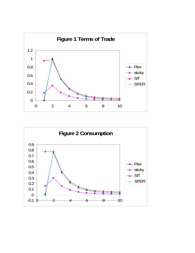
Figure 1 Terms of Trade

0

0.2

0.4

0.6

0.8

1

1.2

0 2 4 6 8 10

FlexstickySITSITER

Figure 2 Consumption

-0.10

0.10.20.30.40.50.60.70.80.9

0 2 4 6 8 10

FlexstickySITSITER

Figure 3 Employment

-2

-1

0

1

2

3

4

5

0 2 4 6 8 10

FlexstickySITSITER

Figure 4 Investment

-1

0

1

2

3

4

5

0 2 4 6 8 10

FlexstickySITSITER

30

Appendix

In this Appendix we describe the structure of the economy with endogenous investment that is

used to derive the results of Section 5.

Households

Household preferences are exactly as in the earlier sections, defined over consumption of traded

and non-traded goods and labor supply (negatively). Now however, households have the option of

investing in physical capital in the home country, either in the non-traded goods sector or the traded goods

sector. Household’s budget constraints may be written as:

(A1) 1

1 1( ) ( , ) ( ) (t

t t t Nt Tt t t t t t t KTt Tt KNt Nt ts S

PC P I I Q s s A s W L R K R K A s+

+ +∈

+ + + = + Π + + +∑ )

)

Households consume, invest in both types of capital, and purchase state contingent nominal bonds

1( tA s + (each of which pays off one dollar in state 1ts + ). They receive income from wages, profits from

ownership of firms in each sector, and rental income on their capital stock in each sector, as well as

payments on previously purchased state contingent nominal bonds. We abstract from household direct

holdings of money in this Appendix, as the monetary policies in Section 5 of the text are implemented

through interest rate rules.

Conditions (3.1) and (3.2) of the text hold as before (for each country’s households). In addition,

households choose investment in each sector to maximize utility, subject to the budget constraint (A1)

and the capital accumulation equations (5.1) and (5.2). The Euler equations for optimal accumulation of

capital in the non-traded and traded goods sectors, respectively, may be written as:

(A2) 11 1

1

( (1 )KNtNt t t t Nt

t

Rq C E C qP

ρ ρβ δ− − ++ +

+

= + − ) ,

(A3) 11 1

1

( (1 )KTtTt t t t Tt

t

Rq C E C qP

ρ ρβ δ− − ++ +

+

= + − ) ,

where we define 1'( )NtNt

Nt

IqK

φ −= and 1'( )TtTt

Tt

IqK

φ −= as the real relative price of capital, in terms of

consumer goods.

From the households’ choice of state contingent bonds, we may define a risk-free nominal

interest rate term as:

(A4) ( )1

1 11

1 ,t

tt t t t t

s St t

PQ s s C E CR P

ρ ρβ+

−+ +

∈ +

≡ =∑ .

The monetary policy rules are defined as in (4.6).

1

Firms

Firms hire labor and capital to minimize costs, subject to meeting demand for their goods at their

pre-set prices. Cost-minimizing firms in the non-traded goods sector will satisfy:

(A5) (1 ) Ntt Nt t

Nt

YW MCH

θ α= − ,

(A6) NitNt Nt t

Nt

YR MCK

θ α= ,

where NtMC is defined as the (common) marginal cost that is faced by each firm in the non-traded goods

sector. A similar pair of conditions is satisfied for firms in the traded goods sector, and an analogous set

of equations holds for the foreign country.

As in Section 4, firms set prices within the standard Calvo style pricing structure, where each firm

can change its price with probability 1 κ− . The optimal price of the price setting firm is identical to

condition (4.1), except that t i

t i

Wθ

+

+

is replaced by N t i

t i

MCθ

+

+

for the non-traded goods firm, and T t i

t i

MCθ

+

+

for

the traded goods firm.

Solution

The model is solved using a standard method of linearization around a non-stochastic steady

state. The calibrated parameter values are given in Table A1. We assume a unit inter-temporal elasticity

of substitution in preferences, and a unit elasticity of substitution between traded and non-traded goods.

The share of traded goods in preferences, γ , is set at 0.5. The discount factor is set at 0.99 on a quarterly

basis. The share of capital in income in both sectors is set at 0.36. The capital adjustment cost function is

calibrated so that the elasticity of q to the investment capital ratio is equal to 0.3, a standard value in the

literature. The rate of capital depreciation is set at 0.025 per quarter. Finally, we set κ = 0.75, so that on

average, prices are set for four quarters.

Table A1

ρ 1 φ(.) ln 0.3ln( / )

qI K

∂=

∂

γ 0.5 δ 0.025

β 0.99 κ 0.75

α 0.36

2