
Expander Graphs and Kazhdan’s Property (T)
65
Expander Graphs and Kazhdan’s Property (T) Giles Gardam An essay submitted in partial fulfillment of the requirements for the degree of B.Sc. (Honours) Pure Mathematics University of Sydney October 2012
Transcript of Expander Graphs and Kazhdan’s Property (T)

Expander Graphs and
Kazhdan’s Property (T)
Giles Gardam
An essay submitted in partial fulfillment ofthe requirements for the degree of
B.Sc. (Honours)
Pure Mathematics
University of Sydney
October 2012


Contents
Introduction . . . . . . . . . . . . . . . . . . . . . . . . . . . . . . . . . . . . . . . . . . . . . . . . . . . . . . . . . . . . . . . . . . . . . . . . iv
Acknowledgements . . . . . . . . . . . . . . . . . . . . . . . . . . . . . . . . . . . . . . . . . . . . . . . . . . . . . . . . . . . . . . . . . vi
Chapter 1. Expander Graphs . . . . . . . . . . . . . . . . . . . . . . . . . . . . . . . . . . . . . . . . . . . . . . . . . . . . 11.1. Graph Theory Background . . . . . . . . . . . . . . . . . . . . . . . . . . . . . . . . . . . . . . . . . . . . . . . . . . . . 11.2. Introduction to Expander Graphs . . . . . . . . . . . . . . . . . . . . . . . . . . . . . . . . . . . . . . . . . . . . . 51.3. Diameter in Expanders. . . . . . . . . . . . . . . . . . . . . . . . . . . . . . . . . . . . . . . . . . . . . . . . . . . . . . . . 81.4. Alternative Definitions of Expansion . . . . . . . . . . . . . . . . . . . . . . . . . . . . . . . . . . . . . . . . . . 101.5. Existence of Expanders . . . . . . . . . . . . . . . . . . . . . . . . . . . . . . . . . . . . . . . . . . . . . . . . . . . . . . . 131.6. Cayley Graphs . . . . . . . . . . . . . . . . . . . . . . . . . . . . . . . . . . . . . . . . . . . . . . . . . . . . . . . . . . . . . . . . 141.7. Some Negative Results for Cayley Graph Expansion . . . . . . . . . . . . . . . . . . . . . . . . . . . 151.8. Expansion in SL(2,Z/pZ) . . . . . . . . . . . . . . . . . . . . . . . . . . . . . . . . . . . . . . . . . . . . . . . . . . . . . 17
Chapter 2. Random Walks on Expanders . . . . . . . . . . . . . . . . . . . . . . . . . . . . . . . . . . . . . . 192.1. Random Walks and the Graph Spectrum. . . . . . . . . . . . . . . . . . . . . . . . . . . . . . . . . . . . . . 192.2. Spectral Expansion . . . . . . . . . . . . . . . . . . . . . . . . . . . . . . . . . . . . . . . . . . . . . . . . . . . . . . . . . . . 202.3. Efficient Error Reduction for RP . . . . . . . . . . . . . . . . . . . . . . . . . . . . . . . . . . . . . . . . . . . . . . 23
Chapter 3. Kazhdan’s Property (T) . . . . . . . . . . . . . . . . . . . . . . . . . . . . . . . . . . . . . . . . . . . . 273.1. Unitary Representations of Locally Compact Groups . . . . . . . . . . . . . . . . . . . . . . . . . . 273.2. Property (T). . . . . . . . . . . . . . . . . . . . . . . . . . . . . . . . . . . . . . . . . . . . . . . . . . . . . . . . . . . . . . . . . . 333.3. Compact Groups Have Property (T) . . . . . . . . . . . . . . . . . . . . . . . . . . . . . . . . . . . . . . . . . . 373.4. Kazhdan Sets and Generation . . . . . . . . . . . . . . . . . . . . . . . . . . . . . . . . . . . . . . . . . . . . . . . . . 413.5. Lattices and Property (T). . . . . . . . . . . . . . . . . . . . . . . . . . . . . . . . . . . . . . . . . . . . . . . . . . . . . 443.6. Some Non-compact Kazhdan Groups . . . . . . . . . . . . . . . . . . . . . . . . . . . . . . . . . . . . . . . . . . 46
Chapter 4. Constructions of Expanders . . . . . . . . . . . . . . . . . . . . . . . . . . . . . . . . . . . . . . . . 514.1. Kazhdan Expanders. . . . . . . . . . . . . . . . . . . . . . . . . . . . . . . . . . . . . . . . . . . . . . . . . . . . . . . . . . . 514.2. Margulis’s Construction of Expanders . . . . . . . . . . . . . . . . . . . . . . . . . . . . . . . . . . . . . . . . . 54
Appendix A. Asymptotic Representations . . . . . . . . . . . . . . . . . . . . . . . . . . . . . . . . . . . . . 56
Appendix B. A Lemma in Topology . . . . . . . . . . . . . . . . . . . . . . . . . . . . . . . . . . . . . . . . . . . . 57
References. . . . . . . . . . . . . . . . . . . . . . . . . . . . . . . . . . . . . . . . . . . . . . . . . . . . . . . . . . . . . . . . . . . . . . . . . . . 58
iii
Introduction
Expanders are highly connected sparse graphs of fundamental interest in mathematicsand computer science.
While it is relatively simple to prove the existence of expanders using probabilistic ar-guments in the style of Erdos, their explicit construction is difficult. The first explicit con-struction was given by Margulis in [Mar75], and employed Kazhdan’s Property (T) from therepresentation theory of semisimple groups. The aim of this essay is to present an essentiallycomplete exposition of the theory leading to the Margulis construction, while concurrentlydeveloping the most important and illustrative general theory of both expander graphs andProperty (T). We also present an application of expanders to derandomization.
Chapter 1 introduces expander graphs under several common definitions which we showto be equivalent, and gives some first properties of expanders. We also show the existenceof expanders, and consider some algebraic obstructions to groups giving expanders via theirCayley graphs.
Chapter 2 then gives an equivalent algebraic definition of expansion, in terms a graph’sadjacency matrix, and shows that expanders for this definition are expanders for the com-binatorial definitions of the preceding chapter. We consider random walks on an expandergraph, and study the relationship between the graph spectrum and the behaviour of suchrandom walks. The algebraic definition allows us to give a straightforward application of ex-panders to complexity theory, namely the derandomization of algorithms, where one improvesthe accuracy of a randomized computational procedure with very little need for additionalrandomness.
Property (T) is then introduced in Chapter 3. We develop some first consequences ofthe definition, demonstrated by many examples of groups which do not have Property (T)(with the help of amenability). After proving that all compact groups have Property (T) weconsider Kazhdan sets, which can be used to give an alternative definition of Property (T)and are essential for the construction of expanders. We then study lattices in groups withProperty (T); finite generation of these lattices was the original motivation for the formu-lation of Property (T). Finally, we give the proofs that certain non-compact groups haveProperty (T), which will be used in Chapter 4 to give constructions of expanders.
This work is mostly based on the books by Lubotzky [Lub94] and de la Harpe andValette [dlHV89], with the chapter on random walks and derandomization based on thesurvey paper [HLW06] of Hoory, Linial and Wigderson. The more recent and much largerwork of Bekka, de la Harpe and Valette on Property (T) in English, [BdlHV08], is alsoreferred to occasionally.
We present the material so as to be accessible for students of pure mathematics at honourslevel. Efforts have been made in the selection of content so as to give a broad yet gentleintroduction to the topics of Chapters 1, 2 and 3, while still leading fairly directly to a
iv

proof of the construction of expanders in Chapter 4. The proof that these constructions areexpanders is complete except for classical results regarding lattices, and relative property (T)of the pair (R2oSL(2,R),R2) for which we only give a proof outline. There are several otherparts of this essay where we call upon powerful results which we cannot prove here, but theseare not required for the construction of expanders and are used only to develop more generaltheory.
The books [dlHV89] and especially [Lub94] are written at an advanced level, and leavemuch unsaid. As well as filling in the details and correcting some erroneous arguments, ourtreatment includes many examples, remarks and original figures that give context to thenon-specialist, motivate results and proofs, and address potential barriers to understanding.We also avoid developing some technical machinery — such as weak containment of repre-sentations, induced representations, the Fell topology, and functions of positive type — asalthough these would be very useful topics for a detailed study of Property (T), that is notour main purpose.
In particular, in [Lub94] the proof of existence of expanders, Theorem 1.45 in the presentessay, contains several ‘easy to see’ claims which are actually erroneous in certain cases and sothe statement has been corrected here. The proof that compact groups have Property (T) inSection 3.3 differs from the literature in order to require fewer external results and to illustrateProperty (T) more concretely. The theory of random walks, including an application ofexpanders to derandomization, which forms Chapter 2, leads naturally to the spectral theoryof graphs and gives an interesting background to Margulis’s construction in Chapter 4.We also present the results of original computations investigating growth in the groupsSL(2,Z/pZ) in Section 1.8.
v

Acknowledgements
I would like to express my gratitude to several people. First and foremost I thank mysupervisor, Dr Anne Thomas, for her assistance throughout this project. She has beenincredibly helpful, patient and encouraging, and this essay has benefited enormously fromher meticulous editing. I am indebted to my family and Lisa for their love and support. Iwould like to acknowledge the support of Donald Jamieson, St Andrew’s College, The Schoolof Mathematics and Statistics and The University of Sydney throughout my degree. Manythanks also to Dr Neil Saunders for helpful comments on the manuscript, and to Dr EmmaCarberry for coordinating the pure mathematics honours programme.
vi

Chapter 1
Expander Graphs
This chapter introduces some common definitions of expanders and establishes theirequivalence, as well as proving that expanders have various properties. We also establish theexistence of expander graphs, and demonstrate some algebraic properties that are necessaryconditions for groups to have Cayley graphs that are expanders.
We begin with Section 1.1 covering the necessary background knowledge from graphtheory. Section 1.2 then gives our main definition of expanders (Definition 1.14), which makesprecise the slogan that expanders are highly connected sparse graphs. This is followed bysome examples and first results. Section 1.3 examines the relationship between expansion anddiameter, concluding with a proof that expanders have logarithmic diameter (Corollary 1.31).We then introduce in Section 1.4 some alternative definitions of expansion and show theirequivalence (Corollary 1.37). We develop a model of random regular graphs in Section 1.5 inorder to say in Theorem 1.45 that, under this model, almost all regular graphs are expanders.This establishes the existence of expanders. Section 1.6 introduces Cayley graphs as auseful means to construct regular graphs via group theory, with several examples. We provein Section 1.7 some negative results for expansion of certain families of Cayley graphs inTheorems 1.51 and 1.53. This algebraic result demonstrates the difficulty of constructingexpanders. Finally in Section 1.8 we present the results of original computations that exploreexpansion in the Cayley graphs of SL(2,Z/pZ) and in particular their diameters, which arethe subject of an open problem due to Lubotzky, Problem 1.58.
1.1. Graph Theory Background
A graph is a simple abstract representation of a collection of objects and their relation-ships. There are several different flavours of graphs; we begin with the following definition,and introduction variations afterwards as required.
Definition 1.1 (Graph). A graph X = (V,E) is a pair of sets V and E such that E ⊆ V ×V .The elements of V are called vertices, and the elements of E are called edges. A graph withthe edges being ordered pairs of vertices is directed. If we instead consider the edges to beunordered pairs of elements of V , then it is undirected. Edges of the form (v, v) are calledloops. If a graph is undirected and has no loops, we call it simple. If there is an edge (v, w),we say that the vertices v and w are adjacent and that the edge (v, w) is incident to thevertices v and w.
We often sketch graphs like polygons, or perhaps with curved rather than straight edges,but it is important to remember that the geometry of a particular sketch is not important(at least not in general, and not for our purposes here).
Examples 1.2. The following undirected graphs are shown in Figure 1.1.
1

0
17
2
3
4
5
6
0
1
2
3
4
5
6
7 000
001
010100
011101
110
111
Figure 1.1. The graphs C8, K8 and Q3, which all have 8 vertices.
a) The cycle graph on n ≥ 3 vertices, denoted Cn, is a graph with vertices V = Z/nZ =0, 1, 2, . . . , n− 1 and edges joining each i to i+ 1.
b) The complete graph on n vertices, denoted Kn, has an edge joining every pair of
distinct vertices. It has(n2
)= n(n−1)
2edges, which is maximal for an undirected
graph.c) The nth hypercube graph, denoted Qn, on 2n vertices, has vertex set 0, 1n, and
edges joining those n-tuples that differ in exactly one coordinate. It can be identifiedwith the 1-skeleton (that is, the vertices and edges) of the n-dimensional cube, soin particular the graph Q3 can be identified with the 1-skeleton of the familiar cube(which has 8 vertices and 12 edges in both the geometric and graph-theoretic senses).
It will be necessary sometimes to loosen our definition of a graph to the more generalnotion of a multigraph, where two vertices can be connected by multiple edges. We willindicate when this generalisation is required, but most of the examples we encounter willbe graphs rather than multigraphs. A multiset is a generalized set where the elementsare allowed to appear more than once (that is, they can have arbitrary positive integermultiplicity).
Definition 1.3 (Multigraph). A multigraph X = (V,E) is a pair consisting of a set V anda multiset E such that the elements of E are all members of V × V .
If a graph is simple, it is implicit that it is not a multigraph.Expanders are “sparse graphs”, in a sense that is made precise by the definition of degree.
See Remark 1.6 below.
Definition 1.4 (Degree, Regular). The degree of a vertex is the number of edges of Xincident to it. If all vertices in a graph X have degree k, we say X is a k-regular graph. Agraph is regular if it is k-regular for some non-negative integer k.
Examples 1.5. All cycle graphs are 2-regular, the complete graph Kn is (n−1)-regular andthe hypercube graph Qn is n-regular.
Remark 1.6. There is no precise, universally agreed-upon definition of “sparseness” forgraphs. It means roughly speaking that the total number of edges is much less than thenumber of unordered pairs on n vertices, that is
(n2
), which for a simple graph on n vertices
is the maximum number of edges possible. To give one possible precise definition, for an
2

infinite family of graphs (Vi, Ei) we could say that the total number of edges grows sub-quadratically (that is, |Ei|/|Vi|2 → 0 as i→∞), but for expanders we will require degree tobe constant, so that the total number of edges is O(|V |). (Readers unfamiliar with big-ohnotation should refer to Appendix A.)
Remark 1.7. While the theory of infinite graphs is interesting, covering such rich topics asCayley graphs for infinite groups and automorphism groups of trees, from now on we restrictattention almost exclusively to finite graphs, as these are the graphs for which expansion isdefined.
There are many different connectivity notions for graphs, which form an essential partof graph theory. The edges connecting vertices are the fundamental structure that graphshave beyond simply being sets, so in some sense the connectivity properties are the raisond’etre of graphs.
The most basic connectivity property we could ask of a graph is simply called connect-edness.
Definition 1.8. A walk between two vertices v and w in a graph is a sequence of vertices
v = v0, v1, . . . , vl−1, vl = w
such that vi is adjacent to vi+1 for i = 0, 1, . . . , l− 1. The length of such a walk is l. A walkis called a path if the vertices are pairwise distinct, that is, vi 6= vj whenever i 6= j. Twovertices v and w in a graph X = (V,E) are said to be connected if there is a path joiningthem (or, equivalently, if there is a walk joining them). If all pairs of vertices v, w ∈ V areconnected, we say that the graph X is connected.
If a graph is not connected, it is often convenient to discuss its connected components.For the definition of connected components, we note that in an undirected graph, the relationof connectedness is an equivalence relation on the set V of vertices: symmetry holds by takinga path of length zero, reflexivity follows from taking a reversed path, and transitivity followsfrom concatenation of paths.
Definition 1.9. A connected component of an undirected graph is an equivalence class ofvertices under the equivalence relation of connectedness.
Connected graphs have a natural metric, usually referred to as distance. For unconnectedgraphs, we can consider two unconnected vertices to be at distance +∞ from each other,but this is not actually a metric because the distances in a metric space must be finite bydefinition (although with the natural addition in R+
0 ∪ +∞ the axioms for a metric stillhold).
Definition 1.10. The distance between two vertices v and w in a graph, denoted d(v, w),is the length of the shortest path joining them. The distance from v to a subset A ⊆ V ofthe vertices of the graph is defined to be
d(v,A) = minw∈A
d(v, w).
Since the distance function on a graph is a “local” property of the graph (pertaining onlyto the two vertices directly, and to the vertices joining them in a shortest path indirectly),it is often natural to discuss its global maximum.
3
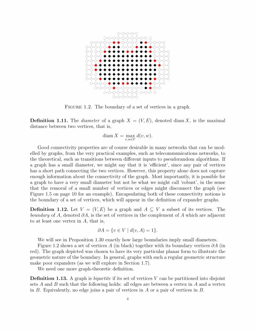
Figure 1.2. The boundary of a set of vertices in a graph.
Definition 1.11. The diameter of a graph X = (V,E), denoted diamX, is the maximaldistance between two vertices, that is,
diamX = maxv,w∈V
d(v, w).
Good connectivity properties are of course desirable in many networks that can be mod-elled by graphs, from the very practical examples, such as telecommunications networks, tothe theoretical, such as transitions between different inputs to pseudorandom algorithms. Ifa graph has a small diameter, we might say that it is ‘efficient’, since any pair of verticeshas a short path connecting the two vertices. However, this property alone does not captureenough information about the connectivity of the graph. Most importantly, it is possible fora graph to have a very small diameter but not be what we might call ‘robust’, in the sensethat the removal of a small number of vertices or edges might disconnect the graph (seeFigure 1.5 on page 10 for an example). Encapsulating both of these connectivity notions isthe boundary of a set of vertices, which will appear in the definition of expander graphs.
Definition 1.12. Let V = (V,E) be a graph and A ⊆ V a subset of its vertices. Theboundary of A, denoted ∂A, is the set of vertices in the complement of A which are adjacentto at least one vertex in A, that is,
∂A = v ∈ V | d(v,A) = 1.
We will see in Proposition 1.30 exactly how large boundaries imply small diameters.Figure 1.2 shows a set of vertices A (in black) together with its boundary vertices ∂A (in
red). The graph depicted was chosen to have its very particular planar form to illustrate thegeometric nature of the boundary. In general, graphs with such a regular geometric structuremake poor expanders (as we will explore in Section 1.7).
We need one more graph-theoretic definition.
Definition 1.13. A graph is bipartite if its set of vertices V can be partitioned into disjointsets A and B such that the following holds: all edges are between a vertex in A and a vertexin B. Equivalently, no edge joins a pair of vertices in A or a pair of vertices in B.
4

1.2. Introduction to Expander Graphs
In this section we give definitions of expander graphs and expander families, illustratedby some examples.
Throughout the rest of this chapter, we will adopt the following convention:
X = (V,E) is a k-regular graph on n vertices
for positive integers n and k.There are many different definitions of expander graphs, but they are all equivalent up to
a change of constant (possibly after some transformation). We will present the most commondefinitions and prove they are equivalent.
Our first and most important definition of expanders is as follows.
Definition 1.14 (Expander). Let c > 0. A finite k-regular graph X = (V,E) on n verticesis called an (n, k, c)-expander if for every subset of vertices A ⊆ V with |A| ≤ n
2,
(1.15) |∂A| ≥ c|A|.
If n and k are understood, then we will simply call X a c-expander.
Remark 1.16. Equation (1.15) means that sets A which are ‘not too large’ cannot haveboundaries that are very small relative to A. A condition like |A| ≤ n
2must be imposed,
because otherwise as A becomes a large proportion of V , ∂A can only be very small, andconsequently c would need to be very small for large graphs (in fact, if we allowed A = Vthis would force c = 0).
Lemma 1.17. Let X be a graph. Then X is a c-expander for some c > 0 if and only if Xis connected.
Proof. If a graph X is connected, then |∂A| > 0 whenever 0 < |A| < n, so since there areonly finitely many A ⊆ V , X will be a c-expander for
(1.18) c(X) := min0<|A|≤n
2
|∂A||A|
> 0.
If on the other hand X is not connected, letting A be a connected component of minimalsize in X we then have ∂A = ∅ and |A| ≤ n
2(since there must be at least 2 connected
components).
Remark 1.19. Although Lemma 1.17 completely classifies which graphs are expanders whentaken by themselves, we wish to find large sparse graphs with the expansion coefficient cbounded away from zero uniformly. It is applications of expanders that first motivated thefollowing definition. However, we can also motivate it by the observation it allows us tomove from the definition of single expander graphs, something which requires choosing anarbitrary c, to families of expanders which can be described more ‘qualitatively’, that is,without imposing some constant a priori.
Definition 1.20 (Family of expanders). Let k be a positive integer. Let (Xi) = ((Vi, Ei))be a sequence of k-regular graphs such that |Vi| → ∞ as i → ∞. We say that (Xi) is anexpander family if there is some c > 0 such that each graph in this sequence is a c-expander.
5

Figure 1.3. A graph X with poor expansion.
Figure 1.3 presents a graph X which is a manifestly poor expander. If we take theset A in Definition 1.14 to be the ‘cluster’ of vertices on the left, then we have |∂A| = 1,but A comprises half of the vertices. Since X is connected, it will be a c-expander for somesufficiently small positive c. However, the best possible c will be very small for a graph of thissize, and we can imagine that if we had a sequence of graphs of increasing size with similarstructure (only one edge connecting the two ‘sides’ of the vertex set) then their respectiveconstants c would tend to 0. (Unsurprisingly, the technical term for an edge, like the onejoining the two sides in Figure 1.3, whose deletion disconnects the graph, is a bridge.)
Example 1.21. The sequence (Kn) of complete graphs is not an expander family becausetheir degree is not constant.
Lemma 1.22. The sequence of cycle graphs (Cn) with n ≥ 3 is not an expander family.
Proof. Take A in Definition 1.14 to be the vertices on a path of length bn2c. Then if Cn is
a c-expander, we must have
c ≤ |∂A||A|
=2
bn2c
= O(1/n)
as n→∞.
Corollary 1.23. A family of k-regular expanders must have k ≥ 3.
Proof. As expanders are connected, they must have degree at least 2, except for the case ofgraphs on 2 vertices (degree 1 graphs have the form of an even number of vertices connectedin disjoint pairs). However, up to isomorphism, the only connected 2-regular graph on n ≥ 3vertices is the cycle graph Cn.
Remark 1.24. As is common practice, we will abuse nomenclature and say that graphsthemselves are expanders to mean that they form a family of expanders, and likewise whensaying that graphs are not expanders (even though, as noted above, all connected graphsare automatically c-expanders for some sufficiently small c, and could in fact be realised asa member of an expander family by simply adding them to any existing expander family).For example, we say that cycle graphs are not expanders.
Remark 1.25. It turns out that there are in fact expanders of degree 3 (and in certain modelsof random regular graphs, almost all 3-regular graphs are expanders [HLW06, Theorem4.16]). As a constructive example, for each prime p we construct a graph whose vertex set
6

Figure 1.4. 3-regular expanders on 13, 37 and 97 vertices.
is Fp = Z/pZ, with an edge joining each vertex x to x − 1, x + 1 and x−1 (taking 0 to beits own inverse). This graph is illustrated in Figure 1.4 for the sequence p = 13, 37, 97.These graphs are a family of expanders, indexed by the primes p. However the proof ofexpansion depends on the Selberg 3/16 Theorem, a deep result from number theory (see[Lub94, p.53] for details). We need to defer to Selberg’s theorem because SL(2,Z) does nothave Property (T), and so we cannot use Margulis’s construction directly (Proposition 4.1,see also Remark 4.7). Note that while this is an explicit construction from a mathematicalpoint of view, it is described in [HLW06, p.453] as being only ‘mildly explicit’ (in a precisesense defined in that paper) since there is no known efficient deterministic algorithm togenerate large primes.
Remark 1.26. An alternative way of defining expander families to Definition 1.20 wouldbe to require that
lim infi→∞
c(Xi) > 0
where c is as defined by Equation (1.18). Naturally, it is possible that a sequence (Xi) ofgraphs is not an expander family for the reason that there is no uniform lower bound on thec(Xi), even though the sequence of graphs (Xi) still has a subsequence that is an expanderfamily (consider for example the sequence of constants 0, 1, 0, 1, . . .). In this essay, wheneverwe claim that a sequence of graphs is not an expander family, we will in fact show specificallythat limi→∞ c(Xi) = 0, so that no subsequence gives an expander family.
Remark 1.27. There is a straightforward upper bound on the expansion constant c in theinequality (1.15). As ∂A ⊆ V \ A, we have |∂A| ≤ n − |A|. Thus for any A ⊆ V of an(n, k, c)-expander, if |A| = bn/2c then we have
c ≤ |∂A||A|≤ n− bn/2c
bn/2c=
1 if n is even;
1 + 2n−1 if n is odd.
7

In a complete graph Kn, the inequalities become equalities, and for any smaller A, thatis |A| < bn/2c, we have |∂A|/|A| > c. Thus the upper bound on c is tight.
1.3. Diameter in Expanders
We have already mentioned that good expansion guarantees that a graph is both ‘robust’and ‘efficient’, which respectively mean that it is not easily disconnected and that any pairof vertices has a small distance between them. In this section we pursue the second of thosenotions in detail. We first define balls and spheres in graphs, which will be used to studygrowth, and show that the boundary of a ball is a sphere. After this setup, we show inProposition 1.30 and Corollary 1.31 that expanders have logarithmic diameter, and discussthe significance of this result.
Definition 1.28 (Balls and spheres). Let X = (V,E) be a connected, undirected graph withmetric d as defined in Definition 1.10. Let v ∈ V be a vertex of X, and r a non-negativeinteger. The ball of radius r centred at v is defined to be
Br(v) = w ∈ V | d(v, w) ≤ r.
The sphere of radius r centred at v is defined to be
Sr(v) = w ∈ V | d(v, w) = r.
It is immediate from this definition that the balls partition into spheres:
Br(v) =r⋃
r′=0
Sr′(v).
The following result, however, does require proof (for example, it is not true for arbitrarymetric spaces whose distances are integral).
Lemma 1.29. Let v be a vertex of an undirected graph X, and r ∈ N. Then
∂Br(v) = Sr+1(v).
Proof. First let w ∈ ∂Br(v). By the definition of boundary, w /∈ Br(v), so d(v, w) > r, andthere is a w′ ∈ Br(v) such that d(w′, w) = 1. Then by the triangle inequality,
d(v, w) ≤ d(v, w′) + d(w′, w) ≤ r + 1.
Thus d(v, w) = r + 1, so w ∈ Sr+1(v).Now let w ∈ Sr+1(v). Then there is a path w,w′, . . . , v in X of length r+ 1 from w to v,
and for this w′ we have d(w,w′) = 1. This path also gives a path of length r from w′ to v, sothat w′ ∈ Br(v). As Br(v) and Sr+1(v) are disjoint, d(w,Br(v)) > 0. Thus d(w,Br(v)) = 1,that is, w ∈ ∂Br(v).
Proposition 1.30. Let X = (V,E) be an (n, k, c)-expander. Then
diam(X) ≤ 2
log(1 + c)log n.
The proof we now present follows [KS11, p.97].
8

Proof. Let v1, v2 ∈ V be two arbitrary vertices of X. Because X is an expander it isconnected. So any vertex w ∈ V is joined to v1 by a path, which must have length atmost n − 1 (by definition, a path consists of distinct vertices). So d(v1, w) ≤ n − 1. HenceBn−1(v1) = V and thus
v1 = B0(v1) ⊆ B1(v1) ⊆ B2(v1) ⊆ · · · ⊆ Bn−1(v1) = V.
Since |V | > n2
we can then define r1 to be the least positive integer r such that
|Br(v1)| >n
2.
Define r2 similarly, with respect to v2. For any r < r1 we have |Br(v1)| ≤ n2, so by Lemma 1.29
and the expansion of X we have
|Br+1(v1)| = |Br(v1)|+ |Sr+1(v1)|= |Br(v1)|+ |∂Br(v1)|≥ (1 + c)|Br(v1)|.
As |B0(v1)| = 1, a trivial induction gives
|Br1(v1)| ≥ (1 + c)r1 .
Since |Br1(v1)| ≤ n, we now have
r1 ≤ log1+c n =log n
log(1 + c)
and similarly the same upper bound holds for r2.Because |Br1(v1)|+ |Br2(v2)| > n, these two balls cannot be disjoint, that is, there exists
w such that d(v1, w) ≤ r1 and d(v2, w) ≤ r2. Thus
d(v1, v2) ≤ d(v1, w) + d(w, v2) ≤2
log(1 + c)log n.
As v1 and v2 were arbitrary, we conclude that
diam(X) ≤ 2
log(1 + c)log n.
Corollary 1.31. (Expanders have logarithmic diameter) Let (Xi) = ((Vi, Ei)) be a familyof expanders. Then
diam(Xi) = O(log |Vi|).
Remark 1.32. This corollary is a very simple example of the kind of results that followfrom the definition of an expander family. In this way, it validates the definition of expanderfamilies. It is only because we have a fixed lower bound on the expansion constants of all thegraphs Xi that we can make such a statement: the big-oh notation hides a constant whichdepends on the constant of expansion c.
Remark 1.33. The diameter of expanders is optimal in the sense that any family of graphswhere the vertices have uniformly bounded degree must have at least logarithmic diameter.The proof of this is very similar to the proof of Proposition 1.30 above, noting that if k isan upper bound on degree then |∂A| ≤ (k + 1)|A| for all A ⊆ V . One might wonder if the
9

Figure 1.5. The ball of radius 6 in the 3-regular tree.
converse to Corollary 1.31 holds, that is, whether a family of graphs of logarithmic diameteris necessarily a family of expanders. The converse however is false, and it is not too difficultto find families of graphs with logarithmic diameter that are not expanders. (Indeed, sincethe problem of constructing expanders turns out to be so difficult, constructing such counter-examples is essentially the same problem as finding large regular graphs with logarithmicdiameter.) A very natural way to construct such examples is to take symmetric trees ofconstant degree for internal vertices and join the leaves to fill them out to be regular. Asthe simplest example, we can take balls of radius r inside the 3-regular tree, joining theleaf nodes in local cycles of length 4, as illustrated for r = 6 in Figure 1.5. The number ofvertices in the balls grows exponentially in r, whereas the diameters of the balls are 2r, sothat they have logarithmic diameter. On the other hand, if we take A in Definition (1.14) asone particular branch at the root, comprising roughly 1/3 of the vertices but with boundary∂A containing only the root, we see that these graphs will not form a family of expanders.So in summary, expansion is strictly stronger than logarithmic (that is, optimal) diameter.
1.4. Alternative Definitions of Expansion
In this section, we consider ‘edge expansion’, the expansion of a graph in terms of thenumber of edges connecting a subset of its vertices to the rest of the graph, as opposed toDefinition 1.14 which we might call ‘vertex expansion’. After this, we consider a definitionof expansion for bipartite graphs. We will show that these definitions are all equivalent, upto suitable change of constants and transformations.
Definition 1.34 (Edge expansion). Let X = (V,E) be a finite graph. Define the Cheegerconstant (or isoperimetric constant) of X, denoted h(X), by
h(X) = minAtB=V
|E(A,B)|min(|A|, |B|)
where the (outer) minimum runs over all partitions V = A t B, and E(A,B) is the set ofedges between vertices in A and vertices in B.
10

Remark 1.35. We call h(X) the Cheeger constant in analogue with the Cheeger constantof a Riemannian manifold M , the minimal ratio of the area of a hypersurface that dividesM into two disjoint pieces to the smaller of the volumes of those pieces (see [Cha84, p.95]for further details). We will see in the next chapter that the analogy is not superficial, andthat bounds relating the Cheeger constant of a manifold to the eigenvalues of its Laplacianhave their counterparts for the Cheeger constant of a finite graph and the eigenvalues of itsadjacency matrix (or, equivalently, the graph Laplacian).
We could now define an expander family to be a sequence (Xi) of graphs such that thesequence (h(Xi)) of Cheeger constants is bounded away from zero. Naturally, we would liketo know if this is equivalent to our previous definition of an expander family (Definition 1.20).The following proposition relates the different expansion constants of a single graph, whichwill give us the desired equivalence of definitions of expander families.
Proposition 1.36 (Bounds between expansion constants). For a k-regular graph X,
h(X)
k≤ c(X) ≤ h(X).
Proof. Suppose V = AtB is a partition of the vertices. Without loss of generality, we mayassume that |A| ≤ |B| and thus |A| ≤ n
2.
Since to each vertex b ∈ ∂A ⊆ B there corresponds at least one edge (a, b) ∈ E(A,B),we have |∂A| ≤ |E(A,B)|.
As X is k-regular, for each vertex b ∈ ∂A there are at most k edges incident to b, and inparticular there can be at most k edges of the form (a, b) ∈ E(A,B). Thus |E(A,B)| ≤ k|∂A|.
Putting these together, we have
1
k· |E(A,B)|
min(|A|, |B|)≤ |∂A||A|≤ |E(A,B)|
min(|A|, |B|).
As this holds for any partition with |A| ≤ n2, taking minima over all such partitions gives
1
kh(X) ≤ c(X) ≤ h(X).
Corollary 1.37 (Equivalence of vertex and edge expansion). Vertex and edge expansionare equivalent, that is, a family of k-regular graphs is a family of vertex expanders (in thesense of Definition 1.14) if and only if it is a family of edge expanders (that is, the Cheegerconstants as defined in Definition 1.34 are bounded away from zero).
Remark 1.38. Note that the equivalence of vertex and edge expansion depends very essen-tially on the fact that the degree of vertices is bounded (actually a constant k). For example,the trees of diameter 2, which are also known as the star graphs, in which one central vertexis joined to all the other vertices, have good edge expansion but poor vertex expansion.
Our third and final combinatorial definition of expanders is for bipartite graphs. Whilewe will only use this definition for the proof of existence below, it is useful in general, andtheoretical computer scientists are mostly interested in bipartite expanders. The followingdefinition is taken from [Lub94, p.2].
11

Definition 1.39 (Bipartite expanders). Let c > 0. An (n, k, c)-bipartite expander X =(V,E) is a bipartite, k-regular graph with V = I t O such that the edges go from I to O,|I| = |O| = n and for any A ⊂ I with |A| ≤ n
2we have
|∂A| ≥ (1 + c)|A|.(The two sets I and O are named for input and output.)
Compared with Definition 1.14, the idea is that since ∂A ⊆ O which is disjoint from I,rather than requiring the boundary ∂A to be not too small relative to A, we instead requireit to be larger by some fixed proportion.
We turn now to the equivalence of Definitions 1.39 and 1.14. Here we are using the term‘equivalence’ rather loosely; there is implicit transformation of graphs involved.
Moving from vertex expansion (Definition 1.14) to bipartite vertex expansion (Defini-tion 1.39) is straightforward. One simply takes the extended bipartite double cover.
Definition 1.40 (Bipartite double cover). Let X = (V,E) be a graph. The bipartite doublecover of X is a graph whose vertex set is
∪i∈0,1V = v0 : v ∈ V ∪ v1 : v ∈ V and which has two edges, of the form v0, w1 and v1, w0, corresponding to each edgev, w ∈ E.
The extended bipartite double cover of X is obtained by taking the bipartite double cover,and adding an edge v0, v1 for each vertex v ∈ V (which we may think of joining each vertexto its twin).
Remark 1.41. The bipartite double cover is indeed a 2-sheeted cover of the graph X as atopological space. This is also true for the bipartite double cover of a multigraph X.
Transforming a bipartite expander in the sense of Definition 1.39 into an expander as inDefinition 1.14 is more difficult. It requires identifying vertices in I with vertices in O. Aperfect matching in a bipartite graph is a partitioning of the vertices into pairs of adjacentsets (or alternatively, a subset E ′ of the edges such that each vertex is incident to preciselyone edge e ∈ E ′). Hall’s ‘Marriage Theorem’ can be phrased as follows:
Theorem 1.42 (Hall 1935, [Die00, Theorem 2.1.2]). Let X be a bipartite graph with edgesgoing between vertex sets I and O, where |I| = |O|. There exists a perfect matching in X ifand only if |∂A| ≥ |A| for all A ⊆ I.
Using this theorem (which we shall not prove),associate a distinct neighbour w ∈ O toevery v ∈ I. We note that applying the theorem does not actually need the expansionproperty, only the regularity of the graph (and |I| = |O| of course): the k|A| edges leavingA must hit at least |A| vertices in B, as each vertex in B is incident to at most k of theseedges. By identifying these pairs of the matching, we get a graph on n vertices.
Remark 1.43. The perfect matching whose existence is guaranteed by Hall’s Theorem is notcanonical. Moreover, different identifications can result in non-isomorphic quotient graphs,even for small cases such as the cycle graph C4.
Proposition 1.44. If a graph is a c-expander, then its extended double cover is a c-bipartiteexpander. If a graph is a c-bipartite expander, then the graph formed by identifying verticesin a perfect matching is a c-expander.
12

1.5. Existence of Expanders
Pinsker first showed the existence of expander graphs in [Pin73]. In the style of Erdos—who used probabilistic methods to establish the existence of various combinatorial objects— Pinsker considered a model of random regular graphs, and showed that the probabilitythat such a random graph is an expander is non-zero for sufficiently large n. In fact, theprobability tends to 1. In this section we follow the example of Pinsker and develop a modelof random regular graphs, and use it to prove the existence of expanders.
This line of thinking raises a natural but difficult question: how should one model arandom regular graph?
Perhaps a nice way to do this would be to consider each isomorphism class of k-regulargraphs on n vertices to be equiprobable. However, there is not even a known formula forthe number of such isomorphism classes in general! So we model a k-regular bipartite graphon 2n vertices as follows. The vertices are labelled I = v1, . . . , vn and O = w1, . . . , wn.We take k permutations π1, . . . , πk ∈ Sn, drawn uniformly (each permutation is chosen withprobability 1
n!) and independently. Then for each 1 ≤ i ≤ n and 1 ≤ j ≤ k we create an
edge joining vi and wπj(i). (The random graphs generated are very likely to be multigraphs:even for n = 2 we are just asking about the probability that a random permutation is aderangement, which is approximately 1/e.)
The following theorem is adapted from [Lub94, Proposition 1.2.1] (which in turn followsthe presentation in Sarnak’s book [Sar90, pp.64-65]). That proposition claims the result tohold true for k = 5, however the bound on probability actually diverges to infinity in thatcase, so the proofs are erroneous in the case k = 5. Moreover, it is claimed that a certainfunction R(t), which we will define below, is decreasing for 1 ≤ t < n
3. This claim is not
true, even after ignoring the small variations owing to the parity of t. (In fact, if k = 6 thenthe minimum of R(t) is at n
5approximately.) A proof with all the details would be too long
to include here; the reader is referred to [HLW06, pp.478-481]. We sketch the proof fromLubotzky’s book.
Theorem 1.45 (Existence of expander families). Let k ≥ 6 be a positive integer and c = 12.
Then the probability that a random k-regular multigraphs on n vertices, drawn from themodel described above, is a c-expander tends to 1 as n → ∞. In particular, families ofc-expanders exist.
Proof sketch. Consider sets A ⊆ I with |A| = t ≤ n2
and B ⊆ O with |B| = m = b32tc.
Let P (t) be the probability that for a random k-regular bipartite expander, ∂A ⊆ B. Wecompute that
P (t) =
(m!(n− t)!(m− t)!n!
)k.
Let Q(t) be the number of choices of such A and B. Then
Q(t) =
(n
t
)(n
m
).
13
Put R(t) = Q(t)P (t). Then a very crude upper bound on the probability that a randomk-regular bipartite graph on n vertices is not a c = 3
2expander is
Pn =∑
1≤t≤n2
R(t).
It now remains to show that Pn → 0 as n→∞.For small values of t, the probability P (t) is large whereas Q(t) is small. The opposite
is true for values more of the order of n3≤ t ≤ n
2. One can verify that R(t) is roughly
decreasing for small values, so the maximum occurs at R(1). For the large values, wecompare R(t) to R(n
2) which we can approximate to within a constant factor by Stirling’s
formula (Example A.8). Then for all t we have
R(t) ≤ R(1) +R(n
3
)+R
(n2
)= o
(1
n
)so that Pn → 0.
1.6. Cayley Graphs
Cayley graphs give a means to construct graphs from groups. The construction of ex-panders due to Margulis, which is the main objective of this essay and will be presented inChapter 4, is a family of Cayley graphs. There are many reasons why it is natural to useCayley graphs to construct expanders. As well as being regular graphs by definition, theyenable us to construct large graphs in an effective and concise manner; it can be much easierto describe the group than the graph. Before describing some previously-encountered graphsas Cayley graphs, we give the definition and some first remarks.
Definition 1.46 (Cayley Graph). The Cayley graph of a group G with respect to a gener-ating set S ⊆ G is the directed graph whose vertex set is G and whose edges are given by(g, gs) for each g ∈ G and s ∈ S. It is denoted by Cay(G,S).
Remark 1.47. The Cayley graph will be simple (that is, loop-free) if and only if 1 /∈ S.Since for any distinct s, s′ ∈ S we have gs 6= gs′, it follows that the edges of Cay(G,S)
are distinct (so it is not a multigraph).Because S generates G, every g ∈ G can be written as a word s1s2 · · · sl in the generators
S and their inverses, and is reachable from 1G by the path
1G, s1, s1s2, s1s2s3, . . . , s1s2 · · · sl = g.
Thus Cay(G,S) is connected.Finally, we say that S ⊆ G is symmetric if
S = S−1 := s−1 | s ∈ S.If S is symmetric, then we can identify Cay(G,S) with an undirected graph. This is becauseto each directed edge (g, gs) there corresponds a reversed edge
(gs, (gs)s−1) = (gs, g).
(This is still true if s−1 = s.) This undirected graph is |S|-regular. Usually, we will have S asymmetric generating set which does not include the identity, so that the graph Cay(G,S)is a simple, connected, undirected graph.
14

Remark 1.48. As expanders are finite graphs, we are only interested in the Cayley graphsof finite groups (note that the number of vertices in Cay(G,S) is |G|). These finite groupsmight, however, be obtained as subgroups or quotients of infinite groups, so it is certainlynot the case that we will consider only finite groups in this essay.
Remark 1.49. It is arguably more common to consider left group actions. The reason wedefine the Cayley graph by right-multiplication of the vertices g ∈ G by the generators s ∈ Sis so that the action of G on itself by left-multiplication induces a graph isomorphism (theelement h ∈ G maps any edge (g, gs) to the edge (hg, hgs)).
Examples 1.50. The families of graphs from Examples 1.2, which were illustrated in Fig-ure 1.1 on page 2, can be constructed as Cayley graphs as follows.
a) The Cayley graph for the group Z/nZ with respect to the generating set S = 1,−1is the cycle graph Cn.
b) The group Z/nZ taken with the generating set S = 1, 2, . . . , n− 1 consisting of allnon-zero elements has the Cayley graph Kn.
c) The Cayley graph for the direct product of n groups of order 2,
G =n⊕i=1
Z/2Z,
with the n generators
S = (1, 0, . . . , 0), . . . , (0, . . . , 0, 1)is the nth hypercube graph Qn.
As previously mentioned, none of these is an expander.
We will now turn to some general negative results for expansion of Cayley graphs.
1.7. Some Negative Results for Cayley Graph Expansion
As expanders resemble random graphs, we might expect that groups which are veryuncomplicated would not give expanders. In this section we will prove some results whichestablish the veracity of this intuition to some extent, first in the case that our particularnotion of ‘uncomplicated’ is ‘abelian’.
Theorem 1.51 (Abelian groups do not give expanders). Let (Gi) be a family of abeliangroups with respective generating sets Si of constant cardinality k. Then the graphs Cay(Gi, Si)are not a family of expanders.
Proof. We may assume without loss of generality that Si is symmetric, because we can takeSi ∪ S−1i otherwise (possibly taking some generators more than once so as to get 2k-regularCayley graphs). Let S = s1, . . . , sk. Then the balls in the graph can be written
Bm(0) =
a1s1 + · · ·+ aksk
∣∣∣∣∣ ai ≥ 0,k∑i=1
ai ≤ m
.
So the size of Bm(0) is bounded by the number of ways of writing an integer l ≤ m as thesum of non-negative integers a1, . . . , ak, summed over all possible l. For each fixed l, this issimply making an unordered selection of l objects of k types, with repetition allowed. (The
15

fact that this selection is unordered is very important, and is where the fact that the groupis abelian enters.) It is well-known that this is(
l + k − 1
k − 1
).
We can derive this result by noting that such selections of l objects of k types are in bijectionwith sequences of l + k − 1 symbols, k − 1 of which are −’s and which delimit the blockscomprising some of the l ’s, the blocks encoding how many of that particular item appears inthe selection. For example, the selection (1, 2, 0, 1) is represented by the sequence −−−.
We have (l + k − 1
k − 1
)≤ (l + k − 1)k−1
(k − 1)!≤ 2k
(k − 1)!lk−1
for l ≥ k − 1.We then have that
|Bm(0)| ≤m∑l=0
(l + k − 1
k − 1
)≤
k−1∑l=1
(l + k − 1
k − 1
)+
m∑l=k
2k
(k − 1)!lk−1 ≤ 2k
(k − 1)!mk + C
for a constant C. Thus |Bm(0)| = O(mk), where the implied constant depends only on k, andnot on the particular abelian group whose Cayley graph we are considering. However, theballs in an expander must grow exponentially (until the comprise at least half the vertices,which will only be an problem for finitely many of the Cayley graphs) as seen in the proofof Proposition 1.30. Thus Cay(Gi, Si) is not a family of expanders.
One can generalize Theorem 1.51 to solvable groups with Theorem 1.53. Solvable groupsare a class of groups which can be understood as being ‘approximately abelian’. We firstrecall the definition of solvable groups.
Definition 1.52. A group G is solvable if its derived series G(n), defined recursively byG(1) = G and G(n+1) = [G(n), G(n)], terminates at the trivial group after finitely many steps.That is, there exists a minimal positive integer l called the derived length of G such thatG(l) = 1.
Theorem 1.53. Let (Gi) be a sequence of finite groups with respective generating sets Siof constant cardinality k. Let l be a positive integer. Suppose that for all n, we have thatGi is solvable with derived length at most l. Then the graphs Cay(Gi, Si) are not a familyof expanders.
The theorem appears in Krebs and Shaheen [KS11, Theorem 4.47], and is originally dueto Lubotzky and Weiss [LW93, Corollary 3.3] (who give it as a corollary to a non-expansionresult for quotients of a finitely generated amenable group). We do not prove this theorem asit requires some inheritance results on Cayley graph expansion for subgroups and quotients,which despite not being difficult we do not develop here so as not to stray too far from ourpath towards the constructions of Chapter 4.
Example 1.54. Finite dihedral groups do not give expanders, as they have derived seriesof length 2.
16
Remark 1.55. Theorem 1.53 is essentially the only result known about when it is impossibleto choose generating sets to construct a family of expanders as the Cayley graphs of a givenfamily of groups [Kas09]. We will see that in contrast the Margulis construction does workfor any fixed set of generators of the group with Property (T) that is used.
The preceding remark on generators raises the question of whether expansion is in fact agroup property; Lubotzky and Weiss presented the problem as follows [LW93, Problem 1.1].
Problem 1.56. Let (Gi) be a family of finite groups, with 〈Si〉 = 〈S ′i〉 = Gi and |Si|, |S ′i| ≤k for all i. Does the fact that (Cay(Gi, Si)) is an expander family imply the same for(Cay(Gi, S
′i))?
This question was answered in the negative by Alon, Lubotzky and Wigderson in [ALW01].Their counterexample is beyond the scope of this essay. As noted in [HLW06, p.536], themore recent paper [Kas07] provides a simpler counterexample. In this paper Kassabov an-swered what had been a big open problem for decades, by demonstrating that for certaingenerating sets, the alternating groups An and symmetric groups Symn give expanders. How-ever, one can show that for instance, the generating sets Sn = (1 2), (1 2 . . . n)±1 do notmake Cay(Symn, Sn) expanders.
Remark 1.57. Expander families are defined by some texts to have uniformly bounded,rather than constant, degree. For instance, the original presentation of Problem 1.56 byLubotzky and Weiss was for uniformly bounded degree. However, this does not change theproblem essentially. In one direction, graphs with constant degree trivially have uniformlybounded degree. In the other direction, if a family of expanders has uniformly boundeddegree, we can add edges to obtain constant degree graphs (or, perhaps necessarily, constantdegree multigraphs), which only possibly improves their expansion properties.
As a technicality, if the bound on degree is k, we can generally just add an edge betweenvertices of degree less than k until each graph is k-regular, possibly introducing loops. How-ever, when nk is odd we will have to go to a (k + 1)-regular graph (the handshaking lemmarequires that the sum of degrees is even, being twice the number of edges).
Since we are mostly concerned with Cayley graphs, we will restrict attention to regulargraphs.
1.8. Expansion in SL(2,Z/pZ)
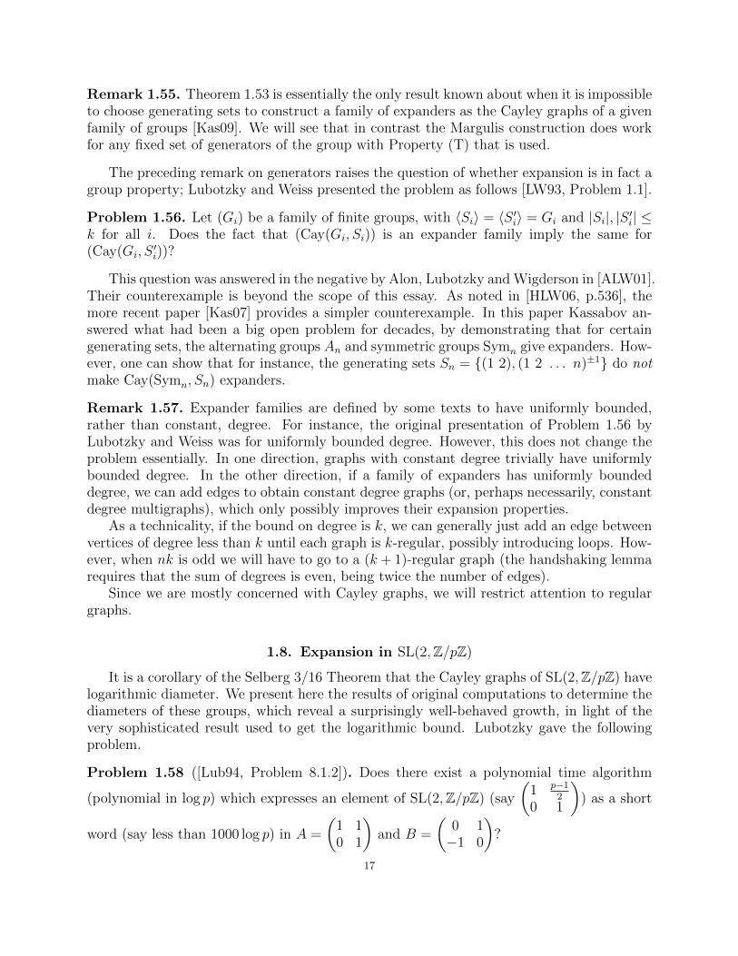
It is a corollary of the Selberg 3/16 Theorem that the Cayley graphs of SL(2,Z/pZ) havelogarithmic diameter. We present here the results of original computations to determine thediameters of these groups, which reveal a surprisingly well-behaved growth, in light of thevery sophisticated result used to get the logarithmic bound. Lubotzky gave the followingproblem.
Problem 1.58 ([Lub94, Problem 8.1.2]). Does there exist a polynomial time algorithm
(polynomial in log p) which expresses an element of SL(2,Z/pZ) (say
(1 p−1
20 1
)) as a short
word (say less than 1000 log p) in A =
(1 10 1
)and B =
(0 1−1 0
)?
17

Figure 1.6.
Larsen gave a randomized algorithm to construct short word representations, but oflength O(log p log log p) rather than O(log p) [Lar03], which so far as we know is the onlywork on this problem [Lub12].
The lengths of the shortest word representation of
(1 p−1
20 1
)in A±1, B±1 of Prob-
lem 1.58 are plotted in Figure 1.6, for all primes up to the order of 1000. The results for thediameter of the entire Cayley graphs was similar, albeit with a little more fluctuation.
18

Chapter 2
Random Walks on Expanders
In this chapter we show that expanders can be characterised by the property that arandom walk on their vertices converges to the limit distribution quickly. This allows ef-ficient pseudorandom sampling, which gives a means to reduce the probability of error fora randomized algorithm just as rapidly as repeated random sampling, but with very littleadditional use of the random resource.
We begin with a discussion of random walks in Section 2.1. This leads naturally into astudy of spectral graph theory in Section 2.2. With this background, we can give a motivateddefinition of spectral expansion, and relate it to the equivalent combinatorial expansion ofthe previous chapter. We then conclude the chapter with the application of expanders toderandomization in Section 2.3.
Throughout this chapter, all graphs are assumed to be undirected.
2.1. Random Walks and the Graph Spectrum
In this section we introduce random walks on graphs and the adjacency matrix.A very useful mathematical concept is that of a random walk. On a graph, a random
walk moves between adjacent vertices at random.
Definition 2.1 (Random walk, [HLW06, Definition 3.1]). A random walk on a finite graphX = (V,E) is a discrete-time stochastic process (X0, X1, . . . ) taking values in V . The vertexX0 is sampled from some initial distribution on V , and Xi+1 is chosen uniformly at randomfrom the neighbours of Xi.
Remark 2.2. Perhaps the first question to ask about a random walk is what its long termbehaviour is. In order to study this, we will need to know how the probability distributionof the walk evolves with time.
Let X = (V,E) be a k-regular graph on n vertices. Suppose that x is a probabilitydistribution vector that describes a random vertex on the graph at some point in a randomwalk, that is, x = (x1, . . . , xn) where each xi ≥ 0 and
∑ni=1 xi = 1, and xi is the probability
that vertex vi is chosen. The probability that walk will be at vertex vi at the next time stepis
1
k
∑vi,vj∈E
xj
We see that this is a linear operator on Rn. This motivates the following definition.
19

Definition 2.3 (Adjacency Matrix). The adjacency matrix A(X) of a graph X is definedas follows. Label the vertices v1, . . . , vn. Then the (i, j) entry of the matrix is
A(X)ij =
1 if vi and vj are joined by an edge;
0 otherwise.
More generally, for a multigraph X, A(X)ij is the number of edges between vi and vj.
Remark 2.4. As we have the running assumption in this chapter that graphs are undirected,the adjacency matrix will be symmetric.
(The interpretation of A as a linear operator still works for non-regular graphs, and formultigraphs, we just need to normalize each column individually.)
For convenience, we will often prefer to discuss the normalized adjacency matrix A = 1kA.
Then Aij is the probability that a random walk at vertex j will step to the vertex i, so Ais precisely the linear operator described in Remark 2.2. The probability that the randomwalk will be at vertex i one time step after the distribution x is
(Ax)i =n∑j=1
Aijxj.
It is not hard to see that if x = u = 1k(1, 1, . . . , 1), the uniform distribution, then Ax = x,
that is, x is an eigenvector of A with eigenvalue 1. The uniform distribution is stationary.We might imagine that a random walk will always tend towards this stable distribution. Tounderstand whether this is the case, that is, whether the sequence x, Ax, A2x, . . . will alwaystend towards u, we need to study the other eigenvalues of A.
Throughout the rest of the chapter:
Let u = ( 1n, . . . , 1
n) denote the uniform distribution probability vector.
2.2. Spectral Expansion
In this section we introduce the graph spectrum and study its most basic properties, andrelate the spectral gap to the combinatorial expansion of the graph.
Recall the Real Spectral Theorem [Axl97, Theorem 7.13].
Theorem 2.5. Suppose that V is a real inner-product space and T is a linear operatoron V . Then V has an orthonormal basis consisting of eigenvectors of T if and only if T isself-adjoint.
In the language of matrices, this means that since the adjacency matrix A(X) of anundirected graph X on n vertices is symmetric, it will have n real eigenvalues (countingmultiplicities) and that the corresponding eigenvectors are orthogonal. We can study agraph via its corresponding eigenvalues, that is, the spectrum of the graph.
Remark 2.6. Spectral graph theory is an area of mathematical research in its own right.Many useful properties of a graph can be inferred from its spectrum, as we shall soon see.Similar matrices have the same spectrum: if v is a λ-eigenvector of A and P is invertible,then P−1v is a λ-eigenvector for P−1AP since
(P−1AP )(P−1v) = P−1Av = P−1(λv) = λ(P−1v).
20

In particular, this means that the spectrum of a matrix is invariant under conjugation bya permutation matrix. Thus it makes sense to talk about the spectrum of a graph, sinceit is independent of the particular labelling v1, . . . , vn of the vertices used to write down aparticular adjacency matrix (as changing from the matrix corresponding to one particularlabelling to another is achieved by conjugation by a permutation matrix).
Lemma 2.7. Let X be a k-regular graph on n vertices, with adjacency matrix A. Let thespectrum of A be λ1 ≥ λ2 ≥ · · · ≥ λn. Then
a) λ1 = k;b) λ2 = k if and only if X is not connected; andc) λn ≥ −k with equality if and only if X has a bipartite graph as one of its connected
components.
Proof. Let u = ( 1n, . . . , 1
n). The entry (Au)i is the sum over all vertices vj of 1
ntimes the
number of edges between vi and vj. Since vi has degree k, we see that (Au)i = kn, and
Au = ku.Since the sum of all entries in A is nk, every eigenvalue of A must have absolute value at
most k. If X is not connected, then A will have invariant subspaces corresponding to differentconnected component, and a suitably chosen (to be orthogonal to u) linear combination ofcharacteristic functions for the spaces will give a second k-eigenvector. Conversely, supposingthat we a second k-eigenvector v, as u and v are orthogonal and v is non-zero, v must haveboth positive and negative entries. But then the vertices corresponding to the maximal(positive) entry in v can only be joined to other such vertices, and this gives a disconnectionof X.
Similarly, if X is bipartite with edges between A and B, the regularity of the graphimplies |A| = |B| and then the vector (vi) = 1A− 1B will be a (−k)-eigenvector. Conversely,with a (−k)-eigenvector v orthogonal to u, we can conclude that all vertices correspondingto the maximal entry of v must be joined only to the vertices corresponding to the minimal(negative) entry of v, and vice versa, so the graph has a bipartite connected component.
Proposition 2.8. Let X be a regular graph. If X is connected and non-bipartite, then anyrandom walk on X tends to the uniform distribution.
Proof. By Lemma 2.7, u = v1 is a eigenvector corresponding to the eigenvalue λ1 = 1 ofA, and all other eigenvalues satisfy |λ| < 1. As the eigenvectors form a basis, any initialprobability vector can be written as
p = u+ a2v2 + · · ·+ anvn
where the coefficient of u must be 1 since 〈p, u〉 = ‖u‖2. Then
Asp = u+ λs2a2v2 + · · ·+ λsnanvn → u
as s→∞.
The rate of convergence in the above proposition depends on the ‘spectral gap’ of theadjacency matrix, k − max|λ2|, |λn|. It turns out that having a large spectral gap isequivalent to being a combinatorial expander (in the sense of Definition 1.14). With this inmind, we give a definition of spectral expanders.
21

Definition 2.9 (Spectral expansion). Let X be a k-regular graph on n vertices. Let thespectrum of X be λ1 ≥ λ2 ≥ · · · ≥ λn. Then X is a (n, k, α)-expander if |λ2|, |λn| ≤ αλ1.
Remark 2.10. From Lemma 2.7, we know a regular graph will be an (n, k, α)-expanderfor some α < 1 if and only if the graph is connected and not bipartite. This is exactlylike Lemma 1.17 that classifies graphs that are c-expanders for c > 0 as connected graphs,and again we note that we require infinite families for which the spectral gap is uniformlybounded away from zero.
Theorem 2.11. Let X = (V,E) be a finite, connected, k-regular graph and let λ be itssecond eigenvalue. Then
k − λ2≤ h(X) ≤
√2k(k − λ).
Proposition 2.12 (Spectral expansion implies combinatorial expansion). Let X, k and λbe as in Theorem 2.11. Then
h(X) ≥ k − λ2
.
Proof. Consider a partition V = A t B with |A| ≤ |B| such that h(X) = |E(A,B)|/|A|.The vector (vi) defined by
vi =
b if vi ∈ A−a if vi ∈ B
will be orthogonal to u. The rest of the proof is left as a straightforward computationalexercise of relating E(A,B) to λ via considering Av− kv (it is similar to a part of the proofof Proposition 4.1).
Proposition 2.13 (Combinatorial expansion implies spectral expansion). Let X, k and λbe as in Theorem 2.11. Then √
2k(k − λ) ≥ h(X).
Proof. See [HLW06, pp.475-477].
Remark 2.14. Although qualitatively graphs are combinatorial expanders (as in Defini-tion 1.14) if and only if they are spectral expanders (as in Definition 2.9), there is no directquantitative relationship between the particular expansion constants, namely the Cheegerconstant and the spectral gap. By this we mean that although there are the bounds ofTheorem 2.11, neither is a function of the other. Indeed, there are efficient algorithms tocompute the eigenvalues of a matrix, but computing the Cheeger constant is co–NP–hard(as first proved by Blum et al. in [BKV81]). Another way in which combinatorial and spec-tral expansion differ quantitatively is in terms of extremal properties. The best expansionfor combinatorial expanders is an open problem [Lub94, Problem 10.1.1], but there is anupper bound on the spectral gap, which is attained by the Ramanujan graphs of Lubotzky–Phillips–Sarnak [LPS88] and independently Margulis [Mar88]. The bound is as follows.
Proposition 2.15 (Alon–Boppona, [Lub94, Proposition 4.2.6]). Let Xn be a family of k-regular graphs, where k is fixed and n is the number of vertices of the graphs, and n→∞.Then
lim supn→∞
λ1(Xn) ≤ k − 2√k − 1.
22

2.3. Efficient Error Reduction for RP
This section is dedicated to the application of expanders that allows us to derandomizealgorithms, that is, to alter a randomized procedure to use the random resource less. Thishinges on Theorem 2.16, which gives a quantitative basis to the slogan that ‘a random walkon an expander resembles independent sampling’. Note that this is a result in linear algebra,and we will only consider the graph through its adjancency matrix. Accordingly, we use vito denote vector components, rather than vertices of a graph.
An important implication is that a random walk on an expander is very unlikely to stayconfined in a particular subset of the vertices. In order to quantify this, let (B, s) denote theevent that a random walk is confined to B over s time steps, that is, that V1, V2, . . . , Vt ∈B. A result due to Ajtai–Komlos–Szemeredi and Alon–Deige–Wigderson–Zuckerman is thefollowing. We follow [HLW06, pp.462-463] closely in the following presentation.
Theorem 2.16. LetG be an (n, k, α)-graph and B ⊂ V with |B| = βn. Then the probabilityof the event (B, s) is bounded by
Pr[(B, s)] ≤ (β + α)s.
Lemma 2.17. Let P denote the orthogonal projection onto B. The probability of the event(B, s) is given by
Pr[(B, s)] = ‖(PA)sPu‖1.
Proof. The matrix entry Axy is the probability that a random walk at vertex x will step
to vertex y, and so the entry (PA)xy is the probability that a walk at x will step to y andthat y ∈ B. Thus the probability that a walk of length s starting at x will be confined toto B and end at vertex y is the (x, y) entry of (PA)t. So finally, summing over all possibleterminal vertices y for a uniformly at random x gives that the probability of the event (B, s)
is ‖(PA)sPu‖1.
Lemma 2.18. For any vector v,
(2.19) ‖PAPv‖2 ≤ (β + α)‖v‖2.
Proof. We may assume that Pv = v, or equivalently that v is supported on B, as otherwisereplacing v with Pv will leave the left-hand side unchanged while only possibly decreasing theright-hand side. We can also assume similarly that all the components v = (vi) satisfy vi ≥ 0,because replacing each component vi with its absolute value |vi| will leave the right-handside unchanged while only possible increasing the left-hand side, as each contribution(
n∑j=1
(PAP )ijvj
)2
≤
(n∑j=1
(PAP )ij|vj|
)2
since all matrix entries (PAP )ij are non-negative (the same being true of both P and A).Now since Equation (2.19) holds for v = 0 and both sides are linear, we may assume that infact
∑ni=1 vi = 1. We can thus write v = u + z where 〈u, z〉 = 0, that is,
∑ni=1 zi = 0 (and
u = ( 1n, . . . , 1
n) as defined above). Since Pv = v and u is a 1-eigenvector for A (Lemma 2.7),
we havePAPv = PAu+ PAz = Pu+ PAz.
23

So by the triangle inequality,
‖PAPv‖2 ≤ ‖Pu‖2 + ‖PAz‖2.
We now prove that ‖Pu‖2 ≤ β‖v‖2 and ‖PAz‖ ≤ α‖v‖2, which together imply the claim.The component (Pu)i is 1
nif i ∈ B and 0 otherwise, and thus
(2.20) ‖Pu‖22 = |B| ·(
1
n
)2
=β
n.
Since v is supported on B by assumption, 〈Pu, v〉 =∑n
i=11nvi = 1
n. Now the Cauchy–
Schwartz inequality (Lemma 3.12) gives
1
n= 〈Pu, v〉 ≤ ‖Pu‖2 ‖v‖2
so that multiplying both sides by n ‖Pu‖2 and substituting (2.20) leaves
‖Pu‖2 ≤ β ‖v‖2 .
For the other term, since u and z are orthogonal, z is a linear combination of eigenvectorsof A with corresponding eigenvalues of absolute value at most α, so ‖Az‖2 ≤ α ‖z‖. It is
immediate from the definition of P as a projection that ‖PAz‖2 ≤ ‖Az‖2. Since v =u + z with u and z orthogonal, ‖z‖2 ≤ ‖v‖2. Putting all these inequalities together we get
‖PAz‖2 ≤ α ‖v‖2.
Proof of Theorem 2.16. Since P 2 = P , which is both easy to check and true in generalof projections, we have by Lemma 2.18 that
‖(PA)sPu‖2 = ‖(PAP )(PA)s−1Pu‖2 ≤ (β + α)‖(PA)s−1Pu‖2.
Thus a trivial induction gives
‖(PA)sPu‖2 ≤ (β + α)s‖u‖2.
Now
‖(PA)sPu‖1 ≤√n‖(PA)sPu‖2
≤√n(β + α)s‖u‖2
= (β + α)s.
Thus a random walk on an expander resembles random sampling. This does not mean,however, that one can use a expander to sample a single random element of a set using fewerrandom bits. Recall from 1.33 that expanders have logarithmic diameter, which is optimal,so it still takes logarithmically many random bits to determine a single random vertex fromthe whole graph. However, when we repeatedly draw random elements they appear to besampled both independently and uniformly at random, where the illusion is sufficient formany purposes.
Many important algorithms depend essentially on randomness (at least to the extentthat there are no known deterministic algorithms that have comparable performance).
24

Example 2.21. The Miller–Rabin primality test [Rab80] was the first efficient algorithm totest the primality of positive integers. We let L = 2, 3, 5, 7, 11, . . . denote the language ofprime numbers. The algorithm tests, for a given positive integer x, whether x ∈ L.
The algorithm relies on a number-theoretic result that follows from Fermat’s little theo-rem. Let p be a prime, d be the largest odd factor of p− 1, and let 2k be the greatest powerof 2 dividing p − 1, so that p − 1 = 2kd. By Fermat’s little theorem, a2
kd ≡ 1 (mod p).Since a2 − 1 = (a − 1)(a + 1), modulo a prime p the only square roots of 1 are ±1. Thus
we compute a2k−1d (mod p), which is a square root of 1 and hence either 1 or −1. If it is 1,
then we can compute a2k−1d, which should again be a square root of 1.
We can continue repeating this until either we have a2ld ≡ −1 (mod p) for some l ≤ k,
or we finish at ad ≡ 1 (mod p). However, this will only necessariy happen if p is a prime. Ifthis does not happen for some a ∈ 1, 2, . . . , p− 1, we call a a witness to the compositenessof p. The algorithm picks such an a at random, and tests for this property by computingthose powers of a (which is computationally efficient).
The effectiveness of the algorithm follows from the theorem of Rabin from his paperwhere he randomized the ideas of Miller. If p is not a prime, then at least 1/4 of the possiblea’s are witnesses to the compositeness of p. Thus, if we can sample such an a at random,the algorithm will correctly identify that p is composite with high probability. Otherwise, itwill report that p might be prime.
It was only in 2002 that Agrawal–Kayal–Saxena gave a deterministic polynomial-timealgorithm to test primality [AKS04]. It is still much slower in practice than the Miller–Rabin test.
What is not clear from the example is that sampling random elements is non-trivial. Toquote [HLW06, p.446]:
The importance of minimizing the number of random bits may not be evident,but we can assure the reader that it is a basic theoretical problem and, more-over, that getting your hands on good random bits is a nontrivial practicalproblem.
Definition 2.22. Let the set L be a language, and suppose that there exists a randomizedalgorithm A to determine membership of L with the following properties. To determinewhether an input x belongs to L, A samples a random k-bit string r and computes inpolynomial time a boolean function A(x, r). Furthermore, if x ∈ L then A(x, r) = 1 for allr ∈ 0, 1k, and that A(x, r) = 0 when x /∈ L for all but β2k inputs r with β < 1. Then thelanguage L is in RP.
Algorithm 2.23. Let A be a randomized algorithm for L as described in the above defini-tion. To determine membership of L ∈ RP, sample uniformly at random r0 ∈ 0, 1k. Takea (2k, d, α) expander graph on vertex set 0, 1k, and form a random walk of length s. Thenreturn true if A(x, ri) = 1 for i = 0, 1, . . . , s and false otherwise.
Proposition 2.24. The algorithm fails on x /∈ L with probability at most (α + β)s, andalways succeeds on x ∈ L.
Proof. For x /∈ L, the algorithm will fail precisely if each random input ri ∈ B, the set ofbad inputs, where |B| = β2k. The result thus follows from Theorem 2.16. It is clear that ifx ∈ L then the algorithm will always correctly return true.
25

Remark 2.25. One can get a similar result for algorithms that can err on both sides, thatis, algorithms that might incorrectly determine x /∈ L when in fact x ∈ L. One does this bytaking a random walk on the expander, and taking the majority answer of A(x, ri). Boundingthe probability of error is however much more difficult in this case.
Remark 2.26. The algorithm achieves a probability of error that decays exponentially in susing only k random bits to sample r0 and s log d random bits to sample r1, . . . , rs. That is,the number of random bits needed is k +O(s).
Remark 2.27. In many ways this application of expanders justifies the definition of anexpander family. The uniform bound on the spectral gap for a family whose size grows toinfinity is necessary to be able to derandomize an algorithm for all possible input sizes. Moreparticularly, the degree of a graph determines how many random bits we need to sample foreach time step of the random walk. We need this to be constant in order to achieve andecay of the probability of error that is exponential in the number of additional random bitsrequired.
Remark 2.28. An issue overlooked in [HLW06] is that in order to have an exponentiallydecaying bound on the probability error, we require α + β < 1. If one has a very goodspectral expander, such as a Ramanujan graph (Remark 2.14), then α ∈ (0, 1) will not bevery close to 1. With expanders of spectral expansion α much closer to 1, we can artificiallydecrease β by considering all pairs of random inputs (r, r′) ∈ 0, 12k, or even triples etc.,which will effectively replace β with β2 or β3 respectively. This comes at a cost of requiringmore randomness, but still gives exponential decay.
26

Chapter 3
Kazhdan’s Property (T)
Property (T) was introduced by Kazhdan in his seminal and remarkably short paper[Kaz67]. It was used to demonstrate that a large class of lattices in semisimple Lie groupsare finitely generated. We present this result in Corollary 3.90.
Property (T) is defined in terms of unitary representations, so we recall the necessarybackground on Hilbert spaces, group representations and topological groups in Section 3.1.After this we give a definition of Property (T) in Section 3.2 in terms of invariant vec-tors, along with first results and some easy non-examples that are afforded by the theoryof amenability. Section 3.3 is dedicated to an original proof that compact groups haveProperty (T). Kazhdan sets can be used to phrase one of many alternative definitions ofProperty (T), and in Section 3.4 we study these sets and their relation to generation inKazhdan groups. We then turn to the theory of lattices, which historically are closely tiedwith Property (T), in Section 3.5. Section 3.6 gives examples, with proof, of non-compactLie groups which have Property (T), which will be used to construct expanders in Chapter 4.
3.1. Unitary Representations of Locally Compact Groups
This section recalls the background needed to define a unitary representation of a locallycompact groups: Hilbert spaces, group representations and topological groups. We giveexamples which we will need later in this chapter.
Our presentation of Hilbert spaces will follow the standard text by Conway [Con90].
Definition 3.1 (Inner product). Let H be a vector space over C. An inner product on His a function 〈·, ·〉 : H×H → C such that for all α, β ∈ C and x, y, z ∈ H, the following aresatisfied:
a) 〈αx+ βy, z〉 = α〈x, z〉+ β〈y, z〉;b) 〈x, αy + βz〉 = α〈x, y〉+ β〈x, z〉;c) 〈x, x〉 ≥ 0 with equality if and only if x = 0; and
d) 〈x, y〉 = 〈y, x〉.A vector space H over C together with an inner product on H will be called an inner productspace. Usually the particular inner product will be implicit, and we refer to H by itself asan inner product space.
Example 3.2. The space Cn has the inner product
〈(z1, . . . , zn), (w1, . . . , wn)〉 = z1w1 + · · ·+ znwn.
An inner product endows a vector space with a norm. We present this result withoutproof (see [Con90, Corollary 1.5]).
27

Corollary 3.3 (Norm). Let 〈·, ·〉 be an inner product on a vector space H and define
‖x‖ =√〈x, x〉 for all x in H. Then ‖·‖ is a norm for H, that is:
a) ‖x+ y‖ ≤ ‖x‖+ ‖y‖ for all x, y in H;b) ‖αx‖ = |α| ‖x‖ for all α in C and x ∈ H; andc) ‖x‖ ≥ 0 with equality if and only if x = 0.
A normed vector space V has a natural metric structure, given by defining d(x, y) =‖x− y‖ for all x, y in V . The metric space structure then gives a topology on V . We arenow able to define the class of inner product spaces with which we will work from now on.
Definition 3.4 (Hilbert space). Let H be an inner product space with norm ‖·‖ given byits inner product. Then H is called a Hilbert space if it is complete with respect to the normtopology on H.
Remark 3.5. One can also study inner product spaces over R, but for purposes of developingtheory around Property (T) will consider only Hilbert spaces over C. From now on, we adoptthe following convention:
H is a Hilbert space over C.
Example 3.6 (Finite-dimensional Hilbert spaces). The space Cn with the inner productdefined in Example 3.2 is a finite-dimensional Hilbert space. Moreover, any n-dimensionalHilbert space can be identified with Cn (that is, they are isometrically isomorphic, which isthe natural equivalence for Hilbert spaces).
Example 3.7 (L2 spaces). Let (X,A, µ) be a measure space, where the measure µ is definedon the σ-algebra A of subsets of X. Let
L2 =
f : X → C
∣∣∣∣ ∫X
|f(x)|2dµ(x) <∞
be the vector space of square-integrable complex functions on X. If we quotient out by theequivalence relation
f ∼ g ⇔∫X
|f(x)− g(x)|2dµ(x) = 0
then we get the Hilbert space L2(X). The inner product is
〈f, g〉 =
∫X
f(x)g(x)dµ(x).
Remark 3.8. When dealing with L2(X), we will consistently abuse notation and refer toits elements as functions f , rather than equivalence classes of functions [f ]. However, wewill not make any statements about such a function f that are not true when we perturb fon a set of measure 0.
Example 3.9 (Direct sum of Hilbert spaces). For a family Hi | i ∈ I of Hilbert spaces,we can define the direct sum
⊕i∈IHi
to be the complex vector space of (xi)i∈I such that∑i∈I
‖xi‖2 <∞.
28

When given the inner product
〈(xi), (yi)〉 =∑i∈I
〈xi, yi〉
this is a Hilbert space.
Many properties follow immediately from the definition of an inner product space. Weprove here a few that we will need later.
Lemma 3.10 (Parallelogram rule). For x, y ∈ H we have
‖x+ y‖2 + ‖x− y‖2 = 2 ‖x‖2 + 2 ‖y‖2 .
Proof. From the definition of the norm and linearity of the inner product we have
‖x+ y‖2 = 〈x+ y, x+ y〉= 〈x, x〉+ 〈x, y〉+ 〈y, x〉+ 〈y, y〉= ‖x‖2 + ‖y‖2 + 〈x, y〉+ 〈y, x〉
and
‖x− y‖2 = 〈x− y, x− y〉= 〈x, x〉 − 〈x, y〉 − 〈y, x〉+ 〈y, y〉= ‖x‖2 + ‖y‖2 − 〈x, y〉 − 〈y, x〉.
Summing these gives the desired equality.
Lemma 3.11 (Apollonius). Let a, b, p ∈ H and let m = 12(a+ b). Then
‖p−m‖2 +1
4‖a− b‖2 =
1
2‖p− a‖2 +
1
2‖p− b‖2 .
Proof. Let x = p− a, y = p− b in the Parallelogram Rule (Lemma 3.10). Then
‖2p− a− b‖2 + ‖b− a‖2 = 2 ‖p− a‖2 + 2 ‖p− b‖2 .As ‖2p− a− b‖2 = ‖2(p−m)‖2 = 4 ‖p−m‖2, the result follows.
We quote without proof a well-known and useful proposition [Con90, Proposition 1.4].
Proposition 3.12 (Cauchy–Schwarz Inequality). Let 〈·, ·〉 be an inner product on a vectorspace H. Then
|〈x, y〉|2 ≤ 〈x, x〉〈y, y〉for all x and y in H. Moreover, equality occurs if and only if there are scalars α, β ∈ C, notboth zero, such that αx = βy.
Definition 3.13 (Topological group). A topological group G is a group together with aHausdorff topology on G such that the maps
G×G→ G : (g, h) 7→ gh and G→ G : g 7→ g−1
are continuous.A locally compact topological group is a topological group such that the topology is locally
compact, that is, each point has a compact neighbourhood.
29

Remark 3.14. The continuity conditions in Definition 3.13 can be thought of as the re-quirement that the algebraic and topological structures on G be compatible. Nonetheless,we note that local compactness is a defined as a purely topological property that has no directrelation to the group structure (although the continuity requirement enforces an indirect re-lation, so for instance it suffices that any element of the group has a compact neighbourhoodsince G acts on itself transitively by homeomorphisms).
Remark 3.15. Not all authors require a topological group G to be Hausdorff. However,since the axioms imply that translation and inversion are homeomorphisms of G, it is a simpleexercise to show that if G satisfies the T0 separation axiom then it is actually T2 (Hausdorff):if U is an open neighbourhood of x but not y, then yU−1x is an open neighbourhood of ybut not x. (In fact, the topology will be T3 1
2, that is, completely regular Hausdorff.) Stated
differently, if a topological group is not Hausdorff, then the elements of G are not topolog-ically distinguishable in general, so it is a coarse topology. So the convenient requirementthat the topology be Hausdorff is rather mild.
Examples 3.16. The following are several familiar topological groups. They are all locallycompact.
a) Any group is a topological group when endowed with the discrete topology. (Anyfinite topological group is generally assumed to have the discrete topology.)
b) The additive groups Z, Q, R and C are topological groups under the usual topology(given by the Euclidean metric).
c) The general linear group
GL(n,R) = T : Rn → Rn | T is invertibleis a topological group. The topology is defined by identifying GL(n,R) with a subset
of Rn2, as each operator T can be identified with an n × n matrix. (The Euclidean
metric topology on Rn2is then used.) The special linear group SL(2,R) is a also a
topological group, since it is a subgroup of GL(2,R).
Definition 3.17. A group representation of a group G on a vector space V is a grouphomomorphism
π : G→ GL(V )
of G into the general linear group on V , that is, the group of invertible linear operators onV . A representation π is irreducible if V has no non-trivial subspace W that is invariantunder the action of G, that is, no subspace 0 6= W ( V such that
π(g)w ∈ Wfor all g ∈ G and w ∈ W .
We will mostly be interested in unitary representations. These are defined on Hilbertspaces and are required to preserve the geometric structure, that is, each π(g) must be asurjective isometry. Furthermore, we demand a continuity condition.
Definition 3.18 (Isometry). A linear map T : H → H′ between inner product spaces is anisometry if it preserves the inner product, that is,
〈Tu, Tv〉 = 〈u, v〉for all u, v ∈ H.
30

Definition 3.19 (Unitary group). Let H be a Hilbert space over C. The unitary group onH, denoted U(H), is the set of all (linear) surjective isometries T : H → H.
Lemma 3.20. The unitary group U(H) under composition of maps is indeed a group.
Proof. It is clear that the identity on H is a surjective isometry. If S, T ∈ U(H), then STis surjective and
〈STu, STv〉 = 〈S(Tu), S(Tv)〉 = 〈Tu, Tv〉 = 〈u, v〉for all u, v ∈ H, so that ST ∈ U(H). Finally, each T ∈ U(H) is an isometry, so ‖Tv‖ = ‖v‖for all v ∈ H and thus T is injective. So T : H → H is a linear bijection, and has an inverseT−1. Its inverse is an isometry since
〈T−1u, T−1v〉 = 〈TT−1u, TT−1v〉 = 〈u, v〉for all u, v ∈ H.
We are now able to define unitary representations [BdlHV08, Definition A.1.1].
Definition 3.21 (Unitary representation). A unitary representation of a topological groupG on a Hilbert spaceH is a group homomorphism π : G→ U(H) which is strongly continuousin the sense that the mapping
G→ H : g 7→ π(g)ξ
is continuous for every vector ξ in H.
Remark 3.22. Since any unitary operator is a bounded linear function, the map
H → H : ξ 7→ π(g)ξ
is continuous for each g ∈ G. We can actually say more: the evaluation map G×H → H isjointly continuous.
Lemma 3.23. Let π : G → U(H) be a strongly continuous unitary representation. Thenthe map
G×H → H : (g, ξ) 7→ π(g)ξ.
is continuous.
Proof. Let g0 ∈ G, ξ0 ∈ H and ε > 0. Since each π(g) ∈ U(H) is an isometry, if ‖ξ − ξ0‖ <ε/2 then ‖π(g)ξ − π(g)ξ0‖ < ε/2. By the continuity of g 7→ π(g)ξ0, there is an openneighbourhood U 3 g0 such that for all g ∈ U we have
‖π(g)ξ0 − π(g0)ξ0‖ < ε/2.
By the triangle inequality for the norm on H, we then have that if (g, ξ) ∈ U × B(ξ0, ε/2)then ‖π(g)ξ − π(g0)ξ0‖ < ε. Thus the map G×H → H : (g, ξ) 7→ π(g)ξ is continuous.
From now on we will assume that all unitary representations are stronglycontinuous.
Remark 3.24. A way of viewing the strong continuity required in Definition 3.21, which is isperhaps more sophisticated, would be to give the group U(H) the strong operator topology,and then require that representation π : G → U(H) be a homomorphism of topologicalgroups (that is, a continuous group homomorphism). However, for the sake of simplicity, wewill not pursue this perspective further.
31

It is natural to ask whether a group has any non-trivial unitary representations. In afashion similar to how Cayley’s Theorem shows that every group G embeds in the symmetricgroup Sym(G), we can make the group G act on a vector space that is indexed by G. As weneed a Hilbert space for a unitary representation, we take L2(G) to be that vector space.
Definition 3.25 (Left-regular representation). Let G be a locally compact group. The left-regular representation of G, denoted λG, is defined as follows. For each g ∈ G we defineλG(g) : L2(G)→ L2(G) by
(λG(g)f)(x) = f(g−1x)
for all x ∈ G.
Proposition 3.26. Let G be a locally compact group. Then λG, the left-regular represen-tation of G, is a unitary representation of G.
Proof. We use the notation g · f for λG(g)f . Let f ∈ L2(G) and g1, g2 ∈ G. For each x ∈ Gwe have
((g1g2) · f)(x) = f((g1g2)−1x)
= f(g−12 (g−11 x))
= (g2 · f)(g−11 x)
= (g1 · (g2 · f))(x)
so that (g1g2) · f = g1 · (g2 · f). As the identity of g acts as the identity on L2(G), λG is agroup homomorphism.
If f1, f2 ∈ L2(G), g ∈ G and c ∈ C then
(g · (f1 + f2))(x) = (f1 + f2)(g−1x)
= f1(g−1x) + f2(g
−1x)
= (g · f1)(x) + (g · f2)(x)
= (g · f1 + g · f2)(x)
and similarly g · (cf) = c(g · f), so each λG(g) is linear. Thus λG is a group representation,and so we immediately have that each λG(g) is surjective as it has an inverse λG(g−1).
Now, to see that each λG is an isometry, by the left-invariance of the Haar measure wehave
〈g · f1, g · f2〉 =
∫G
f1(g−1x)f2(g−1x)dµ(x)
=
∫G
f1(g−1gy)f2(g−1gy)dµ(gy)
=
∫G
f1(y)f2(y)dµ(y)
= 〈f1, f2〉.Showing the continuity of this representation is a technical result that is left to the
reader. It requires the approximation (in the L2 sense) of function by continuous functionswith compact support.
32

Definition 3.27 (Right-regular representation). Let G be a locally compact group. Theright-regular representation of G is defined for each f ∈ L2(G) by
(ρG(g)f)(x) = f(xg)
for all x ∈ G.
We omit the proof that ρG is a unitary representation, as it is almost identical to theproof for λG.
Example 3.28 (Direct sum of representations). If πi : G → U(Hi) are unitary represen-tations, then we can form the direct sum of these representations on the direct sum of theHilbert spaces Hi by defining
π(g)((xi)i∈I) =⊕i∈I
πi(g)(xi).
It follows immediately from the definition of the Hilbert space⊕i∈IHi that this is also unitary,and continuity follows similarly.
3.2. Property (T)
We now have the necessary background to define Property (T). The definition is ratherinvolved and technical, so we first give some definitions regarding invariant and almostinvariant vectors.
Definition 3.29 (Invariant vectors). Let π : G→ U(H) be a (strongly continuous) unitaryrepresentation of a locally compact group G. For a given ε > 0 and K ⊆ G compact, we saythat a unit vector ξ ∈ H is (ε,K)-invariant if
(3.30) sup‖π(g)ξ − ξ‖ : g ∈ K < ε.
We say that π has almost invariant vectors if, for all (ε,K), there exists an (ε,K)-invariantunit vector. Finally, we say that π has non-zero invariant vectors if there exists η ∈ H withη 6= 0 such that π(g)η = η for all g ∈ G.
Remark 3.31. We restrict to unit vectors in the definition of invariant vectors becauseotherwise by scaling down any given ξ to have sufficiently small norm we could alwayssatisfy Equation (3.30). Alternatively, we could require that
sup‖π(g)ξ − ξ‖ : g ∈ K < ε ‖ξ‖with no restriction on ξ ∈ H. We could then normalize such a ξ if desired (indeed, the strictinequality means that ξ 6= 0).
We illustrate the definition of invariant vectors with the following lemmas which we willneed later.
Lemma 3.32. If ξ ∈ H is (ε,K)-invariant, then it is (ε,K ∪K−1)-invariant.
Proof. For each g ∈ K, since π(g−1) is an isometry we have
‖π(g)ξ − ξ‖ =∥∥π(g−1)(π(g)ξ − ξ)
∥∥ =∥∥π(g−1)ξ − ξ
∥∥ .
33

Lemma 3.33. Suppose that ξ ∈ H is (ε,K)-invariant. Let n ∈ N, and
Kn = k1 · · · kn | k1, . . . , kn ∈ K.Then ξ is (nε,Kn)-invariant.
Proof. Letδ = sup‖π(g)ξ − ξ‖ : g ∈ K < ε.
For k = k1 · · · kn ∈ Kn we have by the triangle inequality that
‖π(k)ξ − ξ‖ ≤ ‖π(k1 · · · kn)ξ − π(k1 · · · kn−1)ξ‖+ ‖π(k1 · · · kn−1)ξ − ξ‖= ‖π(k1 · · · kn−1)(π(kn)ξ − ξ)‖+ ‖π(k1 · · · kn−1)ξ − ξ‖= ‖π(kn)ξ − ξ‖+ ‖π(k1 · · · kn−1)ξ − ξ‖≤ δ + ‖π(k1 · · · kn−1)ξ − ξ‖ .
Proceeding by induction we get ‖π(k)ξ − ξ‖ ≤ nδ, so since k ∈ Kn was arbitrary, the vectorξ is (nε,Kn)-invariant.
Definition 3.34 (Property (T)). A locally compact group G has Property (T), or is aKazhdan group, if any (strongly continuous) unitary representation of G which has almostinvariant vectors has a non-zero invariant vector.
Remark 3.35. The T in Property (T) stands for ‘trivial’. One can equip the unitary dual ofG, consisting of equivalence classes of irreducible unitary representations of G and denotedby G, with a natural topology called the Fell topology. Property (T) then amounts to saying
that the trivial representation is an isolated point in the Fell topology on G. However, wewill not consider G and the Fell topology further, preferring instead the more ‘hands on’invariant vectors definition.
Example 3.36. The additive group of integers Z does not have Property (T). We do nothave to look very far to find a unitary representation of Z which has almost invariant vectorsbut not invariant vectors: the left-regular representation is one such representation. Letε > 0 and K ⊆ Z be compact. Since Z is a discrete group, K is finite. Thus K is bounded,so there exists c ∈ Z+ such that for all g ∈ K we have |g| ≤ c. To get an (ε,K)-invariantvector in L2(Z), we just need to find a function that is sufficiently ‘wide’. Let d > c be apositive integer, and define
f(x) =
1/(2d+ 1)1/2 if |x| ≤ d
0 otherwise.
where the factor of (2d+1)1/2 is chosen to make f a unit vector. Let g ∈ Z with |g| ≤ c, andsuppose without loss of generality that g ≥ 0 (since ‖g · f − f‖ = ‖f − g−1 · f‖ in general).Then
(g · f − f)(x) =
1/(2d+ 1)1/2 if d < x ≤ d+ g
−1/(2d+ 1)1/2 if − d ≤ x < −d+ g
0 otherwise.
so that
‖g · f − f‖2 =2g
2d+ 1≤ 2c
2d+ 1.
34

So for sufficiently large d, the vector f will be (ε,K)-invariant.However, the left-regular representation λZ does not have non-zero invariant vectors. If
‖g · f − f‖ = 0
then ∑x∈Z
|f(x− g)− f(x)|2 = 0
so that f(x− g) = f(x) for all x. If this holds even just for g = 1, then f must be constant(when applying a similar argument to a different group such as R, we would need the factthat an invariant vector f has ‖g · f − f‖ = 0 for all g). Since Z does not have finitemeasure, this implies that the square-summable f must in fact be zero.
With the Heine–Borel Theorem and a little extra care surrounding the Lebesgue measure,we can extend the same argument to see that R does not have Property (T). One couldsimilarly work with Zd or Rd.
Remark 3.37. Property (T) and amenability can be considered to be opposites. We willnot develop any of the theory of amenability in this essay; the curious reader is referred toAppendix G of [BdlHV08]. Briefly, a group is amenable if it has a left-invariant mean, that is,a non-negative linear functional Λ of norm 1 defined on the essentially-bounded measurablefunctions on G such that Λ(g · f) = Λ(f) for all g ∈ G, f ∈ L∞(G).
We assume Propositions 3.38 and 3.39 below without proof, as they will allow us to de-velop rapidly some interesting background theory for Property (T). (Note however that theseresults and the subsequent results that use them will not be required for the constructionsof expanders given in Chapter 4.)
Proposition 3.38 ([BdlHV08, Theorem G.2.1]). Every abelian group is amenable.
Proposition 3.39 ([Lub94, Corollary 3.1.6]). Every amenable locally compact group withProperty (T) is compact.
Remark 3.40. As compact groups are amongst the easy first examples for both amenabilityand Property (T) (see [BdlHV08, Example G.1.5] and Proposition 3.52 below respectively),we might say that any group which is both amenable and Kazhdan is trivially so.
Remark 3.41. The reason that Proposition 3.39 appears in [Lub94] as a Corollary is thatone of many equivalent definitions of amenability is that the left-regular representation ofthat group has almost invariant vectors. If the group also has Property (T), then the left-regular representation has a non-zero invariant vector. Similarly to in Example 3.36, theHaar measure of the whole group must be finite. This implies that the group is compact.
Remark 3.42. Local compactness is required for Proposition 3.39, as for instance the uni-tary group U(H) on an infinite-dimensional separable Hilbert space H is amenable and hasProperty (T) (as was shown by Bekka in [Bek03]), but U(H) is not compact. Indeed, if agroup is not even locally compact then it cannot possibly be compact.
We now use the ‘black box’ Propositions 3.38 and 3.39 to develop several results, eachof which is demonstrated by an example of a group which consequently does not have Prop-erty (T).
35

Corollary 3.43. Let G be an infinite discrete abelian group. Then G does not have Prop-erty (T).
Proof. By Proposition 3.38, G is amenable. If G were moreover Kazhdan, then it wouldbe compact by Proposition 3.39. However, a discrete group is compact if and only if it isfinite.
Example 3.44. The free abelian group Zd does not have Property (T).
Proposition 3.45. Let G1 and G2 be topological groups and φ : G1 → G2 a continuoushomomorphism with dense image. If G1 has Property (T), then so does G2.
Proof. Let π : G2 → U(H) be a unitary representation of G2 that has almost invariantvectors. We can pull back π to a unitary representation of G1, letting
ψ = π φ : G1 → U(H).
As both π and φ are group homomorphisms, so is ψ. For each ξ ∈ H, the map g 7→ ψ(g)ξis the composition of the continuous maps g1 7→ φ(g1) and g2 7→ π(g2)ξ, hence continuous.Thus ψ is indeed a unitary representation of G1.
For any ε > 0 and K ⊆ G1 compact, the image φ(K) ⊆ G2 is compact. As π has almostinvariant vectors, there exists a unit vector ξ ∈ H such that
sup‖π(g2)ξ − ξ‖ : g2 ∈ φ(K) < ε
and thussup‖ψ(g1)ξ − ξ‖ : g1 ∈ K < ε.
Thus ψ has almost invariant vectors, so since G1 is Kazhdan there is a non-zero η ∈ H suchthat ψ(g1)η = η for all g1 ∈ G1. So π(g2)η = η for all g2 ∈ φ(G1). Since φ(G1) is densein G2 by assumption and g2 7→ π(g2)η is continuous, π(g2)η = η for all g2 ∈ G2. Thusπ has an almost invariant vector. The unitary representation π was arbitrary, so G2 hasProperty (T).
Corollary 3.46. Let G be a Kazhdan group with closed normal subgroup N . Then G/Nhas Property (T).
Proof of Corollary 3.46. Since the quotient map is a continuous surjection, this followsimmediately from Proposition 3.45.
Remark 3.47. The requirement that N be closed is to ensure that the quotient space isHausdorff.
Example 3.48. Any non-abelian free group Fd on d ≥ 2 generators does not have Prop-erty (T). If Fd were a Kazhdan group, then the abelianisation Fd/[Fd, Fd] ∼= Zd would haveProperty (T) also. We saw in Example 3.44 that this is not the case.
Corollary 3.49. Let G1 and G2 be locally compact topological groups, and suppose that G1
has Property (T) and G2 is amenable. If φ : G1 → G2 is a continuous group homomorphism,then φ(G1) is relatively compact.
Proof. We have φ(G1) < G2, and so the continuity of the group operations gives that
φ(G1) < G2. By Proposition 3.45, since φ(G1) is dense in φ(G1), the latter has Property (T).Now [BdlHV08, Corollary G.3.4] says that closed subgroups of amenable locally compact
36

groups are amenable. Moreover, since φ(G1) is a closed subgroup of a locally compactgroup, it is itself locally compact (this holds more generally for topological spaces [Mun00,
Corollary 29.3]). Thus φ(G1) is an amenable locally compact group with Property (T), hencecompact by Proposition 3.39.
Example 3.50. The general linear group GL(n,R) does not have property (T). This isbecause det : GL(n,R)→ R∗ is a surjective map onto a non-compact abelian group.
Remark 3.51. We noted in Remark 3.42 that we can only conclude that an amenablegroup with Property (T) is compact if that group is locally compact. This is why we needto take the closure of φ(G1) in Corollary 3.49: a subgroup of a locally compact group is notnecessarily locally compact, even if it is the continuous image of a locally compact group(similarly, closure is needed for subgroups to inherit amenability). For example, the imageof φ : Z → T : n 7→ ein is not locally compact. One way to see this is to note that it is thecountable union of closed sets but has empty interior, contradicting Theorem 3.70, the BaireCategory Theorem.
3.3. Compact Groups Have Property (T)
This section is dedicated to the proof of the following proposition.
Proposition 3.52. All compact groups have Property (T).
The proof we present in this section differs from standard proofs, such as in [dlHV89],[Lub94] and [BdlHV08], in ways and for reasons we now explain. Those three texts haveproofs that use an orbit of an almost invariant vector to construct one particular vector, insuch a way that since the action preserves the orbit it fixes that vector.
Let π : G → U(H) be a unitary representation of a compact group G, and let ε > 0.Suppose that ξ ∈ H is an (ε,G)-invariant vector. The texts [dlHV89] and [Lub94] both proveProposition 3.52 with a similar method to the proof that compact groups are amenable:they use the fact that a compact group has finite Haar measure in an essential way (refer toDefinition 3.76 of Haar measure). One can use the measure to ‘average’ the translates π(g)ξover G in order to obtain an invariant vector (by the invariance of the Haar measure), thatis, one takes
η =
∫G
π(g)ξdg.
We only require a very mild choice of ε to ensure that η 6= 0. Let ε =√
2. Then
sup‖π(g)ξ − ξ‖ : g ∈ G =√
2− 2δ
for some δ > 0. Now each 〈π(g)ξ, ξ〉 ≥ δ > 0 so that 〈η, ξ〉 > 0, and thus η 6= 0. (Thisdemonstrates why it is convenient to have strict inequality in Equation (3.30).)
The more recent [BdlHV08] has a rather geometric approach, which considers the closureC of the convex hull of the orbit π(G)ξ. One then shows that the vector η0 ∈ C of minimalnorm is a non-zero invariant vector, since the action of G on the Hilbert space leaves theconvex hull invariant and preserves the norm. This requires the non-trivial theorem that theconvex hull of a compact set in a Hilbert space is relatively compact.
We instead take an iterative approach with a constructive flavour that better gives asense for how a compact group acts on a space, and how to find almost invariant vectors
37
that are close to each other. Another advantage is that we avoid the use of some perhapsunnecessarily powerful tools, namely the Haar measure of a compact group and a theoremabout convex hulls in (possibly infinite-dimensional) Hilbert spaces.
The idea of the proof we present is to take an almost invariant vector as the starting point,and iteratively construct a convergent sequence of (ε,G)-invariant unit vectors for ε → 0.This idea is similar to the Bruhat–Tits Fixed-point Theorem [dlHV89, Proposition 3.9], butwe consider a different orbit at each point in the sequence. For any unitary representationwith almost invariant vectors it is possible to construct a sequence, except that it will not ingeneral be convergent: in an infinite-dimensional Hilbert space the unit ball is not compact,so an arbitrary sequence of unit vectors will not contain a convergent subsequence.
We now prove the following key lemma, which enables us to find for an almost invariantvector v another almost invariant vector m so that m is a better approximation of beinginvariant, with m close to v.
Lemma 3.53. Let c = 1√2
and r =√
67. Let v be an (ε,G)-invariant vector, with ε ≤ c.
Then there exists a (rε,G)-invariant unit vector m such that ‖v − m‖ < ε.
Proof. Let δ = sup‖π(g)v − v‖ : g ∈ G < ε. By the strong continuity of the unitaryrepresentation, the continuous map
G→ R : g 7→ ‖π(g)v − v‖must attain its maximum on compact G, so let g0 ∈ G be such that v′ = π(g0)v and‖v′ − v‖ = δ.
Let m = (v + v′)/2. Our hope is that m will be more “central” and thus closer to theentire orbit π(G)v than v is. The geometry behind this result is illustrated by the vesicapiscis in Figure 3.1. The two black dots correspond to v and v′. The entire orbit lies withinδ of each of v and v′, and hence must be contained in the shaded region, all of which lies ata distance significantly smaller than δ to m.
By Lemma 3.11, for each p ∈ π(G)v we have
‖p−m‖2 =1
2‖p− v‖2 +
1
2‖p− v′‖2 − 1
4‖v − v′‖2
≤ 1
2δ2 +
1
2δ2 − 1
4δ2
=3
4δ2.(3.54)
Now there are two outstanding issues with m: its orbit is different from the orbit π(G)v,and it is not a unit vector.
For the first issue, all the points on the orbit π(G)m have the form
π(g)m =π(g)v + π(g)v′
2
and in particular are the midpoints of vectors a, b on the orbit π(G)v. Now by Lemma 3.11we see that m will be at least as close to the midpoint of a and b as it is to more distant ofa and b:
(3.55) ‖m− π(g)m‖2 ≤ 1
2‖m− a‖2 +
1
2‖m− b‖2 ≤ 3
4δ2
38
by (3.54).For the second issue, as we assumed ε ≤ 1/
√2, and δ < ε, we can use Lemma 3.11 again,
this time with p = 0, to get a lower bound on the norm of m:
(3.56) ‖m‖2 =1
2+
1
2− 1
4δ2 > 1− 1
8so that
(3.57) ‖m‖ >√
7
2√
2.
Combining (3.55) and (3.57) we have for all g ∈ G that
‖π(g)m−m‖ / ‖m‖ ≤√
3
2· 2√
2√7
=
√6√7.
As g ∈ G was arbitrary, after normalising m = m/ ‖m‖ we have that m is (rε,G)-invariant.
It is easy to verify that ‖v − m‖ ≤ δ. By the triangle inequality, since ‖v −m‖ = δ2, it
suffices to show that ‖m− m‖ ≤ δ2. From Equation (3.56), we see that
‖m− m‖ = 1−
√1−
(δ
2
)2
.
Now √1− δ
2≤√
1 +δ
2so that
1− δ
2≤√
1− δ
2·√
1 +δ
2=
√1−
(δ
2
)2
= 1− ‖m− m‖
which completes the proof.
Remark 3.58. Compactness was not very essential to the above proof. It enters in thefollowing proof mainly in the fact that by definition of almost invariant vectors, we musthave an (ε,G)-invariant vector, and then in a continuity argument. Weaking the choice of rin the above lemma, we could have instead taken v′π(G)v such that ‖v − v′‖ is very close tothe supremum δ, say, at least 99
100δ.
Proof of Proposition 3.52. As π has almost invariant vectors, we can find a (1/√
2, G)-invariant unit vector v0. Repeatedly applying Lemma 3.53, we can construct a sequencev0, v1, v2, . . . of unit vectors, such that each vn is (rn/
√2, G)-invariant, and
‖vn+1 − vn‖ ≤ rn/√
2.
For m ≤ n, the triangle inequality gives
‖vn − vm‖ ≤n−1∑i=m
ri/√
2 <∞∑i=m
ri/√
2 =rm√
2(1− r)→ 0
as m → ∞. Hence (vi) is a Cauchy sequence, which converges to a limit v ∈ H by thecompleteness of the Hilbert space H. Since each vi is a unit vector, v is a unit vector.
39

Figure 3.1. The geometry of the orbit of an almost invariant vector.
Source: Wolfram MathWorld
To finish the proof, we will use the following technical result.
Lemma 3.59. Let X and Y be topological spaces with X compact. Suppose that f :X × Y → R is continuous. Then
g(y) = supx∈X
f(x, y)
defines a continuous function g : Y → R.
Proof. This is proved in Appendix B.
Since the evaluation map G×H → H is continuous (Lemma 3.23), the map
G×H → R : (g, ξ) 7→ ‖π(g)ξ − ξ‖
is continuous. Thus
d : H → R : ξ 7→ supg∈G‖π(g)ξ − ξ‖
is continuous, by Lemma 3.59.As d is continuous and limn→∞ d(vn) = 0, we have
d(v) = 0
so v is a non-zero invariant vector as required.
Remark 3.60. A useful mental model for the preceding proof is as follows. Take G = Z/3Zacting on R3 by rotations of multiples of 2π/3 around the z-axis. Let ξ0 = (3
5, 0, 4
5) be an
almost invariant vector. Pick either of the 2 other points on its G-orbit to be ξ′0. Then the‘projection’ ξ1 of the midpoint (ξ0 + ξ′0)/2 back onto the sphere will be closer to the northpole than ξ0 is. Continuing this process, we construct a sequence of vectors which convergesto the north pole, which is an invariant vector.
40

Remark 3.61. The fact that a compact group G is necessarily Kazhdan highlights theimportance of the topological structures, namely, the topology of the group G and thestrong continuity of the representation π : G → U(H). Any group can be made a compactgroup, hence a Kazhdan group, by endowing it with the trivial topology (although this doesviolate our requirement from Definition 3.13 that the topology be Hausdorff). However, onewould very rarely have cause to consider a group with such a topology. Rather than going byProposition 3.52, Property (T) comes immediately as the strong continuity in fact requiresthat any unitary representation of a group with the trivial topology be trivial.
3.4. Kazhdan Sets and Generation
In this section we introduce Kazhdan sets and Kazhdan pairs. These allow us to give inCorollary 3.68 an equivalent definition of Property (T) that is quantitative in a way that isindependent of any particular unitary representation. This will be essential to the Margulisconstruction in Chapter 4. Property (T) and Kazhdan sets are related to generating sets, aswe will see in Proposition 3.67.
Definition 3.62 (Kazhdan Sets, [BdlHV08, Definition 1.1.3]). Let G be a topological group.A subset K of G is a Kazhdan set if there exists ε > 0 with the following property: everyunitary representation π : G → U(H) which has an (ε,K)-invariant vector also has a non-zero invariant vector. In this case, ε > 0 is called a Kazhdan constant for G and K, and(ε,K) is called a Kazhdan pair for G.
Remark 3.63. We note a few immediate consequences of the above definition. Supposethat ε′ < ε and K ′ ⊃ K. Any (ε′, K ′)-invariant vector is clearly (ε,K)-invariant. Thus if(ε,K) is a Kazhdan pair, then (ε′, K ′) is an Kazhdan pair. Hence a group G will have aKazhdan pair if and only if (ε,G) is a Kazhdan pair for some ε > 0.
The following proposition is what [BdlHV08] calls ‘the first spectacular application ofProperty (T)’. We adapt their treatment.
Proposition 3.64 ([BdlHV08, Theorem 1.3.1]). Let G be locally compact group with Prop-erty (T). Then G is compactly generated.
Proof. Let C be the set of all open and compactly generated subgroups of G. Since Gis locally compact, every element g ∈ G has a compact neighbourhood Q. Then 〈Q〉 isa compactly generated subgroup of G, which is moreover open since we can write 〈Q〉 =∪q∈〈Q〉q Int(Q) so that it the union of open sets. Thus
G =⋃H∈C
H.
For any H ∈ C, since H is open the quotient space G/H is discrete. Let `2(G/H) denote theHilbert space of square-summable functions on G/H (we write `2 rather than L2 since thespace is discrete). The group G acts on the quotient space G/H, and this gives rise to thequasi-regular representation λG/H of G on `2(G/H), similar to the left-regular representationof Definition 3.25. (This representation however will not be faithful, since for instance allg ∈ H give the same action on G/H.) Define the Dirac delta function δH : G/H → C by
δH(gH) =
1 if gH = H
0 otherwise.
41

Then δH is H-invariant. We let π be the direct sum (Example 3.28) of these representations:
π =⊕i∈I
λG/H .
This representation has almost invariant vectors. Let Q ⊆ G be compact. Since the H ∈ Ccover G, we have
Q ⊆ H1 ∪ · · · ∪Hn
for some H1, . . . , Hn ∈ C. Letting K be the subgroup generated by H1∪· · ·∪Hn, and Ki be acompact generating set for each Hi. Then K is generated by the compact set K1∪· · ·∪Kn, soK ∈ C. We also have Q ⊆ K. We can view δK : G/K → C as a unit vector in ⊕H∈C`2(G/H),by considering all other coordinates to be zero. Then δK is K-invariant, so for all x ∈ Q wehave
‖π(x)δK − δK‖ = 0.
So for an arbitrary compact Q ⊆ G, and any ε > 0, we have found an (ε,Q)-invariant vector.As G has Property (T), there must then be some non-zero invariant vector
ξ =⊕H∈C
ξH ∈⊕H∈C
`2(G/H).
So now we can let H ∈ C be some compactly generated open subset of G such that ξH 6= 0.As ξ is π(G)-invariant, we must have that ξH is λG/H(G)-invariant. Since the action of Gon G/H is transitive, ξ must be constant. As it is non-zero, this implies that G/H is finite.Let S = g1, g2, . . . , gm be a set of representatives for the cosets of G/H, and H ′ a compactgenerating set for H. Then G is compactly generated by H ∪ S.
Corollary 3.65. Let G be a discrete group with Property (T). Then G is finitely generated.
Proof. This is immediate, as a subset of a discrete group is compact if and only if it isfinite.
Proposition 3.66. Let G be a topological group. If ε0 > 0, K0 ⊆ G is compact and (ε0, K0)is a Kazhdan pair for G, then G has Property (T).
Proof. If a unitary representation π of G has almost invariant vectors, setting ε = ε0,K = K0 in Definition 3.29, it must have an (ε0, K0)-invariant vector. Since (ε0, K0) is aKazhdan pair, it follows that π has a non-zero invariant vector. As π was arbitrary, G hasProperty (T).
Proposition 3.66 shows that if a group has a Kazhdan pair, then it has Property (T).The converse holds.
Proposition 3.67 ([dlHV89, Proposition 1.15]). Let G be a locally compact group withProperty (T), and let K be a compact generating set for G. Then there exists ε > 0 suchthat (ε,K) is a Kazhdan pair for G.
Corollary 3.68. A locally compact group has Property (T) if and only if it has a compactKazhdan set.
Proof of Corollary 3.68. This follows immediately from Propositions 3.64, 3.66 and 3.67.
42
We now work towards the proof that any compact generating set is a Kazhdan set,Proposition 3.67. An essential part of the proof is the following.
Proposition 3.69. Let G be a locally compact group with a compact subset K and acompact generating set Q. Then there exists an integer N such that every element of K isa word of length at most N in Q ∪Q−1.
In order to prove this proposition, we will use a few theorems in topology. We note howeverthat for discrete topological spaces these theorems are trivial, so that this is not a gap in ourproof that the constructions in Chapter 4 are expanders (which only requires Proposition 3.67for discrete groups).
Theorem 3.70 (Baire Category Theorem, [Mun00, Ex. 48.3]). Any Hausdorff locally com-pact space is a Baire space, that is, the countable union of closed sets with empty interiorhas empty interior.
Theorem 3.71 (Tychonoff, [Mun00, Theorem 37.3]). Let X and Y be compact topologicalspaces. Then X × Y is compact.
Lemma 3.72. Let Q be a compact subset of a Hausdorff topological space X. Then Q isclosed.
Proof. We show that Qc is open. Let x ∈ Qc be arbitrary. Since X is Hausdorff, for eachy ∈ Q we can find open sets Ay 3 x,By 3 y. Then By | y ∈ Q forms an open cover ofQ, and by compactness it has a finite subcover. Denote this subcover by B1, . . . , Bk, and letA1, . . . , Ak be the corresponding disjoint open sets that contain x. Now the finite intersectionA = ∩ki=1Ai is an open set containing x, and it is disjoint from all the Bi, and hence disjointfrom Q. That is, A ⊆ Qc is an open neighbourhood of x. Since Q was arbitrary, this showsthat Qc is open.
We now give a proof following [BdlHV08] with all details explained.
Proof of Proposition 3.69. Recall that if H1 and H2 are compact subsets of a topologicalgroup G then
H1H2 = h1h2 ∈ G : h1 ∈ H1, h2 ∈ H2is compact, since it is the image of H1×H2 under the continuous group multiplication map.
Let Q = Q ∪ Q−1 ∪ e. Then Qn = q1 · · · qn|q1, . . . , qn ∈ Q defines a sequence of
compact sets. This sequence is nested, since e ∈ Q implies that Qn−1 ⊆ Qn, and
G =∞⋃n=1
Qn
since Q is a generating set for G. Since G is Hausdorff by the definition of a topological
group, Lemma 3.72 implies that each Qn is closed. By Theorem 3.70, we know that some Qm
must have non-empty interior, since their countable union G clearly has non-empty interior.
Let Qm contain a neighbourhood U of some x ∈ G, and let U ′ = x−1U . Then U ′ ⊆ Q2m.
Now for any g ∈ G, as Q is a generating set we have g ∈ Qn for some n, and thus
gU ′ ⊆ Qn+2m so that Qn+2m is a neighbourhood of g. Thus (int(Qn))n∈N forms an opencover of G, and in particular, an open cover of K. Thus there is some N ∈ N such that
K ⊆ QN , that is, every element of K is the product of at most N elements of Q ∪Q−1. 43
Remark 3.73. We note that the above proof uses the structure of G as a topological groupin an essential way. The space R+
0 with the usual topology is locally compact and Hausdorff,but not a topological group. The nested sequence Qn = 0∪ [ 1
n, n] exhausts the whole space
by compact sets, yet no Qn covers the compact set [0, 1], in contrast to the Qn of the aboveproof.
We now have the all the ingredients for the proof.
Proof or Proposition 3.67. We take the approach of [dlHV89].We argue by proof by contradiction: suppose that for all ε > 0 there is a unitary
representation of G which has an (ε,K)-invariant vector but no non-zero invariant vectors.In particular, let πn be a sequence of such representations with ( 1
n2 , K)-invariant vectors,
denoted ξn. By Lemma 3.33, this implies that each ξn is ( 1n, Kn)-invariant. We now take the
direct sum of representationsπ = ⊕n≥1πn.
Then π has almost invariant vectors, since any 1n< ε and Kn ⊇ Q for sufficiently large n, by
Proposition 3.69. So since G has Property (T) there must be some η = (ηn)n≥1 that is π(G)-invariant. Then for some n we have non-zero ηn ∈ Hn, but ηn is in particular πn(G)-invariant,contradicting the choice of πn as a representation with no non-zero invariant vectors.
Corollary 3.74. Let G be a discrete Kazhdan group with a finite symmetric generating setS. Then S is a Kazhdan set for G.
3.5. Lattices and Property (T)
Kazhdan introduced Property (T) in order to prove that lattices in certain Lie groupsare finitely generated. The main result of this section is that if a group has Property (T)then all its lattices do as well, which then implies that they are finitely generated. The factthat lattices inherit Property (T) is essential to the construction of expanders in Chapter 4using discrete Kazhdan groups; proofs that those discrete groups have Property (T) that donot embed them as lattices in Lie groups with Property (T) have only recently been given.
Definition 3.75 (Left-invariant measure). A measure µ on a σ-algebra A of subsets of agroup G is left-invariant if for all A ∈ A and g ∈ G we have gA ∈ A and
µ(gA) = µ(A).
The following theorem is a deep result in analysis. The reader is referred to [BdlHV08,Section A.3] for further details.
Definition 3.76 (Haar measure). A left-invariant Borel regular measure on a locally com-pact group is called a Haar measure.
Theorem 3.77 (Haar, Weil). Every locally compact group admits a Haar measure. More-over, the Haar measure is unique up to a positive scalar.
Definition 3.78 (Lattice). Let G be a locally compact group with Haar measure µ. Alattice in G is a discrete subgroup Γ < G with finite covolume, that is, such that thequotient space G/Γ admits a finite volume G-invariant measure. By abuse of notation, wewrite µ(G/Γ) <∞.
44

Example 3.79. The discrete subgroup Zn is a lattice in the additive group Rn. Since ZnCRn,the quotient space is actually a group, namely Tn, the n-dimensional torus constructed byidentifying opposite faces of the n-dimensional unit cube. We can give that fundamentaldomain [0, 1]n the Lebesgue measure (which is a Haar measure on Rn), and this inducesan invariant measure on the quotient space. It can be proved that all lattices in Rn areisomorphic as groups to Zn.
Example 3.80. The subgroup Zn × 0 is not a lattice in Rn+1, although it is a discretesubgroup. As it is a normal subgroup, the fact that is does not have finite covolume actuallyfollows from that fact that the quotient Tn×R is a non-compact topological group and thusdoes not have finite Haar measure.
Example 3.81. For n ≥ 2, the group SL(n,Z) is a lattice in SL(n,R). We will not provethis classical result in detail in this essay; the reader is referred to [BM00, pp.144-146] for aproof. This is the only non-elementary result required for the construction of expanders inChapter 4 for which we do not give a proof.
The idea of the proof that SL(n,Z) is a lattice in SL(n,R) is as follows. It is clear thatSL(n,Z) is a discrete subgroup of SL(n,R). By the celebrated Iwasawa decomposition, everyelement g of SL(n,R) can be expressed uniquely in the form g = kan where k ∈ SO(n), ais a diagonal matrix and n is an upper-triangular matrix with 1s on the diagonal. It canbe shown that every coset in the quotient space SL(n,R)/ SL(n,Z) has a representative ina particular Siegel set St,C ⊆ SL(n,R), for t = 2√
3and C = 1
2, of elements whose Iwasawa
decomposition has a particular form. In the Siegel set St,C , the diagonal entries of a arepositive and the ratio between consecutive entries is bounded by t, and in k the diagonalsentries are 1 while the off-diagonal entries have absolute value bounded by C. It can beshown that any Siegel set has finite measure, and thus the quotient space has a left-invariantfinite measure.
We recall the definition of the (external) semidirect product.
Definition 3.82. Let N and H be groups with a homomorphism φ : H → Aut(N). Thesemidirect product of N and H with respect to φ, denoted by N oφ H, is the set N × Htogether with the group multiplication
(n1, h1)(n2, h2) = (n1φ(h1)(n2), h1h2).
Example 3.83. SL(2,R) acts on R2 by matrix multiplication, so we can form the semidirectproduct R2 o SL(2,R). It is a general result that if Λ < N , Γ < H are lattices and acontinuous action of H on N restricts to an action of Γ on Λ, then Λ o Γ is a latticein N o H. So from Examples 3.79 and 3.81, we have that Z2 o SL(2,Z) is a lattice inR2 o SL(2,R).
Remark 3.84. It is very important to note that in general G/Γ is only a quotient spaceand not a quotient group, since Γ is not necessarily a normal subgroup of G. We still havea natural action of G on the quotient space, but there is no sensible well-defined groupmultiplication on the quotient. While it is the case that ZnCRn and Rn/Zn ∼= Tn, SL(n,Z)is not normal in SL(n,R). For example,(
12
00 2
)(1 10 1
)(12
00 2
)−1=
(1 1
40 1
)/∈ SL(2,Z).
45

Remark 3.85. Kazhdan introduced Property (T) to show that certain lattices are finitelygenerated. Since lattices in Rn are isomorphic to Zn, it is clear that they are finitely gener-ated. However, for G = SL(3,R) for instance, it is not obvious that all lattices are finitelygenerated.
Theorem 3.86. Let Γ be a lattice in a locally compact group G. Suppose that G hasProperty (T). Then Γ has Property (T) also.
Remark 3.87. The converse of Theorem 3.86 holds also, namely, if a lattice in a group hasProperty (T) then that group has Property (T). For proofs of both directions, we refer thereader to [BdlHV08, pp.60-62].
Example 3.88. The group SL(2,R) does not have Property (T). One can use the Ping-PongLemma (Klein’s criterion) to show that(
1 20 1
)and
(1 02 1
)generate a subgroup F2 of SL(2,R) which is free of rank 2. (One uses the natural action ofSL(2,R) on R2, with the two subsets of R2 for the lemma as (x, y) ∈ R2 : |x| > |y| and(x, y) ∈ R2 : |x| < |y|. See [dlH00, p.26] for further details.) Since F2 is finite index inSL(2,Z), it follows from Example 3.81 that F2 is a lattice in SL(2,R).
Remark 3.89. The fact that Γ has finite covolume in G was used essentially in the proofof Theorem 3.86. Note that since we can easily embed SL(2,R) in SL(3,R), by(
a bc d
)7→
a b 0c d 00 0 1
for example, the latter also contains a discrete subgroup that is free on 2 generators. However,this subgroup is not a lattice because it does not have finite covolume. In fact, since we willsee in Section 3.6 that SL(3,R) has Property (T), we know by Theorem 3.86 that it isimpossible to find a discrete subgroup that is free and has finite covolume.
Another example, which may be familiar from the theory of amenability, is that there isa subgroup that is free of rank 2 in O(3). However, this subgroup is not a lattice, and isactually not even a discrete subgroup (since O(3) is compact, its only discrete subgroups arefinite).
Corollary 3.90. Any lattice Γ in a Kazhdan group G is finitely generated.
Proof. By definition of a lattice (Definition 3.78), Γ is discrete. Since G has Property (T),so does Γ (Theorem 3.86). Now by Corollary 3.65, Γ is finitely generated.
Remark 3.91. Topological spaces which are not second-countable are rather uncommon,and certainly the Lie groups that Kazhdan considered are second-countable.
3.6. Some Non-compact Kazhdan Groups
In this section we prove that SL(3,R) has Property (T). To prove this we use relativeproperty (T), defined below, for the pair (R2 o SL(2,R),R2); for this result we only sketchthe proof. Corollaries to these are that SL(2,Z) has Property (T) and (Z2 o SL(2,Z),Z2)has relative property (T), both of which are used in Chapter 4 to construct expanders.
46

Definition 3.92 (Relative Property (T)). Let G be a locally compact group and H a closedsubgroup of G. We say that the pair (G,H) has relative property (T) if whenever a (stronglycontinuous) unitary representation of G has almost invariant vectors, then it has a non-zerovector which is fixed by H.
Remark 3.93. A group G has Property (T) if and only if the pair (G,G) has relativeproperty (T). Thus relative property (T) is a generalisation of Property (T).
Remark 3.94. This property was introduced by Margulis who used it for the constructionof expanders and for the resolution of the Ruziewicz problem for n ≥ 3, but it is implicitin Kazhdan’s original paper [Kaz67]. It is not to be confused with another variant onProperty (T) that has a relative definition: Property (τ). See Remark 4.7 for a discussionof Property (τ).
Proposition 3.95. Let H = R2oSL(2,R), that is, the semidirect product with the standardaction of SL(2,R) on R2. Then (H,R2) has relative property (T).
Proofs of this proposition are very technical. For instance, in [Lub94], the followingare used: Mackey’s theorem, induced representations, the fact that nilpotent groups areamenable, and Hulanicki’s characterisation of amenability. The reader is encouraged to referto [BdlHV08, Corollary 1.4.13] for a more recent and accessible proof. It hinges on thefollowing theorem, due to Shalom [Sha99].
Theorem 3.96 ([BdlHV08, Theorem 1.4.5]). Let G be a locally compact group and N anabelian closed normal subgroup. Assume that the Dirac measure at the unit character 1Nof N is the unique mean on the Borel subsets of N which is invariant under the action of Gon N dual to the conjugation action. Then the pair (G,N) has relative property (T).
Proof sketch for Proposition 3.95. Let m be an SL(2,R)-invariant mean on R2, and let
Ω =
(xy
)∈ R2 \ (0, 0)
∣∣∣∣ |y| ≥ |x| .Let
gn =
(1 3n0 1
)∈ SL(2,R).
Then the sets gnΩ “fan out” and are disjoint. Since m(gnΩ) = m(Ω), and m(∪ngnΩ) ≤m(R2 \ (0, 0)), if follows that m(Ω) = 0. Then the mean m must the Dirac measure at(0, 0). The result then follows by Theorem 3.96.
We now prove a series of lemmas which allows us to work towards giving a proof thatSL(3,R) has Property (T), assuming (R2 o SL(2,R),R2) has relative property (T). Somedetails will only be sketched, owing to space restrictions.
Lemma 3.97 (Mautner). Let π : G → U(H) be a unitary representation. Let x ∈ G andsuppose that there exists a sequence (yi)i in G such that limi→∞ yixy
−1i = e, the identity of
G. If ξ ∈ H is fixed by yi for all i, then ξ is fixed by x.
47

Proof. As ξ is fixed by each π(yi) we can write
‖π(x)ξ − ξ‖ =∥∥π(x)π(y−1i )ξ − π(y−1i )ξ
∥∥=∥∥π(y−1i )π(x)π(y−1i )ξ − ξ
∥∥=∥∥π(y−1i xy−1i )ξ − ξ
∥∥ .Recall that the strong continuity of the unitary representation π gives that the map G →H : g 7→ π(g)ξ is continuous. Since limi→∞ yixy
−1i = e and π(e)ξ = ξ, this implies that
limi→∞
∥∥π(y1i xyi)ξ − ξ∥∥ = 0
and thus ‖π(x)ξ − ξ‖ = 0, that is, π(x)ξ = ξ.
Lemma 3.98. Let G = SL(2,R). Let π : G→ U(H) be a unitary representation, and let
N =
(1 t0 1
) ∣∣∣∣ t ∈ R.
If ξ ∈ H is π(N)-invariant, then it is π(G)-invariant.
Proof. We proceed to get invariance under larger and larger classes of elements of SL(2,R).Let
A =
(λ 00 λ−1
) ∣∣∣∣λ ∈ R.
We will first show that ξ is π(A)-invariant. Define a function
φ : G→ C : x 7→ 〈π(x)ξ, ξ〉.This function is continuous, since the representation is strongly continuous. Let
a =
(λ 00 λ−1
)∈ SL(2,R)
and define the sequence
gn =
(0 −nn−1 0
)∈ SL(2,R).
Now we have (1 nλ0 1
)gn
(1 nλ−1
0 1
)=
(λ 0n−1 λ−1
).
Then since ξ is π(N)-invariant, we have
φ(gn) = φ
((λ 0n−1 λ−1
))Now since φ is continuous, taking the limit as n→∞ gives
limn→∞
φ(gn) = φ(a).
Thus φ(a) does not depend on a, so since we can take a to be the identity, it follows that
φ(a) = φ(e) = ‖ξ‖2 .But φ(a) = 〈π(a)ξ, ξ〉, and so since π(a) is an isometry it follows that π(a)ξ = ξ.
48

Let
N− =
(1 0t 1
) ∣∣∣∣ t ∈ R.
We now show that ξ is π(N−) invariant. This follows immediately from Mautner’s Lemma 3.97,since (
n 00 n−1
)(1 0x 1
)(n−1 00 n
)=
(1 0
xn−2 1
)and ξ is π(A)-invariant.
Let S denote the subgroup of SL(2,R) generated by N , A and N−. We now show that
S = SL(2,R). Let g =
(a bc d
)∈ SL(2,R) with d 6= 0. We can write(
1 bd−1
0 1
)(d−1 00 d
)(1 0
cd−1 1
)=
(d−1(1 + bc) b
c d
)=
(a bc d
)since ad− bc = 1, so g ∈ S. As(
1 −10 1
)(1 01 1
)(1 −10 1
)=
(0 −11 0
)if d = 0 then bc 6= 0, so (
a bc d
)=
(0 −11 0
)(c d−a −b
)∈ S
by the previous conclusion.
Lemma 3.99. Let G = SL(3,R). Let π : G→ U(H) be a unitary representation, and let
J =
1 0 s
0 1 t0 0 1
∣∣∣∣∣∣ s, t ∈ R
.
If ξ ∈ H is π(J)-invariant, then it is π(G)-invariant.
Proof. Let
E1 =
a 0 b
0 1 0c 0 d
∈ G∣∣∣∣∣∣ a, b, c, d ∈ R
and
E2 =
1 0 0
0 a b0 c d
∈ G∣∣∣∣∣∣ a, b, c, d ∈ R
.
Then E1 and E2 generate a dense subgroup of G. Also, letting Ni = Ei ∩ J for i = 1, 2, weget subgroups
N1 =
1 0 t
0 1 00 0 1
∈ G∣∣∣∣∣∣ t ∈ R
49

and
N2 =
1 0 0
0 1 t0 0 1
∈ G∣∣∣∣∣∣ t ∈ R
which are both isomorphic to the N of Lemma 3.98. Indeed, from Lemma 3.98 we see thatsince ξ is fixed by J it is fixed by Ni and hence by Ei. Since E1, E2 together generate a densesubgroup of G and π is strongly continuous, it follows that ξ is π(G)-invariant.
Theorem 3.100. The group SL(3,R) has Property (T).
Proof. Suppose that π : SL(3,R) → U(H) is a unitary representation which has almostinvariant vectors. Let
H =
a b rc d s0 0 1
∈ SL(3,R)
∼= J o SL(2,R) ∼= R2 o SL(2,R)
If we restrict π to H it still will have almost invariant vectors. So by relative property (T) for(R2oSL(2,R),R2), Proposition 3.95, the restriction has a non-zero vector ξ invariant underR2 ∼= J . Now by Lemma 3.99, ξ is invariant under G. Thus SL(3,R) has Property (T).
Remark 3.101. The above proof actually works for SL(3,K) where K is any non-discretelocally compact topological field.
Corollary 3.102. The group SL(3,Z) has Property (T).
Proof. This follows immediately from Theorems 3.100 and 3.86, in light of the fact thatSL(n,Z) is a lattice in SL(n,R) (Example 3.81).
Similarly, one can show the following.
Corollary 3.103. The pair (Z2 o SL(2,Z),Z2) has relative property (T).
50

Chapter 4
Constructions of Expanders
In this chapter we present constructions of expanders using Property (T), originally dueto Margulis [Mar75]. Construction 4.10 is a simple construction using the fact that SL(3,Z)has Property (T). Construction 4.12 is the original construction of Margulis, and is slightlymore complicated for the fact that it uses relative property (T) of the pair (Z2oSL(2,Z),Z2).
4.1. Kazhdan Expanders
Property (T) can be understood as a pushing property: if a unitary representation ofa Kazhdan group does not have non-zero invariant vectors then it does not have almostinvariant vectors, that is, there is some ε such that all unit vectors are moved by at least εby some element of a Kazhdan set. It is an essential result that there exists a universal εthat suffices for any unitary representation of the group, as studied in Section 3.4.
The construction of expanders using Property (T) boils down to the following result.
Proposition 4.1 ([Lub94, Proposition 3.3.1]). Let Γ be a discrete Kazhdan group. Supposethat (Ni) be a family of finite index normal subgroups of Γ such that the indices |Γ/Ni| → ∞as i → ∞. Suppose furthermore that S ⊂ Γ is a finite symmetric (that is, S−1 = S)generating set for Γ, and let Si be the image of S in Γ/Ni (under the quotient map). Thenthe family Cay(Γ/Ni, Si) is a family of (ni, k, c)-expanders for some c > 0, k = |S| andni = |Γ/Ni|.
Proof. By Corollary 3.74, there exists ε > 0 such that any unitary representation of Γwith an (ε, S)-invariant vector has a non-zero invariant vector. When expressed in thecontrapositive, this means that if a unitary representation π : Γ → U(H) does not havea non-zero invariant vector, then no unit vector is (ε, S)-invariant, and thus each ξ ∈ Hsatisfies
sup‖π(s)ξ − ξ‖ : s ∈ S ≥ ε ‖ξ‖ .As S is finite, for all ξ ∈ H there exists s ∈ S such that
‖π(s)ξ − ξ‖ ≥ ε ‖ξ‖ .Fix a particularNi and Si, and let Vi = Γ/Ni. Consider the representation of Γ onH = L2(Vi)defined by
(g · f)(x) = f(xg)
for all f ∈ L2(Vi), x ∈ Vi. (This is the pull back onto Γ of the right-regular representationof Vi.) Since Vi is discrete, if a function f ∈ H is invariant, then
(g · f)(Ni) = f(Nig)
for all g ∈ Γ, where e ∈ Vi is the identity. The action of Γ on Vi by right-multiplication istransitive, so we can make the argument Nig any element of Vi. Thus f is constant.
51

So we consider the subspace
H0 =
f : Vi → C
∣∣∣∣∣∑x∈Vi
f(x) = 0
.
The only constant function f ∈ H0 is zero. Thus the unitary representation π : Γ→ U(H0)given by the right action of Γ on Vi does not have non-zero invariant vectors.
Now let Vi = A tB where |A| ≤ |B|, and write a = |A| and b = |B|. The ‘characteristicfunction’ for A in H0 is
fA(x) =
b if x ∈ A−a if x ∈ B.
By the discussion above, since (ε, S) is a Kazhdan pair for Γ, there is some s ∈ S such that
(4.2) ‖s · fA − fA‖ ≥ ε ‖fA‖ .We can easily evaluate both sides of this inequality. Since
(s · fA)(x) =
b if xs ∈ A−a if xs ∈ B.
we see that
(s · fA − fA)(x) =
a+ b if x ∈ B and xs ∈ A−a− b if x ∈ A and xs ∈ B0 otherwise .
Let Es(A,B) denote the set of edges between A and B that are due to the generator s.Then |Es(A,B)| = |x ∈ B | xs ∈ A ∪ x ∈ A | xs ∈ B|, or half that in the case thats2 = 1. In either case, we have that
(4.3) |Es(A,B)| ≥ 1
2‖s · fA − fA‖2 /(a+ b)2.
One the other hand,
(4.4) ‖fA‖2 = |A|b2 + |B|a2 = ab(a+ b).
Putting together Equations (4.2), (4.3) and (4.4) we have that
|E(A,B)| ≥ |Es(A,B)| ≥ 1
2ε2ab(a+ b)/(a+ b)2 =
ε2
2ab/(a+ b).
Since we assumed |A| ≤ |B|, we have b/(a+ b) ≥ 12, so this gives
|E(A,B)|min|A|, |B|
≥ ε2
4.
As the partition V = A tB was arbitrary, we can conclude that
h(Cay(Vi, Si)) ≥ε2
4.
As ε is independent of Ni, Si (we chose ε > 0 so that (ε, S) is a Kazhdan pair for SL(3,Z)),it follows that the Cayley graphs form a family of expanders as required.
52

Remark 4.5. There are several parallels between the above proof and the proof that spec-tral expanders are combinatorial expanders, Proposition 2.12. In the same way that u isalways a 1-eigenvector for A, we saw that a constant f is always invariant. Considering theeigenvectors orthogonal to u is essentially the same as considering the invariant subspaceH0.
Remark 4.6. At first it might seem unusual that we achieve the expansion of the aboveconstruction by considering only the edges Es(A,B) owing to one particular generator s foreach choice of the partition V = A t B. However, since there are only k generators, somegenerator will always contribute at least 1
kof the edges E(A,B) of a cut, so for a Cayley
graph expander one can always just show that |Es(A,B)| is bounded from below by someconstant multiple of min|A|, |B|.
Remark 4.7. This construction does not use the full power of Property (T), as highlightedby the fact that we are only considering finite-dimensional representations. In fact, all that isrequired is that any representation of Γ which factors through a finite quotient of Γ and hasalmost invariant vectors has a non-zero invariant vector. A group Γ has Property (τ) relativeto L, a particular family of finite index normal subgroups, if any unitary representationof Γ with almost invariant vectors that factors through some quotient Γ/N with N ∈ Lhas a non-zero invariant vector. The group has Property (τ) if it has Property (τ) withrespect to the family of all finite index normal subgroups. The family of Cayley graphsCay(Γ/N, S) for N ∈ L will be a family of expanders if and only if Γ has Property (τ)with respect to L. Property (τ) is an interesting topic of study because although it is weakerthan Property (T), consequently more groups have Property (τ). The Selberg 3/16 Theoremimplies that SL(2,Z) has Property (τ) with respect to the family of principle congruencesubgroups, that is, the kernels of the natural maps SL(2,Z)→ SL(2,Z/mZ). The reader isreferred to the book [LZ03] by Lubotzky and Zuk for a detailed treatment of Property (τ).
Remark 4.8. Another comment that we can make on the above proof is that we did notactually use the fact that the Ni are normal in Γ. In order to call the graphs Cayley graphs,this is required. However, we can generally consider ‘Schreier graph’ which is like a Cayleygraph, except that the vertices are cosets of Γ/H.
Lemma 4.9. Define
A =
1 1 00 1 00 0 1
and B =
0 1 00 0 1−1 0 0
Then S = A,A−1, B,B−1 generate SL(3,Z).
Construction 4.10. Let S = A±1, B±1, where A and B are as in Lemma 4.9. We definea family of graphs by taking the Cayley graphs Cay(SL(3,Z/pZ), S) with those generators.
Proposition 4.11. Construction 4.10 is a family of expanders.
Proof. For any prime p, let φ : SL(3,Z) → SL(3,Z/pZ) be the natural homomorphismdefined by mapping each entry aij of a ∈ SL(3,Z) to aij (mod p). Because the map Z →Z/pZ is a ring homomorphism, and the determinant is defined only in terms of additionand multiplication of matrix entries, the image of any element of SL(3,Z) will indeed be inSL(3,Z/pZ). The group SL(3,Z/pZ) is finite, so the kernels of those homomorphisms define
53

Figure 4.1. The Margulis construction for m = 12 and m = 24.
finite index normal subgroups Ni that can be applied to Proposition 4.1. This completes theproof.
4.2. Margulis’s Construction of Expanders
We also give the original construction of Margulis. It is illustrated for m = 12 andm = 24 in Figure 4.1.
Construction 4.12 (Margulis, [Mar75]). Let m be a positive integer and Vm = (Z/mZ)2.Define a graph on the set Vm by connecting every (a, b) ∈ Vm to σ1(a, b) = (a + 1, b),σ2(a, b) = (a, b+ 1), σ3(a, b) = (a, a+ b), and σ4(a, b) = (−b, a).
Proposition 4.13. The graphs (Vm) in Construction 4.12 are a family of expanders.
Proof. We cannot apply Proposition 4.1 directly because Γ = Z2 o SL(Z, 2) does not haveProperty (T), but only relative property (T) with respect to the subgroup Z2. The group Γacts naturally on Vm by affine transformations:((
xy
),
(p qr s
))·(ab
)=
(p qr s
)(ab
)+
(xy
)=
(pa+ qb+ xra+ sb+ y
).
To see that this is indeed a group action, note that the identity (0, 1) of Z2 o SL(Z, 2) doesindeed act as the identity, and for arbitrary (t1, r1), (t2, r2) ∈ Z2oSL(2,Z) and x ∈ (Z/mZ)2
we have
(t1, r1) · (t2, r2) · x = (t1, r1) · (r2x+ t2)
= r1(r2x+ t2) + t1
= r1r2x+ (r1t2 + t1)
= (r1r2, r1t2 + t1) · x= ((r1, t1)(r2, t1)) · x
54

by the definition of the semidirect product (where we took the standard action of SL(2,Z)on Z2.
We can express the σi as the actions of particular elements of the two groups used toconstruct the semidirect product Z2 o SL(2,Z):
σ1 =
(10
)∈ Z2, σ2 =
(01
)∈ Z2, σ3 =
(1 10 1
)∈ SL(2,Z), σ3 =
(0 −11 0
)∈ SL(2,Z).
It is obvious that σ1 and σ2 generate Z2, and not too hard to see that σ3 and σ4 generateSL(2,Z) (essentially a special case of Lemma 4.9), so that together they generate the entiresemidirect product Z2 o SL(2,Z).
The action of Γ on Vm gives rise to a unitary representation of Γ on L2(Vm), by
(g · f)(x) = f(g · x)
for all x ∈ Vm, f ∈ L2(Vm). Now, similarly to in the proof of Proposition 4.1, the onlyZ2-invariant vectors are the constant functions, since the action of Z2 on Vm is transitive.So if we quotient out by the constant functions, considering the subspace of functions thatsum over Vm to zero, there is some ε such that each unit vector is moved at least ε by one ofthe four generators. As in Proposition 4.1, by considering characteristic functions, it followsthat these graphs form a family of expanders.
Remark 4.14. An interesting point of comparison between Construction 4.10 and Margulis’sconstruction is that the latter does not require the generation of large primes. Moreover,given any particular vertex in these expanders, there is a polynomial time algorithm (in fact,a linear time algorithm) to compute its neighbours. In the terminology of [HLW06, p.453],it is thus a ‘very explicit’ construction, as opposed to a ‘mildly explicit’ construction.
55

Appendix A
Asymptotic Representations
The following definitions, closely following Knuth [Knu06, pp.107-110], are useful through-out the essay.
Definition A.1 (Big-oh notation). Let f, g : N → R be functions. We say that f(n) isbig-oh of g(n) as n tends to infinity, and write f = O(g) or f(n) = O(g(n)), if there arepositive constants M and n0 such that
|f(n)| ≤M |g(n)|for all n ≥ n0.
Example A.2. Since 12 + 22 + . . .+ n2 = 13n3 + 1
2n2 + 1
6n, it follows that:
12 + 22 + · · ·+ n2 = O(n4);(A.3)
12 + 22 + · · ·+ n2 = O(n3); and(A.4)
12 + 22 + · · ·+ n2 =1
3n3 +O(n2).(A.5)
Equation (A.3) is crude but true. Equation (A.4) is a stronger statement, and equation (A.5),which we can read as saying that
12 + 22 + · · ·+ n2 − 1
3n2 = O(n2),
is stronger yet.
Definition A.6 (Asymptotic equivalence). Let f, g : N→ R be two functions. We say thatf and g are asymptotically equivalent, and write f ∼ g, if
limn→∞
f(n)/g(n) = 1.
Remark A.7. Asymptotic equivalence in the above Definition A.6 does indeed give anequivalence relation on the functions N→ R.
Example A.8. Stirling’s approximation is that
n! ∼√
2πn(ne
)n.
A weaker approximation would be to say that, for example,
n! = O((n/e)n+1).
56

Appendix B
A Lemma in Topology
Lemma B.1. Let X and Y be topological spaces with X compact. Suppose that f :X × Y → R is continuous. Then
g(y) = supx∈X
f(x, y)
defines a continuous function g : Y → R.
Proof. First note that for any fixed y ∈ Y , the map x 7→ f(x, y) is continuous. Thusthe compactness of X gives that supx∈X f(x, y) < ∞, and that moreover the maximum isattained by at least one x ∈ X.
Consider an arbitrary y0 ∈ Y and let a = g(y0). Let ε > 0 be arbitrary. We will showthat there exists an open set V 3 y0 in Y such that
g(V ) ⊆ (a− ε, a+ ε).
Let x0 ∈ X be a point such that f(x0, y0) = a (such an x0 must exist by compactness ofX as noted above). By the continuity of y 7→ f(x0, y), there exists an open set V − 3 y0 suchthat f(x0, y) ∈ (a−ε, a+ε) for all y ∈ V −. From the definition of g, we have g(y) ≥ f(x0, y)for all y ∈ Y . Thus g(y) > a− ε for all y ∈ V −.
The more difficult part of the proof is to find an open V + such that g(y) < a + ε forall y ∈ V + (that is, to show that g is upper semi-continuous). This difficulty arises becausein a neighbourhood of y0, g(y) could be determined by x different from x0. (One suchcounterexample where X is not compact is f : R × R → R : (x, y) 7→ sin(xy) near y = 0,which has a jump discontinuity from 0 to 1.) We need to use the compactness of X to ruleout such pathological behaviour.
For each x ∈ X, by the continuity of f we can find open sets Ux 3 x and Vx 3 y0 such thatf(Ux× Vx) ⊆ (f(x, y0)− ε, f(x, y0) + ε). In particular, f(u, v) < a+ ε for all u ∈ Ux, v ∈ Vx.Now we define
Wx = x ∈ X : f(x, y) < a+ ε for all y ∈ Vx.Because Ux is open and x ∈ Ux ⊆ Wx, we have x ∈ int(Wx) for each x. Thus ∪x∈X int(Wx)is an open cover for X. Since X is compact, there is a finite subcover
X = ∪ni=1 int(Wxi).
Now put V + = ∩ni=1Vxi which is the finite intersection of open sets, hence open. (Note thatsince y0 ∈ Vx for all x ∈ X, y0 ∈ V + also.) So for each x ∈ X there is some xi for whichx ∈ Wxi , so that we have f(x, y) < a + ε for all y ∈ V + ⊆ Vxi . Thus g(y) < a + ε for ally ∈ V + (using compactness of X).
Finally, we can take V = V −∩V + as a neighbourhood of y0 such that g(V ) ⊆ (a−ε, a+ε),as required.
57

References
[AKS04] M. Agrawal, N. Kayal, and N. Saxena. PRIMES is in P. Annals of mathematics,pages 781–793, 2004.
[ALW01] N. Alon, A. Lubotzky, and A. Wigderson. Semi-direct product in groups and zig-zag product in graphs: connections and applications. In Foundations of ComputerScience, 2001. Proceedings. 42nd IEEE Symposium on, pages 630–637. IEEE,2001.
[Axl97] S. Axler. Linear algebra done right. Springer, 1997.[BdlHV08] B. Bekka, P. de la Harpe, and A. Valette. Kazhdan’s Property (T), volume 11.
Cambridge University Press, 2008.[Bek03] B. Bekka. Kazhdan’s Property (T) for the unitary group of a separable Hilbert
space. Geometric and Functional Analysis, 13:509–520, 2003.[BKV81] M. Blum, R.M. Karp, O. Vorneberger, C.H. Papadimitriou, and M. Yannakakis.
The complexity of testing whether a graph is a superconcentrator. Inform. Pro-cess. Lett., 13(4):164–167, 1981.
[BM00] B. Bekka and M. Mayer. Ergodic theory and topological dynamics of group actionson homogeneous spaces, volume 269. Cambridge University Press, 2000.
[Cha84] I. Chavel. Eigenvalues in Riemannian geometry, volume 115. Academic press,1984.
[Con90] J.B. Conway. A course in functional analysis, volume 96. Springer, 1990.[Die00] R. Diestel. Graph theory. Graduate texts in Mathematics, 173:801–811, 2000.[dlH00] P. de la Harpe. Topics in geometric group theory. University of Chicago Press,
2000.[dlHV89] P. de la Harpe and A. Valette. La propriete (T) de Kazhdan pour les groupes
localement compacts, volume 115. Societe mathemathique de France, 1989.[HLW06] S. Hoory, N. Linial, and A. Wigderson. Expander graphs and their applications.
Bulletin of the American Mathematical Society, 43(4):439–562, 2006.[Kas07] M. Kassabov. Symmetric groups and expander graphs. Inventiones mathemati-
cae, 170(2):327–354, 2007.[Kas09] M. Kassabov. Constructions of expanders using group theory. Computer Sci-
ence / Discrete Math Lecture, Institute for Advanced Study, 2009.[Kaz67] D.A. Kazhdan. Connection of the dual space of a group with the structure of its
close subgroups. Functional analysis and its applications, 1(1):63–65, 1967.[Knu06] D.E. Knuth. The art of computer programming. Addison-Wesley, 2006.[KS11] M. Krebs and A. Shaheen. Expander Families and Cayley Graphs: A Beginner’s
Guide. Oxford University Press, USA, 2011.[Lar03] M. Larsen. Navigating the Cayley graph of SL2(Fp). International Mathematics
Research Notices, 2003(27):1465–1471, 2003.
58

[LPS88] A. Lubotzky, R. Phillips, and P. Sarnak. Ramanujan graphs. Combinatorica,8(3):261–277, 1988.
[Lub94] A. Lubotzky. Discrete Groups, Expanding Graphs and Invariant Measures.Birkhauser, 1994.
[Lub12] A. Lubotzky. Personal communication, 2012.[LW93] A. Lubotzky and B. Weiss. Groups and expanders. DIMACS series Vol. 10,
1993.[LZ03] A. Lubotzky and A. Zuk. On property (τ). To appear, 2003.[Mar75] G. Margulis. Explicit constructions of concentrators. Probl. of Inform. Transm.,
1975.[Mar88] G. Margulis. Explicit group-theoretic constructions of combinatorial schemes and
their applications in the construction of expanders and concentrators. Probl. ofInform. Transm., 24(1):51–60, 1988.
[Mun00] J. Munkres. Topology. Pearson, 2000.[Pin73] M. Pinsker. On the complexity of a concentrator. In 7th Annual Teletraffic
Conference, pages 318/1–318/4, Stockholm, 1973.[Rab80] M.O. Rabin. Probabilistic algorithm for testing primality. Journal of number
theory, 12(1):128–138, 1980.[Sar90] P. Sarnak. Some Applications of Modular Forms. Cambridge University Press,
1990.[Sha99] Y. Shalom. Invariant measures for algebraic actions, Zariski dense subgroups and
Kazhdan’s property (T). Transactions of the American Mathematical Society,351(8):3387–3412, 1999.
59


![Expander graphs – applications and combinatorial constructions Avi Wigderson IAS, Princeton [Hoory, Linial, W. 2006] “Expander graphs and applications”](https://static.fdocuments.net/doc/165x107/56649dd95503460f94ace3c2/expander-graphs-applications-and-combinatorial-constructions-avi-wigderson.jpg)


![Layouts of Expander Graphs - University of Chicagocjtcs.cs.uchicago.edu/articles/2016/1/cj16-01.pdf · Layouts of Expander Graphs ... Nešetˇril, Ossona de Mendez and Wood [37] proved](https://static.fdocuments.net/doc/165x107/5ba64b1009d3f22f1b8b9cae/layouts-of-expander-graphs-university-of-layouts-of-expander-graphs-nesetril.jpg)