Exercise at the...

Introduction in working at the NMR spectrometer

1

Exercise at the Spectrometer

General

The script is written for Bruker spectrometers. The color code means, red for all commands

and green for parameters in the TopSpin commando line. The script gives additional

information to the recommended Bruker manuals: Beginner Guide, 1D and 2D Step‐by‐Step ‐

Basic & ‐ Advanced which can be found under the help button in TopSpin.

set up a 1D NMR experiment, general procedure:

Temperature adjustment

Load sample into the magnet

create a new data set (e.g. rpar PROTON all)

tuning the probe

lock & shimming

determine the acquisition parameters

start the experiment

processing

plotting

Probe temperature

Before you load a new sample into the magnet check the actual temperature in edte. For

cryogenic probe heads it is necessary that the gas flow is 670 l/h and the temperature

calibration is active.

Load the sample into the magnet

Use the Bruker tool at the spectrometer to center the sample in the spinner around the active

volume. For cryogenic probe heads the maximum sample depth is 21mm. The right orientation

is shown in Figure 1, step 5. In addition to the standard NMR tubes for Bio‐NMR in a 5mm

probe head the following tubes can be used:

Tubes Diameter Sample volume Coasts Comments

High quality 5mm 550 l 10 – 20 €

High quality 3mm 180 l 10 – 20 € for lossy biological sample

Shigemi tube 5mm 280 l 110 € for expensive sample

Shape tube oval tube 340 l 260 € for lossy biological sample


2

Figure1 from the Bruker manual beginner guide.

For Shigemi tubes the active volume between the bottom glass and the plunger glass should

be centered. It is important to expel air bubbles from the sample, especially when Shigemi

tubes are used.

Create a new data set

New or edc generate a new data set name. A dataset is defined by 5 parameters:

<Dir>: The directory where the dataset is located <User>: The name of the TopSpin user who did the experiment <Name>: Identifier of the sample <Expno>: Contains the raw data of one experiment (= FID) <Procno>: Contains the processed data of one experiment (= spectrum)

The command rpar reads a parameter set (experiment) to the current dataset. When it is

entered without arguments, rpar opens a dialog box with a list of the available parameter sets.

The naming of the parameter sets corresponds to the name of the pulse sequences, where

the first characters specify the type of experiment, e.g. DEPT, COSY, NOESY etc. Further

properties of the pulseprogram are indicated by a two‐character code, which is added to the

name in alphabetical order. The Bruker naming convention can be checked in edcpul

Pulprog.info. When using the parameter set to start NMR‐experiments it is important to keep

in mind that the pulseprogram is only one of the parameters.

Commands to change the data structure

edc, new create a new data set search find an existing data set re expno with this command you change the expnos rep procno with this command you change the procnos wrp procno copy the processed data to a new procno wrpa expno copy the FID and processed data to a new expno


3

tuning the probe

The probehead is a LC resonance circuit (like an old radio receiver) which needs to be adjusted

to the frequency used. This procedure is called tuning & matching. While tuning means

optimizing to the frequency, matching will minimize the reflected power.

Procedure for tuning and matching the probe head

define the channels in edasp

wobb start the wobble process

Color code of T + M ‐ screws:

o yellow: 1H Proton o blue: 13C Carbon o red: 15N Nitrogen o grey: 2H Deuterium (only CryoProbeTM)

change the tuning und matching screws at the probe head to reach a minimum at the red central line.


4

Automated tuning and matching:

o Special probe head required: ATM o Commands: atm (fully automated) or atmm (manually)

Procedure T + M of 2H Deuterium (only for cryogenic Probes) o Generate a new data set o read parameter set for deuterium gradient shimming: rpar gradshim1d2h &

wobb tune and match the probe o Afterwards change back to 1H‐1D‐dataset and do ii for lock again

(ii initializes the spectrometer. It is only a software command and can be used any time)

Lock and shimming

The magnetic field B0 requires stabilization of the main field (LOCK) and control of the field

homogeneity (SHIM).

LOCK continuously determines the frequency of 2H signal of the solvent (deuterated

solvents) adds a small extra field to the main field of the magnet to keep the overall field

constant 2H signal also used for shimming SHIM additional coils outside the sample used for adjustment of the homogeneity of the B0

field (e.g. Z, Z2, Z3, X, Y….) An NMR Spectrometer has cryo shims and room temperature shims

The lock channel can be thought as a ‚complete independent second spectrometer within the

main spectrometer‘ (Larmor frequency: 0=B0). An additional field H0 is created: 0 =


5

(B0+H0). B0 is not constant, but (B0+H0) can be held constant by control technology (field

regulation). The lock signal is recorded by two quadrature channels in absorption and

dispersion. The dispersion signal is used for field stabilisation.

LOCK Parameter LOCK gain

The gain setting for the display only.

LOCK Power The 2H transmitter output power. Due to the different relaxation behavior of 2H for individual solvents, the lock power has to be adjusted for each solvent. Too high lock power will result in an unstable lock signal due the saturation. To check if the look power is close to saturation, change the lock power of ‐1dB and decrease lock gain by ‐1dB. If the lock line is at same position as before, repeat the procedure.

LOCK phase If the lock phase is not adjusted correctly, absorption and dispersion signals will be mixed. Non‐pure phases will result in imperfect field homogenisation (shimming) and field shifts during experiment using pulsed field gradients.

Regulation parameters o Loop Gain: how strong to react on field disturbance o Loop Time: how fast to react on field disturbance o Loop Filter: smoothing the lock signal to remove noise, low pass filter Wrong settings will result in unstable signal position of the lock, which can give suppression artifacts or additional noise around the signal in NMR‐spectra. The regulation parameters and lock phase can be adjusted using an AU‐program (Bruker C‐program language) with the command xau set_loopval (after lock). The lists after running the AU‐Prog give the option to select how strong the lock reacts on changes: lock.1: soft to lock.12 strong.

1 2 3 4 5 6 7 8 9 10 11 12

Lock

gain

119.3 115.4 110.2 107.2 104.1 99.7 96 92.6 89.6 86.0 83.9 82.2

Loop

gain

‐17.9 ‐14.3 ‐9.4 ‐6.6 ‐3.7 0.3 3.9 7.1 9.9 13.2 15.2 16.8

Loop

time

0.681 0.589 0.464 0.384 0.306 0.220 0.158 0.111 0.083 0.059 0.047 0.041

Loop

filter

20 30 50 70 100 160 250 400 600 1000 1500 2000

Table 1: Macros lock.x to set LOCK regulation parameters. Data from BSMS manual.

The command lock sets all the LOCK parameters and locks automatically on the selected

solvent. The lock signal can be visualized in lockdisp. All LOCK parameters are listed in edlock.


6

The room temperature shims have to be optimized on every new sample to get optimal

homogeneity and small line width of the NMR signal. The Bruker tool Topshim helps to adjust

the shims, starting command: topshim gui. More information and tips for using Topshim:

1D Topshim optimizes only all the z‐shims. The 1D Topshim can be used for all solvent.

The program switches automatically to 1H or 2H gradient shimming depending on the

selected solvent during the lock procedure.

3D Topshim adjusts all the shims and is only for water samples.

for shimming of x/y shims in topshim 1D use the tune option

Z6 works on 1H (less on 2H), check the water line in zgpr

select parameters o for Shigemi tubes: shigemi o shimming Z7 & Z8: ordmax = 8

3D Topshim adjusts all the shims and is only for water samples. o parameter: ordmax = 5 o use before and after 1D topshim, after manual adjustment of x + y shim

Determine acquisition parameters Pulse calibration AUTOMATIC The automatic 1H pulse calibration using a single scan stroboscopic nutation experiment

(P.S.C. Wu & G. Otting, Magn. Reson. 176, 115‐119 (2005), description: http://u‐of‐o‐nmr‐

facility.blogspot.de/2010/03/fast‐90‐degree‐pulse‐determination.html) is implemented in

Topspin as an AU‐Program (Bruker c‐program language): pulsecal (for a water sample) or

pulsecal sn (for all the other solvents).

MANUAL The quality of the automatically 1H pulse calibration depends on the spectrometer hardware

and software. For that reason, the pulse calibration should also check manual following the

procedure below:

read parameter set rpar PROTON change pulse program to zg or zgpr pulprog zg set the acquisition time to 100ms aq 100m set number of scans to 1 ns 1 set number of dummy scans to 0 ds 0 set relaxation time delay to 1s d1 1 set receiver gain to 1 rg 1

set proton pulse first short to 0.1 s p1 0.1 record a 1D spectrum zg process the spectrum efp


7

phase correction with only 0 order apk0 select the region around the solvent peak

or other strong signal dpl Optimization of the 360° pulse using the macro popt (parameter optimization), fill up

the new window: OPTIMIZE GROUP PARM. OPTIMUM START. END. NEXP VARMOD INC

Step by step 0 P1 ZERO a b 11 LIN 0.2

a = 4 times the pulse length from macro pulsecal, b = automatic

The result is stored in procno 999. The spectrum should show a zero crossing and the

360° pulse length is written in the title. If the zero crossing in the spectra is not

obtained, change the popt parameter. Remember the 1H‐90° pulse length for the next

experiments.

Prosol table The prosol table is a list of standard pulse length and power level related to the Bruker

pulseprogram library. The pulses are stored for each probe head, nucleus and channel. The

prosol table can be opened with the command edprosol: new entries or change of entries can

be done.

The translation between prosol table and the pulse sequence definition of pulses, power levels

and delay is defined in the relation files. The definition is indicated on the top of the pulse

sequence by the command: prosol relations=<name>, e.g. prosol relations=<triple>. If in the

pulse sequence no file is specified, the program uses the default prosol relation file, compare


8

file:///...topspin3.5home‐directory/prog/docu/english/xwinproc/html_pp/792436363.html. The relation

files are stored in: …TopSpin3.5home\conf\instr\spect\prosol\pulseassign. The command

getprosol changes all pulses in the current data set to the values stored in the prosol table.

In addition, the prosol table allows to recalculate the complete set of pulses for one nucleus,

e.g. if the 1H is different from the standard pulse length, put a new value in and press the calc.

button. Please do not store the changes. Only the spectrometer admin should do this. A better

option is to use the command line options: getprosol Nuc P90 PL90 or write the new value in

a macro, e.g. edmac ubi.

New: parameter can also copy to other parameter sets by command copypars.

Commands for the acquisition eda list all acquisition parameters ased only parameters listed which are necessary for using the actual pulse

sequence rga automatic receiver gain adjustment zg delete the old data and starts the experiment go starts the experiment and add the data to the actual data set (works

also in 2D) stop stops the experiment; losing the 1D data halt stops the experiment; store the 1D data on disk tr transfer data from acquisition memory to the disk gs pulsing of the pulse sequence without recording the data; for

parameter optimisation

Commands for the 1D processing edp setup processing commands ft fourier transformation apk automatic phase correction apks automatic phase correction, faster abs base line correction and automatic integration sref referencing to solvent (solvent in eda) si number of points for processing

si = td * 0,5 absf1, absf2 high field and low field values for abs in [ppm] absg, absl polynome used for abs, normal =5 and 3 2s nc_proc internal scaling factor

A selection of useful standard directories in TopSpin for pulse program: /<TopSpin_home>/exp/stan/nmr/lists/pp

shape pulses: /<TopSpin_home>/exp/stan/nmr/lists/wave

au‐program: /<TopSpin_home>/exp/stan/nmr/au/src

Parameter set: /<TopSpin_home>/exp/stan/nmr/par

User file were stored in additional user directory, e.g. /<TopSpin_home>/exp/stan/nmr/lists/pp/user


9

Small molecules

Start a 1D 1H Experiment

1H 1D‐NMR Experiment

For setting up a standard 1H 1D‐NMR experiment:

rpar PROTON all & do all steps described in the general part. A useful test sample for the small

molecules is 100mg Cholesteryl Acetat in C6D6.

The PROTON parameter set use the pulse sequence zg30, where the 90° pulse is multiplied

with 0.33. The smaller flip angle for the excitation pulse allows shorter relaxation delay (d1).

Typical relaxation delays range from 1 – 5 times T1. For best sensitivity choose the ‘Ernst angle’:

cos opt = exp(‐TR/T1)

(TR = pulse repetition time, TR = d1 + AQ; opt: optimum flip angle)

The consequences of too short relaxation delay are loss in sensitivity and artifacts in spectra.

The pulse sequence with 30 degree pulses, e.g. zg30 minimized those problems. The pulse

program code:

;zg30 ;1D sequence #include <Avance.incl> load definition file for NMR experiments 1 ze reset all memory on CPU 2 30m delay 30m d1 relaxation delay p1*0.33 ph1 proton 90° pulse multiplied with 0.33 at phase ph1 go=2 ph31 acquisition period 30m mc #0 to 2 F0(zd) exit ph1=0 2 2 0 1 3 3 1 phase cycle of pulse p1 ph31=0 2 2 0 1 3 3 1 phase cycle of receiver

All 1D/2D NMR pulse sequences are summarized in the TopSpin manual:

‘Pulse Program Catalogue, 1D/2D’

Optimal Parameter for 1H‐1D‐NMR Experiment

Acquisition time aq 4s

Relaxation delay d1 0.1

Spectral width sw 20.0 ppm

Excitation frequency o1p 7.0 ppm

Receiver gain rg use rga

Number of scans ns 32

Number of dummy scans ds 8


10

Through choosing the combination of acquisition time and spectral width, the time domain

points TD will be automatically calculated in TopSpin, because the parameters depend on

each:

AQ = TD * DW= TD/2SWH (DW = dwell time, SWH = spectral width in Hz)

For the 1D record a spectrum with large spectral width SW due the digital filtering will be

neglected signals outside of spectral window. The combination of spectral width SW and

excitation frequency o1p should be optimized for setting up a 2D‐NMR spectra. The selected

number of scans depends on the sample concentration.

13C 1D‐NMR and DEPT Experiment The natural abundance of the NMR active carbon isotope 13C is only 1 %. Therefore, is the

sensitivity the main issue for 13C. In 13C‐1D is the decoupling of 1H necessary and results into

two feature: simplify the multiplet structure and increase sensitivity due to Nuclear

Overhauser Effect ‘NOE’. The NOE depends also on the gyomagnetic ratio and can either be

either negative or positive. For 13C is the NOE positive and decoupling also during the

relaxation delay is useful. The different possibilities are summarized in table 3.

Pulse program Properties Performance

zg

zg30

No decoupling

No signal enhancement, coupled spectrum

zggd

zggd30

‚Gate Decoupling‘: decoupling during relaxation delay

Signal enhancement due to NOE effect, coupled spectrum


11

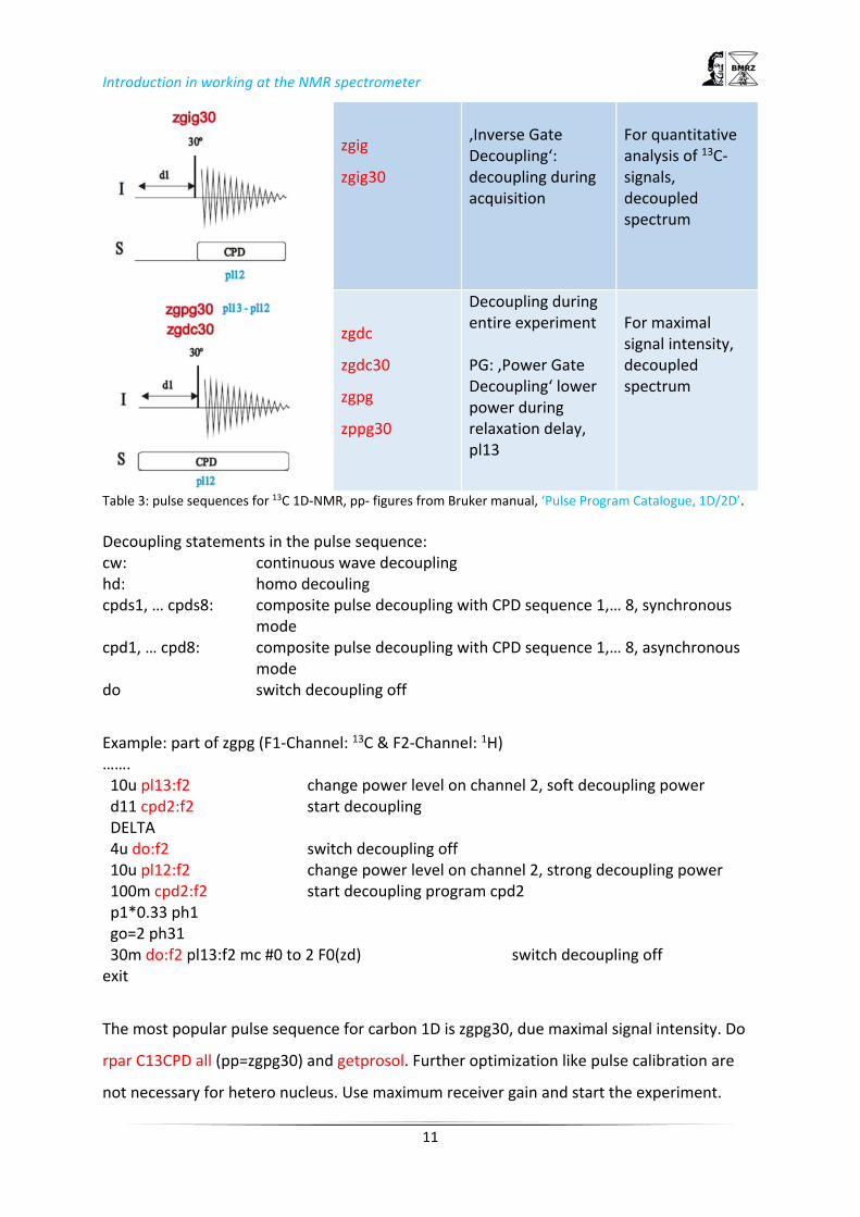
zgig

zgig30

‚Inverse Gate Decoupling‘: decoupling during acquisition

For quantitative analysis of 13C‐signals, decoupled spectrum

zgdc

zgdc30

zgpg

zppg30

Decoupling during entire experiment PG: ‚Power Gate Decoupling‘ lower power during relaxation delay, pl13

For maximal signal intensity, decoupled spectrum

Table 3: pulse sequences for 13C 1D‐NMR, pp‐ figures from Bruker manual, ‘Pulse Program Catalogue, 1D/2D’.

Decoupling statements in the pulse sequence: cw: continuous wave decoupling hd: homo decouling cpds1, … cpds8: composite pulse decoupling with CPD sequence 1,… 8, synchronous

mode cpd1, … cpd8: composite pulse decoupling with CPD sequence 1,… 8, asynchronous

mode do switch decoupling off

Example: part of zgpg (F1‐Channel: 13C & F2‐Channel: 1H) ……. 10u pl13:f2 change power level on channel 2, soft decoupling power d11 cpd2:f2 start decoupling DELTA 4u do:f2 switch decoupling off 10u pl12:f2 change power level on channel 2, strong decoupling power 100m cpd2:f2 start decoupling program cpd2 p1*0.33 ph1 go=2 ph31 30m do:f2 pl13:f2 mc #0 to 2 F0(zd) switch decoupling off exit

The most popular pulse sequence for carbon 1D is zgpg30, due maximal signal intensity. Do

rpar C13CPD all (pp=zgpg30) and getprosol. Further optimization like pulse calibration are

not necessary for hetero nucleus. Use maximum receiver gain and start the experiment.


12

Due the decoupling in a 13C 1D‐NMR the information how many protons bound to the

carbons is neglected. Polarization transfer technique like DETP bring back this information.

The DEPT starts on 1H and transfer the magnetization to 13C, which increase the sensitivity

compared to the standard 13C 1D‐NMR. DEPT Experiment can easily start by:

rpar C13DEPT135 and getprosol (or better getprosol 1H P90 PL90, if you have calibrated the

1H‐pulse). The parameter set based on the pulse sequence deptsp135, which use a adiabatic

composite pulse for refocusing. To compare how the sensitivity can profit from using adiabatic

shape in pulse sequence generate a new data set and change the pulse sequence to dept135

and re‐ measure the DEPT.

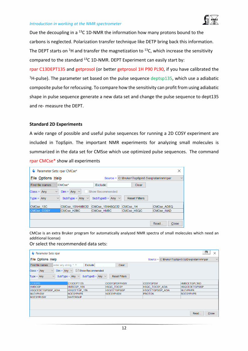
Standard 2D Experiments

A wide range of possible and useful pulse sequences for running a 2D COSY experiment are

included in TopSpin. The important NMR experiments for analyzing small molecules is

summarized in the data set for CMSse which use optimized pulse sequences. The command

rpar CMCse* show all experiments

CMCse is an extra Bruker program for automatically analyzed NMR spectra of small molecules which need an additional license)

Or select the recommended data sets:


13

2D COSY rpar CMSseCOSY

getprosol 1H P90 PL90

The parameter set based on pulse sequence cosygpmfppqf. A pulse sequence using gradient

pulses for selection with multiple quantum filter according to gradient ratio.

The sample depending parameters are acquisition time (AQ), spectral widths (SW) and

excitation frequency (o1p) should set in eda. For the indirect dimension the parameter SW1 =

SW. The minimum value for TD1, number of points in the indirect dimension should in

minimum set to 384, because the polarization transfer in COSY is happening during the t1

evolution period. That is also the reason why the receiver gain adjustment where doing in the

1H 1D‐NMR. Due the gradient selection with multiple quantum filter the experiment works

only with 1 scan.

For suppression the zero quantum coherence by the z‐filter (M.J. Thrippleton & J. Keeler,

Angew. Chem. Int. Ed. 42, 3938‐3941 (2003)) change:

pulprog cosygpphzfzs

1 FNMODE States‐TPPI

gpz0 10

NS 4

selective 1D‐NOESY experiment

Steps for setup a selective NOESY:

record a 1H 1D‐Experiment


14

select separated signals and determine the chemical shifts

generate a new dataset

rpar SELNOGP all


o1p = set to the chemical shift of the selected signal of step 2

d8 = 300ms or better the T1‐time of the selective signal of step 2

For each selected signal a new EXPERIMENT must have recorded. Be aware that the sign

between selected signals and the NOE‐signals is the opposite. Instead of using the standard

pulse sequence selnogp, use selnogpzs with better artefact suppression.

selective 1D‐TOCSY experiment

Steps for setup a selective TOCSY:

record a 1H 1D‐Experiment

select separated signals and determine the chemical shifts

generate a new dataset

rpar SELMLGP all and change pp to seldigp


o1p = set to the chemical shift of the selected signal of step 2

d9 = 20ms for only one transfer step

or set d9 = 80ms for more transfer step

For each selected signal a new EXPERIMENT must have recorded. The selected signal and the

TOCSY‐signals have the same sign. Instead of using the standard pulse sequence seldigp, use

seldigpzs with better artefact suppression.

2D HSQC / H2BC


15

Compare the different HC‐correlations:

Experiment A Experiment B Experiment C rpar HSQCETGPSI rpar CMCse_HSQC rpar C1MCseH2BC

getprosol 1H P90 PL90 AQ, o1p, SW: optimized value from the 1D

o2p 75ppm 1 SW 150ppm

1TD 64 NS 4

Compared the results, which HC correlation is the most useful experiment.

2D HMBC / sel HMBC Set up: rpar CMCse HMBC getprosol 1H P90 PL90

The pulse sequence hmbcetgpl3nd uses three‐fold low‐pass J‐filter to suppress one‐bond

correlations (D.O. Cicero, G. Barbato & R. Bazzo, J. Magn. Reson. 148, 209‐213 (2001).

AQ, o1p, SW: optimized value from the 1D o2p 100ppm 1 SW 250ppm 1TD 64 NS 8

The processing command for the HMBC is xfb and xf2m. For running a selective HMBC

change the pulse sequence to shmbcctetgpl2nd and change the recommended gradient

values. Start the shape tool (stdisp) in the 13C 1D‐data set and select a region of interest. Use

the button in shape tool to find the right pulse length for the shape

Set the pulse length (p32) and offset (spoffs32) of the shape. In a second experiment set the

offset of shape (spoffs32) to 0 and change the middle of the 13C‐frequency with smaller

spectral widths in F1. Compare all three HMBC spectra.


16

Bio‐NMR

Start a 1D 1H Experiment

WATERGATE

rpar ZGGPWG all


Pulse sequence code: zggpwg prosol relations=<triple> #include <Avance.incl> #include <Grad.incl> "p2=p1*2" "d12=20u" 1 ze 2 30m d1 10u pl1:f1 p1 ph1 50u UNBLKGRAD p16:gp1 first gradient dephases all the coherences, gpnam1=SINE.100, gpz1=20%, p16=1ms d16 pl0:f1 recovery delay, set power for F1‐Channel to pl0 (p11:sp1 ph2:r):f1 sel 90° pulse on water, p11 = 1ms, spnam1=Sinc1.1000, sp1 calculated from p1 4u d12 pl1:f1 set power back to hard power of proton pulse (p2 ph3) 4u d12 pl0:f1 (p11:sp1 ph2:r):f1 second selective 90° pulse for water, the phase 2 can be optimized in gs‐mode 46u p16: gp1 second gradient re‐phases all the resonances exceptto the on resonance solvent resonance d16 4u BLKGRAD go=2 ph31 30m mc #0 to 2 F0(zd) Exit (M. Piotto, V. Saudek, V. Sklenar, J.Biomol., 1992, 2, 661) ph1=0 2 ph2=0 0 1 1 2 2 3 3 ph3=2 2 3 3 0 0 1 1 ph31=0 2 2 0


17

Excitation Sculpting

rpar ZGESGP all


Pulse sequence code: zgesgp prosol relations=<triple> #include <Avance.incl> #include <Delay.incl> "p2=p1*2" "d12=20u" "TAU=de+p1*2/3.1416+50u" "acqt0=0" baseopt_echo

1 ze 2 30m d12 pl1:f1 BLKGRAD d1

p1 ph1 50u UNBLKGRAD p16:gp1 Start first gradient echo, p16=1ms, gpnam1=SINE.100, gpz1=31% d16 pl0:f1 recovery delay, set power for F1 to pl10=120Db

(p12:sp1 ph2:r):f1 selective 180° pulse for water, spnam1=Sinc1.100, p12=2ms, sp1 calculated from p1 4u d12 pl1:f1 set power F1 channel back to pl1

p2 ph3 non selective 180° pulse 4u p16:gp1 refocussing gradient d16 TAU p16:gp2 start second gradient echo, p16=1ms, gpnam2=SINE.100, gpz2=11% d16 pl0:f1 (p12:sp1 ph4:r):f1 selective 180° pulse for water 4u d12 pl1:f1 p2 ph5 non selective 180° pulse 4u p16:gp2 refocussing gradient d16 go=2 ph31 30m mc #0 to 2 F0(zd) 4u BLKGRAD

exit (T.‐L. Wang, A. J. Shaka, J.Mag.Res., 1995, A112) ph1=0 ph2=0 1 ph3=2 3 ph4=0 0 1 1 ph5=2 2 3 3 ph31=0 2 2 0


18

More Water suppression sequences: zggpw5, zggpjrse, Jump‐Return Echo, the best pulse sequence for analysis of RNA. zgesgppe, with perfect Echo, reduces the artifacts in 1D.

set up 2D 15N‐1H correlation, 600 MHz Setting up a 2D 15N‐1H correlation NMR experiments, like HSQC, starts with loading the Bruker

standard parameter set using the commands:

rpar <<PARAMETER SET>> getprosol 1H P90 PL90 For 15N‐ and 13C‐labeled Protein the ZGOPTNS –DLABEL_CN should be activated to enable the 13C decouplingduring the 1‐evolution period.

General starting parameters for a protein‐project at 600 MHz are:

Aq (1H) = 71ms Aq (15N) = 105ms SW (1H) = 12ppm SW (15N) = 40ppm o1p (1H) = 4.7ppm o3p (15N) = 117ppm

d (d26) = 2.631ms (cnst4 = 95 Hz) 15N dec.: pcpd3 = 220µs CPD_prog = grarp4

o2p (13C) = 101ppm 13C dec.: p14 = 500µs adiabatic pulse = Crp60,0.5.20.1 These general parameters should be optimized for each protein‐project and remembered for the 3D experiments below. In addition, check the parameters below: HSQC HMQC TROSY TROSY (sel. 15N)

Parameter set HSQCFPF3GPPHWG SFHMQCF3GPPH B_TROSYETF3GPSI B_TROSYETF3GPSI

Pulse program hsqcfpf3gpphwg sfhmqcf3gpph b_trosyetf3gpsi.2 b_trosyetf3gpsi.3

DS 32 32 32 32

NS 8 32 32 32

d1 [s] 1 0.2 0.2 0.2 1H selective pulses

sp1 (90°pulse) Sinc1.1000 p11 1 ms

sp23 (120°pulse) Pc9_4_120.1000 p39 2.4 ms

sp26 (180°pulse) Repurp.1000 p42 1.4 ms

sp25 (90°pulse) Pc9_4_90.1000 p41 2.2 ms

sp24 (180°pulse) Rsnob.1000 p40 0.8 ms

sp28 (90°pulse) Eburp2.1000 p43 1.7 ms

sp26 (180°pulse) Repurp.1000 p42 1.4 ms

sp29 (90°pulse) Eburp2tr.1000 p43 1.7 ms

sp28 (90°pulse) Eburp2.1000 p43 1.7 ms

sp29 (90°pulse) Eburp2tr.1000 p43 1.7 ms

15N selective pulses

sp39 (180°pulse) Reburp.1000 p56 1.6 ms


19

sp40 (180°pulse) Bip720,50,20.1 p56 0.5 msA

Table2: Parameters for 2D 15N‐1H correlation experiments. A 500 µs at all field strength

New option in Topspin 3.5: Setting ZGOPTNS to ‐DCALC_SP (or ‐DCALC_SP ‐DLABEL_CN for 13C

& 15N labeled proteins) allows to automatically calculate all the band‐selective proton pulses, based

on cnst54 and cnst55 and the manually determined p1

cnst54: H(N) chemical shift (offset, in ppm), Protein: 8.5 RNA: 12.3 cnst55: H(N) bandwidth (in ppm), for both 4.8

Shape pulses

Calculation of radiofrequency field strength B1

The magnetization vector precesses around the radiofrequency field B1 according to

(1)

The angle precession q (in rad), is proportional to the pulse width p:

(2)

For a 90° pulse () and Equation (1): (3)

Types of shape pulses 90° pulses (excitation, Iz Iy) 180° pulses

o Inversion pulses, Iz ‐Iz o Refocusing pulses, Iy ‐Iy

Very narrow excitation o Solvent suppression (e.g. Sinc, Gauss, Square pulses)

Excitation / Inversion of a region Ca, C’… o Gaussian Cascades

180° pulses: Q3, G3 90° pulses: Q5, Q5tr, G4, G4tr

Broadband Inversion/ Refocusing o Inversion, Iz ‐Iz

Adiabatic pulses (e.g. smoothed Chirp pulses) Broadband Inversion pulses (BIPs)

o Refocusing, Ix ‐Ix or Iy ‐Iy Composite adiabatic pulses (e.g. Composite Chirp)

Nomenclature for shapes in Topspin:

Standard shapes, e.g. Q5tr.1000 o Shape (Q5 time reversed) o Number of points (1000)

Adiabatic shapes, e.g. Crp60, 05,20.1


20

o Shape and sweep width (Chirp, 60 kHz) o duration (0.5 ms) o Smoothing and number of points (20% and 1000)

Instead of using band‐selective pulses, for protein NMR selective rectangular pulses can be

applied due the large chemical shift difference between CO and CA. The excitation profile with

maximum on CA and minimum on CO is calculated as follows:

Both equations can be implemented in a pulse sequence using cnst21 (CO chemical shift) and cnst22 (CA chemical shift) with the following definitions:

90°‐pulse: "pxx=3.873*1000000/((cnst21‐cnst22)*bf2*4)" 180° ‐pulse "pxx=1.732*1000000/((cnst21‐cnst22)*bf2*2)"

Setup 3D Experiment First read a standard parameter set, e.g. for the protein backbone 3D experiments

rpar <<PARAMETER SET>> getprosol 1H P90 PL90 set the optimized general parameters from the HSQC

protein backbone 3D experiments based on WATERGATE: HNCOGPWG3D, HNCACOGPWG3D, HNCAGPWG3D, HNCOCAGPWG3D, HNCACBGPWG3D, HNCOCACBGPWG3D

protein backbone 3D experiments based on Best‐method: B_HNCOGP3D, B_HNCACOGP3D, B_HNCAGP3D, B_HNCOCAGP3D; B_HNCACBGP3D, B_HNCOCACBGP3D

protein backbone 3D experiments based on Best‐TROSY‐Method: B_TRHNCOGP3D, B_TRHNCACOGP3D, B_TRHNCAGP3D, B_TRHNCOCAGP3D; B_TRHNCACBGP3D, B_TRHNCOCACBGP3D

Which 3D methods is the best option for protein assignment depends on the size of the

molecule. This can be experimentally tested by recording the carbon plane in a 3D HNCO. This


21

can be done by setting the number of points in the evolution period of 15N (F2) to 1 and 13C(F3)

to 128, td.

Processing the 2D Plane in a 3D dataset.

Checking reverse statement during transformation: reverse

Depends on the pulse sequence, hncogpwg3d: FALSE; b_hncogp3d.2 & b_trhncogp3d.2:

TRUE 2D processing command FT: xfb

o Enter a new PROCNO for 2D data: e.g. 13 (store the carbon‐plane in procno 13 and 15N plane in procno 23).

2D processing command for phase correction: apk2d Compare the 2D spectra:

o read out the 1D projection, by rhpp 2 (read horizontal positive projection and store it in procno 2)

Additional Information All implemented NMR‐experiments in TopSpin are described in the manual ‘pulse program

catalogue BIO’.

In TopSpin a wide range of NMR experiments are implemented as parameter set which can

easily use. A selection of important experiments follows below:

Parameter sets for protein experiment with best method: rpar B_*


22

Parameter sets for 4 dimensional NMR experiments: rpar *4D*

Parameter sets for 13C direct detection: rpar C_*

Parameter sets for nucleic acids: rpar NA_*


23

NUS – Non Uniform Sampling

The general concept of NUS is summarized in TopSpin manual ‘NUS Parameters’. The NUS

reduced for a multidimensional NMR‐experiment the number of points for the indirect

dimension by using algorithm. For using NUS in setup NMR‐Experiments only minor changes

of the parameter setup are necessary. First, you set up the 2D, 3D or 4D NMR experiments in

the described way before. The NUS will be activated for the data set by selecting the

parameter FnTYPE as non‐uniform_ sampling in eda.

In the category NUS of eda the number NusAMOUNT [%] selected how many total points are

recorded for the indirect dimension.

The choice of NusAMOUNT [%] compromised between as less as possible points and getting

a multidimensional NMR spectrum without artefacts. From practical experiences is used as

recommended values 50% for 2D NMR and 25% for 3D & 4D NMR. The parameter NusT2 [sec]

weight the calculated points combination for the indirect dimension. If all NusT2 1 yields in

equal distribution of all points. For protein NMR experiment the suggestion of NusT2:

1H(aliphatic):0.02 15N: 0.05 13C: 0.5,

which weight the points distribution more to beginning of the experiment, shown by press

Show button. Result:


24

Processing of NUS data. TopSpin recognized automatic if the date were recorded with NUS and do the processing like

usually. For processing of NUS data two algorithm are implemented in TopSpin: MDD and CS.

Both need an additional license for processing, but not for recording the data. Which

algorithm are used can define by the parameter Mdd_mod in edp, showing below:

General, in the most cases the CS algorithm give a better result, but the processing takes

longer. For that reason, optimized the other processing parameter with MDD and select CS

for final processing. In TopSpin 3.5 the CS algorithm is included for free by processing 2D data.

.

Exercise at the...

Documents

Transcript of Exercise at the...