Exercise 4. Single-Species, Single-Season Occupancy with ... · sampled. In the next exercise, we...
129
Exercises in Occupancy Estimation and Modeling; Donovan and Hines 2007 Chapter 4 Page 1 6/15/2007 EXERCISE 4: SINGLE-SPECIES, SINGLE-SEASON MODEL WITH SITE LEVEL COVARIATES Please cite this work as: Donovan, T. M. and J. Hines. 2007. Exercises in occupancy modeling and estimation. <http://www.uvm.edu/envnr/vtcfwru/spreadsheets/occupancy/occupancy.htm >
Transcript of Exercise 4. Single-Species, Single-Season Occupancy with ... · sampled. In the next exercise, we...

Exercises in Occupancy Estimation and Modeling; Donovan and Hines 2007
Chapter 4 Page 1 6/15/2007
EXERCISE 4: SINGLE-SPECIES, SINGLE-SEASON MODEL WITH SITE
LEVEL COVARIATES
Please cite this work as: Donovan, T. M. and J. Hines. 2007. Exercises in
occupancy modeling and estimation.
<http://www.uvm.edu/envnr/vtcfwru/spreadsheets/occupancy/occupancy.htm>
Exercises in Occupancy Estimation and Modeling; Donovan and Hines 2007
Chapter 4 Page 2 6/15/2007
TABLE OF CONTENTS
SINGLE-SPECIES, SINGLE-SEASON MODEL WITH SITE LEVEL COVARIATES SPREADSHEET EXERCISE ....................................................................4
OBJECTIVES............................................................... 4 BACKGROUND.............................................................. 4 EXAMPLES OF LINEAR COVARIATE MODELS.......................... 5 SAMPLING DESIGN ....................................................... 8 SPREADSHEET SET-UP ................................................... 9 DETECTION PROBABILITY ..............................................10 SITE LEVEL COVARIATES...............................................11 STANDARDIZED COVARIATE VALUES.................................12 CODING TREATMENTS ..................................................15 USING LINEAR MODELS TO ESTIMATE SITE-SPECIFIC PSI......16 LN(ODDS) OR LOGIT MODELS..........................................17 THE LOGIT LINK.........................................................19 POLYNOMIAL LINEAR MODELS ........................................22 CATEGORICAL LINEAR MODELS .......................................24 ADDITIVE LINEAR MODELS ............................................26 LINEAR MODELS WITH INTERACTIVE EFFECTS ....................30 MODELING LOGIT EQUATIONS IN THE SPREADSHEET............31 MISSING COVARIATE VALUES.........................................33 MODEL P(.)PSI(.) .........................................................34 MODEL P(.)PSI(Patch Size) ..............................................35 PROBABILITY OF GETTING A PARTICULAR ENCOUNTER HISTORY37 THE MULTINOMIAL LOG LIKELIHOOD FOR INDIVIDUAL COVARIATE MODELS ...................................................................39 MAXIMIZING THE LN LIKELIHOOD...................................39 INTERPRETING THE MODEL OUTPUT .................................40 TRACKING RESULTS .....................................................44 MODEL P(.)PSI(Patch Size + Patch Size2) ..............................45 MODEL P(.)PSI(habitat) ..................................................47 Model P(.)PSI(Patch Size + Habitat) ....................................49 Model P(.)PSI(Patch Size * Habitat) ....................................50 COMPARING MODELS....................................................51 MODEL AVERAGING AND MULTI-MODEL INFERENCE ..............55 ASSESSING MODEL FIT ................................................56 THE MacKENZIE BAILEY GOODNESS OF FIT TEST .................57 THE BOOTSTRAP.........................................................60
Exercises in Occupancy Estimation and Modeling; Donovan and Hines 2007
Chapter 4 Page 3 6/15/2007
SIMULATING COVARIATE DATA.......................................70 CREATING INPUT FILES FOR MARK AND PRESENCE................73
SINGLE-SPECIES, SINGLE-SEASON OCCUPANCY WITH SITE COVARIATES IN PROGRAM PRESENCE.................................................................................... 74
INPUT DATA..............................................................74 MODEL P(.)PSI(Patch Size) ..............................................78 ASSESSING MODEL FIT ................................................91 MODEL P(.)PSI(PATCH SIZE + PATCH SIZE2) ........................93 MODEL P(.)PSI(HABITAT) ...............................................97 MODEL P(.)PSI(PATCH SIZE + HABITAT) ........................... 100 MODEL P(.)PSI(HABITAT * PATCH SIZE) ........................... 103
INTERPRETING THE RESULTS BROWSER: MODEL SELECTION METHODS........................................................................... 105 INPUT DATA............................................................ 107 GETTING STARTED .................................................... 107 MARK PIMS ............................................................. 109 MODEL P(.)PSI(PATCH SIZE) ......................................... 111 MODEL P(Date)PSI(Patch Size) OUTPUT ............................. 117 MODEL P(Date + Rain) PSI(Habitat) .................................. 123 MODEL P(Date+Temp+Rain)PSI(Patch Size + Habitat)............... 126 MODEL AVERAGING.................................................... 129
Exercises in Occupancy Estimation and Modeling; Donovan and Hines 2007
Chapter 4 Page 4 6/15/2007
SINGLE-SPECIES, SINGLE-SEASON MODEL WITH SITE LEVEL COVARIATES SPREADSHEET EXERCISE
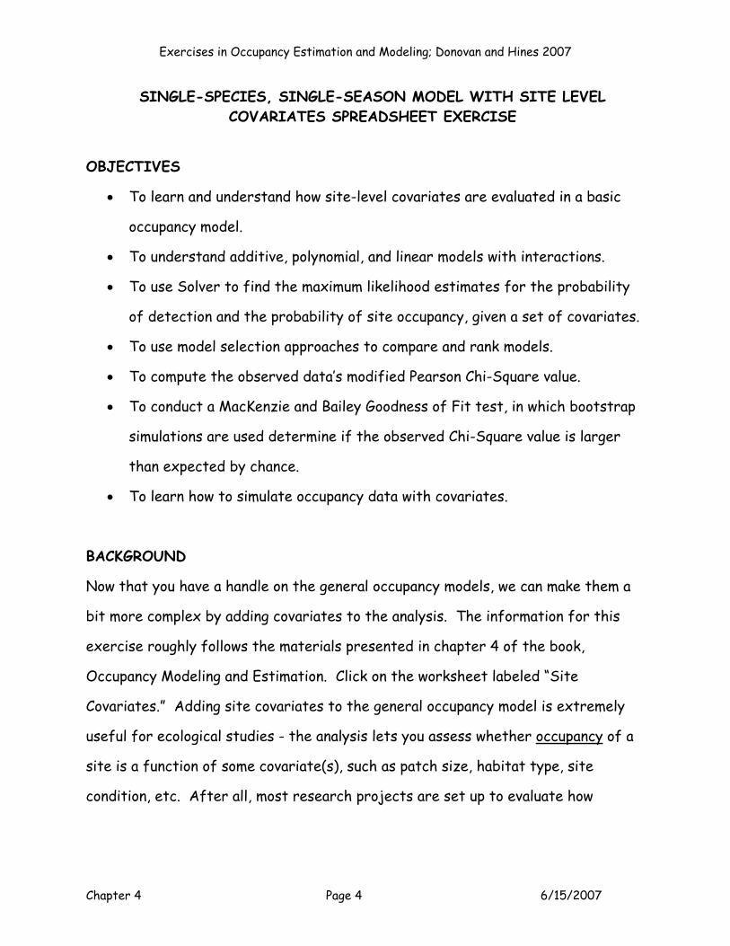
OBJECTIVES
• To learn and understand how site-level covariates are evaluated in a basic
occupancy model.
• To understand additive, polynomial, and linear models with interactions.
• To use Solver to find the maximum likelihood estimates for the probability
of detection and the probability of site occupancy, given a set of covariates.
• To use model selection approaches to compare and rank models.
• To compute the observed data’s modified Pearson Chi-Square value.
• To conduct a MacKenzie and Bailey Goodness of Fit test, in which bootstrap
simulations are used determine if the observed Chi-Square value is larger
than expected by chance.
• To learn how to simulate occupancy data with covariates.
BACKGROUND
Now that you have a handle on the general occupancy models, we can make them a
bit more complex by adding covariates to the analysis. The information for this
exercise roughly follows the materials presented in chapter 4 of the book,
Occupancy Modeling and Estimation. Click on the worksheet labeled “Site
Covariates.” Adding site covariates to the general occupancy model is extremely
useful for ecological studies - the analysis lets you assess whether occupancy of a
site is a function of some covariate(s), such as patch size, habitat type, site
condition, etc. After all, most research projects are set up to evaluate how
Exercises in Occupancy Estimation and Modeling; Donovan and Hines 2007
Chapter 4 Page 5 6/15/2007
covariates affect occupancy probability, so you might as well learn how to analyze
covariates correctly!
Let’s step back for a second and answer the question, “what exactly is meant by a
“covariate” effect?” Well, remember the parameters of the “general” occupancy
model we analyzed in the previous exercise: p1, p2, p3, and ψ. The only raw data we
had to run a model were the encounter history frequencies. We found the
combination of parameter estimates that maximized the multinomial log likelihood.
But with covariate analyses, a lot of other data is collected at a site in addition to
the encounter history frequencies. For example, you might collect data on the
date the site was sampled, the time the site was sampled, weather conditions of
the sampling period, as well as physical and biological characteristics of the site.
The data can be collected remotely (with GIS) as well as on-site. The covariates
you collect could help explain differences in ψ among the sites (site-level
covariates) or could help explain differences in detection probabilities among the
surveys (survey-specific covariates). In this exercise, we will focus on site-level
covariates that explain differences in occupancy probability among the sites
sampled. In the next exercise, we will focus on survey-specific covariates that
explain differences in detection probability among the different replicate samples.
EXAMPLES OF LINEAR COVARIATE MODELS
Our focus will be on two covariates that might influence the probability that a
given site is occupied: patch size and habitat type. To begin, suppose you think
that “patch size” could affect the probability that a site is occupied. In this case,
the patch size is called a “site” covariate because whether a site is occupied or not
is a function of the individual site’s patch size. In this example, patch size is a

Exercises in Occupancy Estimation and Modeling; Donovan and Hines 2007
Chapter 4 Page 6 6/15/2007
continuous covariate, where the values fall within a given range (e.g., 1 ha to 1000
ha patches). Because each site has its own patch size, each site will end up with a
unique probability of occupancy that is directly linked to its corresponding patch
size. As a second example, suppose that whether a site is occupied or not depends
on the habitat type associated with that site. In this case, habitat type is a site-
level covariate that is categorical. A categorical variable can take on one of many
discrete values; e.g., a person’s eye color can be blue, brown, green, or hazel.
Habitat type is another is another example of a categorical variable, where values
can be “grassland,” “forest,” and “wetland.” A site is characterized as one of these
types only; i.e., a site can’t be characterized as both grassland and wetland.
One important point to keep in mind is that, for a single season occupancy model,
the sites are assumed to be closed – meaning that the occupancy status of the site
cannot change over the course of sampling periods. As such, it makes sense that
covariates thought to affect occupancy are relatively stable (or unchanging) over
the season. Covariates such as patch size work well in this context because patch
size will not likely change within a single season. However, covariates such as
temperature or date make less sense because these values can change within a
sampling season.
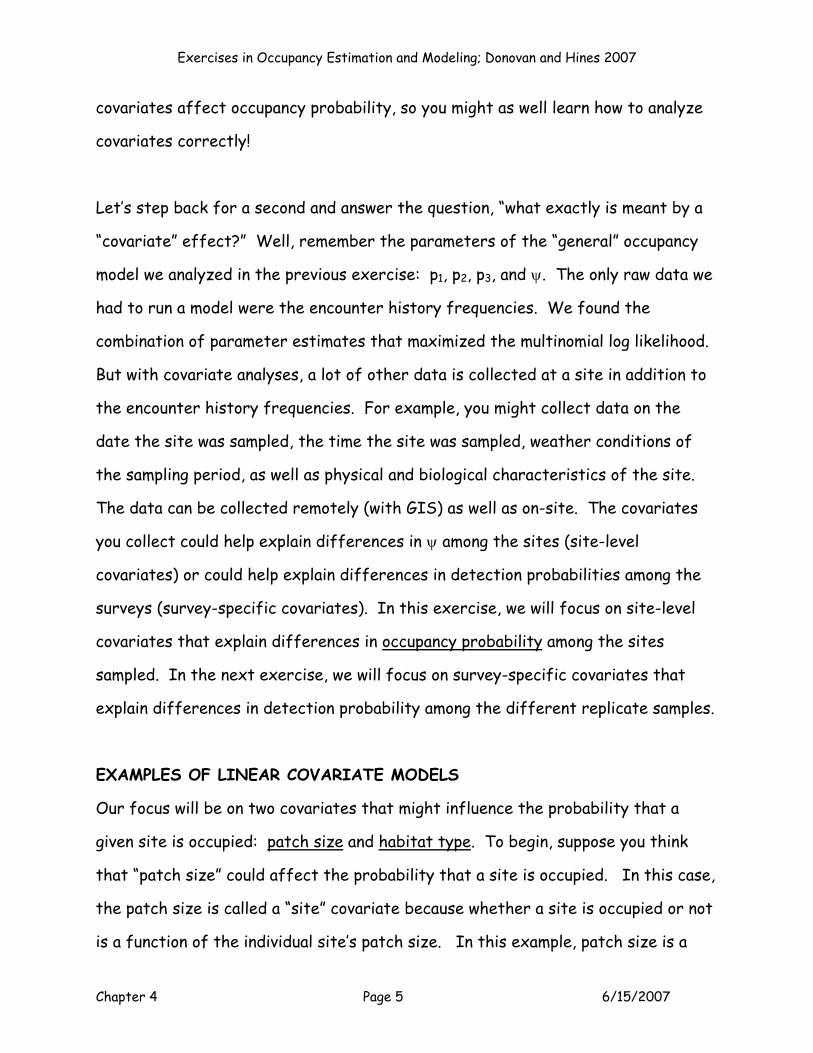
Here’s what you can look forward to in this exercise -- we’ll be exploring five
different linear models where psi is a function of covariates:
1. Psi is a linear function of patch size:
Exercises in Occupancy Estimation and Modeling; Donovan and Hines 2007
Chapter 4 Page 7 6/15/2007
0
0.1
0.2
0.3
0.4
0.5
0.6
0.7
0.8
0.9
1
-4 -3 -2 -1 0 1 2 3 4
Patch Size
Psi
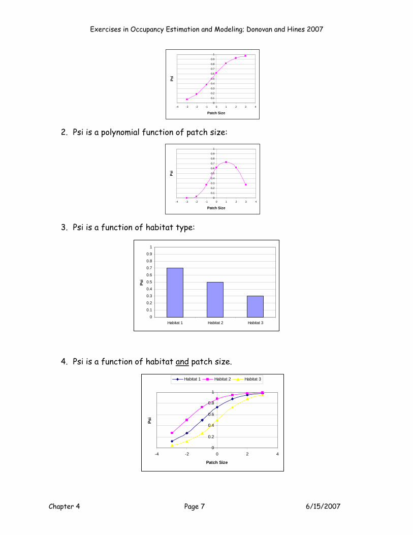
2. Psi is a polynomial function of patch size:
0
0.1
0.2
0.3
0.4
0.5
0.6
0.7
0.8
0.9
1
-4 -3 -2 -1 0 1 2 3 4
Patch Size
Psi
3. Psi is a function of habitat type:
0
0.1
0.2
0.3
0.4
0.5
0.6
0.7
0.8
0.9
1
Habitat 1 Habitat 2 Habitat 3
Psi
4. Psi is a function of habitat and patch size.
0
0.2
0.4
0.6
0.8
1
-4 -2 0 2 4
Patch Size
Psi
Habitat 1 Habitat 2 Habitat 3

Exercises in Occupancy Estimation and Modeling; Donovan and Hines 2007
Chapter 4 Page 8 6/15/2007
5. Psi is a function of an interaction between habitat and patch size.
-0.2
0
0.2
0.4
0.6
0.8
1
-4 -2 0 2 4
Patch Size
Psi
Habitat 1 Habitat 2 Habitat 3
All of these are examples of linear models in the statistical sense (even though the
graphs don’t look linear!). Psi might be also be a function of many other physical or
biological properties of the site, such as food levels, number of predators, distance
to other patches, etc. However, we will cover a LOT of ground (a crash course in
linear modeling, in fact) just by focusing on the 5 linear models that include patch
size (which is continuous), habitat (which is categorical), and combinations of patch
size and habitat. Then, we’ll use model selection procedures to compare the five
different models. Finally, we’ll run a parametric bootstrap to assure that at least
one model in our model set “fits” the underlying occupancy model to an acceptable
degree. This is a long exercise (sorry about that!), so let’s get started.
SAMPLING DESIGN
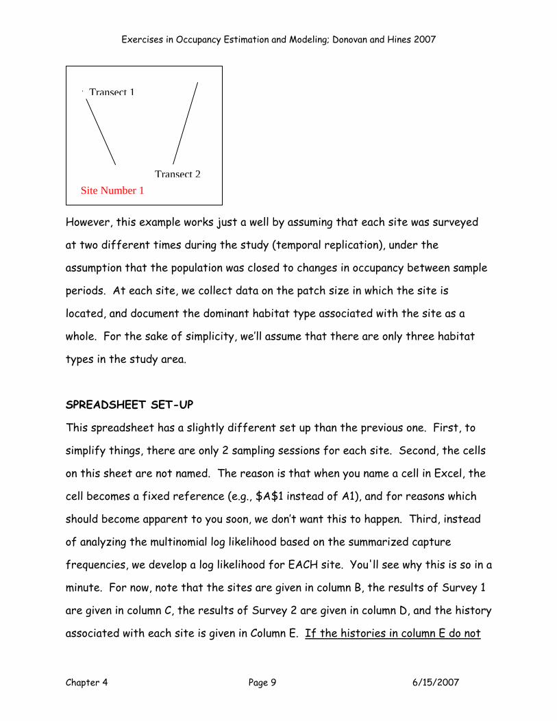
In this spreadsheet, we’ll assume that each site is surveyed by searching for the
target species along two, spatially replicated transects (each sample was conducted
in a different location within the site).
Exercises in Occupancy Estimation and Modeling; Donovan and Hines 2007
Chapter 4 Page 9 6/15/2007
However, this example works just a well by assuming that each site was surveyed
at two different times during the study (temporal replication), under the
assumption that the population was closed to changes in occupancy between sample
periods. At each site, we collect data on the patch size in which the site is
located, and document the dominant habitat type associated with the site as a
whole. For the sake of simplicity, we’ll assume that there are only three habitat
types in the study area.
SPREADSHEET SET-UP
This spreadsheet has a slightly different set up than the previous one. First, to
simplify things, there are only 2 sampling sessions for each site. Second, the cells
on this sheet are not named. The reason is that when you name a cell in Excel, the
cell becomes a fixed reference (e.g., $A$1 instead of A1), and for reasons which
should become apparent to you soon, we don’t want this to happen. Third, instead
of analyzing the multinomial log likelihood based on the summarized capture
frequencies, we develop a log likelihood for EACH site. You'll see why this is so in a
minute. For now, note that the sites are given in column B, the results of Survey 1
are given in column C, the results of Survey 2 are given in column D, and the history
associated with each site is given in Column E. If the histories in column E do not
Transect 1
Transect 2Site Number 1
Exercises in Occupancy Estimation and Modeling; Donovan and Hines 2007
Chapter 4 Page 10 6/15/2007
match the histories in column A, please copy the values from A16:A215 to E16:215
to restore the original site history values so that your analysis matches the
exercise values.
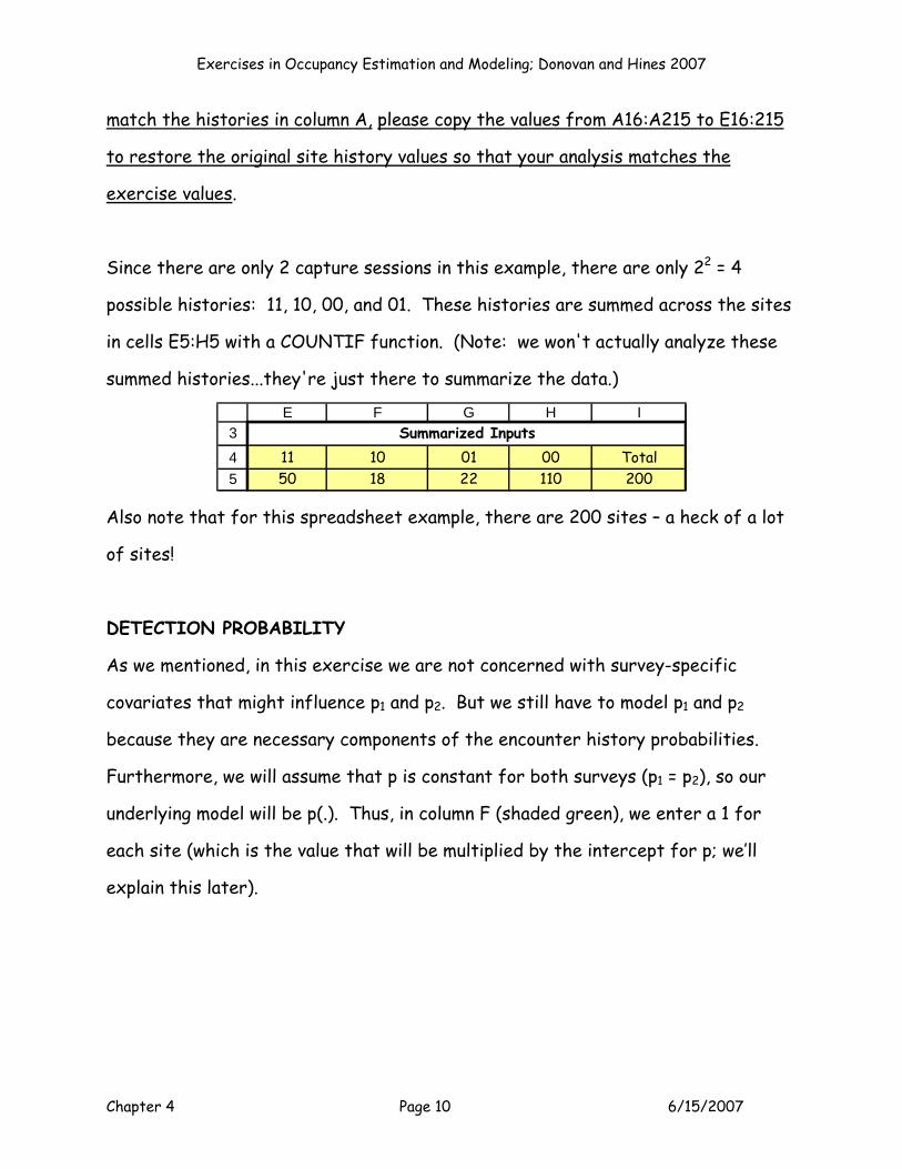
Since there are only 2 capture sessions in this example, there are only 22 = 4
possible histories: 11, 10, 00, and 01. These histories are summed across the sites
in cells E5:H5 with a COUNTIF function. (Note: we won't actually analyze these
summed histories...they're just there to summarize the data.)
3
45
E F G H I
11 10 01 00 Total50 18 22 110 200
Summarized Inputs
Also note that for this spreadsheet example, there are 200 sites – a heck of a lot
of sites!
DETECTION PROBABILITY
As we mentioned, in this exercise we are not concerned with survey-specific
covariates that might influence p1 and p2. But we still have to model p1 and p2
because they are necessary components of the encounter history probabilities.
Furthermore, we will assume that p is constant for both surveys (p1 = p2), so our
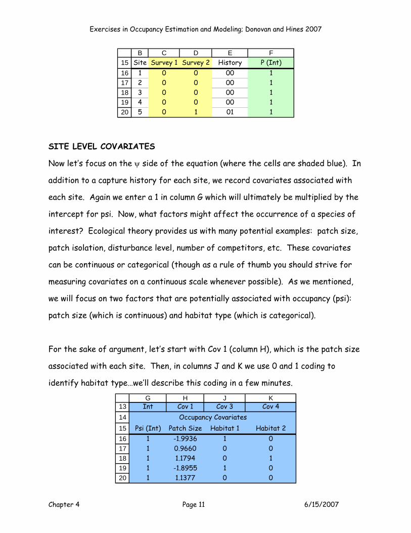
underlying model will be p(.). Thus, in column F (shaded green), we enter a 1 for
each site (which is the value that will be multiplied by the intercept for p; we’ll
explain this later).
Exercises in Occupancy Estimation and Modeling; Donovan and Hines 2007
Chapter 4 Page 11 6/15/2007
151617181920
B C D E FSite Survey 1 Survey 2 History P (Int)
1 0 0 00 12 0 0 00 13 0 0 00 14 0 0 00 15 0 1 01 1
SITE LEVEL COVARIATES
Now let’s focus on the ψ side of the equation (where the cells are shaded blue). In
addition to a capture history for each site, we record covariates associated with
each site. Again we enter a 1 in column G which will ultimately be multiplied by the
intercept for psi. Now, what factors might affect the occurrence of a species of
interest? Ecological theory provides us with many potential examples: patch size,
patch isolation, disturbance level, number of competitors, etc. These covariates
can be continuous or categorical (though as a rule of thumb you should strive for
measuring covariates on a continuous scale whenever possible). As we mentioned,
we will focus on two factors that are potentially associated with occupancy (psi):
patch size (which is continuous) and habitat type (which is categorical).
For the sake of argument, let’s start with Cov 1 (column H), which is the patch size
associated with each site. Then, in columns J and K we use 0 and 1 coding to
identify habitat type…we’ll describe this coding in a few minutes.
1314151617181920
G H J KInt Cov 1 Cov 3 Cov 4
Psi (Int) Patch Size Habitat 1 Habitat 21 -1.9936 1 01 0.9660 0 01 1.1794 0 11 -1.8955 1 01 1.1377 0 0
Occupancy Covariates
Exercises in Occupancy Estimation and Modeling; Donovan and Hines 2007
Chapter 4 Page 12 6/15/2007
STANDARDIZED COVARIATE VALUES
Now that we know what the potential covariates are (patch size and habitat), let’s
look at the values that are entered for the first 5 sites (above). You should notice
first off that the categorical covariates (habitat: Cov 3, 4) contain only 0’s and 1’s,
whereas the continuous covariates (patch size: Cov 1) range from about +3 to -3.
For example, site 1 had a patch size covariate of -1.9936; site 2 had a patch size
covariate of 0.9660, and site 4 had a patch size covariate of -1.8955. But you
might be scratching your head and thinking, “How can patch size have a value of -
1.8955?” The answer is that the continuous variables have been standardized.
That is, they’ve been converted to Z scores. You might remember from your
introductory stats course that the Z transformation takes continuous data, and
standardizes the data so that the mean for the population is 0 and the standard
deviation is 1. This is done by computing the mean and the standard deviation for
the raw data; each raw covariate score is then standardized by subtracting the
mean from raw value, and then dividing the result by the standard deviation:
Z = (raw score – mean score)/standard deviation.
If you have raw data, you can convert them to Z scores with the STANDARDIZE
spreadsheet function. Z values range from about +3 to -3, and a 0 indicates the
average. About 68% of the Z data should have values between +1 and -1, and about
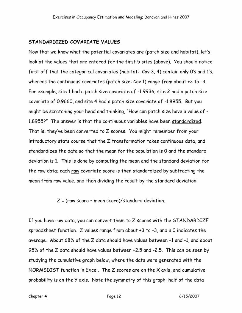
95% of the Z data should have values between +2.5 and -2.5. This can be seen by
studying the cumulative graph below, where the data were generated with the
NORMSDIST function in Excel. The Z scores are on the X axis, and cumulative
probability is on the Y axis. Note the symmetry of this graph: half of the data
Exercises in Occupancy Estimation and Modeling; Donovan and Hines 2007
Chapter 4 Page 13 6/15/2007
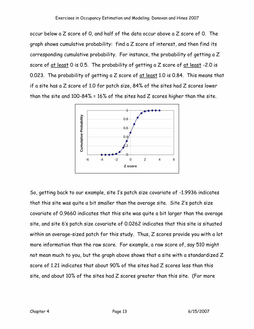
occur below a Z score of 0, and half of the data occur above a Z score of 0. The
graph shows cumulative probability: find a Z score of interest, and then find its
corresponding cumulative probability. For instance, the probability of getting a Z
score of at least 0 is 0.5. The probability of getting a Z score of at least -2.0 is
0.023. The probability of getting a Z score of at least 1.0 is 0.84. This means that
if a site has a Z score of 1.0 for patch size, 84% of the sites had Z scores lower
than the site and 100-84% = 16% of the sites had Z scores higher than the site.
0
0.2
0.4
0.6
0.8
1
-6 -4 -2 0 2 4 6
Z score
Cum
ulat
ive
Prob
abili
ty
So, getting back to our example, site 1’s patch size covariate of -1.9936 indicates
that this site was quite a bit smaller than the average site. Site 2’s patch size
covariate of 0.9660 indicates that this site was quite a bit larger than the average
site, and site 6’s patch size covariate of 0.0262 indicates that this site is situated
within an average-sized patch for this study. Thus, Z scores provide you with a lot
more information than the raw score. For example, a raw score of, say 510 might
not mean much to you, but the graph above shows that a site with a standardized Z
score of 1.21 indicates that about 90% of the sites had Z scores less than this
site, and about 10% of the sites had Z scores greater than this site. (For more
Exercises in Occupancy Estimation and Modeling; Donovan and Hines 2007
Chapter 4 Page 14 6/15/2007
information on Z scores, see http://www-
stat.stanford.edu/~naras/jsm/FindProbability.html).
Why standardize? The major reason is provided by Gary White in the MARK
helpfiles: “When the mean value of individual covariates is very large or small, or
the range of the covariate is over several orders of magnitude, the numerical
optimization algorithm may fail to find the correct parameter estimates.” Aside
from converting your raw data to Z scores, there are other ways to avoid this
problem. For instance, if you are dealing with temperature or elevation data, you
could simply divide the raw scores by some constant to reduce the range of the
data itself. Here is a quote from the Program PRESENCE page about
strandardizing/transforming covariates: “The best approach is to transform your
data onto another scale which is still meaningful to you. You could divide the
covariate values by some constant (i.e., rather than entering 80% humidity as 80.0,
use 0.80); subtract the average of the covariates from each observed value (i.e.,
X* = X – average(X’s)); or some combination of the two. Such transformations are
not carried out by PRESENCE automatically, but can be done easily with a
spreadsheet and the modified values pasted back into the Data Window.”
Gary provides a warning about the use of Z scores in the MARK helpfiles:
“One caution is in order about using the z transformation on one or more individual
covariates and another temporal or group covariate in the design matrix to predict
a single real parameter. Situations can arise where the real parameter estimates
and the model's AIC differ between runs using the standardized covariates and
the unstandardized covariates. This situation arises because the z transformation
Exercises in Occupancy Estimation and Modeling; Donovan and Hines 2007
Chapter 4 Page 15 6/15/2007
affects both the slope and intercept of the model.” There is a very good
description of this problem in Chapter 12 of Cooch and White’s book, “MARK: A
Gentle Introduction.”
CODING TREATMENTS
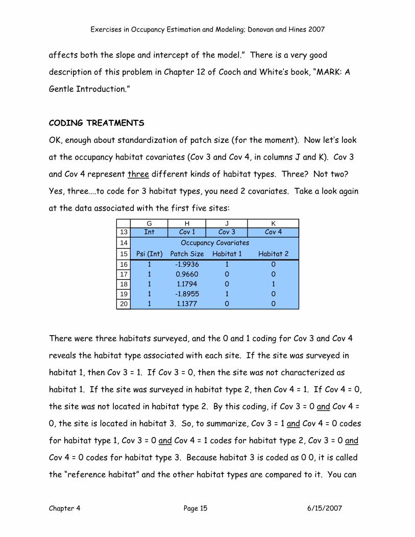
OK, enough about standardization of patch size (for the moment). Now let’s look
at the occupancy habitat covariates (Cov 3 and Cov 4, in columns J and K). Cov 3
and Cov 4 represent three different kinds of habitat types. Three? Not two?
Yes, three….to code for 3 habitat types, you need 2 covariates. Take a look again
at the data associated with the first five sites:
1314151617181920
G H J KInt Cov 1 Cov 3 Cov 4
Psi (Int) Patch Size Habitat 1 Habitat 21 -1.9936 1 01 0.9660 0 01 1.1794 0 11 -1.8955 1 01 1.1377 0 0
Occupancy Covariates
There were three habitats surveyed, and the 0 and 1 coding for Cov 3 and Cov 4
reveals the habitat type associated with each site. If the site was surveyed in
habitat 1, then Cov 3 = 1. If Cov 3 = 0, then the site was not characterized as
habitat 1. If the site was surveyed in habitat type 2, then Cov 4 = 1. If Cov 4 = 0,
the site was not located in habitat type 2. By this coding, if Cov 3 = 0 and Cov 4 =
0, the site is located in habitat 3. So, to summarize, Cov 3 = 1 and Cov 4 = 0 codes
for habitat type 1, Cov 3 = 0 and Cov 4 = 1 codes for habitat type 2, Cov 3 = 0 and
Cov 4 = 0 codes for habitat type 3. Because habitat 3 is coded as 0 0, it is called
the “reference habitat” and the other habitat types are compared to it. You can

Exercises in Occupancy Estimation and Modeling; Donovan and Hines 2007
Chapter 4 Page 16 6/15/2007
make the reference habitat any type you want (1, 2, or 3) by altering your coding
system. You might be wondering, “what if Cov 3 = 1 and Cov 4 = 1? What does that
code for?” The answer is it’s not a valid coding for habitat type (in this case)
because it suggests the site is both habitat 1 and habitat 2. Using this coding
system, sites 1 and 4 were in habitat 1, sites 3 was in habitat 2, and sites 2 and 5
were in habitat 3. We’ll come back to this in a bit. For now all you need to
understand is that each site has its own history and its own set of covariates, how
continuous covariates are standardized, and how categorical covariates are coded.
You’ve probably noticed that there are three other covariates in the dataset (Cov
2, Cov 5 and Cov 6). These covariates are computed from the patch size and
habitat covariates. For example, Cov 2 is patch size squared, so the formula in cell
I16 is =H16^2. We will visit this covariate when we run a polynomial model.
Similarly, Cov 5 and Cov 6 are computed by multiplying patch size by the habitat
coding. We will visit these covariates when we run the patch size by habitat
interaction model. Thus, we have 6 site-level covariates available for modeling.
1314151617181920
G H I J K L MInt Cov 1 Cov 2 Cov 3 Cov 4 Cov 5 Cov 6
Psi (Int) Patch Size Patch Size 2 Habitat 1 Habitat 2 H1*PS H2*PS1 -1.9936 3.9743 1 0 -1.994 0.0001 0.9660 0.9332 0 0 0.000 0.0001 1.1794 1.3911 0 1 0.000 1.1791 -1.8955 3.5929 1 0 -1.895 0.0001 1.1377 1.2943 0 0 0.000 0.000
Occupancy Covariates
USING LINEAR MODELS TO ESTIMATE SITE-SPECIFIC PSI
OK, now given each site's covariate values, we need to determine what p and ψ are
for each site. (Remember that our underlying model is p(.)psi(covariate), so we are
Exercises in Occupancy Estimation and Modeling; Donovan and Hines 2007
Chapter 4 Page 17 6/15/2007
interested in estimating two real parameters, p and psi, and we’ll do this on a site-
by-site basis). Let’s focus on only one covariate (patch size) to begin with….we’ll
add more covariates after you have a handle on the basics. Let’s assume that as
the standardized Z score for patch size increases or decreases, the probability of
occupancy increases or decreases in a predictable fashion. We could use a
regression model to do this:
psi = B0 + B1 * covariate, or in our case…
psi = B0 + B1 * standardized patch size.
OK, if you’ve taken an introductory stats course you’ll notice that this is the
equation of a line (y = mx+b, or y = B0 + B1x) and by knowing B0 (the intercept) and
B1 (the slope), as well as a site’s Z score for patch size, you can estimate psi with
linear regression approaches. If B1 is positive, the relationship is positive, where
sites with high Z scores (i.e., those sites with larger patch sizes) will have a higher
occupancy probability, and if B1 is negative, the relationship is a negative
relationship where sites with high Z scores will have a lower occupancy probability.
LN(ODDS) OR LOGIT MODELS
But, hang on! Psi is a probability, and is bounded between 0 and 1. We can’t do a
regression analysis for this model because regression analysis requires that the
response variable (psi) be unbounded. What now? The way around this problem
involves converting the probability, psi, to odds, and then taking the natural log of
the odds, and then modeling the log odds (or logit) of psi instead of psi, and then
back-transforming the logit of psi to get psi. Hmmmm, let’s try that more slowly.
You’re all familiar with odds (e.g., “what are the odds that the Chicago Cubs will win
Exercises in Occupancy Estimation and Modeling; Donovan and Hines 2007
Chapter 4 Page 18 6/15/2007
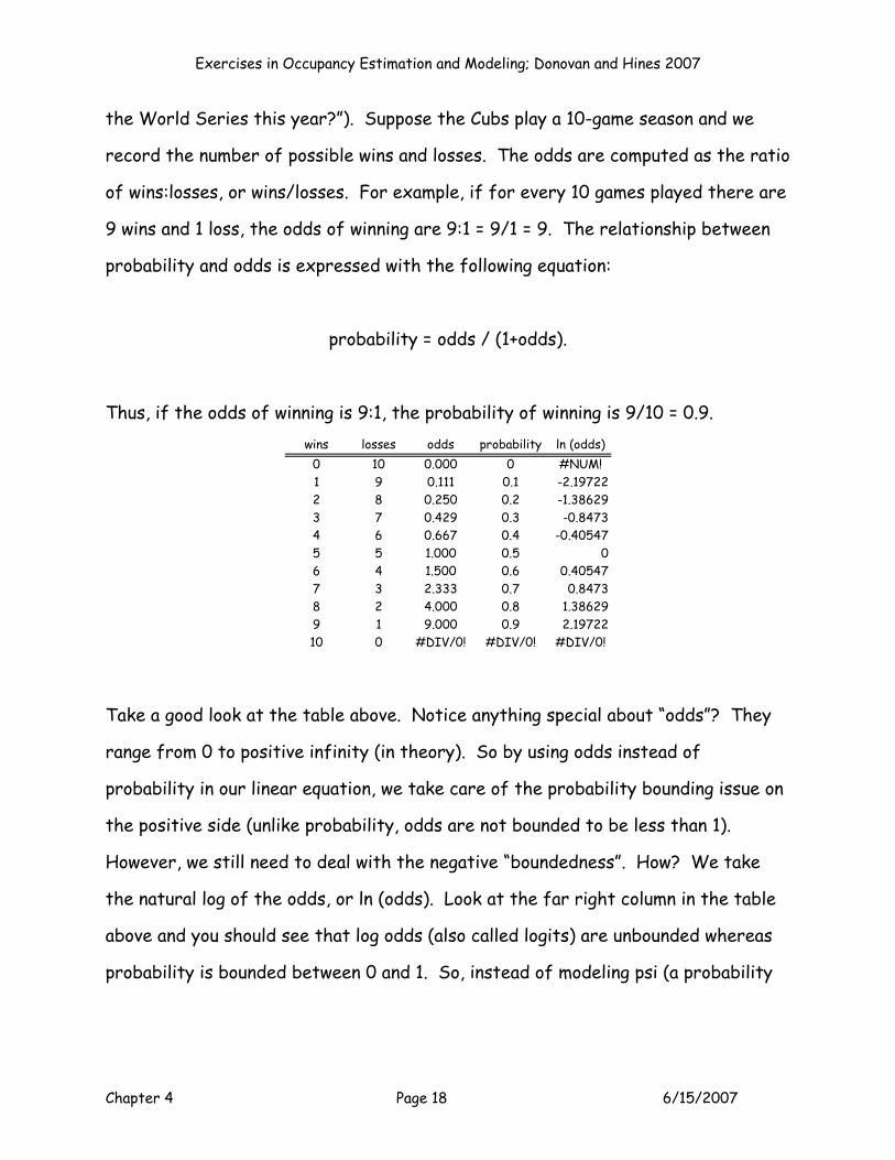
the World Series this year?”). Suppose the Cubs play a 10-game season and we
record the number of possible wins and losses. The odds are computed as the ratio
of wins:losses, or wins/losses. For example, if for every 10 games played there are
9 wins and 1 loss, the odds of winning are 9:1 = 9/1 = 9. The relationship between
probability and odds is expressed with the following equation:
probability = odds / (1+odds).
Thus, if the odds of winning is 9:1, the probability of winning is 9/10 = 0.9. wins losses odds probability ln (odds)
0 10 0.000 0 #NUM!1 9 0.111 0.1 -2.197222 8 0.250 0.2 -1.386293 7 0.429 0.3 -0.84734 6 0.667 0.4 -0.405475 5 1.000 0.5 06 4 1.500 0.6 0.405477 3 2.333 0.7 0.84738 2 4.000 0.8 1.386299 1 9.000 0.9 2.1972210 0 #DIV/0! #DIV/0! #DIV/0!
Take a good look at the table above. Notice anything special about “odds”? They
range from 0 to positive infinity (in theory). So by using odds instead of
probability in our linear equation, we take care of the probability bounding issue on
the positive side (unlike probability, odds are not bounded to be less than 1).
However, we still need to deal with the negative “boundedness”. How? We take
the natural log of the odds, or ln (odds). Look at the far right column in the table
above and you should see that log odds (also called logits) are unbounded whereas
probability is bounded between 0 and 1. So, instead of modeling psi (a probability
Exercises in Occupancy Estimation and Modeling; Donovan and Hines 2007
Chapter 4 Page 19 6/15/2007
bounded between 0 and 1), we model the log-odds of psi (which is unbounded). The
linear equation is now:
Logit psi = B0 + B1 * standardized patch size (which is a correctly specified linear model)
instead of
psi = B0 + B1 * standardized patch size (which is an incorrectly specified model)
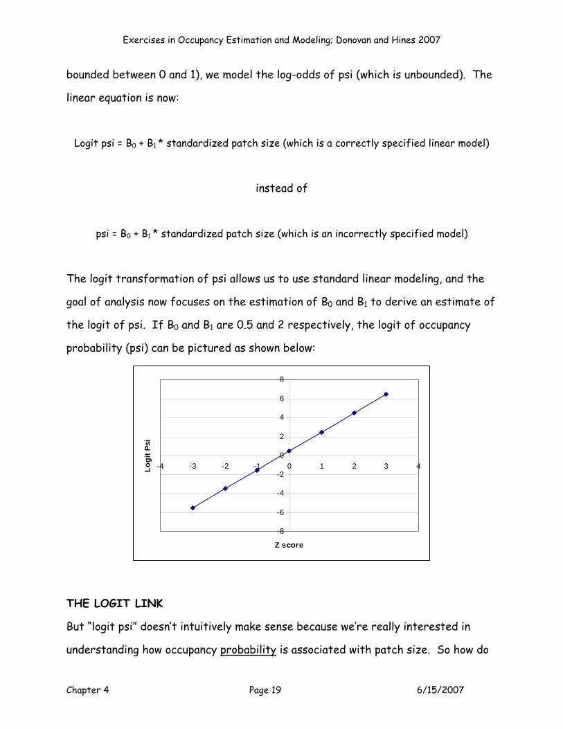
The logit transformation of psi allows us to use standard linear modeling, and the
goal of analysis now focuses on the estimation of B0 and B1 to derive an estimate of
the logit of psi. If B0 and B1 are 0.5 and 2 respectively, the logit of occupancy
probability (psi) can be pictured as shown below:
-8
-6
-4
-2
0
2
4
6
8
-4 -3 -2 -1 0 1 2 3 4
Z score
Logi
t Psi
THE LOGIT LINK
But “logit psi” doesn’t intuitively make sense because we’re really interested in
understanding how occupancy probability is associated with patch size. So how do
Exercises in Occupancy Estimation and Modeling; Donovan and Hines 2007
Chapter 4 Page 20 6/15/2007
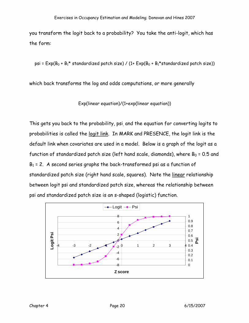
you transform the logit back to a probability? You take the anti-logit, which has
the form:
psi = Exp(B0 + B1* standardized patch size) / (1+ Exp(B0 + B1*standardized patch size))
which back transforms the log and odds computations, or more generally
Exp(linear equation)/(1+exp(linear equation))
This gets you back to the probability, psi, and the equation for converting logits to
probabilities is called the logit link. In MARK and PRESENCE, the logit link is the
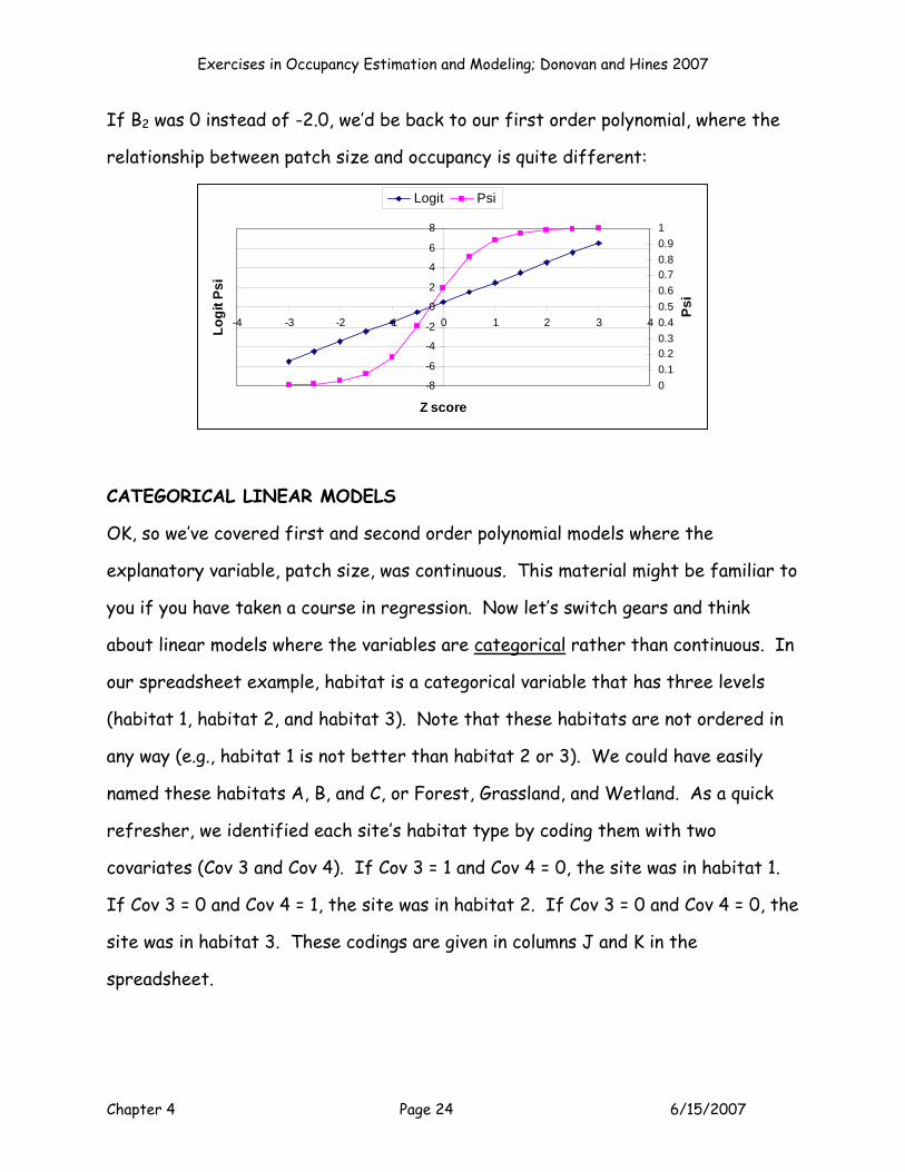
default link when covariates are used in a model. Below is a graph of the logit as a
function of standardized patch size (left hand scale, diamonds), where B0 = 0.5 and
B1 = 2. A second series graphs the back-transformed psi as a function of
standardized patch size (right hand scale, squares). Note the linear relationship
between logit psi and standardized patch size, whereas the relationship between
psi and standardized patch size is an s-shaped (logistic) function.
-8
-6
-4
-2
0
2
4
6
8
-4 -3 -2 -1 0 1 2 3 4
Z score
Logi
t Psi
00.10.20.30.40.50.60.70.80.91
Psi
Logit Psi
Exercises in Occupancy Estimation and Modeling; Donovan and Hines 2007
Chapter 4 Page 21 6/15/2007
How does this apply to our occupancy model? In this case, the anti-logit gives us
psi, and it does so for each site because we replace words “standardized patch
size” in the equation above with the Z patch size of each specific site. An example
might make this clearer. If B0 = 0.5 and B1 = 2, a site with a standardized patch
size of Z = +0.75 will have psi =Exp(0.5 + 2*0.75) / (1+ Exp(0.5 + 2*0.75))=0.8808,
whereas a site with a standardized patch size of Z = -0.75 would have
psi =Exp(0.5 + 2*-0.75) / (1+ Exp(0.5 + 2*-0.75))=0.26894. That’s quite a
difference in psi between the two sites! In this case, the site with a smaller patch
than average size (Z = -0.75) had a much lower occupancy probability (ψ = 0.26894)
than a site with a larger than average patch size (ψ = 0.8808). If you were to give
this model a name, you’d call it p(.)psi(patch size), indicating that psi is a function
of patch size (and p is the dot model where p1 = p2).
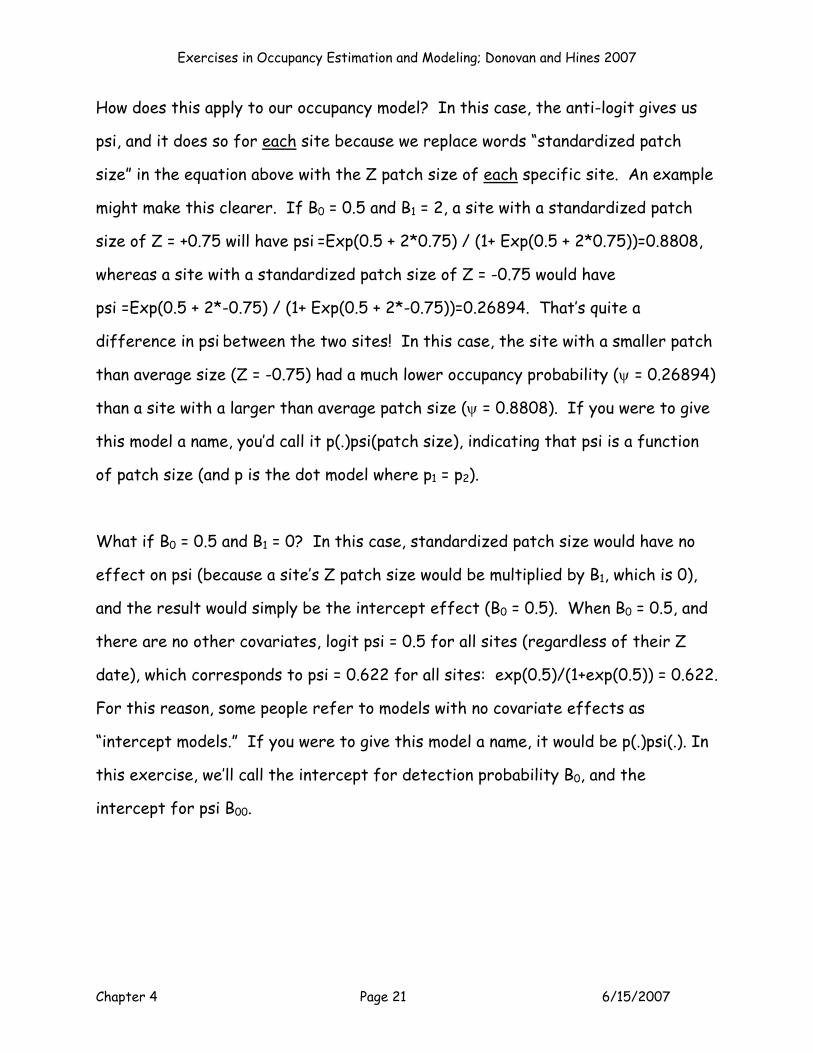
What if B0 = 0.5 and B1 = 0? In this case, standardized patch size would have no
effect on psi (because a site’s Z patch size would be multiplied by B1, which is 0),
and the result would simply be the intercept effect (B0 = 0.5). When B0 = 0.5, and
there are no other covariates, logit psi = 0.5 for all sites (regardless of their Z
date), which corresponds to psi = 0.622 for all sites: exp(0.5)/(1+exp(0.5)) = 0.622.
For this reason, some people refer to models with no covariate effects as
“intercept models.” If you were to give this model a name, it would be p(.)psi(.). In
this exercise, we’ll call the intercept for detection probability B0, and the
intercept for psi B00.
Exercises in Occupancy Estimation and Modeling; Donovan and Hines 2007
Chapter 4 Page 22 6/15/2007
0
0.1
0.2
0.3
0.4
0.5
0.6
-4 -3 -2 -1 0 1 2 3 4
Z score
Logi
t Psi
00.10.20.30.40.50.60.70.80.91
Psi
Logit Psi
Take some time with this material to make sure it really sinks in. There is also an
excellent discussion of this material in MARK: A Gentle Introduction by Evan Cooch
and Gary White. Darryl MacKenzie notes that you can also interpret things on the
odds scale, which is sometimes more intuitive than trying to interpret the effect
of a covariate on the standardized scale.
POLYNOMIAL LINEAR MODELS
OK! Now we are ready to move on to the second type of linear model that we will
explore: polynomial models. These are simple extensions of the models we just
discussed. A polynomial equation has the general form:
Y = B0 + B1X1 + B2X12 + B3X1
3 + …
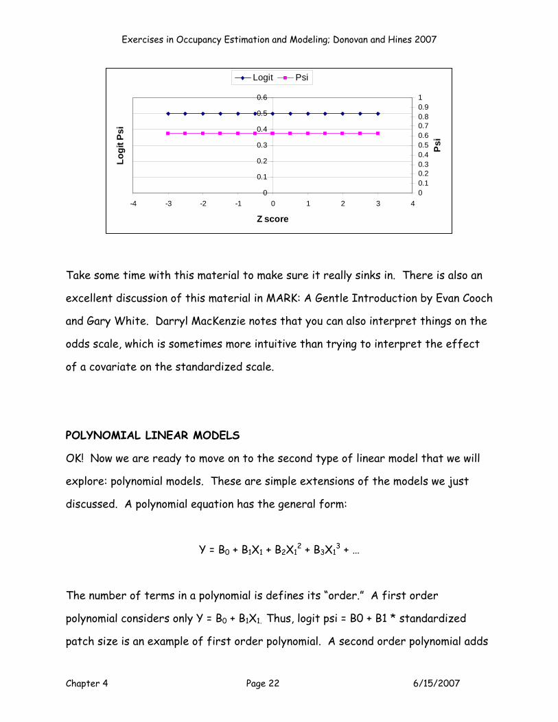
The number of terms in a polynomial is defines its “order.” A first order
polynomial considers only Y = B0 + B1X1. Thus, logit psi = B0 + B1 * standardized
patch size is an example of first order polynomial. A second order polynomial adds
Exercises in Occupancy Estimation and Modeling; Donovan and Hines 2007
Chapter 4 Page 23 6/15/2007
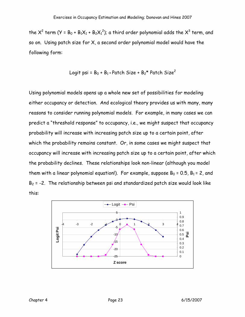
the X2 term (Y = B0 + B1X1 + B2X12); a third order polynomial adds the X3 term, and
so on. Using patch size for X, a second order polynomial model would have the
following form:
Logit psi = B0 + B1 * Patch Size + B2* Patch Size2
Using polynomial models opens up a whole new set of possibilities for modeling
either occupancy or detection. And ecological theory provides us with many, many
reasons to consider running polynomial models. For example, in many cases we can
predict a “threshold response” to occupancy, i.e., we might suspect that occupancy
probability will increase with increasing patch size up to a certain point, after
which the probability remains constant. Or, in some cases we might suspect that
occupancy will increase with increasing patch size up to a certain point, after which
the probability declines. These relationships look non-linear (although you model
them with a linear polynomial equation!). For example, suppose B0 = 0.5, B1 = 2, and
B2 = -2. The relationship between psi and standardized patch size would look like
this:
-25
-20
-15
-10
-5
0
5
-4 -3 -2 -1 0 1 2 3 4
Z score
Logi
t Psi
00.10.20.30.40.50.60.70.80.91
Psi
Logit Psi
Exercises in Occupancy Estimation and Modeling; Donovan and Hines 2007
Chapter 4 Page 24 6/15/2007
If B2 was 0 instead of -2.0, we’d be back to our first order polynomial, where the
relationship between patch size and occupancy is quite different:
-8
-6
-4
-2
0
2
4
6
8
-4 -3 -2 -1 0 1 2 3 4
Z score
Logi
t Psi
00.10.20.30.40.50.60.70.80.91
Psi
Logit Psi
CATEGORICAL LINEAR MODELS
OK, so we’ve covered first and second order polynomial models where the
explanatory variable, patch size, was continuous. This material might be familiar to
you if you have taken a course in regression. Now let’s switch gears and think
about linear models where the variables are categorical rather than continuous. In
our spreadsheet example, habitat is a categorical variable that has three levels
(habitat 1, habitat 2, and habitat 3). Note that these habitats are not ordered in
any way (e.g., habitat 1 is not better than habitat 2 or 3). We could have easily
named these habitats A, B, and C, or Forest, Grassland, and Wetland. As a quick
refresher, we identified each site’s habitat type by coding them with two
covariates (Cov 3 and Cov 4). If Cov 3 = 1 and Cov 4 = 0, the site was in habitat 1.
If Cov 3 = 0 and Cov 4 = 1, the site was in habitat 2. If Cov 3 = 0 and Cov 4 = 0, the
site was in habitat 3. These codings are given in columns J and K in the
spreadsheet.
Exercises in Occupancy Estimation and Modeling; Donovan and Hines 2007
Chapter 4 Page 25 6/15/2007
1314151617181920
G H I J K L MInt Cov 1 Cov 2 Cov 3 Cov 4 Cov 5 Cov 6
Psi (Int) Patch Size Patch Size 2 Habitat 1 Habitat 2 H1*PS H2*PS1 -1.9936 3.9743 1 0 -1.994 0.0001 0.9660 0.9332 0 0 0.000 0.0001 1.1794 1.3911 0 1 0.000 1.1791 -1.8955 3.5929 1 0 -1.895 0.0001 1.1377 1.2943 0 0 0.000 0.000
Occupancy Covariates
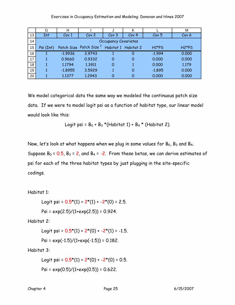
We model categorical data the same way we modeled the continuous patch size
data. If we were to model logit psi as a function of habitat type, our linear model
would look like this:
Logit psi = B0 + B3 *(Habitat 1) + B4 * (Habitat 2).
Now, let’s look at what happens when we plug in some values for B0, B3 and B4.
Suppose B0 = 0.5, B3 = 2, and B4 = -2. From these betas, we can derive estimates of
psi for each of the three habitat types by just plugging in the site-specific
codings.
Habitat 1:
Logit psi = 0.5*(1) + 2*(1) + -2*(0) = 2.5.
Psi = exp(2.5)/(1+exp(2.5)) = 0.924.
Habitat 2:
Logit psi = 0.5*(1) + 2*(0) + -2*(1) = -1.5.
Psi = exp(-1.5)/(1+exp(-1.5)) = 0.182.
Habitat 3:
Logit psi = 0.5*(1) + 2*(0) + -2*(0) = 0.5.
Psi = exp(0.5)/(1+exp(0.5)) = 0.622.

Exercises in Occupancy Estimation and Modeling; Donovan and Hines 2007
Chapter 4 Page 26 6/15/2007
Notice that the coding for habitat 3 (Cov 3 and Cov 4 = 0) renders just the
intercept. So, the probability of occupancy in habitat 3 is determined by the value
of the intercept of the linear model, which is true of any “reference” category.
We could graph these results as follows:
0
0.1
0.2
0.3
0.4
0.5
0.6
0.7
0.8
0.9
1
Habitat 1 Habitat 2 Habitat 3
Psi
Of course, you would need to include the standard errors of these estimates
before you can conclude whether habitat type truly influences occupancy
probability. This material is probably familiar to you if you’ve taken a statistics
course in Analysis of Variance.
ADDITIVE LINEAR MODELS
Now, what if psi was a function of both patch size and habitat? Well, we simply
expand our linear model to include the additional effects:
Logit psi = B0 + B1 * standardized patch size + B3 * habitat1 + B4 * habitat2.
And we can back-transform the logit to a probability with the logit link:
Exercises in Occupancy Estimation and Modeling; Donovan and Hines 2007
Chapter 4 Page 27 6/15/2007
psi = exp(B0 + B1 * standardized patch size + B3 * habitat1 + B4 * habitat2)/(1+exp(B0 + B1 *
standardized patch size + B3 * habitat1 + B4 * habitat2)).
This model would be called p(.)psi(patch size + habitat), and the focus of the
analysis would be on estimating B0, B1, B3 and B4 to derive psi for each site, as well
as the intercept for psi. This is called an additive model, because the effects are
simply added together and each piece of additional information (patch size,
habitat) simply builds on the other effects. A key assumption of additive models is
that the covariates are not influencing each other in any way, i.e., if you know the Z
score for patch size, it has no bearing on what the habitat is, other than a chance
relationship.
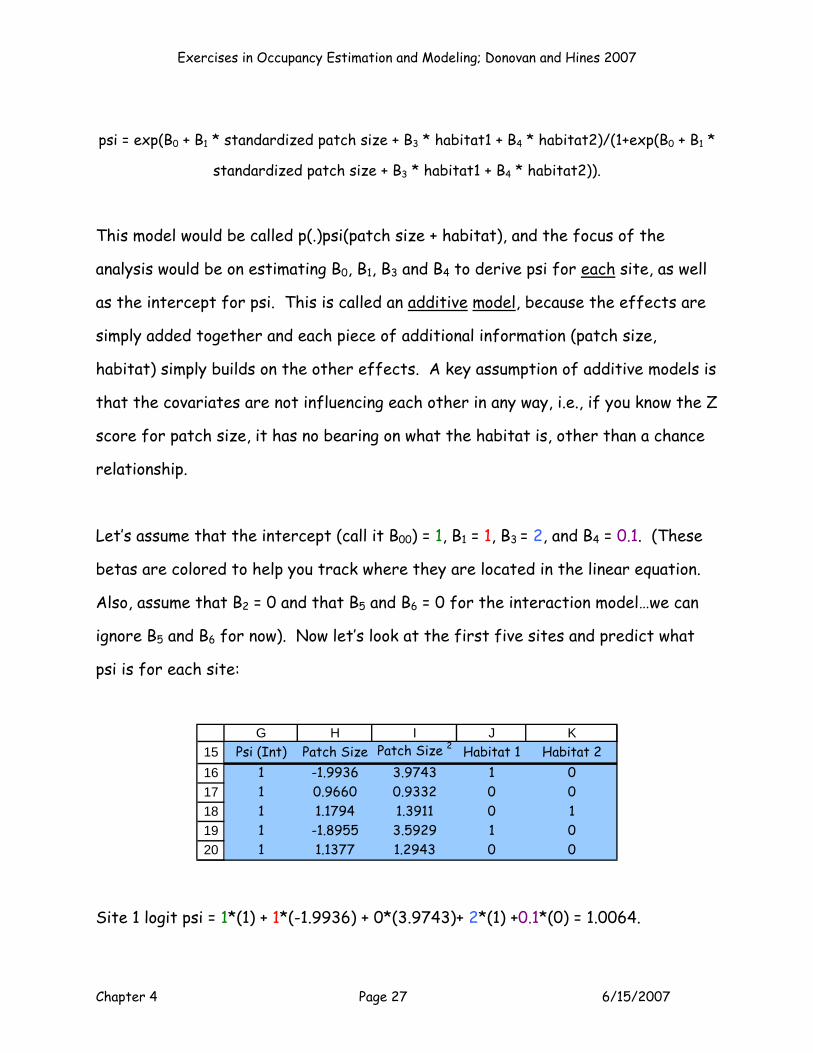
Let’s assume that the intercept (call it B00) = 1, B1 = 1, B3 = 2, and B4 = 0.1. (These
betas are colored to help you track where they are located in the linear equation.
Also, assume that B2 = 0 and that B5 and B6 = 0 for the interaction model…we can
ignore B5 and B6 for now). Now let’s look at the first five sites and predict what
psi is for each site:
151617181920
G H I J KPsi (Int) Patch Size Patch Size 2 Habitat 1 Habitat 2
1 -1.9936 3.9743 1 01 0.9660 0.9332 0 01 1.1794 1.3911 0 11 -1.8955 3.5929 1 01 1.1377 1.2943 0 0
Site 1 logit psi = 1*(1) + 1*(-1.9936) + 0*(3.9743)+ 2*(1) +0.1*(0) = 1.0064.
Exercises in Occupancy Estimation and Modeling; Donovan and Hines 2007
Chapter 4 Page 28 6/15/2007
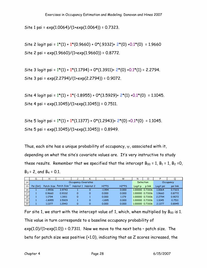
Site 1 psi = exp(1.0064)/(1+exp(1.0064)) = 0.7323.
Site 2 logit psi = 1*(1) + 1*(0.9660) + 0*(.9332)+ 2*(0) +0.1*(0) = 1.9660
Site 2 psi = exp(1.9660)/(1+exp(1.9660)) = 0.8772.
Site 3 logit psi = 1*(1) + 1*(1.1794) + 0*(1.3911)+ 2*(0) +0.1*(1) = 2.2794.
Site 3 psi = exp(2.2794)/(1+exp(2.2794)) = 0.9072.
Site 4 logit psi = 1*(1) + 1*(-1.8955) + 0*(3.5929)+ 2*(1) +0.1*(0) = 1.1045.
Site 4 psi = exp(1.1045)/(1+exp(1.1045)) = 0.7511.
Site 5 logit psi = 1*(1) + 1*(1.1377) + 0*(1.2943)+ 2*(0) +0.1*(0) = 1.1045.
Site 5 psi = exp(1.1045)/(1+exp(1.1045)) = 0.8949.
Thus, each site has a unique probability of occupancy, ψ, associated with it,
depending on what the site’s covariate values are. It’s very instructive to study
these results. Remember that we specified that the intercept B00 = 1, B1 = 1, B2 =0,
B3 = 2, and B4 = 0.1.
14151617181920
G H I J K L M N O P Q
Psi (Int) Patch Size Patch Size 2 Habitat 1 Habitat 2 H1*PS H2*PS Logit p p link Logit psi psi link1 -1.9936 3.9743 1 0 -1.994 0.000 1.00000 0.73106 1.0064 0.73231 0.9660 0.9332 0 0 0.000 0.000 1.00000 0.73106 1.9660 0.87721 1.1794 1.3911 0 1 0.000 1.179 1.00000 0.73106 2.2794 0.90721 -1.8955 3.5929 1 0 -1.895 0.000 1.00000 0.73106 1.1045 0.75111 1.1377 1.2943 0 0 0.000 0.000 1.00000 0.73106 2.1377 0.8945
Occupancy Covariates Detection Occupancy
For site 1, we start with the intercept value of 1, which, when multiplied by B00 is 1.
This value in turn corresponds to a baseline occupancy probability of
exp(1.0)/(1+exp(1.0)) = 0.7311. Now we move to the next beta – patch size. The
beta for patch size was positive (+1.0), indicating that as Z scores increased, the
Exercises in Occupancy Estimation and Modeling; Donovan and Hines 2007
Chapter 4 Page 29 6/15/2007
probability of occupancy increased. Site 1 was much smaller than the average
patch (Z score of -1.9936) which decreased the probability of occupancy below the
baseline value: exp(1 + -1.9936)/(1+exp(1 + -1.9936)) = 0.2702. Now we move to the
habitat betas. If site 1 was located in habitat 3, the final probability of occupancy
would remain at 0.2702. However, the fact site 1 was located in habitat 1
effectively reversed the negative effect of patch size (the beta for habitat 1 was
+2.0, which is a very strong effect: exp(1 + -1.9936 + 2.0)/(1+exp(1 + -1.9936 +
2.0)) = 0.7323. Essentially, by being in habitat 1, the intercept is bumped up by 2
logit notches, with the final probability of occupancy for site 1 = 0.7323. Site 2
had a higher probability of occupancy than site 1: it was located in habitat 3 (the
reference habitat), but because it had a larger than average patch size (Z =
0.9960), the probability of occupancy increased. Site 3 had a very high probability
of occupancy (0.9072) because it had a large patch size (Z = 1.1794), and the
probability was also slightly increased because site 3 was located in habitat 2. It’s
worthwhile to take the time to understand exactly what the betas mean, and
assess the magnitude of their effects.
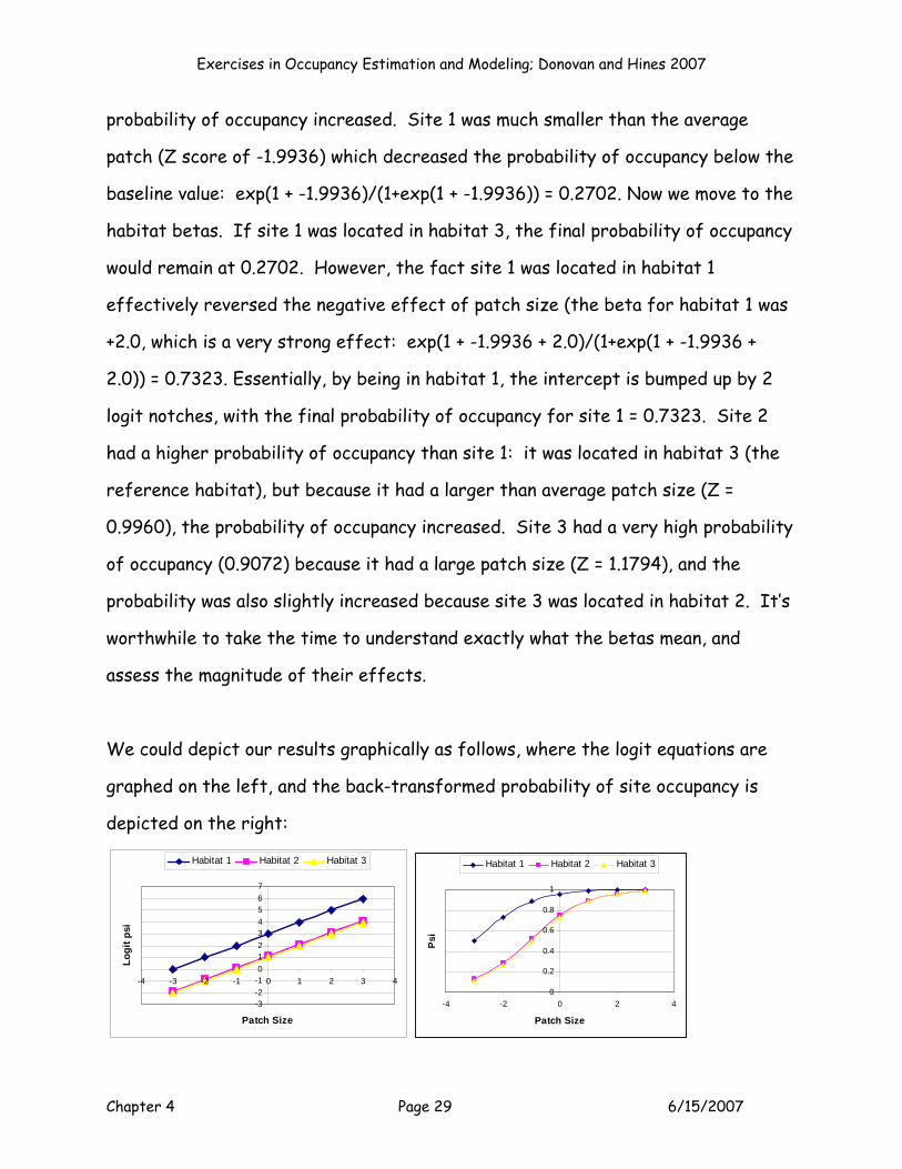
We could depict our results graphically as follows, where the logit equations are
graphed on the left, and the back-transformed probability of site occupancy is
depicted on the right:
-3-2-101234567
-4 -3 -2 -1 0 1 2 3 4
Patch Size
Logi
t psi
Habitat 1 Habitat 2 Habitat 3
0
0.2
0.4
0.6
0.8
1
-4 -2 0 2 4
Patch Size
Psi
Habitat 1 Habitat 2 Habitat 3
Exercises in Occupancy Estimation and Modeling; Donovan and Hines 2007
Chapter 4 Page 30 6/15/2007
It’s critical that you understand a fundamental point for additive models: the
effect of the continuous variable (i.e., the slope of the effect) is the same for all
categories (habitats); the effect of the categories (habitat) themselves simply
shift the intercept up or down relative to the reference category (in this case,
habitat 3). Thus, graphs of the logit equations show that the effect of patch size
on occupancy is the same for all habitat types (occupancy probability increases as
patch size increases), but the habitats themselves may have different baseline
occupancy levels. If you’ve had a statistics course in linear modeling, you might
recognize this model as an Analysis of Covariance (equal slopes model).
LINEAR MODELS WITH INTERACTIVE EFFECTS
The last type of linear model that we will examine is the model that includes
interactions between patch size and habitat. This model is a bit of a mind-bender,
but it’s not too bad if you spend a bit of time on it. In our example, an interaction
between patch size and habitat can be interpreted as follows: the effect of patch
size on occupancy depends on what habitat you are considering. So, you need to
talk about the effect of patch size for each habitat separately. The interaction
between patch size and habitat requires two additional parameters be estimated:
B5 and B6. Additionally, you need to “create” the 2 new pieces of interaction data
for each site. First, multiply patch size by habitat 1. Second, multiply patch size
by habitat 2. The results are shown in columns L and M. Thus, column L contains a
non-zero patch size value for sites located in habitat 1, while column M contains a
non-zero patch size value for sites located in habitat 2. (I don’t know if
standardization affects the interaction model outcomes or not.) The full linear
model becomes:
Exercises in Occupancy Estimation and Modeling; Donovan and Hines 2007
Chapter 4 Page 31 6/15/2007
Logit psi = B0 + B1 * (patch size) + B2 * (patch size2) + B3 * (habitat1) + B4 * (habitat2) + B5
* (patch size*habitat1) + B6 * (patch size*habitat2).
If B5 is significantly different from 0, there is evidence that the effect of patch
size for habitat 1 differs from the other two habitats; if B6 is significantly
different from 0, there is evidence that the effect (slope) of patch size for
habitat 2 differs from the other two habitats. If B5 and B6 are both 0, then there
is no evidence of a patch size by habitat interaction, and you’re back to the
additive model (patch size + habitat), in which the effect of patch size is the same
for all habitat types.
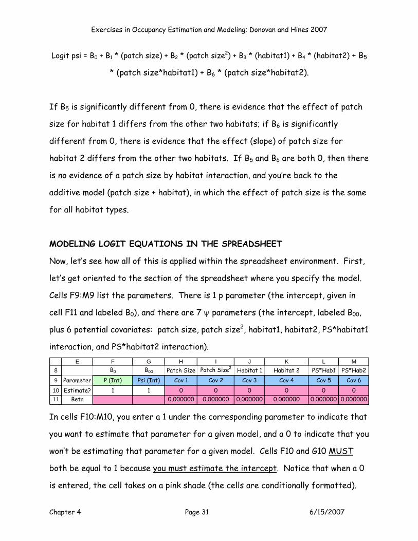
MODELING LOGIT EQUATIONS IN THE SPREADSHEET
Now, let’s see how all of this is applied within the spreadsheet environment. First,
let’s get oriented to the section of the spreadsheet where you specify the model.
Cells F9:M9 list the parameters. There is 1 p parameter (the intercept, given in
cell F11 and labeled B0), and there are 7 ψ parameters (the intercept, labeled B00,
plus 6 potential covariates: patch size, patch size2, habitat1, habitat2, PS*habitat1
interaction, and PS*habitat2 interaction).
8
9
1011
E F G H I J K L MB0 B00 Patch Size Patch Size2 Habitat 1 Habitat 2 PS*Hab1 PS*Hab2
Parameter P (Int) Psi (Int) Cov 1 Cov 2 Cov 3 Cov 4 Cov 5 Cov 6Estimate? 1 1 0 0 0 0 0 0
Beta 0.000000 0.000000 0.000000 0.000000 0.000000 0.000000
In cells F10:M10, you enter a 1 under the corresponding parameter to indicate that
you want to estimate that parameter for a given model, and a 0 to indicate that you
won’t be estimating that parameter for a given model. Cells F10 and G10 MUST
both be equal to 1 because you must estimate the intercept. Notice that when a 0
is entered, the cell takes on a pink shade (the cells are conditionally formatted).

Exercises in Occupancy Estimation and Modeling; Donovan and Hines 2007
Chapter 4 Page 32 6/15/2007
Underneath the “Estimate?” row is the Beta row. Solver will work on finding the
values in these cells, so you should make sure they are blank before running Solver,
with the exception that you must enter a 0 in those cells for any parameter that is
not being estimated. (Thus, if a certain parameter is not being estimated, the
“Estimate?” cell will be pink, and you must enter a 0 in its corresponding beta
beneath it). This is necessary to count the number of parameters estimated
correctly, and to ensure that logits for p and ψ are computed correctly. So, the
model shown above is set up to estimate the intercept for p and the intercept for
psi. In other words, the model depicted is p(.)psi(.). By forcing the betas for all
covariate effects to be 0, the covariates do not enter the linear equation for
estimating the logit of p or the logit of psi. In this example, Solver will find values
for cells F11 and G11 that maximize the multinomial log likelihood.
Now let’s look at how the spreadsheet computes logit p, p, logit ψ, and ψ for each
site. First, clear out the beta cells (F11:M11).
141516
N O P Q
Logit p p link Logit ψ ψ link0.00000 0.50000 0.0000 0.5000
Detection Occupancy
Cell N16 (logit p for site 1) has the equation =F16*$F$11, which computes the logit
for p. It’s basically taking the beta values for p, and multiplying them by the
intercept value for site 1 (which is 1 for all sites). The logit link is computed in cell
O16 with the equation =EXP(N16)/(1+EXP(N16)). In other words,
P = Exp(B0)/(1+exp(B0)). These two equations are copied down columns to generate
the logit p and p for the remaining sites. Note that since this is a p(.) model, p1 =
p2, and p is the same for all 200 sites.
Exercises in Occupancy Estimation and Modeling; Donovan and Hines 2007
Chapter 4 Page 33 6/15/2007
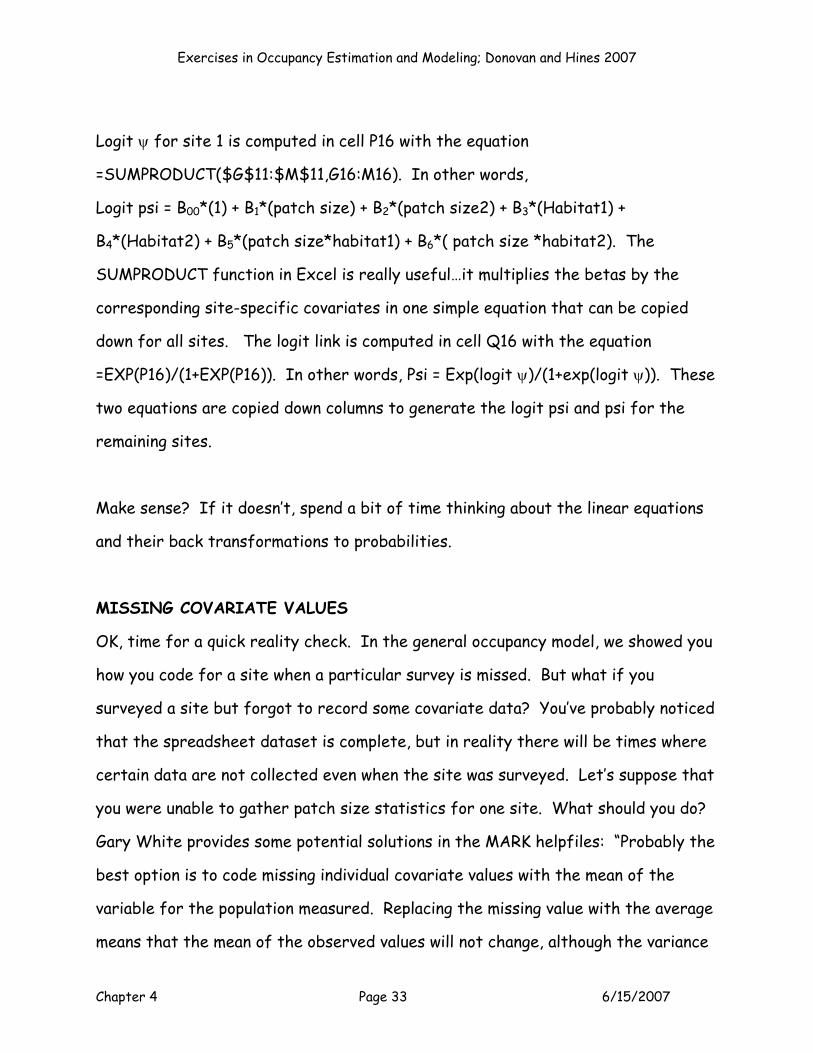
Logit ψ for site 1 is computed in cell P16 with the equation
=SUMPRODUCT($G$11:$M$11,G16:M16). In other words,
Logit psi = B00*(1) + B1*(patch size) + B2*(patch size2) + B3*(Habitat1) +
B4*(Habitat2) + B5*(patch size*habitat1) + B6*( patch size *habitat2). The
SUMPRODUCT function in Excel is really useful…it multiplies the betas by the
corresponding site-specific covariates in one simple equation that can be copied
down for all sites. The logit link is computed in cell Q16 with the equation
=EXP(P16)/(1+EXP(P16)). In other words, Psi = Exp(logit ψ)/(1+exp(logit ψ)). These
two equations are copied down columns to generate the logit psi and psi for the
remaining sites.
Make sense? If it doesn’t, spend a bit of time thinking about the linear equations
and their back transformations to probabilities.
MISSING COVARIATE VALUES
OK, time for a quick reality check. In the general occupancy model, we showed you
how you code for a site when a particular survey is missed. But what if you
surveyed a site but forgot to record some covariate data? You’ve probably noticed
that the spreadsheet dataset is complete, but in reality there will be times where
certain data are not collected even when the site was surveyed. Let’s suppose that
you were unable to gather patch size statistics for one site. What should you do?
Gary White provides some potential solutions in the MARK helpfiles: “Probably the
best option is to code missing individual covariate values with the mean of the
variable for the population measured. Replacing the missing value with the average
means that the mean of the observed values will not change, although the variance
Exercises in Occupancy Estimation and Modeling; Donovan and Hines 2007
Chapter 4 Page 34 6/15/2007
will be slightly smaller because all missing values will be exactly equal to the mean
and hence not variable. If you have lots of missing values, another option is to
code the sites into 2 groups, where all the missing values are in one group. Then,
you can use both groups to estimate a common parameter, and only apply the
individual covariate to one group. This approach can be tricky, so think through
what you are doing before you try this approach.” Alternatively, if relatively few
sites have missing data, it might be best just to omit them from analysis.
MODEL P(.)PSI(.)
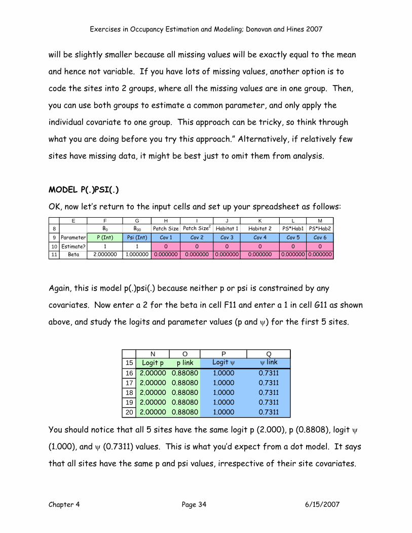
OK, now let’s return to the input cells and set up your spreadsheet as follows:
8
9
1011
E F G H I J K L MB0 B00 Patch Size Patch Size2 Habitat 1 Habitat 2 PS*Hab1 PS*Hab2
Parameter P (Int) Psi (Int) Cov 1 Cov 2 Cov 3 Cov 4 Cov 5 Cov 6Estimate? 1 1 0 0 0 0 0 0
Beta 2.000000 1.000000 0.000000 0.000000 0.000000 0.000000 0.000000 0.000000
Again, this is model p(.)psi(.) because neither p or psi is constrained by any
covariates. Now enter a 2 for the beta in cell F11 and enter a 1 in cell G11 as shown
above, and study the logits and parameter values (p and ψ) for the first 5 sites.
151617181920
N O P QLogit p p link Logit ψ ψ link
2.00000 0.88080 1.0000 0.73112.00000 0.88080 1.0000 0.73112.00000 0.88080 1.0000 0.73112.00000 0.88080 1.0000 0.73112.00000 0.88080 1.0000 0.7311
You should notice that all 5 sites have the same logit p (2.000), p (0.8808), logit ψ
(1.000), and ψ (0.7311) values. This is what you’d expect from a dot model. It says
that all sites have the same p and psi values, irrespective of their site covariates.

Exercises in Occupancy Estimation and Modeling; Donovan and Hines 2007
Chapter 4 Page 35 6/15/2007
If you change the values in cells F11 or J11, you’ll see different p and psi estimates,
but the new estimates will be the same for all sites. Try it!
Now, in the basic occupancy model we mentioned model over-parameterization.
Recall that the saturated model for the basic model (with no covariates) estimates
a probability of each history based on the raw data. In this particular example,
there are 4 kinds of histories (11, 10, 01, and 00), and the sum of the history
probabilities must be 1. Therefore, for this particular data set where no
covariates are estimated, you can estimate 4 – 1 = 3 parameters at most, otherwise
the model will be overparamaterized (there are 3 “free” parameters in the
multinomial equation – the fourth is not free because you can derive it). What
about the covariate model? Well, with the covariate model, each site has a unique
probability of detection and occupancy (depending on the model), so the saturated
model does not really apply because the analysis is done on a site by site basis.
Does this mean you can run a model with 100 covariates? No! The general rule of
thumb is that you need at least 10 observations (sites) per parameter estimated
(more is much better, otherwise you are asking too much from a small number of
sample points). In this spreadsheet example, we have 200 sites, so we could run a
model with up to 20 parameters, though that wouldn’t be advisable. Suppose that
you conducted a study where only 50 sites were evaluated. This means that you
can run models with ≤ 5 parameters. It sounds like a lot of sites, but remember
that you must estimate the intercept for p and the intercept for ψ, so you have
only three covariates to “play” with in any one model.
MODEL P(.)PSI(Patch Size)
Exercises in Occupancy Estimation and Modeling; Donovan and Hines 2007
Chapter 4 Page 36 6/15/2007
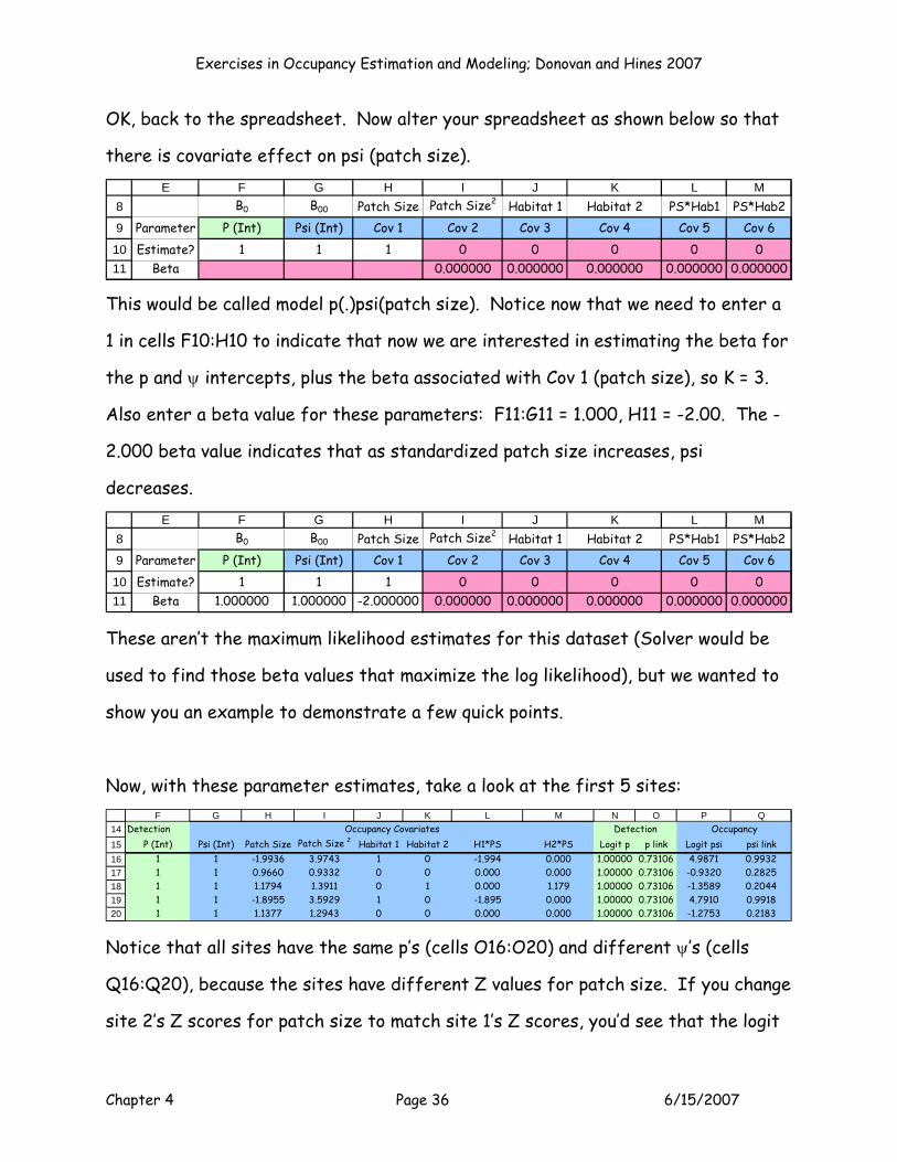
OK, back to the spreadsheet. Now alter your spreadsheet as shown below so that
there is covariate effect on psi (patch size).
8
9
1011
E F G H I J K L MB0 B00 Patch Size Patch Size2 Habitat 1 Habitat 2 PS*Hab1 PS*Hab2
Parameter P (Int) Psi (Int) Cov 1 Cov 2 Cov 3 Cov 4 Cov 5 Cov 6Estimate? 1 1 1 0 0 0 0 0
Beta 0.000000 0.000000 0.000000 0.000000 0.000000
This would be called model p(.)psi(patch size). Notice now that we need to enter a
1 in cells F10:H10 to indicate that now we are interested in estimating the beta for
the p and ψ intercepts, plus the beta associated with Cov 1 (patch size), so K = 3.
Also enter a beta value for these parameters: F11:G11 = 1.000, H11 = -2.00. The -
2.000 beta value indicates that as standardized patch size increases, psi
decreases.
8
9
1011
E F G H I J K L MB0 B00 Patch Size Patch Size2 Habitat 1 Habitat 2 PS*Hab1 PS*Hab2
Parameter P (Int) Psi (Int) Cov 1 Cov 2 Cov 3 Cov 4 Cov 5 Cov 6Estimate? 1 1 1 0 0 0 0 0
Beta 1.000000 1.000000 -2.000000 0.000000 0.000000 0.000000 0.000000 0.000000
These aren’t the maximum likelihood estimates for this dataset (Solver would be
used to find those beta values that maximize the log likelihood), but we wanted to
show you an example to demonstrate a few quick points.
Now, with these parameter estimates, take a look at the first 5 sites:
14151617181920
F G H I J K L M N O P QDetection
P (Int) Psi (Int) Patch Size Patch Size 2 Habitat 1 Habitat 2 H1*PS H2*PS Logit p p link Logit psi psi link1 1 -1.9936 3.9743 1 0 -1.994 0.000 1.00000 0.73106 4.9871 0.99321 1 0.9660 0.9332 0 0 0.000 0.000 1.00000 0.73106 -0.9320 0.28251 1 1.1794 1.3911 0 1 0.000 1.179 1.00000 0.73106 -1.3589 0.20441 1 -1.8955 3.5929 1 0 -1.895 0.000 1.00000 0.73106 4.7910 0.99181 1 1.1377 1.2943 0 0 0.000 0.000 1.00000 0.73106 -1.2753 0.2183
Occupancy Covariates Detection Occupancy
Notice that all sites have the same p’s (cells O16:O20) and different ψ’s (cells
Q16:Q20), because the sites have different Z values for patch size. If you change
site 2’s Z scores for patch size to match site 1’s Z scores, you’d see that the logit
Exercises in Occupancy Estimation and Modeling; Donovan and Hines 2007
Chapter 4 Page 37 6/15/2007
psi and ψ would be identical for both sites because the two sites have exactly the
same covariate values.
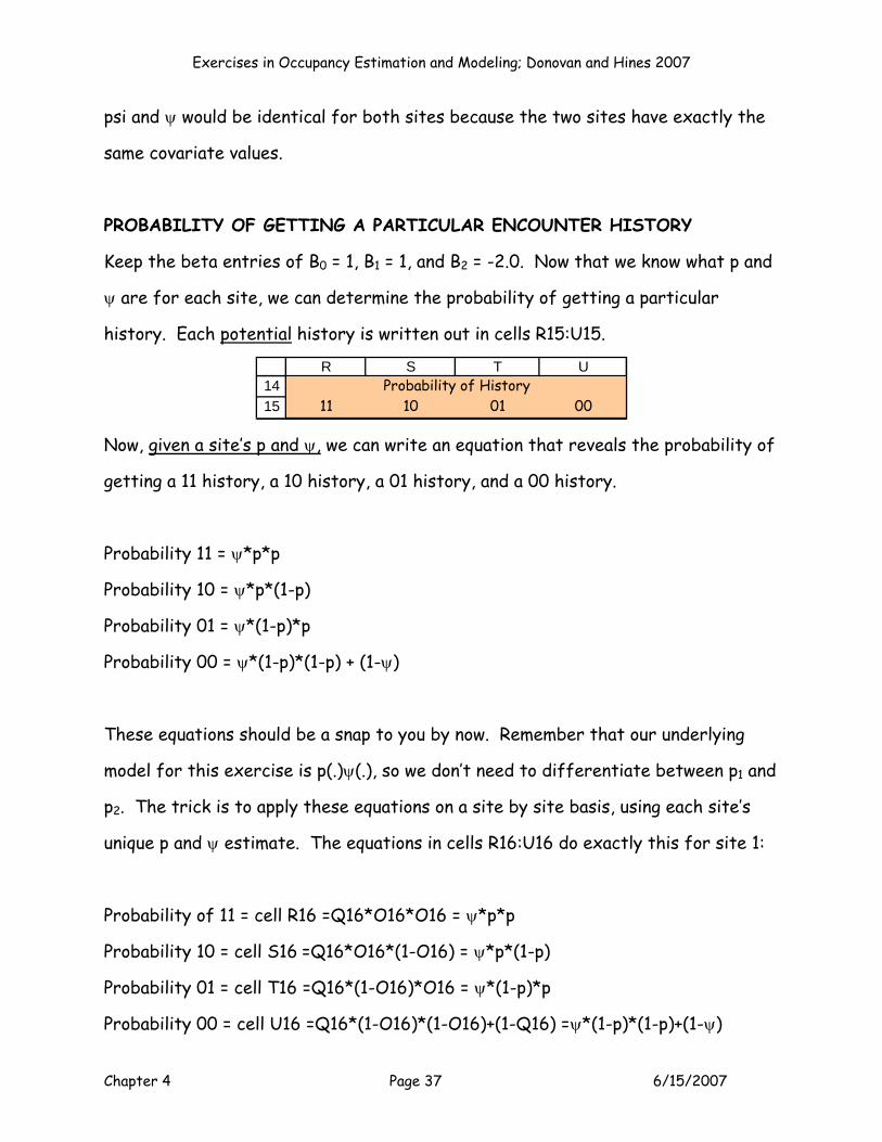
PROBABILITY OF GETTING A PARTICULAR ENCOUNTER HISTORY
Keep the beta entries of B0 = 1, B1 = 1, and B2 = -2.0. Now that we know what p and
ψ are for each site, we can determine the probability of getting a particular
history. Each potential history is written out in cells R15:U15.
1415
R S T U
11 10 01 00Probability of History
Now, given a site’s p and ψ, we can write an equation that reveals the probability of
getting a 11 history, a 10 history, a 01 history, and a 00 history.
Probability 11 = ψ*p*p
Probability 10 = ψ*p*(1-p)
Probability 01 = ψ*(1-p)*p
Probability 00 = ψ*(1-p)*(1-p) + (1-ψ)
These equations should be a snap to you by now. Remember that our underlying
model for this exercise is p(.)ψ(.), so we don’t need to differentiate between p1 and
p2. The trick is to apply these equations on a site by site basis, using each site’s
unique p and ψ estimate. The equations in cells R16:U16 do exactly this for site 1:
Probability of 11 = cell R16 =Q16*O16*O16 = ψ*p*p
Probability 10 = cell S16 =Q16*O16*(1-O16) = ψ*p*(1-p)
Probability 01 = cell T16 =Q16*(1-O16)*O16 = ψ*(1-p)*p
Probability 00 = cell U16 =Q16*(1-O16)*(1-O16)+(1-Q16) =ψ*(1-p)*(1-p)+(1-ψ)
Exercises in Occupancy Estimation and Modeling; Donovan and Hines 2007
Chapter 4 Page 38 6/15/2007
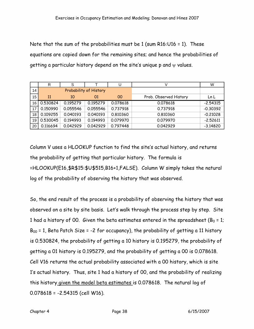
Note that the sum of the probabilities must be 1 (sum R16:U16 = 1). These
equations are copied down for the remaining sites; and hence the probabilities of
getting a particular history depend on the site’s unique p and ψ values.
14151617181920
R S T U V W
11 10 01 00 Prob. Observed History Ln L 0.530824 0.195279 0.195279 0.078618 0.078618 -2.543150.150990 0.055546 0.055546 0.737918 0.737918 -0.303920.109255 0.040193 0.040193 0.810360 0.810360 -0.210280.530045 0.194993 0.194993 0.079970 0.079970 -2.526110.116694 0.042929 0.042929 0.797448 0.042929 -3.14820
Probability of History
Column V uses a HLOOKUP function to find the site’s actual history, and returns
the probability of getting that particular history. The formula is
=HLOOKUP(E16,$R$15:$U$515,B16+1,FALSE). Column W simply takes the natural
log of the probability of observing the history that was observed.
So, the end result of the process is a probability of observing the history that was
observed on a site by site basis. Let’s walk through the process step by step. Site
1 had a history of 00. Given the beta estimates entered in the spreadsheet (B0 = 1;
B00 = 1, Beta Patch Size = -2 for occupancy), the probability of getting a 11 history
is 0.530824, the probability of getting a 10 history is 0.195279, the probability of
getting a 01 history is 0.195279, and the probability of getting a 00 is 0.078618.
Cell V16 returns the actual probability associated with a 00 history, which is site
1’s actual history. Thus, site 1 had a history of 00, and the probability of realizing
this history given the model beta estimates is 0.078618. The natural log of
0.078618 = -2.54315 (cell W16).
Exercises in Occupancy Estimation and Modeling; Donovan and Hines 2007
Chapter 4 Page 39 6/15/2007
141516
R S T U V W
11 10 01 00 Prob. Observed History Ln L 0.530824 0.195279 0.195279 0.078618 0.078618 -2.54315
Probability of History
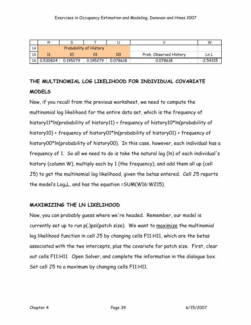
THE MULTINOMIAL LOG LIKELIHOOD FOR INDIVIDUAL COVARIATE
MODELS
Now, if you recall from the previous worksheet, we need to compute the
multinomial log likelihood for the entire data set, which is the frequency of
history11*ln(probability of history11) + frequency of history10*ln(probability of
history10) + frequency of history01*ln(probability of history01) + frequency of
history00*ln(probability of history00). In this case, however, each individual has a
frequency of 1. So all we need to do is take the natural log (ln) of each individual's
history (column W), multiply each by 1 (the frequency), and add them all up (cell
J5) to get the multinomial log likelihood, given the betas entered. Cell J5 reports
the model’s LogeL, and has the equation =SUM(W16:W215).
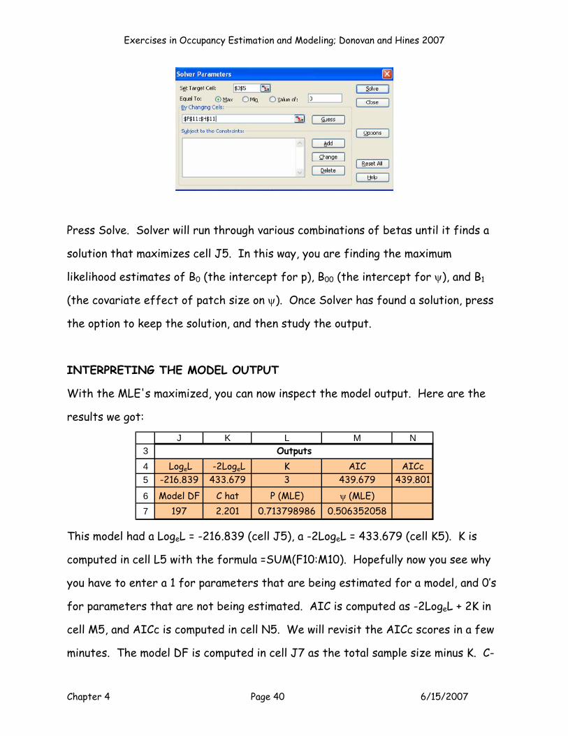
MAXIMIZING THE LN LIKELIHOOD
Now, you can probably guess where we're headed. Remember, our model is
currently set up to run p(.)psi(patch size). We want to maximize the multinomial
log likelihood function in cell J5 by changing cells F11:H11, which are the betas
associated with the two intercepts, plus the covariate for patch size. First, clear
out cells F11:H11. Open Solver, and complete the information in the dialogue box.
Set cell J5 to a maximum by changing cells F11:H11.
Exercises in Occupancy Estimation and Modeling; Donovan and Hines 2007
Chapter 4 Page 40 6/15/2007
Press Solve. Solver will run through various combinations of betas until it finds a
solution that maximizes cell J5. In this way, you are finding the maximum
likelihood estimates of B0 (the intercept for p), B00 (the intercept for ψ), and B1
(the covariate effect of patch size on ψ). Once Solver has found a solution, press
the option to keep the solution, and then study the output.
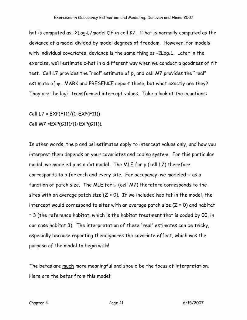
INTERPRETING THE MODEL OUTPUT
With the MLE's maximized, you can now inspect the model output. Here are the
results we got:
3
45
67
J K L M N
LogeL -2LogeL K AIC AICc-216.839 433.679 3 439.679 439.801Model DF C hat P (MLE) ψ (MLE)
197 2.201 0.713798986 0.506352058
Outputs
This model had a LogeL = -216.839 (cell J5), a -2LogeL = 433.679 (cell K5). K is
computed in cell L5 with the formula =SUM(F10:M10). Hopefully now you see why
you have to enter a 1 for parameters that are being estimated for a model, and 0’s
for parameters that are not being estimated. AIC is computed as -2LogeL + 2K in
cell M5, and AICc is computed in cell N5. We will revisit the AICc scores in a few
minutes. The model DF is computed in cell J7 as the total sample size minus K. C-
Exercises in Occupancy Estimation and Modeling; Donovan and Hines 2007
Chapter 4 Page 41 6/15/2007
hat is computed as -2LogeL/model DF in cell K7. C-hat is normally computed as the
deviance of a model divided by model degrees of freedom. However, for models
with individual covariates, deviance is the same thing as -2LogeL. Later in the
exercise, we’ll estimate c-hat in a different way when we conduct a goodness of fit
test. Cell L7 provides the “real” estimate of p, and cell M7 provides the “real”
estimate of ψ. MARK and PRESENCE report these, but what exactly are they?
They are the logit transformed intercept values. Take a look at the equations:
Cell L7 = EXP(F11)/(1+EXP(F11))
Cell M7 =EXP(G11)/(1+EXP(G11)).
In other words, the p and psi estimates apply to intercept values only, and how you
interpret them depends on your covariates and coding system. For this particular
model, we modeled p as a dot model. The MLE for p (cell L7) therefore
corresponds to p for each and every site. For occupancy, we modeled ψ as a
function of patch size. The MLE for ψ (cell M7) therefore corresponds to the
sites with an average patch size (Z = 0). If we included habitat in the model, the
intercept would correspond to sites with an average patch size (Z = 0) and habitat
= 3 (the reference habitat, which is the habitat treatment that is coded by 00, in
our case habitat 3). The interpretation of these “real” estimates can be tricky,
especially because reporting them ignores the covariate effect, which was the
purpose of the model to begin with!
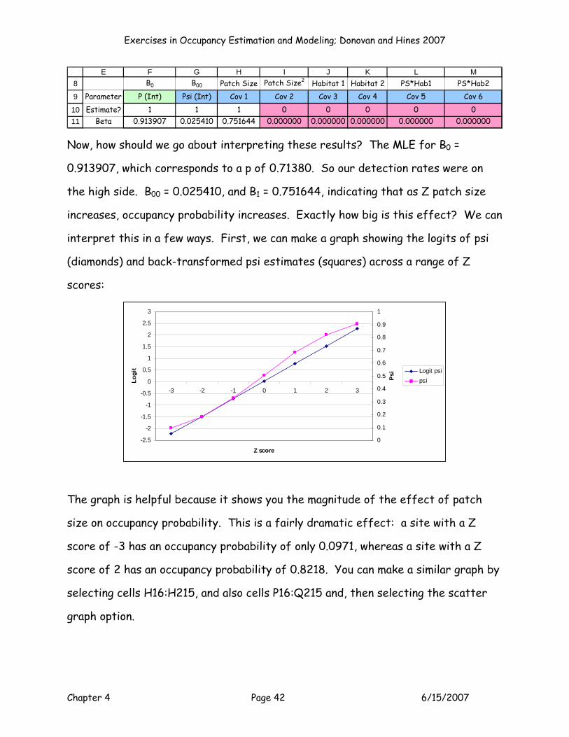
The betas are much more meaningful and should be the focus of interpretation.
Here are the betas from this model:
Exercises in Occupancy Estimation and Modeling; Donovan and Hines 2007
Chapter 4 Page 42 6/15/2007
8
9
1011
E F G H I J K L MB0 B00 Patch Size Patch Size2 Habitat 1 Habitat 2 PS*Hab1 PS*Hab2
Parameter P (Int) Psi (Int) Cov 1 Cov 2 Cov 3 Cov 4 Cov 5 Cov 6Estimate? 1 1 1 0 0 0 0 0
Beta 0.913907 0.025410 0.751644 0.000000 0.000000 0.000000 0.000000 0.000000
Now, how should we go about interpreting these results? The MLE for B0 =
0.913907, which corresponds to a p of 0.71380. So our detection rates were on
the high side. B00 = 0.025410, and B1 = 0.751644, indicating that as Z patch size
increases, occupancy probability increases. Exactly how big is this effect? We can
interpret this in a few ways. First, we can make a graph showing the logits of psi
(diamonds) and back-transformed psi estimates (squares) across a range of Z
scores:
-2.5
-2
-1.5
-1
-0.5
0
0.5
1
1.5
2
2.5
3
-3 -2 -1 0 1 2 3
Z score
Logi
t
0
0.1
0.2
0.3
0.4
0.5
0.6
0.7
0.8
0.9
1
Psi Logit psi
psi
The graph is helpful because it shows you the magnitude of the effect of patch
size on occupancy probability. This is a fairly dramatic effect: a site with a Z
score of -3 has an occupancy probability of only 0.0971, whereas a site with a Z
score of 2 has an occupancy probability of 0.8218. You can make a similar graph by
selecting cells H16:H215, and also cells P16:Q215 and, then selecting the scatter
graph option.
Exercises in Occupancy Estimation and Modeling; Donovan and Hines 2007
Chapter 4 Page 43 6/15/2007
If B1 = 0.1 instead of 0.751644, the effect would be much less dramatic.
-2.5
-1.5
-0.5
0.5
1.5
2.5
-3 -2 -1 0 1 2 3
Z score
Logi
t
0
0.1
0.2
0.3
0.4
0.5
0.6
0.7
0.8
0.9
1
Psi Logit psi
psi
With B1 = 0.1, a site with a Z score -3 for patch size has a 0.4318 probability of
detection, while a site with a Z score of +2 for patch size has a 0.5561 probability
of detection…not nearly as dramatic.
Second, we can discuss this result in terms of odds, which is computed as
probability/(1-probability). Given that B00 = 0.025410 and B1 = 0.7516440, the

Exercises in Occupancy Estimation and Modeling; Donovan and Hines 2007
Chapter 4 Page 44 6/15/2007
probability of occupancy at a site where Z = +2.0 is exp(0.025410 +
0.7516440*2)/(1+exp(0.025410 +0.7516440*2)) = 0.8218. The odds of a species
being detected on at this site are then computed as:
0.8218/(1-0.8218) = 4.611672.
Therefore, the odds are 4.61:1. Remember, odds is interpreted as wins:losses.
That is, if a site is truly occupied we would expect that for every 4.61 sites
surveyed resulting in an occurrence, 1 site would result in non-occurrence.
TRACKING RESULTS
OK! Now you have found the MLE's for an occupancy model with site-level
covariate effects, specifically model p(.)psi(patch size). How would this model
compare to a model where different combinations of covariates are estimated?
Well, we need to first record our results someplace on the spreadsheet, then we
need to run other models and record their results, and then we can use model
selection procedures to compare them. In this exercise, we’ll run just five models
– just enough to give you the hang of setting up models and running them, and we’ll
record the AICc value for each model to fill in the table in cells V3:AA10.
3
45
67
8
9
10
V W X Y Z AA
Model AICc Rank Delta Exp(-0.5*Delta) Weightp(.)psi(patch size) #N/A 0.000 1.0000 0.2000p(.)psi(patch size + patch size2) #N/A 0.000 1.0000 0.2000p(.)psi(habitat) #N/A 0.000 1.0000 0.2000
p(.)psi(patch size + habitat) #N/A 0.000 1.0000 0.2000p(.)psi(habitat*patch size) #N/A 0.000 1.0000 0.2000Minimum AIC = 0.000 Sum = 5.0000
Model Selection Results Table
Remember that you should have a clearly identified model set before you start
your analyses, with well-defined rationale for running each model that is grounded
Exercises in Occupancy Estimation and Modeling; Donovan and Hines 2007
Chapter 4 Page 45 6/15/2007
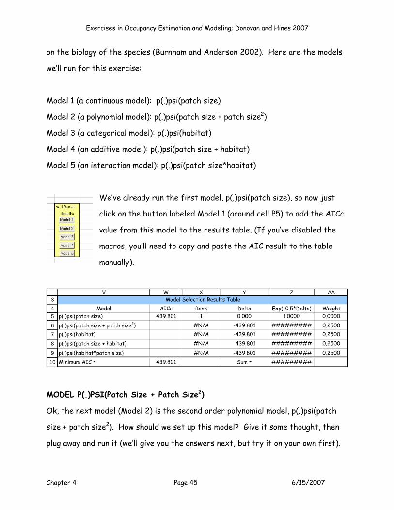
on the biology of the species (Burnham and Anderson 2002). Here are the models
we’ll run for this exercise:
Model 1 (a continuous model): p(.)psi(patch size)
Model 2 (a polynomial model): p(.)psi(patch size + patch size2)
Model 3 (a categorical model): p(.)psi(habitat)
Model 4 (an additive model): p(.)psi(patch size + habitat)
Model 5 (an interaction model): p(.)psi(patch size*habitat)
We’ve already run the first model, p(.)psi(patch size), so now just
click on the button labeled Model 1 (around cell P5) to add the AICc
value from this model to the results table. (If you’ve disabled the
macros, you’ll need to copy and paste the AIC result to the table
manually).
3
45
67
8
9
10
V W X Y Z AA
Model AICc Rank Delta Exp(-0.5*Delta) Weightp(.)psi(patch size) 439.801 1 0.000 1.0000 0.0000p(.)psi(patch size + patch size2) #N/A -439.801 ######### 0.2500p(.)psi(habitat) #N/A -439.801 ######### 0.2500
p(.)psi(patch size + habitat) #N/A -439.801 ######### 0.2500p(.)psi(habitat*patch size) #N/A -439.801 ######### 0.2500Minimum AIC = 439.801 Sum = #########
Model Selection Results Table
MODEL P(.)PSI(Patch Size + Patch Size2)
Ok, the next model (Model 2) is the second order polynomial model, p(.)psi(patch
size + patch size2). How should we set up this model? Give it some thought, then
plug away and run it (we’ll give you the answers next, but try it on your own first).
Exercises in Occupancy Estimation and Modeling; Donovan and Hines 2007
Chapter 4 Page 46 6/15/2007
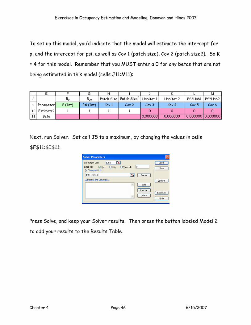
To set up this model, you’d indicate that the model will estimate the intercept for
p, and the intercept for psi, as well as Cov 1 (patch size), Cov 2 (patch size2). So K
= 4 for this model. Remember that you MUST enter a 0 for any betas that are not
being estimated in this model (cells J11:M11):
8
9
1011
E F G H I J K L MB0 B00 Patch Size Patch Size2 Habitat 1 Habitat 2 PS*Hab1 PS*Hab2
Parameter P (Int) Psi (Int) Cov 1 Cov 2 Cov 3 Cov 4 Cov 5 Cov 6Estimate? 1 1 1 1 0 0 0 0
Beta 0.000000 0.000000 0.000000 0.000000
Next, run Solver. Set cell J5 to a maximum, by changing the values in cells
$F$11:$I$11:
Press Solve, and keep your Solver results. Then press the button labeled Model 2
to add your results to the Results Table.
Exercises in Occupancy Estimation and Modeling; Donovan and Hines 2007
Chapter 4 Page 47 6/15/2007
3
45
67
8
9
10
V W X Y Z AA
Model AICc Rank Delta Exp(-0.5*Delta) Weightp(.)psi(patch size) 439.801 1 0.000 1.0000 0.0000p(.)psi(patch size + patch size2) 441.317 2 1.516 0.4686 0.0000p(.)psi(habitat) #N/A -439.801 ######### 0.3333
p(.)psi(patch size + habitat) #N/A -439.801 ######### 0.3333p(.)psi(habitat*patch size) #N/A -439.801 ######### 0.3333Minimum AIC = 439.801 Sum = #########
Model Selection Results Table
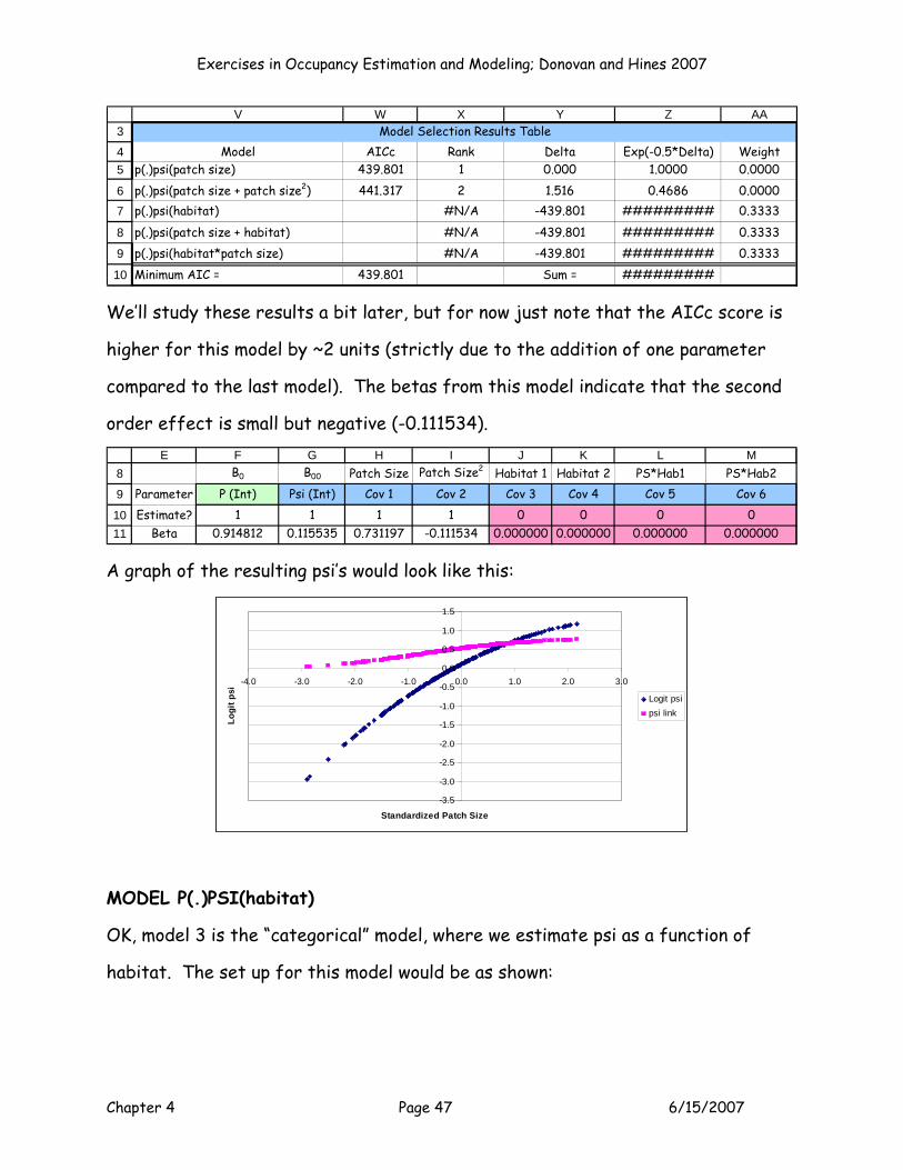
We’ll study these results a bit later, but for now just note that the AICc score is
higher for this model by ~2 units (strictly due to the addition of one parameter
compared to the last model). The betas from this model indicate that the second
order effect is small but negative (-0.111534).
8
9
1011
E F G H I J K L MB0 B00 Patch Size Patch Size2 Habitat 1 Habitat 2 PS*Hab1 PS*Hab2
Parameter P (Int) Psi (Int) Cov 1 Cov 2 Cov 3 Cov 4 Cov 5 Cov 6Estimate? 1 1 1 1 0 0 0 0
Beta 0.914812 0.115535 0.731197 -0.111534 0.000000 0.000000 0.000000 0.000000
A graph of the resulting psi’s would look like this:
-3.5
-3.0
-2.5
-2.0
-1.5
-1.0
-0.5
0.0
0.5
1.0
1.5
-4.0 -3.0 -2.0 -1.0 0.0 1.0 2.0 3.0
Standardized Patch Size
Logi
t psi
Logit psipsi link
MODEL P(.)PSI(habitat)
OK, model 3 is the “categorical” model, where we estimate psi as a function of
habitat. The set up for this model would be as shown:
Exercises in Occupancy Estimation and Modeling; Donovan and Hines 2007
Chapter 4 Page 48 6/15/2007
8
9
1011
E F G H I J K L MB0 B00 Patch Size Patch Size2 Habitat 1 Habitat 2 PS*Hab1 PS*Hab2
Parameter P (Int) Psi (Int) Cov 1 Cov 2 Cov 3 Cov 4 Cov 5 Cov 6Estimate? 1 1 0 0 1 1 0 0
Beta 0.000000 0.000000 0.000000 0.000000
Run this model by setting cell J5 to a maximum, by changing cells F11:G11, J11:K11.
Keep your Solver results, and then press the button labeled Model 3 to add your
results to the Results Table.
3
45
67
8
9
10
V W X Y Z AA
Model AICc Rank Delta Exp(-0.5*Delta) Weightp(.)psi(patch size) 439.801 1 0.000 1.0000 0.0000p(.)psi(patch size + patch size2) 441.317 2 1.516 0.4686 0.0000p(.)psi(habitat) 455.28361 3 15.482 0.0004 0.0000
p(.)psi(patch size + habitat) #N/A -439.801 ######### 0.5000p(.)psi(habitat*patch size) #N/A -439.801 ######### 0.5000Minimum AIC = 439.801 Sum = #########
Model Selection Results Table
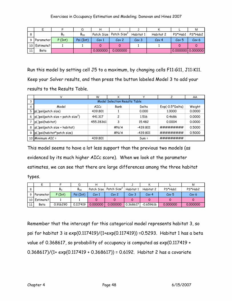
This model seems to have a lot less support than the previous two models (as
evidenced by its much higher AICc score). When we look at the parameter
estimates, we can see that there are large differences among the three habitat
types.
8
9
1011
E F G H I J K L MB0 B00 Patch Size Patch Size2 Habitat 1 Habitat 2 PS*Hab1 PS*Hab2
Parameter P (Int) Psi (Int) Cov 1 Cov 2 Cov 3 Cov 4 Cov 5 Cov 6Estimate? 1 1 0 0 0 0 0 0
Beta 0.916290 0.117419 0.000000 0.000000 0.368617 -0.659616 0.000000 0.000000
Remember that the intercept for this categorical model represents habitat 3, so
psi for habitat 3 is exp(0.117419)/(1+exp(0.117419)) =0.5293. Habitat 1 has a beta
value of 0.368617, so probability of occupancy is computed as exp(0.117419 +
0.368617)/(1+ exp(0.117419 + 0.368617)) = 0.6192. Habitat 2 has a covariate
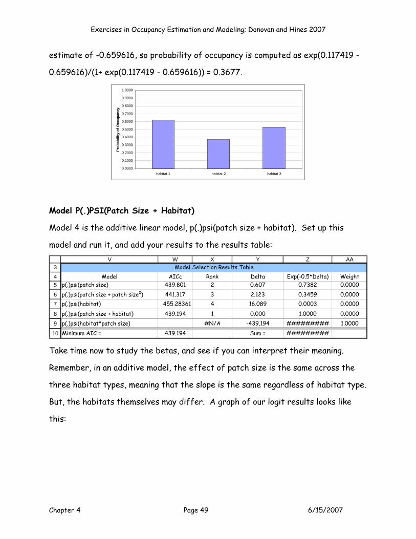
Exercises in Occupancy Estimation and Modeling; Donovan and Hines 2007
Chapter 4 Page 49 6/15/2007
estimate of -0.659616, so probability of occupancy is computed as exp(0.117419 -
0.659616)/(1+ exp(0.117419 - 0.659616)) = 0.3677.
0.0000
0.1000
0.2000
0.3000
0.4000
0.5000
0.6000
0.7000
0.8000
0.9000
1.0000
habitat 1 habitat 2 habitat 3
Pro
babi
lity
of O
ccup
ancy
Model P(.)PSI(Patch Size + Habitat)
Model 4 is the additive linear model, p(.)psi(patch size + habitat). Set up this
model and run it, and add your results to the results table:
3
45
67
8
9
10
V W X Y Z AA
Model AICc Rank Delta Exp(-0.5*Delta) Weightp(.)psi(patch size) 439.801 2 0.607 0.7382 0.0000p(.)psi(patch size + patch size2) 441.317 3 2.123 0.3459 0.0000p(.)psi(habitat) 455.28361 4 16.089 0.0003 0.0000
p(.)psi(patch size + habitat) 439.194 1 0.000 1.0000 0.0000p(.)psi(habitat*patch size) #N/A -439.194 ######### 1.0000Minimum AIC = 439.194 Sum = #########
Model Selection Results Table
Take time now to study the betas, and see if you can interpret their meaning.
Remember, in an additive model, the effect of patch size is the same across the
three habitat types, meaning that the slope is the same regardless of habitat type.
But, the habitats themselves may differ. A graph of our logit results looks like
this:
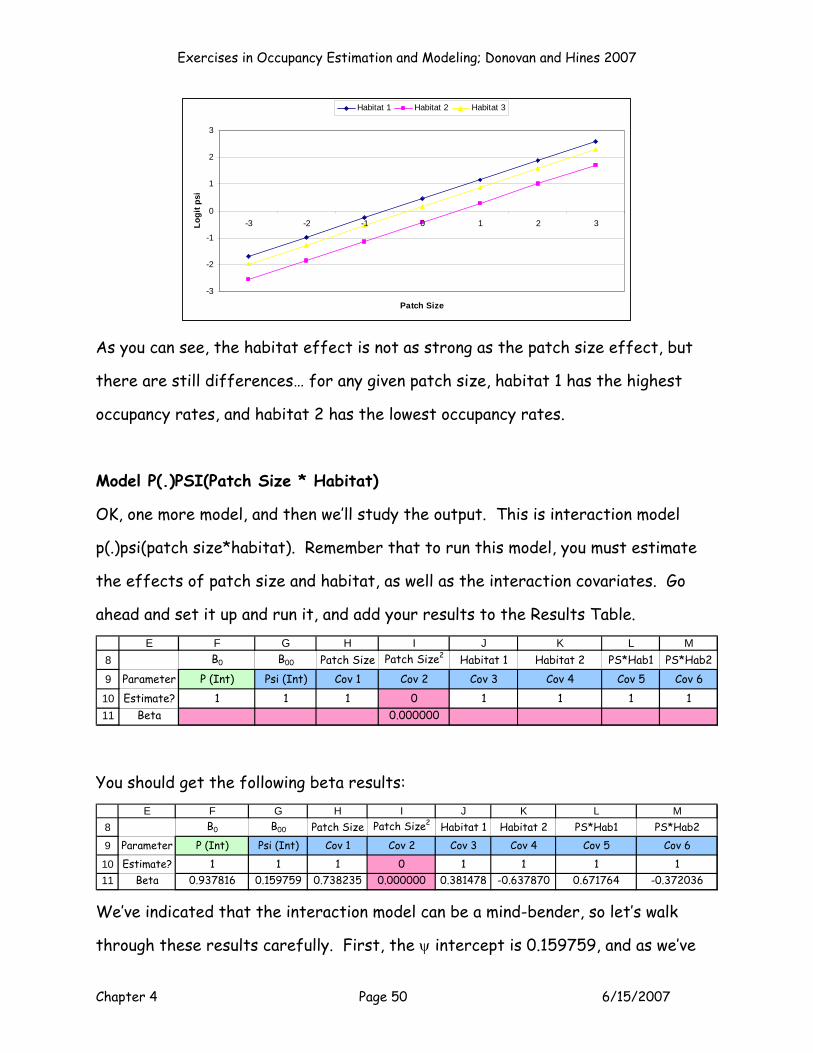
Exercises in Occupancy Estimation and Modeling; Donovan and Hines 2007
Chapter 4 Page 50 6/15/2007
-3
-2
-1
0
1
2
3
-3 -2 -1 0 1 2 3
Patch Size
Logi
t psi
Habitat 1 Habitat 2 Habitat 3
As you can see, the habitat effect is not as strong as the patch size effect, but
there are still differences… for any given patch size, habitat 1 has the highest
occupancy rates, and habitat 2 has the lowest occupancy rates.
Model P(.)PSI(Patch Size * Habitat)
OK, one more model, and then we’ll study the output. This is interaction model
p(.)psi(patch size*habitat). Remember that to run this model, you must estimate
the effects of patch size and habitat, as well as the interaction covariates. Go
ahead and set it up and run it, and add your results to the Results Table.
8
9
1011
E F G H I J K L MB0 B00 Patch Size Patch Size2 Habitat 1 Habitat 2 PS*Hab1 PS*Hab2
Parameter P (Int) Psi (Int) Cov 1 Cov 2 Cov 3 Cov 4 Cov 5 Cov 6Estimate? 1 1 1 0 1 1 1 1
Beta 0.000000
You should get the following beta results:
8
9
1011
E F G H I J K L MB0 B00 Patch Size Patch Size2 Habitat 1 Habitat 2 PS*Hab1 PS*Hab2
Parameter P (Int) Psi (Int) Cov 1 Cov 2 Cov 3 Cov 4 Cov 5 Cov 6Estimate? 1 1 1 0 1 1 1 1
Beta 0.937816 0.159759 0.738235 0.000000 0.381478 -0.637870 0.671764 -0.372036
We’ve indicated that the interaction model can be a mind-bender, so let’s walk
through these results carefully. First, the ψ intercept is 0.159759, and as we’ve
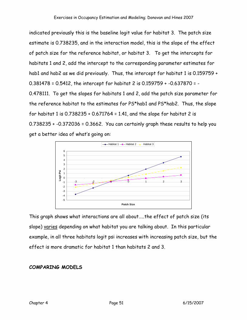
Exercises in Occupancy Estimation and Modeling; Donovan and Hines 2007
Chapter 4 Page 51 6/15/2007
indicated previously this is the baseline logit value for habitat 3. The patch size
estimate is 0.738235, and in the interaction model, this is the slope of the effect
of patch size for the reference habitat, or habitat 3. To get the intercepts for
habitats 1 and 2, add the intercept to the corresponding parameter estimates for
hab1 and hab2 as we did previously. Thus, the intercept for habitat 1 is 0.159759 +
0.381478 = 0.5412, the intercept for habitat 2 is 0.159759 + -0.637870 = -
0.478111. To get the slopes for habitats 1 and 2, add the patch size parameter for
the reference habitat to the estimates for PS*hab1 and PS*hab2. Thus, the slope
for habitat 1 is 0.738235 + 0.671764 = 1.41, and the slope for habitat 2 is
0.738235 + -0.372036 = 0.3662. You can certainly graph these results to help you
get a better idea of what’s going on:
-5
-4
-3
-2
-1
0
1
2
3
4
5
6
-3 -2 -1 0 1 2 3
Patch Size
Logi
t Psi
Habitat 1 Habitat 2 Habitat 3
This graph shows what interactions are all about…..the effect of patch size (its
slope) varies depending on what habitat you are talking about. In this particular
example, in all three habitats logit psi increases with increasing patch size, but the
effect is more dramatic for habitat 1 than habitats 2 and 3.
COMPARING MODELS
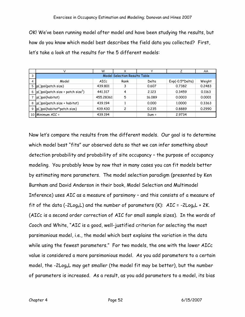
Exercises in Occupancy Estimation and Modeling; Donovan and Hines 2007
Chapter 4 Page 52 6/15/2007
OK! We’ve been running model after model and have been studying the results, but
how do you know which model best describes the field data you collected? First,
let’s take a look at the results for the 5 different models:
3
45
67
8
9
10
V W X Y Z AA
Model AICc Rank Delta Exp(-0.5*Delta) Weightp(.)psi(patch size) 439.801 3 0.607 0.7382 0.2483p(.)psi(patch size + patch size2) 441.317 4 2.123 0.3459 0.1163p(.)psi(habitat) 455.28361 5 16.089 0.0003 0.0001
p(.)psi(patch size + habitat) 439.194 1 0.000 1.0000 0.3363p(.)psi(habitat*patch size) 439.430 2 0.235 0.8889 0.2990Minimum AIC = 439.194 Sum = 2.9734
Model Selection Results Table
Now let’s compare the results from the different models. Our goal is to determine
which model best “fits” our observed data so that we can infer something about
detection probability and probability of site occupancy – the purpose of occupancy
modeling. You probably know by now that in many cases you can fit models better
by estimating more parameters. The model selection paradigm (presented by Ken
Burnham and David Anderson in their book, Model Selection and Multimodel
Inference) uses AIC as a measure of parsimony – and this consists of a measure of
fit of the data (-2LogeL) and the number of parameters (K): AIC = -2LogeL + 2K.
(AICc is a second order correction of AIC for small sample sizes). In the words of
Cooch and White, “AIC is a good, well-justified criterion for selecting the most
parsimonious model, i.e., the model which best explains the variation in the data
while using the fewest parameters.” For two models, the one with the lower AICc
value is considered a more parsimonious model. As you add parameters to a certain
model, the -2LogeL may get smaller (the model fit may be better), but the number
of parameters is increased. As a result, as you add parameters to a model, its bias
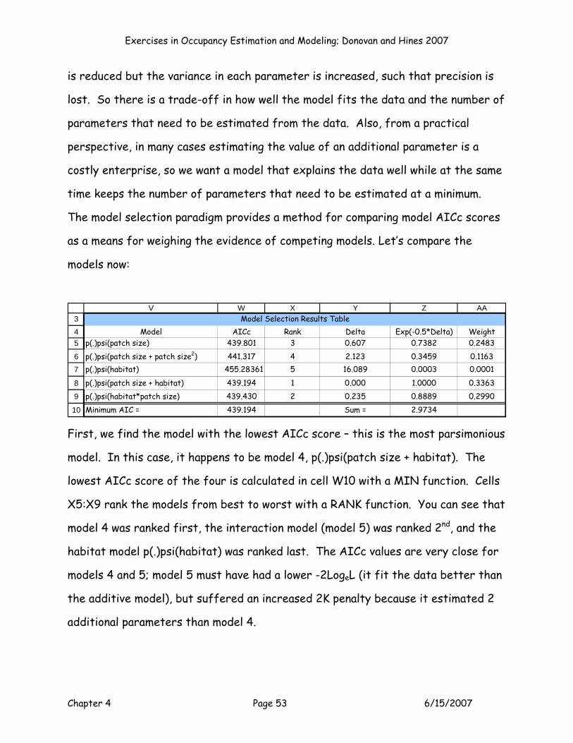
Exercises in Occupancy Estimation and Modeling; Donovan and Hines 2007
Chapter 4 Page 53 6/15/2007
is reduced but the variance in each parameter is increased, such that precision is
lost. So there is a trade-off in how well the model fits the data and the number of
parameters that need to be estimated from the data. Also, from a practical
perspective, in many cases estimating the value of an additional parameter is a
costly enterprise, so we want a model that explains the data well while at the same
time keeps the number of parameters that need to be estimated at a minimum.
The model selection paradigm provides a method for comparing model AICc scores
as a means for weighing the evidence of competing models. Let’s compare the
models now:
3
45
67
8
9
10
V W X Y Z AA
Model AICc Rank Delta Exp(-0.5*Delta) Weightp(.)psi(patch size) 439.801 3 0.607 0.7382 0.2483p(.)psi(patch size + patch size2) 441.317 4 2.123 0.3459 0.1163p(.)psi(habitat) 455.28361 5 16.089 0.0003 0.0001
p(.)psi(patch size + habitat) 439.194 1 0.000 1.0000 0.3363p(.)psi(habitat*patch size) 439.430 2 0.235 0.8889 0.2990Minimum AIC = 439.194 Sum = 2.9734
Model Selection Results Table
First, we find the model with the lowest AICc score – this is the most parsimonious
model. In this case, it happens to be model 4, p(.)psi(patch size + habitat). The
lowest AICc score of the four is calculated in cell W10 with a MIN function. Cells
X5:X9 rank the models from best to worst with a RANK function. You can see that
model 4 was ranked first, the interaction model (model 5) was ranked 2nd, and the
habitat model p(.)psi(habitat) was ranked last. The AICc values are very close for
models 4 and 5; model 5 must have had a lower -2LogeL (it fit the data better than
the additive model), but suffered an increased 2K penalty because it estimated 2
additional parameters than model 4.
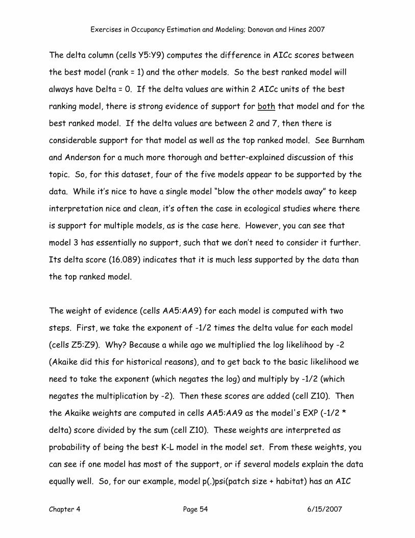
Exercises in Occupancy Estimation and Modeling; Donovan and Hines 2007
Chapter 4 Page 54 6/15/2007
The delta column (cells Y5:Y9) computes the difference in AICc scores between
the best model (rank = 1) and the other models. So the best ranked model will
always have Delta = 0. If the delta values are within 2 AICc units of the best
ranking model, there is strong evidence of support for both that model and for the
best ranked model. If the delta values are between 2 and 7, then there is
considerable support for that model as well as the top ranked model. See Burnham
and Anderson for a much more thorough and better-explained discussion of this
topic. So, for this dataset, four of the five models appear to be supported by the
data. While it’s nice to have a single model “blow the other models away” to keep
interpretation nice and clean, it’s often the case in ecological studies where there
is support for multiple models, as is the case here. However, you can see that
model 3 has essentially no support, such that we don’t need to consider it further.
Its delta score (16.089) indicates that it is much less supported by the data than
the top ranked model.
The weight of evidence (cells AA5:AA9) for each model is computed with two
steps. First, we take the exponent of -1/2 times the delta value for each model
(cells Z5:Z9). Why? Because a while ago we multiplied the log likelihood by -2
(Akaike did this for historical reasons), and to get back to the basic likelihood we
need to take the exponent (which negates the log) and multiply by -1/2 (which
negates the multiplication by -2). Then these scores are added (cell Z10). Then
the Akaike weights are computed in cells AA5:AA9 as the model's EXP (-1/2 *
delta) score divided by the sum (cell Z10). These weights are interpreted as
probability of being the best K-L model in the model set. From these weights, you
can see if one model has most of the support, or if several models explain the data
equally well. So, for our example, model p(.)psi(patch size + habitat) has an AIC
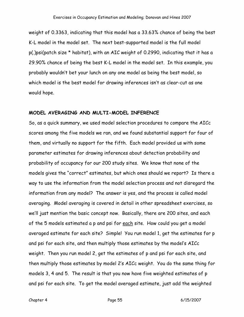
Exercises in Occupancy Estimation and Modeling; Donovan and Hines 2007
Chapter 4 Page 55 6/15/2007
weight of 0.3363, indicating that this model has a 33.63% chance of being the best
K-L model in the model set. The next best-supported model is the full model
p(.)psi(patch size * habitat), with an AIC weight of 0.2990, indicating that it has a
29.90% chance of being the best K-L model in the model set. In this example, you
probably wouldn’t bet your lunch on any one model as being the best model, so
which model is the best model for drawing inferences isn’t as clear-cut as one
would hope.
MODEL AVERAGING AND MULTI-MODEL INFERENCE
So, as a quick summary, we used model selection procedures to compare the AICc
scores among the five models we ran, and we found substantial support for four of
them, and virtually no support for the fifth. Each model provided us with some
parameter estimates for drawing inferences about detection probability and
probability of occupancy for our 200 study sites. We know that none of the
models gives the “correct” estimates, but which ones should we report? Is there a
way to use the information from the model selection process and not disregard the
information from any model? The answer is yes, and the process is called model
averaging. Model averaging is covered in detail in other spreadsheet exercises, so
we’ll just mention the basic concept now. Basically, there are 200 sites, and each
of the 5 models estimated a p and psi for each site. How could you get a model
averaged estimate for each site? Simple! You run model 1, get the estimates for p
and psi for each site, and then multiply those estimates by the model’s AICc
weight. Then you run model 2, get the estimates of p and psi for each site, and
then multiply those estimates by model 2’s AICc weight. You do the same thing for
models 3, 4 and 5. The result is that you now have five weighted estimates of p
and psi for each site. To get the model averaged estimate, just add the weighted

Exercises in Occupancy Estimation and Modeling; Donovan and Hines 2007
Chapter 4 Page 56 6/15/2007
estimates up…it’s that easy. However, estimating the standard errors of these
estimates is a bit more involved; see Cooch and White for more details.
TIME FOR A BREAK….
Ahhh! Much better!
ASSESSING MODEL FIT
OK. Hopefully you have some idea of how to run an occupancy model with
covariates, and how to compare among different models in a candidate set. We’ve
run five models, and were able to rank them and obtain their model weights.
However, we’ve missed a CRITICAL step – we haven’t assessed goodness of fit yet.
What if all 5 of the model’s we’ve run don’t really “fit” the data? Well, the model
selection procedures will still rank them from best to worst. If none of the models
fit the data, model selection procedures will simply rank a bunch of lousy models,
from the least lousy to the lousiest.
Until recently, a method of assessing goodness of fit for occupancy models was
lacking. Fortunately, Darryl MacKenzie and Larissa Bailey figured out a method for
assessing fit that is fairly straight-forward. The citation is: MacKenzie, D., and L.
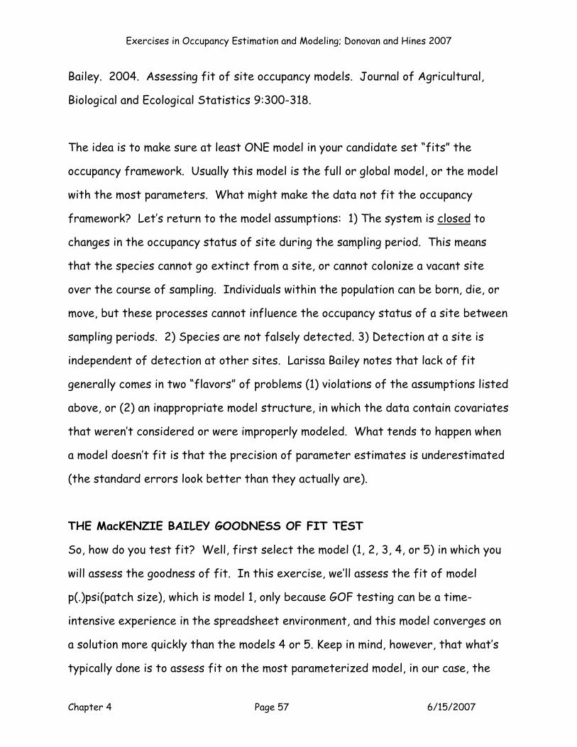
Exercises in Occupancy Estimation and Modeling; Donovan and Hines 2007
Chapter 4 Page 57 6/15/2007
Bailey. 2004. Assessing fit of site occupancy models. Journal of Agricultural,
Biological and Ecological Statistics 9:300-318.
The idea is to make sure at least ONE model in your candidate set “fits” the
occupancy framework. Usually this model is the full or global model, or the model
with the most parameters. What might make the data not fit the occupancy
framework? Let’s return to the model assumptions: 1) The system is closed to
changes in the occupancy status of site during the sampling period. This means
that the species cannot go extinct from a site, or cannot colonize a vacant site
over the course of sampling. Individuals within the population can be born, die, or
move, but these processes cannot influence the occupancy status of a site between
sampling periods. 2) Species are not falsely detected. 3) Detection at a site is
independent of detection at other sites. Larissa Bailey notes that lack of fit
generally comes in two “flavors” of problems (1) violations of the assumptions listed
above, or (2) an inappropriate model structure, in which the data contain covariates
that weren’t considered or were improperly modeled. What tends to happen when
a model doesn’t fit is that the precision of parameter estimates is underestimated
(the standard errors look better than they actually are).
THE MacKENZIE BAILEY GOODNESS OF FIT TEST
So, how do you test fit? Well, first select the model (1, 2, 3, 4, or 5) in which you
will assess the goodness of fit. In this exercise, we’ll assess the fit of model
p(.)psi(patch size), which is model 1, only because GOF testing can be a time-
intensive experience in the spreadsheet environment, and this model converges on
a solution more quickly than the models 4 or 5. Keep in mind, however, that what’s
typically done is to assess fit on the most parameterized model, in our case, the
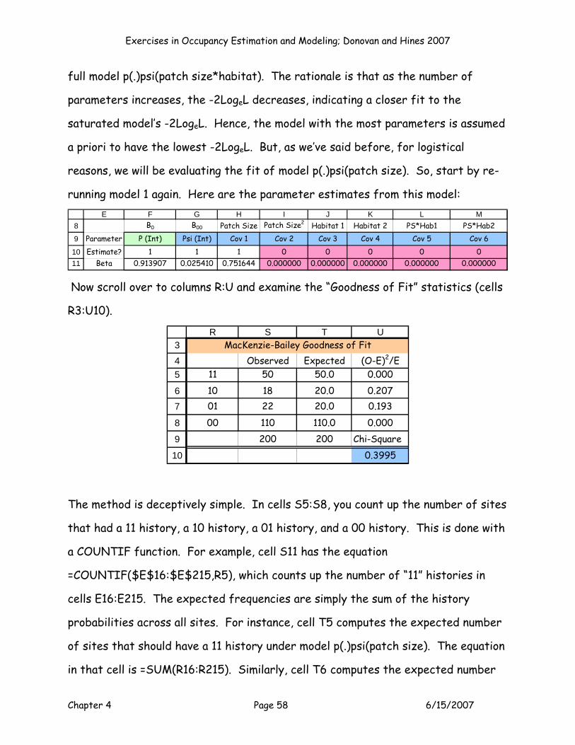
Exercises in Occupancy Estimation and Modeling; Donovan and Hines 2007
Chapter 4 Page 58 6/15/2007
full model p(.)psi(patch size*habitat). The rationale is that as the number of
parameters increases, the -2LogeL decreases, indicating a closer fit to the
saturated model’s -2LogeL. Hence, the model with the most parameters is assumed
a priori to have the lowest -2LogeL. But, as we’ve said before, for logistical
reasons, we will be evaluating the fit of model p(.)psi(patch size). So, start by re-
running model 1 again. Here are the parameter estimates from this model:
8
9
1011
E F G H I J K L MB0 B00 Patch Size Patch Size2 Habitat 1 Habitat 2 PS*Hab1 PS*Hab2
Parameter P (Int) Psi (Int) Cov 1 Cov 2 Cov 3 Cov 4 Cov 5 Cov 6Estimate? 1 1 1 0 0 0 0 0
Beta 0.913907 0.025410 0.751644 0.000000 0.000000 0.000000 0.000000 0.000000
Now scroll over to columns R:U and examine the “Goodness of Fit” statistics (cells
R3:U10).
3
45
67
8
9
10
R S T U
Observed Expected (O-E)2/E11 50 50.0 0.00010 18 20.0 0.20701 22 20.0 0.193
00 110 110.0 0.000200 200 Chi-Square
0.3995
MacKenzie-Bailey Goodness of Fit
The method is deceptively simple. In cells S5:S8, you count up the number of sites
that had a 11 history, a 10 history, a 01 history, and a 00 history. This is done with
a COUNTIF function. For example, cell S11 has the equation
=COUNTIF($E$16:$E$215,R5), which counts up the number of “11” histories in
cells E16:E215. The expected frequencies are simply the sum of the history
probabilities across all sites. For instance, cell T5 computes the expected number
of sites that should have a 11 history under model p(.)psi(patch size). The equation
in that cell is =SUM(R16:R215). Similarly, cell T6 computes the expected number
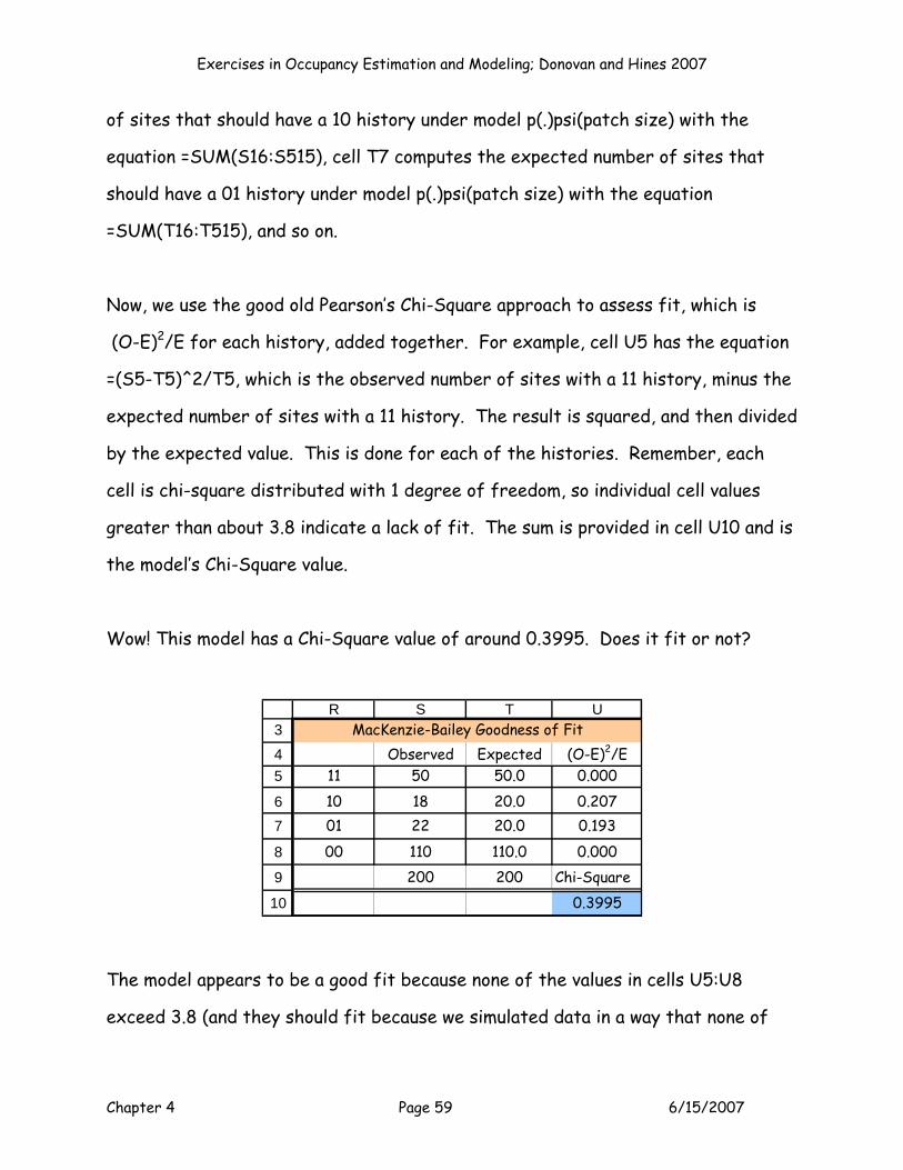
Exercises in Occupancy Estimation and Modeling; Donovan and Hines 2007
Chapter 4 Page 59 6/15/2007
of sites that should have a 10 history under model p(.)psi(patch size) with the
equation =SUM(S16:S515), cell T7 computes the expected number of sites that
should have a 01 history under model p(.)psi(patch size) with the equation
=SUM(T16:T515), and so on.
Now, we use the good old Pearson’s Chi-Square approach to assess fit, which is
(O-E)2/E for each history, added together. For example, cell U5 has the equation
=(S5-T5)^2/T5, which is the observed number of sites with a 11 history, minus the
expected number of sites with a 11 history. The result is squared, and then divided
by the expected value. This is done for each of the histories. Remember, each
cell is chi-square distributed with 1 degree of freedom, so individual cell values
greater than about 3.8 indicate a lack of fit. The sum is provided in cell U10 and is
the model’s Chi-Square value.
Wow! This model has a Chi-Square value of around 0.3995. Does it fit or not?
3
45
67
8
9
10
R S T U
Observed Expected (O-E)2/E11 50 50.0 0.00010 18 20.0 0.20701 22 20.0 0.193
00 110 110.0 0.000200 200 Chi-Square
0.3995
MacKenzie-Bailey Goodness of Fit
The model appears to be a good fit because none of the values in cells U5:U8
exceed 3.8 (and they should fit because we simulated data in a way that none of

Exercises in Occupancy Estimation and Modeling; Donovan and Hines 2007
Chapter 4 Page 60 6/15/2007
the model assumptions were violated). And if this model fits (which is ranked third
out of five models), the top two models in the model set should fit as well.
THE BOOTSTRAP
But let’s suppose that the chi square value was a lot higher. How would you know
whether to conclude the data fit or not? Well, currently the best way to test “fit”
is to simulate a new dataset (called a bootstrap dataset) based on the parameter
estimates (betas) from the model you are assessing (model 1: p(.)psi(patch size)).
Here are the steps we’ll be using to assess fit with a bootstrap, as specified by
MacKenzie and Bailey:
1. Run model p(.)psi(patch size) and obtain beta estimates and the Pearson Chi-
Square test statistic.
2. Use those beta estimates to simulate a bootstrap dataset (i.e., generate new
encounter histories for each site – the covariates for each site are the same
as the original data).
3. Once you have a simulated bootstrap dataset, then run the analysis again,
and compute the Pearson Chi Square test statistic and store it. Because you
simulated the data based on the results from an actual model, you KNOW
the simulated data fit will fit the model.
4. Repeat the process about 1000 times.
5. Take all 1000 bootstrap Chi-Square results, order them, and find out where
your model’s Chi-Square (calculated from the real data) value falls within
this bootstrap distribution. It sounds like a lot of work, but it’s not really if
you use a macro in the spreadsheet to run your trials for you. Plus, MARK
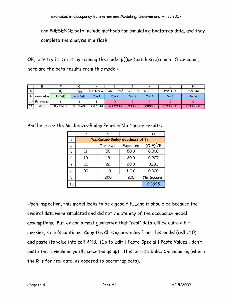
Exercises in Occupancy Estimation and Modeling; Donovan and Hines 2007
Chapter 4 Page 61 6/15/2007
and PRESENCE both include methods for simulating bootstrap data, and they
complete the analysis in a flash.
OK, let’s try it. Start by running the model p(.)psi(patch size) again. Once again,
here are the beta results from this model:
8
9
1011
E F G H I J K L MB0 B00 Patch Size Patch Size2 Habitat 1 Habitat 2 PS*Hab1 PS*Hab2
Parameter P (Int) Psi (Int) Cov 1 Cov 2 Cov 3 Cov 4 Cov 5 Cov 6Estimate? 1 1 1 0 0 0 0 0
Beta 0.913907 0.025410 0.751644 0.000000 0.000000 0.000000 0.000000 0.000000
And here are the MacKenzie-Bailey Pearson Chi Square results:
3
45
67
8
9
10
R S T U
Observed Expected (O-E)2/E11 50 50.0 0.00010 18 20.0 0.20701 22 20.0 0.193
00 110 110.0 0.000200 200 Chi-Square
0.3995
MacKenzie-Bailey Goodness of Fit
Upon inspection, this model looks to be a good fit…..and it should be because the
original data were simulated and did not violate any of the occupancy model
assumptions. But we can almost guarantee that “real” data will be quite a bit
messier, so let’s continue. Copy the Chi-Square value from this model (cell U10)
and paste its value into cell AN8. (Go to Edit | Paste Special | Paste Values….don’t
paste the formula or you’ll screw things up). This cell is labeled Chi-SquareR (where
the R is for real data, as opposed to bootstrap data).
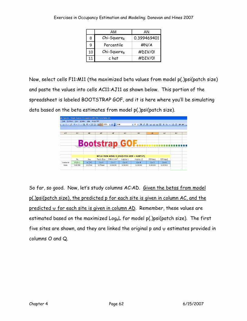
Exercises in Occupancy Estimation and Modeling; Donovan and Hines 2007
Chapter 4 Page 62 6/15/2007
8
9
1011
AM ANChi-SquareR 0.399469401Percentile #N/A
Chi-SquareB #DIV/0!c hat #DIV/0!
Now, select cells F11:M11 (the maximized beta values from model p(.)psi(patch size)
and paste the values into cells AC11:AJ11 as shown below. This portion of the
spreadsheet is labeled BOOTSTRAP GOF, and it is here where you’ll be simulating
data based on the beta estimates from model p(.)psi(patch size).
So far, so good. Now, let’s study columns AC:AD. Given the betas from model
p(.)psi(patch size), the predicted p for each site is given in column AC, and the
predicted ψ for each site is given in column AD. Remember, these values are
estimated based on the maximized LogeL for model p(.)psi(patch size). The first
five sites are shown, and they are linked the original p and ψ estimates provided in
columns O and Q.
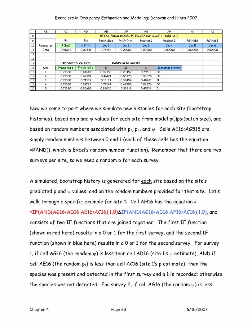
Exercises in Occupancy Estimation and Modeling; Donovan and Hines 2007
Chapter 4 Page 63 6/15/2007
8
9
1011121314151617181920
AB AC AD AE AF AG AH AI AJ
B0 B00 Patch Size Patch Size2 Habitat 1 Habitat 2 PS*Hab1 PS*Hab2Parameter P (Int) ψ (Int) Cov 1 Cov 2 Cov 3 Cov 4 Cov 5 Cov 6
Beta 0.91391 0.02541 0.75164 0.00000 0.00000 0.00000 0.00000 0.00000
Site Predicted p Predicted ψ p1 p2 ψ Bootstrap History1 0.71380 0.18648 0.07352 0.23457 0.79512 002 0.71380 0.67951 0.46121 0.86373 0.93078 003 0.71380 0.71339 0.13123 0.32454 0.48481 114 0.71380 0.19792 0.77144 0.47305 0.98876 005 0.71380 0.70693 0.88030 0.33814 0.41534 01
PREDICTED VALUES RANDOM NUMBERS
BETAS FROM MODEL P(.)PSI(PATCH SIZE + HABITAT)
Now we come to part where we simulate new histories for each site (bootstrap
histories), based on p and ψ values for each site from model p(.)psi(patch size), and
based on random numbers associated with p1, p2, and ψ. Cells AE16:AG515 are
simply random numbers between 0 and 1 (each of these cells has the equation
=RAND(), which is Excel’s random number function). Remember that there are two
surveys per site, so we need a random p for each survey.
A simulated, bootstrap history is generated for each site based on the site’s
predicted p and ψ values, and on the random numbers provided for that site. Let’s
walk through a specific example for site 1: Cell AH16 has the equation =
=IF(AND(AG16<AD16,AE16<AC16),1,0)&IF(AND(AG16<AD16,AF16<AC16),1,0), and
consists of two IF functions that are joined together. The first IF function
(shown in red here) results in a 0 or 1 for the first survey, and the second IF
function (shown in blue here) results in a 0 or 1 for the second survey. For survey
1, if cell AG16 (the random ψ) is less than cell AD16 (site 1’s ψ estimate), AND if
cell AE16 (the random p1) is less than cell AC16 (site 1’s p estimate), then the
species was present and detected in the first survey and a 1 is recorded; otherwise
the species was not detected. For survey 2, if cell AG16 (the random ψ) is less

Exercises in Occupancy Estimation and Modeling; Donovan and Hines 2007
Chapter 4 Page 64 6/15/2007
than cell AD16 (site 1’s ψ estimate), AND if cell AF16 (the random p2) is less than
cell AC16 (site 1’s p estimate), then the species was present and detected in the
first survey and a 1 is recorded; otherwise the species was either not present, and
thus not detected, or was simply not detected even though the site was occupied.
This formula is copied down for all 200 sites, and provides us with a “bootstrapped
histories” for each site. What’s the big deal? Well, because we used random
numbers to simulate histories, we know that we have not violated any of the
occupancy model assumptions, namely: 1) The system is demographically closed to
changes in the occupancy status of site during the sampling period – we used the
same ψ value for both surveys so there was no change in occupancy pattern. 2)
Species are not falsely detected – we either detected the species or not based on
the random number for each survey, and there were no mistakes in data recording
that would change a 0 1 or 1 0. 3) Detection at a site is independent of
detection at other sites – each site has its own random numbers and in no way does
a random number for one site influence the random number associated with
another site. We also know that there are no structural problems with the data
because we simulated data based on a model with specified covariates, and we
analyzed the data with the exact same model structure. In short, the simulated
data are known to fit.
Notice when you press F9, the calculate key, Excel generates new random numbers,
and hence new bootstrapped histories. Let’s take a look at the first three sites
shown below and determine how they ended up with 00, 11, and 10 histories,
respectively.
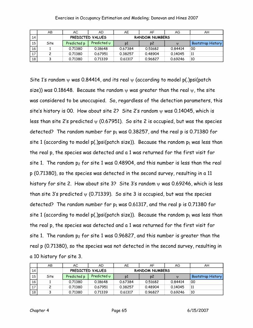
Exercises in Occupancy Estimation and Modeling; Donovan and Hines 2007
Chapter 4 Page 65 6/15/2007
1415161718
AB AC AD AE AF AG AH
Site Predicted p Predicted ψ p1 p2 ψ Bootstrap History1 0.71380 0.18648 0.67384 0.51682 0.84414 002 0.71380 0.67951 0.38257 0.48904 0.14045 113 0.71380 0.71339 0.61317 0.96827 0.69246 10
PREDICTED VALUES RANDOM NUMBERS
Site 1’s random ψ was 0.84414, and its real ψ (according to model p(.)psi(patch
size)) was 0.18648. Because the random ψ was greater than the real ψ, the site
was considered to be unoccupied. So, regardless of the detection parameters, this
site’s history is 00. How about site 2? Site 2’s random ψ was 0.14045, which is
less than site 2’s predicted ψ (0.67951). So site 2 is occupied, but was the species
detected? The random number for p1 was 0.38257, and the real p is 0.71380 for
site 1 (according to model p(.)psi(patch size)). Because the random p1 was less than
the real p, the species was detected and a 1 was returned for the first visit for
site 1. The random p2 for site 1 was 0.48904, and this number is less than the real
p (0.71380), so the species was detected in the second survey, resulting in a 11
history for site 2. How about site 3? Site 3’s random ψ was 0.69246, which is less
than site 3’s predicted ψ (0.71339). So site 3 is occupied, but was the species
detected? The random number for p1 was 0.61317, and the real p is 0.71380 for
site 1 (according to model p(.)psi(patch size)). Because the random p1 was less than
the real p, the species was detected and a 1 was returned for the first visit for
site 1. The random p2 for site 1 was 0.96827, and this number is greater than the
real p (0.71380), so the species was not detected in the second survey, resulting in
a 10 history for site 3.
1415161718
AB AC AD AE AF AG AH
Site Predicted p Predicted ψ p1 p2 ψ Bootstrap History1 0.71380 0.18648 0.67384 0.51682 0.84414 002 0.71380 0.67951 0.38257 0.48904 0.14045 113 0.71380 0.71339 0.61317 0.96827 0.69246 10
PREDICTED VALUES RANDOM NUMBERS
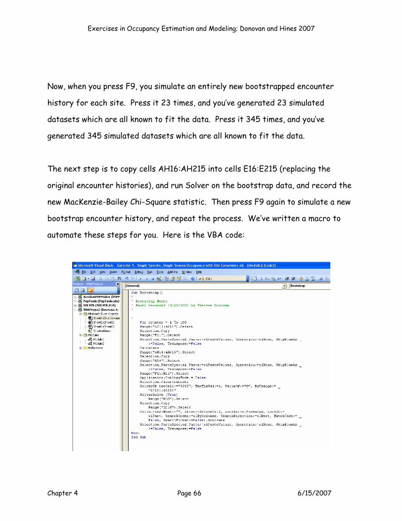
Exercises in Occupancy Estimation and Modeling; Donovan and Hines 2007
Chapter 4 Page 66 6/15/2007
Now, when you press F9, you simulate an entirely new bootstrapped encounter
history for each site. Press it 23 times, and you’ve generated 23 simulated
datasets which are all known to fit the data. Press it 345 times, and you’ve
generated 345 simulated datasets which are all known to fit the data.
The next step is to copy cells AH16:AH215 into cells E16:E215 (replacing the
original encounter histories), and run Solver on the bootstrap data, and record the
new MacKenzie-Bailey Chi-Square statistic. Then press F9 again to simulate a new
bootstrap encounter history, and repeat the process. We’ve written a macro to
automate these steps for you. Here is the VBA code:

Exercises in Occupancy Estimation and Modeling; Donovan and Hines 2007
Chapter 4 Page 67 6/15/2007
Just press the little smiley face and you’ll run this code 100 times, representing
100 bootstrap trials. You can run more or fewer trials if you’d like, just go to
Macros | Boostrap | Edit, and change the code
For counter = 1 to 100 to For counter = 1 to X (and replace the X with
whatever number you’d like). Then, close out of the visual basic editor. Ideally,
you’d run 1,000 or even 10,000 trials, but that’s beyond our purpose here.
Important note: If you can’t get the bootstrap to run, here’s what you should try first: Go to Tools | Macro | Macros | Bootstrap | Edit. Then, with the Visual Basic module active, click References on the Tools menu, and then select the Solver.xla check box under Available References. If Solver.xla doesn't appear under Available References, click Browse and open Solver.xla in the \Office\Library\Solver\ subfolder. *************************************************************************
Go ahead and press the smiley face – this might be a good time to go grab some
lunch – the spreadsheet is very slow compared to MARK or PRESENCE. After the
100 trails are completed, take a good look the bootstrap results in columns AL:AN.
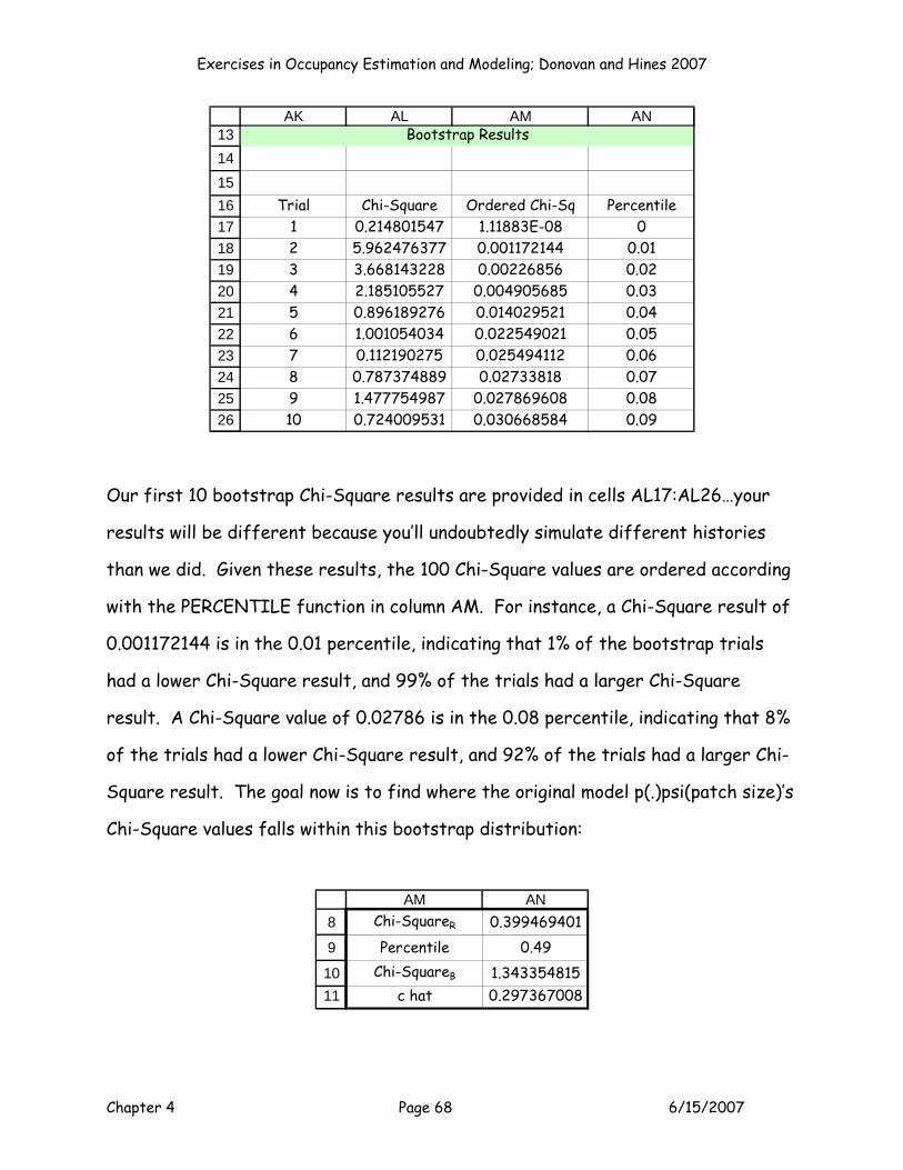
Exercises in Occupancy Estimation and Modeling; Donovan and Hines 2007
Chapter 4 Page 68 6/15/2007
1314151617181920212223242526
AK AL AM AN
Trial Chi-Square Ordered Chi-Sq Percentile1 0.214801547 1.11883E-08 02 5.962476377 0.001172144 0.013 3.668143228 0.00226856 0.024 2.185105527 0.004905685 0.035 0.896189276 0.014029521 0.046 1.001054034 0.022549021 0.057 0.112190275 0.025494112 0.068 0.787374889 0.02733818 0.079 1.477754987 0.027869608 0.0810 0.724009531 0.030668584 0.09
Bootstrap Results
Our first 10 bootstrap Chi-Square results are provided in cells AL17:AL26…your
results will be different because you’ll undoubtedly simulate different histories
than we did. Given these results, the 100 Chi-Square values are ordered according
with the PERCENTILE function in column AM. For instance, a Chi-Square result of
0.001172144 is in the 0.01 percentile, indicating that 1% of the bootstrap trials
had a lower Chi-Square result, and 99% of the trials had a larger Chi-Square
result. A Chi-Square value of 0.02786 is in the 0.08 percentile, indicating that 8%
of the trials had a lower Chi-Square result, and 92% of the trials had a larger Chi-
Square result. The goal now is to find where the original model p(.)psi(patch size)’s
Chi-Square values falls within this bootstrap distribution:
8
9
1011
AM ANChi-SquareR 0.399469401Percentile 0.49
Chi-SquareB 1.343354815c hat 0.297367008
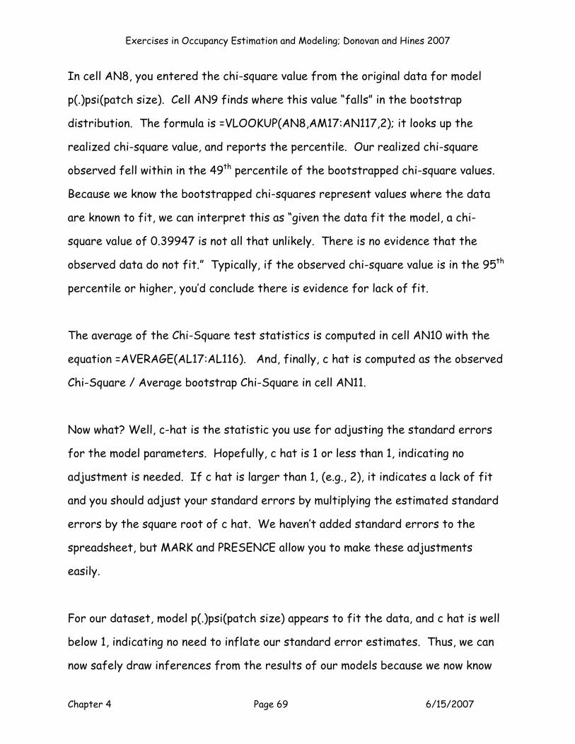
Exercises in Occupancy Estimation and Modeling; Donovan and Hines 2007
Chapter 4 Page 69 6/15/2007
In cell AN8, you entered the chi-square value from the original data for model
p(.)psi(patch size). Cell AN9 finds where this value “falls” in the bootstrap
distribution. The formula is =VLOOKUP(AN8,AM17:AN117,2); it looks up the
realized chi-square value, and reports the percentile. Our realized chi-square
observed fell within in the 49th percentile of the bootstrapped chi-square values.
Because we know the bootstrapped chi-squares represent values where the data
are known to fit, we can interpret this as “given the data fit the model, a chi-
square value of 0.39947 is not all that unlikely. There is no evidence that the
observed data do not fit.” Typically, if the observed chi-square value is in the 95th
percentile or higher, you’d conclude there is evidence for lack of fit.
The average of the Chi-Square test statistics is computed in cell AN10 with the
equation =AVERAGE(AL17:AL116). And, finally, c hat is computed as the observed
Chi-Square / Average bootstrap Chi-Square in cell AN11.
Now what? Well, c-hat is the statistic you use for adjusting the standard errors
for the model parameters. Hopefully, c hat is 1 or less than 1, indicating no
adjustment is needed. If c hat is larger than 1, (e.g., 2), it indicates a lack of fit
and you should adjust your standard errors by multiplying the estimated standard
errors by the square root of c hat. We haven’t added standard errors to the
spreadsheet, but MARK and PRESENCE allow you to make these adjustments
easily.
For our dataset, model p(.)psi(patch size) appears to fit the data, and c hat is well
below 1, indicating no need to inflate our standard error estimates. Thus, we can
now safely draw inferences from the results of our models because we now know
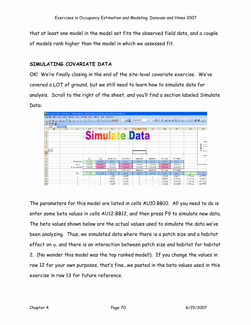
Exercises in Occupancy Estimation and Modeling; Donovan and Hines 2007
Chapter 4 Page 70 6/15/2007
that at least one model in the model set fits the observed field data, and a couple
of models rank higher than the model in which we assessed fit.
SIMULATING COVARIATE DATA
OK! We’re finally closing in the end of the site-level covariate exercise. We’ve
covered a LOT of ground, but we still need to learn how to simulate data for
analysis. Scroll to the right of the sheet, and you’ll find a section labeled Simulate
Data:
The parameters for this model are listed in cells AU10:BB10. All you need to do is
enter some beta values in cells AU12:BB12, and then press F9 to simulate new data.
The beta values shown below are the actual values used to simulate the data we’ve
been analyzing. Thus, we simulated data where there is a patch size and a habitat
effect on ψ, and there is an interaction between patch size and habitat for habitat
2. (No wonder this model was the top ranked model!). If you change the values in
row 12 for your own purposes, that’s fine…we pasted in the beta values used in this
exercise in row 13 for future reference.
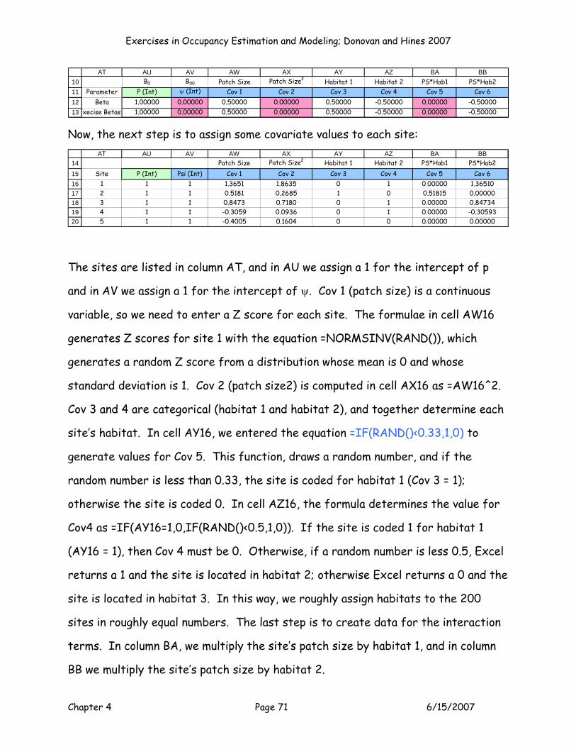
Exercises in Occupancy Estimation and Modeling; Donovan and Hines 2007
Chapter 4 Page 71 6/15/2007
10111213
AT AU AV AW AX AY AZ BA BBB0 B00 Patch Size Patch Size2 Habitat 1 Habitat 2 PS*Hab1 PS*Hab2
Parameter P (Int) ψ (Int) Cov 1 Cov 2 Cov 3 Cov 4 Cov 5 Cov 6Beta 1.00000 0.00000 0.50000 0.00000 0.50000 -0.50000 0.00000 -0.50000
Execise Betas 1.00000 0.00000 0.50000 0.00000 0.50000 -0.50000 0.00000 -0.50000
Now, the next step is to assign some covariate values to each site:
14151617181920
AT AU AV AW AX AY AZ BA BBPatch Size Patch Size2 Habitat 1 Habitat 2 PS*Hab1 PS*Hab2
Site P (Int) Psi (Int) Cov 1 Cov 2 Cov 3 Cov 4 Cov 5 Cov 61 1 1 1.3651 1.8635 0 1 0.00000 1.365102 1 1 0.5181 0.2685 1 0 0.51815 0.000003 1 1 0.8473 0.7180 0 1 0.00000 0.847344 1 1 -0.3059 0.0936 0 1 0.00000 -0.305935 1 1 -0.4005 0.1604 0 0 0.00000 0.00000
The sites are listed in column AT, and in AU we assign a 1 for the intercept of p
and in AV we assign a 1 for the intercept of ψ. Cov 1 (patch size) is a continuous
variable, so we need to enter a Z score for each site. The formulae in cell AW16
generates Z scores for site 1 with the equation =NORMSINV(RAND()), which
generates a random Z score from a distribution whose mean is 0 and whose
standard deviation is 1. Cov 2 (patch size2) is computed in cell AX16 as =AW16^2.
Cov 3 and 4 are categorical (habitat 1 and habitat 2), and together determine each
site’s habitat. In cell AY16, we entered the equation =IF(RAND()<0.33,1,0) to
generate values for Cov 5. This function, draws a random number, and if the
random number is less than 0.33, the site is coded for habitat 1 (Cov 3 = 1);
otherwise the site is coded 0. In cell AZ16, the formula determines the value for
Cov4 as =IF(AY16=1,0,IF(RAND()<0.5,1,0)). If the site is coded 1 for habitat 1
(AY16 = 1), then Cov 4 must be 0. Otherwise, if a random number is less 0.5, Excel
returns a 1 and the site is located in habitat 2; otherwise Excel returns a 0 and the
site is located in habitat 3. In this way, we roughly assign habitats to the 200
sites in roughly equal numbers. The last step is to create data for the interaction
terms. In column BA, we multiply the site’s patch size by habitat 1, and in column
BB we multiply the site’s patch size by habitat 2.
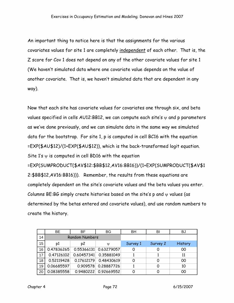
Exercises in Occupancy Estimation and Modeling; Donovan and Hines 2007
Chapter 4 Page 72 6/15/2007
An important thing to notice here is that the assignments for the various
covariates values for site 1 are completely independent of each other. That is, the
Z score for Cov 1 does not depend on any of the other covariate values for site 1
(We haven’t simulated data where one covariate value depends on the value of
another covariate. That is, we haven’t simulated data that are dependent in any
way).
Now that each site has covariate values for covariates one through six, and beta
values specified in cells AU12:BB12, we can compute each site’s ψ and p parameters
as we’ve done previously, and we can simulate data in the same way we simulated
data for the bootstrap. For site 1, p is computed in cell BC16 with the equation
=EXP($AU$12)/(1+EXP($AU$12)), which is the back-transformed logit equation.
Site 1’s ψ is computed in cell BD16 with the equation
=EXP(SUMPRODUCT($AV$12:$BB$12,AV16:BB16))/(1+EXP(SUMPRODUCT($AV$1
2:$BB$12,AV16:BB16))). Remember, the results from these equations are
completely dependent on the site’s covariate values and the beta values you enter.
Columns BE:BG simply create histories based on the site’s p and ψ values (as
determined by the betas entered and covariate values), and use random numbers to
create the history.
14151617181920
BE BF BG BH BI BJ
p1 p2 ψ Survey 1 Survey 2 History0.47836265 0.55366131 0.63279057 0 0 000.47126102 0.60457341 0.35881049 1 1 110.52119428 0.17612179 0.48430619 0 0 00
0.06685597 0.909578 0.28887726 1 0 100.08385558 0.9480222 0.92669552 0 0 00
Random Numbers
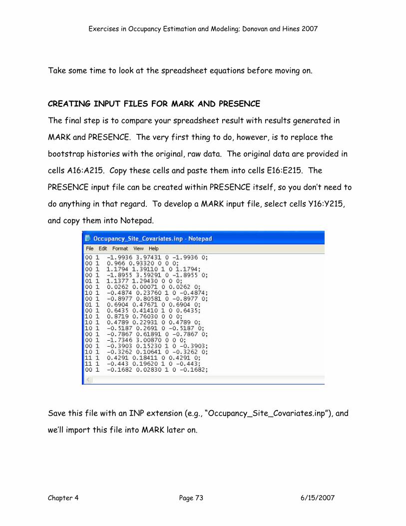
Exercises in Occupancy Estimation and Modeling; Donovan and Hines 2007
Chapter 4 Page 73 6/15/2007
Take some time to look at the spreadsheet equations before moving on.
CREATING INPUT FILES FOR MARK AND PRESENCE
The final step is to compare your spreadsheet result with results generated in
MARK and PRESENCE. The very first thing to do, however, is to replace the
bootstrap histories with the original, raw data. The original data are provided in
cells A16:A215. Copy these cells and paste them into cells E16:E215. The
PRESENCE input file can be created within PRESENCE itself, so you don’t need to
do anything in that regard. To develop a MARK input file, select cells Y16:Y215,
and copy them into Notepad.
Save this file with an INP extension (e.g., “Occupancy_Site_Covariates.inp”), and
we’ll import this file into MARK later on.
Exercises in Occupancy Estimation and Modeling; Donovan and Hines 2007
Chapter 4 Page 74 6/15/2007
SINGLE-SPECIES, SINGLE-SEASON OCCUPANCY WITH SITE
COVARIATES IN PROGRAM PRESENCE
INPUT DATA
In this exercise, we will analyze the data in the spreadsheet Site Covariates in
program PRESENCE. Recall that there are no detection covariates, and that there
are several site-level covariates (patch size, patch size2, two habitat covariates
that code for three habitat types, as well as the two covariates for the patch size
by habitat interactions), making a total of 6 covariates. Remember that this
worksheet has only two sampling sessions. Before you begin, make sure that the
data you are working with are the original data. That is, make sure the histories in
column E match those in column A. If they don’t match, copy the histories in
column A into column E, using the Paste Special | Paste Values option.
Open PRESENCE and go to File | New. In the Enter Specifications Form, we’ll
create the PRESENCE input file. Enter a title for the analysis (e.g., Single-Season
Occupancy with Site Covariates). Enter 200 for the number of sites, and 2 for the
number of occasions. Again, in this particular dataset, all of the covariates (n = 6)
are considered site level covariates.

Exercises in Occupancy Estimation and Modeling; Donovan and Hines 2007
Chapter 4 Page 75 6/15/2007
When you are finished, click on the Input Data Form. PRESENCE then presents
you with the Data Input Form, where you can paste in your data. Notice that there
are two tabs on the form: Presence/Absence Data and Site Covars. First, we’ll
paste in the encounter histories in the tab labeled Presence/Absence Data. On
your spreadsheet, select C16:D215 and go to Edit | Copy. Then go to the Data
Input Form, select the first box and select Edit | Paste, and select the Paste
Values option.
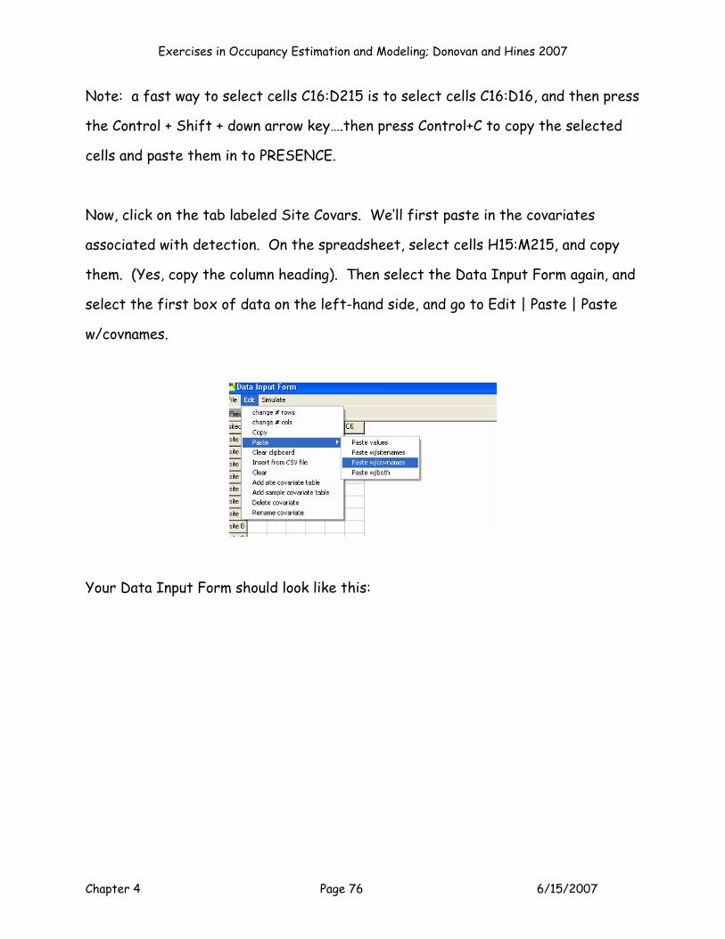
Exercises in Occupancy Estimation and Modeling; Donovan and Hines 2007
Chapter 4 Page 76 6/15/2007
Note: a fast way to select cells C16:D215 is to select cells C16:D16, and then press
the Control + Shift + down arrow key….then press Control+C to copy the selected
cells and paste them in to PRESENCE.
Now, click on the tab labeled Site Covars. We’ll first paste in the covariates
associated with detection. On the spreadsheet, select cells H15:M215, and copy
them. (Yes, copy the column heading). Then select the Data Input Form again, and
select the first box of data on the left-hand side, and go to Edit | Paste | Paste
w/covnames.
Your Data Input Form should look like this:
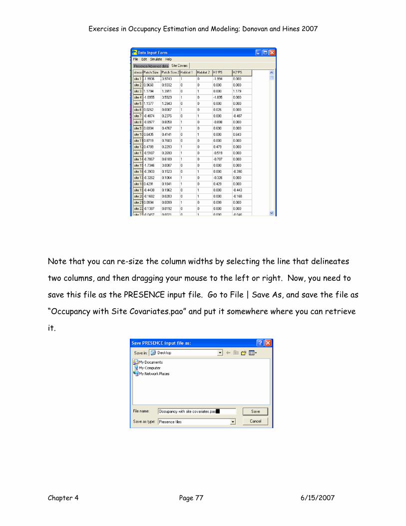
Exercises in Occupancy Estimation and Modeling; Donovan and Hines 2007
Chapter 4 Page 77 6/15/2007
Note that you can re-size the column widths by selecting the line that delineates
two columns, and then dragging your mouse to the left or right. Now, you need to
save this file as the PRESENCE input file. Go to File | Save As, and save the file as
“Occupancy with Site Covariates.pao” and put it somewhere where you can retrieve
it.
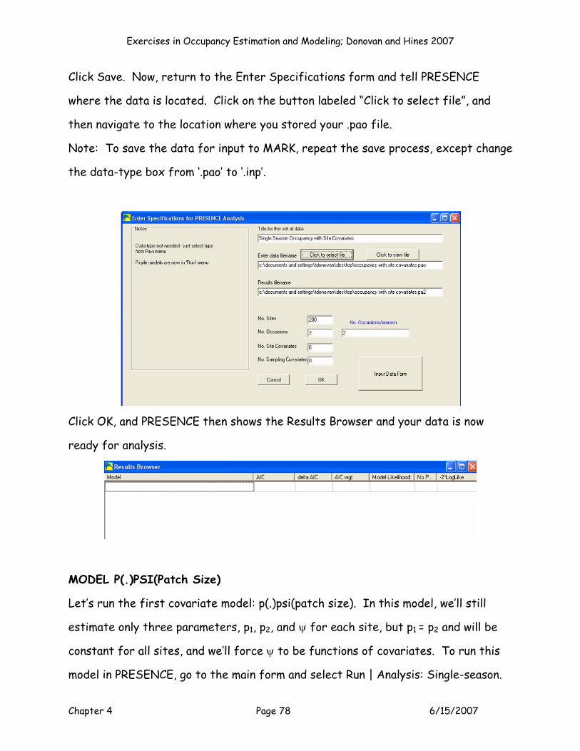
Exercises in Occupancy Estimation and Modeling; Donovan and Hines 2007
Chapter 4 Page 78 6/15/2007
Click Save. Now, return to the Enter Specifications form and tell PRESENCE
where the data is located. Click on the button labeled “Click to select file”, and
then navigate to the location where you stored your .pao file.
Note: To save the data for input to MARK, repeat the save process, except change
the data-type box from ‘.pao’ to ‘.inp’.
Click OK, and PRESENCE then shows the Results Browser and your data is now
ready for analysis.
MODEL P(.)PSI(Patch Size)
Let’s run the first covariate model: p(.)psi(patch size). In this model, we’ll still
estimate only three parameters, p1, p2, and ψ for each site, but p1 = p2 and will be
constant for all sites, and we’ll force ψ to be functions of covariates. To run this
model in PRESENCE, go to the main form and select Run | Analysis: Single-season.
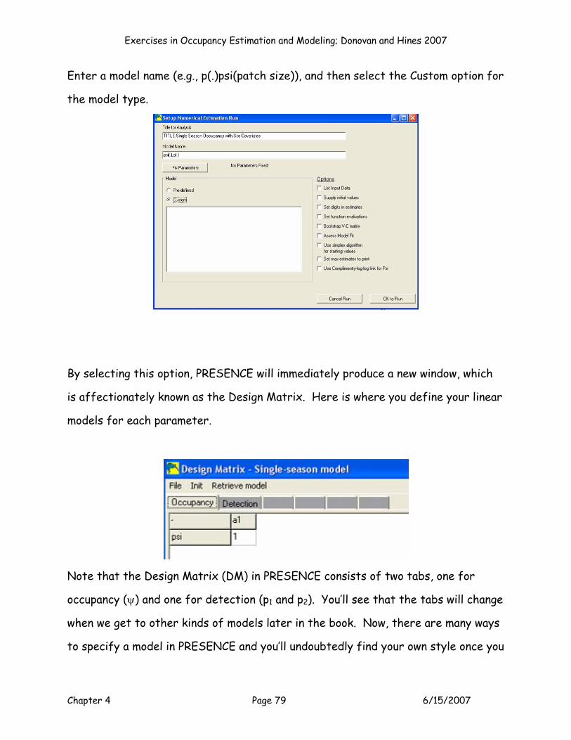
Exercises in Occupancy Estimation and Modeling; Donovan and Hines 2007
Chapter 4 Page 79 6/15/2007
Enter a model name (e.g., p(.)psi(patch size)), and then select the Custom option for
the model type.
By selecting this option, PRESENCE will immediately produce a new window, which
is affectionately known as the Design Matrix. Here is where you define your linear
models for each parameter.
Note that the Design Matrix (DM) in PRESENCE consists of two tabs, one for
occupancy (ψ) and one for detection (p1 and p2). You’ll see that the tabs will change
when we get to other kinds of models later in the book. Now, there are many ways
to specify a model in PRESENCE and you’ll undoubtedly find your own style once you
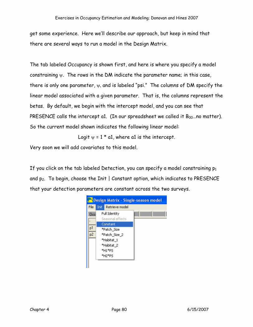
Exercises in Occupancy Estimation and Modeling; Donovan and Hines 2007
Chapter 4 Page 80 6/15/2007
get some experience. Here we’ll describe our approach, but keep in mind that
there are several ways to run a model in the Design Matrix.
The tab labeled Occupancy is shown first, and here is where you specify a model
constraining ψ. The rows in the DM indicate the parameter name; in this case,
there is only one parameter, ψ, and is labeled “psi.” The columns of DM specify the
linear model associated with a given parameter. That is, the columns represent the
betas. By default, we begin with the intercept model, and you can see that
PRESENCE calls the intercept a1. (In our spreadsheet we called it B00…no matter).
So the current model shown indicates the following linear model:
Logit ψ = 1 * a1, where a1 is the intercept.
Very soon we will add covariates to this model.
If you click on the tab labeled Detection, you can specify a model constraining p1
and p2. To begin, choose the Init | Constant option, which indicates to PRESENCE
that your detection parameters are constant across the two surveys.
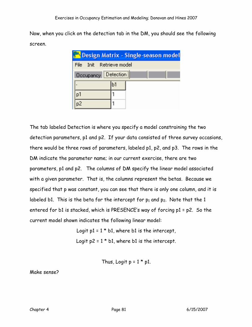
Exercises in Occupancy Estimation and Modeling; Donovan and Hines 2007
Chapter 4 Page 81 6/15/2007
Now, when you click on the detection tab in the DM, you should see the following
screen.
The tab labeled Detection is where you specify a model constraining the two
detection parameters, p1 and p2. If your data consisted of three survey occasions,
there would be three rows of parameters, labeled p1, p2, and p3. The rows in the
DM indicate the parameter name; in our current exercise, there are two
parameters, p1 and p2. The columns of DM specify the linear model associated
with a given parameter. That is, the columns represent the betas. Because we
specified that p was constant, you can see that there is only one column, and it is
labeled b1. This is the beta for the intercept for p1 and p2. Note that the 1
entered for b1 is stacked, which is PRESENCE’s way of forcing p1 = p2. So the
current model shown indicates the following linear model:
Logit p1 = 1 * b1, where b1 is the intercept,
Logit p2 = 1 * b1, where b1 is the intercept.
Thus, Logit p = 1 * p1.
Make sense?
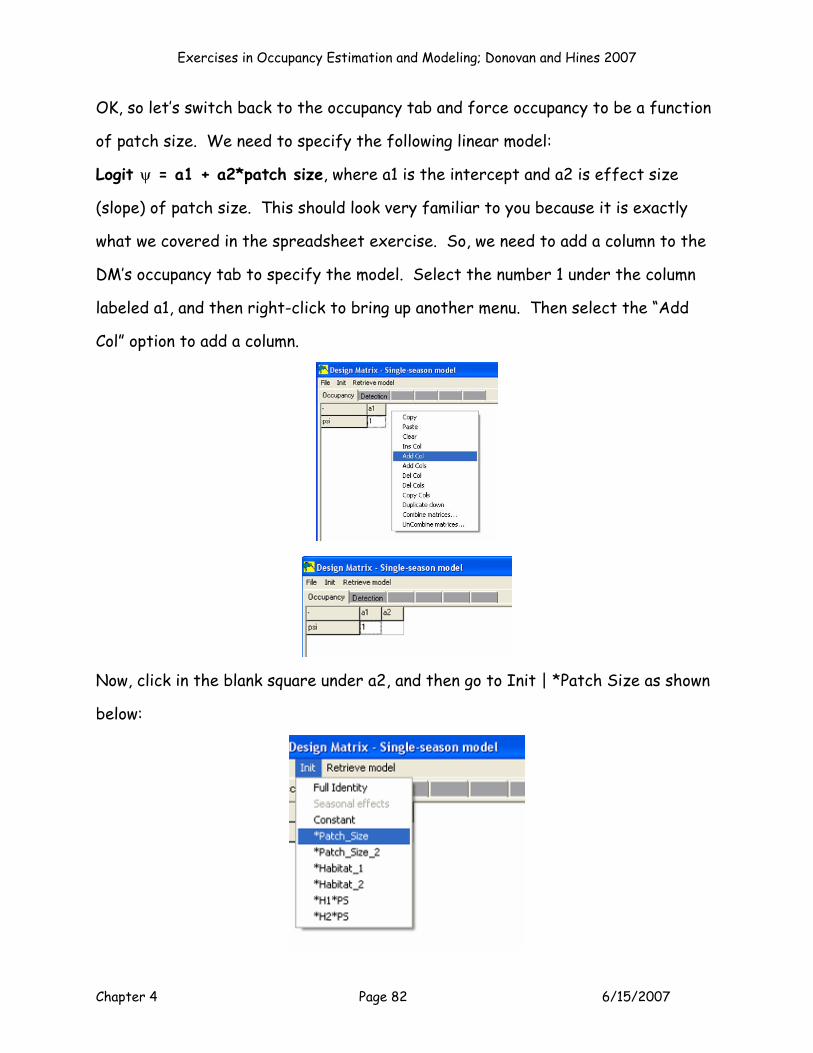
Exercises in Occupancy Estimation and Modeling; Donovan and Hines 2007
Chapter 4 Page 82 6/15/2007
OK, so let’s switch back to the occupancy tab and force occupancy to be a function
of patch size. We need to specify the following linear model:
Logit ψ = a1 + a2*patch size, where a1 is the intercept and a2 is effect size
(slope) of patch size. This should look very familiar to you because it is exactly
what we covered in the spreadsheet exercise. So, we need to add a column to the
DM’s occupancy tab to specify the model. Select the number 1 under the column
labeled a1, and then right-click to bring up another menu. Then select the “Add
Col” option to add a column.
Now, click in the blank square under a2, and then go to Init | *Patch Size as shown
below:
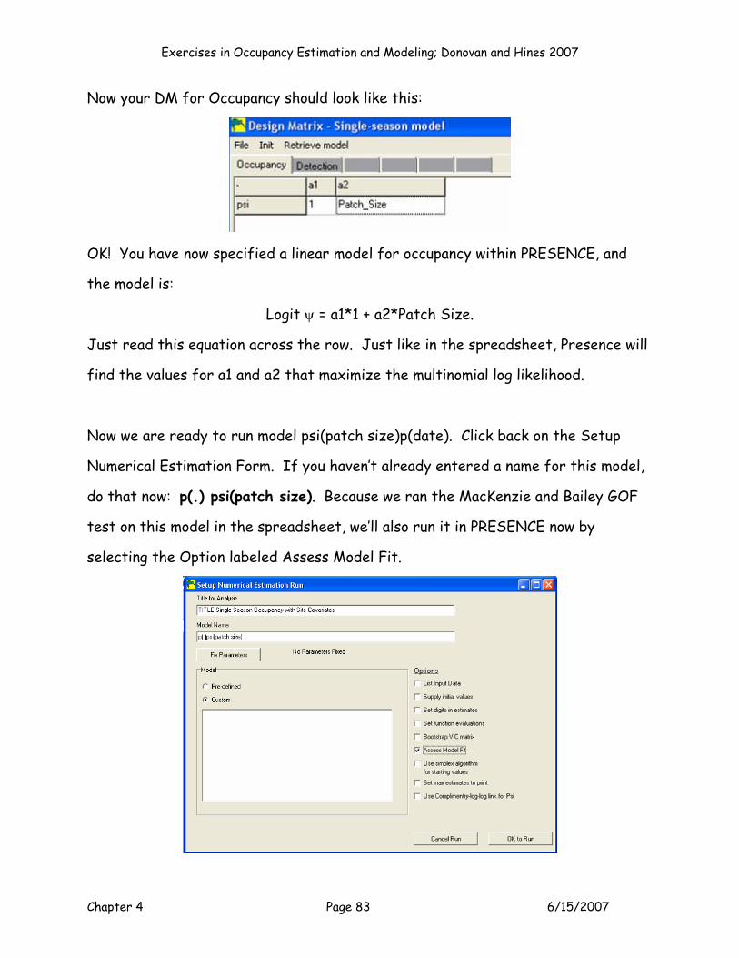
Exercises in Occupancy Estimation and Modeling; Donovan and Hines 2007
Chapter 4 Page 83 6/15/2007
Now your DM for Occupancy should look like this:
OK! You have now specified a linear model for occupancy within PRESENCE, and
the model is:
Logit ψ = a1*1 + a2*Patch Size.
Just read this equation across the row. Just like in the spreadsheet, Presence will
find the values for a1 and a2 that maximize the multinomial log likelihood.
Now we are ready to run model psi(patch size)p(date). Click back on the Setup
Numerical Estimation Form. If you haven’t already entered a name for this model,
do that now: p(.) psi(patch size). Because we ran the MacKenzie and Bailey GOF
test on this model in the spreadsheet, we’ll also run it in PRESENCE now by
selecting the Option labeled Assess Model Fit.
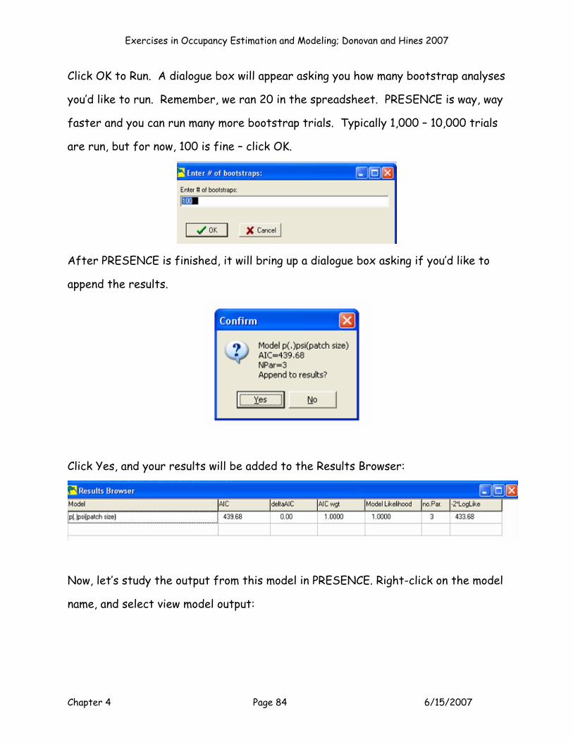
Exercises in Occupancy Estimation and Modeling; Donovan and Hines 2007
Chapter 4 Page 84 6/15/2007
Click OK to Run. A dialogue box will appear asking you how many bootstrap analyses
you’d like to run. Remember, we ran 20 in the spreadsheet. PRESENCE is way, way
faster and you can run many more bootstrap trials. Typically 1,000 – 10,000 trials
are run, but for now, 100 is fine – click OK.
After PRESENCE is finished, it will bring up a dialogue box asking if you’d like to
append the results.
Click Yes, and your results will be added to the Results Browser:
Now, let’s study the output from this model in PRESENCE. Right-click on the model
name, and select view model output:
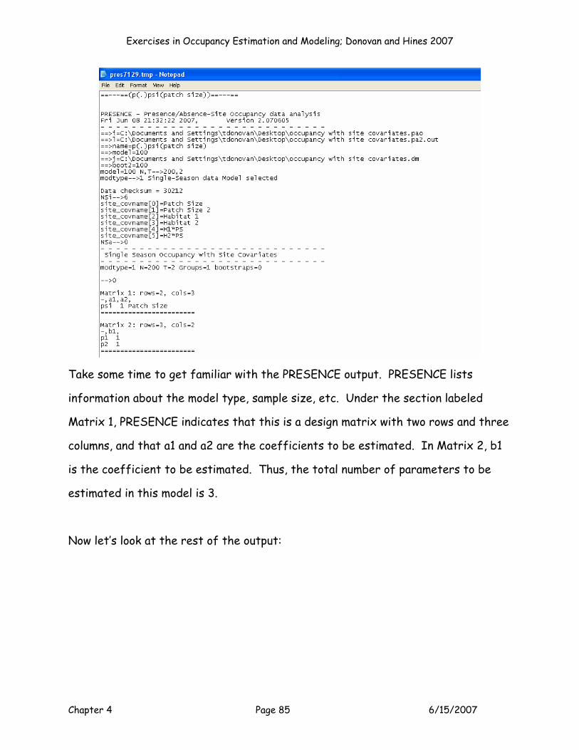
Exercises in Occupancy Estimation and Modeling; Donovan and Hines 2007
Chapter 4 Page 85 6/15/2007
Take some time to get familiar with the PRESENCE output. PRESENCE lists
information about the model type, sample size, etc. Under the section labeled
Matrix 1, PRESENCE indicates that this is a design matrix with two rows and three
columns, and that a1 and a2 are the coefficients to be estimated. In Matrix 2, b1
is the coefficient to be estimated. Thus, the total number of parameters to be
estimated in this model is 3.
Now let’s look at the rest of the output:
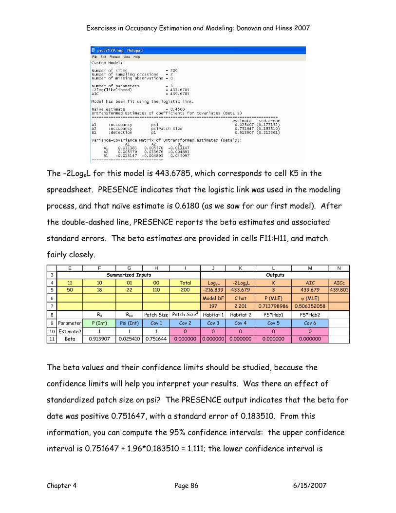
Exercises in Occupancy Estimation and Modeling; Donovan and Hines 2007
Chapter 4 Page 86 6/15/2007
The -2LogeL for this model is 443.6785, which corresponds to cell K5 in the
spreadsheet. PRESENCE indicates that the logistic link was used in the modeling
process, and that naïve estimate is 0.6180 (as we saw for our first model). After
the double-dashed line, PRESENCE reports the beta estimates and associated
standard errors. The beta estimates are provided in cells F11:H11, and match
fairly closely.
3
45
67
8
9
1011
E F G H I J K L M N
11 10 01 00 Total LogeL -2LogeL K AIC AICc50 18 22 110 200 -216.839 433.679 3 439.679 439.801
Model DF C hat P (MLE) ψ (MLE)197 2.201 0.713798986 0.506352058
B0 B00 Patch Size Patch Size2 Habitat 1 Habitat 2 PS*Hab1 PS*Hab2Parameter P (Int) Psi (Int) Cov 1 Cov 2 Cov 3 Cov 4 Cov 5 Cov 6Estimate? 1 1 1 0 0 0 0 0
Beta 0.913907 0.025410 0.751644 0.000000 0.000000 0.000000 0.000000 0.000000
Summarized Inputs Outputs
The beta values and their confidence limits should be studied, because the
confidence limits will help you interpret your results. Was there an effect of
standardized patch size on psi? The PRESENCE output indicates that the beta for
date was positive 0.751647, with a standard error of 0.183510. From this
information, you can compute the 95% confidence intervals: the upper confidence
interval is 0.751647 + 1.96*0.183510 = 1.111; the lower confidence interval is
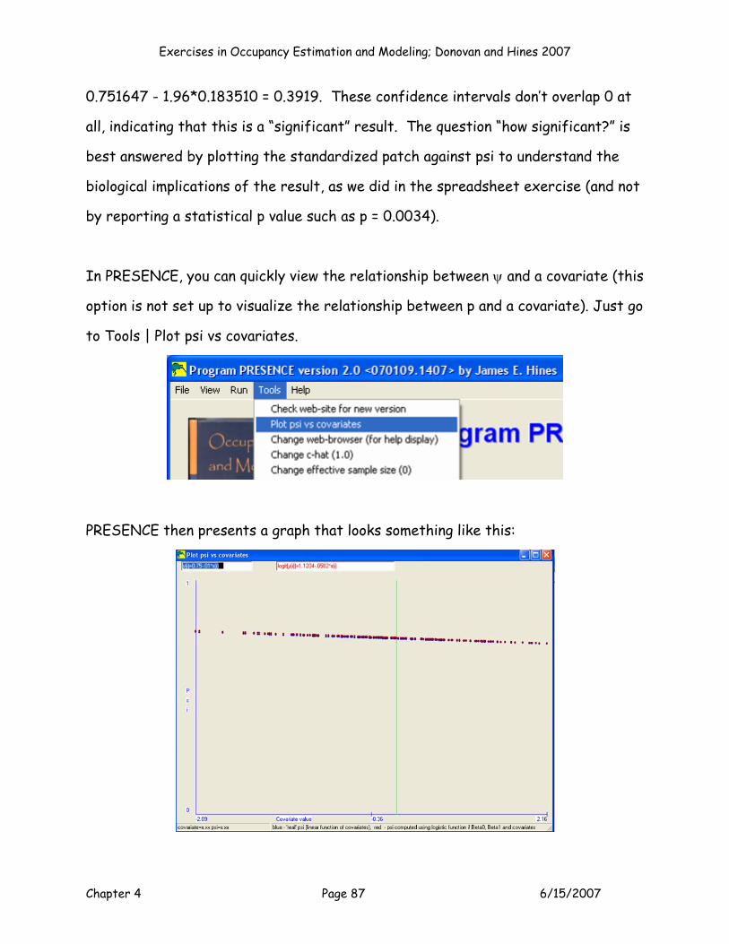
Exercises in Occupancy Estimation and Modeling; Donovan and Hines 2007
Chapter 4 Page 87 6/15/2007
0.751647 - 1.96*0.183510 = 0.3919. These confidence intervals don’t overlap 0 at
all, indicating that this is a “significant” result. The question “how significant?” is
best answered by plotting the standardized patch against psi to understand the
biological implications of the result, as we did in the spreadsheet exercise (and not
by reporting a statistical p value such as p = 0.0034).
In PRESENCE, you can quickly view the relationship between ψ and a covariate (this
option is not set up to visualize the relationship between p and a covariate). Just go
to Tools | Plot psi vs covariates.
PRESENCE then presents a graph that looks something like this:
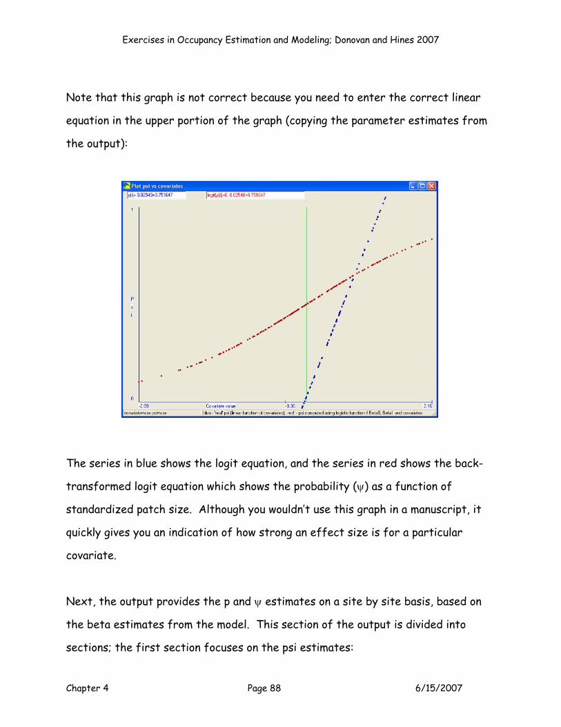
Exercises in Occupancy Estimation and Modeling; Donovan and Hines 2007
Chapter 4 Page 88 6/15/2007
Note that this graph is not correct because you need to enter the correct linear
equation in the upper portion of the graph (copying the parameter estimates from
the output):
The series in blue shows the logit equation, and the series in red shows the back-
transformed logit equation which shows the probability (ψ) as a function of
standardized patch size. Although you wouldn’t use this graph in a manuscript, it
quickly gives you an indication of how strong an effect size is for a particular
covariate.
Next, the output provides the p and ψ estimates on a site by site basis, based on
the beta estimates from the model. This section of the output is divided into
sections; the first section focuses on the psi estimates:
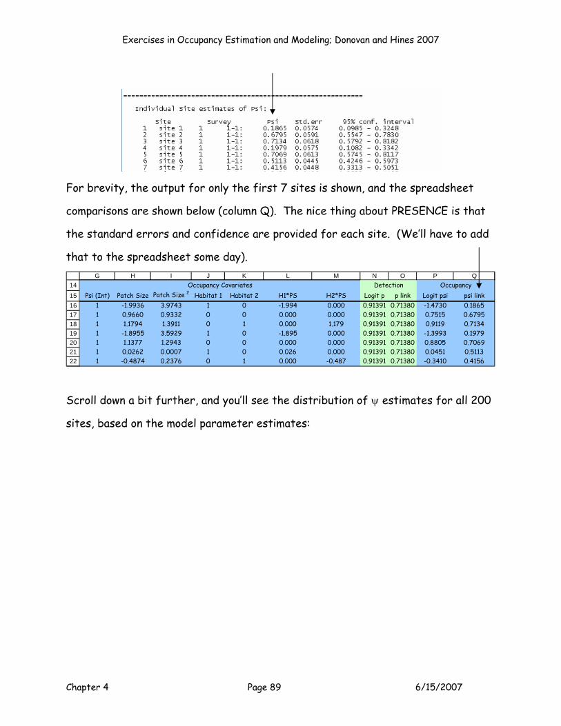
Exercises in Occupancy Estimation and Modeling; Donovan and Hines 2007
Chapter 4 Page 89 6/15/2007
For brevity, the output for only the first 7 sites is shown, and the spreadsheet
comparisons are shown below (column Q). The nice thing about PRESENCE is that
the standard errors and confidence are provided for each site. (We’ll have to add
that to the spreadsheet some day).
141516171819202122
G H I J K L M N O P Q
Psi (Int) Patch Size Patch Size 2 Habitat 1 Habitat 2 H1*PS H2*PS Logit p p link Logit psi psi link1 -1.9936 3.9743 1 0 -1.994 0.000 0.91391 0.71380 -1.4730 0.18651 0.9660 0.9332 0 0 0.000 0.000 0.91391 0.71380 0.7515 0.67951 1.1794 1.3911 0 1 0.000 1.179 0.91391 0.71380 0.9119 0.71341 -1.8955 3.5929 1 0 -1.895 0.000 0.91391 0.71380 -1.3993 0.19791 1.1377 1.2943 0 0 0.000 0.000 0.91391 0.71380 0.8805 0.70691 0.0262 0.0007 1 0 0.026 0.000 0.91391 0.71380 0.0451 0.51131 -0.4874 0.2376 0 1 0.000 -0.487 0.91391 0.71380 -0.3410 0.4156
Occupancy Covariates Detection Occupancy
Scroll down a bit further, and you’ll see the distribution of ψ estimates for all 200
sites, based on the model parameter estimates:
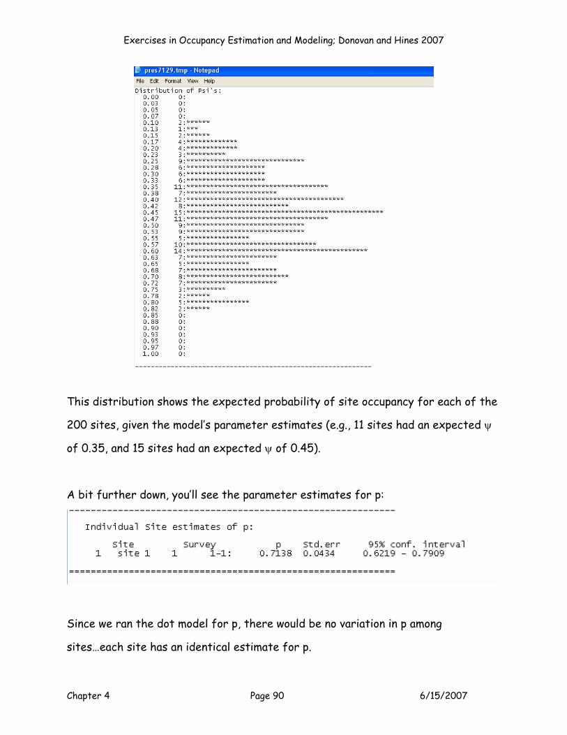
Exercises in Occupancy Estimation and Modeling; Donovan and Hines 2007
Chapter 4 Page 90 6/15/2007
This distribution shows the expected probability of site occupancy for each of the
200 sites, given the model’s parameter estimates (e.g., 11 sites had an expected ψ
of 0.35, and 15 sites had an expected ψ of 0.45).
A bit further down, you’ll see the parameter estimates for p:
Since we ran the dot model for p, there would be no variation in p among
sites…each site has an identical estimate for p.
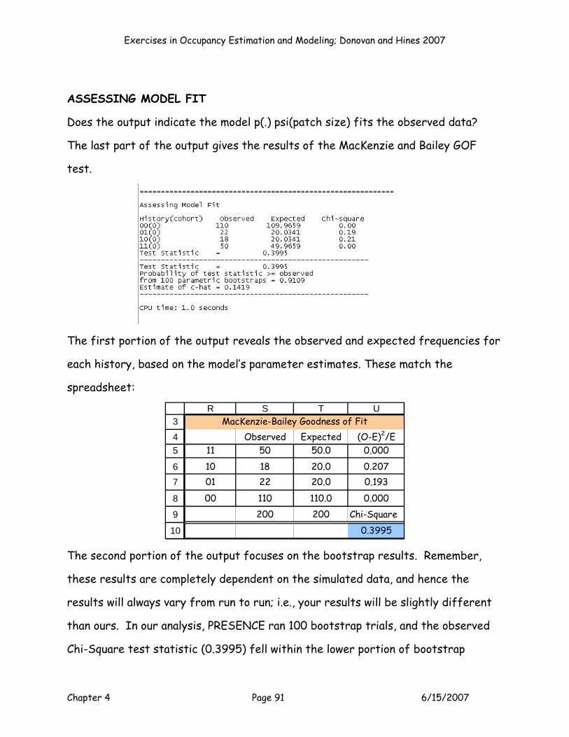
Exercises in Occupancy Estimation and Modeling; Donovan and Hines 2007
Chapter 4 Page 91 6/15/2007
ASSESSING MODEL FIT
Does the output indicate the model p(.) psi(patch size) fits the observed data?
The last part of the output gives the results of the MacKenzie and Bailey GOF
test.
The first portion of the output reveals the observed and expected frequencies for
each history, based on the model’s parameter estimates. These match the
spreadsheet:
3
45
67
8
9
10
R S T U
Observed Expected (O-E)2/E11 50 50.0 0.00010 18 20.0 0.20701 22 20.0 0.193
00 110 110.0 0.000200 200 Chi-Square
0.3995
MacKenzie-Bailey Goodness of Fit
The second portion of the output focuses on the bootstrap results. Remember,
these results are completely dependent on the simulated data, and hence the
results will always vary from run to run; i.e., your results will be slightly different
than ours. In our analysis, PRESENCE ran 100 bootstrap trials, and the observed
Chi-Square test statistic (0.3995) fell within the lower portion of bootstrap
Exercises in Occupancy Estimation and Modeling; Donovan and Hines 2007
Chapter 4 Page 92 6/15/2007
distribution. Specifically, 91.09% of the bootstrap Chi-Square values were larger
than 0.399, and (1-91.09%) = 8.91% of the bootstrap Chi-Square values were
smaller than the observed value. Based on these results, we can conclude that
there is no evidence of lack-of-fit. These results are not very consistent in the
100 spreadsheet runs (I’m not sure why), where the observed test statistic is given
in cells AN8, and the percentile is given in cell AN9.
8
9
1011
AM ANChi-SquareR 0.399469401Percentile 0.49
Chi-SquareB 1.343354815c hat 0.297367008
Now, you have a choice of what to do next. First, because the observed data
appear to “fit” the model, you can continue running models with a clear conscience.
If c-hat was greater than 1, you want to adjust c-hat because many analysts feel
that any c-hat estimate greater than 1 potentially biases the standard error
estimates. To do this, return to the main menu and go to Tools | Change c-hat.
Then enter the new c-hat value, and click OK. You should see that the standard
errors for the different parameter estimates have increased as a result.
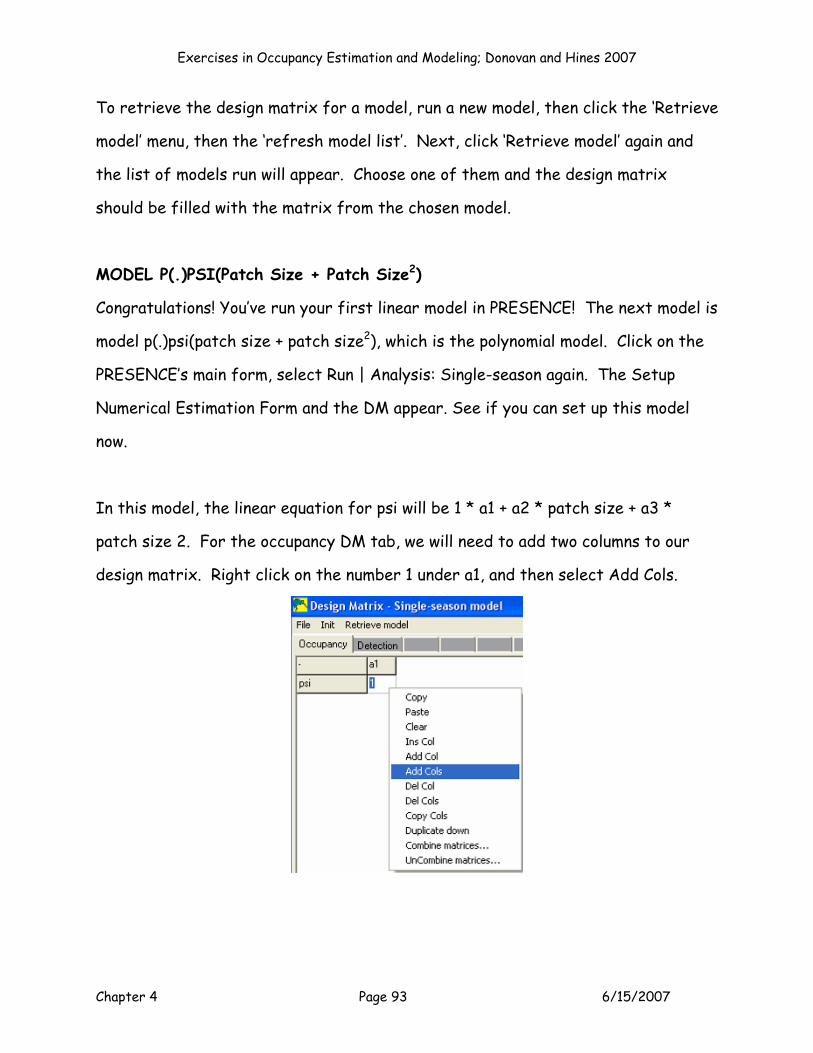
Exercises in Occupancy Estimation and Modeling; Donovan and Hines 2007
Chapter 4 Page 93 6/15/2007
To retrieve the design matrix for a model, run a new model, then click the ‘Retrieve
model’ menu, then the ‘refresh model list’. Next, click ‘Retrieve model’ again and
the list of models run will appear. Choose one of them and the design matrix
should be filled with the matrix from the chosen model.
MODEL P(.)PSI(Patch Size + Patch Size2)
Congratulations! You’ve run your first linear model in PRESENCE! The next model is
model p(.)psi(patch size + patch size2), which is the polynomial model. Click on the
PRESENCE’s main form, select Run | Analysis: Single-season again. The Setup
Numerical Estimation Form and the DM appear. See if you can set up this model
now.
In this model, the linear equation for psi will be 1 * a1 + a2 * patch size + a3 *
patch size 2. For the occupancy DM tab, we will need to add two columns to our
design matrix. Right click on the number 1 under a1, and then select Add Cols.
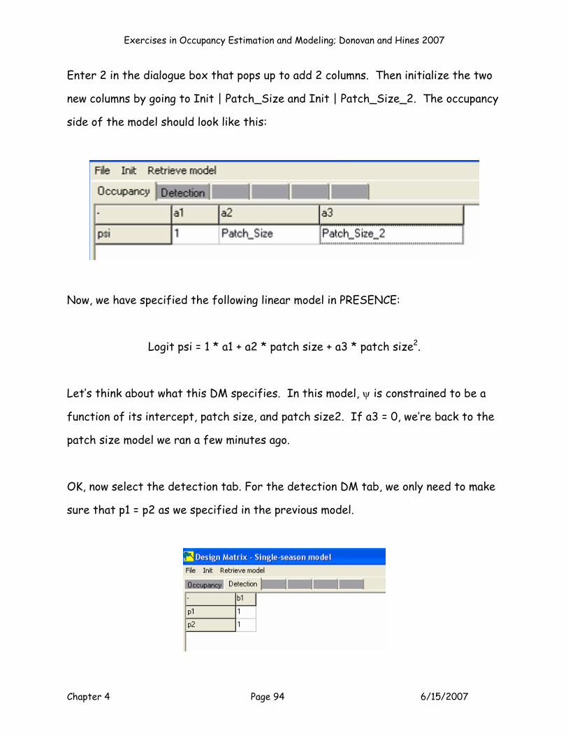
Exercises in Occupancy Estimation and Modeling; Donovan and Hines 2007
Chapter 4 Page 94 6/15/2007
Enter 2 in the dialogue box that pops up to add 2 columns. Then initialize the two
new columns by going to Init | Patch_Size and Init | Patch_Size_2. The occupancy
side of the model should look like this:
Now, we have specified the following linear model in PRESENCE:
Logit psi = 1 * a1 + a2 * patch size + a3 * patch size2.
Let’s think about what this DM specifies. In this model, ψ is constrained to be a
function of its intercept, patch size, and patch size2. If a3 = 0, we’re back to the
patch size model we ran a few minutes ago.
OK, now select the detection tab. For the detection DM tab, we only need to make
sure that p1 = p2 as we specified in the previous model.
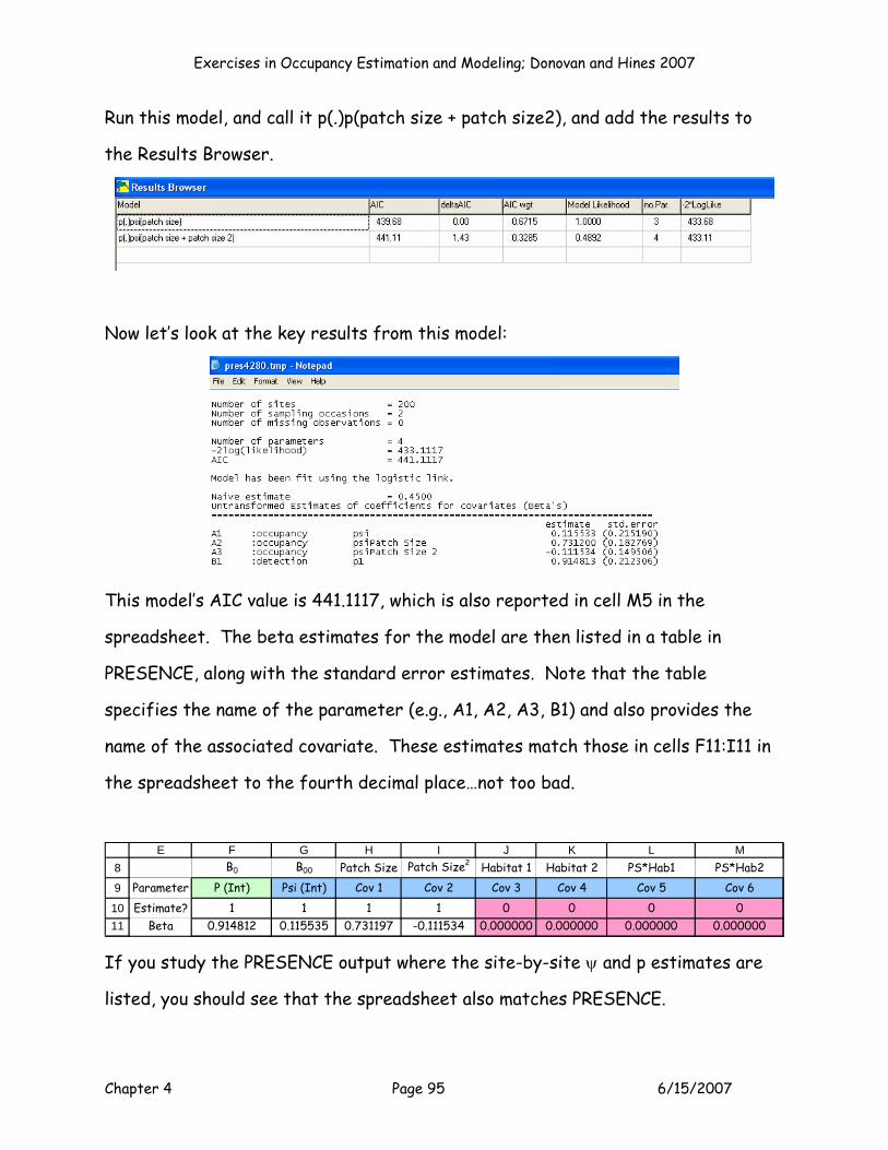
Exercises in Occupancy Estimation and Modeling; Donovan and Hines 2007
Chapter 4 Page 95 6/15/2007
Run this model, and call it p(.)p(patch size + patch size2), and add the results to
the Results Browser.
Now let’s look at the key results from this model:
This model’s AIC value is 441.1117, which is also reported in cell M5 in the
spreadsheet. The beta estimates for the model are then listed in a table in
PRESENCE, along with the standard error estimates. Note that the table
specifies the name of the parameter (e.g., A1, A2, A3, B1) and also provides the
name of the associated covariate. These estimates match those in cells F11:I11 in
the spreadsheet to the fourth decimal place…not too bad.
8
9
1011
E F G H I J K L MB0 B00 Patch Size Patch Size2 Habitat 1 Habitat 2 PS*Hab1 PS*Hab2
Parameter P (Int) Psi (Int) Cov 1 Cov 2 Cov 3 Cov 4 Cov 5 Cov 6Estimate? 1 1 1 1 0 0 0 0
Beta 0.914812 0.115535 0.731197 -0.111534 0.000000 0.000000 0.000000 0.000000
If you study the PRESENCE output where the site-by-site ψ and p estimates are
listed, you should see that the spreadsheet also matches PRESENCE.
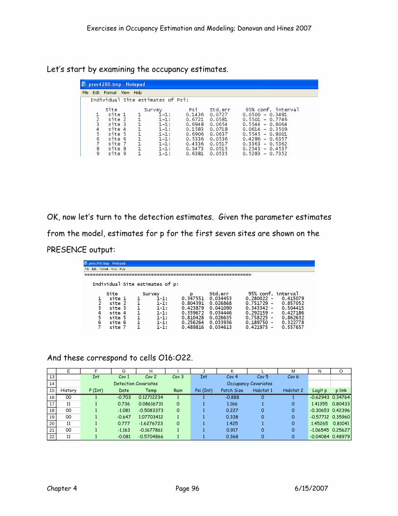
Exercises in Occupancy Estimation and Modeling; Donovan and Hines 2007
Chapter 4 Page 96 6/15/2007
Let’s start by examining the occupancy estimates.
OK, now let’s turn to the detection estimates. Given the parameter estimates
from the model, estimates for p for the first seven sites are shown on the
PRESENCE output:
And these correspond to cells O16:O22.
13141516171819202122
E F G H I J K L M N OInt Cov 1 Cov 2 Cov 3 Int Cov 4 Cov 5 Cov 6
History P (Int) Date Temp Rain Psi (Int) Patch Size Habitat 1 Habitat 2 Logit p p link00 1 -0.703 0.12712234 1 1 -0.888 0 1 -0.62943 0.3476411 1 0.736 0.08616731 0 1 1.166 1 0 1.41355 0.8043300 1 -1.081 -0.5083373 0 1 0.227 0 0 -0.30653 0.4239600 1 -0.647 1.07703412 1 1 0.338 0 0 -0.57712 0.3596011 1 0.777 -1.6276723 0 1 1.425 1 0 1.45265 0.8104100 1 -1.163 -0.1677861 1 1 0.917 0 0 -1.06545 0.2562711 1 -0.081 -0.5704866 1 1 0.368 0 0 -0.04084 0.48979
Detection Covariates Occupancy Covariates
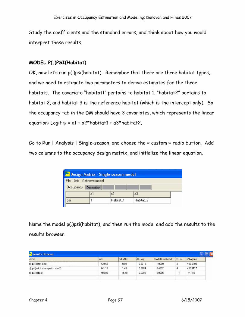
Exercises in Occupancy Estimation and Modeling; Donovan and Hines 2007
Chapter 4 Page 97 6/15/2007
Study the coefficients and the standard errors, and think about how you would
interpret these results.
MODEL P(.)PSI(Habitat)
OK, now let’s run p(.)psi(habitat). Remember that there are three habitat types,
and we need to estimate two parameters to derive estimates for the three
habitats. The covariate “habitat1” pertains to habitat 1, “habitat2” pertains to
habitat 2, and habitat 3 is the reference habitat (which is the intercept only). So
the occupancy tab in the DM should have 3 covariates, which represents the linear
equation: Logit ψ = a1 + a2*habitat1 + a3*habitat2.
Go to Run | Analysis | Single-season, and choose the « custom » radio button. Add
two columns to the occupancy design matrix, and initialize the linear equation.
Name the model p(.)psi(habitat), and then run the model and add the results to the
results browser.
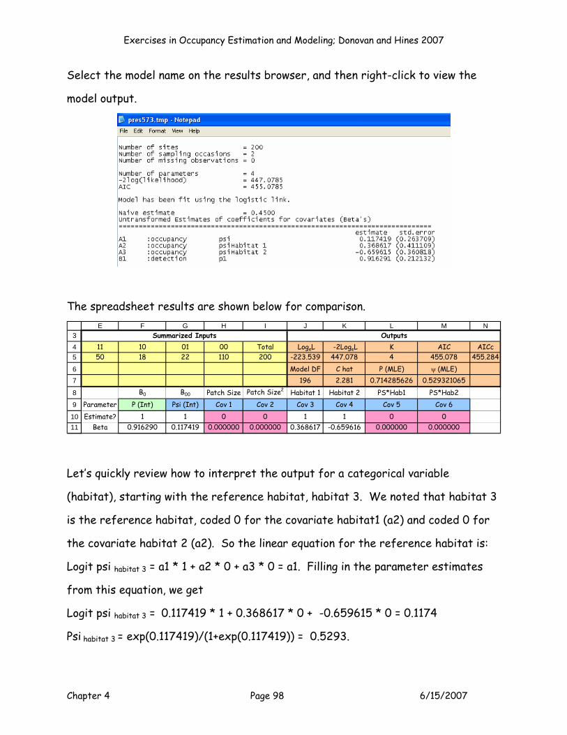
Exercises in Occupancy Estimation and Modeling; Donovan and Hines 2007
Chapter 4 Page 98 6/15/2007
Select the model name on the results browser, and then right-click to view the
model output.
The spreadsheet results are shown below for comparison.
3
45
67
8
9
1011
E F G H I J K L M N
11 10 01 00 Total LogeL -2LogeL K AIC AICc50 18 22 110 200 -223.539 447.078 4 455.078 455.284
Model DF C hat P (MLE) ψ (MLE)196 2.281 0.714285626 0.529321065
B0 B00 Patch Size Patch Size2 Habitat 1 Habitat 2 PS*Hab1 PS*Hab2Parameter P (Int) Psi (Int) Cov 1 Cov 2 Cov 3 Cov 4 Cov 5 Cov 6Estimate? 1 1 0 0 1 1 0 0
Beta 0.916290 0.117419 0.000000 0.000000 0.368617 -0.659616 0.000000 0.000000
Summarized Inputs Outputs
Let’s quickly review how to interpret the output for a categorical variable
(habitat), starting with the reference habitat, habitat 3. We noted that habitat 3
is the reference habitat, coded 0 for the covariate habitat1 (a2) and coded 0 for
the covariate habitat 2 (a2). So the linear equation for the reference habitat is:
Logit psi habitat 3 = a1 * 1 + a2 * 0 + a3 * 0 = a1. Filling in the parameter estimates
from this equation, we get
Logit psi habitat 3 = 0.117419 * 1 + 0.368617 * 0 + -0.659615 * 0 = 0.1174
Psi habitat 3 = exp(0.117419)/(1+exp(0.117419)) = 0.5293.
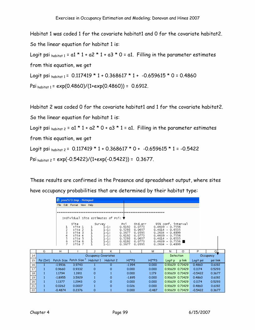
Exercises in Occupancy Estimation and Modeling; Donovan and Hines 2007
Chapter 4 Page 99 6/15/2007
Habitat 1 was coded 1 for the covariate habitat1 and 0 for the covariate habitat2.
So the linear equation for habitat 1 is:
Logit psi habitat 1 = a1 * 1 + a2 * 1 + a3 * 0 = a1. Filling in the parameter estimates
from this equation, we get
Logit psi habitat 1 = 0.117419 * 1 + 0.368617 * 1 + -0.659615 * 0 = 0.4860
Psi habitat 1 = exp(0.4860)/(1+exp(0.4860)) = 0.6912.
Habitat 2 was coded 0 for the covariate habitat1 and 1 for the covariate habitat2.
So the linear equation for habitat 1 is:
Logit psi habitat 2 = a1 * 1 + a2 * 0 + a3 * 1 = a1. Filling in the parameter estimates
from this equation, we get
Logit psi habitat 2 = 0.117419 * 1 + 0.368617 * 0 + -0.659615 * 1 = -0.5422
Psi habitat 2 = exp(-0.5422)/(1+exp(-0.5422)) = 0.3677.
These results are confirmed in the Presence and spreadsheet output, where sites
have occupancy probabilities that are determined by their habitat type:
141516171819202122
G H I J K L M N O P Q
Psi (Int) Patch Size Patch Size 2 Habitat 1 Habitat 2 H1*PS H2*PS Logit p p link Logit psi psi link1 -1.9936 3.9743 1 0 -1.994 0.000 0.91629 0.71429 0.4860 0.61921 0.9660 0.9332 0 0 0.000 0.000 0.91629 0.71429 0.1174 0.52931 1.1794 1.3911 0 1 0.000 1.179 0.91629 0.71429 -0.5422 0.36771 -1.8955 3.5929 1 0 -1.895 0.000 0.91629 0.71429 0.4860 0.61921 1.1377 1.2943 0 0 0.000 0.000 0.91629 0.71429 0.1174 0.52931 0.0262 0.0007 1 0 0.026 0.000 0.91629 0.71429 0.4860 0.61921 -0.4874 0.2376 0 1 0.000 -0.487 0.91629 0.71429 -0.5422 0.3677
Occupancy Covariates Detection Occupancy
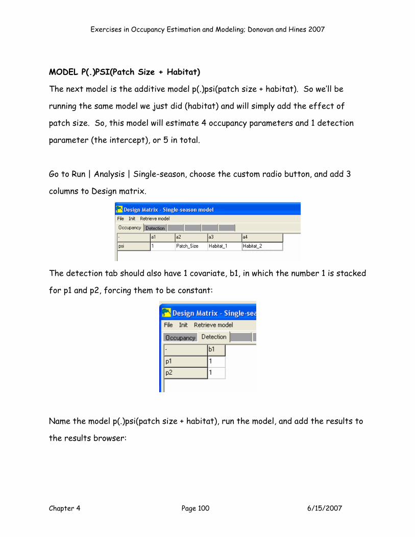
Exercises in Occupancy Estimation and Modeling; Donovan and Hines 2007
Chapter 4 Page 100 6/15/2007
MODEL P(.)PSI(Patch Size + Habitat)
The next model is the additive model p(.)psi(patch size + habitat). So we’ll be
running the same model we just did (habitat) and will simply add the effect of
patch size. So, this model will estimate 4 occupancy parameters and 1 detection
parameter (the intercept), or 5 in total.
Go to Run | Analysis | Single-season, choose the custom radio button, and add 3
columns to Design matrix.
The detection tab should also have 1 covariate, b1, in which the number 1 is stacked
for p1 and p2, forcing them to be constant:
Name the model p(.)psi(patch size + habitat), run the model, and add the results to
the results browser:
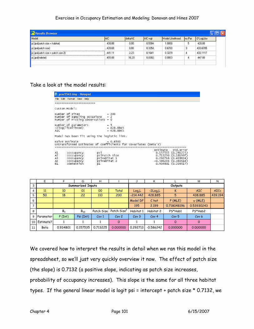
Exercises in Occupancy Estimation and Modeling; Donovan and Hines 2007
Chapter 4 Page 101 6/15/2007
Take a look at the model results:
3
45
67
8
9
10
11
E F G H I J K L M N
11 10 01 00 Total LogeL -2LogeL K AIC AICc50 18 22 110 200 -214.442 428.885 5 438.885 439.194
Model DF C hat P (MLE) ψ (MLE)195 2.199 0.718048196 0.53930243
B0 B00 Patch Size Patch Size2 Habitat 1 Habitat 2 PS*Hab1 PS*Hab2Parameter P (Int) Psi (Int) Cov 1 Cov 2 Cov 3 Cov 4 Cov 5 Cov 6Estimate? 1 1 1 0 1 1 0 0
Beta 0.934801 0.157535 0.713225 0.000000 0.292713 -0.586242 0.000000 0.000000
Summarized Inputs Outputs
We covered how to interpret the results in detail when we ran this model in the
spreadsheet, so we’ll just very quickly overview it now. The effect of patch size
(the slope) is 0.7132 (a positive slope, indicating as patch size increases,
probability of occupancy increases). This slope is the same for all three habitat
types. If the general linear model is logit psi = intercept + patch size * 0.7132, we
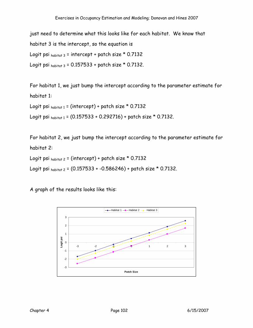
Exercises in Occupancy Estimation and Modeling; Donovan and Hines 2007
Chapter 4 Page 102 6/15/2007
just need to determine what this looks like for each habitat. We know that
habitat 3 is the intercept, so the equation is
Logit psi habitat 3 = intercept + patch size * 0.7132
Logit psi habitat 3 = 0.157533 + patch size * 0.7132.
For habitat 1, we just bump the intercept according to the parameter estimate for
habitat 1:
Logit psi habitat 1 = (intercept) + patch size * 0.7132
Logit psi habitat 1 = (0.157533 + 0.292716) + patch size * 0.7132.
For habitat 2, we just bump the intercept according to the parameter estimate for
habitat 2:
Logit psi habitat 2 = (intercept) + patch size * 0.7132
Logit psi habitat 2 = (0.157533 + -0.586246) + patch size * 0.7132.
A graph of the results looks like this:
-3
-2
-1
0
1
2
3
-3 -2 -1 0 1 2 3
Patch Size
Logi
t psi
Habitat 1 Habitat 2 Habitat 3
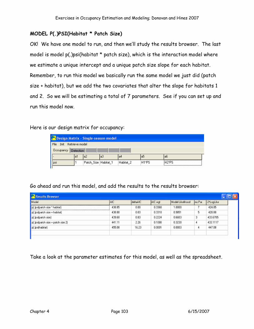
Exercises in Occupancy Estimation and Modeling; Donovan and Hines 2007
Chapter 4 Page 103 6/15/2007
MODEL P(.)PSI(Habitat * Patch Size)
OK! We have one model to run, and then we’ll study the results browser. The last
model is model p(.)psi(habitat * patch size), which is the interaction model where
we estimate a unique intercept and a unique patch size slope for each habitat.
Remember, to run this model we basically run the same model we just did (patch
size + habitat), but we add the two covariates that alter the slope for habitats 1
and 2. So we will be estimating a total of 7 parameters. See if you can set up and
run this model now.
Here is our design matrix for occupancy:
Go ahead and run this model, and add the results to the results browser:
Take a look at the parameter estimates for this model, as well as the spreadsheet.
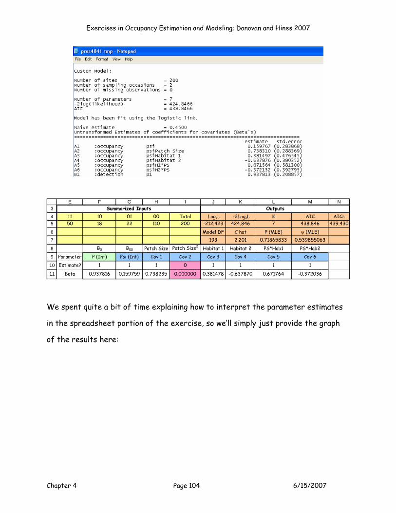
Exercises in Occupancy Estimation and Modeling; Donovan and Hines 2007
Chapter 4 Page 104 6/15/2007
3
45
67
8
9
10
11
E F G H I J K L M N
11 10 01 00 Total LogeL -2LogeL K AIC AICc50 18 22 110 200 -212.423 424.846 7 438.846 439.430
Model DF C hat P (MLE) ψ (MLE)193 2.201 0.71865833 0.539855063
B0 B00 Patch Size Patch Size2 Habitat 1 Habitat 2 PS*Hab1 PS*Hab2Parameter P (Int) Psi (Int) Cov 1 Cov 2 Cov 3 Cov 4 Cov 5 Cov 6Estimate? 1 1 1 0 1 1 1 1
Beta 0.937816 0.159759 0.738235 0.000000 0.381478 -0.637870 0.671764 -0.372036
Summarized Inputs Outputs
We spent quite a bit of time explaining how to interpret the parameter estimates
in the spreadsheet portion of the exercise, so we’ll simply just provide the graph
of the results here:
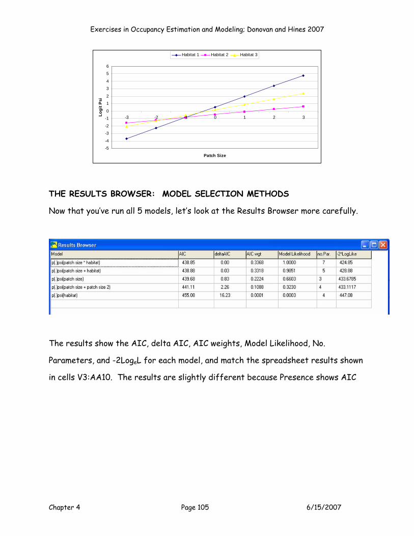
Exercises in Occupancy Estimation and Modeling; Donovan and Hines 2007
Chapter 4 Page 105 6/15/2007
-5
-4
-3
-2
-1
0
1
2
3
4
5
6
-3 -2 -1 0 1 2 3
Patch Size
Logi
t Psi
Habitat 1 Habitat 2 Habitat 3
THE RESULTS BROWSER: MODEL SELECTION METHODS
Now that you’ve run all 5 models, let’s look at the Results Browser more carefully.
The results show the AIC, delta AIC, AIC weights, Model Likelihood, No.
Parameters, and -2LogeL for each model, and match the spreadsheet results shown
in cells V3:AA10. The results are slightly different because Presence shows AIC
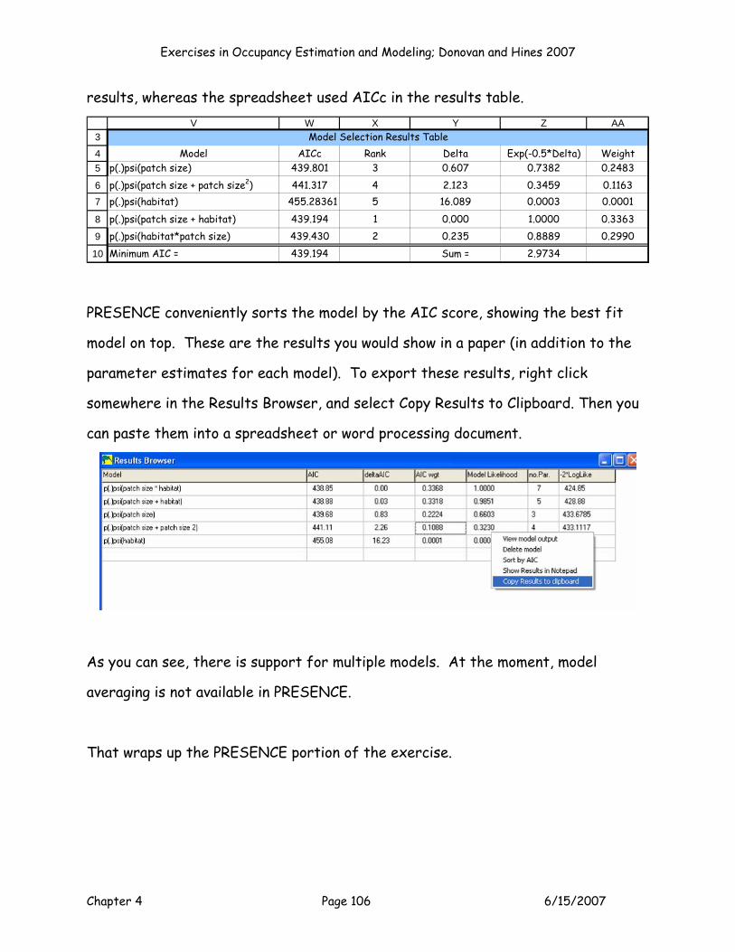
Exercises in Occupancy Estimation and Modeling; Donovan and Hines 2007
Chapter 4 Page 106 6/15/2007
results, whereas the spreadsheet used AICc in the results table.
3
45
67
8
9
10
V W X Y Z AA
Model AICc Rank Delta Exp(-0.5*Delta) Weightp(.)psi(patch size) 439.801 3 0.607 0.7382 0.2483p(.)psi(patch size + patch size2) 441.317 4 2.123 0.3459 0.1163p(.)psi(habitat) 455.28361 5 16.089 0.0003 0.0001
p(.)psi(patch size + habitat) 439.194 1 0.000 1.0000 0.3363p(.)psi(habitat*patch size) 439.430 2 0.235 0.8889 0.2990Minimum AIC = 439.194 Sum = 2.9734
Model Selection Results Table
PRESENCE conveniently sorts the model by the AIC score, showing the best fit
model on top. These are the results you would show in a paper (in addition to the
parameter estimates for each model). To export these results, right click
somewhere in the Results Browser, and select Copy Results to Clipboard. Then you
can paste them into a spreadsheet or word processing document.
As you can see, there is support for multiple models. At the moment, model
averaging is not available in PRESENCE.
That wraps up the PRESENCE portion of the exercise.
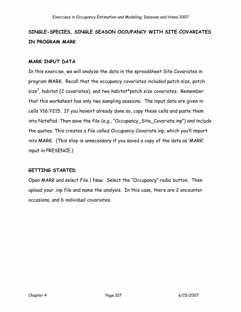
Exercises in Occupancy Estimation and Modeling; Donovan and Hines 2007
Chapter 4 Page 107 6/15/2007
SINGLE-SPECIES, SINGLE SEASON OCCUPANCY WITH SITE COVARIATES
IN PROGRAM MARK
MARK INPUT DATA
In this exercise, we will analyze the data in the spreadsheet Site Covariates in
program MARK. Recall that the occupancy covariates included patch size, patch
size2, habitat (2 covariates), and two habitat*patch size covariates. Remember
that this worksheet has only two sampling sessions. The input data are given in
cells Y16:Y215. If you haven’t already done so, copy these cells and paste them
into NotePad. Then save the file (e.g., “Occupancy_Site_Covariate.inp”) and include
the quotes. This creates a file called Occupancy Covariate.inp, which you’ll import
into MARK. (This step is unnecessary if you saved a copy of the data as ‘MARK’
input in PRESENCE.)
GETTING STARTED
Open MARK and select File | New. Select the “Occupancy” radio button. Then
upload your .inp file and name the analysis. In this case, there are 2 encounter
occasions, and 6 individual covariates.
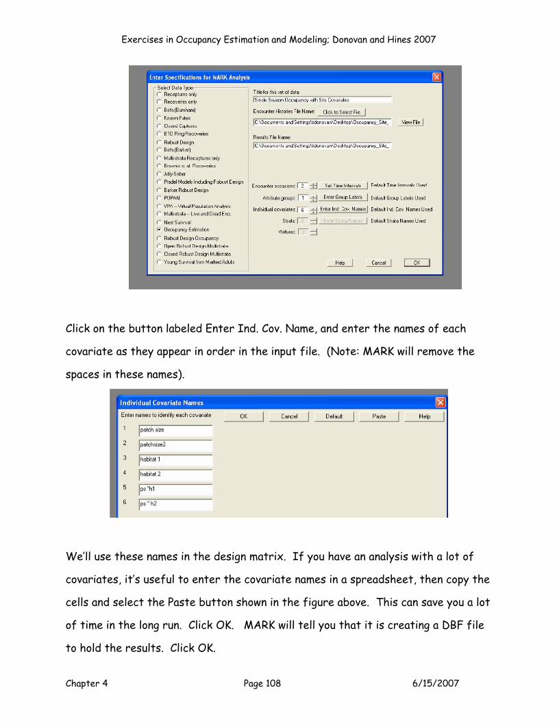
Exercises in Occupancy Estimation and Modeling; Donovan and Hines 2007
Chapter 4 Page 108 6/15/2007
Click on the button labeled Enter Ind. Cov. Name, and enter the names of each
covariate as they appear in order in the input file. (Note: MARK will remove the
spaces in these names).
We’ll use these names in the design matrix. If you have an analysis with a lot of
covariates, it’s useful to enter the covariate names in a spreadsheet, then copy the
cells and select the Paste button shown in the figure above. This can save you a lot
of time in the long run. Click OK. MARK will tell you that it is creating a DBF file
to hold the results. Click OK.
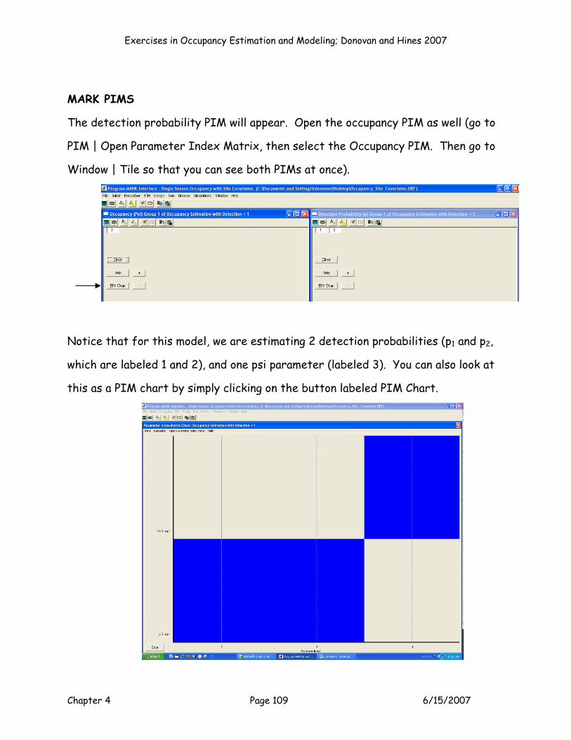
Exercises in Occupancy Estimation and Modeling; Donovan and Hines 2007
Chapter 4 Page 109 6/15/2007
MARK PIMS
The detection probability PIM will appear. Open the occupancy PIM as well (go to
PIM | Open Parameter Index Matrix, then select the Occupancy PIM. Then go to
Window | Tile so that you can see both PIMs at once).
Notice that for this model, we are estimating 2 detection probabilities (p1 and p2,
which are labeled 1 and 2), and one psi parameter (labeled 3). You can also look at
this as a PIM chart by simply clicking on the button labeled PIM Chart.
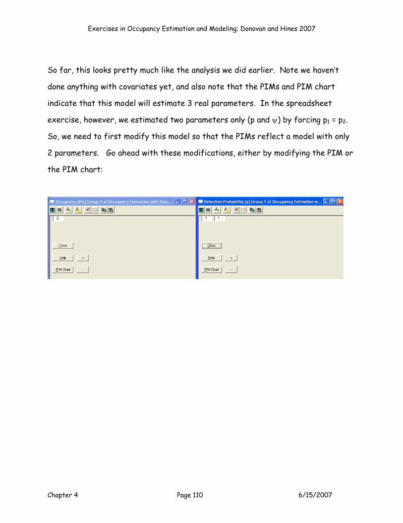
Exercises in Occupancy Estimation and Modeling; Donovan and Hines 2007
Chapter 4 Page 110 6/15/2007
So far, this looks pretty much like the analysis we did earlier. Note we haven’t
done anything with covariates yet, and also note that the PIMs and PIM chart
indicate that this model will estimate 3 real parameters. In the spreadsheet
exercise, however, we estimated two parameters only (p and ψ) by forcing p1 = p2.
So, we need to first modify this model so that the PIMs reflect a model with only
2 parameters. Go ahead with these modifications, either by modifying the PIM or
the PIM chart:

Exercises in Occupancy Estimation and Modeling; Donovan and Hines 2007
Chapter 4 Page 111 6/15/2007
If we were to run this model right now, it would be called p(.)psi(.). Parameter 1 is
the estimate the intercept for p, and parameter 2 is the estimate for the
intercept for psi. But since this isn’t part of our model set, we won’t run it.
However, it will be the basis for the models that we’ll run.
MODEL P(.)PSI(Patch Size)
The first model is model p(.)psi(patch size), where we’ll force psi to be a function
of patch size. Remember, we model linear equations (logits), and then will back-
transform the logits to probabilities (ψ and p) with the logit link. We’ll use the
Design Matrix to constrain occupancy to be a function of the covariate patch size.
Now, there are several ways to develop a Design Matrix…..we’ll describe one
approach, but you’ll undoubtedly form your own preferences as you become familiar
with MARK, and will pick up some short cuts along the way.
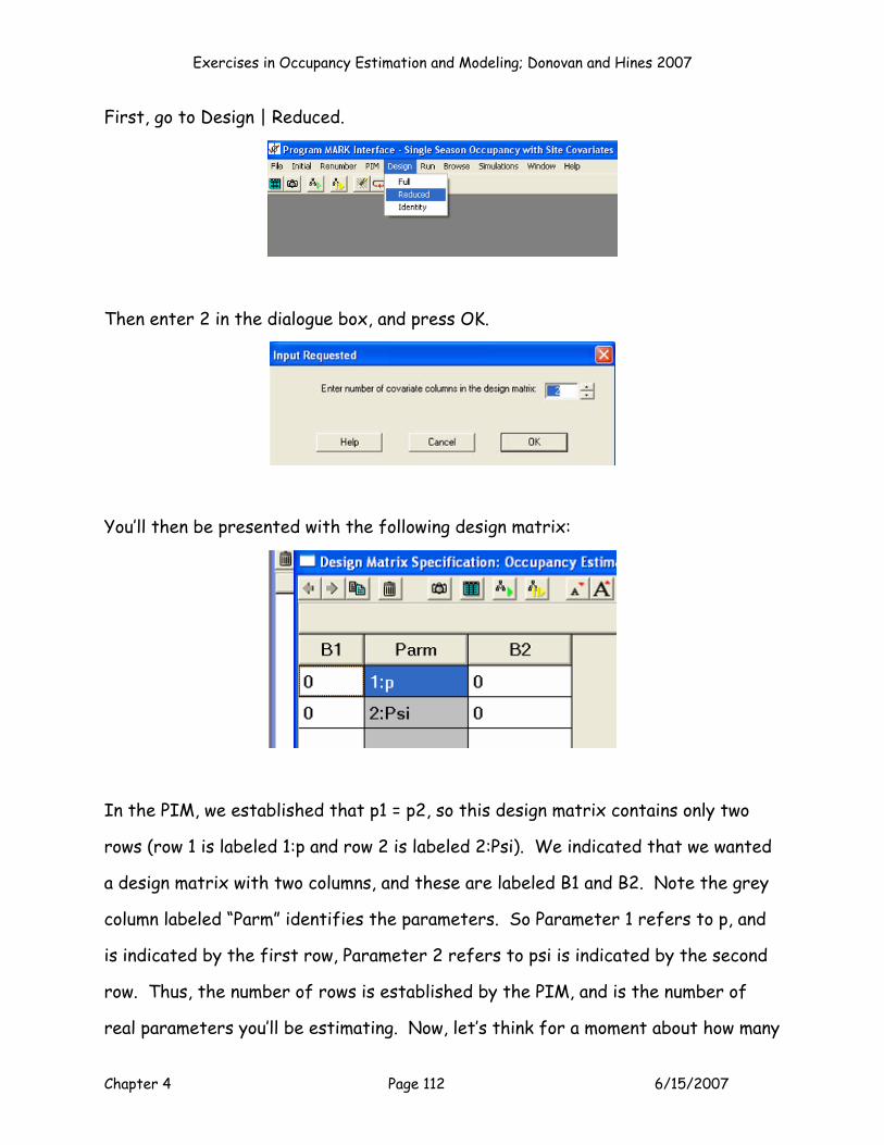
Exercises in Occupancy Estimation and Modeling; Donovan and Hines 2007
Chapter 4 Page 112 6/15/2007
First, go to Design | Reduced.
Then enter 2 in the dialogue box, and press OK.
You’ll then be presented with the following design matrix:
In the PIM, we established that p1 = p2, so this design matrix contains only two
rows (row 1 is labeled 1:p and row 2 is labeled 2:Psi). We indicated that we wanted
a design matrix with two columns, and these are labeled B1 and B2. Note the grey
column labeled “Parm” identifies the parameters. So Parameter 1 refers to p, and
is indicated by the first row, Parameter 2 refers to psi is indicated by the second
row. Thus, the number of rows is established by the PIM, and is the number of
real parameters you’ll be estimating. Now, let’s think for a moment about how many
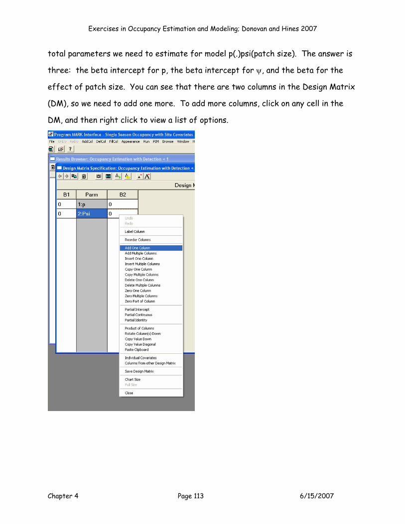
Exercises in Occupancy Estimation and Modeling; Donovan and Hines 2007
Chapter 4 Page 113 6/15/2007
total parameters we need to estimate for model p(.)psi(patch size). The answer is
three: the beta intercept for p, the beta intercept for ψ, and the beta for the
effect of patch size. You can see that there are two columns in the Design Matrix
(DM), so we need to add one more. To add more columns, click on any cell in the
DM, and then right click to view a list of options.

Exercises in Occupancy Estimation and Modeling; Donovan and Hines 2007
Chapter 4 Page 114 6/15/2007
Notice that this is an impressive list of options, but we’ll use just a couple of these
options in this exercise. Select the option labeled “Add One Column.” You should
now see a new DM:
What now? Well, we need to simply specify the linear model for each parameter.
That is, we’ll need to specify the value for the intercept for p, and we’ll need to
specify the value for the intercept and value for patch size to modify psi. Here’s
where we’re headed:

Exercises in Occupancy Estimation and Modeling; Donovan and Hines 2007
Chapter 4 Page 115 6/15/2007
In this DM, we indicate in row 1 that p (or rather, logit p) is a function of its
intercept (B1), and we indicate in row 2 that psi (or rather, logit psi) is a function
of its intercept (B2) plus patch size (B3 * patch size). So, the number of rows in
the DM specifies the number of real parameters, and the number of columns sets
the “constraints” on how those parameters are estimated. The column headings
indicate the beta number and the name of the effect. Don’t let the assigned beta
number throw you for a loop – MARK has to identify the betas in some way, and the
number assigned is not important as long as you know what it refers to. So, how
did we build this DM?
Well, to start, indicate to MARK that we need to estimate the intercept for p by
entering a 1 in the top left cell. This corresponds to column F in the spreadsheet.
Then, indicate to MARK that we need to estimate the intercept for psi by entering
a 1 under B2 for the psi parameter. This corresponds to column G in the
spreadsheet. Then, sticking with the row for psi, right-click on the cell at the
intersection of the column labeled B3 and the row labeled psi, select the option
labeled “Individual Covariates” and you should be presented with the following
dialogue box:
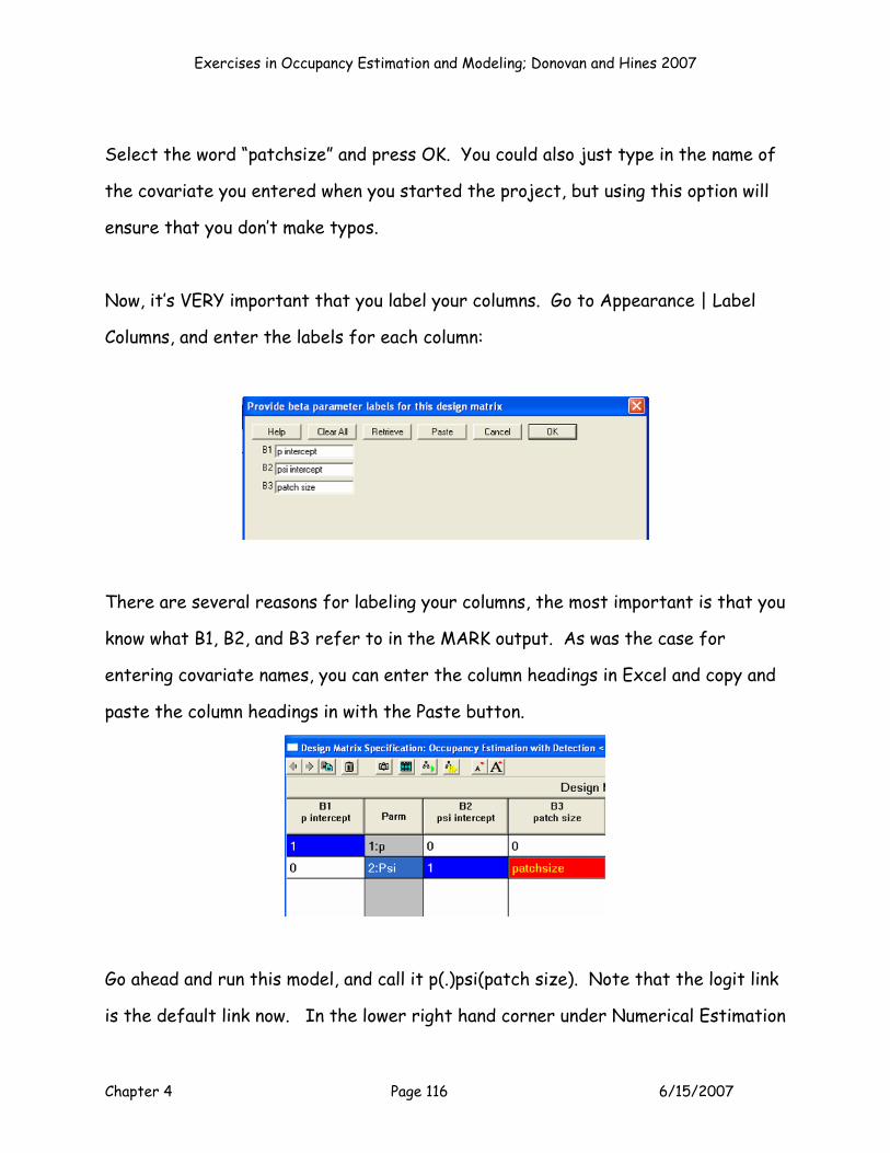
Exercises in Occupancy Estimation and Modeling; Donovan and Hines 2007
Chapter 4 Page 116 6/15/2007
Select the word “patchsize” and press OK. You could also just type in the name of
the covariate you entered when you started the project, but using this option will
ensure that you don’t make typos.
Now, it’s VERY important that you label your columns. Go to Appearance | Label
Columns, and enter the labels for each column:
There are several reasons for labeling your columns, the most important is that you
know what B1, B2, and B3 refer to in the MARK output. As was the case for
entering covariate names, you can enter the column headings in Excel and copy and
paste the column headings in with the Paste button.
Go ahead and run this model, and call it p(.)psi(patch size). Note that the logit link
is the default link now. In the lower right hand corner under Numerical Estimation
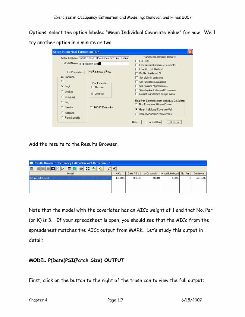
Exercises in Occupancy Estimation and Modeling; Donovan and Hines 2007
Chapter 4 Page 117 6/15/2007
Options, select the option labeled “Mean Individual Covariate Value” for now. We’ll
try another option in a minute or two.
Add the results to the Results Browser.
Note that the model with the covariates has an AICc weight of 1 and that No. Par
(or K) is 3. If your spreadsheet is open, you should see that the AICc from the
spreadsheet matches the AICc output from MARK. Let’s study this output in
detail:
MODEL P(Date)PSI(Patch Size) OUTPUT
First, click on the button to the right of the trash can to view the full output:
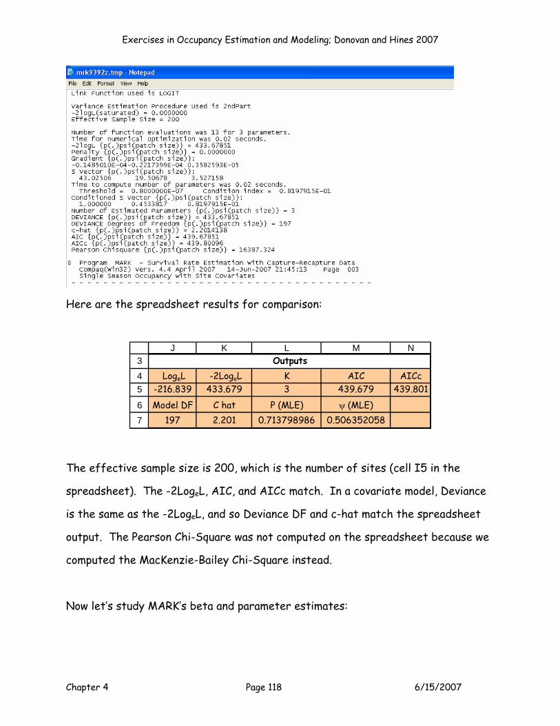
Exercises in Occupancy Estimation and Modeling; Donovan and Hines 2007
Chapter 4 Page 118 6/15/2007
Here are the spreadsheet results for comparison:
3
45
67
J K L M N
LogeL -2LogeL K AIC AICc-216.839 433.679 3 439.679 439.801Model DF C hat P (MLE) ψ (MLE)
197 2.201 0.713798986 0.506352058
Outputs
The effective sample size is 200, which is the number of sites (cell I5 in the
spreadsheet). The -2LogeL, AIC, and AICc match. In a covariate model, Deviance
is the same as the -2LogeL, and so Deviance DF and c-hat match the spreadsheet
output. The Pearson Chi-Square was not computed on the spreadsheet because we
computed the MacKenzie-Bailey Chi-Square instead.
Now let’s study MARK’s beta and parameter estimates:
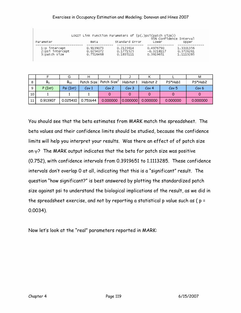
Exercises in Occupancy Estimation and Modeling; Donovan and Hines 2007
Chapter 4 Page 119 6/15/2007
8
9
10
11
F G H I J K L MB0 B00 Patch Size Patch Size2 Habitat 1 Habitat 2 PS*Hab1 PS*Hab2
P (Int) Psi (Int) Cov 1 Cov 2 Cov 3 Cov 4 Cov 5 Cov 61 1 1 0 0 0 0 0
0.913907 0.025410 0.751644 0.000000 0.000000 0.000000 0.000000 0.000000
You should see that the beta estimates from MARK match the spreadsheet. The
beta values and their confidence limits should be studied, because the confidence
limits will help you interpret your results. Was there an effect of of patch size
on ψ? The MARK output indicates that the beta for patch size was positive
(0.752), with confidence intervals from 0.3919651 to 1.1113285. These confidence
intervals don’t overlap 0 at all, indicating that this is a “significant” result. The
question “how significant?” is best answered by plotting the standardized patch
size against psi to understand the biological implications of the result, as we did in
the spreadsheet exercise, and not by reporting a statistical p value such as ( p =
0.0034).
Now let’s look at the “real” parameters reported in MARK:
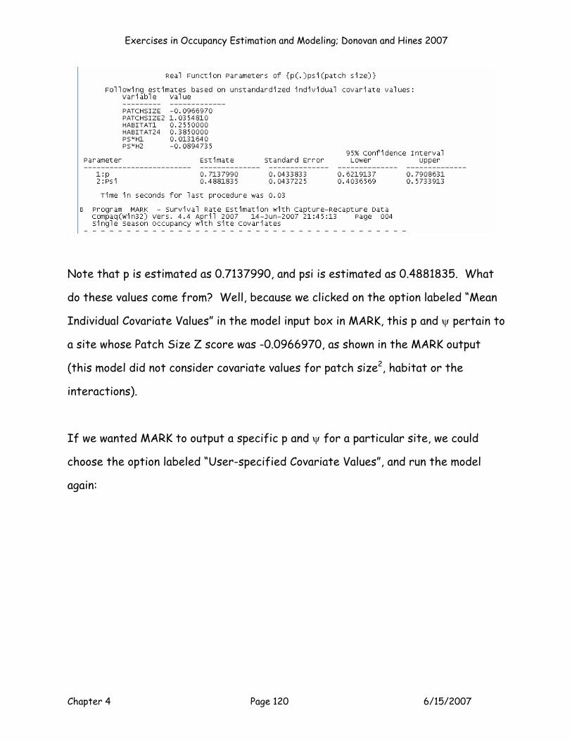
Exercises in Occupancy Estimation and Modeling; Donovan and Hines 2007
Chapter 4 Page 120 6/15/2007
Note that p is estimated as 0.7137990, and psi is estimated as 0.4881835. What
do these values come from? Well, because we clicked on the option labeled “Mean
Individual Covariate Values” in the model input box in MARK, this p and ψ pertain to
a site whose Patch Size Z score was -0.0966970, as shown in the MARK output
(this model did not consider covariate values for patch size2, habitat or the
interactions).
If we wanted MARK to output a specific p and ψ for a particular site, we could
choose the option labeled “User-specified Covariate Values”, and run the model
again:
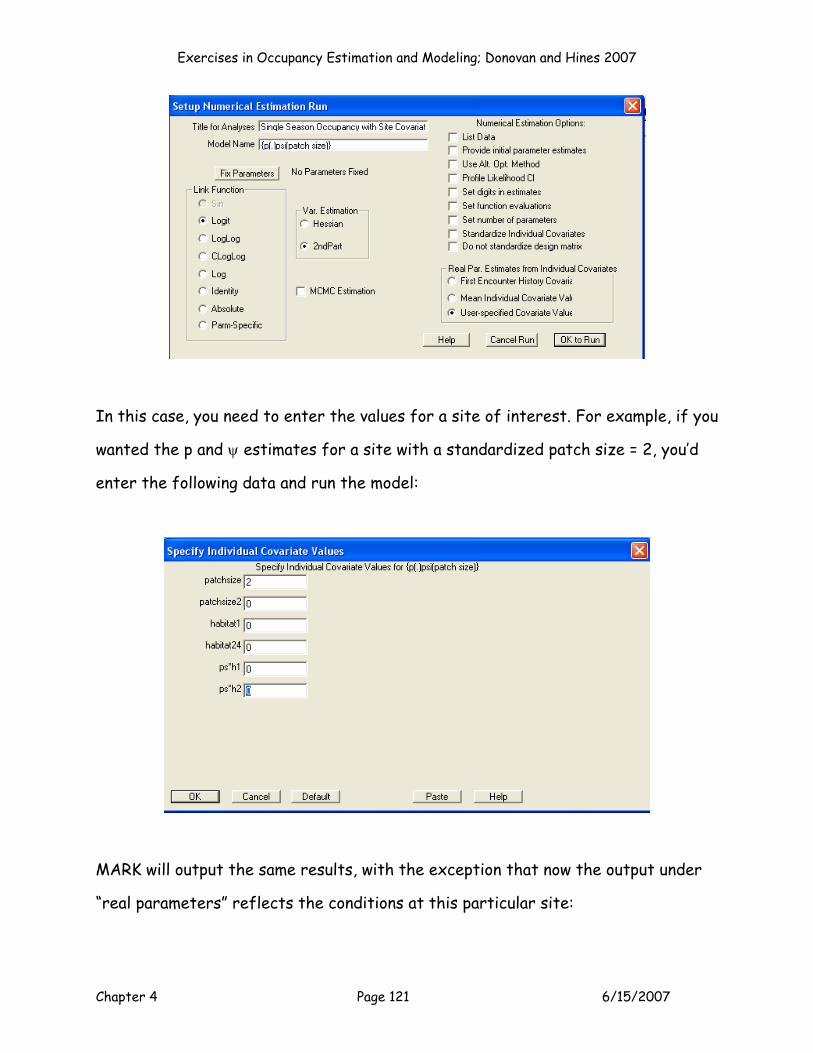
Exercises in Occupancy Estimation and Modeling; Donovan and Hines 2007
Chapter 4 Page 121 6/15/2007
In this case, you need to enter the values for a site of interest. For example, if you
wanted the p and ψ estimates for a site with a standardized patch size = 2, you’d
enter the following data and run the model:
MARK will output the same results, with the exception that now the output under
“real parameters” reflects the conditions at this particular site:
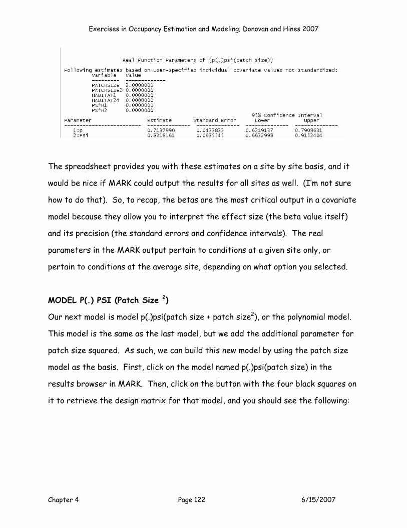
Exercises in Occupancy Estimation and Modeling; Donovan and Hines 2007
Chapter 4 Page 122 6/15/2007
The spreadsheet provides you with these estimates on a site by site basis, and it
would be nice if MARK could output the results for all sites as well. (I’m not sure
how to do that). So, to recap, the betas are the most critical output in a covariate
model because they allow you to interpret the effect size (the beta value itself)
and its precision (the standard errors and confidence intervals). The real
parameters in the MARK output pertain to conditions at a given site only, or
pertain to conditions at the average site, depending on what option you selected.
MODEL P(.) PSI (Patch Size 2)
Our next model is model p(.)psi(patch size + patch size2), or the polynomial model.
This model is the same as the last model, but we add the additional parameter for
patch size squared. As such, we can build this new model by using the patch size
model as the basis. First, click on the model named p(.)psi(patch size) in the
results browser in MARK. Then, click on the button with the four black squares on
it to retrieve the design matrix for that model, and you should see the following:
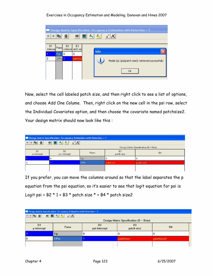
Exercises in Occupancy Estimation and Modeling; Donovan and Hines 2007
Chapter 4 Page 123 6/15/2007
Now, select the cell labeled patch size, and then right click to see a list of options,
and choose Add One Colume. Then, right click on the new cell in the psi row, select
the Individual Covariates option, and then choose the covariate named patchsize2.
Your design matrix should now look like this :
If you prefer, you can move the columns around so that the label separates the p
equation from the psi equation, so it’s easier to see that logit equation for psi is
Logit psi = B2 * 1 + B3 * patch size * + B4 * patch size2

Exercises in Occupancy Estimation and Modeling; Donovan and Hines 2007
Chapter 4 Page 124 6/15/2007
That’s all there is to it. Run this model by clicking on the button with the small
green arrow, and add the results to the results browser. Don’t forget to name the
model p(.)psi(patch size + patch size2) :
Examine the output of this model by selecting the model name in the results
browser, and then select the button to the right of the garbabe can :
The results are consistent with the spreadsheet results from this model :

Exercises in Occupancy Estimation and Modeling; Donovan and Hines 2007
Chapter 4 Page 125 6/15/2007
3
45
67
8
9
10
11
E F G H I J K L M N
11 10 01 00 Total LogeL -2LogeL K AIC AICc50 18 22 110 200 -216.556 433.112 4 441.112 441.317
Model DF C hat P (MLE) ψ (MLE)196 2.210 0.713983847 0.528851751
B0 B00 Patch Size Patch Size2 Habitat 1 Habitat 2 PS*Hab1 PS*Hab2Parameter P (Int) Psi (Int) Cov 1 Cov 2 Cov 3 Cov 4 Cov 5 Cov 6Estimate? 1 1 1 1 0 0 0 0
Beta 0.914812 0.115535 0.731197 -0.111534 0.000000 0.000000 0.000000 0.000000
Summarized Inputs Outputs
MODEL P(.) PSI(Habitat)
Now, let’s run model p(.)psi(habitat). Start by setting up the Design Matrix with
just two columns (the dot model). Go to Design | Reduced, and enter 2 for number
of betas. Now, think about how many additional parameters you need to estimate
to constrain psi to be a function of habitat. With three habitats, you must
estimate 2 additional parameters. So right click somewhere in the design matrix
and add two columns. Then, right click on the new cells in the psi row, select the
individual covariates option, and add the name of the covariates to build the model:
Your design matrix should look like this (except that you probably spelled habitat2
correctly!)
Let’s think about what this DM specifies. First, there are two rows: the top row is
where you constrain p to be a function of its intercept. The second row is where
you constrain ψ to be a function of its intercept, habitat1, and habitat2. The
intercept is B2, and pertains to sites in the reference category. Remember that
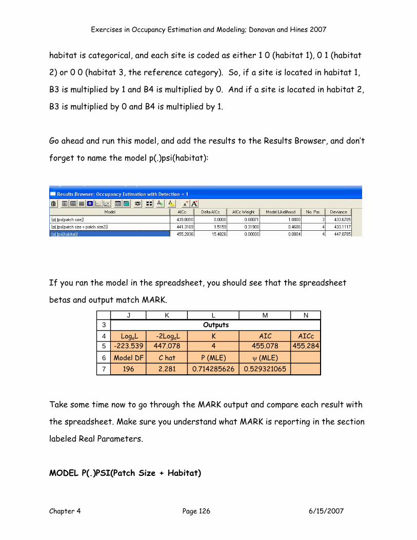
Exercises in Occupancy Estimation and Modeling; Donovan and Hines 2007
Chapter 4 Page 126 6/15/2007
habitat is categorical, and each site is coded as either 1 0 (habitat 1), 0 1 (habitat
2) or 0 0 (habitat 3, the reference category). So, if a site is located in habitat 1,
B3 is multiplied by 1 and B4 is multiplied by 0. And if a site is located in habitat 2,
B3 is multiplied by 0 and B4 is multiplied by 1.
Go ahead and run this model, and add the results to the Results Browser, and don’t
forget to name the model p(.)psi(habitat):
If you ran the model in the spreadsheet, you should see that the spreadsheet
betas and output match MARK.
3
45
67
J K L M N
LogeL -2LogeL K AIC AICc-223.539 447.078 4 455.078 455.284Model DF C hat P (MLE) ψ (MLE)
196 2.281 0.714285626 0.529321065
Outputs
Take some time now to go through the MARK output and compare each result with
the spreadsheet. Make sure you understand what MARK is reporting in the section
labeled Real Parameters.
MODEL P(.)PSI(Patch Size + Habitat)
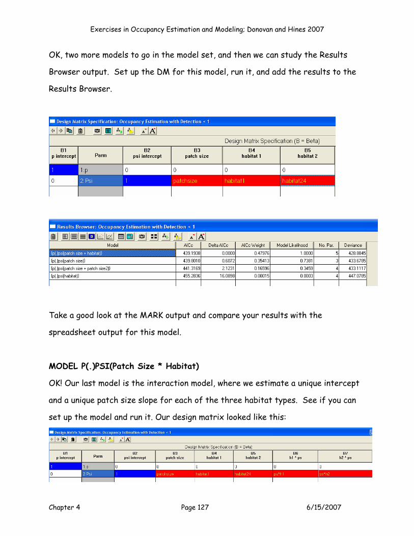
Exercises in Occupancy Estimation and Modeling; Donovan and Hines 2007
Chapter 4 Page 127 6/15/2007
OK, two more models to go in the model set, and then we can study the Results
Browser output. Set up the DM for this model, run it, and add the results to the
Results Browser.
Take a good look at the MARK output and compare your results with the
spreadsheet output for this model.
MODEL P(.)PSI(Patch Size * Habitat)
OK! Our last model is the interaction model, where we estimate a unique intercept
and a unique patch size slope for each of the three habitat types. See if you can
set up the model and run it. Our design matrix looked like this:
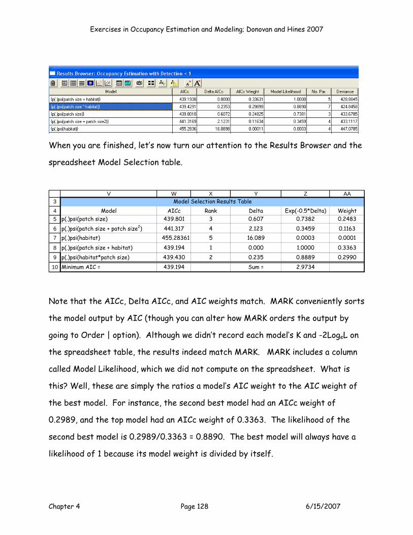
Exercises in Occupancy Estimation and Modeling; Donovan and Hines 2007
Chapter 4 Page 128 6/15/2007
When you are finished, let’s now turn our attention to the Results Browser and the
spreadsheet Model Selection table.
3
45
67
8
9
10
V W X Y Z AA
Model AICc Rank Delta Exp(-0.5*Delta) Weightp(.)psi(patch size) 439.801 3 0.607 0.7382 0.2483p(.)psi(patch size + patch size2) 441.317 4 2.123 0.3459 0.1163p(.)psi(habitat) 455.28361 5 16.089 0.0003 0.0001
p(.)psi(patch size + habitat) 439.194 1 0.000 1.0000 0.3363p(.)psi(habitat*patch size) 439.430 2 0.235 0.8889 0.2990Minimum AIC = 439.194 Sum = 2.9734
Model Selection Results Table
Note that the AICc, Delta AICc, and AIC weights match. MARK conveniently sorts
the model output by AIC (though you can alter how MARK orders the output by
going to Order | option). Although we didn’t record each model’s K and -2LogeL on
the spreadsheet table, the results indeed match MARK. MARK includes a column
called Model Likelihood, which we did not compute on the spreadsheet. What is
this? Well, these are simply the ratios a model’s AIC weight to the AIC weight of
the best model. For instance, the second best model had an AICc weight of
0.2989, and the top model had an AICc weight of 0.3363. The likelihood of the
second best model is 0.2989/0.3363 = 0.8890. The best model will always have a
likelihood of 1 because its model weight is divided by itself.

Exercises in Occupancy Estimation and Modeling; Donovan and Hines 2007
Chapter 4 Page 129 6/15/2007
MODEL AVERAGING
In the spreadsheet exercise, we briefly mentioned how to obtain model averaged
parameter estimates for each site. The method that makes the most sense for
models with individual covariates is to run a model, obtain a p and ψ estimate for
each site, and then multiply the site-specific p and ψ by the AICc weight for that
model. Then repeat this process for the remaining models in the model set, and
add up the weighted p’s and ψ’s on a site-by-site basis. This would be very easy to
do in the spreadsheet (and we probably should have added it to the exercise). I’m
not sure how to do this in MARK, although model averaging is programmed and can
be accessed by going to Output | Model Averaging.
CLOSING REMARKS
That’s it for the covariate exercise and the introduction to the Design Matrix in
MARK. In the words of Obi-Wan Kenobi, “you’ve taken your first steps into a
larger world.” Hopefully you now understand how MARK is generating parameter
estimates when covariates are used to constrain a parameter. The Design Matrix
takes time to learn, but it is well worth the time because you can constrain ANY
parameter to be a linear combination of different variables. The chapter on Linear
Constraints in MARK: A Gentle Introduction has an excellent discussion of how to
implement various kinds of models in the Design Matrix.