1

Exercise 2: Building a Watershed Base Map

Prepared by David R. Maidment and David G. Tarboton

18 September 2018, Corrected 25 September 2018

Table of Contents

Goals of the Exercise

Computer and Data Requirements

Procedure for the Assignment

1. Getting started

2. Selecting the Watersheds in the San Marcos Basin

3. Creating a San Marcos Basin Boundary

4. Land cover information for the San Marcos Basin

5. Obtaining the San Marcos Flowlines and Catchments

6. Creating a Point Feature Class of Stream Gages

7. Flow Data for the Blanco River

Summary of items to be turned in

Goals of the Exercise This exercise is intended for you to build a base data set of geographic information for a watershed using

the San Marcos Basin in South Texas as an example. The base dataset comprises watershed boundaries

and streams from the National Hydrography Dataset Plus (NHDPlus). In addition, you will create a point

Feature Class of stream gage sites by inputting latitude and longitude values for the gages in an Excel

table that is added to ArcMap and the geodatabase. You will create a resource in Hydroshare of the San

Marcos Basin and use it as a backdrop to download forecasts from the National Water Model.

Computer and Data Requirements To complete this exercise, you'll need to run ArcGIS Pro version 2.2 from a PC. You will download

hydrologic information to do this exercise from HydroShare and other online data sources.

Procedure for the Assignment

Getting Started

We’ll begin by getting the input data for Water Resource Region 12, and creating a new, empty

geodatabase into which you’ll put data for the San Marcos basin, which is a small drainage area within

this region.

2

Open the ArcGIS Online map at: http://arcg.is/1JW0DBm This map is publicly shared so you don’t need

to login to ArcGIS Online to use it. Click on the Texas Gulf region. If there is no response, try another

browser.

Then click on More info

And scroll down to Content

Download the file NFIEGeo_12.gdb.zip (127.1MB). If you have trouble locating this file, you can get it

directly at:

https://www.hydroshare.org/resource/1d78964652034876b1c190647b21a77d/

Unzip this file and navigate down through the folders to a zipped geodatabase file, and unzip that. Move

the geodatabase file to your working directory for this exercise. NFIE stands for National Flood

Interoperability Experiment, which was the academic effort that we undertook to establish the prototype

for the National Water Model. NFIEGeo is the geospatial database that we created to support this effort,

and NFIEGeo_12 is the portion of that geodatabase that covers USGS Water Resources Region 12, the

3

rivers and streams that drain to the Texas Gulf Coast. NFIEGeo_12.gdb is a geodatabase containing this

information.

Open ArcGIS Pro and create a new Blank Project for this exercise. I have called this Exercise2. It’s a

good idea to just use one word titles for projects because this is the name of the Geodatabase that you

create within the project. In general, ArcGIS likes to have single word titles as the names for things or

otherwise you have to interpret spaces and that can be ambiguous.

Insert a New Map into your view

And you’ll see a big topographic map of the United States show up.

Add the NFIEGeo_12 data to the map by using the Add Data button and navigating to the Feature

Dataset Geographic. A feature dataset is a folder that contains feature classes all having the same spatial

reference or geographic coordinate system.

4

This adds all the feature classes in this feature dataset to your map view.

5

You’ll see that there are five feature classes in this Geographic feature dataset. Turn off the display of all

feature classes except for Subwatershed and recolor the Subwatersheds using the HUC_8 attribute using

Unique Values. Right Click on the Subwatershed feature class and select Symbology

and in the Symbology window that opens on the right hand side click on the Single Symbol bar and

change this to Unique Values

And select HUC_8 as the Field to be used to display these values

6

You’ll be asked a question as to whether you want more than 100 Unique values, and answer Yes to this

question.

Your resulting map should look something like this (the colors may be different on your map). The

different colors represent HUC8 Subbasins and the outlines are HUC12 Subwatersheds. You can change

the default color scheme that you get by clicking on Color scheme in the Symbology window and

selecting a new one.

Use Project/Save to save the current version of your project so you don’t have to recreate this map

display again. The project is saved in a file Exercise2.aprx, in the folder Exercise2.

At the bottom of the Right Pane, click on the Catalog tab to open the Catalog window

7

If you open up the Databases section of the Catalog display, you’ll see a new Geodatabase already created

for you called Exercise2.gdb, consistent with the name of the Project that we created when opening

ArcGIS Pro.

Right click on this Exercise2.gdb Geodatabase and create a new Feature Dataset.

Call this new dataset SanMarcos (again, just use one word titles for files) and select the coordinate

system for the Subwatershed class you are working with. This is a geographic coordinate system defined

on the NAD83 datum, or North American Datum of 1983: GCS_North_American_1983.

8

Hit Run at the bottom of the tab to execute this action. Notice that you are in a new Tab now called

Geoprocessing, which indicates that you are creating new information.

If you go back to the Catalog pane, and expand the Exercise2 geodatabase, you’ll see its got a

SanMarcos feature dataset inside it now, which will hold the data that you create for the San Marcos

Basin.

9

Selecting the Watersheds in the San Marcos Basin

Let’s focus on data in the San Marcos basin. The Subwatersheds feature class is a part of the Watershed

Boundary Dataset of the United States, which subdivides the nation’s drainage into a hierarchy of

drainage areas. https://www.usgs.gov/core-science-systems/ngp/national-hydrography/watershed-

boundary-dataset We want all the HUC12 subwatersheds that lie within the San Marcos subbasin, which

has a HUC8 value of 12100203; these are the first 8 digits of the HUC12 identifier. This means that these

drainage areas lie within Region 12, Subregion 10, Basin 02 and Subbasin 03.

Open the Attribute Table of the Subwatershed feature class by right clicking on the Subwatershed in the

Map view and selecting Attribute Table

A window like this will open up in your map display.

Now let’s select some records in this table that describe the San Marcos Basin. In the Table View, menu

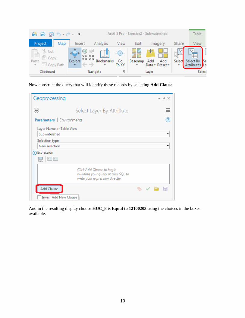
at the top choose Select by Attributes

10

Now construct the query that will identify these records by selecting Add Clause

And in the resulting display choose HUC_8 is Equal to 12100203 using the choices in the boxes

available.

11

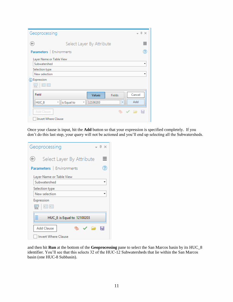
Once your clause is input, hit the Add button so that your expression is specified completely. If you

don’t do this last step, your query will not be actioned and you’ll end up selecting all the Subwatersheds.

and then hit Run at the bottom of the Geoprocessing pane to select the San Marcos basin by its HUC_8

identifier. You’ll see that this selects 32 of the HUC-12 Subwatersheds that lie within the San Marcos

basin (one HUC-8 Subbasin).

12

If you hit the Show Selected Records button at the bottom of the Table, you’ll see the selected records,

and also their highlighted images in the map.

To zoom to this selection, use the Zoom to Selected Features button in the map tab.

And you’ll see a close up view of the San Marcos Subwatersheds.

13

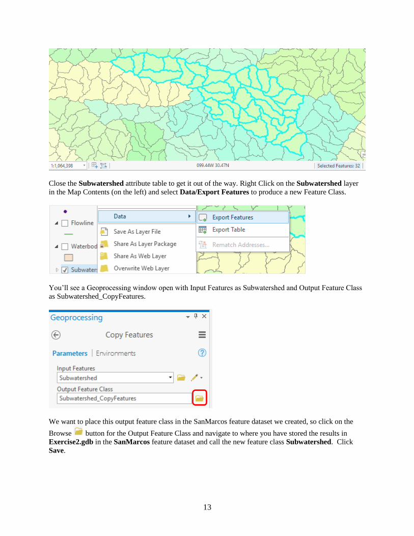
Close the Subwatershed attribute table to get it out of the way. Right Click on the Subwatershed layer

in the Map Contents (on the left) and select Data/Export Features to produce a new Feature Class.

You’ll see a Geoprocessing window open with Input Features as Subwatershed and Output Feature Class

as Subwatershed_CopyFeatures.

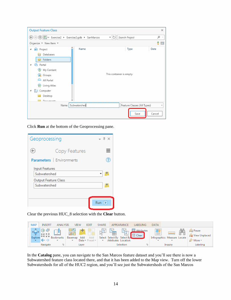
We want to place this output feature class in the SanMarcos feature dataset we created, so click on the

Browse button for the Output Feature Class and navigate to where you have stored the results in

Exercise2.gdb in the SanMarcos feature dataset and call the new feature class Subwatershed. Click

Save.

14

Click Run at the bottom of the Geoprocessing pane.

Clear the previous HUC_8 selection with the Clear button.

In the Catalog pane, you can navigate to the San Marcos feature dataset and you’ll see there is now a

Subwatershed feature class located there, and that it has been added to the Map view. Turn off the lower

Subwatersheds for all of the HUC2 region, and you’ll see just the Subwatersheds of the San Marcos

15

basin. Pretty cool! We’ve just taken a large dataset and selected from that a smaller dataset of interest for

our study.

Remove the larger Subwatershed feature class for all of the Region 12 by right clicking on it and selecting

Remove

Note that in ArcGIS there is generally a distinction between Remove and Delete. Remove is a safe action

that detaches a data set from a document. Delete is a less safe action, it actually deletes the object from

disk.

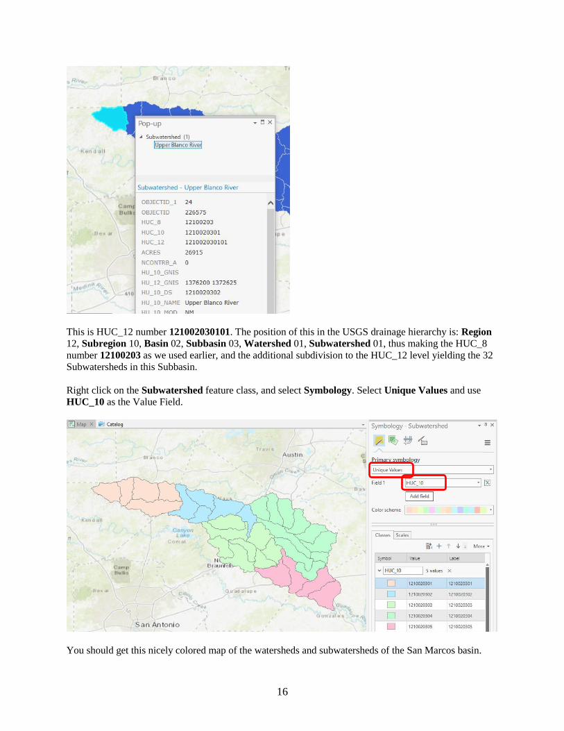
Click on the North-Western subwatershed on the map.

16

This is HUC_12 number 121002030101. The position of this in the USGS drainage hierarchy is: Region

12, Subregion 10, Basin 02, Subbasin 03, Watershed 01, Subwatershed 01, thus making the HUC_8

number 12100203 as we used earlier, and the additional subdivision to the HUC_12 level yielding the 32

Subwatersheds in this Subbasin.

Right click on the Subwatershed feature class, and select Symbology. Select Unique Values and use

HUC_10 as the Value Field.

You should get this nicely colored map of the watersheds and subwatersheds of the San Marcos basin.

17

Notice that the 32 HUC-12 subwatersheds have been grouped into five watersheds within the San Marcos

subbasin (I am here using the Watershed Boundary Dataset nomenclature to refer to the drainage area

hierarchy in its formal sense).

Use Project/Save to update your Exercise2.aprx map project with the new information that you’ve

created.

Where is My Stuff?

Right click on Subwatershed and select Properties and select the Source tab. Notice that this Feature

Class you created is in the SanMarcos Feature Dataset in the Exercise2.gdb Geodatabase in the location

where you created it. It comprises Simple Features (no topology) that are Polygons (have X and Y values)

but have no Z or M values, which deal with elevation and measure, respectively.

If you look at your Exercise2 folder on disk that was created when you created the project you will see a

number of files, including Exercise2.gdb, which is the folder that holds this data in File Geodatabase

format.

18

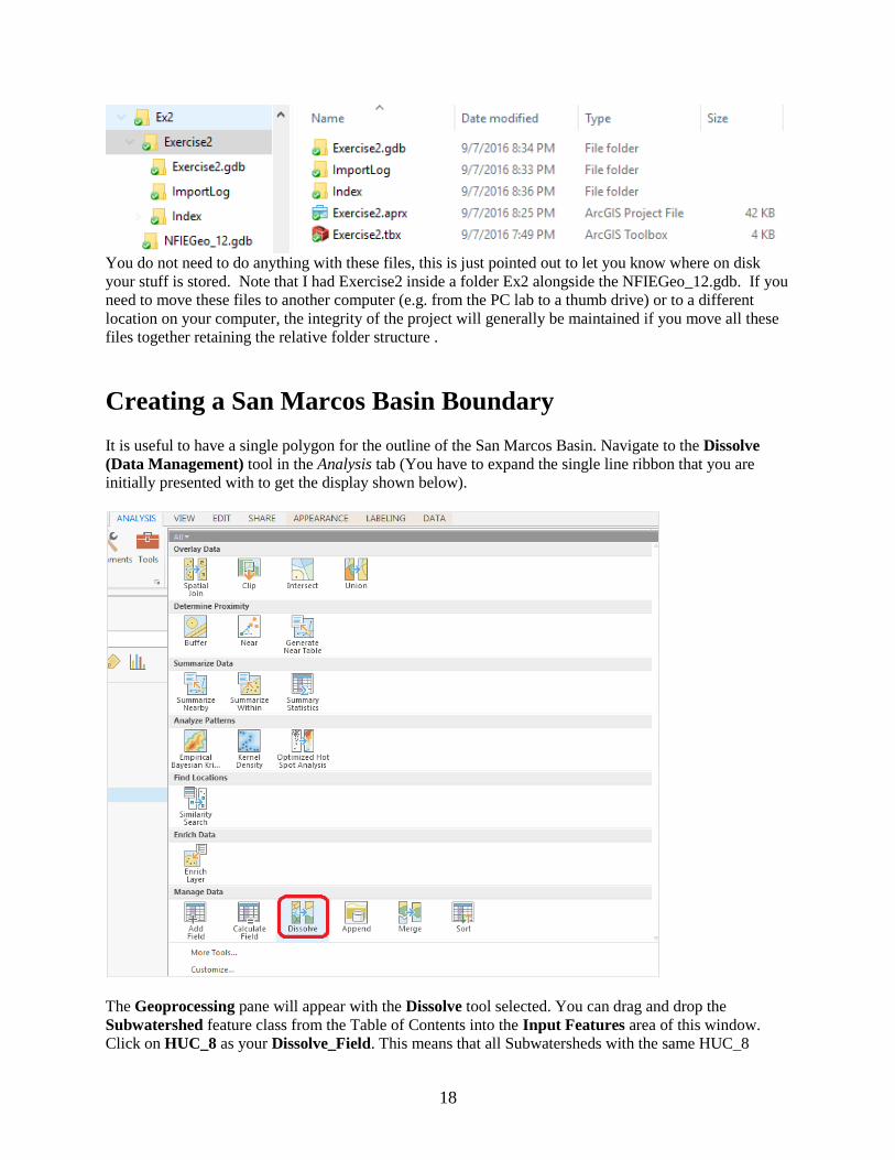
You do not need to do anything with these files, this is just pointed out to let you know where on disk

your stuff is stored. Note that I had Exercise2 inside a folder Ex2 alongside the NFIEGeo_12.gdb. If you

need to move these files to another computer (e.g. from the PC lab to a thumb drive) or to a different

location on your computer, the integrity of the project will generally be maintained if you move all these

files together retaining the relative folder structure .

Creating a San Marcos Basin Boundary

It is useful to have a single polygon for the outline of the San Marcos Basin. Navigate to the Dissolve

(Data Management) tool in the Analysis tab (You have to expand the single line ribbon that you are

initially presented with to get the display shown below).

The Geoprocessing pane will appear with the Dissolve tool selected. You can drag and drop the

Subwatershed feature class from the Table of Contents into the Input Features area of this window.

Click on HUC_8 as your Dissolve_Field. This means that all Subwatersheds with the same HUC_8

19

number (12100203) will be merged together. Set the output Feature class to be called Basin in your

SanMarcos feature dataset. Hit Run to execute the function.

And you’ll see a new Basin feature class pop up on your map display

Navigate to the Symbology and select No Color for the shape, Green for the Outline Color and 2 for the

Outline Width.

20

You will now have a very nice looking map of the San Marcos Basin with its constituent subdrainage

areas.

Right click on the Basin feature class and open its Attribute Table. Notice that the Basin feature class has

only one Polygon and it is identified with the HUC_8 = 12100203, which is the 8-digit number all the

HUC_12 subwatersheds had in common.

Use Project/Save to save your ArcGIS Pro project. Close the attribute table for the Basin feature class.

21

Navigate to your SanMarcos feature dataset in the Project pane. Notice how you’ve now got the

Watershed and Basin feature classes that you’ve just created stored inside it.

To be turned in: Make a map of the San Marcos basin with its HUC10 and HUC12 watersheds and

subwatersheds. Use a layout as you learned in exercise 1. How many HUC10 and HUC12 units exist in

the San Marcos Basin? Note that maps that you turn in should be clearly labeled so that they may be

unambiguously interpreted with a title, scale, north arrow and appropriate legend information.

Land Cover Information for the San Marcos Basin

Now, we are going to use some of the online data services to find some land cover properties of the San

Marcos basin. Select Add Data to the Map

And among the options presented, select Living Atlas.

22

In the Search Portal: Living Atlas type in nlcd for National Land Cover Dataset, and among the options

presented, select USA NLCD Land Cover 2011

and you’ll see it shows up on the map with predetermined color scheme that highlights urban areas in red.

In the Table of Contents click off the Subwatershed layer, so that you only have the Basin displayed

over the land cover data. San Antonio is towards the bottom of the map, Austin near the top, and San

Marcos lies within the basin. Notice also the profusion of yellow and brown for Agriculture on the right-

hand side of the map, to the east of the Balcones escarpment. Forest areas predominate on the west side

of the basin.

23

Use Project/Save to save the current map display.

In the Geoprocessing pane, in the top right hand corner, select Open Another Tool

And enter Extract by Mask in the Find Tools box.

24

Click on the Extract by Mask (Spatial Analyst Tools) tool, and use USA NLCD Land Cover 2011 as

the Input Raster and Basin as the mask data; put the result in the Exercise2 geodatabase with the name

LandCover. Be careful to store the Output raster directly inside the Exercise2.gdb, not inside the

SanMarcos Feature Dataset, which only stores vector feature classes.

At the Extract by Mask step specify the output Coordinate System to be

North_America_Albers_Equal_Area.

After Setting the inputs and outputs, Click on Environments

25

Then specify the Output Coordinate System

In the layer that results, the coordinate system should be as below

Click Run.

26

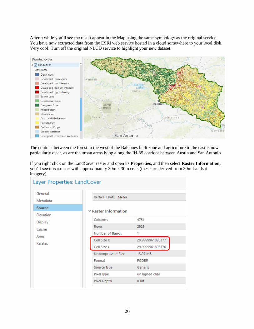
After a while you’ll see the result appear in the Map using the same symbology as the original service.

You have now extracted data from the ESRI web service hosted in a cloud somewhere to your local disk.

Very cool! Turn off the original NLCD service to highlight your new dataset.

The contrast between the forest to the west of the Balcones fault zone and agriculture to the east is now

particularly clear, as are the urban areas lying along the IH-35 corridor between Austin and San Antonio.

If you right click on the LandCover raster and open its Properties, and then select Raster Information,

you’ll see it is a raster with approximately 30m x 30m cells (these are derived from 30m Landsat

imagery).

27

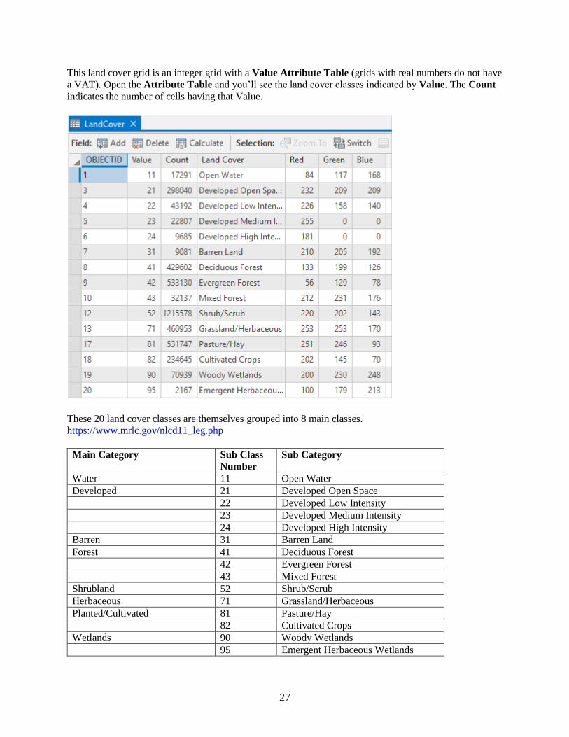
This land cover grid is an integer grid with a Value Attribute Table (grids with real numbers do not have

a VAT). Open the Attribute Table and you’ll see the land cover classes indicated by Value. The Count

indicates the number of cells having that Value.

These 20 land cover classes are themselves grouped into 8 main classes.

https://www.mrlc.gov/nlcd11_leg.php

Main Category Sub Class

Number

Sub Category

Water 11 Open Water

Developed 21 Developed Open Space

22 Developed Low Intensity

23 Developed Medium Intensity

24 Developed High Intensity

Barren 31 Barren Land

Forest 41 Deciduous Forest

42 Evergreen Forest

43 Mixed Forest

Shrubland 52 Shrub/Scrub

Herbaceous 71 Grassland/Herbaceous

Planted/Cultivated 81 Pasture/Hay

82 Cultivated Crops

Wetlands 90 Woody Wetlands

95 Emergent Herbaceous Wetlands

28

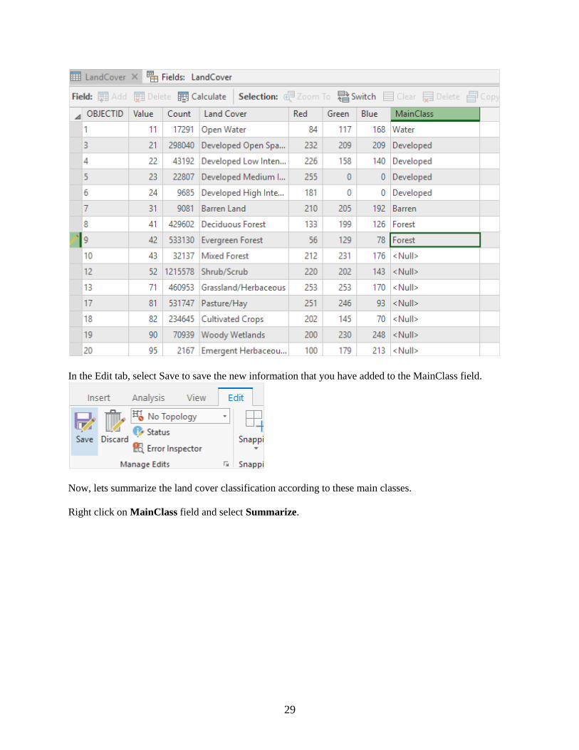
Let’s add these main classes to the Value Attribute Table for Land Cover. In the Table view menu, click

on Add to add a Field. Note that you have to have the Table active for this menu to be available.

And in the Fields: LandCover table that appears change the Field Name from Field to MainClass and the

Data Type to Text. Sometimes it takes a few clicks on these field names before they will allow you to

edit them.

Click Save at the top of the display to apply these changes.

Now, when you return to the LandCover Table, you’ll see a new Field called MainClass on the right hand

side. Initially all values will be null. Click on each row in this field and add the appropriate MainClass

title. I have only partially completed adding these values in the table below. They should all be filled in.

29

In the Edit tab, select Save to save the new information that you have added to the MainClass field.

Now, lets summarize the land cover classification according to these main classes.

Right click on MainClass field and select Summarize.

30

In the Field section select Count with a Statistic Type SUM, then save the result as a table called

LandCoverSummary in the Exercise2 geodatabase (not in the SanMarcos feature dataset). Leave the

Case field as MainClass. What this action does is to create a new table that sums the count of the cells for

all the land cover subcategories in each Main Class

Click Run. What this action does is to create a new table that sums for the San Marcos basin the count of

the cells for all the land cover subcategories in each Main Class. This table shows up in your Table of

Contents at the bottom of the display.

31

If you use the Catalog pane to navigate to Databases, you’ll see that you have a new

LandCoverSummary table in your geodatabase, along with the LandCover raster created earlier:

Use Project/Save to save your project file.

The Sum_Count of the number of grid cells in this table, can be used with cell size (30m) to determine

the area in each land cover class.

To be turned in: Make a map of the land cover over the San Marcos Basin. Prepare a table that shows

the area (km2) of each of the main land cover classes and the % of the total basin area that each land

cover class represents.

32

Obtaining the San Marcos Flowlines and Catchments

Go back to the data from NFIEGeo_12.gdb that you downloaded at the beginning of the exercise and

focus on the Flowlines and Catchment layers in to your Map display. Turn off the LandCover

distribution. If necessary, reload the Flowlines and Catchment from the geodatabase to the map display.

Color your Catchments as “No Color” with a green outline, and your Flowlines as nice blue streams using

the same procedure as before of Right Clicking on the feature class name and selecting Symbology from

the choices then available to you.

Now, let’s select the features from our large dataset that lie within our Basin. Click the Selection by

Location button on the Map tab.

33

Select the features from the Flowline feature class that Have their center in the Basin and you’ll see

these flowlines selected as shown below.

34

Right click on the Flowline feature class and select Data/Export Data to Export these selected Flowlines

to a feature class called Flowline in the SanMarcos geodatabase.

Remove the original Flowline feature class for Region 12 from your map display (it is the lower of the

two Flowline feature classes in the Table of Contents.

Repeat the same process with Catchment as you did for Flowline: (1) Use Select by Location to select

those catchments having their center in the San Marcos basin; (2) Export those catchments to the San

Marcos feature dataset as a new feature class; (3) Remove the larger Region 12 catchment set from the

map display and recolor the San Marcos catchments appropriately as a backdrop to your selected flowline

set.

Use Project/Save to save your new data display.

This map looks a little bit like spaghetti, so let’s recolor the Flowlines according to the Mean Annual

Flow (Q0001C attribute). Right click on the Flowline feature class and select Symbology. Use

Graduated Symbols

35

Using Field Q0001C (the mean annual flow of each flowline in cubic feet per second)

and click on Template to change the base color to blue.

Turn off the Catchments and you’ll get a nice display of the distribution of the streams and rivers in the

San Marcos Basin

36

Use the Locate button in the Map view to locate the town of Wimberley,

Texas

Click on the reach of the Blanco River just adjacent to Wimberley:

37

And you’ll see that this reach has a COMID = 1630223. If you click on the catchment within which this

flowline is located, you’ll see that it has a FeatureID = 1630223. It is this one to one relationship

between the COMID of the Flowline and the FeatureID of the Catchment that connects the river and

stream segments with their surrounding local drainage areas in the National Water Model.

Use Zoom to Layer for the Basin feature class to get back the original extent of our map.

38

Turn off the Locate panel to eliminate the symbolization of Wimberley.

Explore the map and identify where the Blanco River, San Marcos River and Plum Creek are located in

the basin.

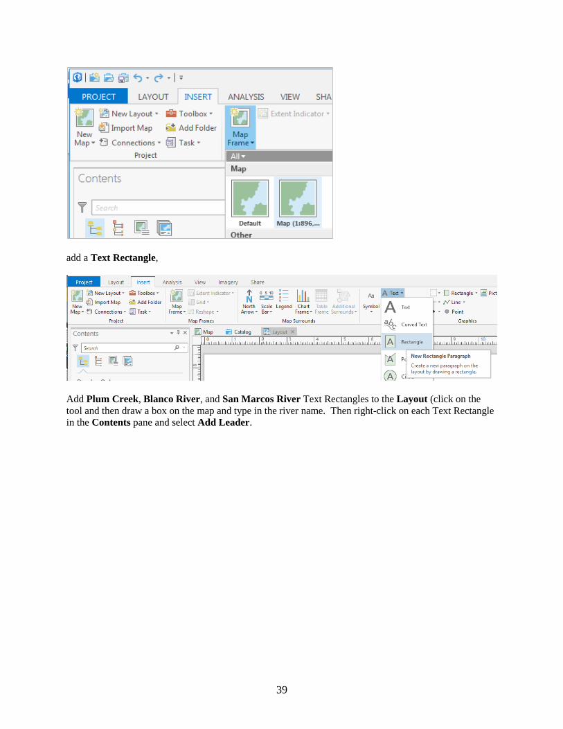
Now let’s create a map and do some summarization of watershed attributes. We’ll need to create a new

Layout with the New Layout button in the Insert tab. Use 8 ½” x 11” Portrait Letter layout option.

Add your Map Frame to the Layout (make sure you can see the whole basin),

39

add a Text Rectangle,

Add Plum Creek, Blanco River, and San Marcos River Text Rectangles to the Layout (click on the

tool and then draw a box on the map and type in the river name. Then right-click on each Text Rectangle

in the Contents pane and select Add Leader.

40

Move the Text Rectangles around and select Add Leader again to change the location of the pointer until

your map looks something like this:

41

Note that Add Leader repositions the point of the leader, so you need to use trial and error to get the text

and leader point the way you want it.

Save your map document as Ex2_project_flow.aprx to preserve your layout.

Switch back to the Map tab and open the attribute table for Flowline. Note that there is a field

LENGTHKM that was obtained from the original data. Use this to compute the average length of

flowlines. Right click on the LengthKm feature field and select Summarize

Accept the default value Flowline_Statistics as the output table. Use LengthKm as the Statistics Field

and Mean as Statistics Type. Remove LengthKm as the Case field.

42

Hit Run and you’ll see a new table at the bottom of the Table of Contents panel which gives you the

number of flowlines and their average length.

The attribute table for Catchment has a field AreaSqKM from the original data. Use this field to

similarly evaluate the average area of catchments.

Note that the fields Shape_Length and Shape_Area in these tables should not be used for length and area

as they are in geographic coordinates so do not account for the curvature of the earth.

To be turned in: Make a map of the San Marcos basin with its labeled rivers. How many Catchments lie

within this basin? What is their average area (Sq. Km)? How many Flowlines lie within this basin?

What is their average length (Km)?

Creating a Point Feature Class of Stream Gages

Now you are going to build a new Feature Class yourself of stream gage locations in the San Marcos

basin. I have extracted information from the USGS site information at

https://waterdata.usgs.gov/tx/nwis/inventory

SiteID SiteName Latitude Longitude DASqMile MAFlow

08171000 Blanco Rv at Wimberley, Tx

29⁰ 59'

39" 98⁰ 05' 19" 355 142

08171300 Blanco Rv nr Kyle, Tx

29⁰ 58'

45" 97⁰ 54' 35" 412 165

08172400 Plum Ck at Lockhart, Tx

29⁰ 55'

22" 97⁰ 40' 44" 112 49

08173000 Plum Ck nr Luling, Tx

29⁰ 41'

58" 97⁰ 36' 12" 309 114

08172000 San Marcos Rv at Luling, Tx

29⁰ 39'

58" 97⁰ 39' 02" 838 408

08170500 San Marcos Rv at San Marcos, Tx

29⁰ 53'

20" 97⁰ 56' 02" 48.9 176

(a) Define a table containing an ID and the long, lat coordinates of the gages

The coordinate data is in geographic degrees, minutes, & seconds. These values need to be converted to

digital degrees, so go ahead and perform that computation for the 6 pairs of longitude and latitude values.

This is something that has to be done carefully because any errors in conversions will result in the stations

lying well away from the San Marcos basin. I suggest that you prepare an Excel table showing the gage

longitude and latitude in degrees, minutes and seconds, convert it to long, lat in decimal degrees:

43

𝐷𝑒𝑐𝑖𝑚𝑎𝑙 𝐷𝑒𝑔𝑟𝑒𝑒𝑠 (𝐷𝐷) = 𝐷𝑒𝑔𝑟𝑒𝑒𝑠 + 𝑀𝑖𝑛

60 +

𝑆𝑒𝑐𝑜𝑛𝑑𝑠

3600

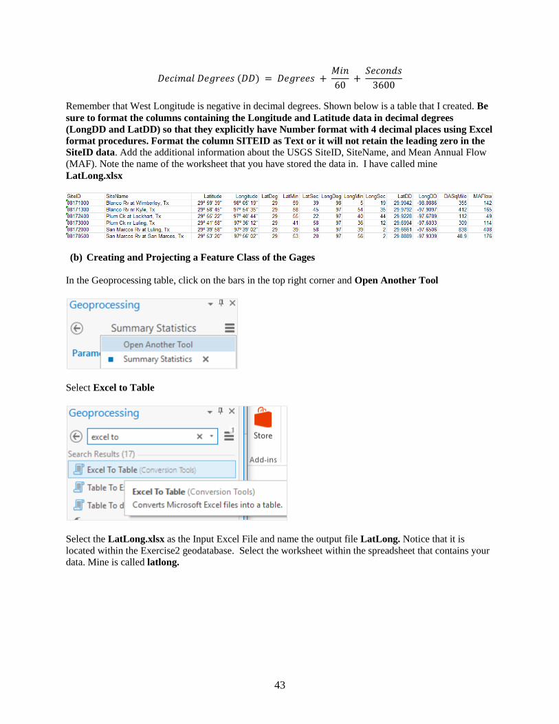
Remember that West Longitude is negative in decimal degrees. Shown below is a table that I created. Be

sure to format the columns containing the Longitude and Latitude data in decimal degrees

(LongDD and LatDD) so that they explicitly have Number format with 4 decimal places using Excel

format procedures. Format the column SITEID as Text or it will not retain the leading zero in the

SiteID data. Add the additional information about the USGS SiteID, SiteName, and Mean Annual Flow

(MAF). Note the name of the worksheet that you have stored the data in. I have called mine

LatLong.xlsx

(b) Creating and Projecting a Feature Class of the Gages

In the Geoprocessing table, click on the bars in the top right corner and Open Another Tool

Select Excel to Table

Select the LatLong.xlsx as the Input Excel File and name the output file LatLong. Notice that it is

located within the Exercise2 geodatabase. Select the worksheet within the spreadsheet that contains your

data. Mine is called latlong.

44

Click Run

Now we are going to convert the tabular data in the spreadsheet to points in the ArcGIS Pro display.

Right click on the new table, LatLong, and select Display XY Data

Set the X Field to LongDD, the Y Field to LatDD. Note that by default the GCS_WGS_1984 coordinate

system is chosen. This is incorrect for this dataset and must be changed to GCS_North_American_1983.

Name the Output Feature Class Gages and save it in the SanMarcos feature dataset

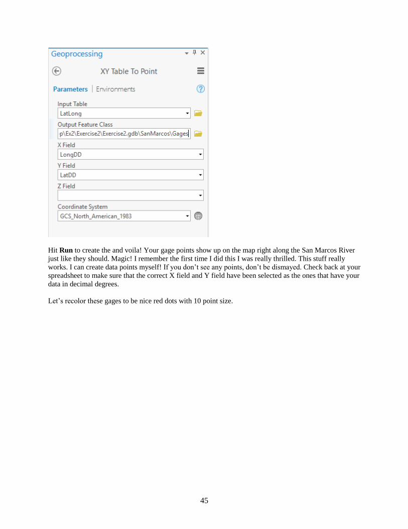
45

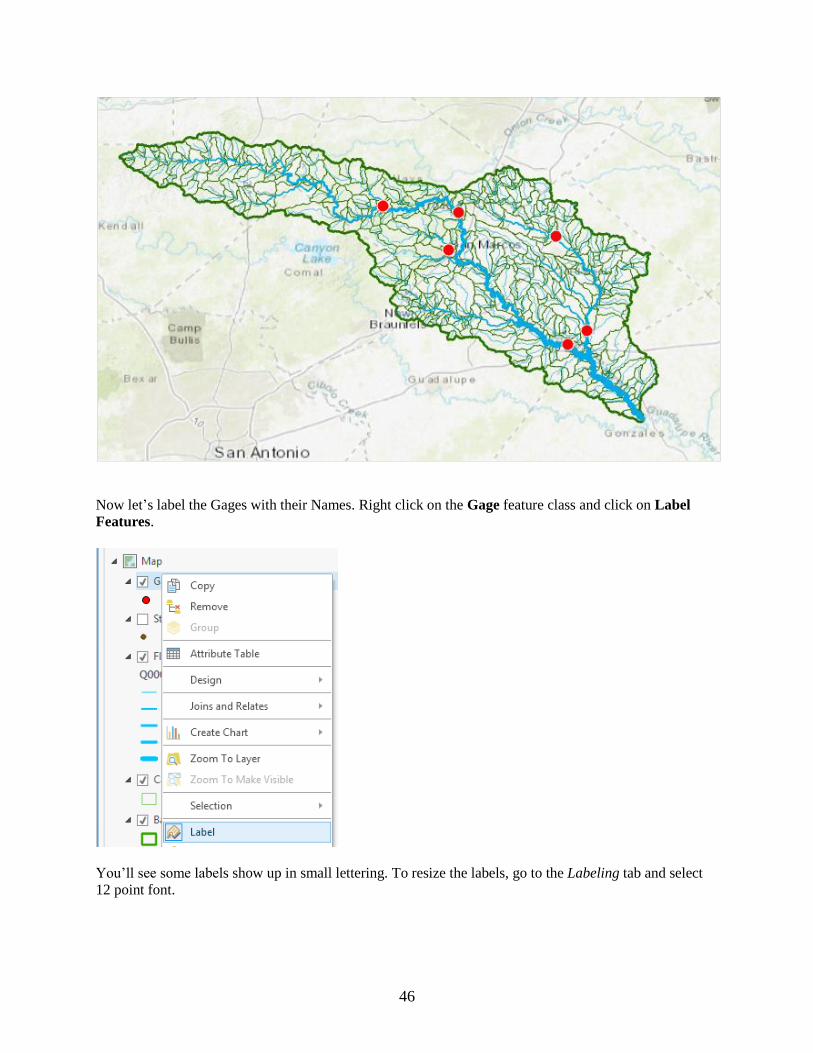
Hit Run to create the and voila! Your gage points show up on the map right along the San Marcos River

just like they should. Magic! I remember the first time I did this I was really thrilled. This stuff really

works. I can create data points myself! If you don’t see any points, don’t be dismayed. Check back at your

spreadsheet to make sure that the correct X field and Y field have been selected as the ones that have your

data in decimal degrees.

Let’s recolor these gages to be nice red dots with 10 point size.

46

Now let’s label the Gages with their Names. Right click on the Gage feature class and click on Label

Features.

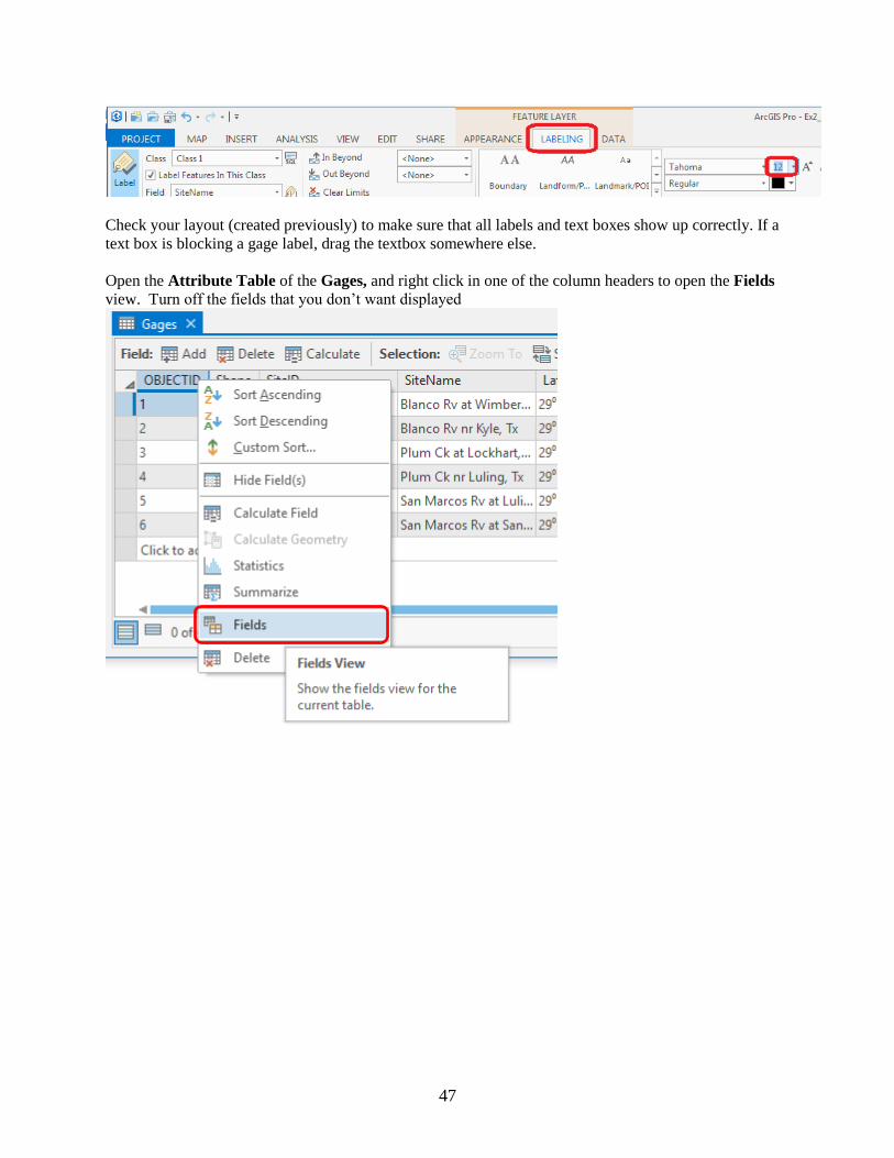
You’ll see some labels show up in small lettering. To resize the labels, go to the Labeling tab and select

12 point font.

47

Check your layout (created previously) to make sure that all labels and text boxes show up correctly. If a

text box is blocking a gage label, drag the textbox somewhere else.

Open the Attribute Table of the Gages, and right click in one of the column headers to open the Fields

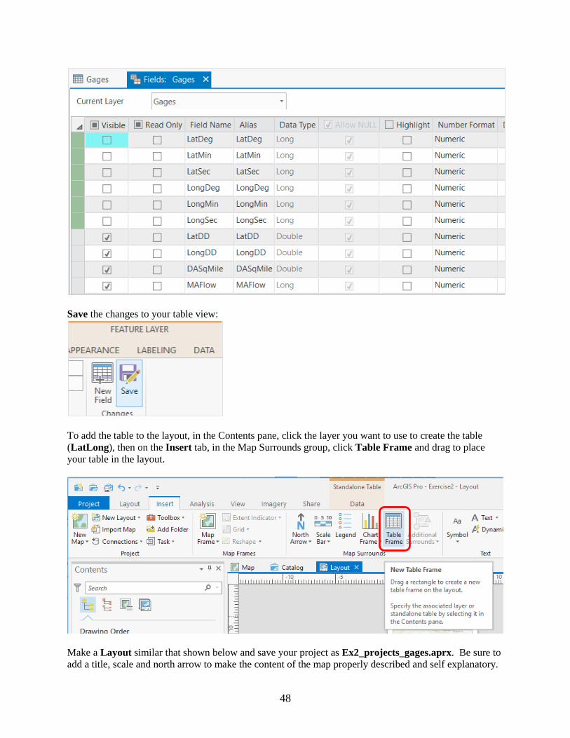
view. Turn off the fields that you don’t want displayed

48

Save the changes to your table view:

To add the table to the layout, in the Contents pane, click the layer you want to use to create the table

(LatLong), then on the Insert tab, in the Map Surrounds group, click Table Frame and drag to place

your table in the layout.

Make a Layout similar that shown below and save your project as Ex2_projects_gages.aprx. Be sure to

add a title, scale and north arrow to make the content of the map properly described and self explanatory.

49

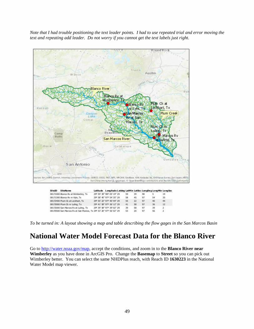
Note that I had trouble positioning the text leader points. I had to use repeated trial and error moving the

text and repeating add leader. Do not worry if you cannot get the text labels just right.

To be turned in: A layout showing a map and table describing the flow gages in the San Marcos Basin

National Water Model Forecast Data for the Blanco River

Go to http://water.noaa.gov/map, accept the conditions, and zoom in to the Blanco River near

Wimberley as you have done in ArcGIS Pro. Change the Basemap to Street so you can pick out

Wimberley better. You can select the same NHDPlus reach, with Reach ID 1630223 in the National

Water Model map viewer.

50

Use Open Forecast Chart to get the forecast data for the Analysis and Short Range models. Click

on the Medium Range model and select Rebuild to see a further outlook 10 days ahead. Looks

like we are on the downside of the runoff from recent rainfall and we expect lower flows in the

near future. If the title on your chart doesn’t look right, hit QuickView to recreate it. [Note that

I found that forecast charts did not work well in the Firefox browser, so if this does not work for

you, try another browser, e.g. Chrome]

51

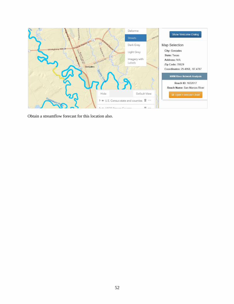
Pan the map to the south east (bottom right) and click on the most downstream stream segment

in the San Marcos Basin (COMID 1632017)

52

Obtain a streamflow forecast for this location also.

53

To be turned in: Screen captures of your National Water Model forecasts of the Blanco River at

Wimberley and the San Marcos River. What is the approximate ratio of the forecast flows at the two

locations? How does this compare to the ratio of their drainage areas? Use the attribute TotDASqKM on

the Flowline feature class to find the drainage areas of these two flowlines.

Ok, you’re done!

_______________________________________________

54

Summary of Items to be Turned in:

1. Make a map of the San Marcos basin with its HUC10 and HUC12 watersheds and

subwatersheds. Use a layout as you learned in exercise 1. How many HUC10 and HUC12 units

exist in the San Marcos Basin? Note that maps that you turn in should be clearly labeled so that

they may be unambiguously interpreted with a title, scale, north arrow and appropriate legend

information.

2. Make a map of the land cover over the San Marcos Basin. Prepare a table that shows the area

(km2) of each of the main land cover classes and the % of the total basin area that each land

cover class represents.

3. Make a map of the San Marcos basin with its labeled rivers. How many Catchments lie within

this basin? What is their average area (Sq. Km)? How many Flowlines lie within this basin?

What is their average length (Km)

4. A layout showing a map and table describing the flow gages in the San Marcos Basin

5. Screen captures of your National Water Model forecasts of the Blanco River at Wimberley and

the San Marcos River. What is the approximate ratio of the forecast flows at the two locations?

How does this compare to the ratio of their drainage areas? Use the attribute TotDASqKM on the

Flowline feature class to find the drainage areas of these two flowlines.