1

Exercise 13: Intermediate Vector Analysis

In this exercise, you will learn to use a variety of vector analysis and geoprocessing methods. You will then use these methods to answer some less guided questions. Individually, these tools can be used to answer simple questions. However, they can be combined to answer more complex questions in a multi-part analysis. GIS professionals commonly use these methods on a daily basis, so they are important to add to your list of skills.

Topics covered in this exercise include:

1. Execute a variety of vector analysis techniques including: dissolve, clip, buffer, intersect, union, spatial joins, and summarization.

2. Use vector analysis tools provided in ArcGIS Pro. 3. Answer spatial analysis questions by combining vector analysis tools.

Step 1. Open a Map Project

First, we need to download and open the Exercise_13.aprx file.

� Download the Exercise_13 lab folder from the class webpage under Education tab on http://www.wvview.org/. All lab material is available under “Labs and Data” tab.

� Click on the “L13 Data” button to download the Exercise_13.zip file. � You will need to extract the compressed files and save it to the

location of your choosing. � Open ArcGIS Pro. This can be done by navigating to All Apps followed

by the ArcGIS Folder. Within the ArcGIS Folder, select ArcGIS Pro. Note that you can also use a Task Bar or Desktop shortcut if they are available on your machine.

� After ArcGIS Pro launches, select “Open another project.”

� Navigate to the directory that houses the material for this course. The project files are in the Exercise_13 folder where it was saved on your local machine.

� Select Exercise_13.aprx. Click OK to open the project. � If necessary, navigate to the WV map.

2

Note: If you’d prefer, you can also just click on the Exercise_13.aprx file within the uncompressed folder directly to launch ArcGIS Pro.

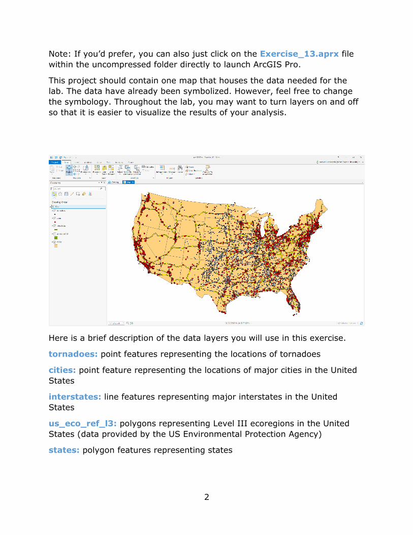
This project should contain one map that houses the data needed for the lab. The data have already been symbolized. However, feel free to change the symbology. Throughout the lab, you may want to turn layers on and off so that it is easier to visualize the results of your analysis.

Here is a brief description of the data layers you will use in this exercise.

tornadoes: point features representing the locations of tornadoes

cities: point feature representing the locations of major cities in the United States

interstates: line features representing major interstates in the United States

us_eco_ref_l3: polygons representing Level III ecoregions in the United States (data provided by the US Environmental Protection Agency)

states: polygon features representing states

3

Step 2. Defining Environment Settings

Since you will perform many spatial analysis operation in this lab, you will start by setting the environment settings. It is generally a good idea to set environment settings any time you will perform spatial analysis operations in a project. Also, this can speed up you processing, as you will not need to set environments for each tool individually. In short, we highly recommend this.

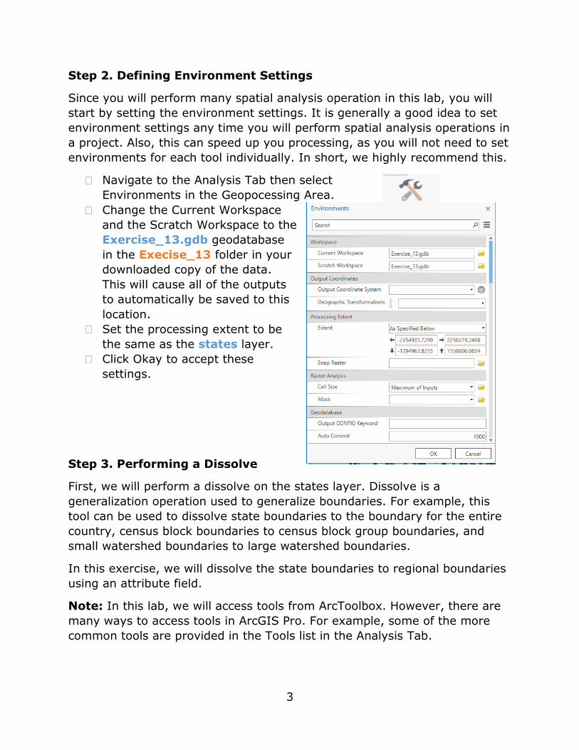
� Navigate to the Analysis Tab then select Environments in the Geopocessing Area.

� Change the Current Workspace and the Scratch Workspace to the Exercise_13.gdb geodatabase in the Execise_13 folder in your downloaded copy of the data. This will cause all of the outputs to automatically be saved to this location.

� Set the processing extent to be the same as the states layer.

� Click Okay to accept these settings.

Step 3. Performing a Dissolve

First, we will perform a dissolve on the states layer. Dissolve is a generalization operation used to generalize boundaries. For example, this tool can be used to dissolve state boundaries to the boundary for the entire country, census block boundaries to census block group boundaries, and small watershed boundaries to large watershed boundaries.

In this exercise, we will dissolve the state boundaries to regional boundaries using an attribute field.

Note: In this lab, we will access tools from ArcToolbox. However, there are many ways to access tools in ArcGIS Pro. For example, some of the more common tools are provided in the Tools list in the Analysis Tab.

4

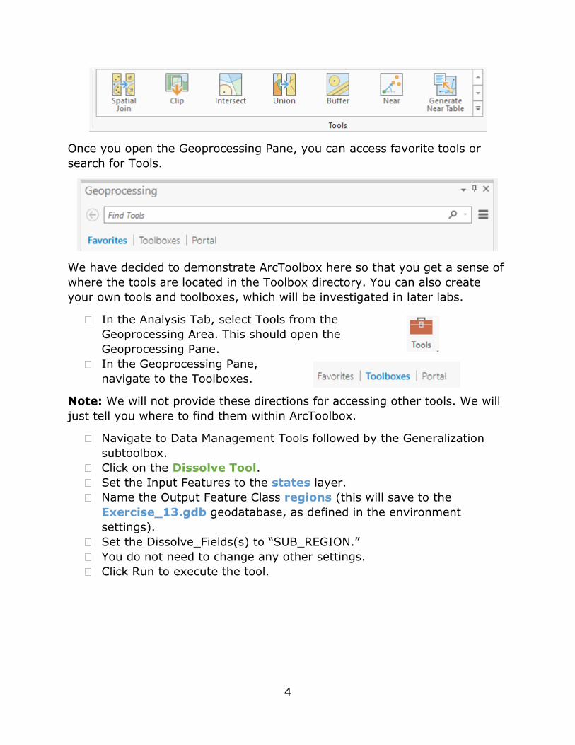
Once you open the Geoprocessing Pane, you can access favorite tools or search for Tools.

We have decided to demonstrate ArcToolbox here so that you get a sense of where the tools are located in the Toolbox directory. You can also create your own tools and toolboxes, which will be investigated in later labs.

� In the Analysis Tab, select Tools from the Geoprocessing Area. This should open the Geoprocessing Pane.

� In the Geoprocessing Pane, navigate to the Toolboxes.

Note: We will not provide these directions for accessing other tools. We will just tell you where to find them within ArcToolbox.

� Navigate to Data Management Tools followed by the Generalization subtoolbox.

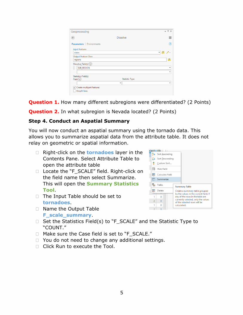
� Click on the Dissolve Tool. � Set the Input Features to the states layer. � Name the Output Feature Class regions (this will save to the

Exercise_13.gdb geodatabase, as defined in the environment settings).

� Set the Dissolve_Fields(s) to “SUB_REGION.” � You do not need to change any other settings. � Click Run to execute the tool.

5

Question 1. How many different subregions were differentiated? (2 Points)

Question 2. In what subregion is Nevada located? (2 Points)

Step 4. Conduct an Aspatial Summary

You will now conduct an aspatial summary using the tornado data. This allows you to summarize aspatial data from the attribute table. It does not relay on geometric or spatial information.

� Right-click on the tornadoes layer in the Contents Pane. Select Attribute Table to open the attribute table

� Locate the “F_SCALE” field. Right-click on the field name then select Summarize. This will open the Summary Statistics Tool.

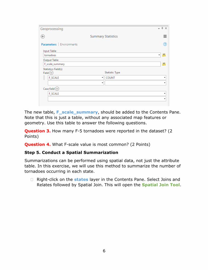
� The Input Table should be set to tornadoes.

� Name the Output Table F_scale_summary.

� Set the Statistics Field(s) to “F_SCALE” and the Statistic Type to “COUNT.”

� Make sure the Case field is set to “F_SCALE.” � You do not need to change any additional settings. � Click Run to execute the Tool.

6

The new table, F_scale_summary, should be added to the Contents Pane. Note that this is just a table, without any associated map features or geometry. Use this table to answer the following questions.

Question 3. How many F-5 tornadoes were reported in the dataset? (2 Points)

Question 4. What F-scale value is most common? (2 Points)

Step 5. Conduct a Spatial Summarization

Summarizations can be performed using spatial data, not just the attribute table. In this exercise, we will use this method to summarize the number of tornadoes occurring in each state.

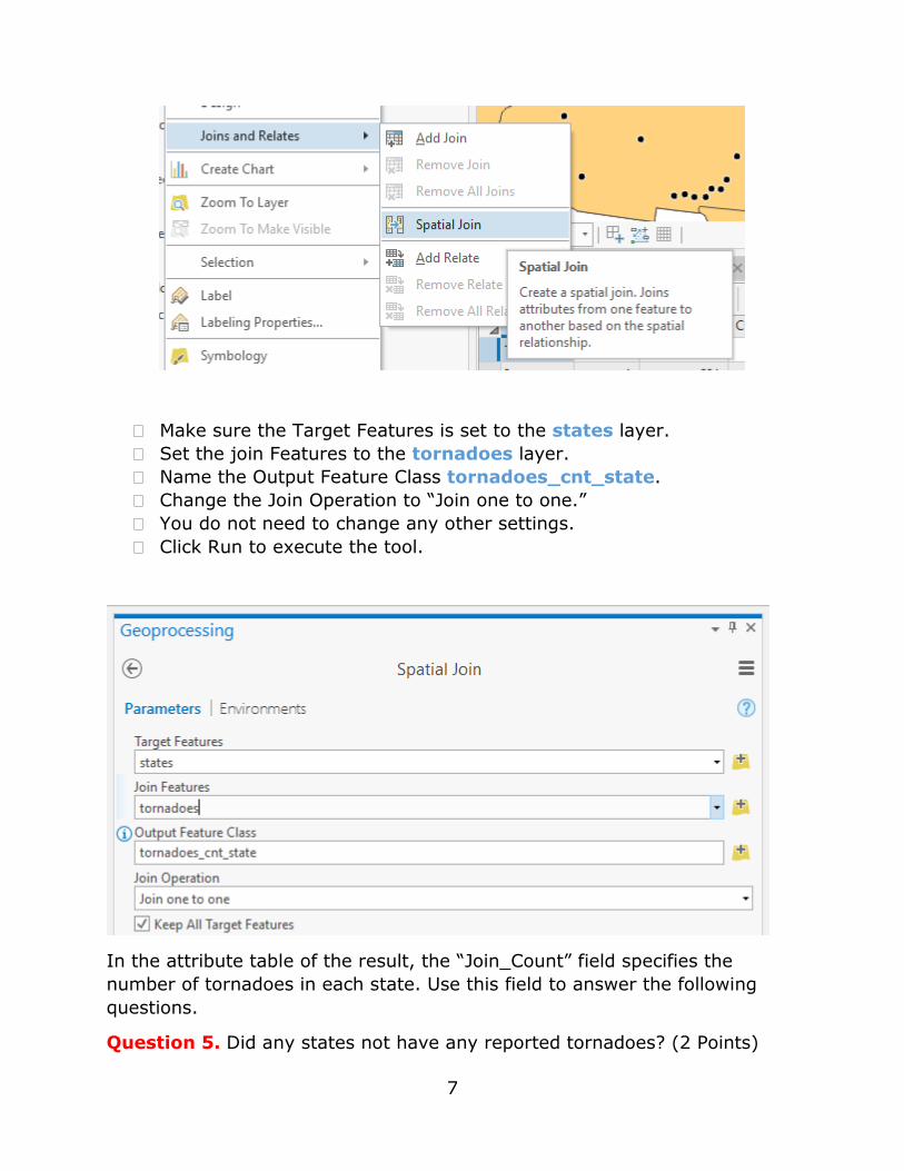
� Right-click on the states layer in the Contents Pane. Select Joins and Relates followed by Spatial Join. This will open the Spatial Join Tool.

7

� Make sure the Target Features is set to the states layer. � Set the join Features to the tornadoes layer. � Name the Output Feature Class tornadoes_cnt_state. � Change the Join Operation to “Join one to one.” � You do not need to change any other settings. � Click Run to execute the tool.

In the attribute table of the result, the “Join_Count” field specifies the number of tornadoes in each state. Use this field to answer the following questions.

Question 5. Did any states not have any reported tornadoes? (2 Points)

8

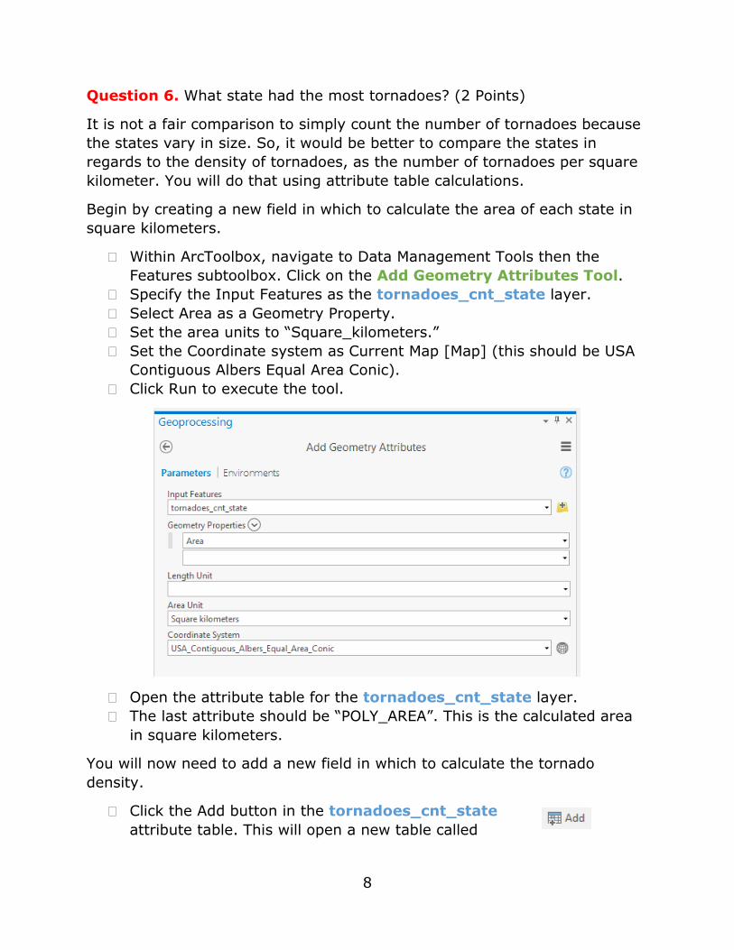
Question 6. What state had the most tornadoes? (2 Points)

It is not a fair comparison to simply count the number of tornadoes because the states vary in size. So, it would be better to compare the states in regards to the density of tornadoes, as the number of tornadoes per square kilometer. You will do that using attribute table calculations.

Begin by creating a new field in which to calculate the area of each state in square kilometers.

� Within ArcToolbox, navigate to Data Management Tools then the Features subtoolbox. Click on the Add Geometry Attributes Tool.

� Specify the Input Features as the tornadoes_cnt_state layer. � Select Area as a Geometry Property. � Set the area units to “Square_kilometers.” � Set the Coordinate system as Current Map [Map] (this should be USA

Contiguous Albers Equal Area Conic). � Click Run to execute the tool.

� Open the attribute table for the tornadoes_cnt_state layer. � The last attribute should be “POLY_AREA”. This is the calculated area

in square kilometers.

You will now need to add a new field in which to calculate the tornado density.

� Click the Add button in the tornadoes_cnt_state attribute table. This will open a new table called

9

Fields: tornadoes_cnt_state. You can add a new field at the bottom of the table.

� Name the new field “tor_den.” You do not need to specify an alias. Set the Data Type to Float.

� In the Fields Tab click Save to add the new field. Note that you can use the New Field button to add fields, as opposed to the method described above.

� Navigate back to the attribute table for tornadoes_cnt_state.

You should have a new column at the end of the table called “tor_den.” However, this field does not yet hold any values and is populated with <Null>. You will now need to calculate the tornado density in this field.

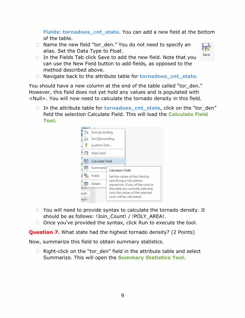
� In the attribute table for tornadoes_cnt_state, click on the “tor_den” field the selection Calculate Field. This will load the Calculate Field Tool.

� You will need to provide syntax to calculate the tornado density. It should be as follows: !Join_Count! / !POLY_AREA!.

� Once you’ve provided the syntax, click Run to execute the tool.

Question 7. What state had the highest tornado density? (2 Points)

Now, summarize this field to obtain summary statistics.

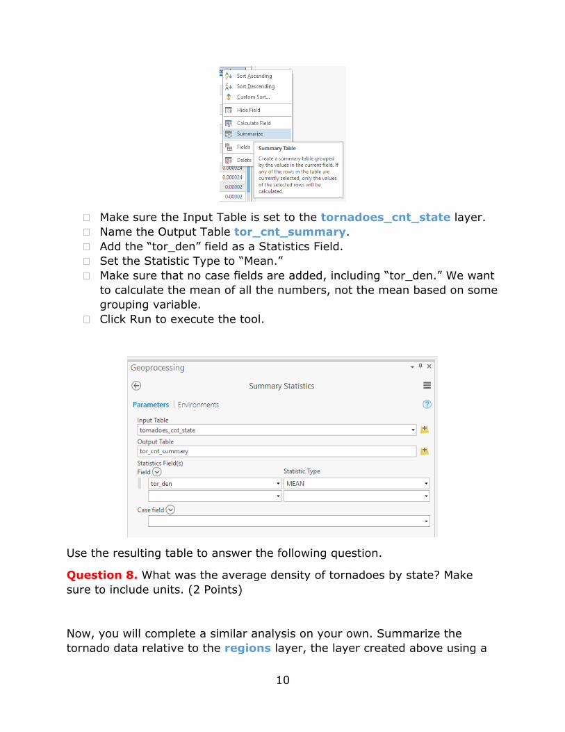
� Right-click on the “tor_den” field in the attribute table and select Summarize. This will open the Summary Statistics Tool.

10

� Make sure the Input Table is set to the tornadoes_cnt_state layer. � Name the Output Table tor_cnt_summary. � Add the “tor_den” field as a Statistics Field. � Set the Statistic Type to “Mean.” � Make sure that no case fields are added, including “tor_den.” We want

to calculate the mean of all the numbers, not the mean based on some grouping variable.

� Click Run to execute the tool.

Use the resulting table to answer the following question.

Question 8. What was the average density of tornadoes by state? Make sure to include units. (2 Points)

Now, you will complete a similar analysis on your own. Summarize the tornado data relative to the regions layer, the layer created above using a

11

dissolve, as opposed to the state layer. You will need to count the number of tornadoes in each region and also calculate the density. Use your results to answer the questions below.

Question 9. Did any subregions not have a tornado? (2 Points)

Question 10. Which subregion had the most tornadoes? (2 Points)

Question 11. Which subregion had the highest density of tornadoes? (2 Points)

Question 12. What was the average number of tornadoes per subregion? (2 Points)

Step 6. Buffer and Clip

You will now make use of the buffer and clip operations to answer a question. Specifically, we would like to find the number of tornadoes that were within 100 miles of the city of Indianapolis, Indiana. Buffer is a form of proximity analysis: it is used to find features or areas that are within a distance of other features. Clip is used to extract features or portions of features that fall within another feature. These are some of the most commonly used vector analysis operations. They have many uses.

First, you will need to extract Indianapolis from the cities layer. You can do so by querying the attribute table.

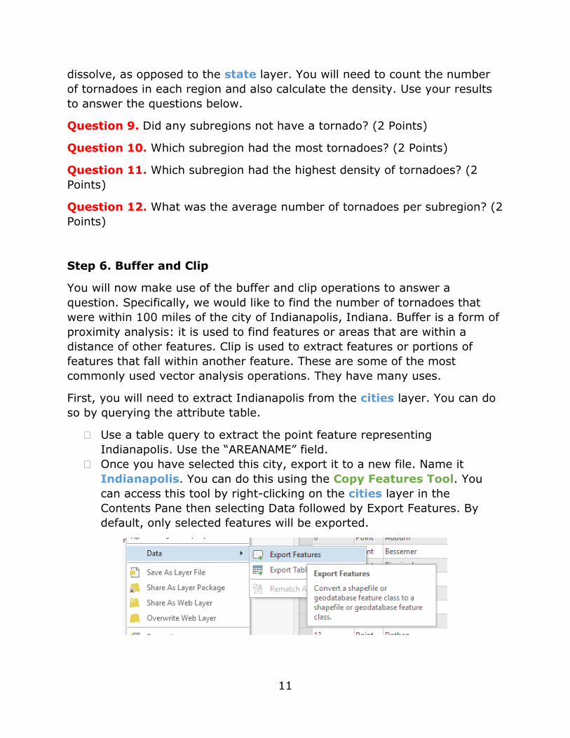
� Use a table query to extract the point feature representing Indianapolis. Use the “AREANAME” field.

� Once you have selected this city, export it to a new file. Name it Indianapolis. You can do this using the Copy Features Tool. You can access this tool by right-clicking on the cities layer in the Contents Pane then selecting Data followed by Export Features. By default, only selected features will be exported.

12

� The exported feature should automatically be added to your map as a new layer.

Note: It is not really necessary to export the feature once it has been selected, as the geoprocessing tools generally will only be conducted for selected features. However, we are demonstrating this step here to show how to export features from a dataset.

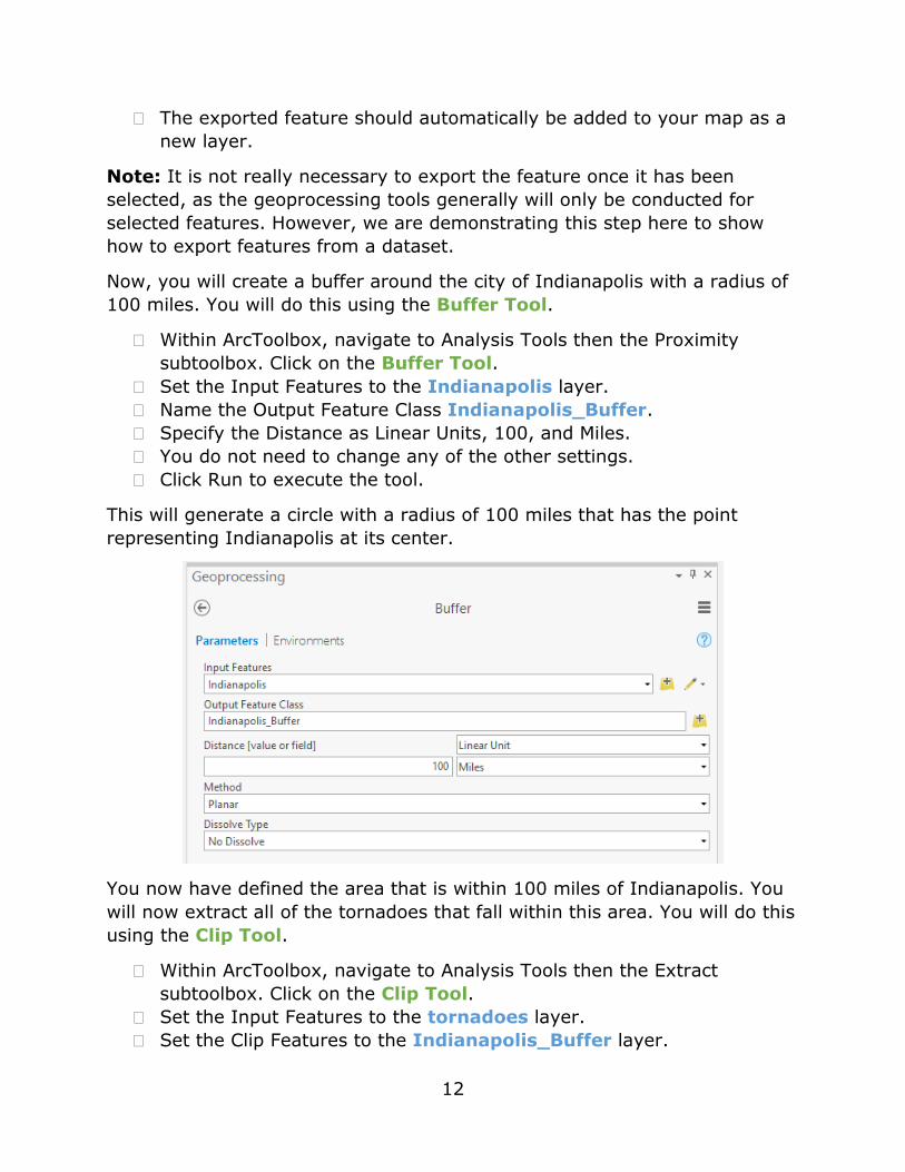
Now, you will create a buffer around the city of Indianapolis with a radius of 100 miles. You will do this using the Buffer Tool.

� Within ArcToolbox, navigate to Analysis Tools then the Proximity subtoolbox. Click on the Buffer Tool.

� Set the Input Features to the Indianapolis layer. � Name the Output Feature Class Indianapolis_Buffer. � Specify the Distance as Linear Units, 100, and Miles. � You do not need to change any of the other settings. � Click Run to execute the tool.

This will generate a circle with a radius of 100 miles that has the point representing Indianapolis at its center.

You now have defined the area that is within 100 miles of Indianapolis. You will now extract all of the tornadoes that fall within this area. You will do this using the Clip Tool.

� Within ArcToolbox, navigate to Analysis Tools then the Extract subtoolbox. Click on the Clip Tool.

� Set the Input Features to the tornadoes layer. � Set the Clip Features to the Indianapolis_Buffer layer.

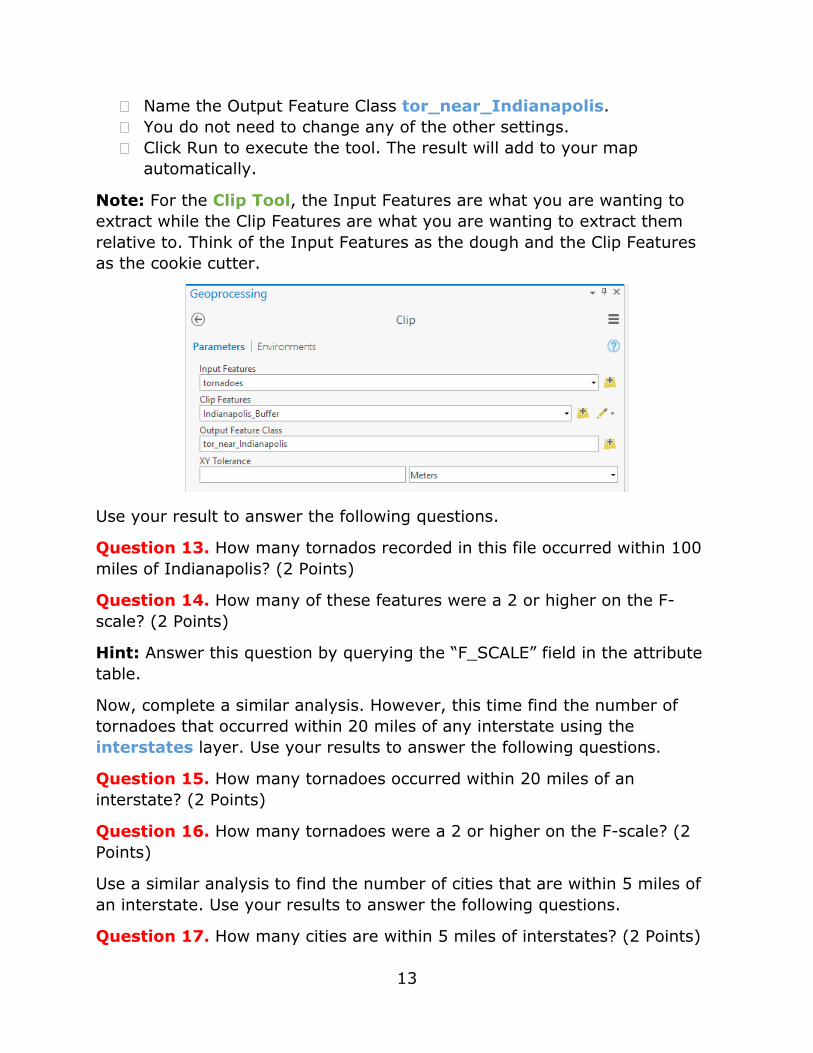
13

� Name the Output Feature Class tor_near_Indianapolis. � You do not need to change any of the other settings. � Click Run to execute the tool. The result will add to your map

automatically.

Note: For the Clip Tool, the Input Features are what you are wanting to extract while the Clip Features are what you are wanting to extract them relative to. Think of the Input Features as the dough and the Clip Features as the cookie cutter.

Use your result to answer the following questions.

Question 13. How many tornados recorded in this file occurred within 100 miles of Indianapolis? (2 Points)

Question 14. How many of these features were a 2 or higher on the F-scale? (2 Points)

Hint: Answer this question by querying the “F_SCALE” field in the attribute table.

Now, complete a similar analysis. However, this time find the number of tornadoes that occurred within 20 miles of any interstate using the interstates layer. Use your results to answer the following questions.

Question 15. How many tornadoes occurred within 20 miles of an interstate? (2 Points)

Question 16. How many tornadoes were a 2 or higher on the F-scale? (2 Points)

Use a similar analysis to find the number of cities that are within 5 miles of an interstate. Use your results to answer the following questions.

Question 17. How many cities are within 5 miles of interstates? (2 Points)

14

Question 18. What percentage is this of all of the cities in the cities layer? (2 Points)

Step 7. Intersection and Union

Two polygon layers have been provided in this lab: states, representing states in the contiguous United States, and us_eco_reg_l3, representing Level III ecoregions in the United States. More information about the ecoregions layer can be found at: https://www.epa.gov/eco-research/level-iii-and-iv-ecoregions-continental-united-states.

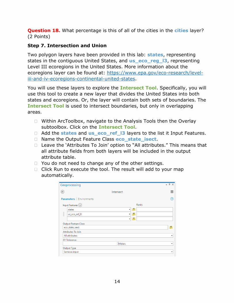
You will use these layers to explore the Intersect Tool. Specifically, you will use this tool to create a new layer that divides the United States into both states and ecoregions. Or, the layer will contain both sets of boundaries. The Intersect Tool is used to intersect boundaries, but only in overlapping areas.

� Within ArcToolbox, navigate to the Analysis Tools then the Overlay subtoolbox. Click on the Intersect Tool.

� Add the states and us_eco_ref_l3 layers to the list it Input Features. � Name the Output Feature Class eco_state_isect. � Leave the ‘Attributes To Join’ option to “All attributes.” This means that

all attribute fields from both layers will be included in the output attribute table.

� You do not need to change any of the other settings. � Click Run to execute the tool. The result will add to your map

automatically.

15

Note: When geoprocessing operations are performed that change the geometry of the resulting features, geometric fields in the attribute table are not automatically updated. For example, in this analysis there is a field in the states layer called “AREA” that give the area for each state. This area will not be updated to show the correct area of the resulting features once the states have been split along the ecoregion boundaries. So, be cautious when using geometric fields, as they can be incorrect as a result of the geoprocessing operations performed. You can always calculate new geometric fields.

Use the results of this analysis to address the following questions.

Question 19. How many features were created as a result of the intersection? (2 Points)

Question 20. How many features are within Texas? (2 Points)

Hint: You can find this answer by querying the attribute table of the output and using the “STATE_NAME” field.

Question 21. How many features are recorded in the Middle Rockies Level III region? (2 Points)

Hint: Use the “US_L3NAME” field.

Now, you will find the state that has the most unique Level III ecoregions within it. Before you undertake this analysis, make sure to clear your selections. First, you will use the Dissolve Tool to combine all features that are in the same state and are the same Level III ecoregion.

� Navigate to Data Management Tools followed by the Generalization subtoolbox.

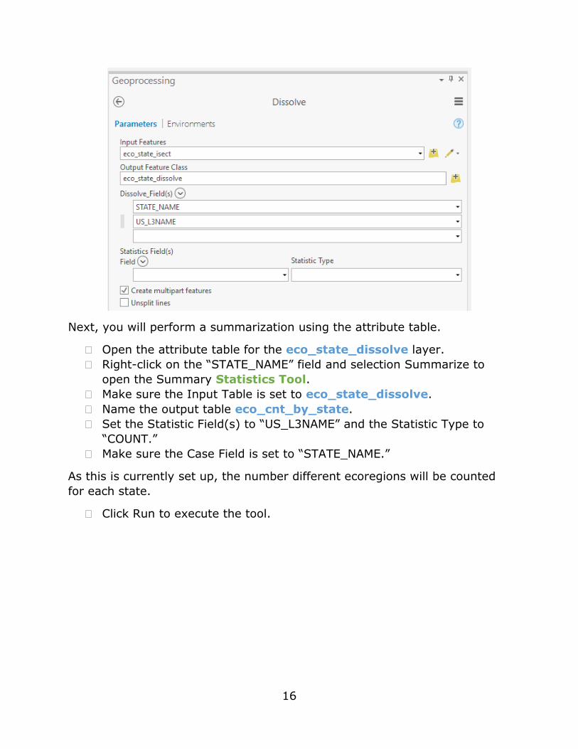
� Click on the Dissolve Tool. � Set the Input Features to the eco_state_isect layer. � Name the Output Feature Class eco_state_dissolve. � Set the Dissolve_Fields(s) to “STATE_NAME” and “US_L3NAME.” � You do not need to change any other settings. � Click Run to execute the tool.

16

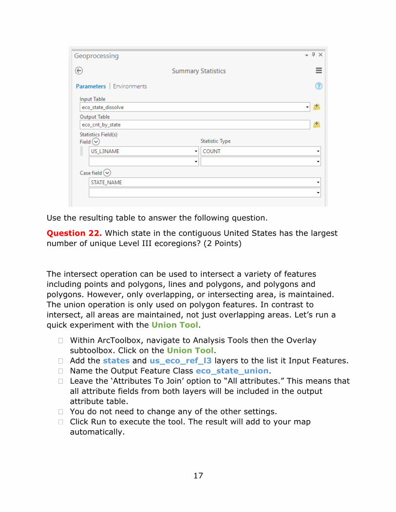
Next, you will perform a summarization using the attribute table.

� Open the attribute table for the eco_state_dissolve layer. � Right-click on the “STATE_NAME” field and selection Summarize to

open the Summary Statistics Tool. � Make sure the Input Table is set to eco_state_dissolve. � Name the output table eco_cnt_by_state. � Set the Statistic Field(s) to “US_L3NAME” and the Statistic Type to

“COUNT.” � Make sure the Case Field is set to “STATE_NAME.”

As this is currently set up, the number different ecoregions will be counted for each state.

� Click Run to execute the tool.

17

Use the resulting table to answer the following question.

Question 22. Which state in the contiguous United States has the largest number of unique Level III ecoregions? (2 Points)

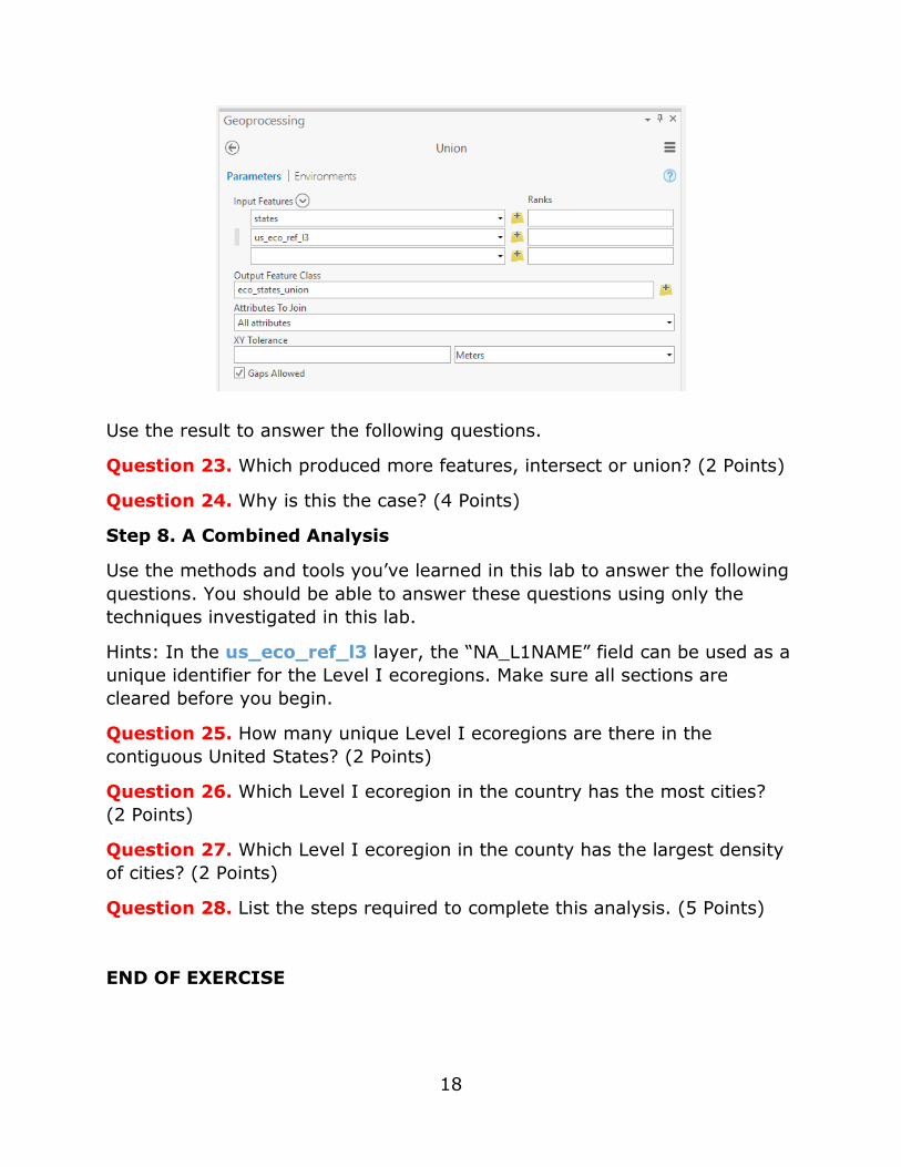
The intersect operation can be used to intersect a variety of features including points and polygons, lines and polygons, and polygons and polygons. However, only overlapping, or intersecting area, is maintained. The union operation is only used on polygon features. In contrast to intersect, all areas are maintained, not just overlapping areas. Let’s run a quick experiment with the Union Tool.

� Within ArcToolbox, navigate to Analysis Tools then the Overlay subtoolbox. Click on the Union Tool.

� Add the states and us_eco_ref_l3 layers to the list it Input Features. � Name the Output Feature Class eco_state_union. � Leave the ‘Attributes To Join’ option to “All attributes.” This means that

all attribute fields from both layers will be included in the output attribute table.

� You do not need to change any of the other settings. � Click Run to execute the tool. The result will add to your map

automatically.

18

Use the result to answer the following questions.

Question 23. Which produced more features, intersect or union? (2 Points)

Question 24. Why is this the case? (4 Points)

Step 8. A Combined Analysis

Use the methods and tools you’ve learned in this lab to answer the following questions. You should be able to answer these questions using only the techniques investigated in this lab.

Hints: In the us_eco_ref_l3 layer, the “NA_L1NAME” field can be used as a unique identifier for the Level I ecoregions. Make sure all sections are cleared before you begin.

Question 25. How many unique Level I ecoregions are there in the contiguous United States? (2 Points)

Question 26. Which Level I ecoregion in the country has the most cities? (2 Points)

Question 27. Which Level I ecoregion in the county has the largest density of cities? (2 Points)

Question 28. List the steps required to complete this analysis. (5 Points)

END OF EXERCISE