Executive Summary - Morgan State University · Web viewThe first questionnaire was focused on...

State Highway AdministrationResearch Report

Quantifying Travel Time Reliability Perception and Developing Disaggregate Behavior Models under Information Provision Using Integrated

Driving/Traffic Simulation

Mansoureh JeihaniZohreh Rashidi Moghaddam

Farzad Moazzami

Project Number: SHA/MSU4

FINAL REPORT

August 2016

Larry Hogen, Governor

Boyd Rutherford, Lt. Governor

Beverley K. Swaim-Staley, Secretary

Darrell B. Mobley, Acting Administrator

The contents of this report reflect the views of the authors who are responsible for the facts and the accuracy of the data presented herein. The contents do not necessarily reflect the official views or policies of the Maryland State Highway Administration. This document is disseminated under the sponsorship of the U.S. Department of Transportation, University Transportation Centers Program, in the interest of information exchange. The U.S. government assumes no liability for the contents or use thereof. This report does not constitute a standard, specification or regulation.

ii

Form DOT F 1700.7 (8-72) Reproduction of form and completed page is authorized.

iii

Technical Report Documentation Page1. Report No. 2. Government Accession No. 3. Recipient's Catalog No.

4. Title and SubtitleQuantifying Travel Time Reliability Perception and Developing Disaggregate Behavior Models under Information Provision Using Integrated Driving/Traffic Simulation

5. Report DateAugust 2016

6. Performing Organization Code

7. Author/s Mansoureh Jeihani, Zohreh Rashidi Moghaddam

8. Performing Organization Report No.

9. Performing Organization Name and AddressMorgan State University1700 E. Cold Spring LaneBaltimore, MD 21251

10. Work Unit No. (TRAIS)

12. Sponsoring Organization Name and AddressOffice of Policy and ResearchMaryland State Highway Administration707 N. Calvert St.Baltimore, MD 21202

National Transportation CenterMorgan State University1700 E. Cold Spring LaneBaltimore, MD 21251

11. Contract or Grant No.SHA/MSU4

13. Type of Report and Period CoveredFinal Report

14. Sponsoring Agency Code

15. Supplementary Notes

16. AbstractThis study investigates travelers’ perception of and response to travel time information and its reliability, in terms of their route choice behavior elicited through a driving simulator and a stated preference (SP) survey. In the driving simulator-based experiments, a 220 mi2 network in Maryland is developed, and different scenarios of traffic and driving conditions, information provision, and reliability levels are considered. The travel time information is provided using a variable message sign (VMS). There are three major routes between the origin and destination, one of which is a toll road. 216 experiments are conducted using a sample of 65 participants from diverse socioeconomic backgrounds. Binary and multinomial logistic regression models are used to analyze the collected data. The results illustrate that trip purpose, travel time reliability, congestion level, and income are important determinants of drivers’ route choice and compliance behaviors. The route choice behavior revealed through the driving simulator is shown to be significantly different from that stated in the survey questionnaire.

17. Key Words: Variable message sign; Compliance behavior; Route choice behavior; Logistic regression; Driving simulator

18. Distribution Statement: No restrictionsThis document is available from the Research Division upon request.

19. Security Classification (of this report)None

20. Security Classification (of this page)None

21. No. of Pages 67

22. Price

Table of Contents

Executive Summary....................................................................................................................1

Introduction.................................................................................................................................2

Literature Review........................................................................................................................3

Data Collection Methods........................................................................................................4

Travel Time and Travel Time Reliability...............................................................................5

Methodology...............................................................................................................................8

Driving Simulator...................................................................................................................8

Network Design......................................................................................................................9

Scenario Design....................................................................................................................12

Survey Questionnaires..........................................................................................................15

Driving session’s rules..........................................................................................................15

Recruitment Process..............................................................................................................16

Participants’ characteristics..................................................................................................17

Research Findings and Discussion............................................................................................21

Attitude Analysis..................................................................................................................21

Stated Preference Analysis...................................................................................................25

Revealed Choice Analysis....................................................................................................27

Compliance Model................................................................................................................32

Route Choice Model.............................................................................................................33

Conclusion................................................................................................................................35

Works Cited..............................................................................................................................37

Appendix A: Survey Questionnaire 1..........................................................................................I

Appendix B: Survey Questionnaire 2.......................................................................................IV

Appendix C: Survey Questionnaire 3.................................................................................XVIII

Appendix D: Consent Form...................................................................................................XXI

i

List of Figures

Figure 1. Interaction of a transportation system’s components with travel time reliability information......................................................................................................................................3

Figure 2- The driving simulator owned by morgan state university...........................................9

Figure 3- A snapshot of developed network in driving simulator..............................................9

Figure 4- The developed network in the driving simulator......................................................10

Figure 5- The study area and main alternatives........................................................................11

Figure 6- A sample of the three phases of traffic genetors in the driving simulator................12

Figure 7- Participants' view of VMS in three scenarios...........................................................14

Figure 8- The process of subject recruitment...........................................................................16

Figure 9- Distribution of participants’ gender..........................................................................18

Figure 10- Distribution of participants’ age group...................................................................19

Figure 11- Distribution of participants’ education level...........................................................19

Figure 12- Distribution of participants’ work status.................................................................19

Figure 13- Distribution of participants’ household size...........................................................20

Figure 14- Distribution of participants’ annual income............................................................20

Figure 15- Distribution of number of cars in participants’ household......................................20

Figure 16- Distribution of participants’ annual mileage...........................................................21

Figure 17- Participants' level of attention to a VMS based on their exposure to VMS............22

Figure 18- Participants’ level of attention to VMS in usual trips.............................................23

Figure 19- Participants’ level of attention to VMS in work trips.............................................23

Figure 20- VMS attention level based on participants’ attitude toward VMS.........................24

Figure 21- GPS usage among participants................................................................................24

Figure 22- Traffic advisory radio usage among participants....................................................25

Figure 23- Participants' familiarity with the study area............................................................25

Figure 24- The stated route choice of participants who were familiar with the study area......26

Figure 25- The average of stated travel time anticipation for each route.................................26

Figure 26- Participants’ preference for travel time information provision format on VMS....27

ii

Figure 27- Comparison of PTT versus ATT for the simulation experiment............................30

Figure 28- PTT versus ATT for each option in each non-work scenario.................................30

Figure 29- Participants’ belief toward travel time reliability in the driving simulator.............31

Figure 30- The stated route choice of participants after the driving simulation experiment....32

iii

List of Tables

Table 1- Discriprition of designed scenarios............................................................................13

Table 2- Descriptive statistics of socio-economic data.............................................................17

Table 3- Compliance rate analysis for simulation experiments................................................28

Table 4- Comparison of stated route in survey versus revealed choice in simulator...............29

Table 5- Comprison of stated versusrevealed choice for the ICC toll road..............................29

Table 6- Correlation of independent variables and compliance variable.................................33

Table 7- Compliance model results..........................................................................................33

Table 8- Route choice model result..........................................................................................34

iv

ACKNOWLEDGEMENTS

The authors would like to thank the Maryland State Highway Administration for its funding support and input throughout the study.

Shive Narooeinezhad played an important role in network design and Samira Ahangari, Alasan Jajru and Kiante Bush assisted in data collection and their work is appreciated.

v

Executive Summary

This study investigates travelers’ perception of and response to travel time information and its reliability, in terms of their route choice behavior elicited through a driving simulator and a stated preference (SP) survey. In the driving simulator-based experiments, a 220 mi2 network in Maryland is developed, and different scenarios of traffic and driving conditions, information provision, and reliability levels are considered. The travel time information is provided using a variable message sign (VMS). There are three major routes between the origin and destination, one of which is a toll road. 216 experiments are conducted using a sample of 65 participants from diverse socioeconomic backgrounds. Binary and multinomial logistic regression models are used to analyze the collected data. The results illustrate that trip purpose, travel time reliability, congestion level, and income are important determinants of drivers’ route choice and compliance behaviors. The route choice behavior revealed through the driving simulator is shown to be significantly different from that stated in the survey questionnaire.

1

Introduction

Transportation plays a key role in today’s world. Modern lives are affected by it, starting in the morning, when people commute to work by car or public transportation, through the evening, when they get back home. However, transportation does not just affect our lives by providing a means of commuting to work; it’s deeply rooted in every aspect of our daily lives in such a way that modern life seems to be impossible without it. People need to get to work on time, catch flights, attend meetings, and arrive at their doctor’s office before their appointment – for all of these events, the key factor is time. They need to know how much time they should allow for transportation to be on time. In these cases, travel time reliability has a major role to play.

Travel time reliability usually refers to the variation in travel time for the same trip from day to day and at different hours of a day (Strategic Highway Research Program (SHRP2), 2013). The larger the variability in travel time, the more unreliable the travel time is. In a reliable route, travel time would be predictable all the time. However, fluctuation, incidents, inclement weather conditions, poor traffic signal adjustments and many unpredictable circumstances may happen, which result in different travel times for the same origin and destination (List, Williams, &Rouphail, 2014). It should be noted that a reliable route in terms of travel time does not necessarily mean traveling at the speed limit. However, it provides users with a predictable travel time, helping them make better route decisions accordingly.

Travel time reliability is crucial from two points of view: passenger and freight transportation, as well as transportation organizations and traffic managers. With travel time reliability, passengers can make better use of their time on a daily basis and reduce their trip costs by making better decisions prior to their trips or even en-route. Reliable transportation systems provide more predictable travel times, which allow people to have an improved schedule. Travel time reliability is also important for shipping systems. One of the most important parts of every industry is inventory management. Utilizing “Just-in-Time” deliveries lowers total cost by better managing inventory and storage. Every company and industry needs their shipment right before, not after, it is needed. In this case, a reliable transportation system can increase the quality of service of a shipping system and also reduce delivery costs for shippers. In addition, as mentioned before, travel time reliability information is an essential piece of information for transportation engineers and traffic managers, enabling them to better control the regional traffic(Lin, Zito, & Taylor, 2005). By using this information and improving the studied region, they can offer better and more stable quality of service, which results in more traffic safety. Moreover, in a reliable transportation system, fewer vehicles are accelerating and decelerating, reducing fuel consumption and emission of greenhouse gases (Recker, et al., 2004).

2

There are seven sources of congestion that cause unreliable travel time in a transportation network: demand fluctuation, physical bottlenecks, special events, incidents, weather, traffic control devices and work zones. Short-term and long-term approaches can be used to respond to these sources of congestion, and to mitigate travel time uncertainty. Addition and expansion of highways represent long-term solutions. Providing travel-related information to drivers and pricing mechanisms are examples of short-term approaches to influence travelers to make better route decisions (Strategic Highway Research Program (SHRP2), 2013). This information can be conveyed to drivers through radio stations or Variable Message Signs (VMS). The interaction of a transportation system’s components with travel time reliability information is shown in Figure1. As shown, motorists including passengers and freight shippers use the road network and make route decisions. Meanwhile, one or more congestion sources may lead to some routes becoming unreliable, and cause drivers to change routes. Using data collection methods such as license plate recognition, inductive loop detectors and Global Positioning System (GPS), users’ travel times are collected and analyzed to measure travel time reliability. This information can be used by traffic managers to improve network performance or provided to motorists to help them make better travel decisions.

Figure 1. Interaction of a transportation system’s components with travel time reliability information

3

Literature Review

There are several approaches in literature that use different methods for collecting required data and analyzing them to measure the performance of the route of interest. In this section, these methods are discussed separately for data collection and travel time reliability measures.

Data Collection Methods

Calculating all travel time reliability measures is based on a database that contains the required information for the route and trip of interest. Computing statistical measures can be provided by fitting statistical models on this data. Data collection methods can be categorized in two types: site-based and vehicle-based groups. Loop detectors, radars and video processing techniques are examples of site-based methods, while using probe vehicles and GPS are in the vehicle-based group. The site-based methods are explained below:

Radio-Frequency Identification (RFID) is a good use of the wireless transferring of

data between a transmitter and responder. Transponders, the short form of transmitter-

responder, are a combination of tags located in vehicles and receivers in specified

locations such as toll station. EZ-Pass on the East Coast and Fastrak in California are

well-known samples of this technology. Receivers in toll stations on highways, in

addition to the automatic collection of the toll, are able to record the time and the

vehicles’ speed. Traffic volume and speed can be obtained from this record. The

infrastructure and installment cost of this system is high and it is not economically

feasible to use this system for arbitrary locations in the network to calculate travel

time between them.

License Plate Recognition (LPR) uses video/image processing techniques on recorded

videos/images from cameras installed along the roadways to read vehicles’ plates

numbers. An identified vehicle’s speed passing two cameras can be calculated since

cameras also record the exact time of passing. (Bertini et al., 2005) Infrastructure cost

can be a limitation in this approach as in the previous one.

Inductive loop detectors, installed in the pavements or shoulder of highways, utilize

electromagnetic attributes to detect a vehicle passing or arriving at a certain location.

The detector’s electronic unit circulates energy into the wire loops and makes

inductance with specified frequency. A vehicle passing this detector reduces its

inductance and changes the behavior of the inductive loop. Thus, required information

4

such as the number of vehicles passing in a period of time, their speed, traffic volume

and lane occupancy can be recorded by these detectors.

Although real-time travel time information can be collected from sources explained above, the needed equipment is expensive to initialize and maintain. As mentioned before, the other method to collect data is using equipped vehicles traveling in the route of interest, known as probe or floating vehicles (Schwarzenegger, Bonner, Iwasaki, & Copp, 2008). This method is explained below:

Global Positioning System (GPS), mainly used for navigation, is a system that can

provide information about position, velocity and direction of the vehicles with GPS

devices. GPS devices can be found in the market easily at a reasonable price, and their

increasing use is making this system a significant source of accurate data. In addition,

since the obtained data is recorded, both real-time and historical analysis of traffic and

travel time reliability is available (Obuhuma & Moturi, 2012). In this method, transit

buses, taxis, FedEx/UPS trucks and all dedicated vehicles can be used as the probe

vehicles and provide a massive database to analyze (Bertini & Tantiyanugulchai,

2003). Moreover, the increasing use of cellphones equipped with the feature of exact

locating can also make these devices useful as a source of traffic data (Herrera, et al.,

2010).

A literature review on travel time reliability is also provided in next section.

Travel Time and Travel Time Reliability

While travel time is an effective factor for travelers to make a decision about their route, it can vary from day to day or at different hours of the day. Travel time can increase during peak hours of a day or when congestion and incidents result in delays. Travelers are usually not tolerant of unexpected delays. Simple average travel time is not sufficient to report to them as a measure of service since they usually remember their bad experiences of being stuck in heavy traffic, even if only a few times, rather than their normal trips without heavy traffic. Therefore, recent studies suggest models that use both travel time and travel time reliability for a specified route. Travel time reliability, more accurately, relates to travel time variability and has a key role in the quality of service of a transportation system. The less variability and more dependability in travel times from day-to-day, the more reliable is the studied route (FHWA, Travel TimeReliability: Making It There On Time, All The Time, 2006).

5

Small et al. (Small, Noland, & Chu, 1999) showed that congestion not only increases the travel time average but also its standard deviation; in other words, longer and more unpredictable trips. To provide the travel time reliability values for users, they collected data based on survey instruments for two groups: passengers and freight shippers. They showed that passengers have different views on the importance of travel time reliability for travel. For example, travelers commuting to work and business value travel time reliability more than people traveling for non-work purposes. For freight shippers, since the loss cost is more crucial based on expected delivery time and the nature of their shipment, travel time reliability is even more important.

Chen et al. (Chen, Skabardonis, & Varaiya, 2003) analyzed data from a corridor in Los Angeles to show that the travel time reliability can be used as a good measure of freeway performance. By using data from detectors at specific locations on freeways to estimate speed, they showed that the travel time mean and its standard deviation are highly correlated. As the average travel time increases, the standard deviation also increases, implying more uncertainty under congestion. Hence, travel time reliability and its predictability are indicators of how well a freeway serves travelers.

Liu et al. (2004) (Liu, Recker, & Chen, 2004) proposed a method to show the importance of travel time reliability on travelers’ route choice. Using a genetic algorithm on data obtained from Revealed Preference (RP) and Stated Preference (SP) surveys, they concluded that the value of travel time was $12.81 per hour while the value of reliability was $20.63 per hour. This shows how travel time reliability is significant for travelers’ route choices.

The Federal Highway Administration (2005) (FHWA, Traffic Congestion and Reliability:,2005) defined some measures, as shown below, to report travel time reliability in a manner suitable and understandable for both technical transportation audiences and non-technical travelers.

Travel window is the combination of average travel time and its standard deviation.

Travel window is usually shown as:

Travel Window=AverageTravel Time± Standard Deviation

Percent Variation which is shown in below equation.

Percent Variation= Standard DeviationAverageTravel Time

×100

90 th or 95 th percentile travel times is one of the simplest measures of travel time reliability

which shows that 90 or 95 percent of the time, travel time is equal or less than this

measure respectively. Since this measure is more likely to be understood by commuters, it

is suited for reporting needed information to travelers. The 95th percentile is referred to as

6

Planning time (PT) and represents the total time that should be planned before starting a

trip.

The buffer time (BT) states the needed extra time to ensure travelers reach their

destination on time. It can be simply defined as the difference between the Planning time

and the average travel time.

The buffer time index (BTI) is reported as a percentage and can be computed as below:

Buffer time index=95th percentile travel time−average travel timeaveragetravel time

The planning time index (PTI) is also the ratio of the planning time over the free-flow

travel time. This measure can be useful in reporting “near-worst case” travel time.

The steps of measuring travel time reliability were introduced as defining travel modes, routes, trips, days and times of interest, collecting and processing required data and calculating reliability measures to report.

Van Lint et al. (2005) (van Lint & van Zuylen, 2005), introduced two metrics to model travel time reliability. They analyzed the data from the Rotterdam Beltway and captured its relation with travel time distribution width and skewness. As was expected, large values for distribution width present more uncertainty and more unreliability due to congestion as a result. The metric skewness is also related to congestion, interestingly. It is approximately 1, small (<<1) and large (>>1) in free-flowing traffic, seriously congested conditions and during setting in/dissolving congestion respectively.

Emam et al. (2006) (Emam & Al-Deek, 2006), tested four distributions – Weibull, exponential, lognormal and normal – on the same data from evening-peak time to see which one fits better on the data. To evaluate these distributions, AD test and error percentages were performed. They found that the lognormal distribution fits the best on travel time reliability distribution.

Ravi Sekhar et al. (Ravi Sekhar, Madhu, Kanagadurai, & Gangopadhyay, 2013) combined the methods of vehicle license plate recognition and traffic volume data obtained from detectors and probe vehicles. They developed a traffic simulation model and analyzed travel time reliability measures using this model. They concluded that among the travel time reliability measures, Buffer Time and Buffer Time Index are more suitable for business-related users while Planning Time and Planning Time Index are useful for normal traffic users.

Quantifying driver perception of travel time information requires a realistic understanding of driver behavioral and cognitive attitudes. This represents a key gap in the current literature (Sharma, Hsu, Soon, & Peeta, 2012). This is particularly important for interpreting driver

7

perceptions of travel time reliability because there are multiple characteristics of information that can affect driver perception and response. These include the issues of multi-tasking, information from multiple sources, and the usefulness of the information available to the particular traveler.

Ardeshiri et al. (Ardeshiri, Jeihani, & Peeta, 2015) utilized driving simulator and stated preference survey methods to analyze drivers’ route choice behavior under real-time route guidance through VMSs. The concluded that past exposure to VMS, travel time savings, VMS information reliability, and learning from past experience affect route choice behavior.

To quantify the impacts of travel time reliability perception and traveler behavior under variability in traffic conditions, this study seek to link information provision and travel time reliability perception to travelers’ route choice behavior using a real-world network in Maryland where one of the routes is a toll road.

This is particularly important for interpreting driver perceptions of travel time reliability because there are multiple characteristics of information that can affect driver perception and response. These include the issues of multi-tasking, information from multiple sources, and the usefulness of the information available to the particular traveler.

Methodology

Driving Simulator

This study utilizes a driving simulator with VR-Design Studio software (Former name: UC-win/Road) from FORUM8 Co. Ltd (Forum8, n.d.) owned by Morgan State University (MSU). This computer-based simulator enables researchers to create a network very similar to the real network and collect details of driver’s route choice in addition to several other useful parameters including but not limited to geographic positions, speed, distance traveled, offset from road’s shoulder, acceleration, brake and yaw/pitch/roll angle. The hardware, as shown in Figure 2 is very similar to a real car and consists of the driver seat, cockpit, steering wheel, acceleration and brake pedals, ignition key, gear stick, flash lights and three surrounding monitors to provide a 3D view. The VR-Design Studio software is a virtual reality system, capable of creating and editing network elements including road alignments, intersection design, traffic signals, cross sections, roadside signs, terrain setup and traffic generation. The software provides the real-time presentation of traffic flow, weather conditions, spatial environment and static objects. A snapshot of the built environment in this study is shown in Figure 3. Since this simulator enables drivers to drive anywhere in a semi-real network and choose their own way from origin to destination, it can be utilized in route choice behavior and road safety studies.

8

In this study, human subjects (briefly called subjects or participants) were asked to start a journey from a fixed origin to a known destination in a predefined traffic condition. The simulator recorded the chosen route in addition to many other useful parameters such as spot speed, lane changing, crashes and actual travel time.

Figure 2- The driving simulator owned by morgan state university

Figure 3- A snapshot of developed network in driving simulator

Network Design

A 20 mi×11 mi (220 mi2) network covering from southwest of Baltimore to downtown Rockville was created in the driving simulator software. Using online mapping system available in Google Maps, all roadway signs, VMS, trees and some buildings were created in the simulated network in accordance with the real world. The road network and surrounding environment were designed as close as possible to the actual environment to ensure that subjects experience similar conditions and have realistic reactions accordingly. Figure 4 shows the study area including the

9

roadways, origin, destination and the position of VMS. The journey for subjects starts on I-95 and ends in Rockville at the intersection of MD-586 and MD-28 (both marked with asterisk). As shown on the map, there are three main alternatives to reach the destination including MD-198, MD-200 and I-495 which are 16, 17 and 23 miles respectively.

The first alternative is route MD-198 continuing to MD-28. MD-198 is a four to six lane divided highway in Maryland. Speed limit of 35-40 mph and numerous intersections and junctions make this route a local road. Moreover, it has a two-lane section before MD-28 with speed limit of 35 mph which increases travel time significantly compared to the other options. In real life, it usually takes 30 to 35 minutes during off-peak hours and 35 to 60 minutes during peak hours to get to the destination using this route.

MD-200, known as Intercounty Connector (ICC), is a six-lane toll freeway which connects I-370 in eastern Montgomery County to US 1 in northwestern Prince George’s County. Currently, the toll for this route is $0.22 per mile in peak hours, $0.17 per mile in off-peak hours and $.07 per mile overnight. Travel time for this option is 22 minutes in off-peak hours and 24-40 minutes in peak hours.

I-495, known as Capital Beltway, is an interstate highway surrounding Washington DC. This highway has four lanes in each direction in the study area with speed limit of 55 mph. The journey from this alternative takes typically 28 minutes in off-peak hours and between 40 minutes to more than 1 hour in peak hours. This wide range shows how congested and unreliable this route can be during peak hours. Figure 5 shows these alternatives on the map more clearly.

10

Figure 4- The developed network in the driving simulator

Figure 5- The study area and main alternatives

The VMS is located on I-95, one mile before the first decision point, MD-198 off-ramp. The VMS presents estimated travel time for each alternative. To ensure that the resulting travel times in each scenario is the same as average actual travel time, the network was driven numerous times by the research team. High congestion level in this network was assured mainly by

11

growing traffic volume and decreasing traffic speed accordingly. In order to have a realistic traffic pattern in the network and prevent crashing of the network due to the limitations of the software, traffic is generated only in the surrounding area of the participant’s vehicle. This is done by using the cycle feature of VR-Design Studio which allows having various phases in a cycle of a traffic generator for each road segment. Three phases are considered for each traffic generator, namely idle1, busy and idle 2. The generator starts with the first idle phase and produces only one vehicle per lane per hour; then it increases the generating rate to the assigned rate in busy phase and reduces it again to one vehicle/lane/hour for the second idle phase. To determine the possible location of participant’s vehicle and the duration of each phase accordingly, a minimum and maximum speed is considered for the vehicle. Based on these speeds, the latest and earliest time that participant’s vehicle reaches the generating points are calculated. Then the phases’ duration of each traffic generator is computed to have network vehicles with the assigned speed before the participant’s vehicle is reached to the generator. Figure 6 shows all traffic generators in the network in one traffic condition and their phases in seconds.

I-95MD-198Road 39MD-200

MD-97I-495

MD-355MD-28

I-270MD-586MD-193MD-185

0 200 400 600 800 1000 1200 1400 1600 1800 2000

47058126

772349

9361402

10321301

472602

80288

936318

438392

474495

549594

586625

18301668

9621512

7461216

54760

37561

898729

Idle 1 Busy Idle 2

Time (seconds)

Tra

ffic

Gen

erat

ors

Figure 6- A sample of the three phases of traffic genetors in the driving simulator

Scenario Design

Seven scenarios were developed in this study to cover different traffic conditions including AM-peak and off-peak, trip purposes namely work and non-work trips and travel time reliabilities. Different levels of reliability in scenarios are defined by exact time, short range and

12

large range for high, medium and low reliability respectively. In the first scenario, the VMS is off and no information about routes is provided to study the participants’ route choice behavior in the absence of travel time information. This scenario is considered to be the base scenario. The second scenario has the same traffic condition as scenario 1, except the VMS provides travel time information to investigate how travelers change their choice under the information provision. The first two scenarios present off-peak traffic conditions in the real world. As presented in Table 1, the other scenarios represent different traffic conditions and travel time reliabilities. Figure 7 shows the participants’ view toward the VMS in all scenarios. It should be noted that the scenarios were not performed sequentially for a subject.

Table 1- Discriprition of designed scenarios

Scen-ario

Traffic Condition

Trip Purpose Road

Reported Travel Time

Type∆ TT=T T 495−T T 200 VMS Content

1 Off-peak Non-work

MD-198

MD-200

I-495

-

- - -

2 Off-peak Non-work

MD-198

MD-200

I-495

Exact Time

Exact Time

Exact Time7

Rockville via MD-198, 33 min

via MD-200, 20 min (TOLL)

via I-495, 27 min

3 AM-peak Work

MD-198

MD-200

I-495

Exact Time

Exact Time

Exact Time15



via I-495, 35 min

4 AM-peak Non-work

MD-198

MD-200

I-495

Exact Time

Exact Time

Large Range5-15



via I-495, 25-35 min

5 AM-peak Work

MD-198

MD-200

I-495

Exact Time

Exact Time

Large Range5-20



via I-495, 25-40 min

6 Off-peak Work

MD-198

MD-200

I-495

Exact Time

Small Overlap 5-12


via MD-200, 18-27 min (TOLL)

via I-495, 23-30 min

13

7 AM-peak Work

MD-198

MD-200

I-495

Exact Time

Large Overlap 3-20


via MD-200, 20-30 min (TOLL)

via I-495, 23-40 min

14

(a) scenario 1

(b) scenario 3

(c) scenario 7Figure 7- Participants' view of VMS in three scenarios

15

Survey Questionnaires

In addition to driving simulation experiment, all participants were asked to fill out three different survey questionnaires sequentially.

The first questionnaire was focused on subjects’ socioeconomic characteristics including gender, age group, education level, job status, driving license type, level of income, household size, car ownership and average annual driving mileage. These attributes were required to attain an appropriate route choice model in the next phase. In addition to these attributes, participants were asked about their exposure to VMS and their level of attention paid to VMSs’ content. Usage of GPS devices and listening to traffic radio were also covered in this questionnaire.

The second survey was specific to the study area. In the first part, a map similar to Figure 5 was presented to the participants and their familiarity with this area was asked. Subjects who were acquainted with the area completely or partially were requested to state their main choice, alternative and estimated travel time in real trips. In second part, thirteen different travel times with different level of reliabilities were presented to subjects to determine their preference in different traffic situations either in work or non-work trips. Subject’s willingness to change their route in these traffic scenarios was the main concern of the last question and they should determine their willingness on a five-point scale from 1 (The lowest willingness) to 5 (The most willingness).

The first two questionnaires were prior to the driving session and the last one was based on subject’s driving experience after the session. In this survey, subjects were asked whether they prefer exact time or a range in VMS’s content. They were also requested to state their level of attention to VMS in familiar and unfamiliar routes and their level of trust to the information provided in VMSs. Besides these three surveys, subjects were interviewed in non-work trips about their perceived travel time and the reliability of VMS travel time information that they observed in the simulation. Copies of these survey questionnaires are provided in Appendix A-C.

Driving session’s rules

To simulate real world’s conditions in the lab as much as possible, a set of rules were made and explained to the subjects in details before the driving experiment starts. The participants are paid $13 per hour of driving. The check is mailed to them few weeks after the experiment. Fifty cents are deducted as toll from the payment for each time of taking MD-200 (ICC). Although this amount in real world is $3.50 in peak hours, it was reduced to 50 cents to be fair with the payment. As mentioned earlier, in some cases, the journey is a work trip and the participant needs to get to the destination by a certain time. In these cases, there is a random deduction as a penalty if the subject cannot make it on-time. The deduction varies between nothing and the whole payment to simulate the risk of getting to work late. They are also charged for non-

16

compliance to the signs including speed limit signs and preventing accidents and crashes to make sure that they drive similar to the real world.

Recruitment Process

To attract unbiased participants, colorful and fetching flyers were distributed within MSU campus as well as Baltimore metropolitan area. The electronic version of the flyer was posted online in advertising websites such as Craigslist. Some interested participants from past studies were contacted to get an invitation of participation. Each participant was provided with a subject number, scheduled in an available time slot and asked to fill out the first two questionnaires online prior to their driving session. A friendly reminder was sent to them a day before their appointment.

Upon subject’s arrival, a member of research team who was in charge of observing the session would explain an overview of the study and rules described before and ask them to read and sign the consent form, explaining the risks associated with using the driving simulator (such as dizziness, nausea, and headache). A copy of consent form is provided in Appendix D. Next, the subjects practiced for few minutes to acquaint with driving with the simulator. The process of the subject recruitment is illustrated in Figure 8.

Figure 8- The process of subject recruitment

The research team was able to recruit 65 volunteers who successfully accomplished at least one scenario along with all survey questionnaires. The quantity and diversity of participants yielded a quite unbiased, valid data source for route choice analysis that is sufficiently appropriate for generalization of the study’s findings. Moreover, since the subjects were reimbursed for their time, it allowed the research team to recruit subjects randomly. Handling 65

17

Flyer distribution & online ads

Receiving emails/calls

Emailing 1st & 2nd surveys to

volunteers

Receiving the 2 surveys &

reviewing them

Contact volunteers for

availability and schedule them

Remind subjects of their schedule

Overview of research and

rules + consent form + practice

Ask them to drive the 1st

scenario

Interview about perceptions + short break

Ask them to drive more scenarios

Ask to fill the 3rd survey

Check all forms & ask for further

participation

human subjects to fulfill the tasks presented in Figure 8 required dedications and disciplined teamwork for a long period. During the drive experiments, some volunteers felt sick, discomfort, or dizzy so that they did not complete the experiment; therefore, they were excluded from the study data. Almost all participants drove carefully to prevent speeding and accidents due to the aforementioned rules.

Participants’ characteristics

In this study, 65 subjects were recruited from different socioeconomic groups. To have balanced distributed subjects, they were randomly selected from applicants either within the MSU campus (students, staff and faculty) or outside the campus. Table 2 describes statistics of the important socioeconomic variables of the hired subjects.

Table 2- Descriptive statistics of socio-economic data

Characteristics Options Percentages Gender Female 37%

Male 63%Age <18 1%

18-25 40%26-35 25%36-45 22%46-55 5%56-65 6%>65 1%

Education level High school 8%Associate Degree 3%College degree 44%Post-graduate 45%

Work status Unemployed 36%Work part-time 29%Work full-time 35%

Income level No answer 15%< $20K 17%$20K- $30K 9%$30K- $50K 16%$50K- $75K 14%$75K- $100K 15%> $100K 14%

Household size 1 11%2 34%3 17%≥ 4 38%

Car ownership 0 9%

18

1 34%2 25%≥ 3 32%

Annual mileage driven ≤ 8,000 28%8,001 - 15,000 37%15,001 - 30,000 21%≥ 30,000 14%

Thirty-seven percent of subjects were female and sixty-three percent of them were male. The largest age group (40 percent) belonged to young adults between 18 to 25 years old who were mainly MSU students and their friends. The majority of participants were college educated. The sample had a balanced distribution of work status and annual income level. Thirty-eight percent of subjects were from a family with at least four members and thirty-four percent of them had a family of two. Ninety-one percent of subjects had at least one car in their household and the average annual mileage was stated 14,353 for this sample which is very close to the reported 13,476 miles by FHWA as average annual miles per driver. Figure 9 to Figure 16 presents subjects’ characteristics graphically.

37%

63%

FemaleMale

Figure 9- Distribution of participants’ gender

19

2%

40%

25%

22%

5%

6%

2%

17 or below18 to 2526 to 3536 to 4546 to 5556 to 65More than 65

Figure 10- Distribution of participants’ age group

8%3%

45%

45% High SchoolAssociate degreeCollegePost graduate

Figure 11- Distribution of participants’ education level

35%

29%

35%

NoPart-timeFull-time

Figure 12- Distribution of participants’ work status

20

11%

34%

17%

38%

1234 or more

Figure 13- Distribution of participants’ household size

17%

9%

15%

14%

14%

14%

17%

Less than $20K$20 to $30K$30 to 50K$50 to $75K$75 to $100KMore than $100KNo Answer

Figure 14- Distribution of participants’ annual income

9%

34%

25%

32%

No car123 or more

Figure 15- Distribution of number of cars in participants’ household

21

28%

37%

22%

14%

Less than 8,000 miles8,001 to 15,000 miles15,001 to 30,000 milesMore than 30,000 miles

Figure 16- Distribution of participants’ annual mileage

Research Findings and Discussion

Attitude Analysis

According to surveys’ result, all subjects were familiar with VMS and its applications. Sixty-two percent are occasionally exposed to VMS while 38 percent observe it in their everyday commute. Among all subjects, thirty-eight percent stated that they always read and follow VMS, while 45 percent read it but sometimes follow it. Fifteen percent of subjects read and follow VMS only in a few situations such as accident time. Two percent believed they are not able to read a VMS. Figure 17 compares the VMS attention level for two groups of people with low and high exposures to VMS. As demonstrated in a previous study done by Jeihani and Ardeshiri (Jeihani & Ardeshiri, 2013), it can be understood that people with high exposure to VMS are more likely to pay attention to VMS than people with low exposure.

22

High Exposure Low Exposure 0%

20%

40%

60%

80%

100%

52%

30%

44%

45%

4%

23%

3%

No attentionCannot readOnly in a few situationAlways read and sometimes fol-lowAlways read and follow

VMS Exposure

Figure 17- Participants' level of attention to a VMS based on their exposure to VMS

Given the importance of work trips, the subjects were specifically asked about their level of attention to a VMS during work trips. Fifty-five percent of the employed subjects who see a VMS on their way to work stated that they always read and follow the VMS while 29 percent of them pay attention only in a few situations such as accidents and 16 percent only read VMS to have an estimated arriving time. In total, only two percent of the subjects believe that VMS is not useful while 27 percent think it is potentially useful and 71 percent believe that it is absolutely helpful. Figure 18 and Figure 19 show how people pay attention to VMS in usual and work trips respectively. Figure 20 contrasts the level of attention between people who potentially believe in VMS usefulness versus people absolutely believe in it. As expected, people with stronger believe pay more attention to VMS.

23

15%

45%

38%

2%

No attention

Only in a few situation

Always read and sometimes follow

Always read and follow

Usually do not get a chance to read it

Figure 18- Participants’ level of attention to VMS in usual trips

29%

16%

55%

Do not pay attentionOnly in a few situationsRead to see when to get thereAlways read and follow

Figure 19- Participants’ level of attention to VMS in work trips

24

Absolutely Potentially0%

20%

40%

60%

80%

100%

49%

6%

36%

71%

16%18%

6%

No attention

Cannot read

Only in a few situation



VMS Helpfulness belief

Figure 20- VMS attention level based on participants’ attitude toward VMS

Among all subjects, three percent never use GPS or smart phones to navigate while 68 percent sometimes and 29 percent always utilize a navigation device. Sixteen percent of the subjects often, 30 percent occasionally, 19 percent rarely and 35 percent never listen to a traffic advisory radio. These results are shown in Figure 21 and Figure 22.

29%

68%

3%

AlwaysSometimesNever

Figure 21- GPS usage among participants

25

16%

30%

19%

35%

Most of the timeSometimesVery few timesNever

Figure 22- Traffic advisory radio usage among participants

Stated Preference Analysis

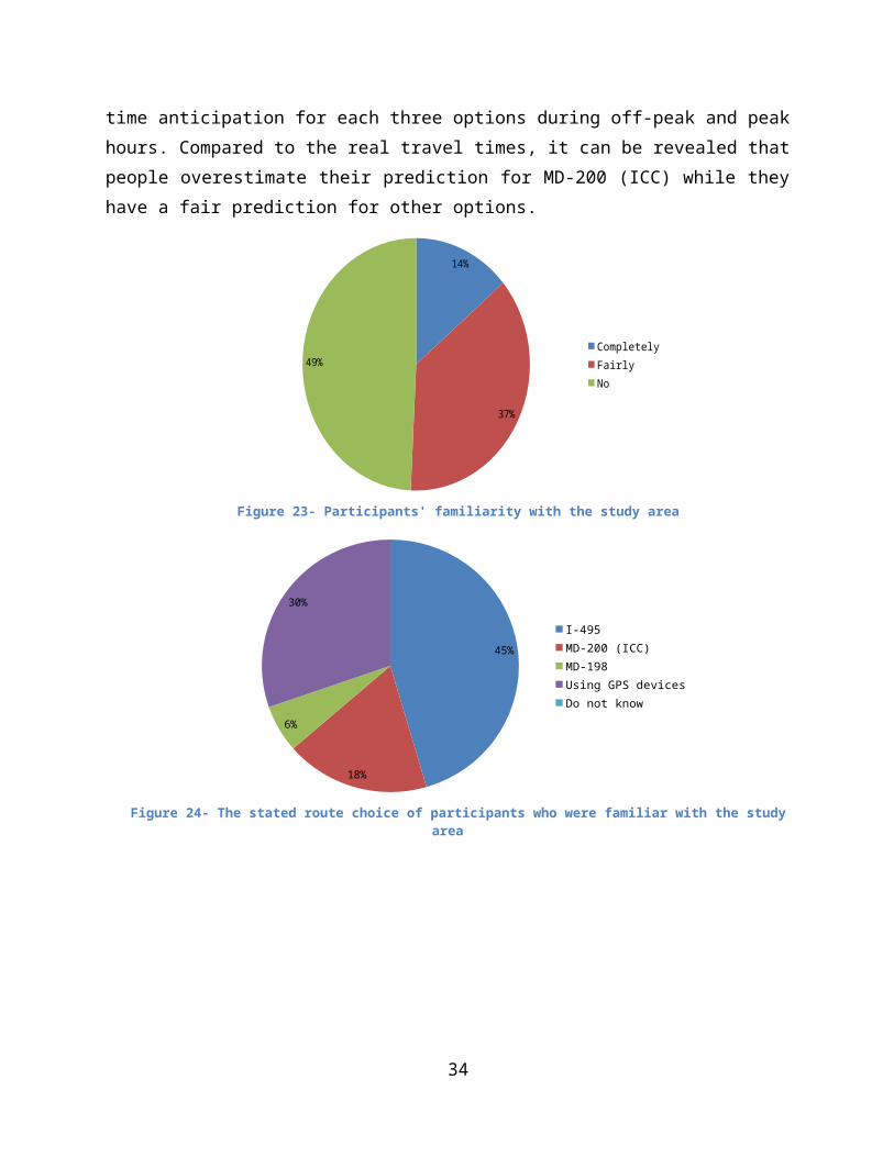
As stated in the second survey, 51 percent of the subjects were familiar with the study area completely or fairly. To take a similar journey in real world, 46 percent of them usually choose I-495 while 18 percent choose MD-200. MD-198 is the main choice for six percent of the subjects and the remaining 30 percent use their smart phones or GPS to find the best route. Figure 23 and Figure 24 show the familiarity of participants with the area and their stated route choice. Familiar participants were asked to anticipate their travel time on their stated choice during off-peak and peak hours. Figure 25 illustrates their average travel time anticipation for each three options during off-peak and peak hours. Compared to the real travel times, it can be revealed that people overestimate their prediction for MD-200 (ICC) while they have a fair prediction for other options.

14%

37%

49%CompletelyFairlyNo

Figure 23- Participants' familiarity with the study area

26

45%

18%

6%

30%

I-495MD-200 (ICC)MD-198Using GPS devicesDo not know

Figure 24- The stated route choice of participants who were familiar with the study area

MD-198 MD-200 I-4950

10

20

30

40

50

60

70

25

3339

45 45

61

off-PeakPeak

min

utes

Figure 25- The average of stated travel time anticipation for each route

Furthermore, participants were requested to state their preference about travel time provision format on a VMS message. Among all participants, 51 percent prefer an exact time to be reported while 49 percent like a range better. The distribution of participants’ preference about VMS travel time is presented in Figure 26.

27

51%49% Exact timeA range

Figure 26- Participants’ preference for travel time information provision format on VMS

Revealed Choice Analysis

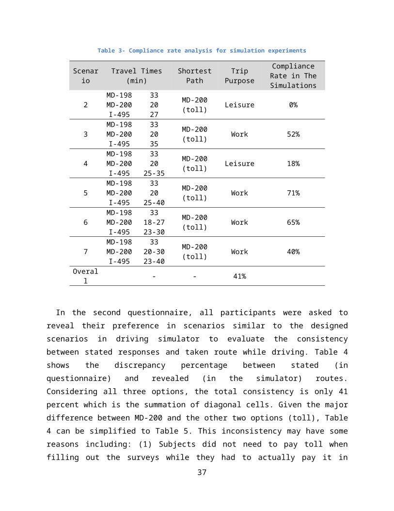
The rate of VMS compliance in each scenario is presented in Table 3. The toll road (MD-200) is the shortest path in all scenarios and the local road (MD-198)’s travel time is fixed (33 minutes) in all scenarios. Since there was no travel time information provided in scenario 1, it is excluded from this analysis. As shown, compliance rate in non-work (leisure) trips (scenario 2 and 4) was significantly lower than work trips since the participants did not have to be at the destination in a specific time and there was no penalty of late arrival to the destination.

In leisure trips, when the reliability of all routes was high and I-495 was not congested (scenario 2), nobody chose the shortest path (MD-200 toll road). Participants preferred to reach to their destination seven minutes later than pay the toll. However, when I-495 travel time increased and reliability decreased in scenario 4, more participants chose the toll road in the simulation experiment.

In work trips, when the travel time reliability of all roads were high (scenario 3) and travel difference between the shortest path and the other alternatives was high (15 and 13 minutes), 52 percent complied with the VMS in the simulator. Furthermore, when the travel time reliability of I-495 was low (scenario 5), compliance rate increased to 71 percent. This rate decreased again when the travel time reliability of shortest path decreased (scenario 6 and 7). In scenario 6, when the travel time difference between MD-200 and I-495 was 4 to 12 minutes, 65 percent of participants complied with the VMS. The compliance rate decreased to 40 percent when the reliability of MD-200 decreased to low level and there was a large overlap in MD-200 and (I-495)’s travel time ranges.

28

Table 3- Compliance rate analysis for simulation experiments

Scenario Travel Times (min) Shortest Path Trip Purpose

Compliance Rate in The Simulations

2MD-198MD-200

I-495

332027

MD-200 (toll) Leisure 0%

3MD-198MD-200

I-495

332035

MD-200 (toll) Work 52%

4MD-198MD-200

I-495

3320

25-35

MD-200 (toll) Leisure 18%

5MD-198MD-200

I-495

3320

25-40


6MD-198MD-200

I-495

3318-2723-30


7MD-198MD-200

I-495

3320-3023-40


Overall - - 41%

In the second questionnaire, all participants were asked to reveal their preference in scenarios similar to the designed scenarios in driving simulator to evaluate the consistency between stated responses and taken route while driving. Table 4 shows the discrepancy percentage between stated (in questionnaire) and revealed (in the simulator) routes. Considering all three options, the total consistency is only 41 percent which is the summation of diagonal cells. Given the major difference between MD-200 and the other two options (toll), Table 4 can be simplified to Table5. This inconsistency may have some reasons including: (1) Subjects did not need to pay toll when filling out the surveys while they had to actually pay it in driving session, similar to the real world. (2) Subjects could not see the traffic situation when reading the given travel time on surveys whereas they were able to do it while driving and it could help them sense the reported travel time reliability. First reason justifies the group that stated MD-200 as their choice but took either I-495 or MD-198 to not pay toll. Second reason explains the group that stated they would take I-495 or MD-198 to avoid the toll, even though they took MD-200 in simulation since they were afraid of possible delay due to the heavy traffic and the risk of penalty for their delay.

29

Table 4- Comparison of stated route in survey versus revealed choice in simulator

RevealedI-495 MD-200 MD-198 Total

Stat

ed

I-495 21% 16% 13% 50%

MD-200 11% 14% 6% 31%

MD-198 4% 9% 6% 19%

Total 36% 39% 25% 100%

Table 5- Comprison of stated versusrevealed choice for the ICC toll road

Revealed Not ICC ICC Total

Stat

ed

Not ICC 44% 24% 68%

ICC 18% 14% 32%

Total 62% 38% 100%

As mentioned earlier, after finishing each non-work trips in driving experiment, participants were asked of their approximate travel time. It has been shown that perceived travel time (PTT) is a reliable substitute for actual travel time (ATT) since drivers normally do not measure their actual travel time (Zhang & Levinson, 2008). The average actual travel time was 27.5 minutes and the average perceived travel time was 27.3 minutes which was close to actual travel time. Figure 27 illustrates participants’ perceived travel time in non-work trips versus the actual travel time recorded by simulator and the regression line. As shown in this plot, the bisector of the first quadrant intersects the regression line at around 26 minutes. It can be understood that drivers felt longer travel time in trips shorter than 26 minutes. On the other hand, they underestimated PTT in trips longer than 26 minutes. The small R-Squared and scattered data points indicates an uncertain travel time perception.

30

5 10 15 20 25 30 35 40 45 50 555

10

15

20

25

30

35

40

45

50

55

Regression LinePerceived Travel Time

ATT (min)

PTT

(min

)

R2 = 0.271

Figure 27- Comparison of PTT versus ATT for the simulation experiment

The average ATT and PTT for each option in each non-work scenario is shown in Figure 28. Comparing scenario 1 and scenario 2, it appears that drivers overestimated travel time under travel time information provision while they perceived a shorter TT when no information was provided in base scenario (scenario 1).

Scena

rio 1

(MD

-198

)

Scena

rio 1

(MD

-200

)

Scena

rio 1

(I-4

95)

Scena

rio 2

(MD

-198

)

Scena

rio 2

(MD

-200

)

Scena

rio 2

(I-4

95)

Scena

rio 4

(MD

-198

)

Scena

rio 4

(MD

-200

)

Scena

rio 4

(I-4

95)0.0

5.0

10.0

15.0

20.0

25.0

30.0

35.0

40.0

Actual Travel TimePerceived Travel Timem

in

Figure 28- PTT versus ATT for each option in each non-work scenario

31

PTT = ATT

In questionnaire 3, after driving experience, participants were asked about the accuracy of the travel time information provision in the simulator. The majority of participants (68 percent) believed that the reported travel time was always accurate and 29 percent stated it was correct most of the time. Only 2 percent of participants declared the provided travel time was not reliable enough. Figure 29 shows the participants’ belief toward the reliability of travel times in the simulator.

68%

29%

3%

YesMost of the timeSometimesNo

Figure 29- Participants’ belief toward travel time reliability in the driving simulator

Furthermore, since participants had experienced the network and got acquainted to the study area in the simulation experiment, they were asked to choose an option again in real trips. Figure30 presents their chosen route for this journey in real world after the driving simulation experiment. Thirty-one percent stated they will chose I-495, while 20 percent and 18 percent stated MD-200 and MD-198 will be their main option respectively. Twenty-nine percent believed that it is better to use GPS devices or smartphones to find the best route and only 2 percent had no idea about their choice. Interestingly, it appears that the probability of taking MD-200 and MD-198 after the driving simulation has increased compared to the stated route choice before the simulation experiment shown in Figure 24.

32

31%

20%18%

29%

2%

I-495MD-200 (ICC)MD-198Using GPS devicesDo not know

Figure 30- The stated route choice of participants after the driving simulation experiment

Compliance Model

A binary logit regression model was applied to the data to investigate the probability of choosing MD-200, the toll road and the fastest alternative. Some variables were defined to represent the traffic situations in the driving experiments. The travel time reliability of I-495 (Reliability_495) was considered zero in scenario 1 where no travel time information is provided, and varying from 1 to 3 in scenarios ranging from low to high reliability, respectively. A similar definition was used for the travel time reliability of MD-200 (Reliability_200). The travel time of MD-198 was a fixed value (33 minutes) in all experiments. Congestion was the other defined variable for I-495 (Congestion_495); it is a 0-1 binary variable with a value 0 if a route was not congested (e.g. having off-peak travel time), and 1 otherwise. The outcome variable in this analysis is binary and it is one if MD-200 was the participant’s choice and zero otherwise. Since no information about travel time and its reliability was provided in scenario 1, this scenario was excluded from analysis. To find the significant correlated variables, a bi-variate correlation analysis was conducted prior to the regression model and its result is shown in Table6. Socio-economic characteristics, presented in Table 2, subjects attitudes toward VMS and scenario-related variables were the initial variables. As shown, among driver-based variables, employment and annual income appeared to be highly correlated with the compliance variable. Gender, age, education level, household size, cars ownership, annual mileage, area familiarity and stated route had no association with compliance. Also information-based variables such as VMS exposure, VMS attention, opinion toward VMS and navigation devices usage were not meaningful predictors. On the other hand, trip purpose, reliability of I-495 and reliability of MD-200 found significantly correlated. Since employment and annual income were inter-correlated, employment could be excluded from the model. Table 7 presents the result of the logistic regression model using explained predictors. As presented, trip purpose was the major determiner of compliance so that drivers taking leisure trips were less likely to take MD-200 to

33

avoid the toll. In addition to trip purpose, the reliability of MD-200 itself has a positive relation with compliance: as the reliability of MD-200 decreases, the probability of taking this route decreases. On the other hand, there is a negative relation between the reliability of I-495 and compliance so that with increasing the reliability of this route, subjects were more likely to take I-495 rather than MD-200. Annual income also found to be effective to increase compliance possibility.

Table 6- Correlation of independent variables and compliance variable

Variable Significance (Two-tailed)

Decision(based on α = .05)

Gender .333 RejectAge .915 RejectEducation .384 RejectEmployment .058 *Household size .681 RejectAnnual Income .032 *Cars ownership .938 RejectAnnual mileage .549 RejectVMS exposure .474 RejectVMS attention .389 RejectVMS usefulness belief .764 RejectGPS devices usage .639 RejectArea familiarity .572 RejectStated Route .221 RejectTrip purpose .000 *Reliability of I-495 .049 *Reliability of MD-200 .016 *

Table 7- Compliance model results

Variable β Standard Error Significance Exp(β)

Trip Purpose 3.407 .758 .000 30.183Reliability_200 0.757 .445 .089 2.131Reliability_495 -.817 .363 .024 .442Annual Income .339 .136 .013 1.403

Constant -4.096 1.333 .002 .017Chi-Square = 42.611 (Significance = .000)-2 Log likelihood = 115.985Cox & Snell R Square = .307Nagelkerke R Square = .413

34

Route Choice Model

In addition to compliance model, the route choice behavior of subjects was investigated in this study using multinomial logistic regression. As mentioned earlier, subjects had three options of MD-198, MD-200 and I-495 to get the destination. I-495 was the choice of majority of subjects who were acquainted with the study area, since it is the major non-toll road. However, this route has very low travel time reliability due to recurring and non-recurring congestions. The result of applied multinomial logistic regression is presented in Table 8 with reference category of MD-200. According to this table, the probabilities of using I-495 and MD-198 are higher than that of MD-200 in leisure trips compared to work trips. Most participants prefer the major non-toll road when they do not have to be at their destination at a certain time. Travel time reliability of I-495 was found to be an important factor in this model. The probability of choosing I-495 compared to MD-200 is lower when the travel time reliability of I-495 is lower. Travel time reliability of MD-200 was not significant, and was hence omitted from the model. This could be because the reliability is high in five out of seven scenarios. Besides travel time reliability, the congestion level of I-495 affects the participants’ route choice. The probability of taking MD-200 is higher if I-495 is congested. Annual income also affects route choice behavior; subjects with lower income level (Group 1) were more likely to choose I-495 or MD-198 rather than MD-200 to avoid paying toll.

Table 8- Route choice model result

Taken Route Variable β Standard Error Significance Exp(β)I-495 Constant -3.246 .968 .001

Trip Purpose .032

Non-Work 1.713 .930 .065 5.548

Work Reference Category

Reliability of 495 .091

No information -19.161 1.361 .000 4.770E-9

Low -.036 .894 .968 .965

Medium -20.110 1.304 .000 1.847E-9

High Reference Category

Congestion of I-495 .025

Not Congested 20.993 1.457 .000 1310166238.807

Congested Reference Category

Annual Income .006

Group 1 2.673 .862 .002 14.490

Group 2 1.892 .965 .050 6.630

Group 3 2.256 .912 .013 9.547

35

Group 4 1.234 .871 .156 3.436

Group 5 1.260 .844 .136 3.525

Group 6 Reference CategoryMD-198 Constant -2.312 .948 .015

Trip Purpose .032

Non-work 2.170 .922 .019 8.760

Work Reference Category

Reliability of 495 .091

No information -19.637 1.301 .000 2.964E-9

Low -.945 .807 .242 .389

Medium -20.908 .000 . 8.314E-10

High Reference Category

Congestion of I-495 .025

Not Congested 19.158 .936 .000 209124325.724

Congested Reference Category

Annual Income .006

Group 1 2.625 .954 .006 13.804

Group 2 .648 1.191 .587 1.911

Group 3 2.944 .991 .003 18.996

Group 4 1.173 1.000 .241 3.231

Group 5 .745 .994 .454 2.106

Group 6 Reference Category

* MD-200 is reference categoryChi-Square = 92.255

-2 Log Likelihood = 116.628

Nagelkerke Pseudo R-Square = .474Cox and Snell Pseudo R-Square = .419

ConclusionThis study conducts an empirical disaggregate-level analysis of travel time reliability perception and its impact on travelers’ route choice behavior. Both SP survey and driving simulator techniques were used to evaluate the effects of driver characteristics and travel time reliability-related attributes on route choice and compliance behavior.

The advantages of utilizing a driver simulator with route choice capability include the ability to capture route choice behavior by providing full information on all possible routes, introduce different scenarios of information provision and traffic conditions, and compare participant responses under identical conditions. The study complements the driving simulator experiments with stated preference survey questionnaires.

Sixty-five participants from diverse socioeconomic backgrounds were recruited from the Baltimore metro area, and executed a total of 216 simulator runs on a 220 mi2 road network in Maryland using the driving simulator. All participants were familiar with VMS and over 42%

36

see a VMS during their daily commute. About 85% of the participants always read and some comply with the VMS message. Half of the participants were familiar with the study area. Almost half of the participants stated that they usually choose the capital beltway, I-495, to travel from the origin to the destination, 18% choose the toll road (MD-200), and only six percent choose the local road (MD-198).

Seven scenarios involving varying traffic conditions and travel time reliability levels were provided in both the SP survey and driving simulator. The results show that participants’ choices were significantly different in the simulator experiment compared to the SP survey. Very few participants take the shortest route, which is a tolled road, for leisure trips. When no information is provided, a majority of participants (57 percent) chose the capital beltway, I-495, in the driving simulator experiments. When travel time reliability of I-495 is high and it is not congested, a majority of participants (64%) chose this route. However, when the reliability of I-495 decreases and congestion increases, participants switch to other routes. For work trips, they mostly switch to the toll road (MD-200), while for leisure trips they switch mostly to the local road (MD-198).

The study developed a compliance model using binary logistic regression. The results illustrated that trip purpose, travel time reliability of the alternative routes, and household income effect VMS compliance. A route choice model was also developed using multinomial logit regression. Similar to the compliance model, trip purpose, reliability of I-495, congestion level of I-495 and household income were important explanatory factors for route choice behavior.

When no information is provided, a majority of participants chose the major non-toll route (capital beltway) in the driving simulator experiments. In the presence of information, when travel time reliability of the beltway is high and it is not congested, a majority of participants chose this route. However, when the reliability of the capital beltway decreases and congestion increases, participants switch to other routes. In work trips, they mostly switch to the toll road, which is the shortest route with high travel time reliability. However, in leisure trips they switch mostly to the local road, which has high travel time reliability but is not the shortest route. The main reason to choose the toll road for work trip was stated to get to work on time and the main reason to choose alternative routes was not to pay toll.

This study showed that travel time reliability perception significantly affects travelers’ route choice and willingness to pay. The next step of this study is to provide different scenarios of toll prices and travel time reliability to find the average willingness to pay for a reliable road. Investigating route diversion behavior could be another extension to this study.

37

Works Cited

Ardeshiri, A., Jeihani, M., & Peeta, S. (2015). Driving Simulator Based Analysis of Driver Compliance Behavior under Dynamic Message Sign Based Route Guidance. IET Intelligent Transportation Systems, 9(7), 765-772.

Bertini, R. L., & Tantiyanugulchai, S. (2003). Transit Buses as Traffic Probes: Use of Geolocation Data for Empirical Evaluation. Transportation Research Record: Journal of Transportation Research Board, 1870, 35-45.

Chen, C., Skabardonis, A., & Varaiya, P. (2003). Travel-Time Reliability as a Measure of Service. Transportation Research Record: Journal of the Transportation Research Board, 74-79.

Emam, E. B., & Al-Deek, H. (2006). Using Real-Life Dual-Loop Detector Data to Develop New Methodology for Estimating Freeway Travel Time Reliability. Transportation Research Record: Journal of the Transportation Research Board, 1959, 140-150.

FHWA. (2005). Traffic Congestion and Reliability:. US Department of Transportation, Federal HighWay Administration.

FHWA. (2006). Travel Time Reliability: Making It There On Time, All The Time. US Department of Transportation, Federal HighWay Administration.

Forum8. (n.d.). VR-Design Studio. Retrieved April 14, 2015, from http://www.forum8.com/vr_design_studio.htm

Herrera, J. C., Work, D. B., Herring, R., Ban, X., Jacobson, Q., & Bayen, A. M. (2010). Evaluation of traffic data obtained via GPS-enabled mobile phones: The Mobile Century field experiment. Transportation Research Part C, 18, 568–583.

Jeihani, M., & Ardeshiri, A. (2013). Exploring Travelers' Behavior in Response to Dynamic Message Signs (DMS) Using a Driving Simulator. Baltimore, MD: State Highway Administration.

Lin, H. E., Zito, R., & Taylor, M. A. (2005). A Review of Travel-Time Prediction in Transport and Logistics. Proceedings of the Eastern Asia Society for Transportation Studies, 5, pp. 1433-1448.

List, G. F., Williams, B., & Rouphail, N. (2014). Handbook for Communicating Travel Time Reliability Through Graphics and Tables. Institute for Transportation Research and Education North Carolina State University.

38

Liu, H. X., Recker, W., & Chen, A. (2004). Uncovering The Contribution of Travel Time Reliability to Dynamic Route Choice Using Real-time Loop Data. Transportation Research Part A, 38, 435-453.

Obuhuma, ,. J., & Moturi, C. A. (2012). Use of GPS With Road Mapping For Traffic Analysis. INTERNATIONAL JOURNAL OF SCIENTIFIC & TECHNOLOGY RESEARCH, 1(10), 120-128.

Ravi Sekhar, C., Madhu, E., Kanagadurai, B., & Gangopadhyay, S. (2013). Analysis of travel time reliability of an urban corridor using micro simulation techniques. Current Science, 105(3), 319-329.

Recker, W., Chung, Y., Park, J., Wang, L., Chen, A., Ji, Z., . . . Oh, J.-S. (2004). Considering Risk-Taking Behavior in Travel Time Reliability. California PATH: Partners for Advanced Transportation Technology.

Schwarzenegger, A., Bonner, D. E., Iwasaki, R. H., & Copp, R. (2008). State Highway Congestion Monitoring Program (HICOMP). Sacramento, Ca: Annual Data Compilation.

Sharma, S., Hsu, D.-Y., Soon, Y.-T., & Peeta, S. (2012). Development of realistic behavior models for reliable assessments of benefits from real-time traveler information provision. 13th International Conference on Travel Behaviour Research. Toronto, Canada.

Small, K. A., Noland, R., & Chu, X. (1999). Valuation of Travel Time Savings and Predictability in Congested Conditions for Highway User-Cost Estimation. National Research Counsil. Washington D.C.: Transportation Research Board.

Strategic Highway Research Program (SHRP2). (2013). Evaluating Alternative Operations Strategies to Improve Travel Time Reliability. Washington D.C.: Transportation Research Board.

van Lint, J. C., & van Zuylen, H. J. (2005). Monitoring and Predicting Freeway Travel Time Reliability Using Width and Skew of Day-to-Day Travel Time Distribution. Transportation Research Record: Journal of the Transportation Research Board, 1917, 54-62.

Zhang, L., & Levinson, D. (2008). Determinants of Route Choice and Value of Traveler. ransportation Research Record, Journal of Transportation, 81-92.

39

Appendix A: Survey Questionnaire 1

Dear Participant,

We greatly appreciate your participation in our research to evaluate the impact of route travel time reliability on driver’s route choice. Your participation is of great importance to this study. Please fill in the appropriate choice for each question.

Thank you.

1) What is your gender? * Female

Male

2) What is your age group? * 17 or below

18 to 25

26 to 35

36 to 45

46 to 55

56 to 65

More than 65

3) What is your education level? * High School

Associate degree

College

Post graduate

4) Do you work? * No

Work part time

Work full time

5) What type of driving license do you have? * Don’t have

Learner’s Permit

Permanent license for regular vehicles (class C)

Permanent license for all types of vehicles (class A)

I

6) What is your household size? * 1

2

3

4 or more

7) What is your household annual income? (Optional) Less than $20K

$20 to $30K

$30 to 50K

$50 to $75K

$75 to $100K

More than $100K

8) How many cars do your household own? * No car

1

2

3 or more

9) What is the average annual driving mileage on your own car (in miles)? * Less than 8,000

8,001 to 15,000

15,001 to 30,000

More than 30,000

10) Are you familiar with any type of Variable Message Signs (VMS), such as this image: *

Yes

No

Please read the following before answering the next set of questions if you are not familiar with VMS:

II

Variable/Dynamic Message Sign (VMS or DMS) is an electronic device providing qualitative and/or quantitative information on traffic conditions and events to travelers. Traffic congestion, accidents, work zones, alternative routes, and expected delay represent such information.

11) How often do you see a VMS on your travel? * Never

Sometimes

Everyday commute

12) To what extent do you pay attention to a VMS? * I don’t pay attention

Usually don’t get a chance to read it

Only in a few situations (such as an accident)



13) When you go to work/home, do you follow VMS messages? * Do not pay attention

Only in a few situations (such as an accident)

Read to see when I get there


Not applicable for me

14) Do you feel that VMS is a useful device for providing traffic information for travelers? *

Absolutely

Potentially

I don’t think so

15) Do you usually use GPS/smartphone for route guidance when you drive? * Never

Sometimes

Always

16) Do you usually listen to the radio traffic information when you commute? * Most of the time

Sometimes

Very few times

Never

III

Appendix B: Survey Questionnaire 2

Dear Participant,

This is the 2nd part of our survey which is more specific to the study area. Suppose you are driving on I-95 southbound (right before MD-198) and trying to reach downtown Rockville (see the figure below). Please answer the following questions.

1) Are you familiar with this origin-destination trip and its alternative routes? *

No

Somewhat

Completely familiar

As shown in the map, there are 3 major routes between the origin and the destination: I-495, MD-200, and MD-198. I-495 is a freeway but usually is congested. MD-200 is the fastest route, but it is a toll road. MD-198 is a local road with many intersections and lower speed limit.

If your answer to Question 1 is “NO”, please skip to Question 7.

2) Which route do you usually take to reach downtown Rockville form the origin point?

I-495

MD-200 (ICC)

IV

MD-198

I have no idea

I use electronic media (google, mapquest,…)

I use my GPS/smartphone

3) What is the approximate anticipated driving time from origin to destination during normal traffic? *

20 min

30 min

45 min

60 min

I have no idea

4) What is the approximate anticipated driving time from origin to destination during the peak period? *

20 min

30 min

45 min

60 min

More than 1 hour

I have no idea

5) What is your alternative route to reach downtown Rockville? *

I-495

MD-200 (ICC)

MD 198

I have no idea /Do not have any alternative route



V

6) How long does the alternative route take under normal traffic conditions (answer by comparing to the usual route)? *

Same as usual route or less

5-10 minutes

10-15 minutes

15-20 minutes

over 20 minutes

I don’t know

7) Suppose that it is the AM peak and you are going to WORK from the origin to the destination shown in the above map. Consider the following different messages being displayed on the VMS on I-95. What route will you choose under each message? Please view each message situation independently.

7-1) Rockville via MD-198, 33 minutes

MD-200, 20 minutes (toll, $4)

I-495, 27 minutes

MD-198

MD-200

I-495



I-495, 25-30 minutes

MD-198

MD-200

I-495


MD-200, 18-23 minutes (toll, $4)

VI


MD-198

MD-200

I-495




MD-198

MD-200

I-495




MD-198

MD-200

I-495




MD-198

MD-200

I-495




MD-198

VII

MD-200

I-495




MD-198

MD-200

I-495




MD-198

MD-200

I-495



I-495, 35 minutes

MD-198

MD-200

I-495



I-495, 35 minutes

MD-198

MD-200

VIII

I-495




MD-198

MD-200

I-495



I-495, 30 minutes

MD-198

MD-200

I-495

8) Suppose that it is the off peak period and you are going to do SHOPPING from the origin to the destination shown in the above map. Consider the following different messages being displayed on the VMS on I-95. What route will you choose under each message? Please view each message situation independently.



I-495, 27 minutes

MD-198

MD-200

I-495



IX


MD-198

MD-200

I-495




MD-198

MD-200

I-495




MD-198

MD-200

I-495




MD-198

MD-200

I-495

X




MD-198

MD-200

I-495




MD-198

MD-200

I-495




MD-198

MD-200

I-495




MD-198

MD-200

XI

I-495



I-495, 35 minutes

MD-198

MD-200

I-495



I-495, 35 minutes

MD-198

MD-200

I-495




MD-198

MD-200

I-495



I-495, 30 minutes

XII

MD-198

MD-200

I-495

9) Suppose that it is the AM peak and you are going to WORK from the origin to the destination shown in the above map. Assume that you were planning to take I-495 route. Consider the following different messages being displayed on the VMS on I-95. What is your willingness to change your route in the scale of 1 to 5 (1 means very low willingness and 5 means very high willingness) in each of the following messages? Please view each message situation independently.



I-495, 27 minutes

1 (very low willingness)

2

3

4

5 (very high willingness)





2

3

4


XIII





2

3

4






2

3

4






2

3

4


XIV


MD-200, 20-30 minutes (toll)



2

3

4






2

3

4



MD-200, 18-27 minutes (toll)



2

3

4

XV






2

3

4




I-495, 35 minutes


2

3

4




I-495, 35 minutes


2

3

XVI

4






2

3

4




I-495, 30 minutes


2

3

4


XVII

Appendix C: Survey Questionnaire 3

Dear Participant,

Thanks for riding our simulator! This is the last part of the survey in which we like you to share your experience with us. Please answer to the following questions.

Thanks

1) Which route will you take when you make a real trip? *

I-495

MD-200 (ICC)

MD-198

I have no idea



2) Do you think VMS information given to you in the simulator was correct? *

(VMS: Variable Message Sign)

Yes

No

Most of the time

Rarely

3) Do you prefer the VMS message to give you an exact time or a range? *

Exact time

A range

XVIII

4) Generally, will you follow VMS messages in real world in a familiar route (please check all that applies)? *

Yes, always

For work trip yes, for non-work no

It depends on the message content

It depends on many factors other than those mentioned

Never

5) Generally, will you follow VMS messages in real world in an unfamiliar route (check all applies)? *

Yes, always

For work trip yes, for non-work no

It depends on the message content

It depends on many factors other than those mentioned

Never

6) Do you think VMS is a useful device in providing traffic information for travelers? *

Yes

No

7) Do you think VMS yields correct traffic information? *

Yes

No

Most of the times

Rarely

8) What time do you usually get to work?

XIX

Example: 11:00 AM

9) How important is for you to get to work on time? *

Very Important

Not very important

Not applicable for me

XX

Appendix D: Consent Form

You are invited to participate in a study of the effect of travel time reliability on route choice decisions. We hope to learn how effective these systems are and how we can make them more effective for travelers. The study is being conducted by Dr. Mansoureh Jeihani of Morgan State University. You were selected as a possible participant in this study because you kindly responded to our invitation and accepted to participate.

If you decide to participate, we will ask you to fill out three survey questionnaire forms. You will be trained how to drive the simulator. Then you will drive the simulator several times in different traffic and driving conditions. It will take no more than 3 hours in each visit. You may participate in different days. You will be paid $12 per hour of driving the simulator. When you drive the simulator, you may feel dizzy in the first few experiments until you get used to it. There is no risk of driving the simulator, you just may feel dizzy or fatigue. You may get headache. You may find it fun to drive the simulator and have some experiences such as crashes that are dangerous in the real world.

Your decision whether or not to participate will not prejudice your future relation with the Morgan State University. If you decide to participate, you are free to discontinue participation at any time without prejudice.

Any information that is obtained in connection with this study and that can be identified with you will remain confidential and will be disclosed only with your permission.

If you have any questions, please do not hesitate to contact us. If you have any additional questions later about the study, please contact Mansoureh Jeihani at 443-885-1873 who will be happy to answer them. If you have further administrative questions, you may contact the MSU IRB Administrator, Dr. Edet Isuk, at 443-885-3447.

You will be offered a copy of this form to keep.

You are making a decision whether or not to participate. Your signature indicates that you have read the information provided above and have decided to participate. You may withdraw at any time without penalty or loss of any benefits to which you may be entitled after signing this form should you choose to discontinue participation in this study.

_________________________________________ ___________________Signature Date

_________________________________________ ___________________

Signature of Parent/Legal Guardian (If necessary) Date

_________________________________________ _____________________

Signature of Witness (If appropriate) Signature of Investigator

XXI

Executive Summary - Morgan State University · Web viewThe first questionnaire was focused on...

Documents

Transcript of Executive Summary - Morgan State University · Web viewThe first questionnaire was focused on...