Exchange Rates and Interest Parity - University of...

Exchange Rates and Interest Parity

Charles EngelUniversity of Wisconsin and NBER

DiscussionFabio Ghironi

Boston College and NBER

Handbook of International Economics Conference

National Bureau of Economic Research, September 14-15, 2012

Introduction

• This is an outstanding survey of a vast theoretical and empirical literature on the exchangerate (ER) and uncovered interest rate parity (UIP).

• With only 15 minutes, there is no short summary I could do that would do justice to thepaper, and there is no way I can discuss how Charles treats all the literature branches itreviews.

• Therefore, I will focus on the part of the literature I am most familiar with—trying tooffer suggestions on how its most significant contributions can perhaps be made moretransparent—and I will highlight a potential issue that arises when one tries to reconcile thispart of the literature with Charles’ own work with Kenneth West.

• Since I will have nothing to say about the excess return term that Charles introduces inthe UIP equation, I will eliminate that term altogether from my discussion.

– Note: This does not mean that I believe is not important.

1

New Keynesian ER Models

• The paper “identifies” the New Keynesian literature on the ER with the literature thatmodels monetary policy as endogenous interest rate setting in response to economicconditions—product price inflation in the paper’s examples—plus exogenous interest rateshocks.

• That is different from how I (and perhaps others) think of the New Keynesian literature onthe ER.

• Obstfeld and Rogoff (JPE 95—OR below) was the first New Keynesian paper on ERdynamics—the defining New Keynesian features being price setting power based onmonopolistic competition and price rigidity.

• Betts and Devereux (JIE 00—BD below) and Corsetti and Pesenti (QJE 01—CP below) areother New Keynesian papers on ER dynamics.

2

New Keynesian ER Models, Continued

• In all these papers, monetary policy is modeled as exogenous money shocks, and all thesepapers perform the classic Dornbusch (JPE 76) exercise in the context of the respectivemodels:

– Does a permanent money increase cause ER overshooting?

– Yes if the consumption elasticity of money demand is below 1 and there are deviationsfrom purchasing power parity (PPP)—non-traded goods in OR, local currency pricing(LCP) in BD.

• The key contribution of these papers to the ER literature was to provide a rigorousmicrofoundation to Dornbusch’s exercise, shedding light on the structural features of theeconomy that are important for ER overshooting when households and firms behaveoptimally.

3

New Keynesian ER Models, Continued

• In all these exercises, money demand is the centerpiece of ER determination, with the ER() determined (under assumption of separable, power utility from consumption and realmoney balances) by an equation of the form:

(1− ) = M −M∗ −1

(C − C∗ ) +

1

(+1 − ) (1)

where:

– ≡ fraction of firms that engage in LCP,

· = 0 in OR and CP (who assume full producer currency pricing—PCP) and 0 ≤ ≤ 1in BD,

– M −M∗ ≡ relative money supply,

– 1 ≡ consumption elasticity of money demand,

– C − C∗ ≡ relative consumption,

– and ≡ households’ discount rate.

• Equation (1) is combined with UIP and the other model ingredients to determine the ER inthe general equilibrium (GE) of these New Keynesian models.

4

Endogenous Interest Rate Setting

• Taylor (CR 93) changed the way we think about monetary policy by showing the abilityof a simple interest rate rule to track Federal Reserve behavior closely (under normalcircumstances).

– Woodford (Book 03) provides the most complete treatment of so-called Taylor rules inclosed economies and clarifies formally the importance of (appropriate) interest rateresponses to endogenous variables for equilibrium uniqueness, solving the indeterminacyfound by Sargent and Wallace (JPE 75) under exogenous interest rate setting.

• Over time, many in the open economy New Keynesian camp incorporated Taylor’s andWoodford’s insights in thinking about ER dynamics.

– To the best of my knowledge, Benigno and Benigno (JIMF 08—BB below) and Cavalloand Ghironi (JME 02—CG below) were the first to do it in two-country, GE models.

5

Endogenous Interest Rate Setting, Continued

• From my perspective, a first-order insight from the literature on ER dynamics withendogenous interest rate setting is that, under assumption of separability, the modelscompletely de-emphasize the role of money demand in ER determination (in fact, themodels are often “cashless”).

• It seems to me that this is an important change in how we think about ER determination thatought to be emphasized more in the paper.

6


• Consider the following simple example.

• UIP holds:

i − i∗ = +1 − where i − i∗ is the interest rate differential.

• Policy is described by:

i = + i∗ = ∗ + ∗ 0

where:

– and ∗ ≡ domestic and foreign CPI inflation rates,

– and and ∗ ≡ exogenous policy shocks (assume they follow independent (1)processes with persistence ∈ [0 1) and i.i.d., normal innovations with zero mean andequal variance).

· I assume responses to CPI inflation rather than product price inflation because itsimplifies the example (and, on positive grounds, it is quite accurate, as several centralbanks respond to CPI inflation).

• PPP holds:

− ∗ = − −1

7


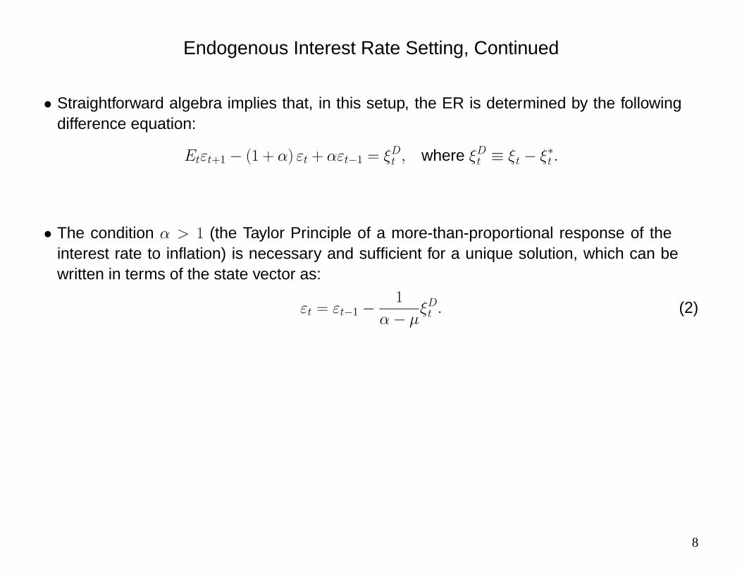
• Straightforward algebra implies that, in this setup, the ER is determined by the followingdifference equation:

+1 − (1 + ) + −1 = where ≡ − ∗

• The condition 1 (the Taylor Principle of a more-than-proportional response of theinterest rate to inflation) is necessary and sufficient for a unique solution, which can bewritten in terms of the state vector as:

= −1 −1

− (2)

8


= −1 −1

−

• Observation 1: We completely determined the ER without any reference to money demand.

• Observation 2: There is a unit root in the ER.

– This is a standard implication of interest rate setting in response to inflation rates ratherthan price levels.

– It is robust to a variety of alternative specifications (for instance, it arises also in BB,where policy responds to product price inflation, and also if policy responds to differentmeasures of output in addition to inflation).

• Observation 3: If = 0 (no persistence in exogenous interest rate shocks), the term− (− ) reduces to a normally distributed innovation with zero mean, and (2) producesrandom walk (RW) behavior for the exchange rate.

9


= −1 −1

−

• Note: A unit root in the ER and RW behavior without any assumption about any discountfactor a la Engel and West (JPE 05—EW below).

– Obviously, this does not mean that I believe this example as the theory that explainsER dynamics in reality, but it highlights certain (to me) important consequences ofendogenous interest rate setting that are not as transparent in Charles’ paper.

10


• In a more fleshed out, New Keynesian model (with PCP and Calvo JME 83 rigidity), BBconsider policy rules of the form:

i = 1y + 2

, i∗ = 1y

+ 2

∗ , 1 ≥ 0 2 ≥ 0

where y and y ≡ domestic and foreign output gaps (relative to the flexible-priceequilibrium), and the superscript denotes inflation in product prices.

• Assuming the conditions for determinacy are satisfied, there is a unique solution for the ERdescribed (under standard (1) assumptions for exogenous shocks) by:

= −1 − TOT−1 + TOT

where TOT−1 is last period’s terms of trade, TOT is the flexible-price terms of trade (a linearfunction of exogenous shocks), and is an elasticity that depends on structural parameters.

– Footnote: Given BB’s definition of the terms of trade, an increase in TOT denotes adeterioration.

• The unit root in the ER implies that the response to shocks is non-stationary as long as thepolicy rules are such that the equilibrium does not replicate the flexible-price allocation (thisrequires both 1 and 2 to be finite).

11

Endogenous Interest Rate Setting and Net Foreign Assets

• CG observed that net foreign asset dynamics where part of ER determination in the ORmodel, but they disappeared from subsequent literature that “finessed the current accountissue” (indeterminacy of the steady state and non-stationarity of net foreign assets) in theOR model by doing away with a role for the current account altogether (for instance, there isno role for the current account in BB).

– Those were the years when the consensus was that current account and net foreignasset dynamics “did not matter.”

• At the same time, we were observing the United States running current account deficits inthe 1990s and the dollar appreciating.

– In the figure, an upward movement of the exchange rate indicates appreciation.

12

1. Introduction

Obstfeld and Rogoff’s (1995) ‘‘Exchange Rate Dynamics Redux’’ was originallywritten to put forth a model of exchange rate determination with an explicit role forcurrent account imbalances. The non-stationarity of the model led most of thesubsequent literature in the so-called ‘‘new open economy macroeconomics’’ todevelop in different directions and ‘‘forget’’ the insights of the model on the dynamicrelation between the exchange rate and net foreign asset accumulation by de-emphasizing the role of the latter.1

Fig. 1 shows two well known stylized facts: the persistent and growing U.S.current account deficit over the 1990s and the likewise persistent appreciation of thedollar.2 It is a commonly held view that the advent of the ‘‘new economy’’ has beenthe most significant exogenous shock to affect the position of the U.S. economyrelative to the rest of the world in recent years. We can interpret this shock as a(persistent) favorable relative productivity shock. A story that one could tell aboutthe stylized facts in Fig. 1 is that the shock caused the U.S. to borrow from the rest ofthe world and the capital inflow generated exchange rate appreciation. This storycould be reconciled with models of exchange rate determination developed in the1970s and early 1980s. Among others, examples are Dornbusch and Fischer (1980)and Branson and Henderson (1985). If the shock is taken as permanent, the story canalso be reconciled with Obstfeld and Rogoff ’s original model. Nevertheless, the

-400

-350

-300

-250

-200

-150

-100

-50

0

50

100Q

1/1

990

Q 4

/199

0

Q 3

/199

1

Q 2

/199

2

Q 1

/199

3

Q 4

/199

3

Q 3

/199

4

Q 2

/199

5

Q 1

/199

6

Q 4

/199

6

Q 3

/199

7

Q 2

/199

8

Q 1

/199

9

Q 4

/199

9

60

70

80

90

100

110

120

130

Current account Dollar effective exchange rate

Fig. 1. The dollar and the U.S. current account.

1This is achieved either by assuming unitary intratemporal elasticity of substitution between domestic

and foreign goods in consumption as in Corsetti and Pesenti (2001) or by combining the assumptions of

complete markets and power utility. Kollmann (2001) is a recent exception to the trend, although he uses a

non-stationary model. For a survey of the literature, see Lane (2001).2Source: National Accounts and Federal Reserve, respectively. Effective dollar rate: Broad exchange

rate weighted average. Current account unit: billions of dollars.

M. Cavallo, F. Ghironi / Journal of Monetary Economics 49 (2002) 1057–10971058

Endogenous Interest Rate Setting and Net Foreign Assets, Continued

• CG brought net foreign assets back into the ER picture with a mechanism for steady-statedeterminacy and model stationarity (overlapping generations—but the same results can beobtained with other mechanisms) and endogenous interest rate setting.

• The role of net foreign assets is most easily understood under flexible prices.

13


• UIP:

i − i∗ = +1 −

• Policy rules:

i = 1y + 2 + i∗ = 1y

∗ + 2

∗ + ∗ 1 ≥ 0 2 ≥ 0

– where y and y∗ = home and foreign GDP (in units of consumption).

– Then:

i = 1y + 2

+

where the superscript denotes a cross-country differential.

• PPP:

= − −1

14


• With flexible prices, the solutions for net foreign assets and GDP can be written as:

B+1 = B + Z , (3)

y = B + Z , (4)

where B denotes net foreign assets entering period , Z is exogenous relative productivity(assumed (1)), the elasticities are functions of structural parameters, and, 0 1.

• Given the condition 2 1 for determinacy, this setup yields the following unique solution forthe ER:

= −1 + B + Z + (5)

15


= −1 + B + Z +

• Here,

≡ −12 −

• 0:

– Accumulation of net foreign assets causes home agents to supply less labor than foreign,home’s terms of trade improve, and home GDP falls relative to foreign.

• 2 − 0 because 2 1 and 0 1.

• Therefore, 0 (as long as 1 0), and a current account deficit in period − 1, resultingin B 0, appreciates the ER.

• Intuition: Accumulation of net foreign debt causes home GDP to rise relative to foreign;home policy responds by increasing the interest rate (as long as 1 0), and the currencyappreciates.

16


• Under sticky prices:

= −1 + B + y−1 + Z +

(6)

– This can be rewritten replacing y−1 with the past terms of trade to yield an ER solutionsimilar to that in BB, with net foreign assets as the additional endogenous state.

• CG show that, in this case, a permanent relative productivity shock will cause externalborrowing (because sticky prices cause relative GDP to rise gradually to its new long-runlevel) and ER appreciation.

• Obviously, not a quantitative theory of what happened to the U.S. current account and ER inthe 1990s (no capital, thus borrowing only if productivity shock is permanent under stickyprices), but we viewed this as a starting point to go back to having net foreign assets in theER picture along with endogenous monetary policy.

17


• CG also show how (5) or (6) can result in hump-shaped responses of the ER to shocks (orresponses that are very similar to a RW, depending on scenarios).

– Endogenous interest rate setting has implications for Eichenbaum and Evans (QJE 95)and the literature that followed—as noted first by McCallum (JME 94).

• The fact that endogenous interest rate setting introduces a unit root in the exchange rateand can produce simulated ER paths that display RW behavior or humps (dependingon assumptions on shocks, policy, and parameter values) is, to me, another importantcontribution of this literature that perhaps deserves more explicit emphasis in the paper.

– I view the insights from this theoretical literature (BB, CG, and others) as the startingpoint for understanding the empirical results in Molodtsova, Nikolsko-Rzhevskyy, andPapell (JME 08, JMCB 11) and Molodtsova and Papell (JIE 09).

18

The Engel-West Theorem with Endogenous Interest Rate Setting

• Return to the ER equation from the OR-CP-BD framework:

(1− ) = M −M∗ −1

(C − C∗ ) +

1

(+1 − )

• Define:

f ≡ M −M∗ −1

(C − C∗ ) ≡ 1

1 + (1− ) and f ≡

f1−

• Then:

= +1 + (1− ) f (7)

• This is the ER equation at the center of EW.

19

The Engel-West Theorem with Endogenous Interest Rate Setting, Continued

• When = 1 (log utility from money) and = 0 (no LCP firms, PPP holds), equation (7)reduces to

= +1 + (1− ) f

where is the household’s discount factor:

≡ 1

1 +

• This is the OR case.

• In this case, the discount factor that approaches 1 in the EW theorem () has the “natural”interpretation of household discount factor.

– → 1 poses its own problems for the solution of intertemporal utility maximization, but itis reasonable to think that is very close to 1.

• Charles argues that equation (7) can be obtained also when we consider monetary policythrough interest rate setting.

• But there is a subtle issue that perhaps deserves some attention in that case.

20


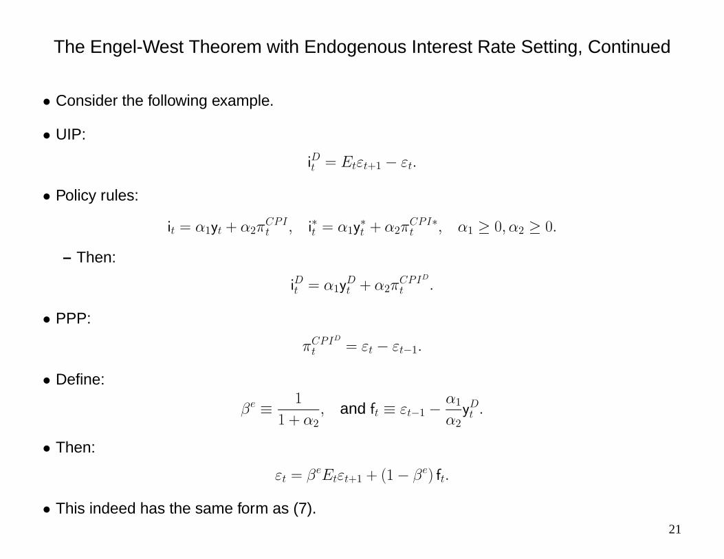
• Consider the following example.

• UIP:

i = +1 −

• Policy rules:

i = 1y + 2 i∗ = 1y

∗ + 2

∗ 1 ≥ 0 2 ≥ 0

– Then:

i = 1y + 2

• PPP:

= − −1

• Define:

≡ 1

1 + 2 and f ≡ −1 −

12y

• Then:

= +1 + (1− ) f

• This indeed has the same form as (7).21


= +1 + (1− ) f

• Should the fact that f includes the past ER be a concern when I think in terms of the EWapproach and theorem?

• More importantly, consider what it means for → 1:

• ≡ 1(1 + 2)→ 1 if and only if 2 → 0.

• But 2 is the response coefficient to inflation in the policy rules, and the Taylor Principlerequires 2 1.

– If prices are sticky, 2 1 is necessary and sufficient for determinacy in this setup when1 = 0.

– Conditions for determinacy are marginally more complicated when 1 0, but 2 1

has become a “consensus” ingredient of monetary policy.

22


• Moreover, we saw before that we do not need → 1 for the ER to feature a unit root (andbehavior potentially very close to a RW) with endogenous interest rate setting.

– In fact, in the simplest example above, we needed 2 1 to ensure that (2) was theunique solution for the ER.

23


• Where does this leave us when considering the EW theorem in relation to ER determinationunder endogenous interest rate setting?

• Can the EW theorem really be reconciled with endogenous interest rate setting?

• Footnote: I could make the same argument above in an example without PPP.

24

Conclusion

• Outstanding survey, and I learned much from reading it.

• I hope these comments will be useful to accomplish a perhaps more effective treatment ofthe New Keynesian literature (without and with endogenous interest rate setting).

25

Exchange Rates and Interest Parity - University of...

Documents

Transcript of Exchange Rates and Interest Parity - University of...