Excess Water Production Diagnosis in Oil Fields Using ...
121
Faculty of Science and Engineering Department of Mathematics and Statistics Excess Water Production Diagnosis in Oil Fields Using Ensemble Classifiers Minou Rabiei This thesis is presented for the Degree of Doctor of Philosophy of Curtin University October 2011
Transcript of Excess Water Production Diagnosis in Oil Fields Using ...

Faculty of Science and Engineering Department of Mathematics and Statistics
Excess Water Production Diagnosis in Oil Fields Using Ensemble Classifiers
Minou Rabiei
This thesis is presented for the Degree of Doctor of Philosophy
of Curtin University
October 2011

1
Declaration
To the best of my knowledge and belief this thesis contains no material previously
published by any other person except where due acknowledgment has been made. This
thesis contains no material which has been accepted for the award of any other degree or
diploma in any university.
Name: Minou Rabiei
Signature: Date: 26/10/2011

2
Abstract
In hydrocarbon production, more often than not, oil is produced commingled with
water. As long as the water production rate is below the economic level of water/oil ratio
(WOR), no water shutoff treatment is needed. Problems arise when water production rate
exceeds the WOR economic level, producing no or little oil with it. Oil and gas companies
set aside a lot of resources for implementing strategies to effectively manage the production
of the excessive water to minimize the environmental and economic impact of the produced
water.
However, due to lack of proper diagnostic techniques, the water shutoff technologies
are not always proficiently applied. Most of the conventional techniques used for water
diagnosis are only capable of identifying the existence of excess water and cannot pinpoint
the exact type and cause of the water production. A common industrial practice is to
monitor the trend of changes in WOR against time to identify two types of WPMs, namely
coning and channelling. Although, in specific scenarios this approach may give reasonable
results, it has been demonstrated that the WOR plots are not general and there are
deficiencies in the current usage of these plots.
Stepping away from traditional approach, we extracted predictive data points from
plots of WOR against the oil recovery factor. We considered three different scenarios of
pre-water production, post-water production with static reservoir characteristics and post-
water without static reservoir characteristics for investigation. Next, we used tree-based
ensemble classifiers to integrate the extracted data points with a range of basic reservoir
characteristics and to unleash the predictive information hidden in the integrated data.
Interpretability of the generated ensemble classifiers were improved by constructing a new
dataset smeared from the original dataset, and generating a depictive tree for each ensemble
using a combination of the new and original datasets. To generate the depictive tree we
used a new class of tree classifiers called logistic model tree (LMT). LMT combines the
linear logistic regression with the classification algorithm to overcome the disadvantages
associated with either method.
Our results show high prediction accuracy rates of at least 90%, 93% and 82% for the
three considered scenarios and easy to implement workflow. Adoption of this methodology
would lead to accurate and timely management of water production saving oil and gas
companies considerable time and money.

3
Acknowledgements
First and foremost, I would like to thank my supervisor, Dr Ritu Gupta, for her
continuous support and encouragement throughout my PhD. I am forever thankful to
her for introducing me to the wonderful world of statistics. Her knowledge and
valuable inputs enabled me to complete this work.
I am greatly indebted to the CSIRO, especially Dr Edson Nakagava and Dr
Gerardo Sanchez Soto for recognizing my potential, granting me a scholarship for
my research and providing technical support whenever I needed.
Special thanks to Dr Yaw Peng Cheong for his hard work towards the
simulations carried out in this work. I greatly appreciate his help and support
throughout this research.
I am grateful for the never ending love and encouragement from my parents, my
brother and my sister.
And finally, the most important thanks go to my husband, Vamegh, for his
endless help, support and encouragement and my two lovely sons, Shayan and
Novian. Thank you for your love, your patience and your understanding. Without
you beside me, I wouldn’t have been able to finish this work.

4
To Vamegh, who has always been a great inspiration to me,
To Shayan, who has been eagerly looking forward to see mum without her laptop,
and
To Novian, who has been with me in every step of writing this thesis!

5
Contents
Page
Abstract ............................................................................................................................ 2
Acknowledgements .......................................................................................................... 3
List of Figures .................................................................................................................. 8
List of Tables ................................................................................................................. 11
Nomenclature ................................................................................................................. 12
Chapter 1 Introduction
1.1 Excess water production in oil wells ................................................................ 13
1.2 Research objectives ........................................................................................... 15
1.3 Significance of the research .............................................................................. 15
1.4 Research structure ............................................................................................ 16
Chapter 2 Excess Water Production: Mechanisms and Diagnosis
2.1 Problematic water and different types of water production mechanisms ... 18
2.2 Conventional tools and techniques for WPM diagnosis ................................ 23
2.2.1 Well testing and logging techniques for diagnosing WPMs ................... 27
2.2.2 Analytical and empirical techniques for diagnosing WPMs ................... 28
2.2.3 Limitations of conventional WPMs diagnostic techniques ..................... 36
2.3 Application of data mining techniques and expert systems in water production
management ....................................................................................................... 39
2.3.1 Application of classification trees in water production management ..... 44
2.4 Summary ............................................................................................................ 45
Chapter 3 Simulation of Water Production Mechanisms
3.1 Base case simulation models for water coning ................................................ 47

6
3.1.1 Bottom water drive .................................................................................. 47
3.1.2 Edge water drive ...................................................................................... 48
3.2 Base case simulation models for water channelling ....................................... 49
3.2.1 Water injection ........................................................................................ 49
3.2.2 Edge water drive ...................................................................................... 51
3.2.3 Bottom water drive with baffles in vertical direction .............................. 52
3.3 Input parameters for simulation runs ............................................................. 52
3.4 WOR diagnostic plots ....................................................................................... 55
3.4.1 Plots of WOR against the oil recovery factor .......................................... 57
3.5 Summary ............................................................................................................ 59
Chapter 4 Classification Models: Algorithms and Evaluations
4.1 Learning and validation datasets for classification models ........................... 60
4.2 Defining the WPMs classification problem ..................................................... 64
4.3 Learning algorithms for classification models ................................................ 66
4.3.1 Classification trees ................................................................................... 66
4.3.2 Logistic model trees ................................................................................ 68
4.3.3 Ensemble classifiers ................................................................................ 69
4.3.4 Unifying ensemble classification models using a depictive tree ............. 72
4.4 Classification models performance measures ................................................. 74
4.4.1 Margin of predictions .............................................................................. 76
4.4.2 Proximity measure ................................................................................... 76
4.4.3 Outliers .................................................................................................... 76
4.4.4 Parameter importance .............................................................................. 77
4.4.5 Classification accuracy ............................................................................ 77
4.4.6 Sensitivity ................................................................................................ 78
4.4.7 Kappa coefficient ..................................................................................... 78
4.4.8 Area under ROC curves (AUC) .............................................................. 79
4.5 Summary ............................................................................................................ 79

7
Chapter 5 Results and Discussion
5.1 Evaluation of the random forest models ......................................................... 81
5.1.1 Model appraisal ....................................................................................... 81
5.1.2 Performance accuracy ............................................................................ 91
5.1.3 Consistent classification .......................................................................... 93
5.2 Comparison of random forest algorithm to other ensemble classification
techniques ........................................................................................................... 95
5.3 Evaluation of the depictive trees ...................................................................... 96
5.3.1 Evaluation and comparison of the depictive trees using new and combined
datasets .................................................................................................... 97
5.3.2 Evaluation of the depictive trees compared to RanFo models .............. 101
5.4 Discussions ....................................................................................................... 103
5.5 Summary .......................................................................................................... 105
Chapter 6 Conclusions, Contributions and Future Works
6.1 Summary of the work ..................................................................................... 107
6.2 Contributions ................................................................................................... 109
6.3 Future work ..................................................................................................... 110
References ................................................................................................ 112
Appendix A Sample R codes .................................................................................... 118

8
List of figures Page
Figure 2.1 Water management system in oil and gas fields ................................................ 20
Figure 2.2 An example of a mechanical related problem ................................................... 21
Figure 2.3 Examples of completion related problems ......................................................... 22
Figure 2.4 Examples of reservoir related problems ............................................................. 23
Figure 2.5 An example of a recovery plot used for estimating the ultimate production without
water control treatments ..................................................................................... 29
Figure 2.6 An example production history plot ................................................................... 29
Figure 2.7 An example production decline curve ................................................................ 30
Figure 2.8 Inflow and outflow performance curves for nodal system analysis ................... 31
Figure 2.9 Multi-layer channelling WOR and WOR derivatives ........................................ 33
Figure 2.10 Bottom-water coning WOR and WOR derivatives ............................................ 34
Figure 2.11 Example type curves for different values of viscosity ratio (M) ........................ 34
Figure 2.12 Example WOR plots showing the effect of a thief zone on the predicted recovery
before water breakthrough with different heterogeneity index (KHR) .............. 35
Figure 3.1 Base case simulation model for water coning from bottom water drive; (a) the
aquifer is represented by the red grid blocks with high porosity value of 2000, (b)
shows the water cone moving towards the well ................................................. 48
Figure 3.2 Base case simulation model for water coning from edge water drive; (a) the aquifer
is represented by the red grid blocks, (b) shows the water cone moving towards the
well ..................................................................................................................... 48
Figure 3.3 Base case simulation model for water channelling from water injection; (a) the
permeability model for scenario Ch-I-1 shows three flow units separated by two
low permeability layers, (b) shows the injected water gradually advancing towards
the producer, (c) gravity dominated flow between injector and producer where the
low permeability layers are removed, (d) the permeability model for scenario Ch-I-
2 with large drainage area, (e) the permeability model for scenario Ch-I-3 with large
drainage area and four flow units ....................................................................... 50
Figure 3.4 Base case simulation model for water channelling from edge water drive; (a) the
permeability model for scenario Ch-E-1 shows three flow units separated by two
low permeability layers, (b) shows the edge water gradually advancing towards the
producer, (c) the permeability model for scenario Ch-E-2 with four flow units...51
9
Figure 3.5 Base case simulation model for bottom water drive with baffles in vertical
direction; (a) the impermeable spheres modelled as zero transmissibility and
randomly distributed, (b) the bottom water flowing upward around the impermeable
spheres and gradually sweeping the oil towards the producer ........................... 52
Figure 3.6 Relative permeability curves used for different wettability scenarios ............... 54
Figure 3.7 Samples plots of the WOR and WOR derivative against time for each simulated
water production mechanism type; (a) bottom water drive coning, (b) edge water
drive coning, (c) water channelling due to injection, (d) edge water drive
channelling, (e) bottom water drive with baffles ................................................ 57
Figure 3.8 Samples plots of the WOR and WOR derivative against oil recovery factor for each
simulated water production mechanism type; (a) bottom water drive coning, (b)
edge water drive coning, (c) water channelling due to injection, (d) edge water drive
channelling, (e) bottom water drive with baffles ................................................ 58
Figure 4.1 Split points on a WOR plot ................................................................................ 62
Figure 4.2 Sample structure of a classification tree with five classes of A, B, C, D and E and
two predictor parameters of x and y ................................................................... 67
Figure 4.3 Sample structure of a LMT tree with two classes of C1, C2 and two predictor
parameters of x1 and x2 ..................................................................................... 68
Figure 4.4 Sample structure of an ensemble classification algorithm ................................. 69
Figure 4.5 The flowchart of the procedure used for developing WPMs classification models
............................................................................................................................ 75
Figure 5.1 Section of a tree from the RanFo ensemble models; at each node the cases with split
parameter values less than the splitting point go to the left daughter node and the
rest go to the right daughter node ....................................................................... 82
Figure 5.2 Margins of predictions for cases by example RanFo models from pre and
post-water-production ......................................................................................... 83
Figure 5.3 Multi-dimensional scaling plot of proximity measure from (a) Mode#0, (b)
Model#1 and (c) Model#1* ................................................................................ 85
Figure 5.4 Outlier cases identified by example RanFo models in pre and post-water-production
scenarios ............................................................................................................. 86
Figure 5.5 Variable importance plots based on Model#0; plots (a–d) show the importance of
the parameters with respect to each WPM and plot (e) shows the importance of the
parameters in overall classification .................................................................... 87

10
Figure 5.6 Variable importance plots based on Model#1, plots (a–d) show the importance of
the parameters with respect to each WPM and plot (e) shows the importance of the
parameters in overall classification .................................................................... 88
Figure 5.7 Partial dependence plots of the predictor parameters on Channelling problem based
on Model#1 ......................................................................................................... 89
Figure 5.8 Partial dependence plots of the predictor parameters on Coning problem based on
Model#1 .............................................................................................................. 90
Figure 5.9 Total classification accuracy results of the RanFo models ................................ 92
Figure 5.10 Kappa coefficient values of the RanFo models .................................................. 92
Figure 5.11 Sensitivity results of the RanFo models with respect to water production
mechanisms ........................................................................................................ 93
Figure 5.12 The sequential classification votes allocated to each case using RanFo models in pre
and post-water-production scenarios .................................................................. 94
Figure 5.13 The structure of a developed depictive tree model ............................................. 97
Figure 5.14 AUC values corresponding to depictive-new models ...................................... 100
Figure 5.15 AUC values corresponding to depictive-combined models ............................. 101
Figure 5.16 Sensitivity rates results of the depictive trees trained on the combined data ... 102

11
List of Tables Page
Table 2.1 Produced water management costs (After Jackson and Myer 2003) ................. 19
Table 2.2 Excess water production problems categorized based on their treatment difficulty
(After Seright et al. 2003) ................................................................................... 20
Table 2.3 Water production mechanisms, diagnosis and solutions .................................... 25
Table 2.4 Typical characteristic behaviour of each mechanism of water invasion ............ 38
Table 2.5 Failure mode and effect analysis for water production problems ...................... 41
Table 3.1 The Corey exponents and endpoints used for generating relative permeability
curves for different wettability scenarios ........................................................... 53
Table 3.2 Oil, water and gas PVT properties for different API values ............................. 54
Table 3.3 Mobility ratios calculated from relative permeability and viscosity .................. 55
Table 4.1 Reservoir characteristics selected as input into the classification models ......... 61
Table 4.2 Response and predictor parameters forming each case of WPMs ..................... 64
Table 4.3 The confusion matrix corresponding to classification of WPMs ....................... 77
Table 5.1 Performance comparison between random forest, bagging and AdaBoost
classification algorithms based on total accuracy and Kappa. The last column
presents the P-value for comparing the accuracy across RanFo, bagging and
AdaBoost methods using a chi-square test. ........................................................ 96
Table 5.2 The logistic regression equations for each terminal node in the developed depictive
tree shown in Figure 5.13 ................................................................................... 98
Table 5.3 A comparison of performance between depictive-new and depictive-combined
models in terms of accuracy and Kappa values. The last column presents the
P-value for comparing accuracy across RanFo, bagging and AdaBoost methods
using a chi-square test ........................................................................................ 99
Table 5.4 The sensitivity values of the depictive trees trained on new and combined data with
respect to the WPM type .................................................................................. 100
Table 5.5 A comparison of performance between random forest algorithm and
depictive-combined models in terms of accuracy and Kappa values ............... 102

12
Nomenclature
jC Code for the corresponding WPM
oC Oil exponent
wC Water exponent
mD Dynamic predictor parameter
i Index of predictor parameters
)(yI jr Indicator parameter corresponding to the labels for each WPM
J Index of cases
K Number of cases in the dataset
eoK Effective permeability to oil
ewK Effective permeability to water
hK Horizontal permeability
vK Vertical permeability
roK Oil relative permeability
rwK Water relative permeability
L Dataset
L’ New dataset generated for the depictive tree
ijL Learning dataset
m Number of dynamic predictor parameters
M Mobility ratio
oµ Oil viscosity
wµ Water viscosity
n Number of static predictor parameters
N Number of cases
€
NP Produced oil
iP Proportion of cases in each class
nS Static predictor parameter
orwS
Residual oil saturation
wcS Connate water saturation
φV Pore volume

Chapter 1 Introduction
13
Introduction
1.1 Excess water production in oil wells
Excessive water production is one of the common and challenging problems
associated with hydrocarbon production. Reservoir rocks normally contain both
petroleum hydrocarbons and connate water. Once the production starts, this water called
connate water is also produced into the wellbore comingled with oil. In addition to the
connate water contained in reservoir rocks, many petroleum reservoirs are bounded by
or are adjacent to large aquifers. These aquifers can provide the natural drive for
petroleum production. Once the aquifer pressure is depleted, additional water is also
injected into the reservoir to provide further pressure to the hydrocarbon reserves to
move towards the production wells. Water from these various sources can flow into the
wellbore and co-produced with the hydrocarbon stream. Such water is referred to as
produced water. The ratio of produced water to the produced oil is denoted as WOR
(water/oil ratio). The WOR economic limit is where the cost of handling and disposal of
the produced water approaches the value of the produced oil.
The water produced in to the well bore comingled with oil at an economic water/oil
(WOR) ratio is an accepted fact in the oil industry as it cannot be reduced or shut off
without affecting the oil production. Problems arise when water flows in to the oil well
at a rate exceeding the economic WOR limit, producing little or no oil. The cost of
handling and disposing this unwanted water could have a negative impact on the
economic life of the oil well. It is estimated that on average oil companies produce three
barrels of water for each barrel of oil, which entails a staggering cost of US$ 30-40
billion worldwide (Du et al. 2005).
In addition to the direct cost of handling the produced water, it also has negative
impacts on the overall productivity rates. Excessive water production reduces the net oil
production rate, increases corrosion rates in the production system and may eventually
lead to early abandonment of the affected wells. The environmental issues in connection
with water production are another concern for oil companies. They have to comply with
strict environmental regulations regarding water treatment and disposal facilities, which
1

Chapter 1 Introduction
14
consequently increases production costs.
Water is produced in to the well due to many different causes. Water production can
be related to mechanical problems, poor completion procedures or reservoir conditions.
The main obstacle in the management of water production studies is the correct
diagnosis of the nature and the origin of the problems. Each problem type requires a
different approach to control and treat the problem effectively. In reality, an oil well can
experience a combination of different problem types. However, reservoir related
problems of coning and channelling through high permeability layers are more
challenging to diagnose and treat (Seright et al. 2003).
The mechanism and the volume of the water produced into a wellbore mainly
depends on petrophysical properties, pressure and temperature conditions of the
reservoir, geometry and conditions of the aquifers, trajectory and location of the drilled
wells within reservoir structure, type of completion and stimulation methods.
Depending on the characteristics of the reservoir, type of the diagnosed problem and
objectives of the water production treatment, a variety of mechanical, chemical and well
construction techniques can be applied to stop or reduce the flow of water into the
wellbore. However, the water production mechanism (WPM) must be properly
investigated and accurately diagnosed in order to design an appropriate and effective
treatment method. Incorrect, inadequate, or lack of proper diagnosis usually leads to
ineffective water control treatments.
Several analytical and empirical techniques using information such as production
data, water/oil ratio and logging measurements have been developed to determine the
type of water production problem, locating the water entry point in the well and
choosing the candidate wells to perform treatment methods. Water/oil ratio diagnostic
plots are probably the most widely used technique in reservoir performance studies.
Many oil companies to date rely on log/log plots of WOR and its derivative against time
to identify WPMs caused by water coning or channelling (Al Hasani et al. 2008;
Sanchez et al. 2007). WOR diagnostic plots are easy to use and explicable for non-
experts. The production data required for these plots are routinely collected and
accuracy of these data is usually reliable. Nevertheless, without taking other important
reservoir parameters in to account, the WOR diagnostic plots could easily be
misinterpreted and it has been demonstrated that applying these plots on their own could
be misleading (Seright 1998, Rabiei et al. 2009, 2010a, 2010b).
In view of the fact that proper diagnosis of WPMs is a vital step in reservoir

Chapter 1 Introduction
15
performance studies and considering that water/oil production data are the most
commonly available data, we develop a novel approach in applying WOR data for
discriminating WPMs in oil wells. Instead of plotting the WOR against time, we explore
plots of WOR against the oil recovery factor and extract predictive data points from
these plots. Modern statistical classification techniques are then applied to integrate the
extracted WOR points with reservoir parameters to build classification models. These
classification models are used for identifying WPMs due to coning, channelling or
water segregation problems in oil wells.
1.2 Research objectives
The main objectives of this research can be summarized as follows:
• To explore and extract useful information for classification purpose from plots of
WOR versus the oil recovery factor for different WPMs. For this purpose, synthetic
reservoir models are built to simulate excess water production due to coning,
channeling and gravity segregated flows.
• To investigate various classification techniques for generating sophisticated WPM
classification models.
• To develop rigorous classification models, which integrate the extracted WOR
values with selected reservoir characteristics, for identifying WPMs. Modern
ensemble and non-ensemble tree-based classification techniques are employed and
the results are compared in different scenarios of pre-water production, post-water
production with static reservoir parameters and post-water production without
static reservoir parameters.
1.3 Significance of the research
• This research addresses the need for a proper technique for diagnosing excess
water production in oil wells. Research shows that despite the general agreement
on such requirement in the petroleum industry, only limited efforts on developing
specific diagnostic techniques for identifying WPMs are available.
• As oil fields mature, the problems encountered in the hydrocarbon production
become increasingly complex and require more sophisticated approaches to solve.
In addition to this, a hydrocarbon reservoir usually experiences a number of
problems simultaneously, which adds to the difficulty of identifying the causes of

Chapter 1 Introduction
16
the problems. This research provides a multidisciplinary approach in diagnosing
excess water production in oil wells integrating information from reservoir
characterization studies with the knowledge gained from dynamic production
data.
• WOR diagnostic plots have been commonly used for excess water diagnosis, in
spite of the fact that these plots are not general and not applicable in all conditions
to identify the WPMs. In this work, we presents an advancement of WOR
diagnostic plots in which we use the oil recovery factor instead of time and extract
predictive data points from the plots. This approach provides adequate
information required for studying different WPMs and eliminates the need for
handling large amounts of irrelevant data. Consequently, it can be used as a cost
effective tool for WPM diagnosis.
• Using sophisticated mathematical and data mining techniques, our approach offers
great benefits to the oil industry by extracting implicit, previously unknown and
potentially useful information from the huge amounts of raw data. The applied
techniques help in reducing the uncertainties associated with data analysis and
interpretations, and hence lowering the risk of misdiagnosis of a problem.
• The results obtained from our study confirm that our approach can successfully
identify different types of WPMs. This effectual WPM diagnostic tool, can
promote the economic life of a producing well by correctly identifying the source
of the water production problem. Furthermore, by predicting the possibility of
encountering specific water production problems in the future, it can facilitate the
planning of a proactive solution to the likely problems.
1.4 Research structure
This study is divided in to six chapters: chapter one briefly explains the process of
excess water production in oil wells and problems associated with it. It states the
research objectives and significance of this work. In chapter two, we provide a review
of the available literature on WPMs and introduce different types of WPMs. Chapter
two also describes the current diagnostic techniques practiced in the industry for excess
water production identification and states the shortcomings of these techniques. It also
presents a concise review of the data mining techniques used in the water management
studies. Chapter three provides a detailed description of reservoir simulation models

Chapter 1 Introduction
17
developed for this study. The main emphasis of this chapter is on examining the WOR
plots associated with each problem type and to highlight the limitations of such plots in
problem recognition. This chapter provided the information for developing database for
developing classification model. In chapter four, we explain our proposed methodology
in utilizing WOR diagnostic plots and describe the anticipated framework for
developing statistical models. Chapter five presents the results obtained from the
generated classification models and gives a comparative examination of each statistical
technique. Chapter 6 provides the conclusions from this study and recommendations for
future works.

Chapter 2 Excess Water Production: Mechanisms and Diagnosis
18
Excess Water Production: Mechanisms and Diagnosis
This chapter presents the water production problems commonly encountered in
petroleum production. Here in, we also present the key challenges in detecting and
managing the water production mechanisms (WPM). In section 2, we first explain what
is regarded as excess water production and provide a brief review on different types of
water production mechanisms (WPM) encountered in oil fields. Conventional
diagnostic tools and techniques including analytical and empirical methods for detecting
and management of WPMs are presented in section 2.2. Section 2.3 discusses modern
data mining techniques with a focus on classification trees and presents examples of
their successful application in water production management and related issues. In
section 2.4, a summary review of the literature and our intended approach in WPMs
diagnosis is presented.
2.1 Problematic water and different types of water production mechanisms
Water is an inevitable by-product of oil production. It is one of the natural sources
of reservoir energy causing the hydrocarbon flow into the wellbore. In a water drive
reservoir, the water in an adjacent aquifer moves into the reservoir, and sweeps the oil
towards the wellbore. When the water drive is not strong, additional water is injected
into the reservoir to maintain reservoir pressure and aid the movement of oil. As the
oilfield matures, this sweep water is produced into the wellbore comingled with oil.
Production of this water cannot be stopped without affecting the oil rate. Providing that
the water production rate is below the WOR economic level, no water shutoff treatment
is needed. Problems arise when water breaks into the wellbore prematurely or when
water production rate exceeds the WOR economic level, producing no or little oil with
it. This type of water is usually referred to as “bad water” or “produced water” (Bailey
et al. 2000; Reynolds 2003; Veil et al. 2004).
2

Chapter 2 Excess Water Production: Mechanisms and Diagnosis
19
In a study by Khatib and Verbeek (2003), it was estimated that oil companies
produce a global average of 210 million bbl of water each day. The total volume of
produced water in the United States estimated for 2007 was about 21 billion bbl, equal
to an average of 57.4 million bbl/day (Clark and Veil 2009). The cost of managing the
produced water is an important component of the overall cost of producing oil. Arentz
(2008) considered a conservative estimate of approximately 1 US$/m3 for handling
produced water including the lift, treatment and discharge. Since the produced water
contains undesirable components that are environmentally unfriendly, it requires
treatment before disposal. Water can also cause corrosion and scale deposition in the
equipment, which as a result require more maintenance or even replacement. The water
control treatments including mechanical or chemical techniques are also a big
expenditure in fields with excess water production problems. Jackson and Myers (2003)
estimated the average cost of disposal methods for the produced water as presented in
Table 2.1.
Table 2.1 Produced water management costs (After Jackson and Myers 2003)
Management Option Estimated Cost ($/bbl)
Surface discharge 0.01–0.8 Secondary recovery 0.05–1.25 Shallow reinjection 0.1–1.33 Evaporation pits 0.01–0.8 Commercial water hauling 1–5.5 Disposal wells 0.05–2.65 Freeze-thaw evaporation 2.65–5 Evaporation pits and flow lines 1–1.75 Constructed wetlands 0.001–2 Electrodialysis 0.02–0.64 Induced air flotation for de-oiling 0.05 Anoxic/aerobic granular activated carbon 0.083
Excessive water production affects the economic viability of many oilfields
worldwide. The negative impacts of excess water production include loss of revenue
because of decreased oil production, unnecessary expense of lifting water from wellbore
to the surface and cost of water treatment facilities and water disposal systems. A total
water management system can be pictured as shown in Figure 2.1 (Arnold et al. 2004).
WPMs have been classified in the literature using different criteria depending on
the author’s interests and purpose of the work. The classification based on the degree of
the treatment difficulty is more applicable in studies related to the design and
application of the water control strategy (Bailey et al. 2000; Seright et al.2003). For

Chapter 2 Excess Water Production: Mechanisms and Diagnosis
20
example, Seright et al. (2003) categorized the water production problems based on the
difficulty of treatment (Table 2.2).
Figure 2.1 Water management system in oil and gas fields (After Arnold et al. 2004) Table 2.2 Excess water production problems categorized based on their treatment difficulty (After Seright et al. 2003)
Category A: “Conventional” treatments
• Casing leaks without flow restrictions • Flow behind pipe without flow restrictions • Non fractured wells (injector or producers) with effective barriers to
crossflow
Category B: Treatment with Gelants
• Casing leaks with flow restrictions • Flow behind pipe with flow restrictions • “2D coning” through a hydraulic fracture from an aquifer • Natural fracture system leading to an aquifer
Category C: Treatment with preformed Gels
• Faults or fractures crossing a deviated or horizontal well • Single fracture causing channeling between wells • Natural fracture system allowing channeling between wells
Category D: Difficult problems for which Gel treatments should not be used
• 3D coning • Cusping • Channeling through strata (no fractures), with crossflow

Chapter 2 Excess Water Production: Mechanisms and Diagnosis
21
Sheremetov et al. (2007) uses the location of the water entry to the well as the
classification factor and defines the required input parameters for their water production
study based on this classification. In this study, we focus on common problems of
water coning and water channelling which are more relevant to the conditions of the
formation and reservoir characteristics. For this reason, we use the WPM classification
based on the nature and causes of excess water production problem presented by
Reynolds (2003) and Paez (2004) as presented below:
Mechanical problems
Poor mechanical integrity of casing, tubing and packers due to corrosion or wear
and splits caused by flaws, excessive pressure, or formation deformation can lead to
excess water entering the wellbore (Fig. 2.2).
Tubing, casing and packer leak
Figure 2.2 An example of a mechanical related problem (After Elphick and Seright 1997)
Completion related problems
Poor bonding between cement–casing or cement–formation can cause unwanted
water to channel behind casing and enter the well. Completion into or close to water
zone leads to immediate production of water. Sometimes stimulation attempts can cause
the natural barriers between hydrocarbon bearing layers and water saturated zones to
heave and fracture near wellbore, allowing the water to migrate to the wellbore (Fig.
2.3).

Chapter 2 Excess Water Production: Mechanisms and Diagnosis
22
Flow behind casing Fissures/fractures from a water layer Moving oil-water contact
Figure 2.3 Examples of completion related problems (After Elphick and Seright 1997)
Reservoir related problems
Water channelling through high permeability layers or fractures and faults and
water coning from an adjacent water zone are major reservoir related WPMs.
Heterogeneities in the reservoir are one of the main causes of excess water production in
oil fields. Water can channel into the producing well through induced or naturally
occurring fractures from aquifers or injection wells. In non–fractured reservoirs, high
permeability layers can cause the water from an injector or an adjacent aquifer to
channel into the well. Water can breakthrough prematurely through high permeability
layers without sweeping hydrocarbon from lower permeability layers. Horizontal and
deviated wells are also likely to cross faults and fractures in the reservoir and prone to
experiencing the channelling problem.
Water coning in vertical wells (cusping in horizontal wells) occurs due to pressure
reduction near the well completion in a formation with a relatively high vertical
permeability. The pressure gradient soon overcomes the gravity forces and draws water
from a lower oil water contact zone towards the completion. Eventually, the water
breaks through the wellbore replacing all or part of the hydrocarbon production (Fig.
2.4). Oil production at a reduced rate, called the critical coning rate, can slow down the
progress of the coning problem. However, this critical rate is often too low to be
considered economic.
The reservoir related problems of coning and channelling are the two major causes
of excess water production in oil wells (Chan 1995; Seright 1998). In this work, we
intend to investigate the WOR diagnostic technique for identification of channelling and
coning problems. For this purpose, several reservoir simulation models are developed,
which will be explained in details and investigated in chapter 3.

Chapter 2 Excess Water Production: Mechanisms and Diagnosis
23
Fissures between injector and
producer High permeability layer without
crossflow Water coning or cusping
Figure 2.4 Examples of reservoir related problems (After Elphick and Seright 1997)
2.2 Conventional tools and techniques for WPM diagnosis
In order to be able to employ an effective water shutoff treatment, it is imperative to
identify the source of excess water production first. Various sophisticated techniques
have been developed to attack and control WPMs. Typically, they are classified as
mechanical, chemical and completion solutions (Bailey et al. 2000). Mechanical
methods may include the use of packers, plugs and sleeves. Typical chemical methods
include the use of cement, gels, resins, foams, emulsions, and polymers. Multilateral
wells, dual completions and sidetracks are examples of alternative completion solutions.
Each technique is effective on certain WPMs and usually inefficient on other
problems (Reynolds 2003). For example, while mechanical techniques or cement are
mostly applied in near-wellbore problems such as casing leaks or flow behind pipes, it
has been reported (Seright et al. 2003) that these methods are not effective for treating
small casing leaks. The type and amount of the chemicals selected are highly dependent
on reservoir characteristics (Reynolds 2003). Improper application of water shutoff
treatments may even have an immediate or long-term adverse effect on the situation.
For example, high chemical injection rates might cause additional formation fracturing
or might unfavorably block the flow of hydrocarbon in to the wellbore. Therefore, the
success rate of the water shutoff procedure highly depends on the proper diagnosis of
the problem at hand and applying the suitable water control methodology (Seright et al.
2003).
In an ideal situation, engineers and operators should use all the available data to
evaluate the problematic situation at hand, identify the exact source of WPM and apply

Chapter 2 Excess Water Production: Mechanisms and Diagnosis
24
the proper solution to stop or reduce the water flow. Table 2.3 presents a summary of
the common WPMs together with the possible symptoms, conditions, and diagnostic
techniques associated with each WPM. The recommended solutions for each WPM are
also listed. These information are extracted from several references available in the
literature on WPMs (Chou et al. 1994; Chan 1995; Elphick and Seright 1997; Azari et
al. 1997; Seright 1998; Bailey et al. 2000; Kabir 2001; Khatib and Verbeek 2003;
Reynolds 2003; Seright et al. 2003; Arnold et al. 2004; Du et al. 2005; Cheung 2006;
Sheremetov et al. 2007; Fondyga 2008; Joseph and Ajienka 2010)
Nevertheless, in reality, many operators do not perform diagnostic procedures
before attempting the water shutoff treatment. Seright et al. (2003) and Baily et al.
(2000) emphasize that deficiency in understanding the source of the WPM has been the
main reason for unsuccessful and ineffective water control treatments in the industry. A
survey of the literature reveals that many authors agree on the necessity of a proper
diagnosis before attempting any treatment procedure (Sidiq and Amin 2008; Kabir
2001; Chou et al. 1994; Prado et al. 2005; Soliman et al. 2000).
It is common industrial practice to use well diagnostics to determine the existence
of excess water production, locating the water entry point in the well and choosing the
candidate wells to perform treatment methods. Conventionally, information such as
production data, and various logging measurements are used in well diagnostic
applications. This information is also used in deciding whether any remedial action
needs to be taken. Fondyga (2008), Reynolds (2003) and Bailey et al. (2000) have
provided reviews on available diagnostic tools and techniques used for identifying
WPMs in wellbore. Generally these techniques can be categorized into two groups. The
first group mainly includes logging and survey tools for evaluating and monitoring the
physical conditions of the well, reservoir and fluid flows. The second group consists of
various analytical and empirical techniques based on production data. There are also
other less common techniques proposed by different authors for WPM diagnostics
based on reservoir and fluid characteristics (Novontny 1995; Egbe and Appah 2005;
Gasbarri et al. 2008; Ayeni 2008), which we will discuss in brief later in section 2.2.3.
In the next sections, we briefly introduce a number of these diagnostic tools and
techniques.

Table 2.3 Water production mechanisms, diagnosis and solutions
Problem Definition/Causes Possible Diagnosis/Symptoms/Likely Conditions Suggested Solutions
Cas
ing,
tubi
ng
or p
acke
r lea
ks
Caused by the holes from corrosion, wear and split due to flaws, excessive pressure, and formation deformation.
• Flow profiling tools • Drilling logs • Noise and temperature logs • Leak/casing integrity tests, Cement bond logs • Borehole tele-viewers • Electrical potential and electromagnetic devices • Radioactive tracer surveys • Chloride/TDS tests.
• Squeezing shutoff fluids. • Mechanical shutoff using plugs, cement and packers and patches. • Gels for restricted leaks (water soluble organic polymers, water
soluble organic monomers, or silicates).
Cha
nnel
flow
behi
nd c
asin
g
It can result form poor cement-casing or cement-formation bonds. This problem is most likely to occur immediately after the well is completed or stimulated.
• Flow profiling tools • Drilling logs • Noise and temperature logs • Leak/casing integrity tests, Cement bond logs • Borehole tele-viewers • Electrical potential and electromagnetic devices • Radioactive tracer surveys • Scaling water trend.
• For unrestricted flow: high strength squeeze cement, resin-based fluids placed in annulus.
• For small or constricted flow paths: lower strength gel-based fluids placed in the formation to stop flow into the annulus.
Mov
ing
oil/w
ater
co
ntac
t
When a uniform oil-water contact moves up into a perforated zone in a well during normal water-driven production. This problem can be considered as a subset of coning, but the coning tendency is so low that near wellbore shutoff is effective.
• Typically is associated with limited vertical permeability usually less than 1md.
• Diagnosis cannot be based solely on known entry of water at the bottom of the well, since other problems also cause this behavior too.
• May be recognized if the well produces below the critical flow rate.
• Vertical well: By abandoning the well from the bottom using a mechanical system (Cement plug, Bridge plug).
• Horizontal well: Any wellbore or near wellbore solution must extend far enough up-hole or down-hole from the water-producing interval to minimize horizontal flow of water past the treatment and delay subsequent water breakthrough.
• Alternatively, a sidetrack can be considered once the WOR becomes economically intolerable.
Poor
area
l sw
eep
When water-flooding is used in anisotropic formation containing high permeability layers water starts flowing preferentially through these channels.
• Original and current state of low permeability barriers
• Incomplete barriers integrity • Relative oil/water mobility • Injection efficiency
• The solution is to divert injected water away from the pore space, which has already been swept by water.
• Requires a large treatment volume or continuous viscous flood, both of which are generally uneconomic.
• Infill drilling is often successful in improving recovery in this situation.
Gra
vity
segr
egat
ed
laye
r
In a thick reservoir layer with good vertical permeability, water is segregated by gravity and sweeps only the lower part of the formation. An unfavorable oil/water mobility ratio can make the problem worse.
• Happens in heterogeneous (Anisotropic and Fractured) formations
• Injection deficiency
• Any treatment in the injector aimed at shutting off the lower perforations has only marginal effect in sweeping more oil before gravity segregation again dominates.
• Foamed viscous-flood fluids, gel injection or alternating between the two may also improve the vertical sweep.

Table 2.3 Continued C
onin
g or
cu
spin
g Caused by vertical pressure gradient. When the viscous forces overcome gravity forces, water from a lower connected zone is drawn toward the wellbore. Critical coning rate is the maximum rate at which oil can be produced without producing water through a cone.
• Gradually increasing WOR curves with negative derivative slopes.
• Fluid density changes • Pulsed neutron spectroscopy (PSG) log • Thermal multigate decay (TMD) log • Well testing • Monitoring the field performance
• Large volume of gel placement above the equilibrium OWC (not very appropriate, effective or economic).
• A dual drain production technique involving perforating above or below the oil/water contact may be effective.
• Gelant or gel treatments have an extremely low probability of success when applied toward cusping or coning problems occurring in non-fractured matrix reservoir rock.
Cha
nnel
ling
H
igh
perm
eabi
lity
laye
r
A common problem with multilayer production occurs when high-permeability layers isolated by impermeable barriers, are watered out. The water source maybe from an active aquifer or a water-flood injection well.
• Original and current state of low permeability barriers • Relative oil/water mobility • Injection deficiency • Reservoir simulation • Detailed well control and mapping • Tracer surveys • Well logging
• Rigid shutoff fluids or mechanical shutoff in either the injector or producer.
• If the water zone is located at the bottom of the well, cement or sand plugs are used and if it is located above an oil zone, cement or carbonate gels involving gelant injection.
Hig
h pe
rmea
bilit
y la
yer w
ith
cros
sflo
w
Water crossflow can occur in high permeability layers that are not isolated by impermeable barriers.
• It is vital to determine if there is crossflow in the reservoir. • Original and current state of low permeability barriers • Relative oil/water mobility
• Attempts to modify either the production or injection profile near the well bore are short lived because of crossflow away from the well bore.
• In rare cases, it may be possible to place deep penetrating gel economically in the permeable thief layer if the thief layer is thin and has high permeability compared with the oil zone.
Frac
ture
s or
fa
ults
bet
wee
n in
ject
or/p
rodu
cer
In naturally fractured formation under water flood, injection water can rapidly break through into producing wells. It is common when the fracture system is extensive or fissured.
• Inter well tracers • Pressure transient testing • Wells with severe fractures or faults often exhibit extreme
loss of drilling fluids.
• Injection of a flowing gel at the injector. • Gel treatment currently provides the best solution except for
narrow fractures (fracture width < 0.02 in). • Alternatively, preformed gels could be extruded through
fractures.
Frac
ture
s or
faul
ts fr
om
a w
ater
laye
r (2
D c
onin
g) Water can also be produced from
fractures that intersect a deeper water zone. A similar problem results when hydraulic fractures penetrate vertically into a water layer.
• In many carbonate reservoirs, the fractures are generally steep and tend to occur in clusters that are spaced at large distances from each other, especially in tight dolomite zones. Thus the probability of these fractures intersecting a vertical well bore is low.
• These fractures are often observed in horizontal well where water production is often through conductive faults or fractures that intersect an aquifer.
• Pumping flowing gel may treat these fractures. Treatment volumes must be large to shutoff the fractures far away from the well.
• Polymers

Chapter 2 Excess Water Production: Mechanisms and Diagnosis
27
2.2.1 Well testing and logging techniques for diagnosing WPMs
Numerous well testing and logging techniques are available to observe fluids flow
into the wellbore and assess the condition of the well. Radioactive tracer logs,
temperature logs, spinner (flow meter) logs, cased hole formation resistivity (CHFR)
tool, pulsed neutron, thermal decay time tool, reservoir saturation tool, pressure testing,
casing inspection logs and chloride/total dissolved solids (TDS) test are few examples
of various available well testing tools and techniques (Reynolds 2003). The use of such
tools and techniques can provide some insights into the WPM encountered in the well.
For example, TDS tests can determine the source of the produced water and whether it
is coming from the aquifer or from the injector. Radioactive tracer logs can help in
detecting leaks in the packers and plugs or fluid channels behind casing. Other
production logs can also provide insights into the source of the water being produced or
determine the water entry point into the wellbore. Nevertheless, while these logs are
vital tools in well and reservoir surveillance, their application during production is
somehow limiting. The logging instruments or application of them can be expensive.
Sometimes it is required to shutdown the well during logging which consequently
affects the production rate and revenue. Log data are often very complex and could
entail costly and time-consuming data processing and log analysis and interpretation
(Nikravesh and Aminzadeh 2001; Wong et al. 2002). Human intelligence is also limited
in grasping the wealth of information contained in log data (Nikravesh and Aminzadeh
2001). There are other limitations to consider in using logging tools. Log data
measurements are limited and as Bhatt (2002) states, confined to the direction of the
wellbore. Different factors influence the log responses, which might lead to
uncertainties in log data measurements and interpretations. For example, Ozobeme
(2006) articulates in his work that presence of conductive clay minerals affects the
calculated values of water saturation. Washouts in borehole are another example of the
factors affecting log data measurements. Well log data might also be corrupted by what
Wong et al. (2000) call as “natural noise”, such as uncertain depth-match. The
limitations of production logging tools (PLT) in horizontal wells are highlighted in the
work by Al Hasani et al. (2008). They articulate that the use of PLTs in horizontal wells
is limited because of the complex flow dynamics and difficulties in measuring down-
hole fluid velocities and fluid holdups coverage across the borehole. In addition, except
in very limited situations, well logging tools lack the ability to diagnose the type of the
WPM.

Chapter 2 Excess Water Production: Mechanisms and Diagnosis
28
2.2.2 Analytical and empirical techniques for diagnosing WPMs
Production data analyses are the most commonly used techniques for investigating
the overall performance of the reservoir as well as individual wells. The key elements of
the production data are the information on the rate of the produced oil and water,
collected at regular time intervals (usually on a daily basis). Usually, along with the
rates of the produced oil and water, the ratio of the produced water to the produced oil
(WOR), is also used for interpretation and production analysis. Production data analyses
by means of analytical and empirical techniques such as decline curve plots, and
water-oil ratio (WOR) versus cumulative oil production or time is a widely explored
subject in the literature (Anderson et al. 2006; Bailey et al. 2000; Mohaghegh e al 2005;
Poe 2003; Yortsos et al. 1999). These plots are briefly described as follows:
Recovery plot
The plot of the logarithm of WOR against the cumulative oil production is called
the recovery plot (Fig. 2.5). Cumulative oil production at any particular time during the
field life cycle is the total amount of the oil produced from a reservoir at that time. The
recovery plot can be extrapolated to predict the future performance and estimate the
ultimate oil recovery. The point where this plot reaches the economic WOR plot shows
the amount of oil production without any remedial action for water production. The
economic WOR limit is the rate of WOR where the cost of handling the produced water
is equal to the value of the oil produced. If the well is producing acceptable amount of
water then the extrapolated production is equal to the expected reserves. Otherwise, if
the predicted oil production at WOR economic limit is lower than the expected oil
reserve for that well, it is a sign of excess water production, which requires water
control treatments are required (Bailey et al. 2000).
Production history plot
The production history plot is a plot of oil and water rates against production time
(Fig. 2.6). This plot helps in visualizing rate changes during the field life cycle and
assessing any “uncorrelated behaviors” (Ilk et al. 2007) such as changes in the rate
without corresponding changes in pressure. Wells with water production problem
usually show a simultaneous increase in water production with a decrease in oil
production (Bailey et al. 2000).

Chapter 2 Excess Water Production: Mechanisms and Diagnosis
29
!
Cumulative oil production (MMbbls)
WO
R
WOR Economic limit
Res
ervo
ir ex
trap
olat
ed p
rodu
ctio
n
Res
ervo
ir ex
pect
ed p
rodu
ctio
n
10
100
5 10 15 20 0 25
Figure 2.5 An example of a recovery plot used for estimating the ultimate production without water
control treatments
!
Year
Oil/
wat
er p
rod
uct
ion
rat
e
15000
10000
5000
20000
2 4 6 8 0 10
Water flow
Oil flow
Figure 2.6 An example production history plot
Decline curve analysis
Production decline analysis is commonly used for predicting future performance of
the well and also for identifying production problems (Guo et al. 2007). A typical
decline curve analysis consists of a plot of production rates against either time or
cumulative production of a well or a field. The theory behind the decline curve plot is
that past production trends and conditions remain unchanged and can be extrapolated to
show future production behaviour. A simple and straightforward way of investigating
excess water production problem in the oil well is by plotting the oil production rate
against the cumulative oil production (Fig. 2.7).

Chapter 2 Excess Water Production: Mechanisms and Diagnosis
30
!
Cumulative oil production (MMbbls)
Oil
pro
du
ctio
n r
ate
15000
10000
5000
20000
5 10 15 20 0 25
Figure 2.7 An example production decline curve
According to Baily et al. (2000), normal depletion is characterised by a constant
decline rate resulting in a straight-line. Any sudden changes in the slope of decline may
be an indication of excess water production. However, any deviation from the expected
estimates of the future production does not necessarily indicate water production
problem and may be a sign of other problems such as severe pressure depletion or
damage build up.
Shut-in and choke-back analysis
Bailey et al. (2000) also advocate the analysis of WOR behaviour during well
shut-in and choke-back periods as a diagnostic tool for WPM investigations. They assert
that decreased WOR during choke-back or after shut-in period compared to the WOR
value before the test may be an indication of water coning or water coming from a
fracture intersecting a deeper water layer. On the contrary, increased WOR value is
viewed as the result of water coming from fractures or faults intersecting an overlying
water layer.
Nodal analysis
One of the techniques suggested by Bailey et al. (2000) for WPM diagnosis is the
nodal analysis (a patent of Schlumberger). The total fluid pressure loss in the production
system is due to the pressure loss through four subsystems from reservoir bottom to the
surface equipments. These subsystems are the porous media, well completions, tubing
string and the flowline (Renpu 2011). The total fluid production from the reservoir to
the surface depends on the total pressure drop in the production system and vice versa.
Therefore, the entire production system must be analyzed as one continuous unit, where

Chapter 2 Excess Water Production: Mechanisms and Diagnosis
31
fluid properties and pressure conditions at any point is dependent on the inflow and
outflow from that particular point. The nodal analysis method views the production
system as a group of nodes and fluid properties are evaluated locally at each node. The
pressure drop at any particular node depends on the flow rate as well as the average
pressure existing at that node. Any changes at a node in the system results in changes in
pressure and/or flow rate at that specific node. For this reason, problems in the
production system can be looked at by aiming at a specific node and considering the
inflow and outflow subsystems of that node. Based on the concept of continuity, flow
into the node is equal to the flow out of the node. Similarly, pressure in both inflow and
outflow subsystems are the same. The intersection point of the plots of node pressure
against production rate for inflow and outflow subsystems provides the expected
production rate and pressure for the point being analyzed. Figure 2.8 depicts a nodal
systems graph from Clegg (2007) for a sensitivity study of three different combinations
for outflow components labelled A, B, and C. He explains that for outflow curve A, the
well will not be expected to flow with System A, as there is no intersection with the
inflow performance curve and hence, no continuity. The intersections of outflow
performance curves B and C with the inflow performance curve satisfies continuity, and
the well will be expected to produce at a rate and pressure indicated by the intersection
points. Deviation from the expected rates could indicate a problem.
!
Outflow performance Curve A
Outflow performance Curve B
Outflow performance Curve C
Outflow performance Curve
Production rate
No
de
pre
ss
ure
Figure 2.8 Inflow and outflow performance curves for nodal system analysis (After Clegg 2007)

Chapter 2 Excess Water Production: Mechanisms and Diagnosis
32
Nodal Analysis is a useful tool for analyzing the behaviour of a production system,
however, it requires a thorough understanding of the fluid flow through the entire
system, which is often lacking in practice (Clegg 2007). More detailed description of
the nodal analysis theory and practice can be found in Bailey et al. (2000), Beggs
(2006), Guo et al. (2007), Clegg (2007) and Renpu (2011).
Diagnostic WOR plot
In 1995, Chan (1995) proposed a new methodology to analyze the log-log plot of
WOR and derivative of WOR against time in order to differentiate between two
common and more complicated water problems of water channelling and water coning.
Chan (1995) used various drive mechanisms and waterflood scenarios using a three
dimensional, three-phase black oil reservoir simulator to demonstrate the WOR plots
differential mechanism. Based on Chan’s report, three behavioural periods can be
observed in the WOR versus time plot for both coning and channelling. During the first
period from the start of the production to water breakthrough time, the WOR is constant
for both mechanisms. However, this period called the departure time is usually shorter
for coning than channelling.
In coning, the departure time corresponds to the time when water–oil contact
(WOC) rises and reaches the bottom of the perforations. In channelling, the departure
time relates to the time of water breakthrough for the highest permeable layer in a
multilayer formation. After water break–through, which denotes the beginning of the
second period, WOR in coning and channelling shows different trends.
In channelling, however, the WOR increase rate is relatively quick but it could slow
down until it reaches a constant value (Fig. 2.9). In coning, WOR gradually increases
until it reaches a constant value (Fig. 2.10). Thereafter, the WOR increases quite rapidly
for both mechanisms during the third period.
Chan (1995) also investigated the behavior of the time derivative of WOR (WOR’)
for channeling and coning mechanisms. Coning WOR’ shows a changing negative slope
while channeling WOR’ exhibits an almost constant positive slope (Fig. 2.9 and Fig.
2.10).
Yortsos et al. (1999), motivated by Chan’s work investigated the behaviour of
WOR versus time under a variety of conditions (for example, following a break through
or at late times) using analytical studies. They demonstrated that the late time slope of
the log-log plot of WOR against time could be associated to the relative permeability

Chapter 2 Excess Water Production: Mechanisms and Diagnosis
33
and production geometry. The effect of relative permeability was investigated by
conducting a one dimensional (single layer or homogeneous formation) analysis, in
which, the late time behaviour of the log-log plot of WOR versus time is a straight line
of slope b/(b -1), where b is the exponent in the dependence of relative oil permeability
on saturation. Example type curves for b=2 and different values of viscosity ratio
€
(M = µo µw ) is shown in Figure 2.11. They generated similar numerically generated
type curves for different time/flow regimes and suggested that the WOR versus time
plot has the potential to be a valuable diagnostic tool.
Yang and Ershaghi (2005) developed a library of diagnostic plots of WOR versus
oil recovery and/or time for a variety of rock and fluid properties with different
architectural positions of high permeability zones based on analytical modelling and
simulation studies. As an example, based on their study, effect of the presence of a thief
zone on the predicted recovery before water breakthrough with different heterogeneity
index (KHR) is shown in Figure 2.12. It is shown that as long as the flow capacity of
the thief zone is less than 50% of the total flow capacity (KHR<0.5), at WOR=1, the oil
recovery is minimally affected by the thief zone. They proposed these plots as a pattern
recognition tool to type match a given well to identify the degree of heterogeneity and
the potential existence of a high permeability streak. They argue that these field-
condition specific diagnostic plots together with other information could help in
identifying some of the mechanisms responsible for excessive water production.
0.00001
0.0001
0.001
0.01
0.1
1
10
100
1 10 100 1,000 10,000
WO
R o
r W
OR
'
Time (Days) Figure 2.9 Multi-layer channelling WOR and WOR derivatives

Chapter 2 Excess Water Production: Mechanisms and Diagnosis
34
0.0001
0.001
0.01
0.1
1
10
1 10 100 1,000 10,000
WO
R o
r W
OR
'
Time (Days) Figure 2.10 Bottom-water coning WOR and WOR derivatives
!
WO
R
t (PV) Figure 2.11 Example type curves for different values of viscosity ratio (M) (After Yortsos et al. 1999)

Chapter 2 Excess Water Production: Mechanisms and Diagnosis
35
Figure 2.12 Example WOR plots showing the effect of a thief zone on the predicted recovery before
water breakthrough with different heterogeneity index (KHR) (After Yang and Ershaghi (2005)
Applicability of WOR plots for excess water production diagnosis in horizontal
wells was investigated by Al Hasani et al. (2008). They used simulation models to
examine the behaviour of WOR plots in water coning and water channelling problems
in vertical and horizontal wells. They reported that the WOR trends in their simulated
models were in agreement with Chan’s diagnostic plots and concluded that these plots
could be used for problem identification in horizontal wells.
Stanley et al. (1996) and Love et al. (1998) reported the use of WOR diagnostic
plots in successful water treatment design case studies in Indonesia and New Mexico,
respectively. However, it is important to notice that in both of these studies, the WOR
diagnostic plots was not applied as a stand-alone technique but rather a supplementary
tool with other methodologies such as production loggings and reservoir modelling.
Despite the wide use of WOR diagnostic plots in wellbore and reservoir
performance investigations, Seright (1998) challenged the view of using WOR plots as
a diagnostic tool for WPM identification. He conducted a research study to determine
whether Chan’s proposed technique (Chan 1995) in interpreting WOR and WOR’ plots
is generally applicable or if there are limitations to consider. Using numerical
simulation and sensitivity analyses, the effects of various reservoir and fluid parameters
on WOR and WOR’ were investigated for both coning and channelling problems.
This study revealed that the WOR and WOR’ behaviour for a multilayer
channelling case depends mainly on variables such as the degree of vertical

Chapter 2 Excess Water Production: Mechanisms and Diagnosis
36
communication and permeability contrast among layers, saturation distribution, and
relative permeability curves. Coning WOR and WOR’ behaviour depends mainly on the
vertical to horizontal permeability ratio, well spacing, capillary pressure, and relative
permeability curves. Seright (1998) demonstrated that in many cases, multi layer
channelling problems would show negative derivative trend, which is an indication of
coning mechanism according to Chan (1995). A similar contradiction to Chan’s claim
was observed for a coning case where plots show a rapid WOR increase with a positive
derivative slope. Seright (1998) concluded that the WOR and WOR’ diagnostics plots
are not general and could easily be misinterpreted and should therefore not be used
alone for identifying mechanisms of excessive water production.
Later in Chapter 3, we validate Seright’s findings through an extensive range of
simulated reservoir models and investigating the associated WOR behaviours. In
conclusion, although there are examples in the literature on the successful use of WOR
plots for diagnosing WPMs, our results support the findings by Seright (1998). We
establish that the conventional WOR plots are not general and may not always result in
proper diagnosis of WPMs.
2.2.3 Limitations of conventional WPMs diagnostic techniques
Seright’s findings in 1998 shed insight on the overlooked shortcomings of Chan’s
diagnostic plots in identifying WPMs. Nevertheless, there are still recent evidences in
the literature on the use of WOR plots (Al Henshiri et al. 2005; Temizel and Ershaghi
2005; Burrafato et al. 2005; Al Hasani et al. 2008) without considering that these plots
are not applicable in a broad spectrum and that WOR trend in different WPMs may be
influenced by other factors such as fluid and reservoir characteristics. Similarly, there
are limitations associated with the other empirical and analytical techniques outlined so
far. Although, they are simple and straightforward and not much tedious calculations
are required, they are not rigorous and are prone to failure. Usually, simplifying
assumptions such as steady state flow or constant pressure are made when developing
these techniques, which limits their general validity. Most analytical techniques are
based on type matching and as Li et al. (2011) point out, “independent curve-fitting
approach is not supported theoretically, and in several cases, may not be reliable”. The
conventional techniques for diagnosing WPMs based on analytical and empirical plots
are also unable to process complicated data and uncertainties associated with them.

Chapter 2 Excess Water Production: Mechanisms and Diagnosis
37
Furthermore, most of these plots can only determine the existence of any excess water
production in the well and are unable to pinpoint the exact cause of the problem.
On the other hand, more sophisticated techniques such as nodal analysis may not be
time and/or cost efficient enough to be used routinely in day to day operations. Nodal
analysis is a comprehensive technique, which requires detailed information on reservoir
characteristic, fluid properties, pressure-volume-temperature (PVT) properties, well and
production logs and geology. Such a technique demands an integrated approach, where
the total production system including reservoir, wellbore and associated equipment,
surface facilities and processing equipments, are analyzed as a whole, involving various
types of information from different sources. Applicability of this technique in control
and management of excess water production is beyond the purview of this study, which
seeks to present a simple and yet robust technique for WPM identification based on the
available data.
Despite the growing consensus in the petroleum community as to necessity of a
reliable diagnostic tool for WPM identification, there seems to be little attempts in the
literature for finding new and unconventional ways specifically for this purpose. A
limited number of studies have attempted to link WPMs to reservoir or fluid
characteristics.
In 1995, Novontny (1995) proposed a matrix flow evaluation technique for water
control applications. His methodology included calculating the ratio of effective
permeability to oil
€
Keo( ) to effective permeability to water
€
Kew( ). From this ratio, the
absolute permeability of the formation was calculated and compared to the previously
available information of the well and formation including the published formation
information, offset well information, previously determined permeability and core
evaluations.
He suggested that a reduction in absolute permeability compared to the previous
information on permeability might reflect scale build-up, wettability change or other
formation damage mechanisms. On the other hand, a significant increase in absolute
permeability compared to the previous information on permeability might be an
indication of an external source of water production, either from a channel behind pipe,
a casing leak, or induced fracture.
Egbe and Appah (2005) proposed a model for diagnosing water coning problem in
oil wells using spectral analysis of production data. They based their work on a
modification of WOR plots in which they used Fourier transformation to convert

Chapter 2 Excess Water Production: Mechanisms and Diagnosis
38
surface WOR from time domain to a spectrum of frequencies. They used
autocovariance function and the spectral density function to obtain information about
the spectral bandwidth, the correlation structure and energy distribution for coning and
non-coning mechanisms. They concluded that wells with coning problem represented
periodic spectrums with narrow spectral width.
Gasbarri et al. (2008) proposed a diagnosis technique using transient test and
multiphase flow meters. They used reservoir simulations to build three base cases of
WPM models of coning, water channelling and flow behind casing. Then, different
ranges of production rate, API gravity, permeability ratio and diameter of the flow
channel behind casing were used to generate various instances of the mentioned base
cases.
They monitored the behaviour of water cut curves in short periods of 7 to 9 days,
grouped the in to 48 groups from which 8 water cut behaviour types were observed for
each mechanism of water invasion when increasing or decreasing the flow rate
compared to the flow rate that the well was producing at the time of reaching the
defined water cut as shown in Table 2.4. These patterns of the water cut behaviour were
proposed as a representative curve for identifying that specific problem type.
Table 2.4 Typical characteristic behavior of each mechanism of water invasion (After Gasbarri et al. 2008)
Whe
n in
crea
sing
the
flow
rate
by
1.5
times
Type A Immediate increase of the water cut, forming a peak, then, the water cut drops to the base line value or higher.
Type B Immediate increase of the water cut, forming a peak higher than in Type A, then, the curve begins to fall slowly until reaching the end of ten days test.
Type C Immediate increase of the water cut building a step; the curve tends to stay constant from this point in the time of the test or increase linearly with a very small slope.
Type D Immediate reduction of the water cut forming a dip, followed by an instantaneous increase forming a step, increasing above the water cut baseline.
Whe
n de
crea
sing
the
flow
rate
by
half
Type W Little or no changes of the water cut occur within the first hours, followed by a slight increase throughout the rest of the production life.
Type X Smooth increase and then slow drop of water cut following a continuous falling pattern down to water cut values bellow the initial value.
Type Y Instantaneous fall of the water cut reaching values of several percentage units of water cut below the initial. From then on the curve stays relatively constant during the remaining time of the test.
Type Z Instantaneous increase of water cut constituting a step. The curve then slowly increases showing little variation in the water cut in some cases, staying constant during the remaining time of the test.
In a recent work by Ayeni (2008), an empirical method was developed for
modelling and predicting edge–water coning problem. He ran a number of reservoir
simulations by varying different model variables from which he derived empirical
correlations between reservoir characteristics and model parameters. These empirical

Chapter 2 Excess Water Production: Mechanisms and Diagnosis
39
correlations were suggested for estimation of critical flow rate, breakthrough time and
WOR performance after water breakthrough.
While these methods are valuable efforts in WPM diagnosis, they only look at the
problem of water production from one aspect and lack the ability to integrate various
relative factors that have an effect on WPMs. In addition, these studies are mostly
exclusive to specific problem types and do not provide a general framework for all
WPMs.
The motivation for this study is to develop a robust methodology, which effectively
integrates and utilizes the existing data from reservoir characteristics to production
history and identifies the mechanism behind the production of excess water. Bearing in
mind the availability of production data and popularity and usefulness of WOR plots, it
would only make sense to first reassess these plots and address their inadequacy with an
innovative approach. For this reason, in this study, we start by examining the WOR
plots for an extensive range of simulated reservoir models representing coning and
channelling WPMs. We demonstrate that as stated by Seright (1998) similar trends of
WOR plots can be observed for each of these WPMs. In order to disregard the effect of
time and to be able to incorporate the actual physical characteristics of the flow with
regards to WPMs, we propose the use of plots of WOR against oil recovery factor. We
next use this modified version of WOR plots to extract useful predictive information
with regards to WPMs. At the next stage, we apply data mining techniques to integrate
the extracted WOR data with reservoir characteristics in order to develop a novel
framework for identifying different WPMs in oil wells.
2.3 Application of data mining techniques and expert systems in water production management
The diagnosis of WPMs is a very complex task and requires a thorough
examination of all the available data. Investigating the nature of the excess water
produced into the well involves a multistep process in which, various types of data,
which are usually accompanied with uncertainties, are looked in to and analyzed. A
solution to a better problem diagnosis under uncertainty is to supplement expert
knowledge with predictions from mathematical and intelligent computing models. In
recent years, unconventional mathematical techniques and soft computing
methodologies are gaining more and more popularity in the oil and gas industry.

Chapter 2 Excess Water Production: Mechanisms and Diagnosis
40
Complex nature of the reservoir, staggering volume and diversity of data and
uncertainties associated with it calls for more sophisticated techniques to integrate
various types of data and quantify uncertainties.
For example, Reyes et al. (2010) use operational reliability and optimization six
sigma tools to establish cause-and-effect relationship between production of water,
reservoir characteristics and configuration of wells. These relationships are used to
determine the corresponding effects of WPMs. For identification of water production
origin they first review the key variables used to model typical oil wells including the
volume of produced fluids, water injection, WOR, water cut, mobility ratio, reservoir
pressure, wellhead pressure, pressure drop at drainage area, injectivity index, remaining
reserves, oil prices, water production cost, reservoir depletion, water invasion and effect
of specific gravity. Then, they use casual loop diagrams for modelling cause and effect
relationships. Table 2.5 shows the results of identifying failure modes as part of Failure
Modes and Effects Analysis (FMEA).

Chapter 2 Excess Water Production: Mechanisms and Diagnosis
1
Table 2.5 Failure mode and effect analysis for water production problems (After Reyes et al. 2010)

Chapter 2 Excess Water Production: Mechanisms and Diagnosis
42
Each effect is then assigned a number of rating values namely occurrence rating,
severity rating and detection rating from very low to very high impact. For example
based on their ratings, the coning problem has a “high” occurrence rating, with a
severity rating of “very lower risk” and “moderately high” detection rating. The risk
priority numbers (RPN) are then calculated by multiplying these three values and for
RPNs greater than 100, corrective or preventive actions are recommended. Their
methodology consists of seven macro-processes including: 1) Data gathering and
reliability analysis, 2) Determination of non-wanted water production, 3) Analysis of
causes related to well mechanical problems, 4) Analysis of causes related to the
drainage area, 5) Analysis of causes related to the reservoir, 6) Selection of corrective
and preventive actions, and 7) Cost, cycle time and resources modelling.
Data mining is one of the promising methodologies that can offer great benefits to
the oil industry by extracting hidden predictive information from the large and/or
complex databases. This technique uses past and present information to discover
previously unknown patterns in the data, then trains and builds models to predict future
trends and behaviour (Kantardzic 2002). While a reasonable amount of research has
been reported on the use of various data mining techniques such as artificial neural
networks or fuzzy logics in various aspects of hydrocarbon production and reservoir
characterization, a survey of the literature in the area of water control shows that very
limited works have attempted to employ such techniques in WPM diagnosis.
The advantageous use of intelligent diagnostic systems in WPM diagnosis was
initiated by WaterCASE (Schlumberger 2001) and XEROTM (Halliburton 2003), two
water control expert systems developed by Schlumberger and Halliburton respectively.
However, these systems are primarily developed for the companies’ internal use and are
not open for investigations or modification.
WaterCASE is a case-based reasoning system, which holds the knowledge and
experiences in water control problems gained from Schlumberger operations
worldwide. The input to the system is the symptoms of the problem and all the pertinent
and available data from various sources including production history, reservoir
descriptions and logging results. Once sufficient information is collected, WaterCASE
suggests possible problem types based on their likelihood of incidence. After
identifying the problem, the system retrieves the historically successful solutions
relevant to the problem type. The big advantage of the system is that it allows for

Chapter 2 Excess Water Production: Mechanisms and Diagnosis
43
incomplete and missing data so user can perform analysis with the limited data
available.
Similarly, the XEROTM system uses the available information from reservoir,
production and injection to provide a complete assistance in identifying the problem,
recommending the solutions and designing the treatment volumes and placement
design. No detailed manuals for either of these systems are publicly available in the
literature to investigate their performances.
In a more recent study, Sheremetov et al. (2007) from the Mexican Petroleum
Institute, developed an all-inclusive hybrid intelligent system for water control studies
called SMART-Agua. They used a slightly similar approach to the work by Reyes et al.
(2010) in utilizing the environment-problem-symptoms relationships. Knowledge of
petroleum engineering experts together with the information from available
bibliographical sources were used to generate fuzzy rules that relate each problem type
to its symptoms. These fuzzy rules form the knowledge bases for the three stages of
diagnosis and solution analysis. WPMs are classified based on their location, meaning,
close to the well bottom, within the formation, between injector and producer, at the
injector or at the well completion. Preliminary diagnosis is elaborated using input data
such as formation characteristics, location and characteristics of the produced water and
various logs. In the second stage of diagnosis confirmation, input data such as
simulation data and pressure or interference tests are used according to a risk level
analysis. Once the diagnosis is confirmed, the appropriate solution based on the water
shutoff objectives and considering the well and formation conditions is selected.
Other data mining techniques such as clustering and neural network techniques
were used in a study by Popa et al. (2011) to investigate the past behaviour of an old
heavy oil field in California, identify patterns and forecast production under steaming
stimulation in the future. Their database consisted of wellbore data, completion data,
geologic data, artificial lift data, production data and cyclic steam data containing
information on 740 wells, about 30 years of production data and more than 3000 cyclic
steam simulations. They used clustering to identify the best field operating and
completion practices for each zone target. Next, they used the past performances to train
a neural network model to estimate production forecast.
Data mining techniques have been reported successful in assessing the
waterflooding performance of a North Sea field (Zaki et al. 2005). They used artificial
neural networks and multivariate state space reconstruction to build models of well

Chapter 2 Excess Water Production: Mechanisms and Diagnosis
44
behaviour and through sensitivity analysis identified the impact of each injection
variable on injector performance.
Data mining techniques have also been used for evaluating hydraulic fracture
stimulations in a field in Australia (Shelley and Harris 2009). Information from
reservoir, wells and completion data are fed in to artificial neural network (ANN)
models to predict production behaviour after stimulation. These models also help in
identifying the key parameters influencing stimulation procedure and consequent
production performance.
2.3.1 Application of classification trees in water production management
One of the most popular techniques used in data mining is classification tree
algorithm. Classification trees are powerful tree structured knowledge models that
predict the value of a target variable based on several input variables. Nonetheless, it
seems that their potential benefits in water production management studies are not yet
fully recognized. There are only a handful attempts in using classification trees in water
relevant issues such as water–flooding or production operations but not on the
fundamental issue of WPM diagnosis.
Fedenczuk et al. (2002) used classification trees to develop a model for predicting
production performance during water–floods using geological parameters such as
subsea oil-water contact and net pay for all wells in the field and injection response
parameters such as oil, water, gas, and total fluid responses to the injection changes.
This model helps in understanding fluid communication through a reservoir, optimizing
injection patterns, improve production rates and achieve a more efficient oil recovery.
Their model correctly predicted 83 percent of the producers in the top 10% of the most
likely producers.
Ozkaya (2008) used probabilistic classification trees to reveal indirect indicators for
predicting the location of fracture corridors in reservoir. The three most effective
indirect indicators identified were total losses, gross production rates and water cuts. He
suggested that if a well was drilled near or into a fracture corridor, water production
rates would gradually increase and rapid water breakthrough might happen.
Another application of classification trees was proposed for planning the best
response to kicks during managed pressure drilling (MPD) operations (Smith and Patel
2011). MPD is used to mitigate drilling problems such as sudden influx of reservoir
fluids in to the wellbore. The proposed model was used to provide a basis for planning

Chapter 2 Excess Water Production: Mechanisms and Diagnosis
45
the course of actions when warning signs are observed. It could also be used during well
planning to foresee potential limitations on the kick response and its effectiveness.
Classification trees are easy to use, simple to understand and interpret, and require
little data preparation (Tomei 2008). Nevertheless, they do not always provide the most
accurate result. A simple and effective procedure to tackle this deficiency is to use an
ensemble of classifiers instead of using a single, large and less accurate tree classifier
(Kuncheva 2004). Classifier ensembles are aggregations of several classifiers (either
different types of classifiers or different instantiations of the same classifier), whose
individual predictions are combined in some manner (e.g., averaging or voting) to form
a final prediction (Oza and Tumer 2008). Because they use all the available classifier
information, ensembles generally provide better and more robust solutions in most
applications. Ensemble classifiers are widely used in various fields and have been
reported to improve the classification accuracy (Bauer and Kohavi 1999; Breiman 1996,
2001). Although ensemble classifiers have high accuracy, generally the collection of
multiple trees makes the interpretation of the model difficult. This problem is handled
by developing a single depictive tree on a large bootstrapped sample.
In this study, we intend to take advantage of the benefits of classification trees with
an emphasis on ensemble classification techniques. We exploit the feasibility of
ensemble classification trees in WPM diagnosis by applying them in classifying three
WPMs of coning, channelling and gravity segregation in our simulated reservoir
models. We next use logistic model tree (LMT) algorithm to generate a single depictive
tree as a representative for the ensemble of tree. The input data in to the classification
models are the information extracted from modified WOR plots integrated with the
selected reservoir characteristics. The output of the models is the predicted type of
WPM for each simulated case in the database.
2.4 Summary
It is evident from the literature review that the main reason for unsuccessful water
control treatments is the lack of proper identification of the problem type. A survey of
the available literature establishes the wide spread use of WOR plots in the field of
water control studies. However, the conventional techniques based on diagnostic plots
used for diagnosing WPMs, although simple and straightforward, are not robust enough
to handle the inherent uncertainty in reservoir characterization.

Chapter 2 Excess Water Production: Mechanisms and Diagnosis
46
Great advances in various disciplines of petroleum engineering have been reported
due to the effective use of artificial intelligence and soft computing techniques.
Nevertheless, there are only a limited number of attempts in applying such techniques
for WPM diagnosis. In this study we address the need for a sophisticated yet feasible
and cost effective methodology for diagnosing more challenging WPMs.
We propose a novel integrated approach by extracting hidden predictive
information from WOR graphs and integrating it with static reservoir parameters. Three
common types of WPMs (coning and channelling and gravity segregation) are
simulated where a wide range of cases are generated by varying a number of reservoir
parameters. Plots of water/oil ratio (WOR) against oil recovery factor are then used to
extract the key features of the WOR data. Tree-based ensemble classifiers and LMT
algorithm are then applied to integrate these features with the reservoir parameters and
build classification models for predicting the WPMs. Such models have been
successfully used in many disciplines. In the next chapter, we explain the simulated
reservoir models and investigate the behaviour of the associated WOR plots.

Chapter 3 Simulation of Water Production Mechanisms
47
Simulation of Water Production Mechanisms
The objective of this chapter is to give a detailed description of the base reservoir
models simulated for different water production mechanisms (WPM) and how the
models are used to generate a wide range of scenarios for each WPMs. Section 3.1 and
3.2 explain the base case simulation models for WPMs of coning and channelling. All
the synthetic models are simulated using Roxar’s Tempest-MORE, version 6.4, black
oil simulator. Section 3.3 describes the input parameters used in the simulation models.
In section 3.4, we compare the WOR plots associated with each WPM to the diagnostic
WOR behavioural trends suggested by Chan (1995). Based on the comparison results,
we suggest a new approach in plotting WOR diagnostic plots. A summary of the chapter
is provided in section 3.5.
3.1 Base case simulation models for water coning
Water coning occurs when an underlying active aquifer moves toward the
perforations of a producing well. Production from the well creates a pressure gradient
that causes the water-oil contact to elevate into the immediate vicinity of the well in a
shape of a bell. If the well is produced above a critical rate, the flowing pressure
gradient at the well causes the cone to break in to the well.
3.1.1 Bottom water drive
A radial model (r, z) with a drainage area of 160 acres was built to simulate an oil
reservoir with a water coning problem (Fig. 3.1). This model is similar to the 2D coning
model developed by Seright (1998), albeit with different grid dimensions, reservoir
depth, PVT (pressure, volume, temperature) properties and relative permeability. The
model consists of 29 grid blocks in the r-direction and 30 grid blocks in the z-direction.
The radius of this sector model is 1490 ft with a total thickness of 300 ft. The top 20
grid blocks represent the 100 ft thick oil column and the 10 lower grid blocks represent
the 200 ft thick water column. The reservoir top is at a depth of 4922 ft TVDSS (true
vertical depth subsea). The oil-water contact (OWC) is at a depth of 5022 ft TVDSS
3

Chapter 3 Simulation of Water Production Mechanisms
48
with a reference pressure of 2185 psia. This homogeneous model is populated with a
constant porosity of 0.2 and a constant permeability of 1000 mD. A vertical well is
perforated at the top 20% of the 100 ft oil column with a wellbore radius of 0.25 ft and
skin factor equal to zero. The centre of the first grid block is 1.5 ft away from the
vertical wellbore centre. To model a strong aquifer, the radial grids of the bottom five
layers (100 ft in thickness) that are farthest from the vertical well have a porosity value
of 2000. The resulting aquifer is almost 12 times the oil pore volume.
(a)
Drainage radius = 1,490 ft
Porosity
0.2 1,000 2,000
Water saturation
0.2 0.6 1.0
Very strong aquifer represented
by large porosity value
100 ft Oil
Column
200 ft Water Column
(b)
Figure 3.1 Base case simulation model for water coning from bottom water drive; (a) the aquifer is represented by the red grid blocks with high porosity value of 2000, (b) shows the water cone moving towards the well
3.1.2 Edge water drive
A 3D Cartesian grid, with an area of 1500 ft ×1700 ft, a true vertical thickness of
100 ft and a dip angle of approximately 7 degree, was built to simulate water coning
caused by an edge aquifer drive (Fig. 3.2).
(a)
(b)
Figure 3.2 Base case simulation model for water coning from edge water drive; (a) the aquifer is represented by the red grid blocks, (b) shows the water cone moving towards the well

Chapter 3 Simulation of Water Production Mechanisms
49
3.2 Base case simulation models for water channelling
Water channelling occurs in naturally fractured reservoirs or where high
permeability layers are present. These fractures and high permeability layers allow the
water from an adjacent aquifer or from water flooding, to prematurely break through the
producing well.
3.2.1 Water injection
To simulate water channelling due to water flooding, three scenarios for small and
large drainage area with different combination of flow units are considered. First
scenario (Ch-I-1) consists of a 3D Cartesian grid of 1000 ft
€
× 1000 ft with a reservoir
thickness of 100 ft (Fig. 3.3.a). This model consists of three flow units of 1000 mD, 500
mD and 250 mD from reservoir top to bottom. A pair of injector and producer is placed
at both ends of this sector model for a direct line-drive water flooding pattern
(Fig. 3.3.b). To simulate models with little cross-flow between layers (i.e., vertical to
horizontal permeability (Kv/Kh = 0.1) the three flow units are separated by low
permeability layers of 10 mD and 5 mD. For models with vertical cross-flow
(i.e., Kv/Kh = 1), the 10 mD and 5mD low permeability layers are removed, so a gravity-
dominated flow is observed between the injector and the producer (Fig. 3.3.c). Despite a
difference in permeability, this model has a constant porosity of 0.2 for all flow units.
The second scenario (Ch-I-2) has the same settings as scenario Ch-I-1 except for
the drainage area. A Cartesian grid with a larger drainage area of 1500 ft
€
× 1700 ft was
built to simulate a water injection scenario with a larger sweep area. The pair of injector
and producer wells is placed 1500 ft apart resembling a direct line water-flooding
pattern (Fig. 3.3.d).
The same grid as scenario Ch-I-2 was used to simulate scenario Ch-I-3 with a
different combination of the flow units. This model has an area of 1500 ft
€
× 1700 ft and
a thickness of 100 ft. The model consists of four flow units of 3000 mD, 1000 mD, 500
mD and 2500 mD from top to bottom. The pair of injector and producer are placed 1500
ft apart. To represent little cross-flow between layers, the four flow units were separated
by low permeability layers of 10 mD and 5 mD. A constant porosity of 0.2 is used for
this model as well (Fig. 3.3.e).

Chapter 3 Simulation of Water Production Mechanisms
50
(a)
250 mD
Permeability
5 502 1,000
Producer
Injector
Water saturation
0.20 0.39 0.76
1,000 ft
500 mD
1,000 mD
Injector
Injector Producer
Producer
(b)
! Producer
Water saturation
0.20 0.49 0.78 !!!!!!!!
Injector
Injector
(c)
(d)
!
Producer
Injector
3000#mD#
500#mD#
1000#mD#
2500#mD#
Permeability
5 1500 3000
#
1,500 ft
1,700
ft
(e)
Figure 3.3 Base case simulation model for water channelling from water injection; (a) the permeability model for scenario Ch-I-1 shows three flow units separated by two low permeability layers, (b) shows the injected water gradually advancing towards the producer, (c) gravity dominated flow between injector and producer where the low permeability layers are removed, (d) the permeability model for scenario Ch-I-2 with large drainage area, (e) the permeability model for scenario Ch-I-3 with large drainage area and four flow units

Chapter 3 Simulation of Water Production Mechanisms
51
3.2.2 Edge water drive
The 3D Cartesian grid is similar to the water coning (edge water drive) model, but
the vertical well is placed farther up dip. The grid dimension is also different, as the grid
blocks are refined around the well and coarsened in the aquifer and farther away from
the well. The vertical well is perforated to the full TVDSS thickness of the 100 ft oil
column. The strong down-dip aquifer provides the energy to sweep the oil toward the
up-dip producer. Three flow units of 6000 mD, 1500 mD and 500 mD from top to
bottom are modelled in the first scenario (Ch-E-1) as shown in Figure 3.4.a. The
difference in permeability is set to allow the high permeability flow units to have a
distinct water breakthrough (Fig.3.4.b). A constant porosity of 0.2 is used throughout
this model. Another scenario (Ch-E-2) with four flow units of 6000 mD, 500 mD, 2000
mD and 200 mD from top to bottom is also simulated (Fig.3.4.c).
Water saturation
0.2 1.0
Permeability
15 6,000
Producer
Producer
6,000 mD
1,500 mD
500 mD
Producer
Very strong edge
aquifer down-dip
(a)
!
Water saturation
0.2 1.0
Permeability
15 6,000
Producer
Producer
6,000 mD
1,500 mD
500 mD
Producer
Very strong edge
aquifer down-dip
1,500
ft
1,700 ft
(b)
!
!
!
Producer
6000#mD#500#mD#2000#mD#200#mD#
1,50
0 ft
1,700 ft
Permeability
200 3000 6000
# (c)
Figure 3.4 Base case simulation model for water channelling from edge water drive; (a) the permeability model for scenario Ch-E-1 shows three flow units separated by two low permeability layers, (b) shows the edge water gradually advancing towards the producer, (c) the permeability model for scenario Ch-E-2 with four flow units

Chapter 3 Simulation of Water Production Mechanisms
52
3.2.3 Bottom water drive with baffles in vertical direction
A 3D Cartesian model with a drainage area of 171 acres and constant porosity of
0.2 was built to simulate the water production from a reservoir with baffles in the
vertical direction (Fig. 3.5). In this model spherical thin impermeable layers (800 ft in
diameter) were randomly populated to act as zero transmissibility in the vertical
direction. The thin impermeable zero vertical transmissibility spheres were modelled to
provide baffles for the encroaching bottom water. It was observed that cone forming is
minimal and this model exhibits a channelling behaviour.
(a)
Water saturation
0.2 1.0
Thin impermeable spheres
100 ft oil
column
200 ft
water column
Producer
Producer
Producer
Producer
(b)
Figure 3.5 Base case simulation model for bottom water drive with baffles in vertical direction; (a) the impermeable spheres modelled as zero transmissibility and randomly distributed, (b) the bottom water flowing upward around the impermeable spheres and gradually sweeping the oil towards the producer
3.3 Input parameters for simulation runs
The above descriptions are focused on the construction of five different base cases
for the oil field excess water production problem types. From these base cases, various
scenarios of wettability with different values of oil viscosity and different degrees of
crossflow between layers were simulated to cover a large range of practical situations
with excess water production.
Permeability determines the ability of the rocks to transmit fluids. Effective
permeability is “a relative measure of the conductance of the porous medium for one
fluid when the medium is saturated with more than one fluid” (Ahmed 2010). Relative

Chapter 3 Simulation of Water Production Mechanisms
53
permeability is defined as “the ratio of the effective permeability to a fluid at a definite
saturation to the permeability at 100% saturation” (Ahmed 2010). As pointed out by
Ahmed (2010), permeability is an important rock property as it controls the flow rate
and directional movement of reservoir fluids. The most commonly used model for water
and oil relative permeability calculations is the Corey (1954) equations:
€
krw = (krw )SorwSw − Swc
1− Swc − Sorw
#
$ %
&
' (
Cw
(3.1)
€
kro = (kro)Swc1− Sw − Sorw1− Swc − Sorw
#
$ %
&
' (
Co
(3.2)
Table 3.1 The Corey exponents and endpoints used for generating relative permeability curves for different wettability scenarios
Wettability Water
exponent (
€
Cw )
Oil exponent
(
€
CO )
Connate water saturation
(
€
Swc )
Residual oil saturation
(
€
Sorw )
Water relative permeability
(
€
krw )
Oil relative permeability
(
€
kro )
Oil Wet 2 4 0.15 0.3 0.8 1 Weakly oil wet 2.5 3.2 0.17 0.27 0.55 1 Intermediate Wet 3 3 0.2 0.25 0.3 1 Weakly water wet 3.5 2.4 0.23 0.25 0.18 1 Water Wet 4 2 0.25 0.25 0.1 1
A range of Corey exponents and endpoint relative permeability values as shown in
Table 3.1 were used to generate different relative permeability curves (Fig. 3.6). The
selected endpoint relative permeability values represent different wettability scenarios
of water-wet, intermediate-wet and oil-wet. Wettability is defined by Ahmed (2010) as
“the tendency of one fluid to spread on or adhere to a solid surface in the presence of
other immiscible fluids”. Wettability affects the distribution of fluids in reservoir rock
and hence has an effect on oil recovery efficiency and water production mechanism. In
addition to the strongly oil-wet and water-wet scenarios, two additional scenarios of
weakly oil-wet (scenario A) and weakly water-wet (scenario B) were also considered.

Chapter 3 Simulation of Water Production Mechanisms
54
Figure 3.6 Relative permeability curves used for different wettability scenarios
Furthermore, three different types of light, medium and heavy oil with API gravity
of 40, 30 and 17 respectively, were considered for this study. The oil viscosity
determines the mobility ratio (M), which is defined as mobility of the displacing phase
divided by the mobility of the displaced phase. If the mobility ratio of the displacing
fluid is greater than the mobility ratio of the displaced fluid, the displacing fluid will
tend to channel or finger through the hydrocarbon. The API gravity of 17 represents
high mobility ratio scenario for fingering displacements, while the API gravity of 40
represents piston-like displacements. Table 3.2 shows the PVT properties for API
gravity of 17, 30 and 40.
Table 3.2 Oil, water and gas PVT properties for different API values
API 17 API 30 API 40
Oil density (lbm/ft3) 59.5 55 52 Water density (lbm/ft3) 68.7 68.7 68.7 Gas density (lbm/ft3) 0.07 0.07 0.07 Oil viscosity (cp) 3.5 0.91 0.46 Water viscosity (cp) 0.3 0.3 0.3 Gas/oil ratio (scf/stb) 20 600 800 Reservoir temperature (F) 160 160 160
By considering five relative permeability curves and three types of API gravity and
using Equation 3.3, a total of 15 endpoint mobility ratios are calculated for reservoir
simulation studies (Table 3.3).
€
Sw
!
!
KroK
rw!
! ! ! ! ! !

Chapter 3 Simulation of Water Production Mechanisms
55
€
M =krw 'kro '
×µo
µw
(3.3)
Table 3.3 Mobility ratios calculated from relative permeability and viscosity
API Wettability Oil relative permeability
Water relative permeability
Oil viscosity
Water viscosity
Mobility Ratio
17 Oil Wet 1 0.8 3.5 0.3 9.3 17 Weakly oil wet 1 0.55 3.5 0.3 6.4 17 Intermediate Wet 1 0.3 3.5 0.3 3.5 17 Weakly water wet 1 0.18 3.5 0.3 2.1 17 Water Wet 1 0.1 3.5 0.3 1.2 30 Oil Wet 1 0.8 0.91 0.3 2.4 30 Weakly oil wet 1 0.55 0.91 0.3 1.7 30 Intermediate Wet 1 0.3 0.91 0.3 0.9 30 Weakly water wet 1 0.1 0.91 0.3 0.3 30 Water Wet 1 0.18 0.91 0.3 0.5 40 Oil Wet 1 0.8 0.46 0.3 1.2 40 Weakly oil wet 1 0.55 0.46 0.3 0.8 40 Intermediate Wet 1 0.3 0.46 0.3 0.5 40 Weakly water wet 1 0.18 0.46 0.3 0.3 40 Water Wet 1 0.1 0.46 0.3 0.2
The degree of crossflow between reservoir layers is defined by the ratio of vertical
to horizontal permeability (Kv/Kh). In order to examine the mechanism of water
production in different crossflow conditions, two different ratios of Kv/Kh = 0.1 and
Kv/Kh = 1 are considered. The vertical to horizontal value of 1 implies the vertical
equilibrium where maximum degree of crossflow between layers happens.
For simulations, we also consider different initial flow rates ranging from 0.00012
to 0.305 oil pore volume per day (where the initial oil flow rate is a fraction of the oil
in-place volume), different aquifer strengths ranging from 0 to 4276 and different
drainage areas ranging from small (less than 50 acre) to very large (greater than 150
acre) to study the influence of the flow behaviour in forming the coning and channelling
problems. By varying the above mentioned parameters, a total of 714 simulation runs
were performed including 186 bottom water drive and 186 edge water drive coning
models, 132 injection water channelling, 186 edge water drive channelling and 24
bottom water drive with baffles in vertical direction models.
3.4 WOR diagnostic plots
For each simulated model, the associated WOR and WOR derivative plots are
produced. Figure 3.7 shows samples of the WOR and WOR derivative behaviour plots

Chapter 3 Simulation of Water Production Mechanisms
56
for each simulated water production mechanism type. The overall WOR trends in
coning cases shows a gradual increase until about WOR=0.1, after which a sharp
increase in WOR is observed. In general, WOR derivative trend has negative slope at
first but tends to flatten out or change to positive slope which contradicts the behaviour
of WOR and WOR’ plots for coning mechanism obtained by Chan (1995). According to
Chan (1995), in a water coning mechanism, WOR plot shows a partial negative slope
throughout the simulated period. Figure 3.7.b shows an example of another
disagreement with Chan’s results; while they belong to the edge water drive coning case
in our study, they are similar to the bottom water coning with later channelling problem
described by Chan (1995).
The overall trend of WOR behaviour for water channelling cases is similar to the
results obtained by Chan (1995). However, contradictions are observed in WOR
derivative behaviour in some cases. In general, water injection channelling cases show
more agreement with Chan’s results than edge water drive channelling. Peaks in the
WOR derivative curves typify each layer’s breakthrough followed by a negative slope
until the next layer breaks through. The general trend is a positive slope for WOR
derivative curves with some exceptions where the overall trend is near-zero slope. On
the other hand, in some of the edge water drive channelling cases, a negative slope for
the WOR derivative is observed which according to Chan (1995) is a characteristic of
coning problem.
Meanwhile, the cases with bottom water drive and baffles in vertical direction
exhibit a rapid WOR increase with a corresponding positive derivative slope, which
based on Chan’s diagnostic plots, is an indication of a multilayer channelling problem.
A thorough examination of the WOR and WOR derivative plots for all 174 cases
supports Seright’s conclusion (Seright 1998) that positive, zero and negative WOR
derivative slope or a combination of these can be observed for both coning and
channelling problems. This demonstrates that the trends of WOR and WOR derivative
plots do not specifically represent the type of the water production problem.

Chapter 3 Simulation of Water Production Mechanisms
57
(a)
(b)
(c)
(d)
(e)
Figure 3.7 Samples plots of the WOR and WOR derivative against time for each simulated water production mechanism type; (a) bottom water drive coning, (b) edge water drive coning, (c) water channelling due to injection, (d) edge water drive channelling, (e) bottom water drive with baffles
3.4.1 Plots of WOR against the oil recovery factor
As stated by Seright (1998), a possible reason for the deficiency of traditional WOR
plots in identifying the water production problems is that these plots are time dependent.
Plotting WOR against a dimensionless variable allows for incorporating the actual
physical characteristics of the flow with regards to water production mechanism. The

Chapter 3 Simulation of Water Production Mechanisms
58
use of a dimensionless variable will also enable better analyses and comparisons of the
WOR curves between models with a wide range of drainage area, well operational
histories, etc. In view of this matter, we explore plots of WOR against a dimensionless
variable denoted as the ratio of cumulative oil being produced versus oil in-place (Fig.
3.8).
(a)
(b)
(c)
(d)
(e)
Figure 3.8 Samples plots of the WOR and WOR derivative against oil recovery factor for each simulated water production mechanism type; (a) bottom water drive coning, (b) edge water drive coning, (c) water channelling due to injection, (d) edge water drive channelling, (e) bottom water drive with baffles

Chapter 3 Simulation of Water Production Mechanisms
59
This dimensionless variable represents the percentage of the ultimate recovery
factor with a maximum of unity. Recovery factor can be defined as:
€
RF =Np
N (3.4)
€
NP is the produced oil and N is the stock tank volume of oil in place, defined as:
€
N =Vφ(1− Swc ) /Boi (3.5)
The
€
Vφ quantity is called the pore volume (PV) and is a percentage volume of the
reservoir occupied by fluid. Thus the
€
Vφ(1− Swc ) value represents hydrocarbon pore
volume (HCPV), i.e. a percentage of the reservoir volume filled with either oil or gas, or
both (Dake 1978).
Plots of WOR against RF have been previously used in a number of studies on
coning behaviour. Armenta (2003) used this type of plots to investigate the effect of
skin and Non-Darcy flow in water production in gas wells. To quantify the effect of
recovery factor as a function of producing rate, Ayeni (2008) used plots of WOR
against recovery factor for various producing rates.
3.5 Summary
In this chapter, we described the synthetic reservoir models built to simulate
different excess water production mechanisms. Five different base models were
simulated and a wide range of cases were generated by varying a number of reservoir
parameters. A total of 714 cases were generated in this manner and the associated WOR
and WOR derivative plots for each case were produced. Similar to the results obtained
by Seright (1998), it is evident from our results too that WOR plots for coning and
channelling mechanisms can exhibit similar behavior. This demonstrates that the
diagnostic behavioral trends suggested by Chan (1995) are not always valid. Next, to
disregard the effect of time dependence on WOR trend, we used plots of water/oil ratio
(WOR) against oil recovery factor. In the next chapter, it will be explained how point
wise predictive information are extracted from these plots to be used in statistical
models to identify different types of water production mechanisms.

Chapter 4 Classification Models: Algorithms and Evaluations
60
Classification Models: Algorithms and Evaluations
A review of the available literature on the topic of excess water production in oil
wells established that the industry still lacks a simple, easy to use tool, which takes
advantage of all the relevant data and produces accurate and interpretable results. While
monitoring the trend of oil and water production data is a commonly used procedure to
detect any abnormalities, we demonstrated in the last chapter that it does not provide a
very reliable tool for water production mechanism (WPM) diagnosis. In this work, we
approach the problem of WPM diagnosis as a classification problem and this chapter
presents the algorithms and methodology used for developing the WPM classification
models. Section 4.1, shows how we use the WOR-RF plots derived from the reservoir
simulation models from chapter 3, and incorporate the extracted information from these
plots together with the knowledge of the reservoir characteristics into a knowledge base
for developing classification model. In section 4.2, we define the WPM classification
problem by considering three different scenarios of pre production, post water with
reservoir characteristics and post water without reservoir characteristics each at distinct
stages of water production rates and develop classification models accordingly. The
classification algorithms used in this work are introduced in section 4.3. The
performance measures used for evaluating the classification models are introduced in
section 4.4. Finally, section 4.5 provides a summary of the procedure for developing
WPM classification models.
4.1 Learning and validation datasets for classification models
Any ordinary classification problem, involves a learning stage in which a learning
dataset, made up of a combination of predictor parameters corresponding to a particular
class are fed to a learning algorithm to generate a classification model. The simulated
reservoir models explained in chapter 3 are used to build the learning dataset for our
classification models. Various reservoir characteristics, well conditions and fluid
4

Chapter 4 Classification Models: Algorithms and Evaluations
61
properties are responsible in forming and causing a particular WPM. In other words,
each WPM case can be described by complex interaction of numerous reservoir
parameters leading to WOR-RF plots (see section 3.4), which display the characteristic
trends of water and oil production in that WPM.
For reservoir characteristics, avoiding over-parameterization, we use prior domain
knowledge, expert intuition and the available literature to select the most plausible
relevant parameters in causing water production problems. Typical parameters selected
at this stage are listed in Table 4.1.
Table 4.1 Reservoir characteristics selected as input into the classification models
Parameter Abbreviation Levels/Range
Vertical to horizontal permeability Kv/Kh 0.1, 1
API API 17, 30, 40
Wettability WET Oil wet, weakly oil wet, intermediate wet, weakly water wet, water wet
Initial oil flow rate (normalized using the oil in-place) IOFR 0.00012–0.00305 (mmstb)
Plateau period for the initial oil flow rate PP 0–2737 (days)
Drainage area DA 52–171 (acres)
Aquifer strength (Water/oil volume) AQWOV 0–4276
Water injection rate WIR 0.00048–0.00442 (mmstb)
Starting with these base Static reservoir features, as the well depletes a complex
interaction of all parameters lead to a distinct WOR output profile. Therefore, in
addition to the static reservoir parameters, new dynamic WOR parameters are also
introduced to be included in the dataset for classification. These dynamic parameters
are extracted from the WOR-RF plots associated with each WPM as explained in
section 3.4.
Conventional WOR diagnostic studies look at the WOR data as a continuous
parameter and focus on the trends of log/log plots of WOR and derivative of WOR
against time. Typically WOR curves are increasing functions over selected domain (e.g.
time) and are plotted as well gets depleted. Essentially WOR graphs for different WPM
have varying rates. To proficiently extract the information in WOR plots, we extract a
sequence of informative discrete parameters from the generated WOR-RF plots, by
recording values of oil recovery factor (RF) corresponding to a range of WOR values.
Heuristically, set of such parameters would quantify the trend in the WOR curves and
would be effective for discriminating classes of WPMs.

Chapter 4 Classification Models: Algorithms and Evaluations
62
In this work, we employ plots of WOR versus the oil recovery factor (see section
3.4). On these plots, we heuristically identify few points of splits across WOR plot, so
that within each segment the gradient remains constant. For each of the points we record
the sequence of corresponding RF values. We consider the cut off value point at WOR
equal to 40, which represents 97.5% water cut. In view of the small values of RF below
WOR=1, only two representative parameters at WOR=0.1 and WOR=0.5 corresponding
to water cut values of 9% and 33% respectively were selected from this region. The
segment located between WOR=1 and WOR=10, equivalent to water cut values of 50%
and 91% respectively, exhibits the most information-rich part of the plot with regards to
the RF values. Hence, a total of 10 RFWOR parameters were extracted from this section.
Three additional parameters were also extracted between this section and the cut off
value point of WOR=40. Therefore, each RFWOR parameter represents a RF value
corresponding to a different level of WOR ranging between 0.1 and 40 (e.g. RFWOR0.1
represents the value of RF at WOR equal to 0.1). Figure 4.1 illustrates the split points
and the segments on a WOR plot.
0.01
0.1
1
10
0.01 0.1 1
WO
R
Oil recovery factor
0.5
2
4
6
20
30 40
!"#$!%&
!"#$!%'&
Figure 4.1 Split points on a WOR plot
A total of 15 new dynamic parameters
€
Dm ,m =1,...,15{ } were extracted where,
D1=RFWOR0.1, D2=RFWOR0.5, D3=RFWOR1, D4=RFWOR2, D5=RFWOR3, D6=RFWOR4,
D7=RFWOR5, D8=RFWOR6, D9=RFWOR7, D10=RFWOR8, D11=RFWOR9, D12=RFWOR10,
D13=RFWOR20, D14=RFWOR30, D15=RFWOR40. We believe that this number of parameters

Chapter 4 Classification Models: Algorithms and Evaluations
63
is sufficient to capture the essential trend characteristics of the WOR plots. Further the
ANOVA (analysis of variance) technique was used to assess whether the mean for
dynamic parameters were significantly different across four WPM. At 5% levels of
significance, there was sufficient evidence to conclude, for each dynamic parameter,
that mean for at least one WPM was different.
It was mentioned in chapter 3 that in addition to the original WPMs of Coning and
Channelling, we observed that some of the water injection and edge water drive cases
with high Kv/Kh ratios and low permeability layers, showed a gravity-dominated flow
behavior. These cases are labeled as GravityDominated cases. Additionally, in some
other cases, water production rate does not reach the defined critical point of WOR=0.1
(or 9% water cut) in our analysis. This means that these cases labeled as NoWater cases,
do not exhibit any potential water production problem and are only used as control
cases for investigating the efficiency of the classifier in identifying risk free situations.
Therefore, four different classes of WPMs are considered as the classification groups. It
should also be mentioned that the WOR ratios for some of the cases in our dataset do
not reach the cut off value point of RFWOR40. Depending on the strength of the water
injector or the aquifer, the maximum WOR values can be far less than 40
(corresponding to 97.5% water cut). In other words, there are fewer cases with higher
WOR values in our datasets.
In this manner, k cases (k=714) of WPMs are generated where each case is identified
by a set of static parameters
€
(s1, s2,..., sn , n = 8) obtained from simulated reservoir
models and dynamic parameters
€
(D1,D2,...,Dm ,m =15) extracted from WOR-RF plots
and corresponding WPM type. These cases are stacked in to a matrix (
€
714 × 24)
forming the final dataset to be used for classification purpose. Mathematically, the
dataset can be represented as
€
CD = Lij ,C j( ), i =1,2,...,8 +15, j =1,2,...,N{ } , where N is
the number of cases in the learning dataset,
€
Lij = S1 j ,S2 j ,...,Snj ,D1 j ,D2 j ,...,Dmj( ) is the
vector of the values of the static and dynamic parameters for the jth case in the learning
dataset and
€
C j is the code for the corresponding WPM (1=Channelling, 2=Coning,
3=GravityDominated, 4=NoWater). This is illustrated in Table 4.2.
In some cases depending on the strength of the water injector or the aquifer, the
maximum WOR values can be far less than 40 (corresponding to 97.5% water cut). For
such cases, the values of the dynamic parameters corresponding to higher WOR values

Chapter 4 Classification Models: Algorithms and Evaluations
64
are missing in our datasets. Such values are recorded as “N/A” for the purpose of
analysis. Table 4.2 Response and predictor parameters forming each case of WPMs
Response parameter WPMs Cj
Static predictor parameters
Kv/Kh S1 API S2 WET S3 IOFR S4 PP S5 DA S6 AQWOV S7 WIR S8
Dynamic predictor parameters
RFWOR01 D1 RFWOR0.5 D2 RFWOR1 D3 RFWOR2 D4 RFWOR3 D5 RFWOR4 D6 RFWOR5 D7 RFWOR6 D8 RFWOR7 D9 RFWOR8 D10 RFWOR9 D11 RFWOR10 D12 RFWOR20 D13 RFWOR30 D14 RFWOR40 D15
The cases are then randomly sampled to form the learning and validating sets such
that both learning and validating datasets have the same proportion of cases from each
WPM class. The learning set includes two thirds of the cases (N=476) in the dataset and
the remaining cases form the validating set. The learning dataset can be shown as
( )( ){ }NjmniyCLL jij ,...,2,1,,...,2,1,, =+== , where N is the number of cases in the
learning dataset,
€
Lij = S1 j ,S2 j ,...,Snj ,D1 j ,D2 j ,...,Dmj( ) is the vector of the values of the
static and dynamic parameters for the jth case in the learning dataset and jC is the code
for the corresponding WPM.
4.2 Defining the WPMs classification problem
Mathematically a classification problem can be defined as
€
Ir y( ) = f s1,s2,...,sn ,d1,d2,...,dm( ) , where
€
(s1, s2,..., sn ) are values of the n static
parameters,
€
(d1, d2,..., dm ) are values of m dynamic parameters and
€
Ir y( ) is an indicator
parameter taking values of c=
€
1, 2, 3, 4{ } corresponding to the labels for each

Chapter 4 Classification Models: Algorithms and Evaluations
65
classification category of WPMs. The index r=1,2, …, 14, correspond to the models at
different production stages, corresponding to known WOR values at that point of time.
In this study, we consider three different scenarios of pre and post-water-production
and for each scenario, appropriate set of parameters are used accordingly. In the first
scenario (r=0), the classifier comprises only the static reservoir parameters (from Table
4.1). Such a model could be applied before a well starts production to investigate the
possible likelihood of a water production problem in the future:
Model #0:
€
I0 y( ) = f s1,s2,...,sn( )
Once the well starts producing water, as more water enters the well, the behavioural
trend of the WOR vs. RF plot also starts to change. It was explained in section 4.1, how
dynamic RFWOR parameters were extracted from these plots. For the second scenario,
both static reservoir parameters and dynamic RFWOR parameters (m=1, 2,…, 15) are
employed in order to investigate the interaction between these parameters and the
resulted effect on WPM diagnosis. The general form of the classification model in this
scenario is expressed as
€
{Ir y( ) = f s1,s2,...,sn,d1,d2,...,dm( ), r =1,...,14,m =1,...,r +1} .
However, instead of using all dynamic parameters simultaneously in just one model, we
decided to add these parameters sequentially and generate a separate model for each
stage of the water production cycle. This would enable us to thoroughly examine the
effect of the extracted dynamic parameters in identifying the WPM. It would also define
at which stage of water production cycle, one is more likely to identify the cause of
water production more accurately. For this purpose, a separate classification model was
implemented for each dynamic parameter, while taking into account the history of
WOR trends before that specific production point.
Model #1:
€
{I1 y( ) = f s1,s2,...,sn,d1,d2( )}
Model #2:
€
{I2 y( ) = f s1,s2,...,sn,d1,d2,d3( )}
•
• • Model #14:
€
{I14 y( ) = f s1,s2,...,sn,d1,d2,...,d15( )}

Chapter 4 Classification Models: Algorithms and Evaluations
66
The third scenario solely examines the significance of RFWOR parameters in
diagnosing the WPMs without reflecting on the reservoir characteristics. Classification
models in this scenario can be expressed in the general form of
€
{Ir y( ) = f d1,d2,...,dm( ), r =1,...,14,m =1,...,15} . These models will be used to
demonstrate whether dynamic production data alone can be effectively used with
regards to identifying WPMs. If this hypothesis is feasible, these models can be
successfully used to diagnose WPM in situations where immediate access to the static
reservoir parameters is not possible. They can also facilitate a quick evaluation of the
problem at hand without having to go through all the detailed information related to the
situation.
Model #1*:
€
{I1* y( ) = f d1,d2( )}
Model #2*:
€
{I2* y( ) = f d1,d2,d3( )}
• •
•
Model #14*:
€
{I14* y( ) = f d1,d2,...,d15( )}
4.3 Learning algorithms for classification models
4.3.1 Classification trees
Classification trees are widely used in data mining for predicting class membership
of objects using a number of predictor parameters. A classification tree is a display of
the sequence of tests leading to a class label in a classification procedure. Each internal
node in the tree contains a test on a particular parameter and a splitting threshold. The
parameter and the splitting threshold are selected based on the measure of node purity.
A split of a node is justified if the cases in the descendant nodes are purer (belong to
one class) than those in the parent node.
One measure to determine a node purity is called information gain. The information
gain of a parameter is determined by the expected reduction in entropy caused by
knowing the value of the parameter. For the given dataset of
€
Lij for which the
proportion of cases in each class ci is pi, the entropy is:
€
Entropy Lij( ) = −pi log2 pi( )i=1
4
∑ (4.1)

Chapter 4 Classification Models: Algorithms and Evaluations
67
Another measure used for defining a node purity and justifying a split is the gini
index. The minimum value of gini index equal to zero happens when all cases in the
node belong to one class and node is pure. Hence, at any node, the parameter with the
lowest gini index is chosen to split the node.
€
Gini Lij( ) =1− pi2
i=1
4
∑ (4.2)
Depending on the outcome of the test, a link or branch to the descendent nodes is
chosen. The test outcome in the descendent node leads to another node and so on, until
a terminal node (leaf) is reached. The terminal node contains a class label, which is
assigned to the object being classified. Figure 4.2 illustrates a simple classification tree
and shows how the splitting of input data is done.
!
B C
D
E
A
d
c
b a x
y
!
!
x < b
!
x < a !
y " d
!
y " c
A
B C
D E
Figure 4.2 Sample structure of a classification tree with five classes of A, B, C, D and E and two predictor parameters of x and y
Classification trees are similar to human decision making process and easy to
understand. Probably the greatest advantage of classification trees is their
interpretability in a sense that the user can inspect the actual model produced. Another
advantage is that they have the ability to examine each predictor parameter at a time.
Furthermore, tree-based classification can handle all types of numeric, binary or
categorical data and there is no requirement on the structure of the input data for
example drawn from Normal distribution.
Nevertheless, there are also limitations associated with classification trees.
Classification trees can overfit the data and become very complex. A major drawback in
classification trees is their instability. A small change in the learning data may result in
a very different tree structure. Because of the hierarchical nature of classification trees,

Chapter 4 Classification Models: Algorithms and Evaluations
68
any change in the root of the tree is propagated to all the descendent nodes in the tree.
This means that different classification rules may be generated from two similar
datasets and this might complicate the interpretation of the results. By using ensemble
classification techniques, in which several trees are generated from the original dataset
and aggregated to produce a classification rule, the problem of instability in
classification trees can be mitigated. This methodology will be discussed further in
section 4.3.3.
4.3.2 Logistic model trees
A variation to the conventional classification trees is the logistic model trees (LMT)
algorithm (Landwehr 2003). The LMT algorithm (Landwehr 2003) combines the linear
logistic regression with the classification tree algorithm to overcome the disadvantages
associated with either method. Classification tree algorithms have high variance and
low bias, whereas liner logistic process has low variance and high bias. The combined
results are proven to give estimates with low variance and low bias.
The LMT algorithm produces a single tree, which uses the LogitBoost algorithm
(Friedman et al. 2000) to construct a logistic regression model at each node. The C4.5
splitting criterion is used in the LMT algorithm to find the splitting parameter based on
improving the purity of the node. Any node that contains less than 15 cases is not split
any more. The LMT model provides logistic regression functions at terminal nodes,
which contain only the relevant parameters. The outcome of each terminal node is the
probability estimate of the classes based on the relevant parameters at that node. The
resulted tree model is more accurate and more comprehensible than the standard
classification trees. Figure 4.3 shows a simple schematic of a LMT tree.
C1= ax1+ bx2+c C2= -dx1+ex2+f
x1 ≤ X
x2 ≤ Y
C1= ax1- bx2+c C2= -dx1-ex2+f
C1= -ax1-bx2+c C2= dx1-ex2+f
Figure 4.3 Sample structure of a LMT tree with two classes of C1, C2 and two predictor parameters of x1 and x2

Chapter 4 Classification Models: Algorithms and Evaluations
69
To Generate the LMT tree we use the RWeka (Hornik et al. 2009) package in R
software (R Development Core Team 2008). RWeka package interfaces R to the open-
source machine learning toolbox Weka (Witten and Frank 2005). Weka is a collection
of machine learning algorithms for data mining tasks written in Java, containing tools
for data pre-processing, classification, regression, clustering, association rules, and
visualization.
4.3.3 Ensemble classifiers
In ensemble classification algorithms, the results from several individual classifiers
are integrated in some manner (averaging or voting) in an attempt to provide a more
accurate prediction (Fig. 4.4).
!Original
Data
Sample
Sample
Sample
Final
Classification
Classifier 2 Classifier 1 Classifier 3
Figure 4.4 Sample structure of an ensemble classification algorithm
It has been demonstrated through several studies in the literature (Maimon and
Rokach 2008) that ensemble classifiers usually perform better than the individual
classifiers they are based on. The classification error of a classifier can be defined by a
composition of bias, variance and noise. Bias measures the difference between the
predicted and actual function of the data and shows how effectively the classifier can

Chapter 4 Classification Models: Algorithms and Evaluations
70
predict the function. Variance measures the variations of predictions due to changes in
the learning data. Typically, there is a trade-off between bias and variance; reducing one
means an increase in the other. Simple classifiers usually have low bias but high
variance and complex classifiers have low variance but high bias. In ensemble
classifiers, the problem of variance is taken care of by averaging the predictions from
base classifiers. At the same time, given the interaction between bias and variance,
ensemble classifiers can produce low biased results by using base classifiers with high
variance such as classification trees.
In this study, we investigate three popular ensemble techniques in data mining,
namely, bagging (Breiman 1996), AdaBoost (Freund and Schapire 1995) and random
forest (Breiman 2001). All classification experiments are conducted using the R
software (R Development Core Team 2008). We use RWeka (Hornik et al. 2009)
package for generating bagging (Breiman 1996) and AdaBoost (Freund and Schapire
1995) ensembles and randomForest (Liaw and Wiener 2002) package for implementing
the random forests ensembles. The randomForest package implements Breiman's (2001)
random forest algorithm for classification and regression.
Bagging (Bootstrap aggregating)
Bagging is an ensemble classification algorithm proposed by Breiman (1996). In a
bagging algorithm, b learning sets from the original learning dataset are generated by
repeated random sampling (by replacement). As a result, each case in the original
learning dataset may appear repeatedly or not at all in any particular random learning
set. This technique is called bootstrap (Efron 1979) sampling. Classification models for
each random set are then constructed. The final prediction is the aggregation of the
results from the models by an appropriate combination strategy such as majority vote.
While any type of classification algorithms can be incorporated in the bagging
algorithm, for the purpose of this study we use classification trees (Section 4.3.1) as the
base classifiers. Compared to single classification algorithms, bagging models are more
accurate with less variance (Kuncheva 2004). However, because the final outcome is an
ensemble of base classification models, interpretation of the results might be difficult.
The bagging algorithm can be summarized as below:
1. Repeat b times:
• Select a cases
€
a ≤ N( ) from set L with replacement, call it Lb.

Chapter 4 Classification Models: Algorithms and Evaluations
71
• Develop classification tree as
€
Ir y( ) = ˆ f b s1,s2,...,sn,d1,d2,...,dm( ) based on sample Lb.
• Combine b classification models. 2. Final prediction is the majority vote from b classification models as
€
ˆ f i, i =1, 2,..., b( ) .
AdaBoost (Adaptive boosting)
The AdaBoost algorithm (Freund and Schapire 1995) is a type of boosting
algorithm, which generates a sequence of weak base models with different weight
distributions. Boosting algorithm is based on the hypothesis that combining less
accurate or weak models in some manner could produce a strong and more accurate
model. The algorithm starts with assigning equal weights to all cases in the dataset and
builds a classification model. The weights are then adapted such that misclassified cases
get higher weights but the sum of weights is normalized to be equal to unity. This
procedure is repeated until the error rate of the model exceeds 0.5. The final result is a
linear weighted combination of all the models generated so far. Similar to bagging, the
AdaBoost method can take any type of classification algorithms as the base learner.
AdaBoost algorithm is claimed to be capable of reducing both bias and variance.
Although it drives learning error to zero, it is often robust to over-fitting. It is also close
to human sequential decision-making process because it produces a sequence of
classifiers. The AdaBoost algorithm can be summarized as follows:
1. Let weights
€
wi =1 N , i=1 to N
• Develop a classification tree as
€
Ir y( ) = ˆ f i s1,s2,...,sn,d1,d2,...,dm( ) based on dataset L and weights wi.
• Calculate error
€
εi as the sum of the weights wi of the misclassified cases.
• Calculate
€
α i = ln 1−εi εi( )
• If
€
εi >1 2 then stop.
• If not, set
€
wi = wi 1−εi( ) εi for the misclassified cases and renormalize the weights so the sum is equal to 1.
2. Final prediction is the weighted combination of all weak classifiers.
Random forest
The random forest algorithm (Breiman 2001) uses the idea of bagging algorithm
(Breiman 1996) but adds further randomness across parameters. In standard
classification trees, all predictor parameters are used at each node for determining the

Chapter 4 Classification Models: Algorithms and Evaluations
72
best split. In random forest a random selection of the predictor parameters at each node
are used for splitting. After the user-specified number of trees are grown using the
learning dataset and independent random selection of predictor parameters, the final
prediction is the majority vote from these trees:
1. Repeat b times:
• Select a cases
€
a ≤ N( ) from set L with replacement, call it Lb.
• Develop classification tree as )...,,,,...,,,(ˆ)( 2121 mnbr dddsssfyI = based on sample
Lb. Where at each node of the tree select z parameters
€
z << n + m( ) from
€
s1,s2,...,sn ,d1,d2,...,dm( ) , call it Zb. The split at this node is selected on the basis of set
Zb leading to the lowest gini index.
2. Combine b predictors.
• Final prediction is the majority vote from b predictors as
€
ˆ f i, i =1, 2,..., b( )
Compared to other well-known ensemble classifiers, random forest is simple,
accurate, robust to noise and outliers. Random forest is fairly fast so it can be applied to
large datasets. Missing data causes no problem in this algorithm. It is also capable of
handling categorical parameters.
4.3.4 Unifying ensemble classification models using a depictive tree
The increased accuracy of ensemble classification models comes at the expense of
increased complexity of the final model. Ensemble classifiers are often less
comprehensible and difficult to analyze. In many applications, it is of great importance
for the users to know how the model has come up with a specific solution. To tackle this
drawback, a number of researchers have proposed methods to generate a single model,
which is representative of the ensemble models. Breiman and Shang (1996) introduced
the term “born-again tree” by generating a representative tree from a bagging ensemble.
They used CART (classification and regression trees) trees as the base classifiers,
manufactured a new dataset using data smearing method (Breiman and Shang 1996) and
then used this new dataset to produce a single model called the born-again tree. Their
results showed that, on average, the born-again tree was more accurate than the
individual base classifiers, but less accurate than the bagging ensemble. In a similar
approach, Domingos (1997) proposed a technique called CMM (Combined Multiple
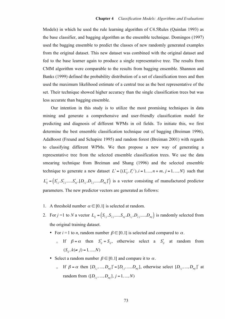
Chapter 4 Classification Models: Algorithms and Evaluations
73
Models) in which he used the rule learning algorithm of C4.5Rules (Quinlan 1993) as
the base classifier, and bagging algorithm as the ensemble technique. Domingos (1997)
used the bagging ensemble to predict the classes of new randomly generated examples
from the original dataset. This new dataset was combined with the original dataset and
fed to the base learner again to produce a single representative tree. The results from
CMM algorithm were comparable to the results from bagging ensemble. Shannon and
Banks (1999) defined the probability distribution of a set of classification trees and then
used the maximum likelihood estimate of a central tree as the best representative of the
set. Their technique showed higher accuracy than the single classification trees but was
less accurate than bagging ensemble.
Our intention in this study is to utilize the most promising techniques in data
mining and generate a comprehensive and user-friendly classification model for
predicting and diagnosis of different WPMs in oil fields. To initiate this, we first
determine the best ensemble classification technique out of bagging (Breiman 1996),
AdaBoost (Freund and Schapire 1995) and random forest (Breiman 2001) with regards
to classifying different WPMs. We then propose a new way of generating a
representative tree from the selected ensemble classification trees. We use the data
smearing technique from Breiman and Shang (1996) and the selected ensemble
technique to generate a new dataset
€
" L = {( " L ij , " I rj ), i =1, ..., n + m, j =1, ..., N} such that
€
" L ij = " S 1 j , " S 2 j ,..., " S nj , [D1 j ,D2 j ,...,Dmj " ] ( ) is a vector consisting of manufactured predictor
parameters. The new predictor vectors are generated as follows:
1. A threshold number
€
α ∈ [0,1] is selected at random.
2. For j =1 to N a vector
€
Lij = S1 j ,S2 j ,...,Snj ,D1 j ,D2 j ,...,Dmj( ) is randomly selected from
the original training dataset.
• For i =1 to n, random number
€
β ∈ [0,1] is selected and compared to
€
α .
o If
€
β =α then
€
" S ij = Sij , otherwise select a
€
" S ij at random from
€
(Sij , k(≠ j) =1, ..., N)
• Select a random number
€
β ∈ [0,1] and compare it to
€
α .
o If
€
β =α then
€
[D1 j , ...,Dmj " ] = [D1 j , ...,Dmj ], otherwise select
€
[D1 j , ...,Dmj " ] at
random from
€
([D1 j , ...,Dmj ], j =1, ..., N)

Chapter 4 Classification Models: Algorithms and Evaluations
74
This manufactured predictor vectors are then fed to the selected ensemble classifier
to predict a WPM type
€
( " I rj ) for each
€
" L ij . To generate the depictive tree we exploit two
approaches. Firstly, we follow Breiman’s approach and only use the new dataset
€
" L to
train the tree. Secondly, similar to the approach used by Domingos (1997), this new
manufactured dataset is combined with the original dataset
€
( " L + L) in an attempt to
retain the latent traits of the original problem. Contrary to what was suggested by
Breiman and Shang (1996) and Domingos (1997), instead of reapplying the base
classifier algorithm for generating the depictive tree, we use the more efficient
technique of LMT (Landwehr 2003). The procedure just described can be summarized
in a flowchart as presented in Figure 4.5.
4.4 Classification models performance measures
In this section, we briefly describe the measures used for evaluating the performance
of the developed classification models in discriminating WPMs. At first, we examine
the consistency and robustness of the models by means of a number of measures used
for evaluating ensemble classifiers. These measures are margin of prediction, proximity
measure, outliers and parameter importance.
Next, an independent validation dataset is used for evaluating the performance of the
models in predicting the WPMs of the cases in this dataset. At each stage of
implementing the classification models, the validation dataset, which contains N=238
cases of WPMs is incorporated in to the developed models to evaluate their
performance. The learnt patterns from the cases in the learning dataset are used to
evaluate the efficiency of the trained classification models in classifying each case into
one of Coning, Channelling, GravityDominated or the NoWater classes.
The performance of each implemented model is evaluated based on the overall
classification accuracy, sensitivity and Kappa value. We first use these measures to
compare ensemble classification models and select the best performing algorithm. We
then compare the two approaches used for generating the depictive tree using the
previously mentioned measures as well as a new measure called the area under ROC
curves (AUC) (Bradley 1997). Finally, we evaluate and compare the performance of the
selected born-again tree with the original best performing ensemble classification
algorithm.

Chapter 4 Classification Models: Algorithms and Evaluations
75
!
Training data
Bagging AdaBoost Random
forest
Select the best
ensemble classifier
Generate new data using smearing and the selected
ensemble classifier
Combine new and
original data
LMT
Test data
Database
Static reservoir characteristics from
each simulated case
Dynamic production data extracted from
WOR plots of each case
Evaluate final LMT models using the
test data
Figure 4.5 The flowchart of the procedure used for developing WPMs classification models

Chapter 4 Classification Models: Algorithms and Evaluations
76
4.4.1 Margin of predictions
Strength of the ensembles can be assessed using the margin of the predictions for
cases contained in the dataset. The margin of the jth case in the dataset is defined as the
difference between the average number of votes for the correct class and the maximum
average number of the votes for other classes. The margin of each case is used as a
measure of how confident the ensemble model is in classifying that case correctly. A
positive margin indicates that the majority of the trees in the ensemble voted for the
correct class, whereas, a negative margin indicates that the majority of the trees in the
ensemble could not correctly classify the case.
4.4.2 Proximity measure
The proximity measure provides a tool for understanding and visualizing the data
structure. Cases i and j are considered similar if they end up in the same terminal node
in each tree grown. The proximity measure is defined by the proportion of times that
cases i and j appear in the same terminal node across all trees grown in the ensemble.
Metric multi-dimensional scaling plots (MDS plots) are used for visualizing the
proximity measures between cases. These plots provide a more comprehensible picture
of the data structure. They can provide insights into possible clusters within classes and
closeness between cases. They can also help in finding hard or unusual cases in terms of
classification success.
4.4.3 Outliers
The outliers in the dataset are cases that do not properly fit into any of the known
classes. Using the concept of proximities, outliers can be defined as cases whose
proximities to other cases in the dataset are small. To calculate the outlier measure of
case j, in class r, firstly, the raw outlier measure for that case is calculated by dividing
the number of cases in that class by the average squared proximity of case j to the rest
of the cases in class r (Equation. 4.3). Within each class r, the median of all raw
measures and the absolute deviation for each case is calculated. Subtracting the median
from the raw measure of case j and dividing it by the absolute deviation gives the final
outlier measure for case j (Equation. 4.4). Generally cases with outlier measure of
greater than 10 are considered as outlier cases.
€
Outraw ( j) = jr proximity 2( j, r)∑ (4.3)

Chapter 4 Classification Models: Algorithms and Evaluations
77
€
Outnorm ( j) =Outraw ( j) −medianr[Outraw ( j)]Outraw ( j −medianr[Outraw ( j)])∑ jr
(4.4)
4.4.4 Parameter importance
The relevance of each predictor parameter in identifying the WPMs can be
approximated by a measure called the parameter importance. In tree-based ensemble
classification models, the mean decrease in accuracy and the mean decrease in gini
index (see section 4.3.1) are used to measure the quality of a split for each parameter in
a tree. Each tree in the ensemble is constructed using a bootstrap sample of about 2/3 of
the original data. The remaining cases referred to as out of bag (OOB) cases, are then
run down the tree to get a predicted classification. To measure the importance of
parameters, the difference between the mean squared error of the OOB data before and
after randomly permuting each predictor parameter is first calculated. The normalized
average of this number across all trees is defined as the importance of that parameter.
4.4.5 Classification accuracy
The efficiency of the implemented models in predicting the type of the WPM of the
cases in the validating data is evaluated using the percentage of correctly classified
cases. Classification accuracy (or its complement, misclassification error) is used
commonly for evaluating classification models. A confusion matrix, similar to table 4.3,
can be used to calculate the prediction accuracy. Confusion matrix is a matrix whose
rows represent the true classifications and columns represent the classifications made by
the algorithm.
Table 4.3 The confusion matrix corresponding to classification of WPMs
Predicted
Channelling Coning Gravity Dominated NoWater
Act
ual Channelling P1 P2 P3 P4
Coning P5 P6 P7 P8
GravityDominated P9 P10 P11 P12
NoWater P13 P14 P15 P16

Chapter 4 Classification Models: Algorithms and Evaluations
78
In the confusion matrix shown in table 4.3, classification accuracy is calculated by:
€
Accuracy =P1 + P6 + P11 + P16
Pii=1
16
∑ (4.3)
4.4.6 Sensitivity
Another measure used to evaluate the performance of the classification models is
sensitivity. The sensitivity of a model is defined by the proportion of the cases correctly
identified as their actual classes. Using the confusion matrix in table 4.2, the sensitivity
of the models with respect to each class of WPMs can be calculated as:
€
SensitivityChannelling =P1
P1 + P2 + P3 + P4 (4.4)
€
SensitivityConing =P5
P5 + P6 + P7 + P8 (4.5)
€
SensitivityGravityDomiated =P9
P9 + P10 + P11 + P12 (4.6)
€
SensitivityNoWater =P13
P13 + P14 + P15 + P16 (4.7)
4.4.7 Kappa coefficient
Despite the wide use of classification accuracy measure, it is not a perfect measure.
It has been demonstrated by Arie (2007) that a classifier’s predictions may be due to
mere chance. He states that classifiers’ accuracy should be compared after
compensating for random hits and one way to do this is the use of Kappa value (Cohen
1960). Kappa measures the agreement between two categorical parameters while taking
in to account those successfully classified cases that might be attributed to chance alone.
Using a confusion matrix and calculating Po (observed agreement) and Pc (chance
agreement), the Kappa value can be calculated as follows:
€
K =Po − Pc1− Pc
(4.8)
Kappa coefficient can range from 1 (perfect agreement) to -1 (complete disagreement).
A kappa value of zero indicates no agreement above that expected by chance.

Chapter 4 Classification Models: Algorithms and Evaluations
79
4.4.8 Area under ROC curves (AUC)
The ROC (receiver operating characteristics) curve is a graphical plot of true
positives (sensitivity) against false positives (1 − specificity). Each point on the ROC
curve represents a prediction result or one instance of a confusion matrix corresponding
to a particular decision threshold. The accuracy of a test depends on how well the test
separates the cases being tested into one of the problem types in question. Accuracy of
the test can be shown using the area under the ROC curve (AUC) (Bradley 1997),
which represents a quantitative summary measure of the curve. Larger AUC values
correspond to more accurate tests. An area of 1 represents a perfect test and an area of
0.5 represents a poor diagnostic test.
4.5 Summary
In this chapter, we explained in details the procedure for implementing
classification models for diagnosing different WPMs. For this purpose, the simulated
reservoir models described in chapter 3 were used to construct a learning dataset on
which the classification models are trained and existing patterns in the data are
recognized. We explained how we considered the WPMs classification problem in three
different scenarios and integrated reservoir characteristics parameters with the RFWOR
parameters extracted from WOR-RF plots introduced in chapter 3. Next, we briefly
introduced the classification algorithms we intend to use in this study and introduced the
anticipated classification process. The measures that will be used later for evaluating the
implemented classification models were also explained. In the next chapter, we present
and compare the results from each stage of implementing the classification models. We
first use the evaluation measures to compare ensemble classification models and select
the best performing algorithm. The two approaches used for generating the born-again
tree are then compared and finally, the performance of the selected born-again tree with
the original best performing ensemble classification algorithm are evaluated and
compared.

Chapter 5 Results and Discussions
80
Results and Discussions
In chapter 3, we explained in detail how a wide range of simulated reservoir models
were generated to represent various water production mechanisms (WPM) in oil fields.
These simulated reservoir models cover a broad range of oil fields characteristic
encountering excess water production problems. In chapter 4, we presented details of
building the database from these models, where each row represents one case of WPM
and columns represent corresponding parameters (static and dynamic) values and
classification index for WPM. Chapter 4 also described the algorithms for constructing
the statistical classification model based on classification trees.
In this chapter, we present the results of ensemble classification techniques used for
identifying different WPMs. Two thirds of the cases in the generated database are used
for constructing and training the ensemble models. The remaining cases are used for
evaluating and comparing the efficiency of the developed models. The random
sampling process is repeated five times and the average of the results is presented where
appropriate. The models are developed for three scenarios namely pre-production, post-
production with static parameters and post-production without static parameters.
Section 5.1 focuses on the results obtained from the random forest (RanFo) models.
Section 5.2 presents a comparison between RanFo models and two other ensemble
classification techniques investigated in this study, namely bagging and AdaBoost
algorithms. Next, in section 5.3, we move on to investigating the efficiency of a
depictive tree as a single representative of the RanFo models. We propose a new way of
developing the depictive tree using logistic model trees (LMT) algorithm (Landwehr
2003) in two approaches. Firstly, we generate a new dataset using the original RanFo
models based on the methodology suggested by Breiman (2001) and construct the
depictive tree on this new dataset. Secondly, we combine the original database with this
newly generated dataset and construct another depictive tree. The performances of these
depictive trees are first compared together and the best performing depictive tree is then
evaluated against the original ensemble RanFo models in section 5.4. A thorough
discussion on the results presented is given in section 5.5. Ultimately, in section 5.6, we
5

Chapter 5 Results and Discussions
81
conclude through our results that the depictive tree trained on the combined datasets
offers the most efficient classification model with high accuracy rates of at least 90%,
93% and 82% for the three scenarios discussed in chapter 4, respectively.
5.1 Evaluation of the random forest models
The first of the classification models is developed by using RanFo method on the
learning data set and its accuracy is evaluated on the validation set. Essentially, the
RanFo algorithm grows an ensemble of trees using the learning data and takes the
majority vote from these trees to predict the type of the WPM. Figure 5.1 illustrates the
structure of a tree grown in the RanFo ensemble. For demonstration purpose, only a
section of the whole tree is shown in this figure. The full RanFo model comprises of
several trees and is computationally easy to implement for prediction purposes.
As was explained in chapter 4, we consider three different scenarios for developing
models. The model in the first scenario contains only the static reservoir characteristics
in the pre-water-production state. The second scenario concerns the post-water-
production phase and includes a group of sequential models (Models#(1-14)), which
contain both the reservoir characteristics and dynamic production data parameters
extracted from plots of water/oil ratio (WOR) versus recovery factor (RFWOR). The third
scenario again includes a group of sequential models (Models#(1*-14*)) concerning the
post-water-production phase except that these models are based on the dynamic
production data alone without any reservoir characteristics. In the following
subsections, we provide some general overviews of the model appraisal in classification
task, and present the results of evaluating the performance of the implemented models
in classifying the cases in a validation dataset.
5.1.1 Model appraisal
Margin of predictions
The sensitivity of the RanFo model can be expressed by a measure called the margin
of the predictions (see section 4.4.1). As the majority vote is regarded as the final
prediction outcome, the margin of error indicates the sensitivity of the ensemble in the
classification. A positive margin indicates that the majority of the trees in the ensemble
voted for the correct class, whereas, a negative margin indicates that the majority of the
trees in the ensemble could not correctly classify the case.

Chapter 5 Results and Discussions
82
Left node Right node Split parameter Split point Prediction
2 3 PP 17.5 – 4 5 RFWOR0.1 0.062 – 6 7 RFWOR0.1 0.006 –
Terminal Terminal – – Coning 8 9 IOFR 0.0014 –
Terminal Terminal – – NoWater 10 11 RFWOR0.5 0.222 –
Terminal Terminal – – Channelling 12 13 IOFR 0.002 – 14 15 DA Medium – 16 17 AQWOV 308 –
Terminal Terminal – – Coning Terminal Terminal – – Channelling
18 19 IOFR 0.0006 – Terminal Terminal – – Coning
20 21 RFWOR0.5 0.345 – 22 23 RFWOR0.1 0.275 – 24 25 RFWOR0.5 0.123 – 26 27 PP 31.5 –
Terminal Terminal – – Channelling 28 29 WET Intermediate wet – 30 31 AQWOV 533 – . . . . . . . . . . . . . . .
Figure 5.1 Section of a tree from the RanFo ensemble models; at each node the cases with split
parameter values less than the splitting point go to the left daughter node and the rest go to the right daughter node (PP, IOFR, DA, AQWOV and WET refer to plateau period, initial oil flow rate, drainage area, aquifer strength and wettability, respectively)
For demonstration purpose, one model from each scenario is selected (Model#0,
Model#1 and Model#1*) and the margins of the learning cases obtained from these
models are shown in Figure 5.2. This figure shows that Model#1 gives the highest
margins for the cases with only a limited number of cases with negative margins,
especially in the GravityDominated group. This translates to the higher strength of this
model in correctly classifying the WPM cases. This model is armed with a combination
of reservoir characteristics and dynamic production data, which enable the model to
identify a more robust pattern of interaction between parameters causing a specific type
of WPM.
!
8 9 10 11
!
PP <17.5
!
RFWOR 0.5
< 0.222 !
RFWOR 0.1
< 0.006
2 3
!
IOFR < 0.0014
4 5 6 7
!
RFWOR 0.1
< 0.062
NoWater Coning

Chapter 5 Results and Discussions
83
It is obvious from the figure that Model#1* is the least confident in classifying the
GravityDominated cases. Comparing the case margins in each class category reveals
that the NoWater cases have the highest chance of being correctly classified using the
post-water-production models, followed by the Coning cases. Model#0 and Model#1
perform comparably with respect to classifying the Channelling cases.
Figure 5.2 Margins of predictions for cases by example RanFo models from pre and post-water-
production
Proximity measure
The proximity measure is the proportion of times the two cases say (i and j) appear
in the same terminal node, hence were predicted to have same WPM, across the trees in
the ensemble. In general high value of proximity measure will imply cases have similar
structure. The hidden pattern in the dataset can be visualized and investigated by
calculating the Eigen vectors of the dissimilarity matrix (1-proximity) and projecting it
Model#0
Model#1
Model#1*

Chapter 5 Results and Discussions
84
on multi-dimensional scaling plots (MDS plots) (Section 4.4.2). These plots provide
insights into possible clusters within classes and closeness between cases. They can also
help in finding hard or unusual cases in terms of classification success.
Usefulness of proximity measure can be evaluated from two points of view. One is
to investigate the ability of the model to clearly identify the pre-specified structure of
the data imposed by the classes, which in this study are different types of WPMs. The
other is the ability of the model to discover structures in the data based on unknown
internal criteria, which may not necessarily comply with the pre-specified classes.
From WPM classification point of view and with regards to excess water
production problems, this aspect of proximity measure can be particularly useful in
water control and selection of the effective treatment technology. Water control and
water shutoff treatment is a complex process, which usually involves uncertainties even
if the exact type of the WPM is known. Many unknown or unforeseen parameters could
influence the success of the treatment methodology. One helpful approach advocated
from the proximity measure could be to use similar treatment options for cases within a
cluster or reuse of the experience from cases of WPM with known successful treatment
history within the cluster. New situation-specific knowledge can be derived from a
cluster containing previously solved problems, which could help in designing the water
shutoff treatment for a new case.
The MDS plot of proximity measure from Model#0 (Figure 5.3.a) shows that this
model lacks the ability to form a distinctive cluster for the Coning cases based on
reservoir parameters alone. Clusters for other class categories are nearly formed
although there is an overlap between them in this dimension. The MDS plot of
Model#1, (Figure 5.3.b) displays a favorable clustering tendency. Cases in the Coning
and Channelling classes are more compact and only a few of the cases are positioned far
from their actual clusters. Cases in the GravityDominated and the NoWater classes are
well grouped together, while an overlap is still observed in this dimension.
An interesting separation in Coning cases can be seen in the MDS plot of proximity
measure from Model#1* shown in Figure 5.3.c. This separation could be an example of
what was discussed before regarding the selection of the treatment methodology. A
Coning problem in one cluster might require a different approach for water control than
a Coning problem in the other cluster. Other classes are perfectly separable with only a
few cases positioned out of any particular clusters.

Chapter 5 Results and Discussions
85
-0.2 -0.1 0.0 0.1 0.2 0.3 0.4
-0.4
-0.2
0.0
0.2
1st scaling coordinate
2n
d s
ca
ling
co
ord
ina
te
-0.4 -0.2 0.0 0.2 0.4
-0.4
-0.2
0.0
0.2
0.4
1st scaling coordinate
-0.2 0.0 0.2 0.4
-0.2
0.0
0.1
0.2
0.3
0.4
1st scaling coordinate
ChannellingConingGravityDominatedNoWater
Figure 5.3 Multi-dimensional scaling plot of proximity measure from (a) Mode#0, (b) Model#1 and (c)
Model#1*
Outliers
The outliers in the dataset are cases that do not comply with the general behavior of
any of the known classes. Using the concept of proximities, outliers can be defined as
cases whose proximities to other cases in the dataset are small and hence do not fit in to
the formed clusters (see Section 4.4.3). Nevertheless, the outlier cases could reveal
important information. In this study, detected outliers could lead to identification of
unique WPMs. These outlier cases might at first appear similar to the common
problems but could in fact be very different in nature and hence require specific
treatment techniques. An outlier case can also be a showcase of extreme conditions of
the common WPMs, which again calls for specifically tailored treatments. In either
situation, further studies and more detailed examination of the outlier cases are required
to determine the remedial actions to be taken. Detailed investigation on the outlier
cases is beyond the scope of this study, however, opens a very interesting road for
future developments.
In this study, we follow the commonly used outlier measure threshold of 10 (see
section 4.4.3) for detecting the outliers. Nevertheless, further examinations of the outlier
cases might lead to a different threshold specific to WPM studies. Based on this
threshold, it is obvious from Figure 5.4 that in all scenarios, only a few of the Coning
cases in our dataset are picked up as outliers. These cases were also clearly singled out
in the MDS plots of proximity shown in the last section.
Variable importance
Evaluating and comparing the predictor variables by just visually assessing the
large number of trees in a RanFo model is impossible. However, it is possible to define
which predictor variables play the most important role in classification by calculating
the mean decrease in accuracy. When the number of predictor variables is large, the
(a) (b) (c)

Chapter 5 Results and Discussions
86
variable importance can be useful in reducing the dimension of the dataset by selecting
the most important variables. The variable importance measure can also give an
informative insight into the discriminating role of the selected predictor variables. This
determines the minimum required information for development of a successful
classification model. Figures 5.5 and 5.6 show the variable importance based on mean
decrease in accuracy measure for Model#0 and Model#1.
Figure 5.4 Outlier cases identified by example RanFo models in pre and post-water-production
scenarios
Based on this measure, in both scenarios, wettability (WET) does not have a
discriminating role in terms of predicting the type of the WPMs, even though it has
significant effects on the amount of the produced water. In addition to the importance of
Model#0
Model#1
Model#1*

Chapter 5 Results and Discussions
87
variables in general classification, the importance of variables with respect to each class
is also shown. In Model#0, plateau period for the initial oil flow rate (PP) is the most
dominate predictor in general classification followed by aquifer volume (AQWOV).
Looking at the class specific importance plot, it is revealed that as expected in the
GravityDominated cases, the vertical to horizontal permeability (Kv/Kh) plays an
important role in characterizing this type of problem, while in NoWater cases the
AQWOV plays the critical role.
Figure 5.5 Variable importance plots based on Model#0; plots (a–d) show the importance of the
parameters with respect to each WPM and plot (e) shows the importance of the parameters in overall classification
In Model#1, however, we can see a change in the importance rankings of the
reservoir characteristics in identifying each class. Comparing the plots of the two
scenarios reveals that once water breaks into the well, the extracted WOR parameters
are more important predictors than the reservoir characteristic parameters. This once
e) Overall importance d) NoWater
c) GravityDominated b) Coning a) Channelling
IOFR
IOFR IOFR
IOFR
IOFR

Chapter 5 Results and Discussions
88
again emphasizes that production data are essential for accurate prediction of the WPMs
in petroleum reservoirs. The effect of each parameter on the WPMs can be more
investigated using the partial dependency plots explained in the next section.
Figure 5.6 Variable importance plots based on Model#1, plots (a–d) show the importance of the
parameters with respect to each WPM and plot (e) shows the importance of the parameters in overall classification
Partial dependency
In addition to understanding the importance of each predictor in classification, it is
also desirable to know how each predictor affects the response. In current context this
would imply understanding the sensitivity of a parameter in affecting the likelihood of
the WPM. Such sensitivity is examined by constructing the so-called partial
dependence plots (Hastie et al. 2001). However, these plots need to be interpreted with
caution as these correspond to the one-factor-at-a-time (OFAT) experiments. That is,
these plots do not account for the complex interaction between predictor parameters.
a) Channelling b) Coning c) GravityDominated
d) NoWater e) Overall importance
IOFR IOFR
IOFR
IOFR IOFR

Chapter 5 Results and Discussions
89
Partial dependence plots show this relationship with respect to the class labels of the
response parameter, which in our study is WPM. Positive values indicate an increased
likelihood of a specific WPM occurrence and negative values indicate a decreased
likelihood. The horizontal axis represents the range or levels of the predictor
parameters. Figures 5.7 and 5.8 display the partial dependence plots for predictor
parameters in Model#1 with respect to the Channelling and Coning problems
respectively.
Figure 5.7 Partial dependence plots of the predictor parameters on Channelling problem based on
Model#1
IOFR

Chapter 5 Results and Discussions
90
Figure 5.8 Partial dependence plots of the predictor parameters on Coning problem based on Model#1
Figure 5.7 suggests that Channelling is less likely to happen in reservoirs with high
degree of crossflow between layers (Kv/Kh=0.1) and intermediate level of API. High
degrees of IOFR and AQWOV are associated with less likelihood of the problem being
Channelling. Whereas, high PP and WIR values mean more chances of causing a
Channeling problem. The WIR partial dependency plot conforms the fact stated in the
literature that increased rate of water injection results in an increase chance of a
Channelling problem. While a vary large drainage area (DA > 150 acres) has a positive
IOFR

Chapter 5 Results and Discussions
91
affect on causing this type of problem, smaller ranges of drainage area do not seem to
be important. We observe an almost linear increased chance of Channelling problem for
dynamic RFWOR0.1 and RFWOR0.5 between 0.05–0.25 and 0.1–0.3 respectively, after
which, the likelihood of Channelling problem remains constant. This means that the
high initial rate of excess water production could be a strong indication of a
Channelling problem.
From Figure 5.8, we can conclude that reservoirs with lighter oil and vertical
equilibrium permeability are more expected to experience a Coning problem. AQWOV,
as is expected, has a direct effect on the Coning problem. It seems that large values of
IOPVFR do not have any effect on forming this problem while large PP values decrease
the chance of it happening. Opposite to the Channelling mechanism, drainage areas of
less than 150 acres seem to be associated with Coning problem occurring. Interestingly,
the partial plots of the RFWOR parameters coincide with the common behaviour of a
water cone forming. The water breakthrough into the well starts with a small amount
and gradually increases as the water cone moves closer to the vicinity of the well. This
is reflected in the partial plots by showing that the small amounts of initial water
production rate is related to a Coning problem whereas, higher amounts of initial excess
water could be an indication of other problem types.
5.1.2 Performance accuracy
The RanFo model performance is assessed based on the percentage of correctly
classified cases, which is calculated by dividing the total number of correctly classified
cases by the number of cases tested in each model. To ensure consistency of the results
obtained by the classifiers, we repeated each classification algorithm five times and
present the average obtained from each algorithm. Figure 5.9 presents the total average
accuracy rates for all the models in pre and post-water-production scenarios. This figure
shows that the overall performance of the models, which use both reservoir parameters
and RFWOR data, is superior to that of the models, which only use either one of these
groups. Nevertheless, the performance of Model#0, which only uses the reservoir
parameters, is still very impressive with 91% accuracy. The accuracy of the
Models#(1-14) in the post-water-production scenario reaches a maximum of 96%, with
accuracy ranging between 92% and 96%. A drop in accuracy for Models#(1*-14*) can
be observed, however, accuracy values stay fairly constant within a range of 85%–87%.
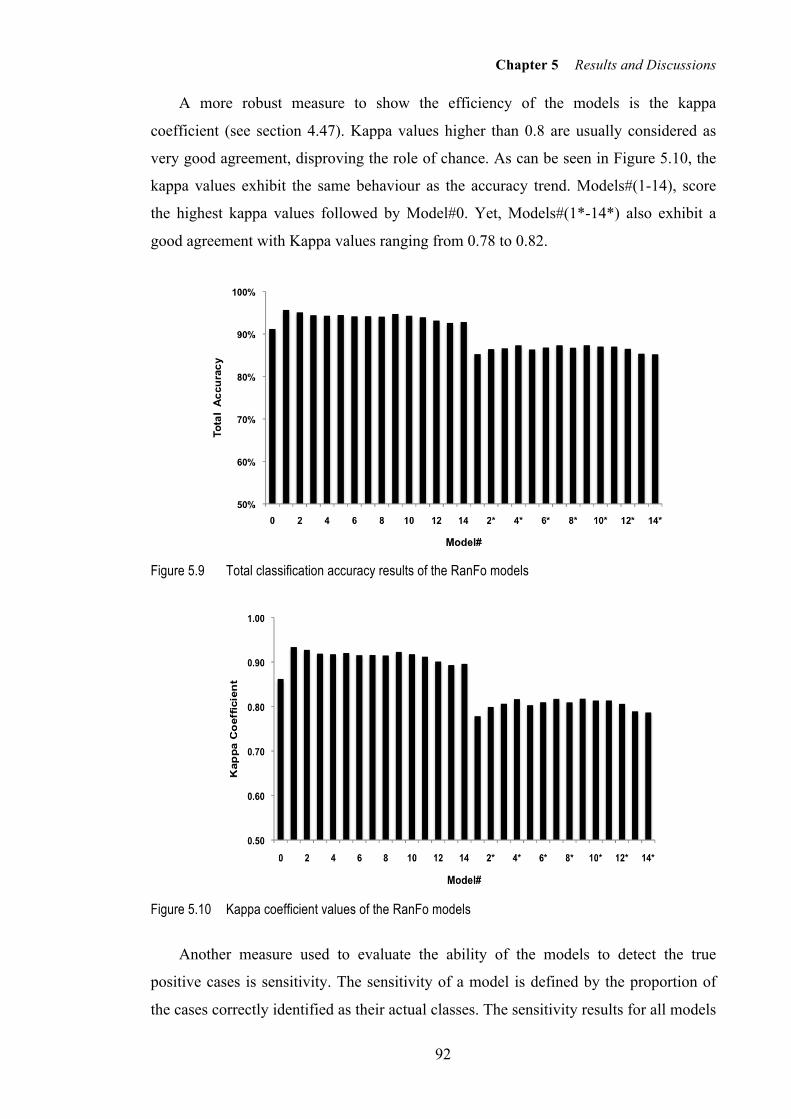
Chapter 5 Results and Discussions
92
A more robust measure to show the efficiency of the models is the kappa
coefficient (see section 4.47). Kappa values higher than 0.8 are usually considered as
very good agreement, disproving the role of chance. As can be seen in Figure 5.10, the
kappa values exhibit the same behaviour as the accuracy trend. Models#(1-14), score
the highest kappa values followed by Model#0. Yet, Models#(1*-14*) also exhibit a
good agreement with Kappa values ranging from 0.78 to 0.82.
Figure 5.9 Total classification accuracy results of the RanFo models
Figure 5.10 Kappa coefficient values of the RanFo models
Another measure used to evaluate the ability of the models to detect the true
positive cases is sensitivity. The sensitivity of a model is defined by the proportion of
the cases correctly identified as their actual classes. The sensitivity results for all models

Chapter 5 Results and Discussions
93
are presented in Figure 5.11. This figure shows that across all models, the
GravityDominated cases get the least favourable classification accuracy compared to the
other WPMs. While all dynamic models score a perfect 100% accuracy rate in
identifying the NoWater cases, Model#0 fails to do so and gains an accuracy rate of
84%. The accuracy rate of identifying the Channelling cases remains almost unchanged
between Model#0 and Models#(1-14). An improvement in classifying the Coning cases
is noticeable after the introduction of the RFWOR data in the models. However, it starts
to decline towards the higher numbered models corresponding to high amounts of water
production and continues to decrease in Models#(1*-14*).
Figure 5.11 Sensitivity results of the RanFo models with respect to water production mechanisms
5.1.3 Consistent classification
The consistency of the RanFo models in allocating each validating case to one of
the classification categories can be further explored in a very interesting display of the
predicted classification that each case gets from sequential implementation of Model#0
to Model#14. Each model in increasing index indicates the progression of well
depletion. This plot is specifically designed for this study and is not available from R
software. Figure 5.12 shows the associated votes for each case with regards to the
model used in a colour-coded bar-plot. Each column in the bar plot corresponds to a
case from the validating dataset. The rows correspond to the predicted class for each
case by each model.

Chapter 5 Results and Discussions
94
Since the Models#(1-14) are developed based on sequential addition of production
data, the presented sequential classes overview can help in assessing the consistency of
the models at each stage in predicting the WPM. By assessing the models in sequence,
cases that have been consistently misclassified can be identified and further examined to
reveal any possible mistakes or abnormalities in those specific WPM cases.
Additionally, it is important to bear in mind that if a WPM is wrongly diagnosed, the
results from the applied treatment methodology for that specific misdiagnosed problem
type are not reversible and might even further complicate the field conditions. As a
result, it is vital to have a tool for identifying the misclassified cases and the
corresponding models in order to highlight the situations in which the models perform
poorly.
Figure 5.12 highlights the misclassified cases by Model#0 and Models#(1-14). It is
clear that number of the misclassified cases in Model#0 is significantly higher than that
of Models#(1-14). Especially, when the amount of the produced water is not large, the
models perform very well and the number of misclassified cases is limited.
0
1
2
3
4
5
6
7
8
9
10
11
12
13
14
15
16
17
18
19
1 13 26 36 49 59 11 82 114 150 81 134 178 120 71 106 144 174 146 191 201 211 221 231
Mo
del #
Case #
!!Actual classes of the test cases
Pre
dic
ted
cla
sses u
sin
g M
od
el#
(1-1
4)
!!!Predicted classes using Model#0
14
13
12
11
10
9
8
7
6
5
4
3
2
1
!"!!!!!!!!"#!!!!!!!!$#!!!!!!!%#!!!!!!!&#!!!!!!!'#!!!!!!!!(#!!!!!!!)#!!!!!!!!*#!!!!!!!+#!!!!!!!"##!!!!!!!""#!!!!!!!"$#!!!!!!!"%#!!!!!!!"&#!!!!!!!"'#!!!!!!!"(#!!!!!!")#!!!!!!"*#!!!!!!"+#!!!!!!!$##!!!!!!!$"#!!!!!!!$$#!!!!!!!$%#!!
Channelling Coning GravityDominated NoWater Cases not reaching the threshold Figure 5.12 The sequential classification votes allocated to each case using RanFo models in
pre and post-water-production scenarios

Chapter 5 Results and Discussions
95
5.2 Comparison of random forest algorithm to other ensemble classification techniques
In this section, we present the results of two other commonly used ensemble
classifiers, namely bagging and AdaBoost techniques, and compare their performance
with the RanFo models discussed so far. Similar to the RanFo models, and to ensure
consistency of the results, we repeated each classification algorithm five times and
present the average results obtained from each algorithm. For comparison, we present
the results of the bagging and AdaBoost models along with the results of the RanFo
models together with the p-values for statistically comparing the models in table 5.1.
In bagging models, introducing the RFWOR parameters in the model, at first
(Model#1), results in a slight improvement in total classification accuracy compared to
Model#0. However, no further improvements higher than 93% accuracy can be
observed in subsequent models. The kappa values exhibit almost the same behaviour
with 0.04 improvement in Model#1 and 0.01 further improvements for the consecutive
models. The accuracy rates obtained from Models#(1*-14*) in bagging and RanFo
algorithms are comparable with bagging models being slightly lower. Again, the Kappa
values follow a similar behaviour and we can observe 2 to 3 units decrease in bagging
models.
Contrary to RanFo and bagging algorithms, the classification accuracy rates in
AdaBoost models for all scenarios are relatively low. The associated kappa values also
start at a low level and no real improvements are observed with the introduction of
RFWOR parameters in the consecutive models.
The P-value of less than 0.05 for all models in Table 5.1, indicates that we have
sufficient evidence to conclude that the accuracy rates across all the methods is not
same. Further testing reveals that, with reference to accuracy, the performance of the
RanFo and bagging models are comparable and higher than AdaBoost models. Similar
conclusions can be drawn for the Kappa values. In conclusion, the overall performance
of RanFo and bagging models with respect to both total accuracy and Kappa values are
comparable and significantly higher than AdaBoost models. Although, RanFo and
bagging models perform comparably, because RanFo algorithm is usually more robust
to parameter sensitivity than other ensemble techniques, we choose this algorithm for
further investigations. In the next section, we demonstrate how the developed RanFo

Chapter 5 Results and Discussions
96
models can be further improved to provide a more perceivable display of the tree
structure. Table 5.1 Performance comparison between random forest, bagging and AdaBoost classification algorithms based on total accuracy and Kappa. The last column presents the P-value for comparing the accuracy across RanFo, bagging and AdaBoost methods using a chi-square test
RanFo Bagging AdaBoost P-value
Model# Accuracy Kappa Accuracy Kappa Accuracy Kappa 0 91% 0.86 90% 0.85 66% 0.36 < 0.00001 1 96% 0.93 93% 0.89 68% 0.49 < 0.00001 2 95% 0.93 93% 0.89 78% 0.68 < 0.00001 3 94% 0.92 91% 0.87 69% 0.54 < 0.00001 4 94% 0.92 92% 0.88 69% 0.54 < 0.00001 5 94% 0.92 91% 0.87 66% 0.49 < 0.00001 6 94% 0.91 91% 0.87 66% 0.49 < 0.00001 7 94% 0.92 93% 0.90 67% 0.50 < 0.00001 8 94% 0.91 93% 0.90 67% 0.50 < 0.00001 9 95% 0.92 93% 0.90 67% 0.50 < 0.00001
10 94% 0.92 92% 0.89 63% 0.44 < 0.00001 11 94% 0.91 92% 0.89 63% 0.44 < 0.00001 12 93% 0.90 91% 0.88 61% 0.40 < 0.00001 13 92% 0.89 90% 0.86 62% 0.42 < 0.00001 14 93% 0.89 92% 0.89 65% 0.44 < 0.00001 1* 85% 0.78 85% 0.77 68% 0.49 0.00001 2* 86% 0.80 85% 0.77 78% 0.68 0.07 3* 87% 0.81 85% 0.78 69% 0.54 0.00001 4* 87% 0.82 84% 0.77 69% 0.54 < 0.00001 5* 86% 0.80 85% 0.78 66% 0.49 < 0.00001 6* 87% 0.81 86% 0.79 66% 0.49 < 0.00001 7* 87% 0.82 85% 0.78 67% 0.50 < 0.00001 8* 87% 0.81 85% 0.78 67% 0.50 < 0.00001 9* 87% 0.82 85% 0.78 67% 0.50 < 0.00001
10* 87% 0.81 86% 0.79 63% 0.44 < 0.00001 11* 87% 0.81 85% 0.78 63% 0.44 < 0.00001 12* 86% 0.80 85% 0.78 61% 0.40 < 0.00001 13* 85% 0.79 84% 0.77 62% 0.42 < 0.00001 14* 85% 0.79 84% 0.76 65% 0.44 < 0.00001
5.3 Evaluation of the depictive trees
In the last section, we demonstrated the usefulness of RanFo algorithm in
identifying various WPMs. Despite the many advantages that these models provide for
the user, one major drawback of ensemble classifiers such as RanFo is the lack of an
intuitively simple and easy to understand structure.
To alleviate this problem, we used a depictive tree to produce a single and
comprehendible tree for each ensemble RanFo model. The algorithm for constructing
the depictive tree was explained in details in the last chapter (see section 4.3.4). We
establish through our results that the usually complex results obtained from aggregation
of trees in RanFo algorithm can be represented through a simple and more
understandable depictive tree structure with comparable or even superior performance.

Chapter 5 Results and Discussions
97
Figure 5.13 shows the structure of one of the depictive trees developed. The associated
logistic regression equations for each terminal node are shown in Table 5.2.
!
LM-1
LM-2
RFWOR0.5 ! 0
RFWOR0.1 ! 0.16
AQWOV ! 0
LM-3
LM-4
Figure 5.13 The structure of a developed depictive tree model
5.3.1 Evaluation and comparison of the depictive trees using new and combined
datasets
In this section, we first present the results obtained from the depictive trees trained
on new (depictive-new henceforth) and combined data (depictive-combined henceforth)
and investigate the competency of the latter approach. Once the efficiency of this
method is established, we move on to evaluating the performance of this method
compared to the original RanFo models.
Table 5.3 displays a comparison of the accuracy and Kappa values for
depictive-new and depictive-combined models. As was expected, we observe increased
accuracy and Kappa values in Model#0 and Models#(1-14) for the depictive-combined
trees compared to the depictive-new trees. For lower values of RFWOR in
Models#(1*-14*) both approach produce similar results. However, as more RFWOR are
included in the models, the depictive-combined trees produce slightly higher accuracy.
The P-value of more than 0.05 for all models in Table 5.3, indicates that we have
insufficient evidence to conclude that the accuracy rates across the two methods are
different. The results in this instance for the two models are comparable due to discrete
nature of many parameters and their re-sampling in the process of data smearing.
The effect of combining the new data with the original data to train the depictive
trees can be further investigated using the sensitivity of the trained models in correctly
classifying each WPM. Table 5.4 shows the sensitivity of the depictive-new and
depictive-combined models in identifying correct cases in each problem category.

Chapter 5 Results and Discussions
98
Table 5.2 The logistic regression equations for each terminal node in the developed depictive tree shown in Figure 5.13
Class Channelling Class Coning Class GravityDominated Class NoWater
LM-1
-68.45 + [Kv.Kh] x -0.33 + [API] x -0.12 + [WET=IntermedWet] x 1.98 + [WET=OilWet] x 0.08 + [IOPVFR] x 488.67 + [PP] x 0 + [DA=Large] x -1.98 + [DA=Medium] x -0.14 + [DA=VeryLarge] x 1.58 + [AQWOV] x 0 + [WIR] x 0 + [WOR0.1] x 7.59 + [WOR0.5] x 6.52 + [WOR2] x 1.29
-68.16 + [API] x 0.13 + [WET=IntermedWet] x -4.5 + [WET=OilWet] x -0.06 + [WET=WaterWet] x 0.28 + [IOPVFR] x -206.42 + [PP] x -0.01 + [DA=Large] x 0.18 + [DA=Medium] x -1.16 + [DA=Small] x 0.34 + [AQWOV] x 0 + [WIR] x 0 + [WOR0.1] x -38.64 + [WOR2] x 1.27
-81.08 + [Kv.Kh] x 13.86 + [API] x -0.11 + [WET=IntermedWet] x 0.2 + [WET=OilWet] x 0.59 + [WET=WaterWet] x -1.01 + [IOPVFR] x -1307.57 + [PP] x 0 + [DA=Medium] x 0.11 + [DA=Small] x -1.01 + [DA=VeryLarge] x -2.51 + [AQWOV] x 0 + [WIR] x 0 + [WOR0.5] x 14.96 + [WOR1] x 2.36
167.06 + [API] x -0.05 + [WET=IntermediateWet] x -0.01 + [WET=OilWet] x 0.03 + [WOR0.1] x -3268.13 + [WOR0.5] x -64028.51 + [WOR2] x -74.99
LM-2
2.92 + [Kv.Kh] x -0.33 + [API] x -0.24 + [WET=IntermedWet] x -0.1 + [WET=OilWet] x 0.15 + [IOPVFR] x 356.84 + [PP] x 0 + [DA=Large] x -1.84 + [DA=Medium] x -0.14 + [DA=Small] x -0.06 + [DA=VeryLarge] x 2.03 + [AQWOV] x 0 + [WIR] x 0 + [WOR0.1] x 15.67 + [WOR0.5] x 8.47 + [WOR1] x -5.88 + [WOR2] x 6.54
0.5 + [Kv.Kh] x -0.08 + [API] x 0.28 + [WET=IntermedWet] x 0.8 + [WET=OilWet] x -1.37 + [WET=WaterWet] x -0.04 + [IOPVFR] x 98.94 + [PP] x 0 + [DA=Large] x 1.11 + [DA=Medium] x -1.21 + [DA=Small] x 1.34 + [AQWOV] x 0 + [WIR] x 0 + [WOR0.1] x -52.84 + [WOR0.5] x -7.51 + [WOR2] x 1.61
-28.5 + [Kv.Kh] x 16.39 + [API] x -0.12 + [WET=OilWet] x 3.8 + [WET=WaterWet] x -1.2 + [IOPVFR] x -3838.85 + [PP] x 0.02 + [DA=Medium] x 9.91 + [DA=Small] x -1.01 + [DA=VeryLarge] x -4.04 + [AQWOV] x -0.01 + [WIR] x 0 + [WOR0.5] x 18.4 + [WOR1] x 33.61 + [WOR2] x -32.06
52.15 + [WOR0.1] x -3315.49 + [WOR0.5] x -64028.51 + [WOR2] x -74.99
LM-3
8.58 + [Kv.Kh] x -0.87 + [API] x -0.68 + [WET=IntermedWet] x -0.89 + [WET=OilWet] x 0.76 + [WET=WaterWet] x -0.39 + [IOPVFR] x 503.26 + [PP] x 0 + [DA=Large] x -2.65 + [DA=Medium] x 0.14 + [DA=Small] x -1.71 + [DA=VeryLarge] x 3.14 + [AQWOV] x 0 + [WIR] x 0 + [WOR0.1] x 63.24 + [WOR0.5] x 2.99 + [WOR1] x -8.47 + [WOR2] x 9.76
-5.41 + [Kv.Kh] x 0.84 + [API] x 0.74 + [WET=IntermedWet] x 1.6 + [WET=OilWet] x -2.4 + [WET=WaterWet] x 0.35 + [IOPVFR] x -47.48 + [PP] x 0 + [DA=Large] x 1.93 + [DA=Medium] x -1.48 + [DA=Small] x 2.98 + [DA=VeryLarge] x -0.65 + [AQWOV] x 0 + [WIR] x 0 + [WOR0.1] x -99.6 + [WOR0.5] x -2.03 + [WOR1] x 2.59 + [WOR2] x -1.61
-77.26 + [Kv.Kh] x 16.39 + [API] x -0.12 + [WET=OilWet] x 3.8 + [WET=WaterWet] x -1.2 + [IOPVFR] x -3838.85 + [PP] x 0.02 + [DA=Medium] x 9.91 + [DA=Small] x -1.01 + [DA=VeryLarge] x -4.04 + [AQWOV] x -0.01 + [WIR] x 0 + [WOR0.5] x 18.4 + [WOR1] x 33.61 + [WOR2] x -32.06
-100.9 + [WOR0.1] x -3315.49 + [WOR0.5] x -64028.51 + [WOR2] x -74.99

Chapter 5 Results and Discussions
99
LM-4
2.1 + [Kv.Kh] x -0.33 + [API] x -0.14 + [WET=OilWet] x 0.15 + [IOPVFR] x 356.84 + [PP] x 0 + [DA=Large] x -2.1 + [DA=Medium] x -0.14 + [DA=VeryLarge] x 1.86 + [AQWOV] x 0 + [WIR] x 0 + [WOR0.1] x 10.37 + [WOR0.5] x 6.52 + [WOR1] x -3.75 + [WOR2] x 4.05
0.82 + [API] x 0.23 + [WET=OilWet] x -1.28 + [WET=WaterWet] x 0.33 + [PP] x 0 + [DA=Large] x 0.59 + [DA=Medium] x -1.21 + [DA=Small] x 0.34 + [AQWOV] x 0 + [WIR] x 0 + [WOR0.1] x -49.4 + [WOR2] x 1.27
-19.9 + [Kv.Kh] x 16.39 + [API] x -0.12 + [WET=OilWet] x 0.94 + [WET=WaterWet] x -1.2 + [IOPVFR] x -861.36 + [PP] x 0 + [DA=Medium] x 0.11 + [DA=Small] x -1.01 + [DA=VeryLarge] x -4.04 + [AQWOV] x 0 + [WIR] x 0 + [WOR0.5] x 18.4 + [WOR1] x 6.39 + [WOR2] x -4.7
3.4 + [WOR0.1] x -3315.49 + [WOR0.5] x -64028.51 + [WOR2] x -74.99
Table 5.3 A comparison of performance between depictive-new and depictive-combined models in terms of accuracy and Kappa values. The last column presents the P-value for comparing accuracy across RanFo, bagging and AdaBoost methods using a chi-square test
Depictive-new Depictive-combined P-value
Model# Accuracy Kappa Accuracy Kappa 0 84% 0.75 90% 0.84 0.10 1 92% 0.88 96% 0.94 0.14 2 92% 0.89 95% 0.93 0.29 3 91% 0.88 95% 0.93 0.20 4 90% 0.86 95% 0.92 0.15 5 90% 0.85 94% 0.92 0.22 6 90% 0.86 93% 0.90 0.43 7 92% 0.88 94% 0.92 0.52 8 89% 0.84 94% 0.91 0.18 9 89% 0.84 93% 0.90 0.24
10 90% 0.86 94% 0.91 0.31 11 89% 0.85 94% 0.91 0.17 12 90% 0.86 93% 0.90 0.55 13 89% 0.84 93% 0.89 0.44 14 90% 0.85 93% 0.90 0.43 1* 86% 0.79 86% 0.79 0.89 2* 86% 0.80 86% 0.79 0.88 3* 86% 0.80 86% 0.79 1.00 4* 84% 0.77 85% 0.77 1.00 5* 84% 0.76 85% 0.78 0.88 6* 83% 0.76 85% 0.78 0.76 7* 83% 0.75 83% 0.76 0.90 8* 82% 0.74 85% 0.78 0.64 9* 81% 0.72 85% 0.78 0.39
10* 81% 0.73 85% 0.78 0.38 11* 81% 0.73 85% 0.78 0.38 12* 83% 0.76 85% 0.78 0.88 13* 82% 0.75 84% 0.77 0.77 14* 82% 0.75 82% 0.74 0.90
It is shown in Table 5.4 that the sensitivity of Model#0 and Models#(1-14) are
higher or equal in all classes of depictive-combined trees, especially in
GravityDominated cases. Models#(1*-14*) perform better in classifying the
Channelling, Coning and the NoWater cases, than the GravityDominated cases. A
possible reason for this deterioration in sensitivity could be the lower number of these

Chapter 5 Results and Discussions
100
cases compared to other classes. It has been shown in the literature that small sample
size has an adverse effect on the performance of diagnostic models.
In addition to directly comparing the sensitivity of the trees, we can show the
impact of training the depictive trees on a combination of new and original data by
measuring the area under ROC curves (AUC) (see section 4.4.8). Figures 5.14 and 5.15
show the AUC values of the depictive-new and depictive-combined models,
respectively.
Table 5.4 The sensitivity values of the depictive trees trained on new and combined data with respect to the WPM type
Depictive-new Depictive-combined
Model# Channelling Coning Gravity Dominated NoWater Channelling Coning Gravity
Dominated NoWater
0 90% 90% 57% 68% 90% 91% 75% 91% 1 95% 93% 60% 99% 97% 98% 71% 99% 2 95% 92% 64% 100% 97% 97% 68% 99% 3 97% 90% 53% 100% 97% 98% 67% 99% 4 96% 86% 57% 100% 96% 97% 69% 99% 5 96% 85% 57% 100% 96% 96% 67% 99% 6 96% 85% 55% 100% 97% 94% 59% 99% 7 96% 90% 60% 100% 96% 95% 69% 99% 8 92% 86% 55% 100% 96% 94% 64% 99% 9 94% 86% 49% 100% 97% 94% 61% 99%
10 95% 89% 48% 100% 96% 96% 59% 100% 11 94% 88% 48% 100% 95% 95% 65% 100% 12 95% 89% 52% 100% 96% 93% 60% 100% 13 96% 85% 45% 100% 96% 93% 56% 100% 14 96% 89% 41% 100% 96% 94% 60% 100% 1* 95% 88% 4% 99% 92% 90% 4% 99% 2* 96% 88% 1% 99% 94% 90% 1% 99% 3* 96% 88% 5% 99% 94% 89% 4% 99% 4* 85% 87% 25% 99% 94% 86% 3% 99% 5* 89% 84% 17% 100% 94% 86% 3% 99% 6* 86% 87% 19% 100% 95% 86% 5% 99% 7* 84% 85% 24% 100% 90% 87% 3% 100% 8* 83% 85% 24% 100% 93% 86% 8% 99% 9* 80% 82% 28% 100% 94% 87% 4% 99%
10* 77% 84% 35% 100% 93% 87% 8% 100% 11* 78% 84% 29% 100% 93% 88% 5% 100% 12* 83% 86% 37% 100% 86% 89% 27% 100% 13* 81% 85% 33% 100% 91% 85% 13% 100% 14* 79% 88% 33% 100% 80% 84% 39% 100%

Chapter 5 Results and Discussions
101
Figure 5.14 AUC values corresponding to depictive-new models
Figure 5.15 AUC values corresponding to depictive-combined models
In conclusion, although the difference in total accuracy of the two approaches is not
statistically significant, from practical consideration in terms of sensitivity of the
models in identifying each WPM, we choose the depictive-combined models. In the
next section we compare the performance of the depictive models with the original
RanFo models.
5.3.2 Evaluation of the depictive trees compared to RanFo models
So far, we have shown the efficiency of the depictive trees trained on a combination
of the new and original data in identifying the WPMs. The results we present here,

Chapter 5 Results and Discussions
102
demonstrate that while these depictive trees provide us with more comprehendible trees
they are also able to deliver comparable results to the ensemble RanFo models
discussed before. The P-value of more than 0.05 for all models in Table 5.5, indicates
that we have insufficient evidence to conclude that the accuracy rates across the two
methods are different. The results presented in Table 5.5 show that in Model#0 and
Models#(1-14), accuracy and Kappa values for both approaches are almost similar. This
similarity can also be observed in the first few models of the (1*-14*) group.
A look at sensitivity rates of the depictive-combined models shown in Fig. 5.16
also demonstrates that these models produce comparable sensitivity rates to the original
RanFo models shown in Figure 5.11. The only exception is in classification accuracy of
the GravityDominated cases in Models#(1*-14*). In Model#0, a slight decrease in
prediction accuracy rates for Channelling and Coning cases is compensated with a 10%
increase in prediction accuracy rate of GravityDominated cases. None the less, although
no statistically significant differences are observed between RanFo and depictive-
combined models, the depictive models may be preferred to the original RanFo models
because of their simpler structure and comprehensibility.
Table 5.5 A comparison of performance between random forest algorithm and depictive-combined models in terms of accuracy and Kappa values
Ensemble RanFo Depictive-combined P-value
Model# Accuracy Kappa Accuracy Kappa 0 91% 0.86 90% 0.84 0.75 1 96% 0.93 96% 0.94 0.10 2 95% 0.93 95% 0.93 0.10 3 94% 0.92 95% 0.93 0.81 4 94% 0.92 95% 0.92 0.10 5 94% 0.92 94% 0.92 0.83 6 94% 0.91 93% 0.90 0.84 7 94% 0.92 94% 0.92 0.82 8 94% 0.91 94% 0.91 0.10 9 95% 0.92 93% 0.90 0.82
10 94% 0.92 94% 0.91 0.82 11 94% 0.91 94% 0.91 0.82 12 93% 0.90 93% 0.90 0.99 13 92% 0.89 93% 0.89 0.83 14 93% 0.89 93% 0.90 0.82 1* 85% 0.78 86% 0.79 0.87 2* 86% 0.80 86% 0.79 0.88 3* 87% 0.81 86% 0.79 0.90 4* 87% 0.82 85% 0.77 0.54 5* 86% 0.80 85% 0.78 0.86 6* 87% 0.81 85% 0.78 0.86 7* 87% 0.82 83% 0.76 0.43 8* 87% 0.81 85% 0.78 0.76 9* 87% 0.82 85% 0.78 0.64
10* 87% 0.81 85% 0.78 0.02 11* 87% 0.81 85% 0.78 0.75 12* 86% 0.80 85% 0.78 0.75

Chapter 5 Results and Discussions
103
13* 85% 0.79 84% 0.77 0.88 14* 85% 0.79 82% 0.74 0.54
Figure 5.16 Sensitivity rates results of the depictive trees trained on the combined data
5.4 Discussions
In many studies conducted in classification problems the selection criteria for
choosing the best algorithm is the total or average classification accuracy of each
method. While we developed three different sets of classification models for WPM
diagnostics using RanFo, bagging and AdaBoost algorithms, our results showed that
RanFo and bagging algorithms outperform the AdaBoost algorithm in terms of total
accuracy, Kappa and sensitivity. However, the RanFo algorithm is the preferred
algorithm for this study, because RanFo models are easy and fast to develop and able to
handle missing data and categorical parameters.
The RanFo models generated for this study show a very promising capability in
classifying WPMs with total accuracy of at least 92% in Models#(1-14), 85% in
Models#(1*-14*) and 91% for Model#0. This fact is confirmed by the corresponding
high Kappa values with at least 0.89 in the former and 0.78 in the latter group. Kappa
values in this high range indicate substantial prediction accuracy overruling the role of
chance.
From petroleum point of view, while these models convey high total accuracy rates,
it is also important to investigate their performance on identifying individual problem
types as well. The risks and costs associated with wrong diagnosis of a WPM make it
more reasonable to choose a model with a lower total accuracy but with acceptable

Chapter 5 Results and Discussions
104
performance in identifying all problem types. Models#(1-14) all perform really well in
diagnosing all problem types except for the GravityDominated cases. In Models#(1*-
14*), where only the RFWOR data are used, it is clear that at later stages of water
production, the GravityDominated problem is easier to diagnose. Nonetheless the
classification accuracy for GravityDominated WPM is considerably lower for models
without static parameters. The innovative sequential classification plot presented in
Figure 5.12, helps in assessing the models in terms of false detection and switch in
detection for a problem type as the well depletes. Each WPM requires a specific
treatment methodology, which usually costs a lot of time and money. Wrong diagnosis
or failure to diagnose a problem type can entail costly operations on companies without
any success.
The RanFo models (or any ensemble model) also give an estimate of the
importance of the parameters in problem identification and their influence on each
problem type. They also provide interesting data analysis facilities through proximity
computations, margins of predictions and outlier detection. The variable importance
measure helps in subjectively identifying the important parameters for discriminating
different WPMs. The variable importance measures produced by the RanFo Models#(1-
14), coincide with our expectation on how important the extracted RFWOR parameters
are in identifying WPMs (Fig. 5.6). The reservoir parameters are also ranked based on
their importance in problem identification. This ranking also helps in defining the
minimum requirements for developing an accurate model in circumstances where data
availability is limited. Conversely, when there are loads of different types of data
available, this measure can be used to determine the adequate amount of data needed for
modelling to avoid complexity.
Partial dependence plots also provide a convenient tool for visualizing the dominant
parameters in WPM classification. They help in defining the specific conditions of
reservoir characteristics and water production rates in which a particular WPM is more
likely to happen. In our study, these plots demonstrated that it is more likely to
experience a Channelling problem in layered reservoirs with high degree of crossflow
between layers, high water injection rates, very large drainage area and intermediate
level of API. The Coning problem is more expected to happen in reservoirs with strong
aquifers, lighter oil and vertical equilibrium permeability.
The study of the proximity model for RanFo algorithm can also provide internal
perceptions on the data as well. These internal perceptions could be worthy of note from

Chapter 5 Results and Discussions
105
a petroleum engineer point of view. Especially at the water control and treatment phase
which follows the problem diagnosis in water production management cycle. Once the
exact type of the WPM is diagnosed, the proper treatment methodology can be selected.
However, many other factors such as available facilities, characteristics and location of
the formation and oil well, water quality and objectives of the treatment need to be
taken in to account in order to design and apply the adequate solution. The similarity
measure offered by the RanFo algorithm and subsequent clustering could prove to be
useful in situations where a new case is considered similar to a previous successfully
solved case. Similarity between the two cases could mean that the treatment
methodology adopted for the previous case can also be adopted for the new case.
Besides all the advantages that ensemble RanFo algorithm has to offer, it has one
major drawback. That is the lack of a single presentation of how it has reached a
solution, or better put, a classification result. Intelligent approaches and techniques such
as what we are proposing in this study are preferably meant to perform as a decision
support system and not an absolute substitute for the operators and engineers.
Therefore, it is necessary for the user to have a clear view of the decision-making
procedure. A promising approach to enhance this aspect of the RanFo algorithm is the
concept of unifying the trees in the ensemble to generate a depictive tree. In the current
context, the accuracy of the two methods (RanFo and depictive) is comparable, which
could be due to large simulated database with the full coverage of the parameter space.
The comparable accuracy for a depictive tree could be due to efficient LMT modelling
at each node compared to a defined node outcome for usual classification tree.
The classification model presented in this thesis were developed on the basis of the
simulation models developed to cover a wide range of dynamic and statistic parameter
values observed in oil fields. From practical requirement of diagnosing WPM, the
overall accuracy rates observed in the current study indicate the merit in following this
methodology. Updating the current database and evaluating the system with real field
data would be the next step in moving this work forward to generate economic benefits
from correct WPM diagnosis.
5.5 Summary
Ensemble classifiers and in particular the RanFo algorithm are powerful classifiers
proven to deliver highly accurate results. In this chapter, we presented our results on the
application of RanFo algorithm in classifying different WPMs. For model development,

Chapter 5 Results and Discussions
106
we considered three different scenarios of pre and post water production phases. The
model for the period before water breakthrough included only the reservoir parameters.
For the period after water breakthrough, we considered two scenarios where in one of
them reservoir characteristics were combined with dynamic water production data based
on recovery factor (RFWOR parameters) and the other used only the dynamic RFWOR
parameters. In each of these scenarios, a series of 14 models were developed and in
each of which, the RFWOR parameters were added sequentially. Our results
demonstrated the efficiency of these models, especially the ones that integrate the
knowledge of reservoir characteristics with the information on production rates, in
correctly classifying the WPMs. In addition to their efficiency in classification task,
RanFo models also offer useful information on the important discriminating predictor
parameters, their influence on the likelihood of each mechanism and similarities
between cases of WPMs. A comparison of RanFo algorithm with bagging and
AdaBoost methodologies revealed that while the RanFo models had higher
discriminating power in classifying WPMs than the AdaBoost algorithm, their
performances were comparable to the bagging models. However, because the RanFo
algorithm is usually more robust to parameter sensitivity than other ensemble
techniques, it was preferred over bagging.
To make the results of the RanFo models more appealing and understandable to the
end user, we used a single representing tree called the depictive tree. The depictive tree
was constructed using the LMT (logistic model trees) algorithm and was trained on a
combination of the original and newly generated datasets. We compared the
performance of this depictive tree with the original RanFo models and concluded that
this approach could in fact produce comparable results, with an easy to comprehend and
user friendly interface.

Chapter 6 Conclusions, Contributions and Future Works
107
Conclusions, Contributions and Future Works
6.1 Summary of the work
Excess water production has always been a major issue in many oil fields
worldwide. Excess water production not only negatively affects the oil production rate
but also entails costly and time-consuming water management operations from remedial
actions in oil well and oil field to the environmental considerations for waste water
disposal. In order to be able to tackle the excess water production problem effectively, it
is vital to identify the source of the problem first. Each water production mechanism
(WPM) requires a specific type of treatment tailored for that problem. Without a proper
diagnostic procedure before applying a treatment technique, the chance of the remedial
action being successful is low.
A survey of the literature revealed that there are a number of traditional diagnostic
tools and techniques used in water management studies, however, there are limitations
associated with these methods leading to poor outcomes. Production logging
instruments or application of them can be expensive. They might impose further
expenses by shutting down the well during logging which consequently affects the
production rate and revenue. Log data are often very complex and could entail costly
and time-consuming data processing and log analysis and interpretation. On the other
hand, the empirical and analytical techniques are not rigorous and are prone to failure.
Usually, simplifying assumptions are made when developing these techniques, which
limits their general validity. The conventional techniques for diagnosing WPMs based
on analytical and empirical plots are also unable to process complicated data and
uncertainties associated with them. Furthermore, most of these plots can only determine
the existence of any excess water production in the well and are unable to pinpoint the
exact cause of the problem.
The motivation for this study was to develop a robust methodology for WPM
diagnosis in oil well using the available information on reservoir characteristics and
production data. We started by simulating an extensive range of WPMs consisting of
5 6

Chapter 6 Conclusions, Contributions and Future Works
108
multilayer channelling problems caused by edge water drive and by injection water,
coning problems caused by bottom water edge water drive and also the problem of
gravity dominated flow using Roxar’s Tempest-MORE, version 6.4, black oil simulator.
The associated water-oil ratio (WOR) versus time plots were examined and concluded
that these plots were not always capable of discriminating between different WPMs.
We next took a new approach in utilising the production data and modified the
WOR plots by plotting the production data against the oil recovery factor. From these
plots, we heuristically extracted discrete parameters such that they represented useful
characteristics of water and oil production rate with respect to the oil recovery factor.
These parameters along with the reservoir characteristics for each simulation model
constituted the information base for developing classification model.
At the next stage, we applied tree-based ensemble classification techniques of
bagging, AdaBoost and random forest to integrate the extracted WOR data with
reservoir characteristics in order to develop a novel framework for classifying three
WPMs of coning, channelling and gravity segregation in our simulated reservoir
models. Three different scenarios of static pre-water-production and dynamic
post-water-production were considered for developing models. For each scenario,
appropriate set of parameters were used accordingly. We used a validating dataset to
evaluate the performance of the developed models. Based on our results the random
forest technique with at least 91%, 92% and 85% accuracy for each scenario
respectively, was selected out of the three ensemble techniques.
At the next stage of the model development, we used the logistic model tree (LMT)
technique to generate a depictive tree from the ensemble of trees produced by random
forest. We constructed a new dataset by smearing the old dataset and using ensemble
classifier, from which we generated the depictive trees. In a different approach, this new
manufactured dataset was combined with the original dataset and generated another set
of depictive trees for each stage of water production cycle. Although, these two
approaches showed comparable results in terms of accuracy and Kappa values, the
second approach is favoured in order to retain the latent traits of the original problem.
We obtained staggering accuracy rates of at least 90%, 93% and 82% for the three
scenarios, respectively. The high accuracy rates resulted from our developed models
demonstrate the benefits of this approach concluded that this approach could in fact
produce highly accurate results, and yet easy to comprehend for the non-professional
end users.

Chapter 6 Conclusions, Contributions and Future Works
109
The idea for investigating the problem of excess water production in oil fields was
initiated and supported by CSIRO (The Commonwealth Scientific and Industrial
Research Organisation). The final developed system could either be integrated to other
intelligent well and reservoir systems or made available as a standalone tool for excess
water production diagnostics in petroleum industry.
6.2 Contributions
The main focus of this study was to provide a practical and robust diagnostic
technique for identifying various water production mechanisms in oil wells. Through
our efforts toward this goal, we make a number of contributions specific to the water
production domain as well as the petroleum industry in general. These contributions can
be listed as follows:
• To the best of our knowledge, the methodology presented in this study is the first
attempt in extracting knowledge-rich WOR parameters and applying tree-based
classification modelling in water production diagnostics in oil wells.
• We addressed the often neglected deficiency of WOR diagnostic plots in
identifying WPMs. We demonstrated through our extensive range of simulated
reservoir models and their associated WOR plots that water channelling and
water coning problems can show similar behaviours in terms of trend of WOR
plots. These findings corroborate the results reported by Seright (1998).
• We proposed a variant to the traditional WOR plots and plotted the production
data against the dimensionless variable of oil recovery factor. Plotting WOR
against this dimensionless variable allows for incorporating the actual physical
characteristics of the flow with regards to water production mechanism. It will
also enable better analyses and comparisons of the WOR curves between various
models.
• Unlike the conventional method of analyzing WOR plots which only look at the
trend of water and oil production rates, we apply a novel approach in
manipulating the modified version of WOR plots by extracting discrete WOR
parameters to be used in the classification models.
• By considering different scenarios of pre and post-water-production phases and
developing sequential models for each stage of water production, we cover the
total life cycle of a producing well. The pre-water-production model provides
insights into possible problems in the future from which proactive actions can be

Chapter 6 Conclusions, Contributions and Future Works
110
planned. The post-water-production scenarios consist of sequential models,
which integrate production data with reservoir characteristics and models, which
only use the production data. The former models look at the problem of water
production as a whole and consider all the relevant affecting parameters. The
latter models, on the other hand, are useful when only limited production data is
available and a quick survey of the likelihood of a water production problem is
required.
• Advanced computing techniques are gaining more popularity in the petroleum
industry. Nevertheless, the field of water production studies still lacks the more
advanced computing methodologies such as data mining techniques. In this
study, we demonstrated the successful application of such sophisticated
computing techniques in diagnosing different WPMs. Our results confirm that
tree-based ensemble classification techniques, are powerful classification
algorithms similar to human decision-making process and highly accurate. • We further improved the classification models by developing depictive trees
representing each generated ensemble of trees. By doing so, we overcome the
problem of complexity in ensemble classification models and provide a single,
powerful and more comprehensible presentation of the classification models. • The algorithms used and the procedure introduced in this study has the potential
to be applied in a wide variety of problem diagnostic tasks in the petroleum
industry. There are many different problems encountered during the life cycle of
an oil well such as pipe stuck, well instability, or formation damage during
drilling operations, which we believe can be successfully identified using these
techniques.
6.3 Future work
While this research provides an innovative technique for successfully diagnosing
the type of the excess water production in vertical oil wells, the major future extensions
to the current work could include the following:
• Updating the current database and evaluating the system with real field data is
the primary future work foreseen for this study.
• Another consideration is to include other reservoir characteristics such as
pressure and temperature in the analysis and examine whether any significant
relation between these new parameters and WPMs can be identified.

Chapter 6 Conclusions, Contributions and Future Works
111
• As was explained in chapter 2, various types of WPMs are likely to occur in an
oil well. Future extensions to this work would reflect on this fact and include
other types of WPMs for classification.
• This study focused on the problem of excess water production in vertical oil
wells. A possible extension to this work is to examine the water production in
horizontal wells. Additionally, one could consider the problem of excess water
production in gas fields and examine gas-oil ratio (GOR) plots.
• Use of other classification algorithms in the future is also considered. One of the
promising classification algorithms is the Bayesian classification and regression
tree (BCART) algorithm (Denison et al. 1998; Chipman et al. 1998). BCART
produces several trees with their relevant weighing and identifies the best trees in
terms of the prediction accuracy using a reversible Markov Chain Monte Carlo
method. In a Bayesian CART approach, the predictor parameters space is
partitioned into subsets from which a parametric model for the response
parameter based on a posterior distribution of parameters is defined. The
BCART algorithm addresses the limitations associated with conventional CART
trees such as discontinuities at the partition boundaries or uncertainties on the
splitting parameter and splitting threshold at each node. Compared to ensemble
classification techniques, the BCART algorithm has the benefit of producing the
best tree and hence better interpretability.
• Often the information collected on a field may not have information on full set of
parameters required for modelling. It may be worthwhile to develop
classification models using various imputation strategies for estimating the
missing information.
• It is anticipated that in future, the developed methodology will be made available
as a standalone tool for excess water production diagnostics in petroleum
industry.

112
References
Ahmed, T. 2010. Reservoir engineering handbook. 4th Edition: Elsevier. Al Hasani, Majid A, Saif R. Al Khayari, Rashid S. Al Maamari, and Majid A. Al
Wadhahi. 2008. Diagnosis of excessive water production in horizontal wells using WOR plots. In International Petroleum Technology Conference Kuala lumpur, Malaysia.
Al Henshiri, M. Y., K. Arisaka, H. Al Hasani, T. Al Yasi, and N. Fujita. 2005. Integration of dynamic and geostatic data improves reservoir characterization. SPE 93475. In SPE 14th Middle East Oil and Gas Show and Conference. Bahrain.
Anderson, D.M., G.W.J. Stotts, L. Mattar, D. Ilk, and T.A. Blasingame. 2006. Production Data Analysis: Challenges, Pitfalls, Diagnostics. SPE 102048. In SPE Annual Technical Conference and Exhibition, San Antonio, Texas, U.S.A
Arentz, B. 2008. Produced water treatment: How to ensure a successful project. In SPE Applied Technology Workshop-Water Management in the oil Industry. Bali, Indonesia.
Arie, B. D. 2007. A lot of randomness is hiding in accuracy. Engineering applications of artificial intelligence 20 (7): 875-885.
Armenta, M. 2003. Mechanisms and control of water inflow to wells in gas reservoirs with bottom-water drive, Department of Petroleum Engineering, Louisiana State University.
Arnold, R., D. B. Burnett, J. Elphick, T. J. Feeley, M. Galbrun, M. Hightower, Z. Jiang, M. Khan, M. Lavery, F. Luffey, and P. Verbeek. 2004. Managing water-From waste to resources. Oilfield Review.Arps, J.J. 1944. Analysis of decline curves. AIME Transactions 160:228-247.
Ayeni, K. B. 2008. Empirical modeling and simulation of edgewater cusping and coning, Texas A&M University
Azari, M., M. Soliman, N. Gazi. 1997. Reservoir engineering application to control excess water and gas production. SPE 37810. In SPE Middle East Oil Show. Bahrain.
Bailey, Bill, J. Tyrie, J. Elphick, F Kuchuk, C Romano, and L Roodhart. 2000. Water Control. Oilfield Review, Schlumberger 12 (1): 30-51.
Bauer, E., and R. Kohavi. 1999. An Empirical Comparison of Voting Classification Algorithms: Bagging, Boosting, Variants. Machine Learning 36:105-139.
Beggs, D. H. 2006. Production optimization using nodal analysis: OGCI, Petroskills. Bellman, R. E. 1961. Adaptive control processes. Princeton: Princeton University Press.
Bhatt, A. 2002. Reservoir properties from well logs using neural networks, Department of Petroleum Engineering and Applied Geophysics, Norwegian University of Science and Technology.

113
Bradley, A. P. 1997. The use of the area under the ROC curve in the evaluation of machine learning algorithms. Pattern Recognition 30 (7): 1145–1159.
Breiman, L. 1996. Bagging Predictors. Machine Learning 24 (2): 123-140.
Breiman, L. 2001. Random Forests. Machine Learning 45:5-32. Breiman, L. and N. Shang. 1996. Born again trees. In Technical Report. Berkeley:
Department of Statistics, University of California. Burrafato, G., E. Pitoni, D. Perez, and S. Cantini. 2005. Water control in fissured
reservoirs–Diagnosis and implementation of solutions: Cases from Northern Italy. SPE 96569. In SPE Offshore Europe. Scotland, UK.
Chan, K.S. 1995. Water Control Diagnosis Plots. In SPE Annual Technical Conference & Exhibition. Dallas, USA.
Cheung, Steve. 2006. The Latest in Ways to Improve Asset Value Through Better Water Management, SPE 108816. In SPE Distinguished Lecture Series.
Chipman, H., E. I. George, and R. E. McCulloch. 1998. Bayesian CART Model Search. Journal of the American Statistical Association 93:935-960.
Chou, S. I. , J. H. Bae, F. Friedman, and J. D. Dolan. 1994. Development Of Optimal Water Control Strategies. SPE 28571. In SPE 69th Annual Technical Conference and Exhibition LA, USA.
Clark, C.E., and J.A. Veil. 2009. Produced Water Volumes And Management Practices In The United States. Prepared for The U.S. Department of Energy by Argonne National Laboratory (ANL/EVS/R-09/1).
Clegg, J. D. 2007. Production Operations Engineering. Edited by L. W. Lake. Vol. 4, Petroleum engineering handbook. Texas, USA: Society of Petroleum engineers.
Cohen, Jacob. 1960. A Coefficient Of Agreement For Nominal Scales. Educational and Psychological measurement 20 (1): 37-46.
Corey, A. T. 1954. The Interrelation Between Gas And Oil Relative Permeabilities. Producers Monthly 19.
Dake, L. P. 1978. Fundamentals Of Reservoir Engineering. New York: Elsevier. Denison, D. G. T., B. K. Mallick, and A. F. M. Smith. 1998. A Bayesian CART
Algorithm. Biometrika 85 (2): 363-377. Domingos, P. 1997. Knowledge Acquisition From Examples Via Multiple Models. In
Proceedings of the 14th International Conference on Machine Learning. Du, Y., L. Guan, and H. Liang. 2005. Advances Of Produced Water Management. In
6th Canadian International Petroleum Conference. Alberta, Canada: Canadian Institute of Mining, Metallurgy & Petroleum.
Efron, B. 1979. Bootstrap Methods: Another Look At The Jackknife. The Annals of Staatistics 7 (1): 1-26.
Egbe, T., and D. Appah. 2005. Water Coning Diagnosis Using Spectral Analysis. SPE 98816. In SPE 29th Annual International Technical Conference and Exhibition. Abuja, Nigeria.
Elphick, J., and R. S. Seright. 1997. A Classification Of Water Problem Types. In 3rd International Conference on Reservoir Conformance, Profile Control, Water and Gas Shut off. Houston, USA.

114
Fedenczuk, L., K. Hoffmann, and T. Fedenczuk. 2002. Predicting Waterflood Responses With Decision Trees. In Canadian International Petroleum Conference. Calgary, Canada: Petroleum Society.
Fondyga, T. 2008. Diagnostic Techniques For Water Control-A Summary Of Formation Evaluation Methods Effective In Diagnosing High Water Cut Wells. SPE Trinidad Technical Meeting.
Freund, Y., and R. E. Schapire. 1995. A Decision-Theoretic Generalization Of On-Line Learning And An Application To Boosting. Journal of Computer and System Sciences 55 (1): 119-139.
Friedman, J., T. Hastie, and R. Tibshirani. 2000. Additive Logistic Regression: A Statistical View Of Boosting. The Annals of Statistics 38 (2): 337–374.
Gasbarri, S., L. Basabe, A. Farina, F. Trinidad, G. Sosa, and E. Azuaje. 2008. Water-Production Diagnosis Using Transient Test With Multiphase Flowmeter. SPE 117236. In SPE Eastern Regional/AAPG Eastern Section Joint Meeting. Pennsylvania, USA.
Guo, B., W. C. Lyons, and A. Ghalambor. 2007. Petroleum Production Engineering: A Computer–Assisted Approach: Gulf Professional Publishing.
Halliburton. 2008 Production enhancement–Conformance control technology. www.halliburton.com
Hastie, T., R. Tibshirani and J. Friedman. 2001. The Elements of Statistical Learning. Springer Verlag.
Hornik, K., C. Buchta, and A. Zeileis. 2009. Open–Source Machine Learning: R Meets Weka. Computational Statistics 24 (2): 225–232.
Ilk, D., L. Mattar, and T. A. Blasingame. 2007. Production Data Analysis–Future Practices For Analysis And Interpretation. In 8th Canadian International Petroleum Conference. Calgary, Canada: Petroleum Society, Canadian Institute of Mining, Metallurgy and Petroleum.
Jackson, L. M., and J. E. Myers. 2003. Design And Construction Of Pilot Wetlands For Produced-Water Treatment. SPE 84587. In SPE Annual Technical Conference and Exhibition Colorado, USA.
Joseph, A., and J. A. Ajienka. 2010. A Review Of Water Shutoff Treatment Strategies In Oil Fields. SPE 136969. In 34th Annual SPE International Conference and Exhibition Calabar, Nigeria.
Kabir, A. H. . 2001. Chemical Water And Gas Shutoff Technology–An Overview. SPE 72119. In SPE Asia Pacific Improved Oil Recovery Conference. Kuala Lumpur, Malaysia.
Kantardzic, Mehmed. 2002. Data Mining: Concepts, Models, Methods And Algorithms: John Wiley
Khatib, Z., and P. Verbeek. 2003. Water To Value-Produced Water Management For Sustainable Field Development Of Mature And Green Fields. Journal of Petroleum Technology Jan.: 26-28.
Kuncheva, Ludmila I. 2004. Combining Pattern Classifiers: Methods and Algorithms: John Wiley & sons.

115
Landwehr, N., M. Hall, E. Frank. 2003. Logistic Model Trees. In 14th European Conference on Machine Learning. Croatia.
Li, K., X. Ren, and X Fan. 2011. A New Model For Predicting Water Cut In Oil Reservoirs. SPE 143481. In SPE EUROPEG/EAGE Annual Conference and Exhibition. Vianna, Austria
Liaw, A., and M. Wiener. 2002. Classification And Regression By Randomforest. R News 2 (3):18–22.
Liu, Huan, Farhad Hussain, Chew Lim Tan, and Manoranjan Dash. 2002. Discretization. Data Mining and Knowledge Discovery 6:393-423.
Love, T., A. McCarty, M. J. Miller, and M. Semmelbeck. 1998. Problem Diagnosis, Treatment Design, And Implementation Process Improves Waterflood Conformance. SPE 49201. In SPE Annual Technical Conference and Exhibition. New Orleans, USA.
Maimon, O., and L. Rokach. 2008. Data Mining And Knowledge Discovery Handbook. 2nd Edition: Springer.
Mohaghegh, S.D, R. Gaskari, and J Jalali. 2005. New Method for Production Data Analysis to Identify New Opportunities in Mature Fields: Methodology and application. In SPE 98010, SPE Eastern Regional Meeting. Morgantown, WV.
Nikravesh, M., and F. Aminzadeh. 2001. Mining And Fusion Of Petroleum Data With Fuzzy Logic And Neural Network Agents. Journal of Petroleum Science and Engineering 29:221-238.
Nikravesh, M., and F. Aminzadeh. 2001. Past, Present and Future Intelligent Reservoir Characterization Trends. Journal of Petroleum Science & Engineering 31:67-79.
Novontny, R. 1995. Matrix Flow Evaluation Technique For Water Control Applications. SPE 30094. In SPE European Formation Damage Conference Hague, Netherlands.
Oza, Nikunj C., and Kagan Tumer. 2008. Classifier Ensembles: Select Real-World Applications. Information Fusion 9:4-20.
Ozkaya, S. I. 2008. Using Probabilistic Decision Trees To Detect Fracture Corridors From Dynamic Data In Mature Oil Fields. SPE 105015. In SPE Middle East Oil and Gas Show and Conference Bahrain.
Ozobeme, C. C. 2006. Evaluation Of Water Production In Tight Gas Sands In The Cotton Valley Formation In The Caspiana, Elm Grove And Frierson Fields, Texas A&M University.
Paez, S.M. Del Bufalo. 2004. Identification Of Technical Barriers And Preferred Practices For Oil Production In The Appalachian Basin, Department of Petroleum and Natural Gas Engineering West Virginia University, West Virginia
Poe, B.D. 2003. Production Diagnostic Analysis with Incomplete or No Pressure Records. In SPE Annual Technical Conference and Exhibition. Colorado, USA.
Popa, A., S. Cassidy, and M. Mercer. 2011. A Data Mining Approach To Unlock Potential From An Old Heavy Oil Field. SPE 144470. In SPE Western North American Regional Meeting. Alaska, USA.

116
Prado, M., J. Palencia, M. Reyna, I. Femandez, J. Espinoza, and O. Rauseo. 2005. Two Different Water Shutoff Applications In A Poorly Consolidated Sandstone Reservoir With Strong Waterdrive. SPE 93060. In SPE International Symposium on Oilfield Chemistry Texas, USA.
Quinlan, J. R. 1993. C4.5: Programs For Machine Learning, Morgan Kaufman series in machine learning. California, USA: Morgan Kaufman Publishers.
R Development Core Team. 2008. R: A Language And Environment For Statistical Computing. R Foundation for Statistical Computing, Vienna, Austria, URL http://www.R-project.org.
Rabiei, M., R. Gupta, Y.P. Cheong, G.S. Soto. 2009. Excess water production diagnosis in oil fields using ensemble classifiers. International Conference on Computational Intelligence and Software Engineering. Wuhan, China. IEEE 10.1109/CISE.2009, pp. 1-4.
Rabiei, M., R. Gupta, Y.P. Cheong, G.S. Soto. 2010. A Novel Approach in Extracting Predictive Information From Water-Oil Ratio For Enhanced Water Production Mechanism Diagnosis. APPEA Journal APPEA Journal 50, pp. 567-579.
Rabiei, M., R. Gupta, Y.P. Cheong, G.S. Soto. 2010. Transforming data into knowledge using data mining techniques: application in excess water production problem diagnosis in oil wells. SPE 133929. In SPE Asia Pacific Oil and Gas Conference & Exhibition (APOGCE), Brisbane, Australia.
Renpu, W. 2011. Advanced Well Completion Engineering: Elsevier Inc.
Reyes, C. M., J. L. Ortiz Volcan, and E. Azuaje. 2010. A Reliability-Based Systemic Method For Water Production Analysis, Diagnosis And Solution Design. SPE 138935. In SPE Latin American and Caribbean Petroleum Engineering Conference. Lima, Peru.
Reynolds, R.R. 2003. Produced Water and Associated Issues. In Oklahoma Geological Survey Open File Report.
Sanchez, P.Z., M.A. Delgado, V.H. Quinones. 2007. Water Control in Heavy-Oil Mature Field, Block 1AB. SPE 108039. In SPE Latin American and Caribbean Petroleum Engineering Conference. Buenos Aires, Argentina.
Schlumberger. 2001. Water Knowledge Management. www.oilit.com
Seright, R S. 1998. Improved Methods for Water Shutoff. Final Technical Progress Report (U.S. DOE Report DOE/PC/91008-14), U.S. DOE Contract DE-AC22-94PC91008, BDM-Oklahoma Subcontract G4S60330
Seright, R. S., R. H. Lane, and R.D. Sydansk. 2003. A Strategy for Attacking Excess Water Production. SPE 70067. In SPE Production and Facilities.
Shannon, W. D., and D. Banks. 1999. Combining Classification Trees Using MLE. Statistics in Medicine 18:727–740.
Shelley, B., and P. C. Harris. 2009. Data Mining Identifies Production Drivers In A Complex High-Temperature Gas Reservoir. SPE 106463. In SPE Symposium on Oilfield Chemistry Houston, USA.
Sheremetov, Leonid, A. Cosultchi, I. Batyrshin, J. Martinez-Munoz, and S. Berumen. 2007. New Insights and Application of Soft Computing on Analysis of Water Production from Oil Reservoirs. SPE 108702. In SPE International Oil Conference and Exhibition. Veracruz, Mexico.

117
Sidiq, H., and R. Amin. 2008. A Method For Enhancing The RPM Performance In Matrix Reservoir. SPE 114432. In SPE Asia Pacific Oil and Gas Conference and Exhibition. Perth, Australia.
Smith, J. R., and B. M. Patel. 2011. A Proposed Method For Planning The Best Response To Kicks Taken During Managed Pressure Drilling Operations. SPE 143101. In SPE Managed Pressure Drilling and Underbalanced Operations Conference and Exhibition. Colorado, USA.
Soliman, M.Y., S. Rester, R Sigal, D Everett, and M.H. Johnson. 2000. Integration of Technology Supports Preventive Conformance Reservoir Techniques. SPE 62553.
Stanley, F. O., E. Marnoch, and P. S. Tanggu. 1996. Improving Hydrocarbon/Water Ratios In Producing Wells - An Indonesian Case History Study. SPE 36615. In SPE Annual Technical Conference and Exhibition. Colorado, USA.
Temizel, C., and I. Ershaghi. 2005. Aspects Of Reservoir Characterization From Waterflood Performance Data. SPE 97725. In SPE International Thermal Operations and Heavy Oil Symposium. Alberta, Canada.
Tomei, Lawrence A. 2008. Encyclopedia Of Information Technology Curriculum Integration. 2 vols.
Veil, J. A., M. G. Puder, D. Elcock, and R. J. Redweik. 2004. A white Paper Describing Produced Water from Production of Crude Oil, Natural Gas, and Coal Bed Methane Prepared for The U.S. Department of Energy by Argonne National Laboratory.
Witten, I. H., and E. Frank. 2005. Data Mining: Practical Machine Learning Tools And Techniques. 2nd Edition ed. San Francisco: Morgan Kaufman
Wong, K. W., D. Tikk, G. Biro, and T.D. Gedeon. 2002. Intelligent Well Log Data Analysis: A Comparison Study. In 1st International Conference on Fuzzy Systems and Knowledge Discovery. Singapore.
Wong, P. M., M. Jang, S. Cho, and T.D. Gedeon. 2000. Multiple Permeability Predictions Using An Observational Learning Algorithm. Computers & Geosciences 26:907-913.
Yang, Z., and I. Ershaghi. 2005. A Method For Pattern Recognition Of WOR Plots In Waterflood Management. In SPE Western Regional Meeting. CA, USA.
Yortsos, Y.C., Y. Choi, Z. Yang, and P.C. Shah. 1999. Analysis and Interpretation of Water/Oil Ratio in Waterfloods. SPE 59477, SPE Journal 4:413-424.
Zaki, K. S., A. S. Abou-Sayed, and E. A. Roehl. 2005. Asessment Of Produced Water Injection Performance During Waterflooding Of A North Sea Field Using Data Mining Techniques. SPE 95328. In SPE Offshore Europe. Scotland, UK.
Every reasonable effort has been made to acknowledge the owners of copyright
material. I would be pleased to hear from any copyright owner who has been omitted or
incorrectly acknowledged.

Appendix A Sample R codes
118
Appendix A
Sample R codes

Appendix A Sample R codes
119
• Sampling from the original dataset to build learning and validating datasets
Data<-read.table("Data.txt", header=TRUE)
sampleData<-do.call("rbind", lapply(split(Data, Data$Model), function(x)
x[sample(nrow(x), round(nrow(x)/3), replace=FALSE),]))
ValidatingData<-read.table("sampleData.txt", header=TRUE)
LearningData<-Data[!Data$Case %in% ValidatingData$Case,]
• Sample code for developing random forest models using the randomForest package and then evaluating it using the validating dataset
randomForest.WOR0.5<-
randomForest(Model~Kv/Kh+API+WET+IOFR+PP+DA+AQWOV+WIR+RFWOR0.1+RFWOR0.5,
data=LearningDataWOR0.5, importance=TRUE, proximity=TRUE)
predict(randomForest.WOR0.5, newdata=ValidatingDataWOR0.5
• Sample code for developing bagging models using the RWeka package and then evaluating it using the validating dataset
Bagging.WOR0.5<-Bagging(Model~Kv/Kh+API+WET+IOFR+PP+DA+AQWOV+WIR+
RFWOR0.1+RFWOR0.5, data=LearningDataWOR0.5)
evaluate_Weka_classifier(Bagging.WOR0.5, newdata=ValidatingDataWOR0.5, complexity=TRUE,
class=TRUE)
• Sample code for developing AdaBoost models using the RWeka package and then evaluating it using the validating dataset
AdaBoostM1.WOR0.5<-AdaBoostM1(Model~Kv/Kh+API+WET+IOFR+PP+DA+AQWOV+WIR+
RFWOR0.1+RFWOR0.5, data=LearningDataWOR0.5)
evaluate_Weka_classifier(AdaBoostM1.WOR0.5, newdata=ValidatingDataWOR0.5,
complexity=TRUE, class=TRUE
• Constructing the new dataset containing predictor parameters for generating the depictive tree
newx<-vector()
for (i in 1:nrow(LearningData))
{a<-runif(1);
x<-LearningData[sample(1:nrow(LearningData), 1, replace = FALSE,), ]
newx<-NULL
for (j in 3:11)
{b<-runif(1)

Appendix A Sample R codes
120
if (j!=11)
{if (a<b)
{newx<-append(newx, x[j])}
else
{x[j]<-LearningData[sample(1:nrow(LearningData), 1, replace = TRUE,), j]
newx<-append(newx, x[j])
}
}
else
{if (a<b & !is.na(x[25]))
{newx<-append(newx, x[11:25])}
else
{x[11:25]<-LearningDataWOR40[sample(1:nrow(LearningDataWOR40), 1, replace =
TRUE,), 11:25]
newx<-append(newx, x[11:25])
}
}
}
write.table(newx, file= "path/DEPICTIVE_X.txt", sep=" ", col.names=FALSE,
row.names=FALSE, append=TRUE)
}
DEPICTIVE_X<-read.table("DEPICTIVE_X.txt", header=FALSE)
• Sample code for predicting the WPM category for each generated vector of predictor parameters, using the random forest models.
DEPICTIVE_Y_RF.noWOR<-predict(randomForest.noWOR, newdata=DEPICTIVE_X)
DEPICTIVEdata_RF_noWOR<-cbind(DEPICTIVE_Y_RF.noWOR, DEPICTIVE_X)
• Sample code for developing depictive trees using the LMT algorithm in RWeka package and then evaluating it using the validating dataset
DEPICTIVE_LMT_RF.noWOR<-LMT(Model~Kv/Kh+API+WET+IOFR+PP+DA+AQWOV+WIR,
data=DEPICTIVEdata_RF_noWOR)
evaluate_Weka_classifier(DEPICTIVE_LMT_RF.noWOR, newdata=ValidatingData,
complexity=TRUE, class=TRUE)