Excess Smoothness of Consumption in an Estimated Life Cycle … · Excess Smoothness of Consumption...
42
Excess Smoothness of Consumption in an Estimated Life Cycle Model Dmytro Hryshko ∗ University of Alberta Abstract In the literature, econometricians typically assume that household income is the sum of a ran- dom walk permanent component and a transitory component, with uncorrelated permanent and transitory shocks. Using U.S. data on household wealth, consumption, and income I es- timate a life cycle model where households smooth permanent and transitory income shocks by means of self-insurance, and find that household consumption is excessively smooth. That is, in the data consumption responds to income shocks to a lesser extent than in the model. To reconcile the model with the data, I explore the possibility that households have more information about components of income, transitory and permanent, than econometricians. I find that income shocks are negatively correlated and the model fits the data better but consumption is still excessively smooth. The model replicates the patterns in the data well when household information about components of income and partial risk sharing against permanent income shocks are allowed for. Keywords: Buffer stock model of savings; Method of simulated moments; Consumption dynamics; Life cycle; Income processes. JEL Classifications: C15, C61, D91, E21. * University of Alberta, Department of Economics, 8-14 HM Tory Building. Edmonton, Alberta, Canada, T6G 2H4. E-mail: [email protected]. Phone: 780-4922544. Fax: 780-4923300.
Transcript of Excess Smoothness of Consumption in an Estimated Life Cycle … · Excess Smoothness of Consumption...
Excess Smoothness of Consumption in an Estimated
Life Cycle Model
Dmytro Hryshko∗
University of Alberta
Abstract
In the literature, econometricians typically assume that household income is the sum of a ran-dom walk permanent component and a transitory component, with uncorrelated permanentand transitory shocks. Using U.S. data on household wealth, consumption, and income I es-timate a life cycle model where households smooth permanent and transitory income shocksby means of self-insurance, and find that household consumption is excessively smooth. Thatis, in the data consumption responds to income shocks to a lesser extent than in the model.To reconcile the model with the data, I explore the possibility that households have moreinformation about components of income, transitory and permanent, than econometricians.I find that income shocks are negatively correlated and the model fits the data better butconsumption is still excessively smooth. The model replicates the patterns in the data wellwhen household information about components of income and partial risk sharing againstpermanent income shocks are allowed for.
Keywords: Buffer stock model of savings; Method of simulated moments; Consumptiondynamics; Life cycle; Income processes.
JEL Classifications: C15, C61, D91, E21.
∗University of Alberta, Department of Economics, 8-14 HM Tory Building. Edmonton, Alberta, Canada, T6G2H4. E-mail: [email protected]. Phone: 780-4922544. Fax: 780-4923300.
1 Introduction
Since Friedman (1957), household income is typically assumed to be well represented by the
sum of a permanent random walk component and a short-lived transitory component, with no
correlation between transitory and permanent income shocks.1
Models of household consumption over the life cycle that allow for self-insurance and liquidity
constraints predict that households insure against transitory shocks almost perfectly but achieve
limited insurance of permanent shocks. Using simulations of a buffer stock model of savings
Carroll (2001) finds, for a plausible set of model parameters, that households smooth between
5 to 20 percent of permanent shocks to income. However, Blundell, Pistaferri, and Preston
(2008) and Attanasio and Pavoni (2011) recently showed, using U.S. and U.K. data respectively,
that households achieve substantial insurance against permanent income shocks. Following
the literature on consumption dynamics in macro data, household consumption is said to be
“excessively smooth.”2
In this paper, using U.S. data I study the extent of consumption smoothness reflected in the
empirically observed sensitivity of household consumption growth to income growth at one to
four-year horizons.3 In an estimated life cycle model with uncorrelated permanent and tran-
sitory income shocks and self-insurance, I confirm that household consumption in the U.S. is
excessively smooth, that is, the model predicts that households should be more sensitive to in-
come shocks than what is found in the data. To reconcile the model with the data I allow for a
seemingly innocuous possibility—that, in an otherwise standard decomposition of idiosyncratic
income into permanent and transitory components, permanent and transitory shocks are poten-
tially correlated. Households may have better information about components of income, and
therefore about the stochastic processes that govern the dynamics of each component and make
their consumption and savings choices utilizing that knowledge. I use a life cycle model of con-
sumption to identify the parameters of the household idiosyncratic income process, the volatility
of permanent and transitory shocks, and the correlation between them, along with the prefer-
1Notable examples are Carroll and Samwick (1997) and Meghir and Pistaferri (2004). They split incomechanges into permanent and transitory parts, and, under the assumption of orthogonality between permanentand transitory shocks, estimate household or group-specific volatility of permanent and transitory shocks.
2If income is non-stationary and income growth exhibits positive serial correlation—as supported by aggregatedata—the Permanent Income Hypothesis (PIH) predicts that consumption should change by an amount greaterthan the value of the current income shock. Consequently, consumption growth should be more volatile thanincome growth. Consumption growth in aggregate data, however, is much less volatile than income growth.Therefore consumption growth is said to be “excessively smooth” relative to income growth. See, e.g., Deaton(1992).
3Using four-year growth rates allows me to explore the reaction of consumption growth to income growth overa longer horizon, when permanent shocks become relatively more important.
1
ence parameters. Using Friedman’s words (1957, p.23), “the precise line to be drawn between
permanent and transitory components is best left to be determined by the data themselves, to
be whatever seems to correspond to consumer behavior.”
Correct identification of permanent versus transitory shocks is important for the prediction
of economic behavior and was shown to be important for understanding the “excess smooth-
ness” puzzle in the aggregate data. For different reduced form models of aggregate income,
Quah (1990) shows that there exists a decomposition of income into permanent and transitory
components that helps solve the PIH “excess smoothness” puzzle in the aggregate data. This
decomposition of income into its components, which can be reasonably assumed to be known
to households, may or may not coincide with the decomposition done by econometricians using
income data alone.
In this paper, I explore an idea similar to that in Quah (1990) in the context of the buffer
stock model of savings. I first simulate life cycle buffer stock models that only differ in terms of
decompositions of the same reduced form income process, and analyze the simulated economies
at the household level. I find that models with more negatively correlated permanent and
transitory shocks, but the same reduced form income dynamics, result in a significantly lower
marginal propensity to consume (MPC) out of shocks to current income, and a lower MPC out of
shocks to income cumulated over the four-year horizon. Thus, there may exist the decomposition
of household income into permanent and transitory parts, consistent with household data, that
explains the excess smoothness of household consumption. The intuition behind these results is
the following. Households react to the newly arrived permanent and transitory innovations, that
comprise a portion of the observable income growth. When permanent and transitory shocks
are negatively correlated, the sum of innovations is smoother compared with income models
that feature uncorrelated or positively correlated shocks: positive permanent shocks, in the case
of a negative correlation, come together, on average, with negative transitory shocks. If the
unpredictable part of the observable income growth is smoother, consumption is also smoother.
I further use the MPCs estimated from empirical micro data to identify parameters of the in-
come process, including the correlation between permanent and transitory shocks. Importantly,
this correlation cannot be identified from the univariate dynamics of integrated moving average
processes. I estimate parameters of the income process by the Method of Simulated Moments
(MSM). Using a life cycle buffer stock model, I simulate the MPCs, the variance and persis-
tence of income, and wealth-to-income ratio over the life cycle, and match them to the same
moments constructed from the Panel Study of Income Dynamics (PSID) and the Consumer
Expenditure Survey (CEX) data. I find significantly negative contemporaneous correlation be-
2
tween transitory and permanent income shocks of about –0.60; and a low degree of patience and
high degree of risk aversion as in Cagetti (2003).4 While the model with negatively correlated
permanent and transitory income shocks fits the reaction of consumption to current income
shocks, it still falls short of explaining the MPC out of shocks cumulated over longer horizons;
that is, consumption is still excessively smooth in the data. Deaton (1992), in a summary of the
literature on consumption volatility in aggregate data, defines excess smoothness as an insuffi-
cient responsiveness of consumption to the current income shock. The model with negatively
correlated permanent shocks is, therefore, capable of explaining excess smoothness in household
data as defined in Deaton (1992) but my results highlight that excess smoothness should be
evaluated—in macro and household data—not only against the adjustment of consumption to
current income shocks, but also to the shocks cumulated over longer horizons.
In reality, households may have access to a wide array of assets and risk-sharing mechanisms
that allow for consumption smoothing over time and across states of nature. I further enrich the
model with partial risk sharing of permanent income shocks, as in Attanasio and Pavoni (2011).
The model with negatively correlated income shocks and partial risk sharing of permanent
income shocks replicates well the patterns in household consumption, income and wealth data.
I estimate substantial risk sharing of permanent income shocks: to be consistent with the data,
the model requires smoothing of 52 percent of permanent income shocks before households make
their savings decisions.
The results in this paper relate to Quah (1990), Pischke (1995), Ludvigson and Michaelides
(2001), which show that a focus on households’ information about the dynamics of income
components may shed some new light on the fit of consumption theory to the data. The paper
is also related to Gourinchas and Parker (2002) and Cagetti (2003) who estimate the preference
parameters in a structural model using average consumption and wealth holdings over the life
cycle, respectively. In this paper, I estimate both the preference and income process parameters
utilizing information not only on the amount of wealth households choose to hold at different
stages of the life cycle, but also on the amount of income risk they face, and the resulting
sensitivity of consumption to income shocks.
In a recent paper, Blundell, Pistaferri, and Preston (2008) find substantial insurance of
4Friedman (1963), in an attempt to clarify the controversial points in his book on the consumption function,pointed out that the correlation between permanent and transitory shocks may be of any sign and, if present,should be allowed for in analysis of the consumption function. An example of a negative correlation betweenpermanent and transitory income shocks can be found in Belzil and Bognanno (2008). Using earnings data forAmerican executives in U.S. firms, they find that promotions (these events result in an increase of the base payand, if unpredictable, can be thought of as positive permanent income shocks) come together with bonus cuts(negative transitory income shocks). They interpret the negative comovement between changes in the base payand bonuses as a result of a compensation smoothing strategy adopted by firms.
3
household consumption against permanent income shocks in the U.S. data. For the whole sample,
they find that about 64 percent of permanent shocks translate into consumption, while the rest
are insured away. Kaplan and Violante (2010) calibrated a life cycle model with self-insurance
in order to match the degree of insurance against permanent and transitory shocks estimated
in Blundell, Pistaferri, and Preston (2008). They find that self-insurance provides less smoothing
of permanent shocks relative to the amount of smoothing found in the data. While my paper
is very closely related to those papers, there are some important differences as well. Differently
from Blundell, Pistaferri, and Preston (2008), I match the mean of wealth-to-income ratio over
the life cycle, besides the moments that describe the dynamics of household idiosyncratic income
and the comovement of consumption and income. As emphasized in Kaplan and Violante (2010),
it is important to match the amount of wealth that households hold over the life cycle in order
to assess the amount of insurance that households can do on their own by accumulating assets.
Further, I estimate rather than calibrate a model similar to that in Kaplan and Violante (2010),
and infer the degree of consumption smoothing from the empirical sensitivity of consumption to
income growth over one to four-year horizons, while matching the income moments (the amount
of income risk and the persistence of that risk) and the average wealth-to-income ratio over the
pre-retirement stage of the life cycle. My paper is also related to Guvenen and Smith (2010),
which structurally estimates the income process using information on household consumption
and income over the life cycle.
The rest of the paper is organized in the following way. In Section 2, I present the model
and the income process. In Section 3, I discuss results from simulations of the model. In
Section 4, I discuss the moment matching method used for estimation of the model parameters,
and construction of the empirical moments used in matching. Section 5 presents the main
results. Section 6 concludes.
2 The Model
In this section, I set up a model of household consumption over the life cycle, and discuss the
potential importance of different income models with the same autocovariance structure for
consumption dynamics and consumption smoothness.
Assume that households value consumption, supply labor inelastically, face income uncer-
tainty over the working part of the life cycle, and are subject to liquidity constraints. Households
start their life cycle at period 0, retire at period R, face age-dependent mortality risk until pe-
riod T when they die with certainty. Thus, a household’s problem is:
4
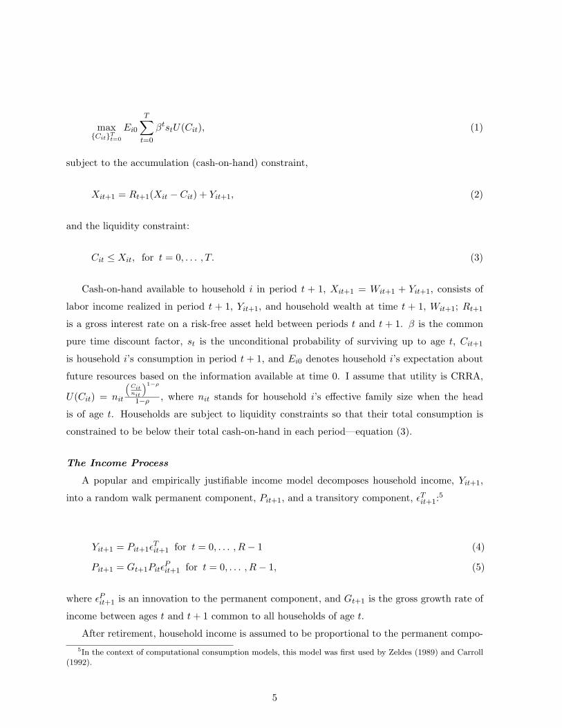
maxCitTt=0
Ei0
T∑t=0
βtstU(Cit), (1)
subject to the accumulation (cash-on-hand) constraint,
Xit+1 = Rt+1(Xit − Cit) + Yit+1, (2)
and the liquidity constraint:
Cit ≤ Xit, for t = 0, . . . , T. (3)
Cash-on-hand available to household i in period t + 1, Xit+1 = Wit+1 + Yit+1, consists of
labor income realized in period t + 1, Yit+1, and household wealth at time t + 1, Wit+1; Rt+1
is a gross interest rate on a risk-free asset held between periods t and t + 1. β is the common
pure time discount factor, st is the unconditional probability of surviving up to age t, Cit+1
is household i’s consumption in period t + 1, and Ei0 denotes household i’s expectation about
future resources based on the information available at time 0. I assume that utility is CRRA,
U(Cit) = nit
(Citnit
)1−ρ
1−ρ , where nit stands for household i’s effective family size when the head
is of age t. Households are subject to liquidity constraints so that their total consumption is
constrained to be below their total cash-on-hand in each period—equation (3).
The Income Process
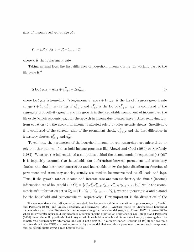
A popular and empirically justifiable income model decomposes household income, Yit+1,
into a random walk permanent component, Pit+1, and a transitory component, ϵTit+1:5
Yit+1 = Pit+1ϵTit+1 for t = 0, . . . , R− 1 (4)
Pit+1 = Gt+1PitϵPit+1 for t = 0, . . . , R− 1, (5)
where ϵPit+1 is an innovation to the permanent component, and Gt+1 is the gross growth rate of
income between ages t and t+ 1 common to all households of age t.
After retirement, household income is assumed to be proportional to the permanent compo-
5In the context of computational consumption models, this model was first used by Zeldes (1989) and Carroll(1992).
5
nent of income received at age R :
Yit = κPiR for t = R+ 1, . . . , T,
where κ is the replacement rate.
Taking natural logs, the first difference of household income during the working part of the
life cycle is:6
∆log Yit+1 = gt+1 + uPit+1 +∆uTit+1, (6)
where log Yit+1 is household i’s log-income at age t + 1; gt+1 is the log of its gross growth rate
at age t + 1; uPit+1 is the log of ϵPit+1; and uTt+1 is the log of ϵTit+1. gt+1 is composed of the
aggregate productivity growth and the growth in the predictable component of income over the
life cycle (which accounts, e.g., for the growth in income due to experience). After removing gt+1
from equation (6), the growth in income is affected solely by idiosyncratic shocks. Specifically,
it is composed of the current value of the permanent shock, uPit+1, and the first difference in
transitory shocks, uTit+1 and uTit.
To calibrate the parameters of the household income process researchers use micro data, or
rely on other studies of household income processes like Abowd and Card (1989) or MaCurdy
(1982). What are the informational assumptions behind the income model in equations (4)–(6)?
It is implicitly assumed that households can differentiate between permanent and transitory
shocks, and that both econometricians and households know the joint distribution function of
permanent and transitory shocks, usually assumed to be uncorrelated at all leads and lags.
Thus, if the growth rate of income and interest rate are non-stochastic, the time-t (income)
information set of household i is Ωhit = ϵPit , ϵTit, ϵPit−1, ϵ
Tit−1, ϵ
Pit−2, ϵ
Tit−2, . . . , Yi0 while the econo-
metrician’s information set is Ωeit = Yit, Yit−1, Yit−2, . . . , Yi0, where superscripts h and e stand
for the household and econometrician, respectively. How important is the distinction of the
6For some evidence that idiosyncratic household log income is a difference stationary process see, e.g., Meghirand Pistaferri (2004) and Guiso, Pistaferri, and Schivardi (2005). Another model of idiosyncratic householdincome advanced in the literature is the heterogenous growth-rate model (see, e.g., Baker 1997, Guvenen 2009)where idiosyncratic household log-income is a person-specific function of experience or age. Meghir and Pistaferri(2004) tested the null hypothesis that idiosyncratic household income is a difference stationary process against thegrowth-rate heterogeneity alternative and could not reject it. In a recent paper, Hryshko (2008) finds that maleearnings data in the PSID are best represented by the model that contains a permanent random walk componentand no deterministic growth-rate heterogeneity.
6
informational sets of econometricians and households? Assume a household knows that the
shocks to its permanent and transitory income are negatively correlated. For example, when the
head gets promoted, he expects his bonuses to be cut off. This (negative) correlation helps the
household sharpen its predictions on the smoothness of the unpredictable part of the income
growth, and adjust consumption appropriately. Econometricians, in turn, do not differentiate
between income news known to households, but can decompose them into orthogonal permanent
and transitory components. Consequently, econometricians make spurious conclusions about the
joint distribution of permanent and transitory components, and this may lead to their wrong
predictions of household reactions to income growth.7
Within the PIH, the correct identification of permanent versus transitory component of
income has been proven to be important. Quah (1990) showed that if econometricians observe
income news different from the news households observe, they may falsely reject the PIH, even
though households behave exactly in accordance with it. This is the main point made by
Quah (1990) that provides one of the solutions to the excess smoothness puzzle. Quah (1990)
constructs different representations of several reduced form models of the aggregate US income,
and finds that there always exists an income model consistent with the relative pattern of
variances of consumption and income observed in the aggregate US data, and consistent with
the PIH. Thus, the excess smoothness puzzle in macro data can be solved if the importance of
the permanent component is “reduced.” It is possible to suppress the permanent component
within an income model without distortion of the properties of the reduced form process.
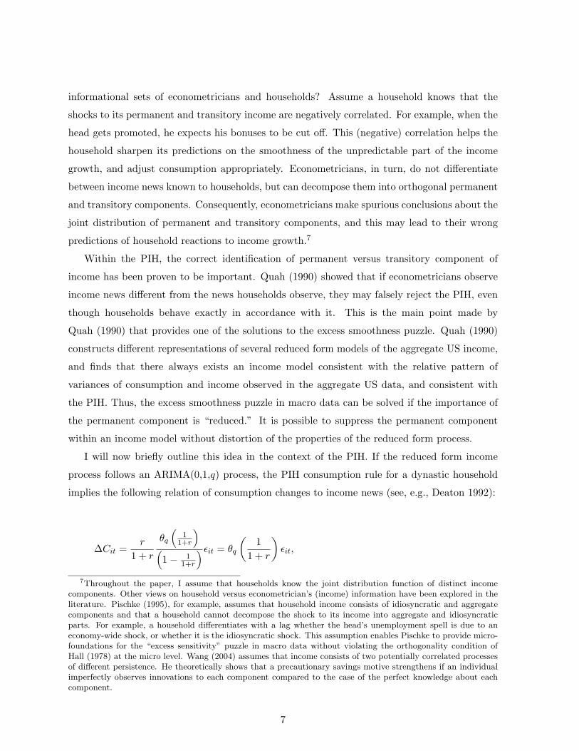
I will now briefly outline this idea in the context of the PIH. If the reduced form income
process follows an ARIMA(0,1,q) process, the PIH consumption rule for a dynastic household
implies the following relation of consumption changes to income news (see, e.g., Deaton 1992):
∆Cit =r
1 + r
θq
(1
1+r
)(1− 1
1+r
)ϵit = θq
(1
1 + r
)ϵit,
7Throughout the paper, I assume that households know the joint distribution function of distinct incomecomponents. Other views on household versus econometrician’s (income) information have been explored in theliterature. Pischke (1995), for example, assumes that household income consists of idiosyncratic and aggregatecomponents and that a household cannot decompose the shock to its income into aggregate and idiosyncraticparts. For example, a household differentiates with a lag whether the head’s unemployment spell is due to aneconomy-wide shock, or whether it is the idiosyncratic shock. This assumption enables Pischke to provide micro-foundations for the “excess sensitivity” puzzle in macro data without violating the orthogonality condition ofHall (1978) at the micro level. Wang (2004) assumes that income consists of two potentially correlated processesof different persistence. He theoretically shows that a precautionary savings motive strengthens if an individualimperfectly observes innovations to each component compared to the case of the perfect knowledge about eachcomponent.
7
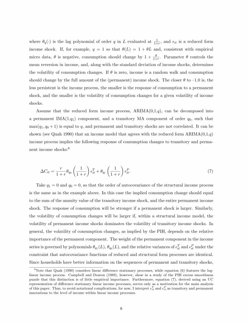
where θq(·) is the lag polynomial of order q in L evaluated at 11+r , and ϵit is a reduced form
income shock. If, for example, q = 1 so that θ(L) = 1 + θL and, consistent with empirical
micro data, θ is negative, consumption should change by 1 + θ1+r . Parameter θ controls the
mean reversion in income, and, along with the standard deviation of income shocks, determines
the volatility of consumption changes. If θ is zero, income is a random walk and consumption
should change by the full amount of the (permanent) income shock. The closer θ to –1.0 is, the
less persistent is the income process, the smaller is the response of consumption to a permanent
shock, and the smaller is the volatility of consumption changes for a given volatility of income
shocks.
Assume that the reduced form income process, ARIMA(0,1,q), can be decomposed into
a permanent IMA(1,q1) component, and a transitory MA component of order q0, such that
max(q1, q0 +1) is equal to q, and permanent and transitory shocks are not correlated. It can be
shown (see Quah 1990) that an income model that agrees with the reduced form ARIMA(0,1,q)
income process implies the following response of consumption changes to transitory and perma-
nent income shocks:8
∆Cit =r
1 + rθq0
(1
1 + r
)ϵTit + θq1
(1
1 + r
)ϵPit . (7)
Take q1 = 0 and q0 = 0, so that the order of autocovariance of the structural income process
is the same as in the example above. In this case the implied consumption change should equal
to the sum of the annuity value of the transitory income shock, and the entire permanent income
shock. The response of consumption will be stronger if a permanent shock is larger. Similarly,
the volatility of consumption changes will be larger if, within a structural income model, the
volatility of permanent income shocks dominates the volatility of transitory income shocks. In
general, the volatility of consumption changes, as implied by the PIH, depends on the relative
importance of the permanent component. The weight of the permanent component in the income
series is governed by polynomials θq1(L), θq0(L), and the relative variances of ϵTit and ϵPit under the
constraint that autocovariance functions of reduced and structural form processes are identical.
Since households have better information on the sequences of permanent and transitory shocks,
8Note that Quah (1990) considers linear difference stationary processes, while equation (6) features the log-linear income process. Campbell and Deaton (1989), however, show in a study of the PIH excess smoothnesspuzzle that this distinction is of little empirical importance. Furthermore, equation (7), derived using an UCrepresentation of difference stationary linear income processes, serves only as a motivation for the main analysisof this paper. Thus, to avoid notational complications, for now, I interpret ϵTit and ϵPit as transitory and permanentinnovations to the level of income within linear income processes.
8

one may conclude, provided the PIH is true, that the “correct” decomposition of income is the
one that matches the ratio of the variances of consumption and income growth observed in the
aggregate data with the ratio predicted by the PIH, which is not necessarily the one identified
by econometricians.
This intuition can be summarized as follows. The relative dynamics of income components is
best known to households and this unique knowledge should be reflected in household consump-
tion choices. Econometricians, in turn, make inferences on income components from identified
models of the income process which may or may not coincide with the model households “ob-
serve.” Ultimately, the importance of the income information sets should be judged by their
effect on household choices of consumption. In the next section, I provide some evidence on the
importance of this issue within a simulated buffer stock model of savings.
The autocovariance function of the reduced form process modeled as an ARIMA(0,1,q) has
q + 1 non-zero autocovariances, which is sufficient to estimate q moving average parameters,
along with the variance of the reduced form income shock. An estimable model of income may
allow at most q+1 non-zero parameters, two of which are the variances of structural shocks and
the rest determine the dynamics of each unobserved component of income, θq1(L) and θq0(L).
Thus, if the permanent component of income is a random walk and the transitory component
is a moving average process of order q − 1, one can identify the variances of transitory and
permanent shocks, and q − 1 moving average parameters; the correlation between the shocks is
not identifiable from the sole dynamics of household income.
3 Simulations of the Model
In this section, I use the PSID to estimate a reduced form ARIMA(0,1,1) income model. I then
construct several models of income that imply different permanent and transitory components
but have the same autocovariance function as the reduced form. I assume that consumers make
their consumption and savings choices in accordance with a life cycle buffer stock model, taking
into account the knowledge of the joint distribution of permanent and transitory shocks. I
further examine the effect of different income decompositions on consumption dynamics in the
buffer stock model.
Univariate Dynamics of Idiosyncratic Household Income
In this section, I present some results on the univariate dynamics of household income in
9
PSID data.9
The income measure I consider is the residuals from the cross-sectional regressions of house-
hold disposable log income on a second degree polynomial in the head’s age, and education dum-
mies.10 In the literature, it is typically labeled idiosyncratic household income. For the cross-
sectional regressions, I use information from the 1981–1997 annual family files of the PSID.11
Sample selection is described in Appendix C. Table 1 presents the autocovariance function for
the growth in household idiosyncratic income. As can be seen from the table, the autocovari-
ance function is statistically significant up to order two. This is consistent with an integrated
moving average process of order two and the findings in Abowd and Card (1989), and Meghir
and Pistaferri (2004). To simplify the computations, in the rest of the paper, I will assume that
the reduced form income process is an integrated moving average of order one. This is not at
odds with the data as the autocovariances of orders 2 and higher are small in magnitude. In
Table 2, I present estimates of the reduced form process for idiosyncratic household income.
Idiosyncratic household income is highly volatile, with a standard deviation of the reduced form
shocks of about 20% per year, and contains a strong mean-reverting component.
Constructing Different Income Models
In this section, I decompose a moving average process estimated in the previous section into
permanent and transitory components of different relative volatilities.
Assume that log income in differences, after the deterministic growth rate gt has been re-
moved, follows a stationary MA(1) process. This is consistent with an income process represented
as the sum of a random walk permanent component and a transitory white noise process. This
particular income process has become the workhorse in simulations of the buffer stock model of
savings and for computational models of asset holdings over the life cycle.12 The reduced and
structural forms of the process for the first differences in income are:
9I will describe the data utilized in more detail in the next section and Appendix C.10My specification of the predictable component of labor income is quite flexible: it assumes, for example,
time-varying returns to experience and education.11The PSID collected data biennially after 1997. Inclusion of data after 1997 would require a different modeling
strategy, e.g., analyzing idiosyncratic income growth over the two-year horizon. Since this strategy will necessarilyresult in a loss of data, I use the data available at the annual frequency.
12Ludvigson and Michaelides (2001) use this process to analyze “excess smoothness” and “excess sensitivity”puzzles on the aggregated data from a simulated buffer stock model; Michaelides (2001)—to investigate thesame phenomena but for a buffer stock economy of consumers with habit forming preferences; Luengo-Prado(2007)—to analyze a buffer stock model augmented with durable goods. Luengo-Prado and Sørensen (2008) usea generalization of this process to explore the effects of different types of risk (idiosyncratic and aggregate) onthe marginal propensity to consume in the simulated “state”-level data and US state-level data. Gomes andMichaelides (2005) and Cocco, Gomes, and Maenhout (2005) calibrate the parameters of this income process toinvestigate consumption and portfolio choice over the life cycle.
10
∆log Y rfit = (1 + θL)uit
∆log Y sfit = uPit + (1− L)uTit,
where superscripts rf and sf denote the reduced and structural form, respectively.
Since the reduced form has only two pieces of information, the autocovariances of order zero
and one, one can statistically identify only two parameters, the variance of permanent shocks
and the variance of transitory shocks. To explore the impact of the structure of income on the
consumption process, I allow for a covariance between the permanent and transitory shocks, and
then work out the variance of transitory shocks. I match the moments of constructed series to
the moments of the reduced form series, thus keeping the stochastic structure of the series intact.
I present the full details of the procedure in Appendix A. I take the estimated parameters of an
ARIMA(0,1,1) process from Table 2. The grid of covariances considered in simulations implies
the following correlations between structural shocks: –1.0, –0.75, –0.5, –0.25, 0.0, 0.25, 0.5, 0.75,
and 1.0. For the estimated income parameters, an estimate of the variance of innovations to the
random walk permanent component equals (1+ θ)2σ2u = 0.02. The variance of transitory innova-
tions can be estimated by −γ(1)−cov(uPit , uTit), where γ(1) is the first order autocovariance of the
reduced form process and cov(uPit , uTit) is the covariance between permanent and transitory inno-
vations. Thus, for the covariance equal to −0.0109 (and the corresponding correlation between
income shocks approximately equal to −0.50), the standard deviation of transitory innovations
is 0.152; for the covariance equal to 0.00, the standard deviation of transitory innovations is
0.111.
The decompositions differ in terms of the relative volatility of permanent and transitory
shocks. Thus, the income model with perfect negative correlation between permanent and
transitory shocks has the most volatile transitory shocks, while the income model with perfect
positive correlation has the least volatile transitory shocks.
Results for Simulated Life Cycle Buffer Stock Economies
I solve the model introduced in the previous section by utilizing the Euler equation linking
marginal utility from consumption in adjacent periods. I assume that the gross interest rate
Rt is non-stochastic and the joint probability density function of transitory and permanent
shocks is time-invariant. In addition, shocks are assumed to be jointly log-normal. I further
assume that households start their life cycle at age 26 (t = 0 in the model), retire at age 65,
11

and die with certainty at age 90 (T = 64 in the model). Before retirement, the unconditional
probability of survival is set to 1; after the retirement, households face an age-dependent risk
of dying. The conditional probabilities of surviving up to age t provided the household is alive
at age t − 1 for all R < t ≤ T − 1 are taken from Table A.1 in Hubbard, Skinner, and Zeldes
(1994).13 The replacement rate κ is set to 0.60. This value is similar to an estimate of the
replacement rate for U.S. high school graduates in Cocco, Gomes, and Maenhout (2005). The
average effective family size over the life cycle, nt, is estimated using PSID data following Scholz,
Seshadri, and Khitatrakun (2006) as (no. adultst + 0.7× no. childrent)0.7, where “no. adultst”
(“no. childrent”) is the “typical” number of adults (number of children) when household head
is of age t. The age-dependent deterministic growth rate in household disposable income, Gt,
is estimated using CEX data. I discuss construction of those profiles in the empirical section of
the paper.
After I find the age-dependent consumption functions, I simulate the economy populated
by 5,000 ex ante identical consumers, who are differentiated ex post due to different history of
income draws. I assume that households have zero wealth in the beginning of their life cycle,
at age 26. Since I am interested in the properties of consumption for different decompositions
of a given reduced form model of income, I hold all other parameters of the buffer stock model
fixed. Thus, in my first set of simulations, I do not vary the behavioral parameters of the model.
I set the gross real interest rate to 1.03, the time discount factor to 0.85, and the coefficient
of relative risk aversion to 6.0. I choose low patience and high degree of risk aversion since I
will later estimate similar values using PSID data. Those values are also consistent with the
estimates in Cagetti (2003) who used wealth data to fit a life cycle model. I take draws from the
joint distribution of log-normal transitory and permanent shocks, the parameters of which are
derived from the reduced form ARIMA(0,1,1), as already discussed in the previous subsection.
The details of the model solution are provided in Appendix B.
I run pooled panel regressions of the growth of household consumption on the growth of
household income over one and four-year horizons. The magnitude of the coefficient on the
current income growth should depend on the smoothness of income innovations. Long differences
in log income will be largely dominated by the permanent shocks, which should be reflected in
the long differences in log consumption. In the empirical evaluation of the model, I will match
the wealth-to-income ratio over the life cycle. This information is important to identify the
time discount factor and the coefficient of relative risk aversion as shown in Cagetti (2003).
Matching the wealth-to-income ratio also provides some discipline on the ability of households
13This is the mortality data on women for 1982.
12
to smooth consumption using their own assets before other forms of insurance are allowed for.
Thus, in addition to the moments that describe the sensitivity of consumption to income shocks,
I tabulate the average wealth-to-income ratio at ages 31–35 and 61–65, and the reduced form
income parameters, an autoregressive persistence and the variance of income growth. The results
for income models with negative correlation, no correlation, and positive correlation between
the shocks are presented in Table 4.14
In the first three rows of Table 4, I show that consumption is contemporaneously less sensitive
to income when the correlation between the shocks is the lowest. Similar results hold for the
sensitivity of consumption growth to income growth over the four-year horizon. The average
wealth-to-income ratio at early and late stages of the working part of the life cycle is not affected
much by the choice of the income process.
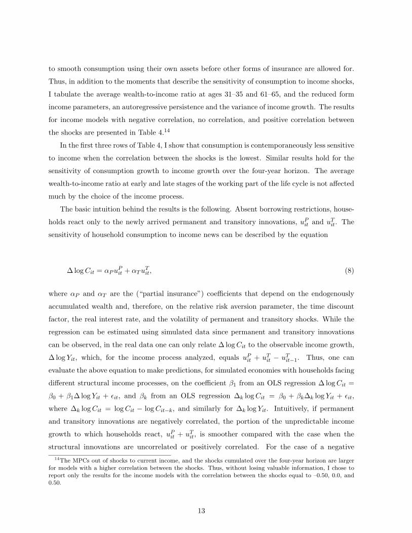
The basic intuition behind the results is the following. Absent borrowing restrictions, house-
holds react only to the newly arrived permanent and transitory innovations, uPit and uTit. The
sensitivity of household consumption to income news can be described by the equation
∆ logCit = αPuPit + αTu
Tit, (8)
where αP and αT are the (“partial insurance”) coefficients that depend on the endogenously
accumulated wealth and, therefore, on the relative risk aversion parameter, the time discount
factor, the real interest rate, and the volatility of permanent and transitory shocks. While the
regression can be estimated using simulated data since permanent and transitory innovations
can be observed, in the real data one can only relate ∆ logCit to the observable income growth,
∆ log Yit, which, for the income process analyzed, equals uPit + uTit − uTit−1. Thus, one can
evaluate the above equation to make predictions, for simulated economies with households facing
different structural income processes, on the coefficient β1 from an OLS regression ∆ logCit =
β0 + β1∆log Yit + ϵit, and βk from an OLS regression ∆k logCit = β0 + βk∆k log Yit + ϵit,
where ∆k logCit = logCit − logCit−k, and similarly for ∆k log Yit. Intuitively, if permanent
and transitory innovations are negatively correlated, the portion of the unpredictable income
growth to which households react, uPit + uTit, is smoother compared with the case when the
structural innovations are uncorrelated or positively correlated. For the case of a negative
14The MPCs out of shocks to current income, and the shocks cumulated over the four-year horizon are largerfor models with a higher correlation between the shocks. Thus, without losing valuable information, I chose toreport only the results for the income models with the correlation between the shocks equal to –0.50, 0.0, and0.50.
13
correlation, a positive permanent shock is, on average, accompanied by a negative transitory
shock, smoothing out the sum of income innovations. Hence, income becomes smoother and
this is reflected in lower coefficients measuring the sensitivity of current consumption to current
income growth (β1), and cumulative consumption growth to cumulative income growth over the
four-year horizon (β4). For the case of a positive correlation, positive (negative) permanent
shocks arrive, on average, together with positive (negative) transitory shocks, making the sum
of innovations less smooth and this is consequently reflected in higher coefficients measuring the
sensitivity of consumption to income growth at different horizons (β1 and β4). In statistical
terms,
β1 =cov(∆ logCit, ∆ log Yit)
var(∆ log Yit)=
αPσ2uP + αTσ
2uT + (αP + αT )cov(u
Pit , u
Tit)
var(∆ log Yit).
The denominator is the same for all structural decompositions of the reduced form income
model, the “smoothing” term is measured by (αP +αT )cov(uPit , u
Tit) in the numerator. It follows
that the sensitivity of current consumption to current income growth is lower for structural in-
come models with more negatively correlated shocks. The sensitivity of cumulative consumption
growth to cumulative income growth over k periods is measured by
βk =kαPσ
2uP + αTσ
2uT + (αP + kαT )cov(u
Pit , u
Tit)
kσ2uP + 2σ2
uT + 2cov(uPit , uTit)
.
Again, the denominator is the same for different structural income processes while the nu-
merator contains the “smoothing” term (αP + kαT )cov(uPit , u
Tit), which is larger, in absolute
value, for the processes with more negatively correlated permanent and transitory shocks.
In rows (4) and (5), I explore the sensitivity of the moments in the benchmark model in
row (1) to different values of the risk aversion parameter. Lower risk aversion results in a much
lower accumulation of assets over the life cycle—households arrive with virtually no assets at
retirement when the coefficient of relative risk aversion is set to 2 and the degree of impatience
is kept at a high level. As a result, households are very sensitive to income shocks, as reflected
in high values of β1 and β4. The reverse is true for a higher degree of risk aversion. In rows (5)
and (6), I examine the sensitivity of the model moments to variations in the time discount factor,
holding other parameters at their values in row (1). The results are intuitive: more patient
consumers accumulate larger amounts of wealth and are able to better smooth consumption
14
over the life cycle.
Lastly, in rows (8)–(10) I explore the effect of introducing partial risk sharing against per-
manent and/or transitory income shocks on the model moments. I do not model risk sharing in
a structural way. Rather, I follow Attanasio and Pavoni (2011) who show, for a model with hid-
den access to asset markets, that the bond (self-insurance) Euler equation holds for household
resources that have been smoothed by state-contingent transfers or other mechanisms before
households make their decisions on savings. The sensitivity of consumption to income shocks
at one and four-year horizons is halved when 50 percent risk sharing of permanent and tran-
sitory shocks are allowed in the model. The results are similar when partial risk sharing of
permanent income shocks only is introduced into the model—row (9). Households appear to
substantially smooth transitory shocks using accumulated assets (for a similar result, see Kaplan
and Violante 2010). Consumption reaction to income shocks is similar to the no-insurance case
when households do not have access to partial risk sharing of permanent income shocks but 50
percent of transitory shocks are smoothed away before self-insurance—rows (1) and (10). Thus,
the model moments are not affected much by the availability of partial risk sharing of transi-
tory shocks. It can be concluded that partial risk sharing of transitory income shocks beyond
self-insurance is not likely to be well identified empirically. In the empirical section, therefore, I
will estimate the degree of risk sharing of permanent shocks only.
Summarizing, there is substantial variation of the model moments with respect to changes in
the income process parameters, behavioral and risk-sharing parameters. It appears possible to
identify the model parameters by matching the data moments to the same moments estimated
within the model.
4 Estimation of the Model
In this section, I use a life cycle model of consumption to estimate the parameters of the income
process and the behavioral parameters. I assume that model households are married couples who
maximize expected utility from consumption over the life cycle. The only source of uncertainty
in the model before retirement is uncertainty over the flows of income, arising from transitory
and permanent income shocks. I assume that all households start working at age 26 and retire
at age 66.
As in previous section, I assume that households have access to one instrument for saving
and consumption smoothing—a riskless bond with the deterministic gross interest rate R. Cash-
on-hand accumulation constraint and the income process are given in equations (2), and (4)–(6)
15
respectively. I assume that households are subject to liquidity constraints so that their total
consumption is constrained to be below their total cash-on-hand in each period.
Cash-on-hand and consumption at age t can be expressed in terms of the ratios to the
permanent component of income at age t, and the state space of the corresponding dynamic
programming problem reduces to one variable, cash-on-hand relative to the permanent income,
xit. The details of the model solution are provided in Appendix B.
Matching Empirical Moments
In this section, I describe the method used to estimate the structural parameters of the
model. The vector of structural parameters θ consists of the behavioral parameters—β, ρ;
the parameters of the income process—σuT , σuP and corr(uPituTit); and the partial risk sharing
parameters, ωP and ωT . I estimate the model parameters by the method of simulated moments.
I recover the parameters by matching the empirical moments listed in Table 5. I match
fifteen moments in total (enumerated in the table). Since the model does not provide a closed-
form solution for these moments, I simulate the moments and estimate the parameters of the
model by matching these simulated moments to the data moments. I estimate the model in
two stages. In the first stage I estimate the exogenous parameters χ, I then fix them in the
MSM optimization routine; in the second stage I estimate, within the MSM routine, the model
parameters θ. χ consists of the life cycle profile of the (deterministic) gross growth rates of
disposable income, Gt65t=26; the life cycle profile of the effective family size, nt66t=26; the mean
and standard deviation of the distribution of the permanent component of household disposable
income at age 26;15 and the variance of measurement error in household total expenditures. I
set the gross real interest rate on safe liquid assets to 1.03.
Given the estimates of the first stage parameters, the MSM estimates of the second stage
parameters θ are such that the weighted distance between the vector of simulated moments
and the vector of empirical moments is as close to zero as “possible.” θ is the solution to the
minimization of the following criterion function
[logms(θ; χ)− logmd
]′W
[logms(θ; χ)− logmd
]= g′IsWgIs ,
where superscript d denotes data; s denotes simulation; Id is the number of households in the
data contributing towards estimation of the second-stage moments; Is is the number of simulated
households; md is a vector of the second-stage moments estimated from the data; ms(θ; χ) is
15I set those to the mean and variance of the distribution of household disposable income at age 26.
16
a vector of simulated moments; W is a positive definite weighting matrix; χ is a vector of the
preestimated first-stage moments; θ is a vector of the second-stage parameters.
Construction of Empirical Moments and Life Cycle Profiles
In this section, I describe estimation of the empirical moments I match. I first briefly describe
the data sources used. I obtain consumption information from two data sources, the CEX and
the PSID. The CEX contains detailed information on total expenditures and its components, and
the demographics for representative cross sections of the US population. I use extracts from the
1980–2003 waves of the CEX available at the National Bureau of Economic Research (NBER)
webpage. Unlike the CEX, the PSID provides panel data yet limits its coverage of consumer
expenditures to food at home and away from home. Since I am interested in the link between
changes of household disposable income and total household consumption, I impute the total
consumption to the sample PSID households using information on household food consumption
in the PSID and the CEX, and matched demographics from the CEX and the PSID. PSID data
are taken from 1981–1997, 1999, 2001, and 2003 waves. I follow the methodology of Blundell,
Pistaferri, and Preston (2005) to impute total consumption to the PSID households. The full
details on sample selection of CEX and PSID households are provided in Appendix C. Briefly,
from the PSID, I choose married couples headed by males of ages 26–70 born between 1912 and
1978, with no changes in family composition (no changes at all or changes in family members
other than the head and wife). I drop income outliers, observations with missing or zero records
on food at home and, for each household, keep the longest period with consecutive information on
household disposable income and no missing demographics. From the CEX, I choose households
who are complete income and expenditure reporters, with heads who belong to the same age
groups and cohorts as in the PSID sample.
In the PSID, federal income taxes are calculated by staff until 1991. To have a consistent
measure of federal income taxes for the data that extend beyond 1991, one needs to impute them
to the PSID households. I use the TAXSIM tool at the NBER to calculate federal income taxes
and social security withholdings for the head and wife and all other family members if present. I
use information on imputed household disposable income for estimation of the moments listed in
Table 5. I use CEX data to construct the profile of the life-cycle growth in household disposable
income. In the CEX, federal income taxes and taxable household income are reported rather
than imputed. Thus, the profile of the deterministic life-cycle growth in household disposable
income can be more reliably estimated using CEX data.
I decompose household disposable log income into cohort, time, and age effects, controlling
17

for the effect of family size. As is well known, age, cohort, and time effects are not separately
identified. I follow Deaton (1997) and restrict the time dummies to be orthogonal to a time
trend and to add up to zero. The age effects from such regression, smoothed using a fifth-degree
polynomial, are depicted in panel (a) of Figure 1.16 Household disposable income peaks at age
52. The profile of deterministic growth in household disposable income, Gt, is obtained by taking
the difference between the adjacent points in the figure.
Attanasio, Banks, Meghir, and Weber (1999) showed the importance of controlling for chang-
ing family size over the life cycle in a model with income uncertainty and self-insurance. I calcu-
late the effective family size for household i at age t as nit = (no. adultsit + 0.7× no. childrenit)0.7,
following Scholz, Seshadri, and Khitatrakun (2006). I use PSID data to construct the life cycle
profile of the effective family size.17 I run a regression that controls for household fixed effects,
age effects, and time effects.18 As with household income data, I assume that the time dummies
are orthogonal to a time trend and sum to zero. The age effects, smoothed using a fifth-degree
polynomial, are depicted in panel (b) of Figure (1). The effective family size peaks at age 40.
In Table 3, I present the autocovariance function of idiosyncratic growth rate of household
total (imputed) consumption.19 I utilize data from the 1981–1997 surveys of the PSID. I run
cross-sectional regressions of the first difference in household log consumption on a quadratic
polynomial in the head’s age and the change in family size. The residuals from those regres-
sions are labeled idiosyncratic consumption growth. Only the first-order autocovariance of con-
sumption growth is significant; higher-order autocovariances are small in magnitude and not
significant. The variance of idiosyncratic consumption growth is large in magnitude, which can
be partly explained by the variance of measurement and imputation error in consumption. In
theory, household consumption is a martingale unless consumption is measured with error, in
which case the first-order autocovariance of consumption growth will be negative. I assume that
the variance of measurement and imputation error in consumption is equal to 0.08, the negative
of the estimated value of the first-order autocovariance in idiosyncratic consumption growth.
In panel (c) of Figure 1, I plot the life cycle profile of the wealth-to-income ratio. I use
household net worth exclusive of business wealth, and household disposable income to construct
this measure. Relative to the household income and family size data, I do not have as much
data for construction of the wealth profile. For the time span of my sample, the wealth data
16The omitted age group in the regression are the heads of age 26. Thus, the depicted age effects should beinterpreted as the average log income at ages 27, . . . , 65 relative to the average log income at age 26.
17The profile is similar if CEX data are used instead.18If household fixed effects are included, the cohort effects are not identified.19It is similar to the autocovariance function of consumption growth in Blundell, Pistaferri, and Preston (2008).
18
are recorded only in six supplements, collected every five years from 1984 to 1999, and every
other year afterwards. The time effects, restricted as above, are unlikely to be identified.20
Because of a small number of wealth observations at different ages, especially at older ages, I
run a regression of the wealth-to-income ratio on a limited set of age dummies, controlling for
household fixed effects. I consider 8 age dummies. Each age dummy comprises households who
fall into one of the 8 five-year age intervals: 26− 30, . . . , 61− 65. The results of this regression
are provided in Table 5 and depicted in panel (c) of Figure 1. Households start with low wealth
in the beginning of the life cycle and have wealth exceeding their income by more than 4.5 times
when they approach retirement. In the model, I assume that households start with zero wealth
at age 26. To eliminate the influence of this assumption on the results, I do not match the
wealth moment calculated for ages 26–30.
The other moments used for matching measure the extent of smoothness of consumption with
respect to income changes, and the variance of idiosyncratic income growth and the persistence
of household disposable income. The consumption smoothness is measured by the coefficients
βj , j = 1, . . . , 4, from the following panel regressions estimated by OLS:
∆j log cit = β0 + βj∆j log yit + γ′xit + ϵit,
where zit ≡ Zit−Zt for any variable z in the regression, ∆j log zit ≡ log zit− log zit−j , and xit is
a vector that comprises a quadratic polynomial in the head’s age, and family size. I take out the
time-specific averages from the variables since I do not have aggregate uncertainty in the model.
The estimated value of β1 suggests that about 12 percent of the shocks to current income are
translated into consumption—row (8) of Table 5. This can be due to the presence of a large
transitory component in income, measurement error in income, or different insurance mecha-
nisms available to households for smoothing out fluctuations in disposable income. Households
react to about 23 percent of income shocks cumulated over the four-year horizon, as indicated
by the estimated value of β4—row (11) of Table 5.
If permanent and transitory shocks are uncorrelated and the transitory component is an iid
process, the following respective moments will identify αP and αT in equation (8) (see, e.g.,
Kaufmann and Pistaferri 2009):E(ϵcitϵ
yit)+E(ϵcitϵ
yit+1)
E(ϵyit)2+2E(ϵyitϵ
yit+1)
andE(ϵcitϵ
yit+1)
E(ϵyitϵyit+1)
, where ϵcit (ϵyit) is the first
difference in residuals from a regression of log consumption (income) on dummy variables for
20The life cycle profile of the wealth-to-income ratio is similar if I simply take out the time-specific means fromthe ratio and then run a regression controlling for age and household fixed effects.
19
the head’s year-of-birth, high school and college, race, family size, Census region, number of kids,
employment status, as well as interactions of those dummies (but race) with year dummies. For
matching, I use (1−αP ) and (1−αT ) as the data estimates of partial insurance against permanent
and transitory shocks; I denote them as ϕP and ϕT , respectively. I find that households smooth
out about 40% (100%) of permanent (transitory) shocks to their disposable incomes—rows (12)–
(13) of Table 5. Similar estimates, but for a different sample, have been found in Blundell,
Pistaferri, and Preston (2008). Ideally, a successful model should match both the reaction of
consumption to income shocks at different horizons (β-coefficients) and the partial insurance
moments (ϕP and ϕT ).
I match the AR(1) coefficient of the reduced form process rather than an MA(1) estimate,
since an AR(1) process is less time consuming to estimate. This proves to be very important
when repeated estimations are performed on simulated data. Specifically, I match the value of
α estimated from the following regression:
∆ log yit = α0 + α∆log yit−1 + γ′xit + ϵit,
where xit is a vector that includes a quadratic polynomial in the head’s age and dummies for
the head’s high school graduation and college completion. As in the previous regressions, I take
out the time-specific means from each variable prior to running the regression.
The size of income risk over the life cycle is calculated as the variance of idiosyncratic income
growth. For its estimation, I first run cross-sectional regressions of the difference in household
log disposable income on a quadratic polynomial in the head’s age and dummies for high school
and college using data from the 1981–1997 surveys, when household income was continuously
recorded each year. I limit the regression sample to the households with heads of ages 26–65.
The unconditional variance of the residuals from those regressions provides an estimate of the
proportional risk to household disposable income over the life cycle. The estimated variance
along with its standard error are shown in row (14) of Table 5.
Further details on the model solution, and calculation of standard errors are provided in
Appendix B.
20
5 Results
Table 6 contains the main results. The values of the data moments reported in Table 5 are
replicated for convenience in square brackets in the bottom of Table 6.
I first assume that transitory and permanent shocks are uncorrelated and target the wealth
moments, income moments, and the reaction of consumption to current income shocks—column (1).
The coefficient of relative risk aversion is estimated at about 7, and the time discount factor at
about 0.81: households exhibit low patience and high degree of risk aversion. The estimated
value of the time discount factor compares well with Cagetti (2003); the relative risk aversion
parameter is comparable in magnitude with the estimates in Cagetti (2003) and Nielsen and
Vissing-Jorgensen (2006). The size of permanent shocks to household disposable income and
the size of transitory shocks are tightly estimated: one standard deviation in permanent shocks
equals about 14 percent, while one standard deviation in transitory white-noise shocks equals 12
percent.21 The wealth moments, the variance of income risk and the persistence of risk are well
fitted to the corresponding data moments.22 Consumption, however, appears to be excessively
smooth: consumption is more than twice as sensitive to current income shocks and shocks cumu-
lated over the four-year horizon as in the data; in the data, households appear to smooth away
twice as much permanent shocks as in the model. As emphasized in the simulation section, the
consumption smoothness moments can be better explained if households have access to some
insurance mechanisms other than self-insurance via accumulation of wealth, or if they react
to smoother income components, the dynamics of which agree with the reduced form income
moments but cannot be detected by using the income data alone. I first examine if the second
mechanism is enough to explain the consumption smoothness moments found in the data.
In column (2), I allow components of income to be contemporaneously correlated. I precisely
estimate the negative correlation between permanent and transitory shocks of about –0.61. The
fit of the model improves, as reflected in a lower value of the goodness-of-fit statistics, and the
model is able to explain the reaction of consumption to the shocks to current income, along with
the wealth moments and income moments. The model, however, fails at predicting the reaction
of household consumption to the income shocks cumulated over the four-year horizon as well as
the moment relating to partial insurance against permanent shocks, ϕP . That is, consumption
21These values are similar to the estimates of the income process using data on household idiosyncratic incomegrowth alone.
22In columns (1) and (3) of Tables 6–7, to better match the income moments I placed relatively larger weights tothe income moments in the weighting matrix while using equal weights for the wealth and consumption smoothnessmoments. The reason for this choice is that I wanted model households to face exactly the same amount of risk andits persistence as seen in the data, and to explore the performance of the model with respect to the consumptionsmoothness moments, while fitting the income and wealth moments as close as possible.
21
is still excessively smooth.
There are some plausible explanations for the correlation between structural income shocks
found in the data. The sign of the covariance may indicate that unfavorable permanent shocks to
disposable household income, such as the head’s long-term unemployment, are partially offset by
increases in the transitory income such as unemployment compensation from the government. It
is also likely that this offsetting effect will manifest itself at the annual frequency, the frequency
I use for modeling consumption in the life cycle model. Consider another explanation for this
finding. Household income derives from multiple sources: the wage of wife and head, transfer
income of various sorts, (labor part of) business and farm income, (labor part of) income from
roomers and boarders, bonuses, overtime and tips. As an example, if a household experiences a
negative shock to the head’s wages, plausibly assumed to be in the list of permanent shocks, it
may compensate the adverse effect by temporarily leasing available housing. In a recent paper,
Belzil and Bognanno (2008) find that increases in the base pay (positive permanent shocks) for
American executives are followed by bonus cuts (negative transitory shocks). They argue that
this phenomenon (of the negative correlation between the shocks) may reflect a compensation-
smoothing strategy on the part of firms’ managers.23
In column (3) of Table 6 I match all moments in Table 5, allowing for both household infor-
mation about the (potentially correlated) income components and partial risk sharing against
permanent income shocks. Previous results are based on fitting empirical data moments to
the same moments from a life cycle model that features self-insurance. In the model, house-
holds have access only to one vehicle of consumption smoothing over the life cycle, the risk-free
bond. In reality, households may rely on other insurance mechanisms, e.g., state contingent
assets and transfers of different sorts, that is, their permanent and transitory idiosyncratic
shocks may be partially insured. In a recent paper, Attanasio and Pavoni (2011) showed, for
a partial risk sharing model with moral hazard and hidden asset accumulation, that the self-
insurance Euler equation still holds if applied to the “after-risk-sharing” income.24 To account
23Jacobson, LaLonde, and Sullivan (1993), for a sample of high-tenure workers, find that job displacement resultsinto an initial drop of about 50% of pre-displacement earnings; eventually earnings recover but they are still 25%below their pre-displacement levels in 6 years. If one is willing to make an inference that the permanent shockequals 25%, then, at the arrival of the displacement event, this negative permanent shock should be accompaniedby a negative transitory shock. Thus, contrary to this paper’s finding the correlation between the shocks shouldbe positive. However, the displacement event is just one among the very many events that cause permanentvariations in incomes. Moreover, it is quite infrequent, with the annual likelihood of occurrence of about 4%. SeeKrebs (2003) for a review of the literature on the effect of displacements on earnings. In this paper I find that,on average, permanent and transitory shocks comove in different directions, and this negative comovement helpsreconcile the reaction of consumption to income observed in the data. The negative correlation is not inconsistentwith an observation that some permanent and transitory shocks move in the same direction.
24There can be other market structures that allow for partial risk sharing. I consider the one proposed by At-tanasio and Pavoni (2011) since it is easy to integrate it into the model in the “reduced-form” way.
22

for partial risk sharing, I model the after-risk-sharing household income as Yit = PitϵTit, where
Pit = GtPit−1
(ϵPit
)ωP , and 1 − ωP is the fraction of permanent shocks that is smoothed out
before households make their decisions on asset holdings. I do not consider partial risk sharing
of transitory shocks since those are well insured by means of self-insurance.25 The life-cycle path
of the average wealth-to-income ratio in the data and model are plotted in Figure 2, panel (a).
The profiles align quite well. In panel (b), I plot the profile of consumption over the life cycle
implied by the model estimates in column (3) of Table 6. Consumption has a visible hump and
peaks at around age 50. The hump and the timing of the peak in different measures of house-
hold consumption is documented in many studies—see, e.g., Fernandez-Villaverde and Krueger
(2007). The estimates of the time discount factor and the coefficient of relative risk aversion do
not change appreciably.
Relative to column (2), I estimate a somewhat lower standard deviation of transitory shocks
and correlation between the shocks, both significant at the 2% level. The model in column (3) fits
well the profile of consumption adjustment to the shocks over different horizons (β-coefficients)
but overestimates the moments relating to partial insurance of permanent and transitory shocks;
I estimate that about 52 percent of permanent shocks are insured before self-insurance.
In Table 7, I repeat the same analysis assuming that measurement error in income explains 25
percent of idiosyncratic income growth.26 This results in lower estimates of the size of transitory
shocks, and less precisely estimated correlation between the shocks when partial risk sharing of
permanent shocks is allowed for—the correlation is still significant at the 8% level. The size of
permanent shocks is estimated at about the same value.27 The estimates of the time discount
factor, the coefficient of relative risk aversion, the correlation between the shocks and partial
insurance of permanent shocks are very similar in magnitude.
It may be the case that a more superior fit of the wealth and β-moments is due to the equal
weighting scheme and a relatively larger amount of those moments. In column (4) of Table 7,
therefore, I fit two wealth moments (average wealth for ages 31–45 and ages 46–65), two β-
moments (consumption reaction to income shocks cumulated over one and four-year horizons),
two income process moments, and two partial insurance moments. As a result, the fit of the
model to the moment relating to partial insurance of permanent shocks improves but the model
25As shown in Table 4, partial risk sharing of transitory shocks is not likely to be empirically identified sincethe moments barely change when I allow for it in the model.
26This is consistent with the literature on measurement error in individual earnings surveyed in Bound, Brown,and Mathiowetz (2001). I am not aware of research on the extent of measurement error in household disposableincome.
27This result is consistent with the theory: if log income contains a random-walk component, the volatility ofpermanent shocks should be identified for any covariance-stationary model of the transitory component, and anyvalue of the contemporaneous correlation between permanent and transitory shocks—see, e.g., Cochrane (1988).
23
still overestimates this moment.
It is possible to provide direct evidence on the correlation between the shocks if both data
on household expectations and realizations of income growth are available for several years.
This information is not available in the U.S. but can be found in Italian data from the Survey of
Household Income and Wealth (SHIW). Pistaferri (2001), using these data, identifies permanent
and transitory shocks and tests the PIH by studying the reaction of household savings to the
shocks. I use income and demographic data for individuals from the 1995, 1998, and 2000 waves
of the SHIW. The first two waves contain individual records on one-year ahead expectations of
non-financial income. I utilize the sample comprising individuals with non-missing information
on income expectations in the 1995 and 1998 waves, and non-missing information on income
realizations in all three waves. I find the correlation between transitory and permanent shocks of
about –0.45 (–0.39) with a bootstrapped standard error of 0.11 (0.18) for the whole (heads-only)
sample.28 It appears that my findings using a matching exercise are in accord with the findings
using survey data, with a qualification that they are based on data from different developed
countries.
6 Conclusion
In an estimated life cycle model with self-insurance, I find that household consumption is ex-
cessively smooth. To reconcile the model with the data, I suggest that households have better
information about income components than econometricians. In this case, the structure of the
income process that econometricians can identify from the univariate dynamics of household
income may differ from the true income structure.
When permanent and transitory shocks are contemporaneously negatively correlated, the
unpredictable part of income growth, to which households react, is smoother compared with
the case of zero and positive correlation between the shocks. Likewise, consumption becomes
smoother and this is reflected in lower sensitivities of consumption to current income shocks, and
shocks cumulated over longer horizons. This mechanism allows me to identify the correlation
in the data and to better fit the consumption smoothness moments. Consumption, however, is
still excessively smooth in the data compared to the model. The model is able to replicate the
28For these data, I can directly identify the correlation between the sum of permanent shocks in years 1996–1998and the transitory shock in 1998—details are available upon request. Assuming that the variance of permanentand transitory shocks, as well as the covariance between the shocks are time-invariant, I can further identify thecorrelation between the shocks, which is reported in the text. If the transitory component is an MA(1) process,an estimate of the reported correlation is biased towards zero.
24

reaction of consumption to current income growth, while the reaction of consumption to income
growth over the four-year horizon is larger in the model than in the data.
The model is consistent with income, wealth, and consumption smoothness moments esti-
mated from CEX and PSID data when I allow for household information about components
of income and partial risk sharing against permanent income shocks. The precautionary sav-
ings motive found to be important for understanding household wealth accumulation in Cagetti
(2003) and Gourinchas and Parker (2002) is not enough to explain the smoothness of consump-
tion that households are able to achieve in the data. More research is needed to understand
insurance mechanisms available to U.S. households, besides those provided publicly in the form
of miscellaneous public transfers and progressive taxation.
25
References
Abowd, J., and D. Card (1989): “On the Covariance Structure of Earnings and HoursChanges,” Econometrica, 57, 411–445.
Attanasio, O., J. Banks, C. Meghir, and G. Weber (1999): “Humps and Bumps inLifetime Consumption,” Journal of Business and Economics Statistics, 17, 22–35.
Attanasio, O., and N. Pavoni (2011): “Risk Sharing in Private Information Models withAsset Accumulation: Explaining the Excess Smoothness of Consumption,” Econometrica, 79,1027–1068.
Baker, M. (1997): “Growth-Rate Heterogeneity and the Covariance Structure of Life-CycleEarnings,” Journal of Labor Economics, 15, 338–375.
Belzil, C., and M. Bognanno (2008): “Promotions, Demotions, Halo Effects, and the Earn-ings Dynamics of American Executives,” Journal of Labor Economics, 26, 287–310.
Blundell, R., L. Pistaferri, and I. Preston (2005): “Imputing Consumption in the PSIDUsing Food Demand Estimates from the CEX,” IFS Working Paper #04/27.
(2008): “Consumption Inequality and Partial Insurance,” American Economic Review,98(5), 1887–1921.
Bound, J., C. Brown, and N. Mathiowetz (2001): “Measurement Error in Survey Data,”in Handbook of Econometrics, Vol.5, chap. 59, pp. 3705–3843. North-Holland, New York.
Cagetti, M. (2003): “Wealth Accumulation Over the Life Cycle and Precautionary Savings,”Journal of Business and Economics Statistics, 21, 339–353.
Campbell, J. Y., and A. Deaton (1989): “Why is Consumption so Smooth?,” Review ofEconomic Studies, 56, 357–374.
Carroll, C. D. (1992): “The Buffer-Stock Theory of Saving: Some Macroeconomic Evidence,”Brookings Papers on Economic Activity, 2, 61–156.
(2001): “Precautionary Saving and the Marginal Propensity to Consume Out of Per-manent Income,” NBER Working Paper # 8223.
(2006): “The Method of Endogenous Gridpoints for Solving Dynamic Stochastic Op-timization Problems,” Economics Letters, 91, 312–320.
Carroll, C. D., and A. A. Samwick (1997): “The Nature of Precautionary Wealth,” Journalof Monetary Economics, 40, 41–71.
Cocco, J., F. Gomes, and P. Maenhout (2005): “Consumption and Portfolio Choice Overthe Life Cycle,” Review of Financial Studies, 18, 491–533.
Cochrane, J. (1988): “How Big is the RandomWalk in GNP?,” Journal of Political Economy,96, 893–920.
Deaton, A. (1992): Understanding Consumption. Oxford University Press, New York, NY.
26
(1997): The Analysis of Household Surveys: A Microeconometric Approach to Devel-opment Policy. The Johns Hopkins University Press, Baltimore, Maryland.
Fernandez-Villaverde, J., and D. Krueger (2007): “Consumption Over the Life Cycle:Facts from Consumer Expenditure Survey Data,” Review of Economics and Statistics, 89,552–565.
Friedman, M. (1957): A Theory of the Consumption Function. Princeton University Press,Princeton, NJ.
(1963): “Windfalls, the “Horizon,” and Related Concepts in the Permanent-IncomeHypothesis,” in Measurement in Economics; Studies in Mathematical Economics and Econo-metrics in Memory of Yehuda Grunfeld. Stanford University Press, Stanford, California.
Gomes, F., and A. Michaelides (2005): “Optimal Life-Cycle Asset Allocation: Understand-ing the Empirical Evidence,” Journal of Finance, 60, 869–904.
Gourinchas, P.-O., and J. Parker (2002): “Consumption Over the Life Cycle,” Economet-rica, 70, 47–89.
Guiso, L., L. Pistaferri, and F. Schivardi (2005): “Insurance within the Firm,” Journalof Political Economy, 113, 1054–1087.
Guvenen, F. (2009): “An Empirical Investigation of Labor Income Processes,” Review ofEconomic Dynamics, 12(1), 58–79.
Guvenen, F., and A. Smith (2010): “Inferring Labor Income Risk from Economic Choices:an Indirect Inference Approach,” NBER Working Paper # 16327.
Hall, R. E. (1978): “Stochastic Implications of the Life Cycle-Permanent Income Hypothesis:Theory and Evidence,” Journal of Political Economy, 86, 971–987.
Hill, M. (1992): The Panel Study of Income Dynamics: A User’s Guide. Sage Publications,Inc., Newbury Park, California.
Hryshko, D. (2008): “RIP to HIP: The Data Reject Heterogeneous Labor Income Profiles,”Mimeo, University of Alberta.
Hubbard, R. G., J. Skinner, and S. P. Zeldes (1994): “The Importance of Precaution-ary Motives in Explaining Individual and Aggregate Saving,” Carnegie-Rochester ConferenceSeries on Public Policy, 40, 59–125.
Jacobson, L. S., R. J. LaLonde, and D. G. Sullivan (1993): “Earnings Losses of DisplacedWorkers,” American Economic Review, 83, 685–709.
Kaplan, G., and G. L. Violante (2010): “How Much Consumption Insurance Beyond Self-Insurance?,” American Economic Journal: Macroeconomics, 2, 53–87.
Kaufmann, K., and L. Pistaferri (2009): “Disentangling Insurance and Information inIntertemporal Consumption Choices,” American Economic Review: Papers and Proceedings,99, 387–392.
27
Krebs, T. (2003): “Human Capital Risk and Economic Growth,” Quarterly Journal of Eco-nomics, 118(2), 709–744.
Laibson, D., A. Repetto, and J. Tobacman (2007): “Estimating Discount Functions withConsumption Choices Over the Lifecycle,” NBER Working Paper # 13314.
Ludvigson, S., and A. Michaelides (2001): “Can Buffer Stock Saving Explain the Con-sumption Excesses?,” American Economic Review, 91, 631–647.
Luengo-Prado, M. (2007): “Durables, Nondurables, Down Payments, and Consumption Ex-cesses,” Journal of Monetary Economics, 53, 1509–1539.
Luengo-Prado, M., and B. Sørensen (2008): “What Can Explain Excess Smoothness andSensitivity of State-Level Consumption?,” Review of Economics and Statistics, 91, 65–80.
MaCurdy, T. E. (1982): “The Use of Time-Series Processes to Model the Error Structure ofEarnings in Longitudinal Data analysis,” Journal of Econometrics, 18, 83–114.
Meghir, C., and L. Pistaferri (2004): “Income Variance Dynamics and Heterogeneity,”Econometrica, 72, 1–32.
Michaelides, A. (2001): “Buffer Stock Saving and Habit Formation,” Mimeo, London Schoolof Economics.
Newey, W. K. (1985): “Generalized Method of Moments Specification Testing,” Journal ofEconometrics, 29, 229–256.
Newey, W. K., and D. McFadden (1994): “Large Sample Estimation and Hypotheses Test-ing,” in Handbook of Econometrics, Vol.4, chap. 36. Elsevier, Amsterdam.
Nielsen, H. S., and A. Vissing-Jorgensen (2006): “The Impact of Labor Income Riskon Educational Choices: Estimates and Implied Risk Aversion,” Mimeo, Kellogg School ofManagement.
Pischke, J.-S. (1995): “Individual Income, Incomplete Information and Aggregate Consump-tion,” Econometrica, 63, 805–840.
Pistaferri, L. (2001): “Superior Information, Income Shocks, and the Permanent IncomeHypothesis,” Review of Economics and Statistics, 83, 465–476.
Quah, D. (1990): “Permanent and Transitory Movements in Labor Income: An Explanationfor “Excess Smoothness” in Consumption,” Journal of Political Economy, 98, 449–475.
Scholz, J. C., A. Seshadri, and S. Khitatrakun (2006): “Are Americans Saving “Opti-mally” for Retirement?,” Journal of Political Economy, 114(4), 607–643.
Skinner, J. (1987): “A Superior Measure of Consumption from the Panel Study of IncomeDynamics,” Economics Letters, 23, 213–216.
Wang, N. (2004): “Precautionary Saving and Partially Observed Income,” Journal of MonetaryEconomics, 51, 1645–1681.
Zeldes, S. (1989): “Optimal Consumption with Stochastic Income: Deviations from CertaintyEquivalence,” Quarterly Journal of Economics, 104, 275–298.
28
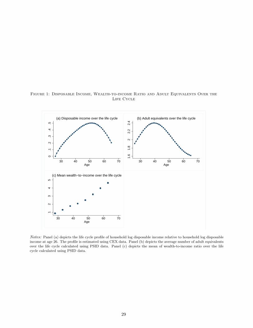
Figure 1: Disposable Income, Wealth-to-income Ratio and Adult Equivalents Over theLife Cycle
0.1
.2.3
.4.5
30 40 50 60 70Age
(a) Disposable income over the life cycle
1.6
1.8
22.
22.
4
30 40 50 60 70Age
(b) Adult equivalents over the life cycle
12
34
5
30 40 50 60 70Age
(c) Mean wealth−to−income over the life cycle
Notes: Panel (a) depicts the life cycle profile of household log disposable income relative to household log disposableincome at age 26. The profile is estimated using CEX data. Panel (b) depicts the average number of adult equivalentsover the life cycle calculated using PSID data. Panel (c) depicts the mean of wealth-to-income ratio over the lifecycle calculated using PSID data.
29
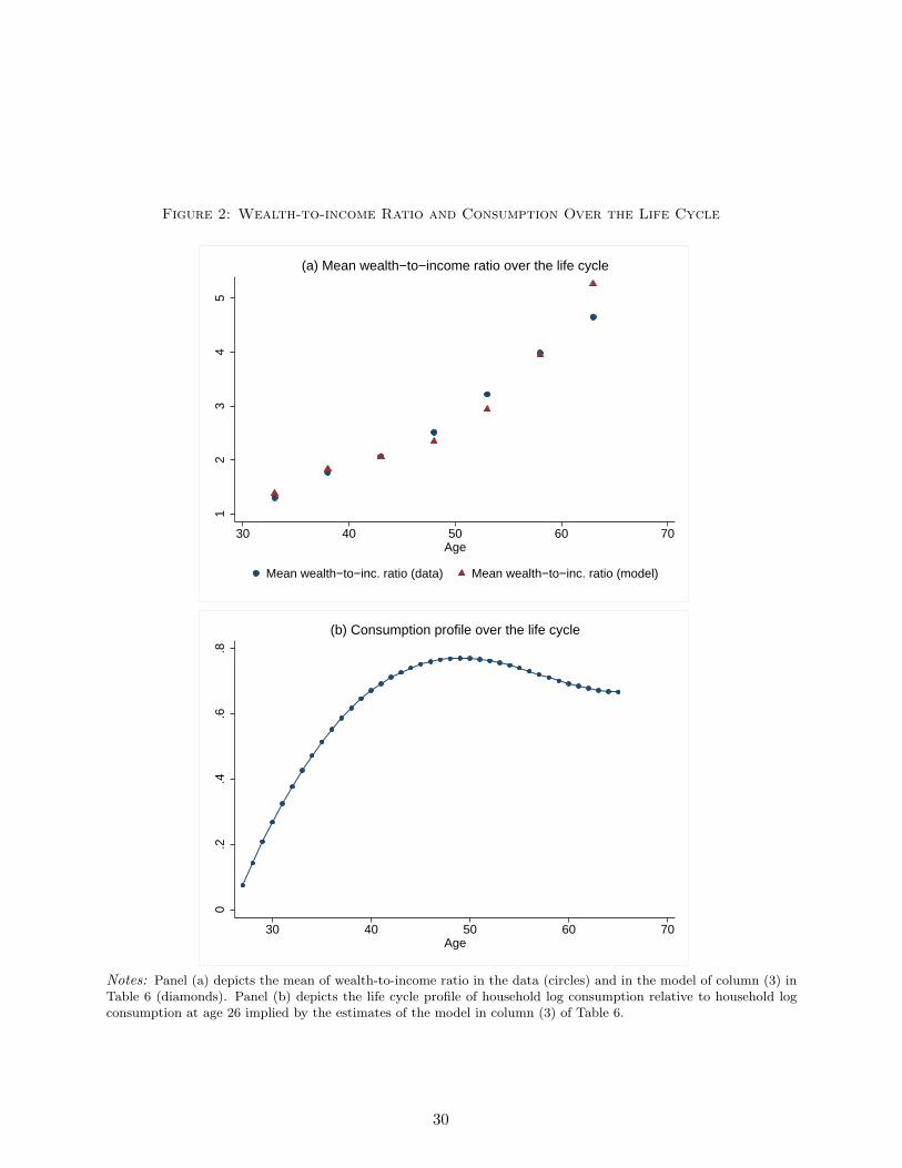
Figure 2: Wealth-to-income Ratio and Consumption Over the Life Cycle1
23
45
30 40 50 60 70Age
Mean wealth−to−inc. ratio (data) Mean wealth−to−inc. ratio (model)
(a) Mean wealth−to−income ratio over the life cycle
0.2
.4.6
.8
30 40 50 60 70Age
(b) Consumption profile over the life cycle
Notes: Panel (a) depicts the mean of wealth-to-income ratio in the data (circles) and in the model of column (3) inTable 6 (diamonds). Panel (b) depicts the life cycle profile of household log consumption relative to household logconsumption at age 26 implied by the estimates of the model in column (3) of Table 6.
30
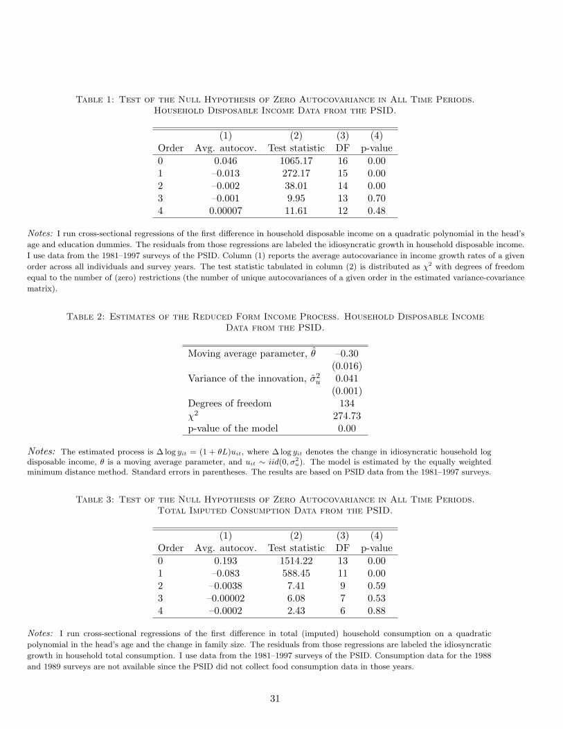
Table 1: Test of the Null Hypothesis of Zero Autocovariance in All Time Periods.Household Disposable Income Data from the PSID.
(1) (2) (3) (4)Order Avg. autocov. Test statistic DF p-value
0 0.046 1065.17 16 0.001 –0.013 272.17 15 0.002 –0.002 38.01 14 0.003 –0.001 9.95 13 0.704 0.00007 11.61 12 0.48
Notes: I run cross-sectional regressions of the first difference in household disposable income on a quadratic polynomial in the head’s
age and education dummies. The residuals from those regressions are labeled the idiosyncratic growth in household disposable income.
I use data from the 1981–1997 surveys of the PSID. Column (1) reports the average autocovariance in income growth rates of a given
order across all individuals and survey years. The test statistic tabulated in column (2) is distributed as χ2 with degrees of freedom
equal to the number of (zero) restrictions (the number of unique autocovariances of a given order in the estimated variance-covariance
matrix).
Table 2: Estimates of the Reduced Form Income Process. Household Disposable IncomeData from the PSID.
Moving average parameter, θ –0.30(0.016)
Variance of the innovation, σ2u 0.041
(0.001)Degrees of freedom 134χ2 274.73p-value of the model 0.00
Notes: The estimated process is ∆ log yit = (1 + θL)uit, where ∆ log yit denotes the change in idiosyncratic household logdisposable income, θ is a moving average parameter, and uit ∼ iid(0, σ2
u). The model is estimated by the equally weightedminimum distance method. Standard errors in parentheses. The results are based on PSID data from the 1981–1997 surveys.
Table 3: Test of the Null Hypothesis of Zero Autocovariance in All Time Periods.Total Imputed Consumption Data from the PSID.
(1) (2) (3) (4)Order Avg. autocov. Test statistic DF p-value
0 0.193 1514.22 13 0.001 –0.083 588.45 11 0.002 –0.0038 7.41 9 0.593 –0.00002 6.08 7 0.534 –0.0002 2.43 6 0.88
Notes: I run cross-sectional regressions of the first difference in total (imputed) household consumption on a quadratic
polynomial in the head’s age and the change in family size. The residuals from those regressions are labeled the idiosyncratic
growth in household total consumption. I use data from the 1981–1997 surveys of the PSID. Consumption data for the 1988
and 1989 surveys are not available since the PSID did not collect food consumption data in those years.
31
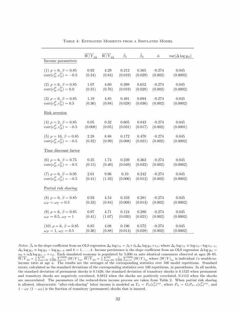
Table 4: Estimated Moments from a Simulated Model
W/Y 33 W/Y 63 β1 β4 α var(∆ log yit)Income parameters
(1) ρ = 6, β = 0.85 0.92 4.29 0.212 0.565 –0.274 0.045corr(ϵPit, ϵ
Tit) = −0.5 (0.34) (0.84) (0.019) (0.029) (0.002) (0.0002)
(2) ρ = 6, β = 0.85 1.07 4.60 0.398 0.652 –0.274 0.045corr(ϵPit, ϵ
Tit) = 0.0 (0.31) (0.76) (0.019) (0.028) (0.002) (0.0002)
(3) ρ = 6, β = 0.85 1.19 4.85 0.491 0.694 –0.274 0.045corr(ϵPit, ϵ
Tit) = 0.5 (0.36) (0.88) (0.028) (0.036) (0.002) (0.0002)
Risk aversion
(4) ρ = 2, β = 0.85 0.05 0.32 0.605 0.843 –0.274 0.045corr(ϵPit, ϵ
Tit) = −0.5 (0.008) (0.05) (0.031) (0.017) (0.002) (0.0001)
(5) ρ = 10, β = 0.85 2.28 8.88 0.172 0.470 –0.274 0.045corr(ϵPit, ϵ
Tit) = −0.5 (0.32) (0.99) (0.008) (0.021) (0.002) (0.0002)
Time discount factor
(6) ρ = 6, β = 0.75 0.25 1.74 0.239 0.363 –0.274 0.045corr(ϵPit, ϵ
Tit) = −0.5 (0.15) (0.40) (0.049) (0.032) (0.002) (0.0002)
(7) ρ = 6, β = 0.95 2.01 9.96 0.10 0.242 –0.274 0.045corr(ϵPit, ϵ
Tit) = −0.5 (0.41) (1.33) (0.006) (0.012) (0.002) (0.0002)
Partial risk sharing
(8) ρ = 6, β = 0.85 0.93 4.54 0.103 0.281 –0.274 0.045ωP = ωT = 0.5 (0.33) (0.84) (0.008) (0.013) (0.002) (0.0002)
(9) ρ = 6, β = 0.85 0.97 4.71 0.124 0.280 –0.274 0.045ωP = 0.5, ωT = 1 (0.41) (1.07) (0.020) (0.021) (0.002) (0.0002)
(10) ρ = 6, β = 0.85 0.85 4.08 0.196 0.572 –0.274 0.045ωP = 1, ωT = 0.5 (0.36) (0.88) (0.014) (0.028) (0.002) (0.0002)
Notes: βk is the slope coefficient from an OLS regression ∆k log cit = β0+βk∆k log yit+ϵit; where ∆k log cit ≡ log cit−log cit−k,∆k log yit ≡ log yit − log yit−k and k = 1, . . . , 4. Income persistence is the slope coefficient from an OLS regression ∆ log yit =α0 + α∆log yit−1 + ϵit. Each simulated economy is populated by 5,000 ex ante identical consumers observed at ages 26–65.W/Y 33 = 1
5
∑35a=31
15,000
∑5000i=1 (W/Y )ia, W/Y 63 = 1
5
∑65a=61
15,000
∑5000i=1 (W/Y )ia where (W/Y )ia is individual i’s wealth-to-
income ratio at age a. The results are the averages of the corresponding statistics over 100 model repetitions. Standarderrors, calculated as the standard deviations of the corresponding statistics over 100 repetitions, in parentheses. In all models,the standard deviation of permanent shocks is 0.1426; the standard deviation of transitory shocks is 0.1525 when permanentand transitory shocks are negatively correlated, 0.0812 when the shocks are positively correlated, 0.1112 when the shocksare uncorrelated. The parameters of the reduced-form income process are taken from Table 2. When partial risk sharingis allowed, idiosyncratic “after-risk-sharing” labor income is modeled as Yit = Pit(ϵ
Tit)
ωT , where Pit = GtPit−1(ϵPit)
ωP , and1− ωT (1− ωP ) is the fraction of transitory (permanent) shocks that is insured.
32
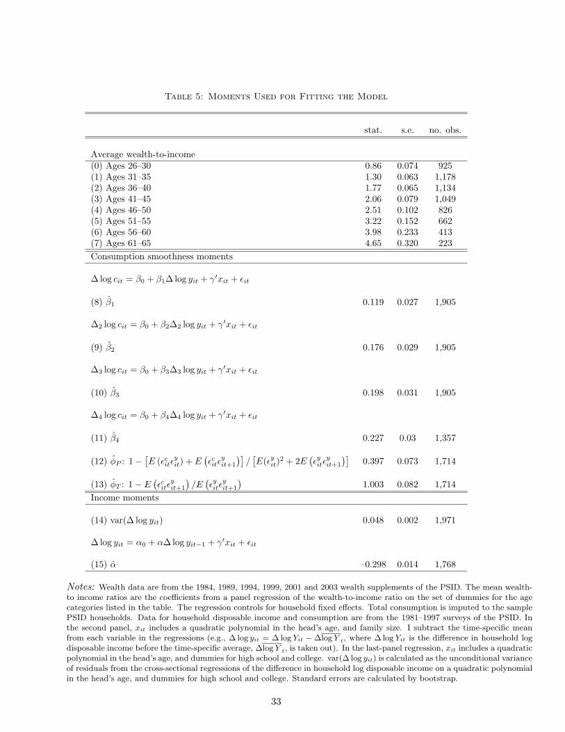
Table 5: Moments Used for Fitting the Model
stat. s.e. no. obs.
Average wealth-to-income(0) Ages 26–30 0.86 0.074 925(1) Ages 31–35 1.30 0.063 1,178(2) Ages 36–40 1.77 0.065 1,134(3) Ages 41–45 2.06 0.079 1,049(4) Ages 46–50 2.51 0.102 826(5) Ages 51–55 3.22 0.152 662(6) Ages 56–60 3.98 0.233 413(7) Ages 61–65 4.65 0.320 223
Consumption smoothness moments
∆ log cit = β0 + β1∆log yit + γ′xit + ϵit
(8) β1 0.119 0.027 1,905
∆2 log cit = β0 + β2∆2 log yit + γ′xit + ϵit
(9) β2 0.176 0.029 1,905
∆3 log cit = β0 + β3∆3 log yit + γ′xit + ϵit
(10) β3 0.198 0.031 1,905
∆4 log cit = β0 + β4∆4 log yit + γ′xit + ϵit
(11) β4 0.227 0.03 1,357
(12) ϕP : 1−[E (ϵcitϵ
yit) + E
(ϵcitϵ
yit+1
)]/[E(ϵyit)
2 + 2E(ϵyitϵ
yit+1
)]0.397 0.073 1,714
(13) ϕT : 1− E(ϵcitϵ
yit+1
)/E
(ϵyitϵ
yit+1
)1.003 0.082 1,714
Income moments
(14) var(∆ log yit) 0.048 0.002 1,971
∆ log yit = α0 + α∆log yit−1 + γ′xit + ϵit
(15) α –0.298 0.014 1,768
Notes: Wealth data are from the 1984, 1989, 1994, 1999, 2001 and 2003 wealth supplements of the PSID. The mean wealth-to income ratios are the coefficients from a panel regression of the wealth-to-income ratio on the set of dummies for the agecategories listed in the table. The regression controls for household fixed effects. Total consumption is imputed to the samplePSID households. Data for household disposable income and consumption are from the 1981–1997 surveys of the PSID. Inthe second panel, xit includes a quadratic polynomial in the head’s age, and family size. I subtract the time-specific meanfrom each variable in the regressions (e.g., ∆ log yit = ∆ log Yit − ∆log Y t, where ∆ log Yit is the difference in household logdisposable income before the time-specific average, ∆log Y t, is taken out). In the last-panel regression, xit includes a quadraticpolynomial in the head’s age, and dummies for high school and college. var(∆ log yit) is calculated as the unconditional varianceof residuals from the cross-sectional regressions of the difference in household log disposable income on a quadratic polynomialin the head’s age, and dummies for high school and college. Standard errors are calculated by bootstrap.
33
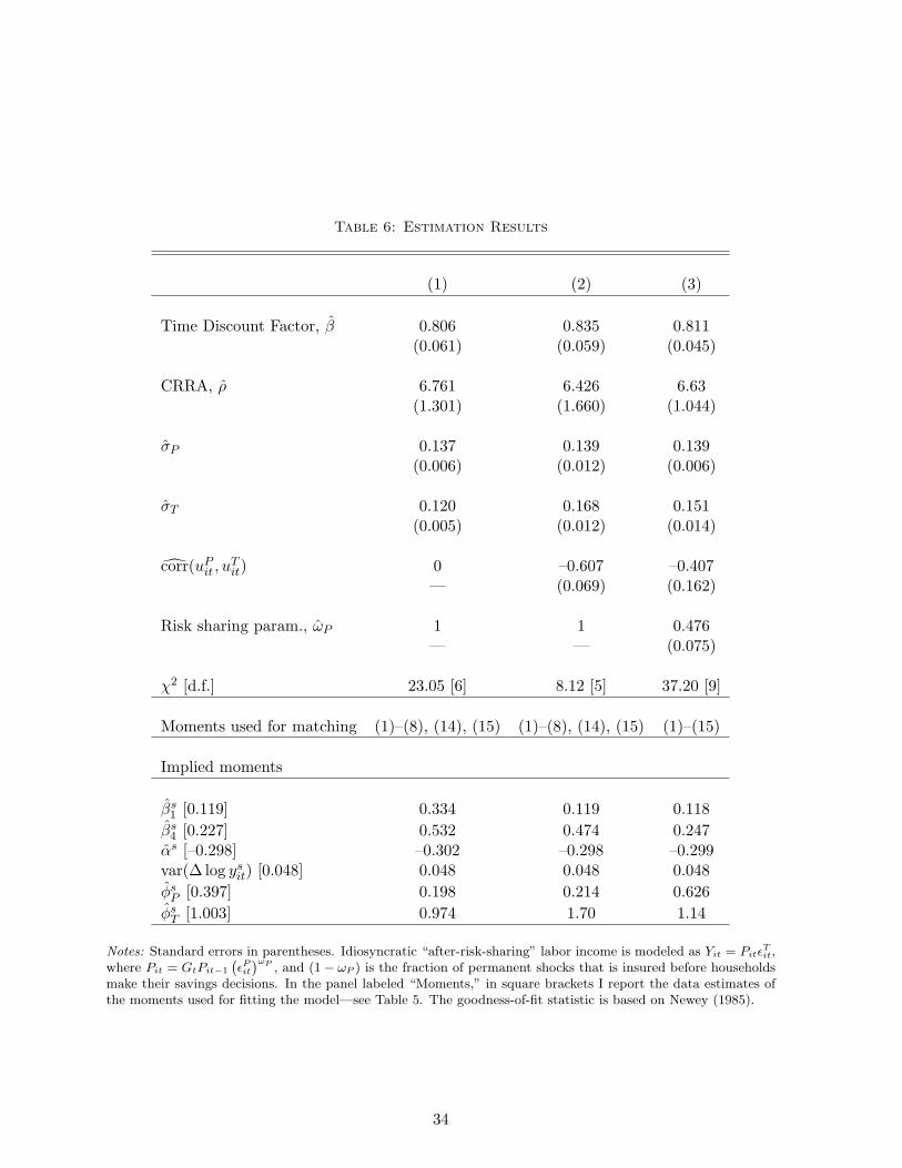
Table 6: Estimation Results
(1) (2) (3)
Time Discount Factor, β 0.806 0.835 0.811(0.061) (0.059) (0.045)
CRRA, ρ 6.761 6.426 6.63(1.301) (1.660) (1.044)
σP 0.137 0.139 0.139(0.006) (0.012) (0.006)
σT 0.120 0.168 0.151(0.005) (0.012) (0.014)
corr(uPit , uTit) 0 –0.607 –0.407
— (0.069) (0.162)
Risk sharing param., ωP 1 1 0.476— — (0.075)
χ2 [d.f.] 23.05 [6] 8.12 [5] 37.20 [9]
Moments used for matching (1)–(8), (14), (15) (1)–(8), (14), (15) (1)–(15)
Implied moments
βs1 [0.119] 0.334 0.119 0.118
βs4 [0.227] 0.532 0.474 0.247
αs [–0.298] –0.302 –0.298 –0.299var(∆ log ysit) [0.048] 0.048 0.048 0.048
ϕsP [0.397] 0.198 0.214 0.626
ϕsT [1.003] 0.974 1.70 1.14
Notes: Standard errors in parentheses. Idiosyncratic “after-risk-sharing” labor income is modeled as Yit = PitϵTit,
where Pit = GtPit−1
(ϵPit
)ωP , and (1− ωP ) is the fraction of permanent shocks that is insured before householdsmake their savings decisions. In the panel labeled “Moments,” in square brackets I report the data estimates ofthe moments used for fitting the model—see Table 5. The goodness-of-fit statistic is based on Newey (1985).
34
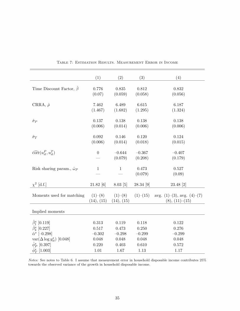
Table 7: Estimation Results. Measurement Error in Income
(1) (2) (3) (4)
Time Discount Factor, β 0.776 0.835 0.812 0.832(0.07) (0.059) (0.058) (0.056)
CRRA, ρ 7.462 6.489 6.615 6.187(1.467) (1.682) (1.295) (1.324)
σP 0.137 0.138 0.138 0.138(0.006) (0.014) (0.006) (0.006)
σT 0.092 0.146 0.120 0.124(0.006) (0.014) (0.018) (0.015)
corr(uPit , uTit) 0 –0.644 –0.367 –0.407
— (0.079) (0.208) (0.179)
Risk sharing param., ωP 1 1 0.473 0.527— — (0.079) (0.09)
χ2 [d.f.] 21.82 [6] 8.03 [5] 28.34 [9] 23.48 [2]
Moments used for matching (1)–(8) (1)–(8) (1)–(15) avg. (1)–(3), avg. (4)–(7)(14), (15) (14), (15) (8), (11)–(15)
Implied moments
βs1 [0.119] 0.313 0.119 0.118 0.122
βs4 [0.227] 0.517 0.473 0.250 0.276
αs [–0.298] –0.302 –0.298 –0.299 –0.299var(∆ log ysit) [0.048] 0.048 0.048 0.048 0.048
ϕsP [0.397] 0.220 0.403 0.610 0.572
ϕsT [1.003] 1.01 1.67 1.13 1.17
Notes: See notes to Table 6. I assume that measurement error in household disposable income contributes 25%towards the observed variance of the growth in household disposable income.
35

Appendix A. Matching the Moments of the Reduced Form andStructural Income Models
As in the text, suppose that the first difference of log income is described by the reduced form MA(1)process. Thus, the unique moments of the reduced form (rf) are the first and zero-order autocovariances:
γrf (0) = (1 + θ2)σ2u,
γrf (1) = θσ2u.
For a structural model (sf) with correlated permanent and transitory components described in thetext, I need to match
γsf (0) = σ2uP + 2σ2
uT + 2cov(uPit, u
Tit) = γrf (0),
γsf (1) = −σ2uT − cov(uP
it, uTit) = γrf (1),
subject to the constraint that the spectrum of the reduced form series and the permanent component atfrequency zero are equal:
σ2uP = γrf (0) + 2γrf (1) = (1 + θ)2σ2
u.
The above equation is the identifying condition for the variance of the permanent component. The twopreceding equations determine the other two unknowns, cov(uP
it, uTit) and σuT . Since the two equations
have three unknowns, there is no unique solution for cov(uPit, u
Tit) and σuT . Thus, I choose the grid of
covariances between the shocks such that they return the correlation that is less than or equal to one inabsolute value. This procedure uniquely determines the variance of the transitory innovation from thefollowing condition:
σ2uT = −γrf (1)− cov(uP
it, uTit).
The estimated parameters of the reduced form process for the growth in idiosyncratic income arein Table 2. The structural income processes are of the form: ∆ log yit = uP
it + ∆uTit, with potentially
correlated permanent and transitory shocks.
Appendix B. Numerical Procedures
In this appendix, I lay out the details of model solution, and describe the choices made in numericalanalysis.
Model SolutionAt age 90, the last period of the problem, CT = XT , where CT andXT are household consumption and
cash-on-hand at age T , respectively. At each age of the life cycle, the Euler equation linking consumption
in adjacent periods is ntu′(
Ct
nt
)= βRnt+1Etu
′(
Ct+1[R(Xt−Ct)+Yt+1]nt+1
), where expectation is taken with
respect to future mortality risk at ages 65, . . . , 89 and labor income risk at ages 26, . . . , 64. Given thatCt+1(Xt+1) is known, the Euler equation provides the unique solution for Ct given Xt. I express theproblem in terms of consumption and cash-on-hand relative to the permanent component of income (ctand xt, respectively).
I solve the problem using the endogenous gridpoints method in Carroll (2006). I create a grid of120 points in st = xt − ct, and a 250 × 2 matrix of pre-seeded independent random normal deviates ϵ1,
36
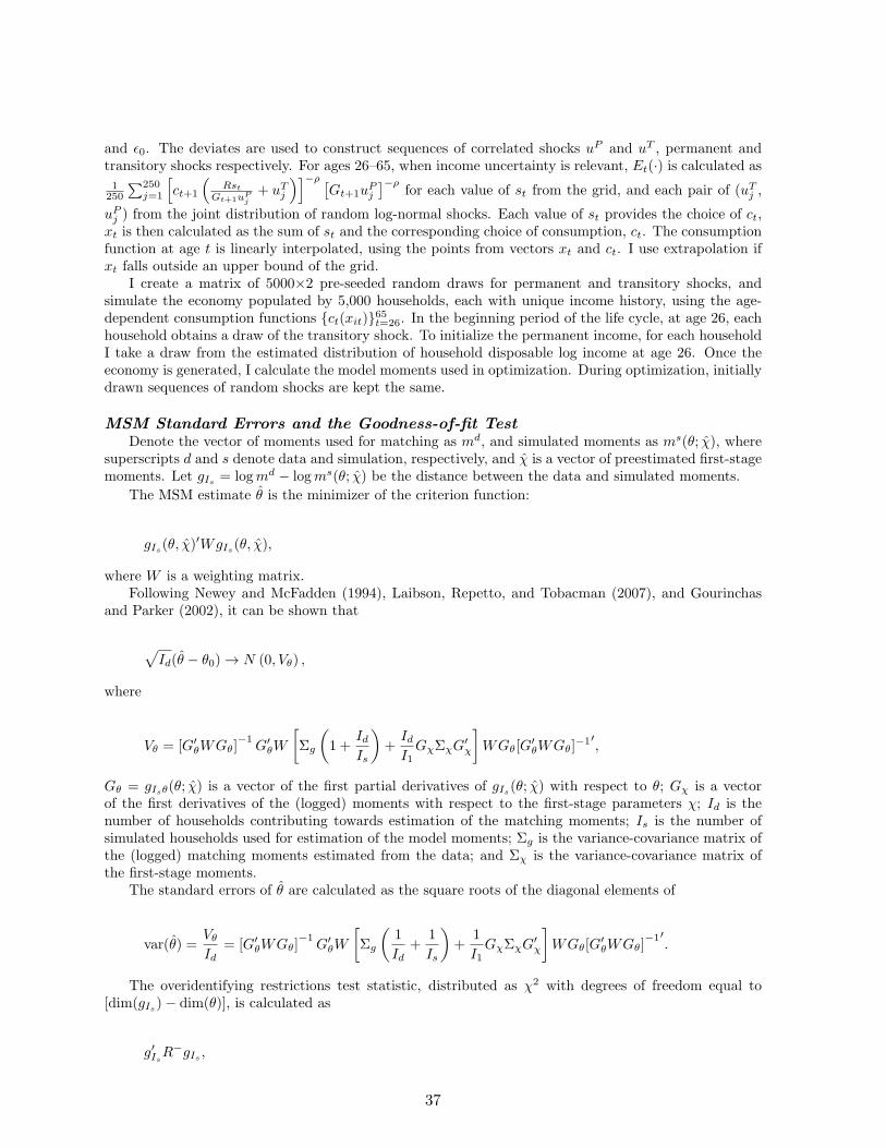
and ϵ0. The deviates are used to construct sequences of correlated shocks uP and uT , permanent andtransitory shocks respectively. For ages 26–65, when income uncertainty is relevant, Et(·) is calculated as
1250
∑250j=1
[ct+1
(Rst
Gt+1uPj+ uT
j
)]−ρ [Gt+1u
Pj
]−ρfor each value of st from the grid, and each pair of (uT
j ,
uPj ) from the joint distribution of random log-normal shocks. Each value of st provides the choice of ct,
xt is then calculated as the sum of st and the corresponding choice of consumption, ct. The consumptionfunction at age t is linearly interpolated, using the points from vectors xt and ct. I use extrapolation ifxt falls outside an upper bound of the grid.
I create a matrix of 5000×2 pre-seeded random draws for permanent and transitory shocks, andsimulate the economy populated by 5,000 households, each with unique income history, using the age-dependent consumption functions ct(xit)65t=26. In the beginning period of the life cycle, at age 26, eachhousehold obtains a draw of the transitory shock. To initialize the permanent income, for each householdI take a draw from the estimated distribution of household disposable log income at age 26. Once theeconomy is generated, I calculate the model moments used in optimization. During optimization, initiallydrawn sequences of random shocks are kept the same.
MSM Standard Errors and the Goodness-of-fit TestDenote the vector of moments used for matching as md, and simulated moments as ms(θ; χ), where
superscripts d and s denote data and simulation, respectively, and χ is a vector of preestimated first-stagemoments. Let gIs = logmd − logms(θ; χ) be the distance between the data and simulated moments.
The MSM estimate θ is the minimizer of the criterion function:
gIs(θ, χ)′WgIs(θ, χ),
where W is a weighting matrix.Following Newey and McFadden (1994), Laibson, Repetto, and Tobacman (2007), and Gourinchas
and Parker (2002), it can be shown that
√Id(θ − θ0) → N (0, Vθ) ,
where
Vθ = [G′θWGθ]
−1G′
θW
[Σg
(1 +
IdIs
)+
IdI1
GχΣχG′χ
]WGθ[G
′θWGθ]
−1′,
Gθ = gIsθ(θ; χ) is a vector of the first partial derivatives of gIs(θ; χ) with respect to θ; Gχ is a vectorof the first derivatives of the (logged) moments with respect to the first-stage parameters χ; Id is thenumber of households contributing towards estimation of the matching moments; Is is the number ofsimulated households used for estimation of the model moments; Σg is the variance-covariance matrix ofthe (logged) matching moments estimated from the data; and Σχ is the variance-covariance matrix ofthe first-stage moments.
The standard errors of θ are calculated as the square roots of the diagonal elements of
var(θ) =Vθ
Id= [G′
θWGθ]−1
G′θW
[Σg
(1
Id+
1
Is
)+
1
I1GχΣχG
′χ
]WGθ[G
′θWGθ]
−1′.
The overidentifying restrictions test statistic, distributed as χ2 with degrees of freedom equal to[dim(gIs)− dim(θ)], is calculated as
g′IsR−gIs ,
37
where R− is a generalized inverse (calculated as the Moore-Penrose inverse) of the matrix R = P Vθ
IdP ′,
P = I −Gθ(G′θWGθ)G
′θW (see Newey 1985).
Appendix C. Data Used and Sample Selection
The Consumer Expenditure SurveyI use CEX data on total consumer expenditures and food consumption, available at the NBER website.
The data set spans the period 1980–2003. The CEX is designed by the Bureau of Labor Statistics toconstruct the CPI at different levels of aggregation. The survey publishes at most four quarters ofinformation on individual consumption, along with demographic information. The NBER extracts lumpquarterly records into one annual record.
Total consumption is defined as household total expenditures on nondurables (food at home, foodat work, food away from home, clothes, personal care items, utility payments, transportation includinggasoline and insurance, recreation services, gambling and charity), household supplies and equipment,rents, medical services, vehicles and auto parts, books and publications, education, interest payments,housing property taxes, contributions to private pensions and self-employed retirement. The measure isdefined similarly to Blundell, Pistaferri, and Preston (2008).
Households may enter the survey in the same year but in different quarters and months of a quarter.If household consumption record relates both to years t and t+1, I assume that annual consumption refersto year t if that year contains at least six months of consumption records, and to year t + 1 otherwise.In the CEX, the head of a household is the person who owns or rents the unit of household residence. Inthe PSID, the head of a household is male, unless he is permanently disabled (see Hill 1992). To makethe definitions of heads comparable, I assume that heads are males in the CEX families with couples.
My sample selection steps are the following. First, I keep only the households that report expendituresin all four quarters of the year, and who are classified as full income reporters. I further keep marriedcouples, with heads who are not self-employed, of age above 25 but below 71; and with family sizeequal or greater than 2 family members. I drop households whose heads attend college, part-time orfull-time; or do not have education, race, age, or state of residence records. I also drop households thatreport zero expenditures on food at home. I deflate food at home, food away from home, total foodas well as total household expenditures by the Bureau of Labor Statistics (BLS) food at home, foodaway, total food and all items CPI with the base 100 in 1982–1984, respectively. I use non-seasonallyadjusted, U.S. city average CPI indices for March of the respective year. I further drop households whoseexpenditures on food at home and away from home exceed household disposable income. Householddisposable income is defined as the difference between household taxable income and federal incometaxes. Household taxable income, in turn, is the sum of wages and salaries, rents, dividends and interest,business and farm income, pensions, social security benefits, supplemental security income, unemploymentcompensation, and workers’ compensation for all family members. To eliminate the influence of outliers,I drop observations below the 1st and above the 99th percentiles of the annual total food distributions.
I utilize information on 23,133 households whose heads are of ages 26–65 to estimate the relationshipbetween food consumption and total consumption. The relationship is later used for imputation of thetotal consumption to the sample PSID households. I use income information for households whose headsare of ages 26–70 to estimate the deterministic profile of life-cycle growth in household disposable income.
The Panel Study of Income DynamicsI use PSID data from the 1981–2003 waves, the same time span during which I have data on consump-
tion and demographics in the CEX. To allow for a more representative sample, I drop households thatare part of the Survey of Economic Opportunity (SEO) subsample. The PSID consistently collected onlytwo items of consumption over time: food consumption at home and food consumption away from home(excluding food at work). Since I am interested in total household consumption and income dynamicsover the life cycle, I impute total consumption to the PSID households. Most of the studies that use foodconsumption from the PSID assume that food consumption recorded in survey year t reflects the typicalweekly food consumption flow in year t−1. In this paper, I adopt the same strategy. Over the time span
38
considered, the PSID did not collect food consumption data in 1988 and 1989. Correspondingly, my finalsample of analysis lacks food and total consumption data for 1987 and 1988. Food away from home andfood at home are deflated by their respective CPIs taken from the BLS.
The sample selection details are as follows. I first make the age series consistent throughout thesurvey years. An individual’s age in adjacent years can be the same or differ by more than one yearsince households may be interviewed in different months of a year. I take the first record on age when anindividual appears as the head of household and impute age in other years using that record. I then drophouseholds whose heads are younger than 26 or older than 70, and all female-headed households. I thenchoose continuously married heads with the longest spell of an uninterrupted headship. I further drophouseholds whose heads had a spell of self-employment, and keep those who never experienced significantchanges in family composition, that is those who had no changes at all or changes in members other thanthe head or wife. I drop households with inconsistent race records (e.g., households whose heads reportbeing white in one survey year and black in some other year), and households with heads who becomepermanently disabled or continue schooling after age 26. I set head’s education to the maximum yearsof schooling reported by the head during sample years. Heads are then assigned to three educationalcategories: high school dropouts (with years of schooling below 12), high school graduates (with yearsof schooling above 11 but less than 16 years), and college graduates (with years of schooling equal to orexceeding 16 years). I further drop observations with missing records on head’s or household disposableincome; with zero records on head’s income when heads are of ages 26 to 65, at their pre-retirementstage of the life cycle. I also drop income outliers and single-headed households. An income outlier isdefined as an observation on household disposable income at time t when the growth rate in householddisposable income between periods t− 1 and t is above 500 percent or below –80 percent. I then select,for each household, the longest spell of an uninterrupted headship with all relevant information. I keepthose who were born between 1912 and 1978, and whose total food expenditures do not exceed householddisposable income. I also drop observations with household food expenditures above the 99th or belowthe 1st percentiles of the annual food distributions. Similar to my selection rules for the CEX sample,I drop observations with expenditures on food at home equal to zero. In the PSID, income recordedin year t refers to income earned in year t − 1. Conformably with income observations, I assume thatdemographic information and household food expenditures recorded in year t refer to a previous year.
Before 1994, the PSID recorded annual household expenditures on food at home or away from home.In 1994, the PSID started recording food at home and food away from home at different frequencies—daily, weekly, biweekly, monthly, or annual frequency. For those years, I use household food records atthe monthly or weekly frequency. I lose a small number of observations on household food expendituresreported at other frequencies. Most of them, when converted to annual amounts, were clear outliers.
The PSID estimated household federal income taxes for 1980–1991. Starting in 1992, the PSIDdiscontinued calculation of federal income taxes. Since my data extend well beyond 1992, I use theTAXSIM tool at the NBER to calculate a consistent series of household federal income taxes and socialsecurity withholdings. I assume that family members other than the head and wife are filing their taxreturns separately. Household disposable income is then calculated as the sum of the head’s and wife’slabor income, their combined transfer income, transfer income of all other family members, taxableincome of other family members less federal income taxes and social security withholdings for the headand wife and all other family members. I also add the total family social security income for 1994–2003to the measure of disposable income since the records on head’s and wife’s transfer income and transferincome of other family members exclude social security income in those years.
For the households in my final sample, I use wealth information from the 1984, 1989, 1994, 1999, 2001and 2003 wealth supplements. The wealth measure utilized is the total household net worth exclusive ofhousehold business wealth.
Imputation of ConsumptionIn this appendix, I describe the procedure used to impute total consumption to the PSID households.
Absent data on total consumption in the PSID, imputation is usually done in order to exploit the panelstructure of the PSID. Skinner (1987), using the 1972–1973 and 1983 waves of the CEX, showed thattotal household consumption tightly relates to several consumption items, also available in the PSID
39

(food at home and away from home, number of vehicles owned, and housing rent). Moreover, he showedthat this relationship is stable over time. Blundell, Pistaferri, and Preston (2005) pioneered a structuralapproach to imputation—inverting the food demand equation estimated on CEX data. They relate foodconsumption to nondurable expenditures, household demographics, price indices, time dummies, cohortdummies, and nondurable expenditures interacted with time dummies and the head’s education category.I run a similar regression, and use the coefficients from this regression to impute total consumption tothe PSID households. In the OLS setting, the estimated elasticities may be biased due to measurementerror in total expenditures, and endogeneity of food and total consumption. I therefore follow Blundell,Pistaferri, and Preston (2008), and instrument log total expenditures (and its interactions with yearand education dummies) with the head’s and wife’s education-year-cohort specific averages of log hourlywages (and their interactions with year and education dummies). The results of an IV regression offood consumption on total expenditures are presented in Table C-1. The estimated elasticity of foodconsumption with respect to total expenditures is high in the 1980s, and drops steadily to about 0.60 in2002.
40
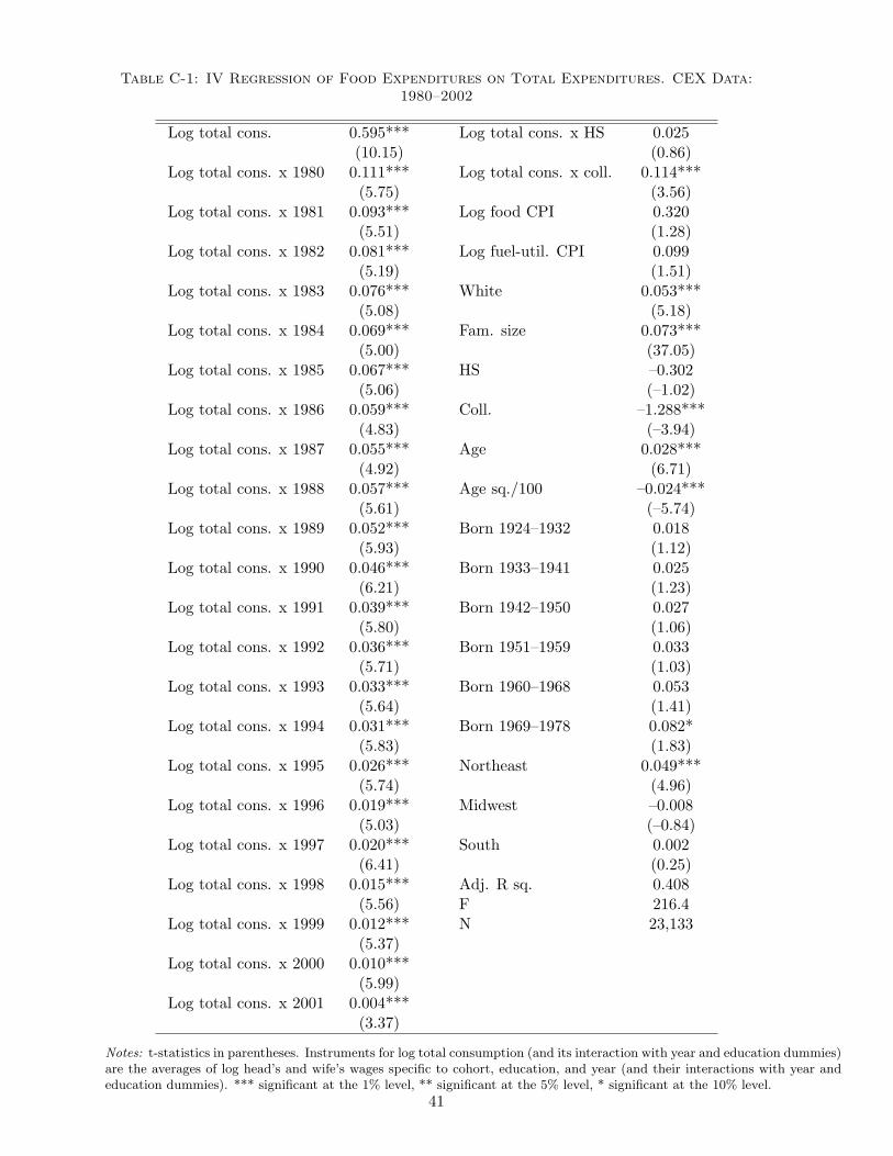
Table C-1: IV Regression of Food Expenditures on Total Expenditures. CEX Data:1980–2002
Log total cons. 0.595*** Log total cons. x HS 0.025(10.15) (0.86)
Log total cons. x 1980 0.111*** Log total cons. x coll. 0.114***(5.75) (3.56)
Log total cons. x 1981 0.093*** Log food CPI 0.320(5.51) (1.28)
Log total cons. x 1982 0.081*** Log fuel-util. CPI 0.099(5.19) (1.51)
Log total cons. x 1983 0.076*** White 0.053***(5.08) (5.18)
Log total cons. x 1984 0.069*** Fam. size 0.073***(5.00) (37.05)
Log total cons. x 1985 0.067*** HS –0.302(5.06) (–1.02)
Log total cons. x 1986 0.059*** Coll. –1.288***(4.83) (–3.94)
Log total cons. x 1987 0.055*** Age 0.028***(4.92) (6.71)
Log total cons. x 1988 0.057*** Age sq./100 –0.024***(5.61) (–5.74)
Log total cons. x 1989 0.052*** Born 1924–1932 0.018(5.93) (1.12)
Log total cons. x 1990 0.046*** Born 1933–1941 0.025(6.21) (1.23)
Log total cons. x 1991 0.039*** Born 1942–1950 0.027(5.80) (1.06)
Log total cons. x 1992 0.036*** Born 1951–1959 0.033(5.71) (1.03)
Log total cons. x 1993 0.033*** Born 1960–1968 0.053(5.64) (1.41)
Log total cons. x 1994 0.031*** Born 1969–1978 0.082*(5.83) (1.83)
Log total cons. x 1995 0.026*** Northeast 0.049***(5.74) (4.96)
Log total cons. x 1996 0.019*** Midwest –0.008(5.03) (–0.84)
Log total cons. x 1997 0.020*** South 0.002(6.41) (0.25)
Log total cons. x 1998 0.015*** Adj. R sq. 0.408(5.56) F 216.4
Log total cons. x 1999 0.012*** N 23,133(5.37)
Log total cons. x 2000 0.010***(5.99)
Log total cons. x 2001 0.004***(3.37)
Notes: t-statistics in parentheses. Instruments for log total consumption (and its interaction with year and education dummies)are the averages of log head’s and wife’s wages specific to cohort, education, and year (and their interactions with year andeducation dummies). *** significant at the 1% level, ** significant at the 5% level, * significant at the 10% level.
41