Excel tips & tricks This pdf contains “good to know” tips and tricks about Microsoft Excel . They are structured in step by

step tutorials so you can easily follow along.

There are also short introductions to the most important featues in Excel like pivot tables, vba

macros, conditional formatting, data validation, excel tables.

On the next page you will find table of contents. It will help you navigate this pdf.

Table of Contents

1 Learn Pivot table basics ................................................................................................................... 4

2 Conditional formatting .................................................................................................................... 8

2.1 Conditional formatting – formula .......................................................................................... 10

3 Sort & Filter ................................................................................................................................... 12

4 Data Validation .............................................................................................................................. 14

4.1 Data Validation ...................................................................................................................... 14

4.2 Data Validation – Prevent duplicate records ......................................................................... 16

5 Excel defined tables ....................................................................................................................... 18

5.1 Quickly create an Excel defined table .................................................................................... 18

5.2 Dynamic charts – excel defined table .................................................................................... 19

6 Excel named ranges ....................................................................................................................... 20

6.1 How to use the name manager ............................................................................................. 20

6.2 Quickly open the name manager (keyboard shortcut) ......................................................... 22

6.3 Show named ranges .............................................................................................................. 23

6.4 Quickly create a named range ............................................................................................... 24

7 Dynamic named ranges ................................................................................................................. 25

8 Visual basic for applications .......................................................................................................... 27

8.1 Enable Developer tab on the ribbon ..................................................................................... 27

8.2 Macro recorder – learn vba ................................................................................................... 28

8.3 Quickly open VB Editor using a keyboard shortcut ............................................................... 29

8.4 Assign a macro to a button .................................................................................................... 30

9 Keyboard shortcuts ........................................................................................................................ 31

9.1 Press Alt key to see available keyboard short cuts ................................................................ 31

9.2 Shortcut keys to quickly enter todays date in a cell .............................................................. 32

9.3 Short cut keys to enter current time in a cell ........................................................................ 33

9.4 Keyboard Short cut -Jump to next empty cell ....................................................................... 34

9.5 Quickly select a data range .................................................................................................... 35

9.6 Select the entire column or row ............................................................................................ 36

9.7 Important keyboard shortcuts in excel .................................................................................. 37

10 Quickly format a cell .................................................................................................................. 38

11 Excel formulas ............................................................................................................................ 39

11.1 Evaluate formula .................................................................................................................... 39

11.2 Change relative cell ref to absolute cell ref ........................................................................... 40

11.3 Convert cell reference to values ............................................................................................ 42

11.4 Enter a value or a formula in empty cells .............................................................................. 43

11.5 Use INDEX + MATCH instead of VLOOKUP ............................................................................. 45

11.6 Concatenate cell values ......................................................................................................... 46

11.7 Autosum ................................................................................................................................ 47

11.8 Copy formula and paste value ............................................................................................... 48

12 Transpose values in a column to a row ...................................................................................... 49

13 Transpose a table ....................................................................................................................... 50

14 Formatting ................................................................................................................................. 51

14.1 Highlight every second row in a data set ............................................................................... 51

14.2 Hide values in a sheet ............................................................................................................ 53

14.3 Quickly format a cell or a cell range ...................................................................................... 55

14.4 Double click format painter to copy and paste formats to other cells .................................. 56

14.5 Create a hyperlink .................................................................................................................. 57

15 Working with cells ..................................................................................................................... 59

15.1 Edit a cell ............................................................................................................................... 59

15.2 How to quickly change multiple column or row widths on a sheet ...................................... 60

15.3 Quickly hide and unhide a column or a row using a keyboard shortcut ............................... 61

15.4 Undo, redo or repeat command (keyboard shortcuts) ......................................................... 62

15.5 Quickly select all cells with comments .................................................................................. 63

15.6 Copy | Paste | Cut ................................................................................................................. 64

15.7 Enter a new row in a cell ....................................................................................................... 65

15.8 Find and select ....................................................................................................................... 66

16 Working with excel sheets ......................................................................................................... 68

16.1 Shortcuts for managing sheets .............................................................................................. 68

16.2 Double click a sheet name to rename it ................................................................................ 69

16.3 Multiple views of the same worksheet ................................................................................. 70

17 Excel charts ................................................................................................................................ 71

17.1 Months and years in a chart .................................................................................................. 71

18 Ribbon ....................................................................................................................................... 74

18.1 Show / Hide the ribbon ......................................................................................................... 74

1 Learn Pivot table basics Pivot tables in excel are used for summarizing, analyzing trends in complex data tables.

Example, here is a table with some made up sales figures.

Now let’s create a pivot table!

1. Select cell range A1:D24

2. Go to tab “Insert”

3. Click “Pivot table” button

4. Click OK

Now this comes up:

This “PivotTable Field List” let’s you choose fields to your report.

1. Drag Item to column labels

2. Drag Price to Values

3. Drag Company name to row labels

No what happened to the pivot table?

You can now analyze the data more easily. Try rearranging the fields in the pivotTable Field List and

explore! You can also use dates or categories or whatever. Analyzing data is not that hard anymore!

How to analyze trends? Link to a post on my website: Analyze trends using pivot tables

If you change values in the table, the pivot tables does not automatically update the values. You need

to right click on the pivot table and click “Refresh”. You can do this automatically with the use of vba

(visual basic for applications)

Automatically refresh a pivot table? Link to a post on my website: How to create a dynamic pivot table and refresh automatically

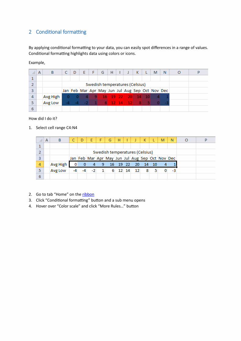
2 Conditional formatting

By applying conditional formatting to your data, you can easily spot differences in a range of values.

Conditional formatting highlights data using colors or icons.

Example,

How did I do it?

1. Select cell range C4:N4

2. Go to tab “Home” on the ribbon

3. Click “Conditional formatting” button and a sub menu opens

4. Hover over “Color scale” and click “More Rules…” button

5. Click Minimum color and pick a blue color.

6. Click Maximum color and pick a red color.

7. Click OK

Repeat above steps with cell range C5:N5.

2.1 Conditional formatting – formula You can use a formula to determine which cells to format. Now conditional formatting becomes really

powerful!

Example, here is a list. Are there any duplicates? Not that easy to identify, but wait!

1. Select the data

2. Go to tab “Home” on the ribbon

3. Click conditional formatting button

4. Click “New Rule..”

5. Click “Use a formula to determine which cells to format”, see pic above.

6. Type: =COUNTIFS($A$2:$A$12,$A2,$B$2:$B$12,$B2,$C$2:$C$12,$C2)>1

in “Format values where this is true:”

7. Click “Format…” button

8. Click “Fill” tab

9. Pick a color.

10. Click OK

11. Click OK

Duplicate records are now highlighted! Read more:

Highlight duplicates where adjacent cell value meets criteria using conditional formatting

3 Sort & Filter Working with data is really easy in excel. The following example demonstrates how to quickly sort or

filter data.

1. Select a cell in the data

2. Press CTRL + SHIFT + L

3. Click the arrow in the column header to choose a filter for the column

4. Here you can choose to sort values or only show all records containing Alba. If you have large

data sets, use the search field!

4 Data Validation

4.1 Data Validation What is data validation? You can control what is being entered in a worksheet. If a user enters data

that is not allowed, a warning message appears.

You can create drop down lists or data validation lists (they are the same), you can restrict entries or

create your own rules.

Example – drop down lists

1. Select cell B3

2. Go to tab “Data” on the ribbon

3. Click “Data validation” button

4. Go to tab “Settings”

5. Select List (see pic above)

6. Type: =$E$3:$E$8 in source field

7. Click OK

You have now created a drop down list in cell B3.

4.2 Data Validation – Prevent duplicate records In this example I am trying to prevent the user from entering a duplicate record.

1. Select cell range B3:D20

2. Go to tab “Data”

3. Click “Data validation” button

4. Select Custom

5. Type formula: =COUNTIFS($B$3:$B$20,$B3,$C$3:$C$20,$C3,$D$3:$D$20,$D3)<=1

6. Click OK

See picture below.

Let´s see what happens if I type a duplicate record.

5 Excel defined tables

5.1 Quickly create an Excel defined table

1. Select a data set

2. Press CTRL + T

So why use tables?

Use table names in formulas

Dynamic (add values and they expand automatically)

Formulas in a table cell are entered in the entire column immediately

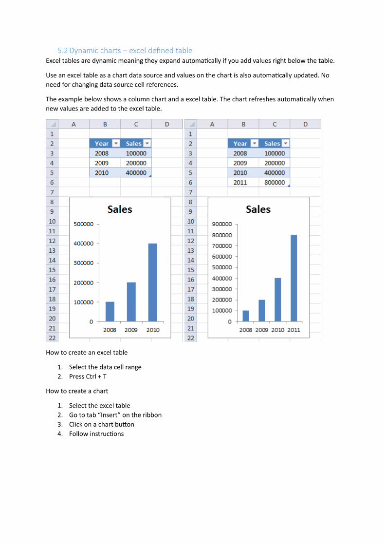
5.2 Dynamic charts – excel defined table Excel tables are dynamic meaning they expand automatically if you add values right below the table.

Use an excel table as a chart data source and values on the chart is also automatically updated. No

need for changing data source cell references.

The example below shows a column chart and a excel table. The chart refreshes automatically when

new values are added to the excel table.

How to create an excel table

1. Select the data cell range

2. Press Ctrl + T

How to create a chart

1. Select the excel table

2. Go to tab “Insert” on the ribbon

3. Click on a chart button

4. Follow instructions

6 Excel named ranges

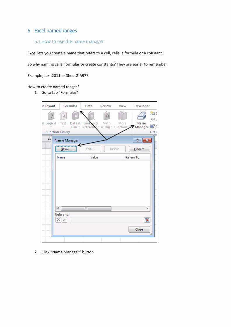
6.1 How to use the name manager

Excel lets you create a name that refers to a cell, cells, a formula or a constant.

So why naming cells, formulas or create constants? They are easier to remember.

Example, taxn2011 or Sheet2!A97?

How to create named ranges?

1. Go to tab “Formulas”

2. Click “Name Manager” button

3. Click “New” button

4. Enter a name

5. In the “Refers to:” you can:

a. Select a cell or a

b. cell range or

c. type a formula

d. Type a constant

6. Click OK

How to use a named range

1. Start typing the named range and it shows up in the cell or the formula bar

2. Select or click on the name

6.2 Quickly open the name manager (keyboard shortcut)

Press CTRL + F3

6.3 Show named ranges

Working with many named ranges can be confusing. How do you quickly find the right one?

1. Select a cell

2. Press F4

3. The “Paste Name” dialog box shows up.

4. Select a name

5. Click OK

6.4 Quickly create a named range

1. Select a cell or cell range

2. Click in name box

3. Type a name

4. Press Enter

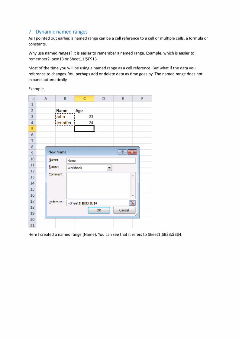
7 Dynamic named ranges As I pointed out earlier, a named range can be a cell reference to a cell or multiple cells, a formula or

constants.

Why use named ranges? It is easier to remember a named range. Example, which is easier to

remember? taxn13 or Sheet11!$F$13

Most of the time you will be using a named range as a cell reference. But what if the data you

reference to changes. You perhaps add or delete data as time goes by. The named range does not

expand automatically.

Example,

Here I created a named range (Name). You can see that it refers to Sheet1!$B$3:$B$4.

Here I changed the cell reference to a formula. Now the named range automatically expands when

you add or remove data.

Formula:

=Sheet1!$B$3:INDEX(Sheet1!$B:$B,COUNTA(Sheet1!$B:$B)+1)

Why use dynamic named ranges when you can use excel tables? It is a matter of personal preference.

I think it is easier to setup (select data and press Ctrl + T) and use excel tables.

But using table names is not always so easy, for example you need a workaround to use excel table

names in conditional formatting or data validation (See excel tables). Also, if you are not used to how

to reference table names in formulas, they can sometimes be confusing.

8 Visual basic for applications

8.1 Enable Developer tab on the ribbon

The Developer tab on the ribbon lets you work with macros.

Excel 2007

1. Click the Microsoft Office Button 2. Click Excel Options 3. Click Popular, and then 4. Select the Show Developer tab in the Ribbon check box.

Excel 2010

1. Click File tab on the ribbon

2. Click Options

3. Click Customize ribbon

4. Select Developer, see pic to the right

5. Click OK

8.2 Macro recorder – learn vba The macro recorder lets you record commands you perform. You can then easily examine the code

and quickly learn new vba functions.

Example,

How do I change the column width for all columns in a sheet?

1. Go to tab “Developer”

2. Click “Record macro” button

3. Select all cells

4. Change column width for a column, click and hold on a column line.

5. Drag to right or left to change column width

6. Go to tab “Developer”

7. Click “Stop recording” button

8. Click “Visual basic” button or press Alt + F11

9. Examine the code

8.3 Quickly open VB Editor using a keyboard shortcut Press Alt + F11 and WB Editor opens.

You create subroutines (macros) and custom functions or user defined functions in a module.

8.4 Assign a macro to a button

1. Go to Developer tab on the ribbon

2. Click “Insert” button

3. Click “Button” (Form Control), see picture above

4. Draw a button on the sheet

5. Select a macro

6. Click OK

You can also

1. Right click on a button on a sheet

2. Click “Assign macro”

3. Select a macro

4. Click OK

9 Keyboard shortcuts

9.1 Press Alt key to see available keyboard short cuts Example, here is a picture of the ribbon.

Here is what happens if you press Alt key.

Press N and you will go to the “Insert” tab on the ribbon.

Each button on the tab “Insert” is assigned a character. For example, press V to build a pivot table.

You can also hover over a button on the ribbon and in most cases the keyboard shortcut is shown.

Hovering over Table button displays this window and it tells you that you can press CTRL + T to create

a table.

9.2 Shortcut keys to quickly enter todays date in a cell

1. Select a cell

2. Press and hold CTRL + SHIFT

3. Press ; once

4. Release all keys

9.3 Short cut keys to enter current time in a cell 1. Select a cell

2. Press and hold CTRL + SHIFT

3. Press ; once

4. Release all keys

9.4 Keyboard Short cut -Jump to next empty cell The following picture shows a data set. You want to know if there are any blank cells in column A.

1. Select cell A2

2. Press Ctrl + arrow down key

You are instantly taken to the cell above the next empty cell. If there are no empty cells you will be

taken to the last cell in the data set.

There is a blank cell in this example.

9.5 Quickly select a data range You can quickly select cell range B2:D12 by selecting a cell in the data set.

Then press CTRL + A.

9.6 Select the entire column or row

Select entire column

You have two options:

1. Click on column name

2. or select a cell in column you want to select and then press CTRL + Space

Select entire row

You have two options:

1. Click on row number

2. or select a cell in row you want to select and then press Shift + Space

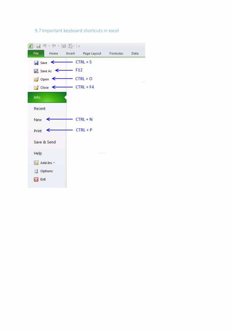
9.7 Important keyboard shortcuts in excel

10 Quickly format a cell

Ctrl + ! Ctrl + Shift + 1 General formatting with two decimals Ctrl + @ Ctrl + Shift + 2 Format for time Ctrl + # Ctrl + Shift + 3 Apply date formatting Ctrl + $ Ctrl + Shift + 4 Currency format Ctrl + % Ctrl + Shift + 5 Apply percentage formatting Ctrl + ^ Ctrl + Shift + 6 Scientific formatting Ctrl + & Ctrl + Shift + 7 Applies a single border Ctrl + * Ctrl + Shift + 8 Select a contiguous range of cells

11 Excel formulas

11.1 Evaluate formula “Evaluate formula” dialog allows you to debug a formula by evaluating each part of the formula

individually.

1. Go to tab “Formulas” on the ribbon

2. Click “Evaluate Formula” button

3. Click “Evaluate” button to see each part of the formula individually. (See pic below)

The formula in cell B2 returns an error. The “Evaluate formula” dialog allows you to examine the

formula to see why it returns an error.

11.2 Change relative cell ref to absolute cell ref Entering cell references in a formula is a common task but did you know that you can easily convert

the relative cell reference by pressing F4?

Example,

Here is a relative cell reference. (picture above) Now press F4.

The cell reference changes to a absolute cell reference. Press F4 again.

This time only the row reference is locked. Press F4 again.

The column reference is locked. Press F4 again and the cell reference becomes relative again.

Want to know more about relative and absolute cell references? Check out my blog post:

Absolute and relative references in excel

11.3 Convert cell reference to values You can convert a cell reference to constants in a formula.

1. I created a simple formula, a cell reference to B3:B6

2. Select the cell reference in the formula bar

3. Press F9

11.4 Enter a value or a formula in empty cells The picture below shows some names in cell range B3:B12, there are also blank cells. Let´s fill those

blank cells with a character.

1. Select cell range B3:B12

2. Press F5

3. Click “Special…” button

4. Click “Blanks”

5. Click OK

6. Click in formula bar (see pic above)

7. Type –

8. Press CTRL + ENTER

All blank cells contain character -.

This example has only a small cell range, imagine if you work with a much larger cell range. A real

time saver!

You can also enter a formula or an array formula in those blank cells!

11.5 Use INDEX + MATCH instead of VLOOKUP

Formula in cell C10:

=VLOOKUP(B10,B3:D6,2,FALSE)

The VLOOKUP function looks for a matching value in the leftmost column. Example, if you want to

look for an Item and return the corresponding year, VLOOKUP can´t do it! But the INDEX and MATCH

function can.

INDEX + MATCH

Formula in cell C10:

=INDEX($B$3:$B$6,MATCH(B10,$C$3:$C$6,0))

The MATCH function returns the relative position of an item in a cell range. MATCH(B10,$C$3:$C$6,0)

returns 1.

INDEX($B$3:$B$6,MATCH(B10,$C$3:$C$6,0)) becomes INDEX($B$3:$B$6,1) and returns 2011.

11.6 Concatenate cell values The CONCATENATE function lets you concatenate values but with on big disadvantage. You can´t use a

cell range as an argument. You have to enter each cell reference, see picture below.

Here is a workaround:

1. Type: =CONCATENATE( in the formula bar

2. Select a cell range

3. Select the cell range in the formula bar

4. Press F9

5. Remove the curly brackets { }

6. Replace ; with a ,

7. Type ) at the end of the function

8. Press Enter

11.7 Autosum

Excel can sum values for you, here is how to do it:

1. Select cell B10

2. Go to tab “Home” on the ribbon

3. Click Autosum button or press Alt + =

4. Press Enter

11.8 Copy formula and paste value If you want to copy the value and paste it to another cell, copy paste won´t work if you have a

formula in the cell.

Here is how to copy the value only:

1. Select the cell

2. Copy cell or press CTRL + C

3. Right click on the destination cell

4. Hover over “Paste Special…”

5. Click on “Paste Values” button, see picture below

12 Transpose values in a column to a row The two pictures below demonstrate values being transposed from a column to a row.

Instructions

1. Select cell range B2:B5

2. Copy (Ctrl + c)

3. Right click on cell C2

4. Click “Paste special…”

5. Select “Transpose”, see picture above.

6. Click OK

13 Transpose a table The two pictures below demonstrate a data set being transposed.

Instructions

1. Select cell range B2:C6

2. Copy (Ctrl + c)

3. Right click on cell D2

4. Click “Paste special…”

5. Select “Transpose”, see picture above.

6. Click OK

14 Formatting

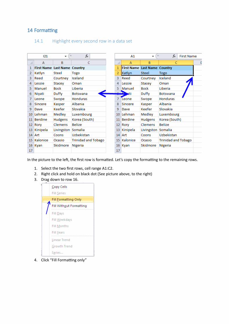
14.1 Highlight every second row in a data set

In the picture to the left, the first row is formatted. Let’s copy the formatting to the remaining rows.

1. Select the two first rows, cell range A1:C2.

2. Right click and hold on black dot (See picture above, to the right)

3. Drag down to row 16.

4. Click “Fill Formatting only”

14.2 Hide values in a sheet

The following formula in cell D3 counts how many non empty values there are in cell range B3:B20.

But you don´t want to show the cell and the calculation to the user.

How to hide the value

1. Select cell D3

2. Press CTRL + 1

3. Select Custom

4. Type ;;;

5. Click OK

The value is hidden but still there!

14.3 Quickly format a cell or a cell range

1. Select cell

2. Press CTRL + 1

3. Format the cell as you desire

4. Click OK

14.4 Double click format painter to copy and paste formats to other cells

The format painter allows you to copy formatting from one place and apply it to another.

Double click to apply the same formatting to multiple places in the document.

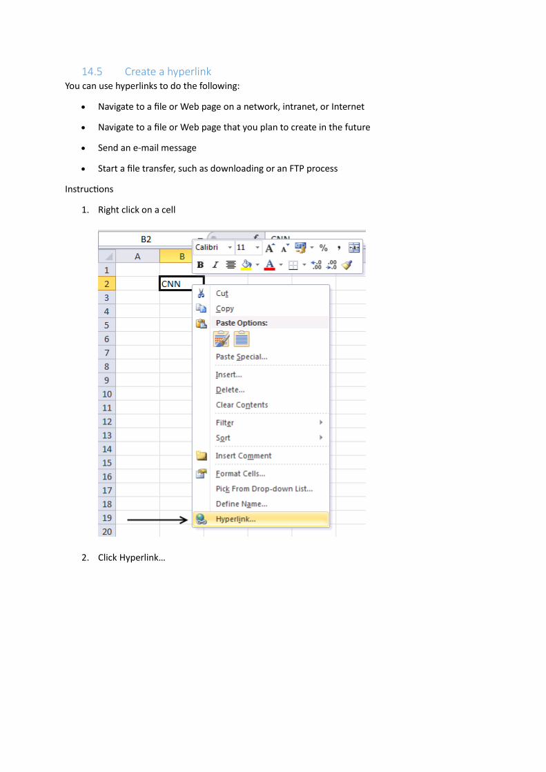
14.5 Create a hyperlink You can use hyperlinks to do the following:

Navigate to a file or Web page on a network, intranet, or Internet

Navigate to a file or Web page that you plan to create in the future

Send an e-mail message

Start a file transfer, such as downloading or an FTP process

Instructions

1. Right click on a cell

2. Click Hyperlink…

3. Enter address

4. Press OK

TIP! Keyboard short cut: Ctrl + K

Read more: Create, select, edit, or delete a hyperlink

15 Working with cells

15.1 Edit a cell

You have two options if you want to edit a cell.

Double click the cell

Press F2

Pressing F2 places the insertion point after the active cell’s content.

On the other hand, double clicking on a cell allows you to choose where the insertion point is being

placed.

15.2 How to quickly change multiple column or row widths on a sheet

1. Select the columns (Use Ctrl + mouse to select multiple non adjacent columns)

2. Click and drag the column border to the right or left

3. Release mouse button

Tip! Click this button to select all rows and columns.

15.3 Quickly hide and unhide a column or a row using a keyboard shortcut How to hide row

1. Select a row (or many)

2. Press CTRL + 9

How to unhide a row

1. Select rows surrounding the hidden rows

2. Press CTRL + SHIFT + 9

15.4 Undo, redo or repeat command (keyboard shortcuts)

Undo command

Keyboard shortcut: Press CTRL + z

Redo command

Keyboard shortcut: Press CTRL + y

Repeat command

Keyboard shortcut: Press function key F4

15.5 Quickly select all cells with comments

The following picture shows three cells with comments:

You can quickly select these cells by pressing CTL + Shift + o (not zero)

This is really useful if you want to delete all comments in sheet:

1. Right click on a selected cell

2. Click “Delete comment”

15.6 Copy | Paste | Cut

Copy

1. Select a cell or cell range

2. Click Copy button

3. or press CTRL + C

Cut

1. Select a cell or cell range

2. Click Cut button

3. Or press CTRL + X

Paste

1. Select a destination cell

2. Click Paste button or press CTRL + V

15.7 Enter a new row in a cell

If you have a lot of data in one cell, it can be helpful to use new rows inside the cell.

Here is how to do it:

1. Select a cell

2. Type whatever you want to type

3. Press Alt + Enter to enter a new row in the cell

4. Repeat step 2 and 3

5. Lastly, press Enter

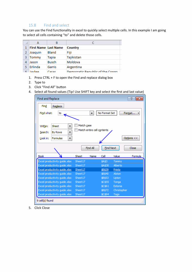
15.8 Find and select You can use the Find functionality in excel to quickly select multiple cells. In this example I am going

to select all cells containing “to” and delete those cells.

1. Press CTRL + F to open the Find and replace dialog box

2. Type to

3. Click “Find All” button

4. Select all found values (Tip! Use SHIFT key and select the first and last value)

5. Click Close

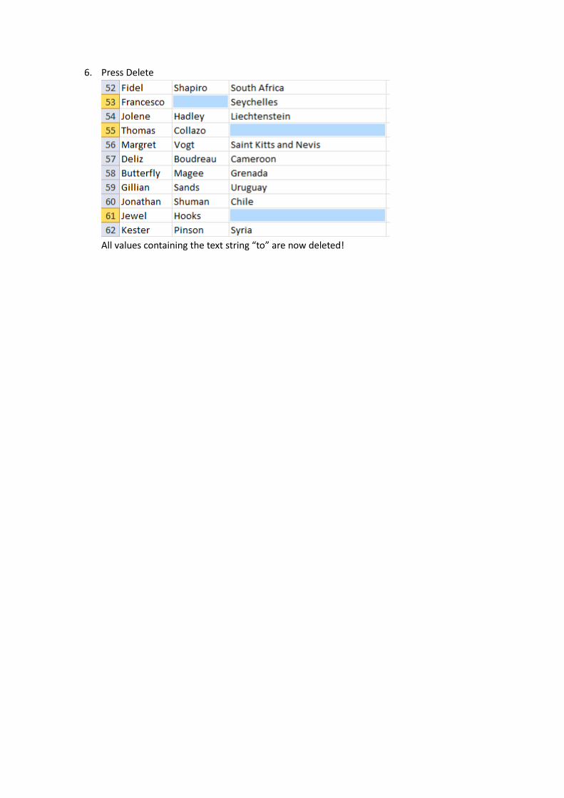
6. Press Delete

All values containing the text string “to” are now deleted!

16 Working with excel sheets

16.1 Shortcuts for managing sheets Shortcut key Shift + F11 allows you to insert a new sheet. You can also click this button:

Navigating between sheets

Keyboard short cut CTRL + Page Up navigates to the previous sheet in the list at the bottom of the

screen.

Keyboard short cut CTRL + Page Down navigates to the next sheet in the list at the bottom of the

screen.

16.2 Double click a sheet name to rename it You can quickly rename a sheet by double clicking the sheet name at the bottom of the screen.

Type the new name

or click on sheet name to choose the insertion point.

16.3 Multiple views of the same worksheet

This tip is great if you want to see different parts of the same sheet (or workbook) at the same time.

Go to tab ”View” on the ribbon

Click “New window”

Click “View Side by Side”

Click “Arrange all”

Click “Horizontal” or “Vertical” and then press OK.

17 Excel charts

17.1 Months and years in a chart This technique allows you to group chart categories like months into years.

Look at this chart.

The dates on the x-axis are hard to read. Now, add a new column “Year” and change the x-axis values

in the chart so they include the new column. Make sure the months are sorted and that only the first

record contains the year. This is what you get:

Here you can see that the year column only contains a single unique year value. If you have multiple

year values you will get duplicates in the chart.

It is a lot more readable now and nicer!

Instructions

1. Right click on chart

2. Click “Select Data…”

3. Adjust the chart data range

4. Click OK!

18 Ribbon

18.1 Show / Hide the ribbon

Double click a tab on the ribbon or press CTRL + F1

The ribbon is collapsed. Double click again or press CTRL + F1 to show the ribbon.