Excel Intermediate Training Packet - Shasta County … LEFT, MID, and RIGHT Formula Syntax English...
32
Excel Intermediate Table of Contents Formulas UPPER, LOWER, PROPER AND TRM.....................................................................................................2 LEFT, MID, and RIGHT..........................................................................................................................3 CONCATENATE ....................................................................................................................................4 & (Ampersand) ....................................................................................................................................5 CONCATENATE vs. & (Ampersand) ......................................................................................................5 ROUNDUP, and ROUNDDOWN ...........................................................................................................6 VLOOKUP .............................................................................................................................................7 HLOOKUP.............................................................................................................................................9 IF ..........................................................................................................................................................10 Nested IF .............................................................................................................................................11 IF and AND..........................................................................................................................................12 SUMIF ..................................................................................................................................................13 Error Values in Excel ............................................................................................................................14 Charts Ribbon Tour .........................................................................................................................................14 Creating a chart ...................................................................................................................................15 Chart Layout Options...........................................................................................................................16 Multiple Series within a chart .............................................................................................................17 Modifying Gridlines .............................................................................................................................21 Filters Ribbon Tour .........................................................................................................................................23 Quick Filtering .....................................................................................................................................23 Filtering by multiple criteria ................................................................................................................25 Saving Filtered Data.............................................................................................................................27 Text to Columns (Data Parsing) UPPER, LOWER, PROPER AND TRIM....................................................................................................28
Transcript of Excel Intermediate Training Packet - Shasta County … LEFT, MID, and RIGHT Formula Syntax English...

Excel Intermediate
Table of Contents
Formulas
UPPER, LOWER, PROPER AND TRM .....................................................................................................2
LEFT, MID, and RIGHT ..........................................................................................................................3
CONCATENATE ....................................................................................................................................4
& (Ampersand) ....................................................................................................................................5
CONCATENATE vs. & (Ampersand) ......................................................................................................5
ROUNDUP, and ROUNDDOWN ...........................................................................................................6
VLOOKUP .............................................................................................................................................7
HLOOKUP .............................................................................................................................................9
IF ..........................................................................................................................................................10
Nested IF .............................................................................................................................................11
IF and AND ..........................................................................................................................................12
SUMIF ..................................................................................................................................................13
Error Values in Excel ............................................................................................................................14
Charts
Ribbon Tour .........................................................................................................................................14
Creating a chart ...................................................................................................................................15
Chart Layout Options...........................................................................................................................16
Multiple Series within a chart .............................................................................................................17
Modifying Gridlines .............................................................................................................................21
Filters
Ribbon Tour .........................................................................................................................................23
Quick Filtering .....................................................................................................................................23
Filtering by multiple criteria ................................................................................................................25
Saving Filtered Data.............................................................................................................................27
Text to Columns (Data Parsing)
UPPER, LOWER, PROPER AND TRIM ....................................................................................................28

2
Formulas
UPPER, LOWER, PROPER, and TRIM
These formulas all work with text. After using one of these functions it is good practice to paste special\values so
that they will remain in their desired formatting.
UPPER, LOWER, PROPER, and TRIM
Formula Description
=UPPER Converts all text to upper case
=LOWER Converts all text to lower case
=PROPER Capitalizes the first letter in a text string and any other letters in text that follow any character other than a letter, i.e. a space. Converts all other letters to lowercase
=TRIM Removes all blank, unnecessary spaces at the start and end of a string including extra spaces, tabs, and other characters that don’t print.
LEFT, MID, and RIGHT
When data is imported or copied into an Excel spreadsheet unwanted characters or words can sometimes be
included with the new data. Excel has several functions that can be used to remove such unwanted characters.
Which function you use depends upon where the unwanted characters are located:
If the unwanted characters are on the right side of your good data, use the LEFT function to remove them.
If you have unwanted characters on both sides of your good data, use the MID function to remove them.
If these unwanted characters appear on the left side of your good data, use the RIGHT function to remove them.
1 2 3

3
LEFT, MID, and RIGHT
Formula Syntax English Translation =LEFT =LEFT(text, num_chars) Using the piece of data you want, typically a cell
reference, indicate how many characters you want used/ brought back starting at the left most position.
=MID =MID(text, start_num,num_chars) Using the piece of data you want, typically a cell reference, indicate the first character to be used starting at the left most position and how many characters to the right of the start number to be used/brought back.
=RIGHT =RIGHT(text, num_chars) Using the piece of data you want, typically a cell reference, indicate how many characters you want used/ brought back starting at the rightmost position. .
To increase the power of LEFT formula combine it with a FIND. Instead of counting the number of spaces you have
to move through the cell, key of a constant. Below is a screen shot of a listing of name, location, and gender. The
location includes both the city and state. The desire is to separate the city and state into two fields.
In order to separate the city utilizing the LEFT command, there are a couple of options.
1. The common one of specifiying the number of characters that it needs to move over. This is difficult due
to them being of different lengths.
2. Or instruct the formula to bring back the characters after the FIND command locates what it is looking for.

4
Utilizing the common LEFT will not work in this scenario because the length of the city names is not consistent.
Redding in D1 is just fine; however Palo Cedro is cut off because it is longer.
By combining the FIND with the LEFT, you can quickly get exactly what you want. The negative one (1) is added
because if not, the comma would be returned as well.
CONCATENATE
The CONCATENATE function is used to join two or more words or text strings together. After using this function it
is good practice to paste special\values so that they will remain in their desired formatting.
The syntax is =CONCATENATE(A1,B1,C1….)
The finished product is quite literally a combination of the text without any spaces. If spaces are desired, there are
two options. The first to add within your formula the cell reference where there is a space as the only value within
the cell value, or to add a space within the formula. Since text is being added, it must be lead and followed by a
double quote (“). An example is =CONCATENATE(A1,” “,B1,” “,C1).
An example of CONCATENATE is below and combined with & due to their interchangeability.
2
1

5
& (Ampersand)
The & connects, or concatenates, multiple values to produce one continuous text value. After using this function it
is good practice to paste special\values so that they will remain in their desired formatting.
CONCATENATE vs. & (Ampersand)
Besides CONCATENATE sounding smarter, and worth fifteen points in Scrabble, the two functions are
interchangeable and really come down to personal preference. CONCATENATE formulas tend to be a bit easier to
read.
Either function may be used to combine words or phrases that are not part of the range. For instance, we want to
fill in the blanks for the following sentence:
Famous February birthdays are ______ and ______.
And we have the following data table:

6
By utilizing the CONCATENATE formula, we can substitute text located in cells within our spreadsheet into a
completed sentence.
ROUNDUP and ROUNDDOWN
The ROUNDUP function is used to round a number upwards toward the next highest number. Although similar to
ROUND, ROUNDUP always rounds upward whereas ROUND will round up or down depending on whether the last
digit is greater than or less than five (5).
Although the ROUNDUP can be a standalone formula, it is often nested with other formulas, for example SUM. It is
especially useful with division due to the fractions that are often created.

7
VLOOKUP
The VLOOKUP function searches vertically (top to bottom) the leftmost column of a table until a value that matches or exceeds the one you are looking up is found.
The elements being looked up must be unique and must be arranged or sorted in ascending order; that is, alphabetical order for text entries, and lowest‐to‐highest order for numeric entries.
The syntax is =VLOOKUP(lookup_value,table_array,col_index_num,[range_lookup]).
An example of the formula is: VLOOKUP(E2,D2:M3,2,TRUE) The English translation is using the value found in the cell E2, look in the range of D2 to M3 row by row. If you find a value that matches or exceeds the value in E2, using that row, go over 2 columns to the right, grab the value there and bring it back.
There are two range_lookup argument options; TRUE or FALSE
TRUE
Is the default answer, so you may leave it out of the formula
Looks for an approximate match
If it finds an exact match it will use it.
If it doesn’t find an exact match, it will use the last item before it got greater
Alphabetical: Looking for Cat. If elements are Apple, Bird, Carpet, Dog; then Carpet
would be returned because Dog exceeds Cat alphabetically.
Numeric: Looking for 5.25. If elements are 3.0, 4.0, 5.0, 6.0, 7.0, then 5.0 would be used.
The last number before 5.25 was exceeded.
FALSE
Looks for an exact match.
If it finds an exact match it will use it.
If it doesn’t find an exact match, it will return #N/A
Alphabetical: Looking for Cat. If elements are Apple, Bird, Carpet, Dog; then #N/A would
be returned.
Numeric: Looking for 5.25. If elements are 3.0, 4.0, 5.0, 6.0, 7.0, then #N/A would be
returned because there is no exact match.

8

9
HLOOKUP
The HLOOKUP function searches horizontally (left to right) the topmost column of a table until a value that matches or exceeds the one you are looking up is found.
The elements being looked up must be unique and must be arranged or sorted in ascending order; that is, alphabetical order for text entries, and lowest‐to‐highest order for numeric entries.
The syntax is =HLOOKUP(lookup_value,table_array,row_index_num,[range_lookup])
An example of the formula is: HLOOKUP(E2,D2:M3,2,TRUE) The English translation is using the value found in the cell E2, look in the range of D2 to M3 and go column by column. If you find a value that matches or exceeds the value in E2, using that row, go down 2 rows to the right, grab the value there and bring it back.
There are two range_lookup argument options; TRUE or FALSE
TRUE
Is the default answer, so you may leave it out of the formula
Looks for an approximate match
If it finds an exact match it will use it.
If it doesn’t find an exact match, it will use the last item before it got greater
Alphabetical: Looking for Cat. If elements are Apple, Bird, Carpet, Dog; then Carpet
would be returned because Dog exceeds Cat alphabetically.
Numeric: Looking for 5.25. If elements are 3.0, 4.0, 5.0, 6.0, 7.0, then 5.0 would be used.
The last number before 5.25 was exceeded.
FALSE
Looks for an exact match.
If it finds an exact match it will use it.
If it doesn’t find an exact match, it will return #N/A
Alphabetical: Looking for Cat. If elements are Apple, Bird, Carpet, Dog; then #N/A would
be returned.
Numeric: Looking for 5.25. If elements are 3.0, 4.0, 5.0, 6.0, 7.0, then #N/A would be
returned because there is no exact match.

10
IF
The formula makes a statement/question, if the answer is true then one response is obtained. If the answer if
false, then another answer is obtained.
The syntax is =IF(logical_test,value_if_true,value_if_false)
The formula is =IF(G6>0, ”Have money left to spend.”,”Houston, we have a problem”). The English translation is if
the value found in G6 is greater than zero THEN display the comment ‘Have money left to spend.ELSE display the
comment ‘Houston, we have a problem’.
Nested IF
A nested IF command is merely multiple if statements within the same formula.
The formula is =IF(G8>0, ”Have money left to spend.”,IF(G8<‐5000,”We are in it deep!”,”Houston, we have a
problem”). The English translation is if the value found in G8 is greater than zero THEN display the comment ‘Have
money left to spend.’ IF it is less than Negative 5,000 then display ‘We are in deep!’ ELSE display the comment
‘Houston, we have a problem’.
IF & AND
The AND function is a logical function which generates an output of either TRUE or FALSE. By itself, the AND
function has limited usefulness. However, combining it with other functions, such as the IF, greatly increases the
capabilities of a spreadsheet.

11
The syntax is of the IF is: =IF(logical_test,value_if_true,value_if_false) and the syntax of the AND is: =AND(logical1,
logical2, …) with only one logical being required. With that being said the combined syntax is simply the AND
replacing the logical_test parameter: =if(AND(logical1, logical2,…,value_if_true,value_if_false).
The formula is =IF(AND(D10<C10,G10<0),”We made a bad budget adjustment”,”Budget adjustment was a good
one’). The English translation is IF the revised budget is less than the Adopted budget AND account balance is less
than zero THEN display ‘We made a bad budget adjustment’ ELSE display ‘Budget adjustment was a good one.’
SUMIF
What about those times when you only want the total of certain items within a cell range? For those situations,
you can use the SUMIF function. The SUMIF function enables you to tell Excel to add together the numbers in a
particular range only when those numbers meet the criteria that you specify. The syntax of the SUMIF function is
as follows:
=SUMIF(range,criteria,[sum_range])
In the SUMIF function, the range argument specifies the range of cells that you want Excel to evaluate when doing
the summing; the criteria argument specifies the criteria to be used in evaluating whether to include certain values
in the range in the summing; and finally, the optional sum_range argument is the range of all the cells to be
summed together. If you omit the sum_range argument, Excel sums only the cells specified in the range argument
(and, of course, only if they meet the criteria specified in the criteria argument).
Below is an excert from our mileage report. Totals by employee are desired. There are a variety of ways to
accomplish it. SUMIF is a great solution for this very task.
The formula is =SUMIF(A2:E18,A21:A26,E2:E18). The English translation is look within the range of A2 and E18, and
look for the information found in A21:A26, when you locate a match, add up the values found within E2 and E18.

12
13
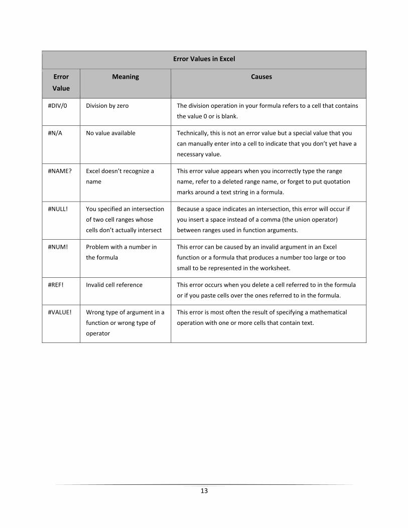
Error Values in Excel
Error
Value
Meaning Causes
#DIV/0 Division by zero The division operation in your formula refers to a cell that contains
the value 0 or is blank.
#N/A No value available Technically, this is not an error value but a special value that you
can manually enter into a cell to indicate that you don’t yet have a
necessary value.
#NAME? Excel doesn’t recognize a
name
This error value appears when you incorrectly type the range
name, refer to a deleted range name, or forget to put quotation
marks around a text string in a formula.
#NULL! You specified an intersection
of two cell ranges whose
cells don’t actually intersect
Because a space indicates an intersection, this error will occur if
you insert a space instead of a comma (the union operator)
between ranges used in function arguments.
#NUM! Problem with a number in
the formula
This error can be caused by an invalid argument in an Excel
function or a formula that produces a number too large or too
small to be represented in the worksheet.
#REF! Invalid cell reference This error occurs when you delete a cell referred to in the formula
or if you paste cells over the ones referred to in the formula.
#VALUE! Wrong type of argument in a
function or wrong type of
operator
This error is most often the result of specifying a mathematical
operation with one or more cells that contain text.

14
Charts
Ribbon Tour
Chart icons are found on the Insert ribbon tab. Not all tabs are constant on the ribbon; many appear
only once you have selected that particular item. Charts are an example. Once you have a chart in your
workbook and select the below tab appears as below, typically to the far right of the standard tabs.
The Chart Tools tabs are Design, Layout, and Format
Chart Tools Design Tab
1 Change Chart Type: using the current chart data, allows you to choose another type: columns, line, pie, bar, area, etc.
2 Switch row/column: alternates between the values displayed on the horizontal axis and the series
3 Quick Layout: allows you to chose from various pre‐formatted charts
4 Choose amongst a multitude of color schemes
1 2 3 4

15
Chart Tools Layout Tab
1 Drop down box depicting a variety of chart components that can then be formatted or edited independently
2 Quick drop down for Chart Title options
3 Quick drop down for Axis Titles options
4 Quick drop down for Legend options
Chart Tools Format Tab
1 Drop down box depicting a variety of chart components that can then be formatted or edited independently
2 Quick drop down for shape fills
3 Quick drop down for shape outlines
2
1
3
4
1 2
3

16
Creating a Chart
There are a multiple ways to create and modify a chart. The below are a few straight forward steps that highlight
options of completing your chart.
Step Creating a Basic Chart
1 Highlight the area you would like to make a chart for.
2 Create a chart by using an icon for the type of chart desired, i.e. column, line, etc
3 Chose colors for your chart, if the default is not what is desired
4 Select chart layouts. Specifically title, vertical & horizontal labels, and legends
Chart Layout Options
Chart Layouts
Layout Title Vertical (Y)
Labels
Horizontal (X)
LabelsLegend Series Labels
1 Top, Centered Left Below Right
2 Top, Centered Within chart Below Top
3 Top, Centered Left Below Below
4 None Left Below Below Within chart
5 Top, Centered Left Below Below Below

17
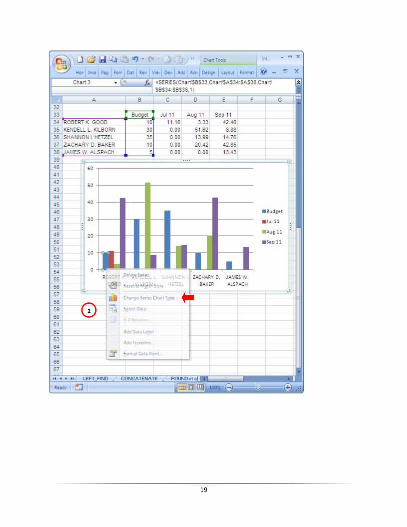
Multiple series within chart types
You may have multiple series types on a single chart. For example, you may want bars as well as a single line representing different data. To do so, create chart as usual. Then perform the following steps:
Step Description
Select the series you want to be different. Notice that small circles appear at all corners of
the series you selected
Right click you mouse and select Change Series Chart Type
Change chart type dialog box will appear, select the type you desire
Layout 4
1
2
3

18
1
19
2

20
3

21
Modifying Grid Lines
Excel will come up with its best guess as to what the gridlines should be. You may find the need to adjust these to
something more to your liking.
Hover anywhere over the vertical axis and left click your mouse.
Notice:
The numbers are now outlined by a box
Once you are on the Chart Tools Layout
Tab, the current selection box is presented.
The Vertical (Value) axis appears in the
current selection group.
By left clicking on the Format Selection
1
2
3 1
2
3
4
4

22
The Format Axis dialog box will appear. By
selecting the fixed radio button on any option,
you may manipulate any value that you would
like.

23
Filters
Ribbon Tour
Quick Filtering
The secret to filtering is not to have a space between your titles and your data. In fact, Excel is so smart, that you
do not even have your data selected, but may if you prefer.
Select your data and left click on the
filter icon in the Sort & Filter Group.
Notice that a chevron appears to the
left of each header.

24
By selecting the chevron to the left of Vendor Name, a dialog box
appears displaying all unique text filters found in the range as
well as other common sort icons.
If you only want a particular filter, deselect the (Select All) box
and check the filter you desire.
In the below screen shot, Kendell Kilborn is selected. Notice the hidden rows to the left. Those represent
data lines for mileage paid to individuals other than Kendell. No data is lost, it is just currently hidden.
Also note that the icon to the left of
the vendor name now displays the filter icon.
This so at a glance the user may see that the
data range has been filtered.

25
Filtering by Multiple Criteria
The filtering tool is fine when you only want one item. However the power of the advance filter tool really shines
when you want to sort by multiple criteria. There are several thou shalts of advanced filtering.
Thou Shalts of Advanced Filtering
1 The headers in the criteria range must be exactly as they are in the list range
2 There must be at least one blank row between the criteria range and the list range
Steps For Advanced Filtering
Create a criteria range by inserting a few rows and copying the header from the data range.
Although not required, it is often best to have the range above your data for simplicity.
Type in the criteria you want to filter by.
Have your curser somewhere in the data range
Select the Advanced icon with your left mouse button.
The list range most likely will be your data. If not, you will need to correct it.
Select your criteria range.
The range must include the headers of the criteria range
The rows with criteria
All columns in the range
Select OK
:
6
1
2
3
4
5
7

26
1 2
4
5

27
The results appear below.
Saving the Filtered Data
Now that the data has been filtered it would be great to save it so you can manipulate it further. To do so is a
rather straight forward process. Basically you will go to where you want to save it, Sheet2 in our example, and go
through the filtering process that we did above with just a couple of twists.
Steps For Advanced Filtering
On the destination worksheet (Sheet2 for example) place the cursor in a blank cell.
Select the Advanced icon with your left mouse button.
Under Action, select copy to another location
1
2
3

28
In the list range, select the range finder icon.
The appears. Navigate to the appropriate
worksheet and select the data range not forgeting the headers, and click on the
little icon at the bottom right.
Do the same for the criteria range.
For the copy to range, select the first cell and select OK
Text to Columns
Text to columns, previously known as data parsing, is a powerful data manipulation tool. Similar to LEFT, MID, and
RIGHT, it is used to split combined data into separate columns, such as first and last names; or city, state, and zip
codes. It is also handy when exports from Escape brings over a number value as a text field.
Using Text to Columns
1 If necessary, insert blank columns to the right of the cells you want to convert into multiple columns.
NOTE: Excel will use the original column as the first column to write over. If you will need a total of three columns, for instance separating city, state, and zip, you will need to add two columns.
NOTE: You may override Excel’s desire to write over the first column by changing the column letter.
4
4

29
2 Select the cells you want to convert.
NOTE: The cells must not be blank nor merged. If merged, you need to unmerge them prior to performing the text to column function.
3 Original Data Type: Chose best option and click next.
Delimited: Characters such as commas or tabs separate each field
Fixed width: fields are aligned in columns with spaces between each field
4 Delimited selected: enter the character used to separate the text
Fixed width selected: click the ruler bar where you want the data to split
5 Select Next
6 Convert Text to Columns Wizard – Step 3 of 3 dialog box appears.
Modify column data format if necessary
Modify destination if necessary
Select Finish
In the example, the first and last names are in one column, and we need them in two.
Select the area to be parsed and select the text to columns icon on the data tab.

30
The Convert Text to Columns Wizard dialog box appears. The required action is to chose the original data type.

31
By choosing the Delimited file type the following appears.
If the fixed width file type was selected the below dialog box would appear. Single click on the ruler to insert a
break. A double click on a divider line will remove it.
When completed, select next.

32
You may select the data format or change the destination. Select the Finish button to launch the conversion.