
Calculations of confidence interval and prediction of permeability

© www.Meta-Analysis.com PTSD — 1 —
Example name PTSD Effect size Prevalence Analysis type Basic, Prediction interval Level Basic Synopsis
Cabizuca, M., Marques-Portella, C., Mendlowicz, M. V., Coutinho, E. S., & Figueira, I. (2009). Posttraumatic stress disorder in parents of children with chronic illnesses: a meta-analysis. Health Psychol, 28(3), 379-388.
This analysis includes eleven studies where mothers whose children suffered with chronic illnesses were evaluated for PTSD. Outcome was the proportion of mothers who showed symptoms of PTSD. The effect size is the prevalence of PTSD. We use this example to show
• How to enter data from a study that estimates a rate in one group • How get a sense of the weight assigned to each study • How to perform a sensitivity analysis • How to interpret statistics for effect size • How to interpret statistics for heterogeneity • How to compute a prediction interval • The difference between a confidence interval and a prediction interval
© www.Meta-Analysis.com PTSD — 2 —
The data for this exercise are located at
www.Common-Mistakes-in-Meta-Analysis.com
Navigate to the folder “Prevalence of PTSD”
Download the following
• This PDF • PTSD.xls [The data for this analysis in an Excel format] • PTSD-PI.xls [The Excel file for computing prediction intervals]
CMA works with computers that use a period or a comma to indicate decimal places. If you are building the CMA file yourself, CMA will automatically use your computer’s setting. If you are opening a CMA file that someone else built, your computer must use the setting that was used when the file was created.
If your computer uses a period to indicate decimals, you may download the file below. Otherwise, please send a note to [email protected]
PTSD.cma [The CMA data file]
To download a trial of CMA go to www.Meta-Analysis.com

© www.Meta-Analysis.com PTSD — 3 —
If you would like to start with a blank file and enter the data, proceed with the next page
If you would like to simply open the CMA file with the data, proceed with this page
• Start the CMA program • Click the icon for the Opening Wizard • Click More Files • Locate the file PTSD.CMA • Proceed with the analysis on Page 21

© www.Meta-Analysis.com PTSD — 4 —
To create a new file from scratch, start here.
Start the program
• Select the option [Start a blank spreadsheet] • Click [Ok]

© www.Meta-Analysis.com PTSD — 5 —
Click Insert > Column for > Study names
The screen should look like this
Click Insert > Column for > Effect size data

© www.Meta-Analysis.com PTSD — 6 —
The program displays this wizard Select [Show all 100 formats] Click [Next]
Select [Estimate of means …] Click [Next]
Drill down to Dichotomous (number of events) Raw data Events and sample size
© www.Meta-Analysis.com PTSD — 7 —
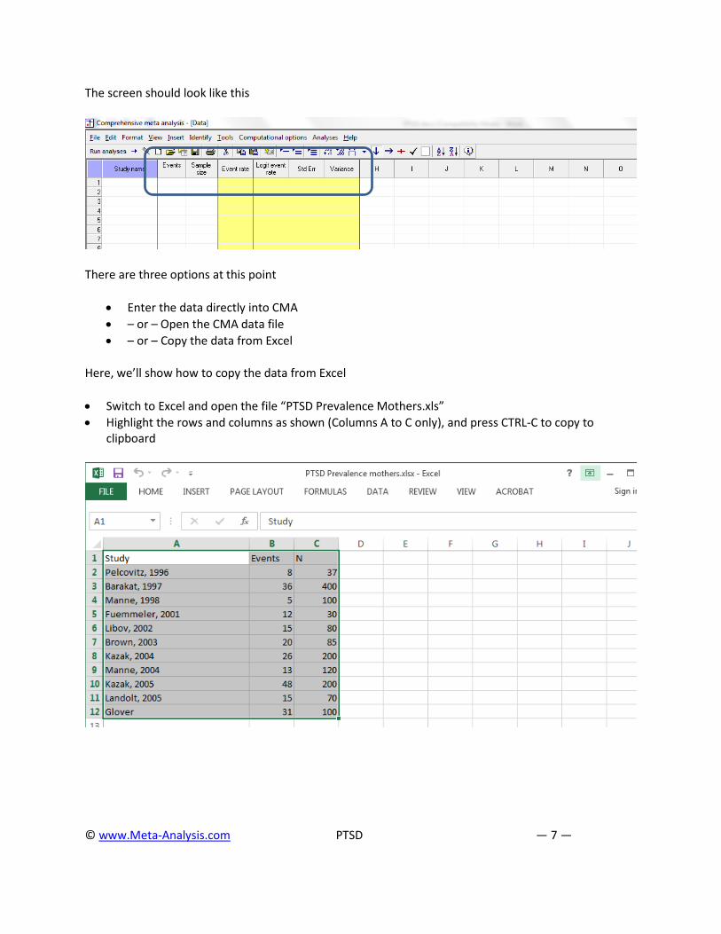
The screen should look like this
There are three options at this point
• Enter the data directly into CMA • – or – Open the CMA data file • – or – Copy the data from Excel
Here, we’ll show how to copy the data from Excel
• Switch to Excel and open the file “PTSD Prevalence Mothers.xls” • Highlight the rows and columns as shown (Columns A to C only), and press CTRL-C to copy to
clipboard

© www.Meta-Analysis.com PTSD — 8 —
• Switch to CMA • Click in cell Study-name 1 • Press [CTRL-V] to paste the data
At this point we should check that the data has been copied correctly
• Click anywhere in Row 1 • Select Edit > Delete row, and confirm
Click here
Click here
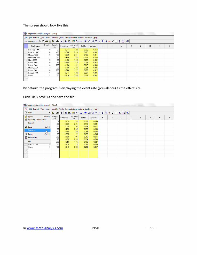
© www.Meta-Analysis.com PTSD — 9 —
The screen should look like this
By default, the program is displaying the event rate (prevalence) as the effect size
Click File > Save As and save the file

© www.Meta-Analysis.com PTSD — 10 —
Note that the file name is now in the header.
• [Save] will over-write the prior version of this file without warning • [Save As…] will allow you to save the file with a new name
To run the analysis, click [Run analysis]
© www.Meta-Analysis.com PTSD — 11 —
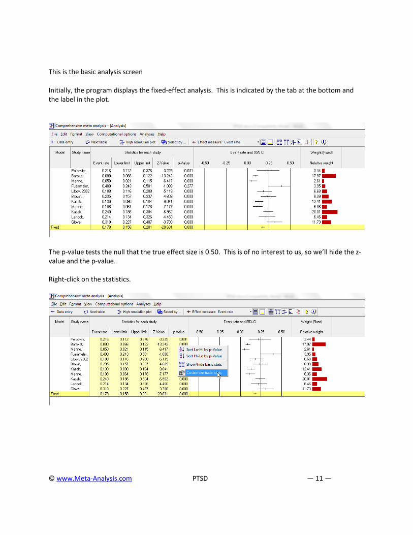
This is the basic analysis screen
Initially, the program displays the fixed-effect analysis. This is indicated by the tab at the bottom and the label in the plot.
The p-value tests the null that the true effect size is 0.50. This is of no interest to us, so we’ll hide the z-value and the p-value. Right-click on the statistics.

© www.Meta-Analysis.com PTSD — 12 —
• Remove check-marks for Z-value and p-value • Click Ok

© www.Meta-Analysis.com PTSD — 13 —
Click [Both models]
The program displays results for both the fixed-effect and the random-effects analysis.
Under the fixed-effect model the pooled estimate is 0.178, while under the random-effects model the pooled estimate is 0.180. While the estimate of prevalence happens to be almost identical under the two models, the precision of the estimate is very different.
• The fixed-effect model would be appropriate if all the studies were virtual replicates of each other. This is not the case here since the patients varied in important ways from study to study.
• The random-effects model would be appropriate if the studies vary in ways that may impact the effect size (such as those mentioned immediately above). Therefore, we will use the random-effects model.

© www.Meta-Analysis.com PTSD — 14 —
• Click Random on the tab at the bottom
The plot now displays the random-effects analysis alone.
A quick view of the plot suggests the following
The risk of PTSD varied substantially from study to study. The risks vary from a low of 5.0% to a high of 40.0% It seems that much of this variation reflects differences in real proportions The mean prevalence is 0.180 with a CI of 0.130 to 0.244

© www.Meta-Analysis.com PTSD — 15 —
Click [Next table]
Figure 1
The statistics at the left duplicate those we saw on the prior screen.
Under the random-effects model the mean prevalence is 0.180 with a 95% confidence interval of 0.130 to 0.244.
The statistics at the upper right relate to the dispersion of effect sizes across studies. The Q-value is 65.229 with df=10 and p< 0.001. Q reflects the distance of each study from the
mean effect (weighted, squared, and summed over all studies). Q is always computed using FE weights (which is the reason it is displayed on the “Fixed” row, but applies to both FE and RE analyses.
If all studies actually shared the same true effect size, the expected value of Q would be equal to df (which is 10). Here, Q is greater than that value, and so there is some evidence of variance in true effects. This excess variance falls outside the range that could be attributed to random variation in effects (it is statistically significant).
We had planned to use the random-effects model, since this matches the sampling frame for the studies, and would do so whether or not the Q-value was statistically significant.
T2 is the estimate of the between-study variance in true effects. This estimate is 0.346. T is the estimate of the between-study standard deviation in true effects. This estimate is 0.588. These value are both in logit units.
I2 reflects the proportion of true variance to observed variance. This is 84.669, which tells us that about 85% of the observed variance in effects is real. Put another way, if we were looking at a plot of the true effects rather than the observed effects, the variance in effects would be decreased by (1 minus .85) some 15%.
This high value of I2 tells us that if we could plot the true prevalence for each study, the dispersion would be only a little smaller than the dispersion we see in the plot of observed effects.
Click here
© www.Meta-Analysis.com PTSD — 16 —
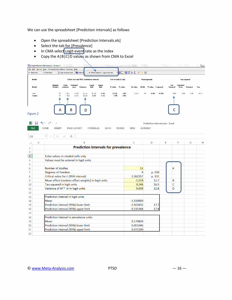
We can use the spreadsheet [Prediction intervals] as follows
• Open the spreadsheet [Prediction Intervals.xls] • Select the tab for [Prevalence] • In CMA select Logit event rate as the index • Copy the A|B|C|D values as shown from CMA to Excel
Figure 2
A B D C

© www.Meta-Analysis.com PTSD — 17 —
The confidence interval is 0.130 to 0.244 (read this from Figure 1, where the index is the event rate rather than the logit). The prediction interval (from Excel) is 0.051 to 0.471.
The true prevalence size varies from study to study. The mean prevalence probably falls in the range of 0.130 to 0.244. The true effect size for any single study will usually fall in the range of 0.051 to 0.471. In 95% of all possible meta-analyses, the true mean will fall in the range indicated by the CI. In 95% of all meta-analyses, 95% of all studies will fall inside the range indicated by the PI. This assumes that the true effect sizes are normally distributed.
• Click [Next table] to return to the main analysis screen • Click Hi-Resolution plot

© www.Meta-Analysis.com PTSD — 19 —
PTSD
Overview
This analysis includes eleven studies where mothers whose children suffered with chronic illnesses were evaluated for post-traumatic stress disorder (PTSD). Outcome was a diagnosis of PTSD, and the effect size is the prevalence of PTSD. The results of this analysis will be generalized to comparable studies, and so the random-effects model was employed for the analysis.
What is the pooled estimate of prevalence?
The pooled estimate of prevalence is 0.180, which means that on average about 18% of the mothers showed symptoms of PTSD. The confidence interval for the prevalence is 0.130 to 0.244, which tells us that the mean prevalence in the universe of comparable studies could fall anywhere in this range.
How much does the effect size vary across studies?
The Q-statistic provides a test of the null hypothesis that all studies in the analysis share a common effect size. If all studies shared the same effect size, the expected value of Q would be equal to the degrees of freedom (the number of studies minus 1). The Q-value is 65.229 with 10 degrees of freedom and p < 0.001. We can reject the null hypothesis that the true effect size is identical in all these studies. The I2 statistic is 85%, which tells us that 85% of the variance in observed effects reflects variance in true effects rather than sampling error. The variance of true effects in logit units (T2) is 0.346, and the standard deviation of true effects in logit units (T) is 0.588 [G]. If we assume that the prevalence is normally distributed (in logit units) we can estimate that the prediction interval is 0.051 to 0.471 [H] and predict that the true prevalence for any single population will usually fall in this range.
In this context, this is a broad range, and it would behoove us to understand why the prevalence varies so widely. For example, it may emerge that the prevalence depends on the child’s diseases. If we can identify the diseases associated with a higher prevalence of PTSD, we could target those communities for screening and assistance. Or, it could turn out that the prevalence depends on the support system available to the parents. In that case, we might want to devise strategies to provide additional support and reduce the prevalence of PTSD. What is clear from the prediction interval is that it would not be appropriate to focus on the mean prevalence of 18%, since this rate is not typical of many populations. Rather, we need to recognize that in any given population the prevalence could be substantially lower or higher than the mean.