EXAMINING THE WEAK FORM MARKET … THE WEAK FORM MARKET EFFICIENCY RISK: DETERMINANTS OF...
31
EXAMINING THE WEAK FORM MARKET EFFICIENCY RISK: DETERMINANTS OF MACROECONOMIC VARIABLES Abstract: This study investigates the weak form market efficiency of indices for the Financial, Industrial and Service returns as listed in the Muscat Securities Market (MSM30 index) in Oman, by conducting monthly observations from January 2010 until December 2014. All macroeconomic variables, covered under three sectoral indices, were found to be co- integrated. Furthermore, the findings exhibit that oil prices as a determinant have the most significant relationship on the three stock indices. The consumption price index (CPI) is the second most significant determinant revealed to impact the Service and Industrial indices prices, although it was found to exert no influence on the Financial index prices. Whilst inflation appears to be a third determinant, there is a significant effect on the Financial and Service indices prices, but no significant effect on the Industrial index prices. The overall findings from the period suggest that the Financial, Industrial and Service indices prices listed in MSM30 are inefficient in weak form market efficiency, which is consistent with previous studies examining the weak form of market efficiency. JEL classification: G32; G12 Keywords: Financial Risk; Efficiency; Oman; Capital Market; 1. INTRODUCTION After the 2008 stock market crash, the most considerable event to globally impact the stock market is the significant plunge in the price of crude oil, beginning in 2013. The per-barrel-pricing of crude dropped 50% in late 2014 (Bloomberg, 2015). Globally, this has had its effect on the international stock market, and from there, beyond, to other Financial, Service, and Industrial sectors, especially those of countries which are heavily reliant upon the economic contribution of crude oil to their gross domestic product (GDP). For Gulf Cooperation Council (GCC) countries, oil is the main economic 1 M., Head of Follow-Up and Settlement-Investment Department of the Public Authority for Social Insurance, Sultanate of Oman, Email: [email protected] 2* Corresponding author: K., College of Economics and Political Science, Sultan Qaboos University, Oman, Email: [email protected] IJER © Serials Publications 13(7), 2016: 3335-3365 ISSN: 0972-9380
Transcript of EXAMINING THE WEAK FORM MARKET … THE WEAK FORM MARKET EFFICIENCY RISK: DETERMINANTS OF...

EXAMINING THE WEAK FORM MARKETEFFICIENCY RISK: DETERMINANTS OFMACROECONOMIC VARIABLES
Abstract: This study investigates the weak form market efficiency of indices for the Financial,Industrial and Service returns as listed in the Muscat Securities Market (MSM30 index)in Oman, by conducting monthly observations from January 2010 until December 2014.
All macroeconomic variables, covered under three sectoral indices, were found to be co-integrated. Furthermore, the findings exhibit that oil prices as a determinant have the mostsignificant relationship on the three stock indices. The consumption price index (CPI) is thesecond most significant determinant revealed to impact the Service and Industrial indicesprices, although it was found to exert no influence on the Financial index prices. Whilstinflation appears to be a third determinant, there is a significant effect on the Financial andService indices prices, but no significant effect on the Industrial index prices.
The overall findings from the period suggest that the Financial, Industrial and Serviceindices prices listed in MSM30 are inefficient in weak form market efficiency, which isconsistent with previous studies examining the weak form of market efficiency.
JEL classification: G32; G12
Keywords: Financial Risk; Efficiency; Oman; Capital Market;
1. INTRODUCTION
After the 2008 stock market crash, the most considerable event to globally impact thestock market is the significant plunge in the price of crude oil, beginning in 2013. Theper-barrel-pricing of crude dropped 50% in late 2014 (Bloomberg, 2015). Globally, thishas had its effect on the international stock market, and from there, beyond, to otherFinancial, Service, and Industrial sectors, especially those of countries which are heavilyreliant upon the economic contribution of crude oil to their gross domestic product(GDP). For Gulf Cooperation Council (GCC) countries, oil is the main economic
1 M., Head of Follow-Up and Settlement-Investment Department of the Public Authority for SocialInsurance, Sultanate of Oman, Email: [email protected]
2* Corresponding author: K., College of Economics and Political Science, Sultan Qaboos University, Oman,Email: [email protected]
IJER © Serials Publications13(7), 2016: 3335-3365
ISSN: 0972-9380
3336 Mubarak Al-Habsi, and Khalid Al-Amri
contribution to the GDP. Using Oman as an example, the price of oil contributes to80% of Oman’s GDP (National Center for Statistics & Information, 2015).
Declining oil prices have impacted the investments of, and into, GCC financialmarkets, and GCC members find that their economies, and other Financial, Industrial,and Service sectors, are not immune to the effects of events such as falling oil prices,or severe crashes or slow-downs in markets and economies elsewhere in the world.Research by Sedik and William (2011) finds that the GCC stock markets are lessprotected against global crashes, as they are highly correlated. In fact, the MuscatSecurities Market1 (MSM30) index dropped over 7% in late 2014 as a result from thesharp fall of oil prices (Muscat Securities Market, 2015).
The MSM30 market has quite recently been improved and developed in terms ofthe corporate governance, market regularity, and disclosure over the last five years(Capital Market Authority, 2015). A solid trading and monitoring system, and increasedinformational transparency and disclosure, as well as the low price to earnings ratio(P/E) and cash dividends distributed by the listed companies in the MSM30 index,are theorized to be key factors towards securing stability in the MSM30 indexperformance. This could be surmised to have led to increased market efficiency.
Market inefficiency causes risk for two reasons, these being adverse selection andmoral hazard (Chepkoech Kemei, J., and Kenyatta, J., 2014). If there is no viableinformation on the averaging of insurance premiums, the less risky buyer hazardsborrowing at a higher rate than warranted by the actual market. Inaccurate informationleads the investor to invest or sell more heavily than actual performance of the marketwould warrant, had the investor proper knowledge of it (Langevoort, D., 2002). Havinglate or inaccurate information opens the investor up to chances of higher losses, as itenables the seller/lender to take greater than warranted risks with the buyer/investor’sfunds (Bernard, C., and Boyle, P., 2009; Langevoort, D., 2002). Also, having doctoredor falsified information means the seller may not put acquired funds to the best use,or even the intended use for those funds (Bernard, C., and Boyle, P., 2009; Hurt, C.,2010). In cases of falsified or doctored information, this is almost always at cost to theinvestor/buyer (Bernard, C., and Boyle, P., 2009; Hurt, C., 2010). Needless to say, lateinformation is of no use to the investor/buyer whatsoever (Bernard, C., and Boyle, P.,2009). For investors in the Bernard L. Madoff Investment Securities LL Cponzi schemefor example, the results of the simple quantitative diagnostics run by Bernard, C., andBoyle, P. (2009) would surely have raised suspicions about the firm’s performance. Ofcourse, would have, could have, and should have are no balm for the losses incurredby Madofff’s investors.
Abuse of information by agents in investment and lending organizations can gobeyond poor and minimal performance on stocks and individual investor andorganizational losses; systemic market inefficiency upsets the entire banking system,and as such, can lead to banks failing abruptly, creating inefficiencies on an economic-wide and, worryingly, global scale (Chepkoech Kemei, J., and Kenyatta, J., 2014). Of

Examining the weak form market efficiency risk... 3337
market inefficiency authors Chepkoech Kemei, J., and Kenyatta, J. conclude that“information asymmetries of capital markets constitute the backbone of financialineffectiveness and financial crisis” (2014, pp. 2). The purpose of this study is to examineweak form efficient market hypothesis (EMH) on three different sectors listed in theMSM30 index. These sectors are Financial, Industrial and Service, and they are observedin their entirety. This is done to determine the impact of macroeconomic variables,such as oil prices and other factors, on three sectoral indices. This has been done byconducting monthly analysis from the closing period of January, 2010, up untilDecember, 2014. We also observe whether or not the average returns on those indices,made on the historical time (days: t-1, t-2, t-3 and so on) are statistically significant ordifferent from today (t). Significance determines the impact of macroeconomic factorson the three sectoral indices prices volatility in a long-run relationship.
In the literature, to the best of our knowledge, there has been no attempt to assessthe weak form EMH in respect to main indices sectors prices (Financial, Industrialand Service) in their entirety. Among the three sectoral indices listed in MSM30,macroeconomic variables determinates instigate prices volatility. Differences representthe first major factor to justify further research concerning this market.
Another factor of relevance to researchers, stakeholders, and investors, is that themonthly analysis period selected (from 2010 to 2014) of this study is current and up todate, and uniquely focuses on the development of Oman’s stock market after the marketcrashes in 2008.
Additionally, this study demonstrates the market level in respect to the Financial,Service and Industrial sectors, in whether or not they are efficient.
Further, the study itself provides the rational for efficiencies and inefficiencies.
Finally, the previous, aids investment decisions2.
This study is organized as follows. Section 2 provides a review of the relevantliterature on weak form market efficiency and the existence of co-integrating vectorsand determinants. Section 3 represents the data used and Section 4 describes theresearch methodology. Section 5 provides all data analysis and our empirical results.Lastly, the conclusion of weak form market efficiency and determinates of the pricesimpact on the three sectoral indices is addressed in Section 6.
2. LITERATURE REVIEW
2.1. Capital Market Efficiency & Efficient Market Hypothesis
Capital market efficiency is described by researchers to exist in three forms: operational,allocative and informational efficiency (Fama, 1970; Alexander and Bailey, 1995;Muslumov, Aras, and Kurtulus, 2003Jones, 2007; Redhead, 2008;).
Efficient market hypothesis (EMH) embodies the form of informational efficiency.This form consists of the premise that all relevant information is immediately reflected
3338 Mubarak Al-Habsi, and Khalid Al-Amri
into current market prices and reflects the determination of the market value (Fama,1970). It refers to a perfect capital market, which assumes that all investors are rationaland have direct access to all available information, and that accessible informationand transactions are supposedly without costs. However, in real practice the marketparticipants are addressed to cover the transaction costs on their daily trading. EMHalso assumes that all stocks are fairly priced, and market participants will only be ableto earn a normal return on their stock prices, consistent with inherent market risk.
2.2. Approaches of Efficient Market Hypothesis
According to Fama (1970), the efficient market hypothesis (EMH) can be defined bydifferent approaches, each depending on the type of information revealed to investors.Types of information revealed to investors are often defined or groups as Weak-formefficient market hypothesis, Semi-strong form efficient market hypothesis and Strong-form efficient market hypothesis.
The Weak-form efficient market hypothesis suggests that current stock prices fullyincorporate all historical information, reflecting better estimates of intrinsic values(Malkiel, 1999). Hence, future prices cannot be predicted in advance based on thestudy of past stock prices. Thus, there is no benefit towards using technical analysis togain excessive stock returns if the market is weak form efficient. Conversely, rationalinvestors still have the opportunity to gain abnormal return on stock prices for valueand growth of stocks throughout their efforts of using fundamental analysis relativeto accounting measures such as earnings, cash flow, or book value (Dyckman andMorse, 1986). Dyckman and Morse (1986) demonstrate several tests of the marketefficient hypothesis to try weak form, which are the variance ratio, serial correlationdata, and the running of tests which include smaller unit root tests.
The Semi-strong form efficient market hypothesisposits that the current stock pricesfully reflect historical information, and are also reflective of the current availableinformation. This implies that analysts and investors cannot derive abnormal returnson stocks by implementing such information, because it includes corporate dividendannouncements, corporate announcements on merging and acquisitions, as well asspilt shares. However, fundamental analysis relative to accounting ratios such as bookvalue, earnings and cash flow can still be used by rational investors to achievesuccessive returns on stock prices. Fama (1991) has essentially validated this in theform of addressing several findings in respect to speed and the correspondence of theprice adjustments on the news about stock splits and earnings announcements. Findlayand Williams (2000) have found there is invalidity of achieving profitability byinvestors, since the relevant information and announcements were already reflectedinto the security prices at the time of announcements.
The Strong-form efficient hypothesisis that current available information, as wellas historical and private insider trading information reflects in the security prices atany given time. This implies that if the markets are strong form EMH, it would be
Examining the weak form market efficiency risk... 3339
pointless for investors to use technical, fundamental analysis or the most valuableinsider information which is available to top management to achieve abnormal returns.Penman (1982) points out that insider trading can achieve excessive returns on shareprices when buying shares before declaration, and selling stocks after theannouncement. As a result, insider trading groups have private information which isnot reflected in the stock prices.
2.3. Testing weak form EMH
The randomness test can be considerably examined by the weak form market efficientwhen implementing the weak form test, which demonstrates the independence ofprice changes at any given point of time. Bachelier (1900) has iterated that the stockprices directions and financial assets are weak form efficient in respect to the irrelevancyof historical prices’ movement with current financial securities prices.
Moreover, Fama (1965) examined market efficiency by implementing tests of serialcorrelation and running tests which generated daily data of approximately 30 stockslisted in the Dow Jones Industrial Average (DJIA) from 1956 to 1962. The findingswere not significantly different from zero, and illustrate very low correlation, leadingto the conclusion that the DJIA is efficient in weak form market efficiency. Perhaps,the research by Solnik (1973) points out that these markets diverge more from the‘Weak-form’ compared to what has been found in the United States. Nevertheless,correlation coefficient is low, which may suggest that when the correlation is zero byusing serial correlation and run tests, the market is considered to be efficient at theweak form of EMH.
On the other hand, Summers (1986) exhibits that the efficiency test of serialcorrelation can mislead the short term returns horizon. Despite, Fama and French(1988) have asserted that negative serial correlations at the short term horizon becomestronger as the return of the short term horizon increases. Moreover, the varianceratio and run tests methodology3 used by Abraham, Seyyed, and Alsakran (2002) haveemphasized, that upon implementing adjusted returns in Bahrain and Saudi Arabiacovering markets, the period from October 1992 and December 1998, these marketsare weak form EMH, and when using the raw data, these markets are inefficient inweak form EMH.
2.4. Testing weak form Market Efficiency in the MSM30 Index
Apart from the above research findings on testing weak form EMH, certain studiesconducted randomness tests on the MSM30 index.
Kharusi and Weagley (2014) they found that MSM30 index prices returns observeda positive correlation returns pre financial crisis (January 1, 2007 to June 8, 2008),whereas, a negative correlation for returns during the financial crisis from June 9,2008 to January 22, 2009 proceeded. Whilst, the results varied between positive andnegatives correlation returns on all index prices at post crisis levels from January 23,
3340 Mubarak Al-Habsi, and Khalid Al-Amri
2009 to January 17, 2011 the overacting result was that the MSM30 index during thefinancial crisis 2008 did not really follow the ‘Weak-form’ pattern, and thus it can belabeled inefficient during that period.
On the other hand one must not ignore a crucial study by Jawad (2011), found thaton monthly analysis reflect that the market is efficient in WFE. Whereas his finding ondaily analysis is that the market is inefficient in WFE. Arguably, Al-Jafari (2012) pointsout that the MSM is efficient and the market prices, and that stock returns areunpredictable in advance, as all available information is reflected more or less in thestock prices themselves.
2.5. The Impact of Macroeconomic variables on stock indices returns
Various empirical researchers have investigated the impacts of macroeconomicvariables on stock indices examines the influence of oil price changes on U.S stockindices prices with varied results, illustrating that the reaction of U.S stock indicesreturns may considerably fluctuate depending on the crude oil market. They returns.
An empirical study by Kilian and Park (2009) found insignificance of effect onstock indices returns relevant to the shocks of crude oil supply, whilst the positiveshocks of the demand on crude oil prices. Other studies by Jones and Kaul (1996), andKling (1985) report that declines of stock indices returns are correlated with increasesin crude oil prices, demonstrating a negative relationship.
Research by Park and Ratti (2008) explains that the negative relationship betweenthose variables exists on the oil importing countries, whilst the positive relationshipsubstantially exists on the oil exporting countries.
In contrast, Huang, Masulis, and Stoll (1996) have found no existence of a negativerelationship between stock returns and oil prices, which is in line with findings fromChen, Roll, and Ross (1986), who had previously suggested that the oil prices have noinfluence on stock returns. More recently, an empirical study by Cong et al. (2008),demonstrated4 that the shocks of crude oil prices had no significant impact on themajority of Chinese stock indices returns.
On the other hand, Yahyazadehfar and Babaie (2012) have used an auto regressionmodel (VAR) to examine the relationship between the macroeconomic variables andstock prices fluctuation. They point out that the Iranian stock prices and returnshave significant response on macroeconomic variables such as CPI, inflation, GDP,oil and gold prices. Additionally, several studies exhibit the influence of macro-economic factors on stock indices prices differently by implementing the Johansenco-integration test5, which represents the most common test methodology todetermine the relationship between those variables and the stock indices priceschanges.
From the literature is can be argued that the relationship between macroeconomicvariables and stock market indices partially reveals the informational market efficiency.

Examining the weak form market efficiency risk... 3341
3. DATA AND VARIABLE SELECTION
Initially, the data in this study is based on time series6. The data implemented hereinwas collected in May 2015. The method of data collection is based on secondaryinformation collected from two main financial institution sources, the Muscat SecuritiesMarket (MSM) and the National Center for statistics and information - DirectorateGeneral of Economic Statistics in Oman. The data was divided into two samples basedon the research purpose.
For the first sample, the data was obtained in the monthly closing prices for threemarket sectors in their entireties, which are the Financial, Service and Industrial indicesprices, as these are listed in the MSM30 index. They were collected for a period of fiveyears, from the closing period of January, 2010 to December, 2014. There werea totalof 60 observations. This was done to investigate whether the entire sectors listed inMSM30 follow a random walk and efficient in weak form market efficiency.
For the second sample, the data sought and captured firstly consisted of monthlymacroeconomic factors which are oil prices, CPI index (Consumer Price Index) andinflation rates as independent variables. Secondly, the three entire indices sectorsmonthly prices listed in MSM30 as dependent variables for five years from closingperiod of January, 2010 to December, 2014. There were a total of 60 observations. Thiswas done to investigate the significance of the impact of the macroeconomic factorson the return of the sectoral indices listed in MSM30.
Normally, the monthly closing which provides 60 observations are excluding theclosing, due to public holidays.
4. RESEARCH METHODOLOGY
Essentially, the prices of sectoral indices used to obtain the index returns. The followingequation was deployed:
Rt = [(P
t)/P
t–1] – 1 (1)
Where the:
Rt
– The daily returns of the index,
Pt
– Index price at time t,
Pt–1 – Index price at time t-1.
The correlation coefficient test is the statistical tool commonly used to indicatewhether or not there is randomness in indices prices changes. According to Gujarati(2012), the serial correlation coefficient known as autocorrelation test and it is definedas a measure of time series of returns and a different lagged period of the return withinthe same time series. Thus, autocorrelations accurately tests the independence anddependence of the random variables in a time series. Additionally, the former is calculatedby using the beta coefficient from the following estimated regression formula:
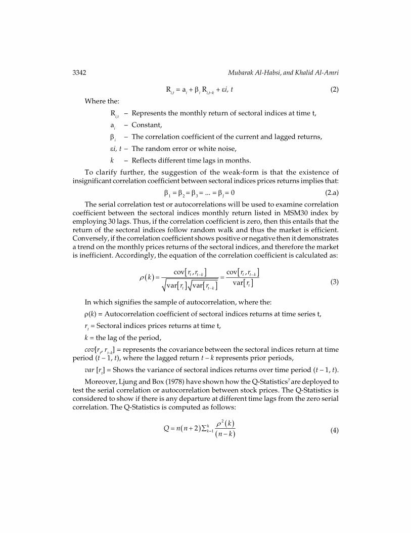
3342 Mubarak Al-Habsi, and Khalid Al-Amri
Ri,t = a
i + �
i R
i,t–k + �i, t (2)
Where the:
Ri,t
– Represents the monthly return of sectoral indices at time t,
ai
– Constant,
�i
– The correlation coefficient of the current and lagged returns,
�i, t – The random error or white noise,
k – Reflects different time lags in months.
To clarify further, the suggestion of the weak-form is that the existence ofinsignificant correlation coefficient between sectoral indices prices returns implies that:
�1 = �2 = �3 = ... = �J = 0 (2.a)
The serial correlation test or autocorrelations will be used to examine correlationcoefficient between the sectoral indices monthly return listed in MSM30 index byemploying 30 lags. Thus, if the correlation coefficient is zero, then this entails that thereturn of the sectoral indices follow random walk and thus the market is efficient.Conversely, if the correlation coefficient shows positive or negative then it demonstratesa trend on the monthly prices returns of the sectoral indices, and therefore the marketis inefficient. Accordingly, the equation of the correlation coefficient is calculated as:
� � � �� � � �
� �� �
� � �
�
� �cov , cov ,
varvar var
t tt k t k
tt t k
r r r rk
rr r (3)
In which signifies the sample of autocorrelation, where the:
�(k) = Autocorrelation coefficient of sectoral indices returns at time series t,
rt = Sectoral indices prices returns at time t,
k = the lag of the period,
cov[rt, r
t–k] = represents the covariance between the sectoral indices return at time
period (t – 1, t), where the lagged return t – k represents prior periods,
var [rt] = Shows the variance of sectoral indices returns over time period (t – 1, t).
Moreover, Ljung and Box (1978) have shown how the Q-Statistics7 are deployed totest the serial correlation or autocorrelation between stock prices. The Q-Statistics isconsidered to show if there is any departure at different time lags from the zero serialcorrelation. The Q-Statistics is computed as follows:
� � � �� ��
�� � ��
2
12 hk
kQ n n
n k (4)
Examining the weak form market efficiency risk... 3343
Where:
n – The sample size or number of observation,
h – Represents the number of lags,
pk – The sample serial correlation at lag k. whilst, n is number of observations,
Q – Statistic test is distributed from chi-squared with I degrees of freedom.
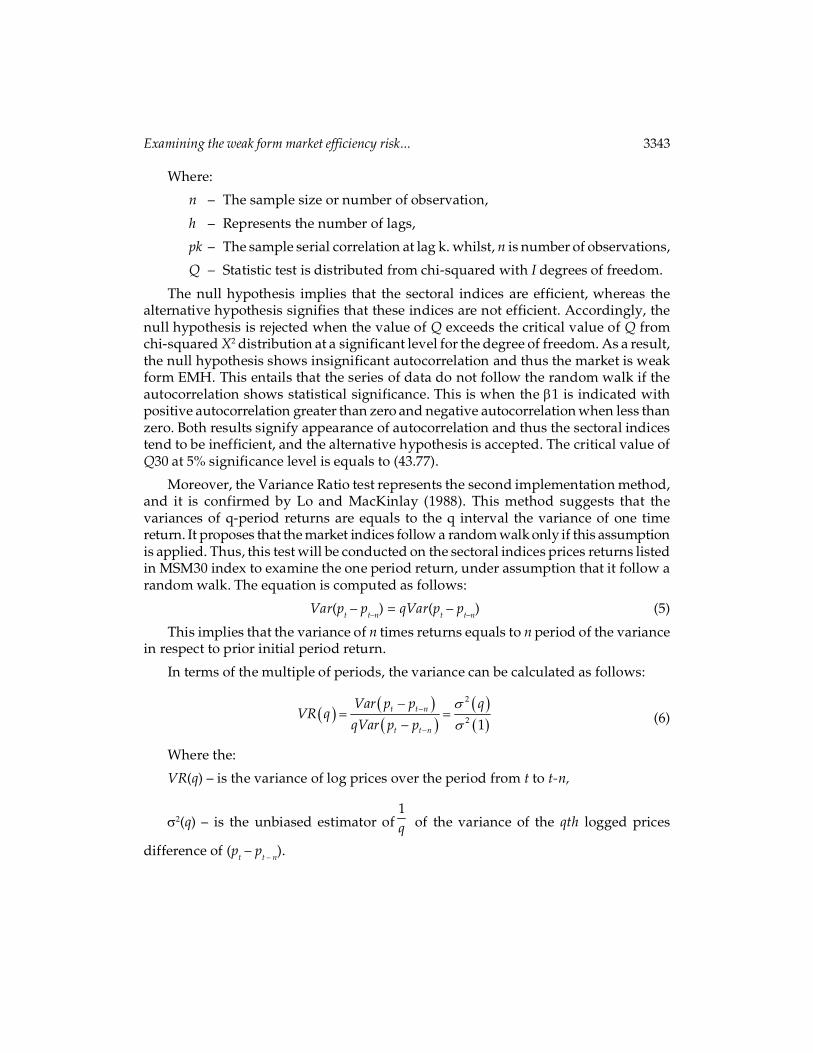
The null hypothesis implies that the sectoral indices are efficient, whereas thealternative hypothesis signifies that these indices are not efficient. Accordingly, thenull hypothesis is rejected when the value of Q exceeds the critical value of Q fromchi-squared X2 distribution at a significant level for the degree of freedom. As a result,the null hypothesis shows insignificant autocorrelation and thus the market is weakform EMH. This entails that the series of data do not follow the random walk if theautocorrelation shows statistical significance. This is when the �1 is indicated withpositive autocorrelation greater than zero and negative autocorrelation when less thanzero. Both results signify appearance of autocorrelation and thus the sectoral indicestend to be inefficient, and the alternative hypothesis is accepted. The critical value ofQ30 at 5% significance level is equals to (43.77).
Moreover, the Variance Ratio test represents the second implementation method,and it is confirmed by Lo and MacKinlay (1988). This method suggests that thevariances of q-period returns are equals to the q interval the variance of one timereturn. It proposes that the market indices follow a random walk only if this assumptionis applied. Thus, this test will be conducted on the sectoral indices prices returns listedin MSM30 index to examine the one period return, under assumption that it follow arandom walk. The equation is computed as follows:
Var(pt – p
t–n) = qVar(p
t – p
t–n) (5)
This implies that the variance of n times returns equals to n period of the variancein respect to prior initial period return.
In terms of the multiple of periods, the variance can be calculated as follows:
� � � �� �
� �� �
��
�
�
�� �
�
2
2 1t t n
t t n
Var p p qVR q
qVar p p (6)
Where the:
VR(q) – is the variance of log prices over the period from t to t-n,
�2(q) – is the unbiased estimator of1q of the variance of the qth logged prices
difference of (pt – p
t – n).

3344 Mubarak Al-Habsi, and Khalid Al-Amri
Thus, the null hypothesis for weak-form efficiency suggests that VR(q) = 1 for allq. Hence the null hypothesis is rejected when the VR is significantly different than 1which implies that if VR(q) > 1 then is it an indication of a positive serial correlation.According to Urrutia (1995), an existence of positive serial correlation is demonstratedin emerging markets, which indicates a growth signal of this market. On the otherhand, the indices returns show negative serial correlation if the null hypothesis isrejected and the VR(q) < 1. Fama and French (1998) have explained that this situationreflects market indices prices correction efficiently in developed markets. While,Summers (1986) has suggested that this an indication of economic and market bubblein the emerging markets.
Lo and MacKinlay (1988) have developed two test statistics hypothetical asymptoticdistribution over the estimated variance ratio. Thus, under assumption of nullhypothesis, the Z(q) represents the null hypothesis of homoscedasticity and Z*(q) isfor heteroscedasticity. Smith (2007) extolls that the validity of heteroscedasticity isused to examine the random walk hypothesis in the financial markets in respect toreturns volatility and time varying. Hence, if the null hypothesis is rejected, this mayindicate the existence of heteroscedasticity or autocorrelation. However, the return ofindices are serially correlated when the latter is rejected. The Z(q) and Z*(q) can becomputed as following equation:
� � � �� � � �� �� � � �1/22ˆ1 /Z q VR q s q (7)
� � � �� � � �� �� � � �1/2*2ˆ* 1 /Z q VR q s q (8)
Where the 2s and *2s are hypothetical asymptotic variances of the variance ratiotest under the assumptions of homoscedasticity and heteroscedasticity, respectively.
With characteristics of infrequent trading existing in the Muscat Securities market,and Oman being defined as a developing country, Miller, Muthuswamy, and Whaley’s(1994) recommendation for data adjustment for infrequent tradinghas been appliedso that the results might be more accurate. The adjustments of infrequent tradingdays has been devised by computing the residuals as following equation:
� � �� � ��0 1 1t t tR R (9)
Therefore, using this equation to calculate the adjusted returns of non-tradingdays as following:
� ���� �/ 1adjt tR (10)
In addition, this paper will further examine the existence of any Co-integrationequilibrium long-run relationship between the selected three macroeconomic variablesand the stock indices prices. Hence, this paper uses the Johansen co-integration test and
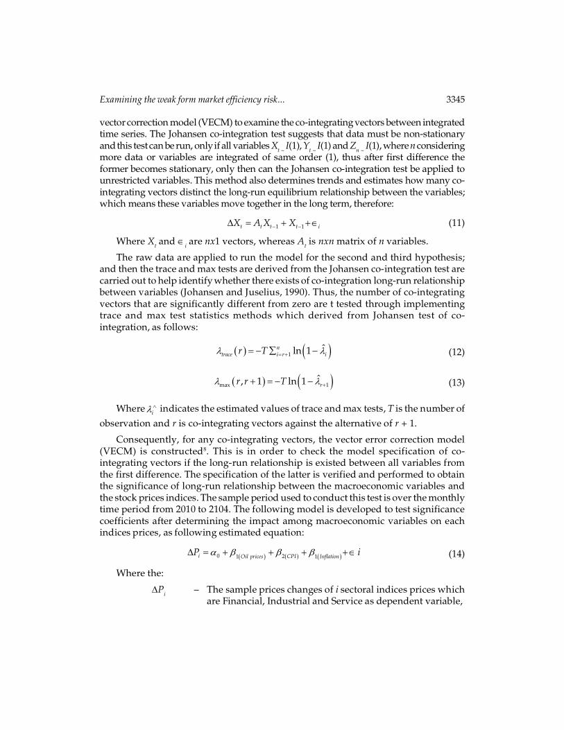
Examining the weak form market efficiency risk... 3345
vector correction model (VECM) to examine the co-integrating vectors between integratedtime series. The Johansen co-integration test suggests that data must be non-stationaryand this test can be run, only if all variables X
t ~ I(1), Y
t ~ I(1) and Z
n ~ I(1), where n considering
more data or variables are integrated of same order (1), thus after first difference theformer becomes stationary, only then can the Johansen co-integration test be applied tounrestricted variables. This method also determines trends and estimates how many co-integrating vectors distinct the long-run equilibrium relationship between the variables;which means these variables move together in the long term, therefore:
� �� � � ��1 1t t t t iX A X X (11)
Where Xt and �
i are nx1 vectors, whereas A
t is nxn matrix of n variables.
The raw data are applied to run the model for the second and third hypothesis;and then the trace and max tests are derived from the Johansen co-integration test arecarried out to help identify whether there exists of co-integration long-run relationshipbetween variables (Johansen and Juselius, 1990). Thus, the number of co-integratingvectors that are significantly different from zero are t tested through implementingtrace and max test statistics methods which derived from Johansen test of co-integration, as follows:
� � � �� �� �� � � �1ˆln 1n
trace i r ir T (12)
� � � �� � �� � � �max 1ˆ, 1 ln 1 rr r T (13)
Where��i indicates the estimated values of trace and max tests, T is the number of
observation and r is co-integrating vectors against the alternative of r + 1.
Consequently, for any co-integrating vectors, the vector error correction model(VECM) is constructed8. This is in order to check the model specification of co-integrating vectors if the long-run relationship is existed between all variables fromthe first difference. The specification of the latter is verified and performed to obtainthe significance of long-run relationship between the macroeconomic variables andthe stock prices indices. The sample period used to conduct this test is over the monthlytime period from 2010 to 2104. The following model is developed to test significancecoefficients after determining the impact among macroeconomic variables on eachindices prices, as following estimated equation:
� � � � � �� � � �� � � � � ��0 21 1i CPIOil prices InflationP i (14)
Where the:
�Pi
– The sample prices changes of i sectoral indices prices whichare Financial, Industrial and Service as dependent variable,

3346 Mubarak Al-Habsi, and Khalid Al-Amri
�0 – Represents the constant,
�1 (Oil prices) = The slop or correlation coefficient for the oil prices as anindependent variable,
�2 (CPI) = The slop or correlation coefficient for the CPI as anindependent variable,
�1 (Inflation) = The slop or correlation coefficient for the inflation as anindependent variable,
�i = The error term or residuals.
Correspondingly, the data is plotted based on the logarithmic scale, so that allvariables are converted into natural logarithm; the reason is based on monthly statistics,all indices returns data are estimated. Gujarati (2014) has suggested this approach inorder reduce the gap among the variables. Hence, the model considered for regression,is as follows:
� � � � � �� � � �� � � � � ��0 1 2 1 iLn P Ln oil prices Ln CPI inflation i (15)
Where Ln = the natural logarithm.
Therefore, the elasticities of estimated coefficients for the long run relationshipbetween variables can be interpreted, since the four variables are transferred to naturallogarithm.
5. RESULTS AND DISCUSSION
5.1. Descriptive Statistics
Table 1 presents the summary of descriptive statistics for all stock returns indicessectors listed in MSM30 index and macroeconomic variables, for the monthly sampleperiod from January 2010 to December 2014. The number of observations is 60 foreach variable. It shows that Financial Index return and inflation have negative meanof -0.2% and nearly -15%, correspondingly. The returns of Industrial and Serviceindices, as well as oil prices and CPI have a positive mean of 0.3%, 0.5%, 0.3% and0.1%, respectively. The mean of all variables are very close to the median, which denotesthere is no existence of outliers within the data. Thus, the mean is surmised to be anunbiased estimator for these variables. The monthly returns dispersion is measuredby the standard deviation, which indicates how possible rates of return are volatilearound the expected rate of return.
The Service sector index has the lowest standard deviation of approximately 4%compare to Financial and Industrial indices with nearly 5% and 4%, respectively. Thisimplies that the Service sector index has a low risk compared to other indices sectors.
On the other hand, the outcome indicates that the oil prices variable has a positivemean return of 0.3%, while CPI and inflation have a positive of 0.1% and nearly negative
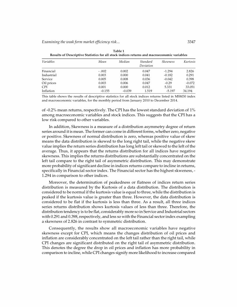
Examining the weak form market efficiency risk... 3347
of -0.2% mean returns, respectively. The CPI has the lowest standard deviation of 1%among macroeconomic variables and stock indices. This suggests that the CPI has alow risk compared to other variables.
In addition, Skewness is a measure of a distribution asymmetry degree of returnseries around it is mean. The former can come in different forms, whether zero, negativeor positive. Skewness of normal distribution is zero, whereas positive value of skewmeans the data distribution is skewed to the long right tail, while the negative skewvalue implies the return series distribution has long left tail or skewed to the left of theaverage. Thus, it appears that the returns distribution for all indices have negativeskewness. This implies the returns distributions are substantially concentrated on theleft tail compare to the right tail of asymmetric distribution. This may demonstratemore probability of significant decline in indices returns compare to incline in returns,specifically in Financial sector index. The Financial sector has the highest skweness, -1.294 in comparison to other indices.
Moreover, the determination of peakedness or flatness of indices return seriesdistribution is measured by the Kurtosis of a data distribution. The distribution isconsidered to be normal if the kurtosis value is equal to three, while the distribution ispeaked if the kurtosis value is greater than three. However, the data distribution isconsidered to be flat if the kurtosis is less than three. As a result, all three indicesseries returns distribution shows kurtosis values of less than three. Therefore, thedistribution tendency is to be flat, considerably more so in Service and Industrial sectorswith 0.291 and 0.398, respectively, and less so with the Financial sector index examplinga skewness of 2.826 in contrast to symmetric distribution.
Consequently, the results show all macroeconomic variables have negativeskewness except for CPI, which means the changes distribution of oil prices andinflation are considerably concentrated on the left tail rather than the right tail, whileCPI changes are significant distributed on the right tail of asymmetric distribution.This denotes the degree the drop in oil prices and inflation has more probability incomparison to incline, while CPI changes signify more likelihood to increase compared
Table 1Results of Descriptive Statistics for all stock indices returns and macroeconomic variables
Variables Mean Median Standard Skewness KurtosisDeviation
Financial - .002 0.002 0.047 -1.294 2.826Industrial 0.003 0.000 0.041 -0.182 0.291Service 0.005 0.008 0.036 -0.042 0.398Oil prices 0.003 0.006 0.047 -0.29 -0.072CPI 0.001 0.000 0.012 5.331 33.051Inflation -0.155 -0.039 1.519 -5.197 34.194
This table shows the results of descriptive statistics for all stock indices returns listed in MSM30 indexand macroeconomic variables, for the monthly period from January 2010 to December 2014.

3348 Mubarak Al-Habsi, and Khalid Al-Amri
to decline. Additionally, all three macroeconomic variables show kurtosis valuessignificantly more than three, except for oil prices. Hence, the distribution tendencyto be substantially peaked in CPI and inflation, whilst flatter on oil prices in contrastto symmetric distribution.
5.2. Results of monthly Serial Correlation Test for Financial Sector Index
Table 2 contains the results of the serial correlation test up to 30 lags using monthlyarithmetic return of the Financial sector index over the period from January 2010 toDecember 2014.
The basic assumption is that the null hypothesis of weak form EMH is rejected ifthe Financial index returns are serially correlated. Thus, all lags correlation coefficientsare not statistically significant at the 5% significant level in Financial sector index exceptfor lags 10 and 20 are statistically significant at 10%.
Table 2Results of monthly Serial Correlation Test for Financial Sector Index
Lags AC Q-Stat Probability
1 -.0.017 0.018 0.8972 -0.034 0.083 0.8053 0.143 1.171 0.3154 0.029 1.191 0.8415 -0.113 1.864 0.4406 0.115 2.938 0.4417 -0.088 3.233 0.5638 0.199 4.620 0.1959 0.193 6.612 0.121
10 -0.279 10.465 *0.075115 -0.199 11.732 0.23820 -0.347 16.923 *0.061725 -0.323 23.032 0.13330 0.088 27.188 0.719
This table shows the results of autocorrelation test for Financial Sector Index returns up to 30 lags usingmonthly arithmetic return using Ljung and Box (1978) Q-Statistics for the period of January 2010 toDecember 2014. The *, **, *** represents the significance at 10, 5, and 1 per cent significance levelsrespectively.
Hence, the significance at 5% level of AC coefficients shows that the index returnsseries exhibit serial independence for all intervals. Thus, the null hypothesis of randomwalk is accepted. In this particular sample, the tendency of serial dependence for theselags shows the returns cannot be easily used to predict the future returns. On theother hand, the Q-Statistics exhibit that all Q values for all lags are lower than thecritical value of 43.77. Thereby they are inside critical interval. Therefore, the Q-statisticsconfirm that the lags from 1 to 30 fail to reject the null hypothesis and thus the Financialindex return has no autocorrelation. As a result, the Financial index return is efficientin efficient market hypothesis.
Examining the weak form market efficiency risk... 3349
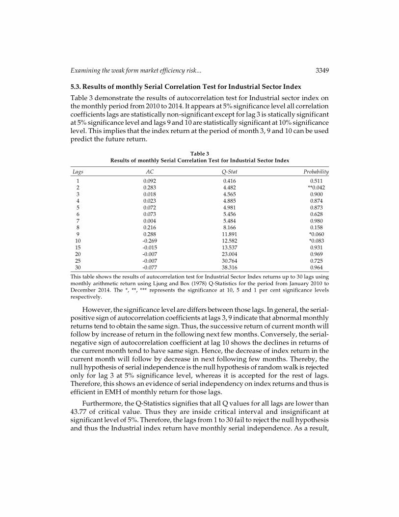
5.3. Results of monthly Serial Correlation Test for Industrial Sector Index
Table 3 demonstrate the results of autocorrelation test for Industrial sector index onthe monthly period from 2010 to 2014. It appears at 5% significance level all correlationcoefficients lags are statistically non-significant except for lag 3 is statically significantat 5% significance level and lags 9 and 10 are statistically significant at 10% significancelevel. This implies that the index return at the period of month 3, 9 and 10 can be usedpredict the future return.
Table 3Results of monthly Serial Correlation Test for Industrial Sector Index
Lags AC Q-Stat Probability
1 0.092 0.416 0.5112 0.283 4.482 **0.0423 0.018 4.565 0.9004 0.023 4.885 0.8745 0.072 4.981 0.8736 0.073 5.456 0.6287 0.004 5.484 0.9808 0.216 8.166 0.1589 0.288 11.891 *0.060
10 -0.269 12.582 *0.08315 -0.015 13.537 0.93120 -0.007 23.004 0.96925 -0.007 30.764 0.72530 -0.077 38.316 0.964
This table shows the results of autocorrelation test for Industrial Sector Index returns up to 30 lags usingmonthly arithmetic return using Ljung and Box (1978) Q-Statistics for the period from January 2010 toDecember 2014. The *, **, *** represents the significance at 10, 5 and 1 per cent significance levelsrespectively.
However, the significance level are differs between those lags. In general, the serial-positive sign of autocorrelation coefficients at lags 3, 9 indicate that abnormal monthlyreturns tend to obtain the same sign. Thus, the successive return of current month willfollow by increase of return in the following next few months. Conversely, the serial-negative sign of autocorrelation coefficient at lag 10 shows the declines in returns ofthe current month tend to have same sign. Hence, the decrease of index return in thecurrent month will follow by decrease in next following few months. Thereby, thenull hypothesis of serial independence is the null hypothesis of random walk is rejectedonly for lag 3 at 5% significance level, whereas it is accepted for the rest of lags.Therefore, this shows an evidence of serial independency on index returns and thus isefficient in EMH of monthly return for those lags.
Furthermore, the Q-Statistics signifies that all Q values for all lags are lower than43.77 of critical value. Thus they are inside critical interval and insignificant atsignificant level of 5%. Therefore, the lags from 1 to 30 fail to reject the null hypothesisand thus the Industrial index return have monthly serial independence. As a result,

3350 Mubarak Al-Habsi, and Khalid Al-Amri
the Financial index return follow random walk and is efficient in efficient markethypothesis. This implies the current month of index return cannot be easily used topredict future index returns.
5.4. Results of monthly Serial Correlation Test for Service Sector Index
Table 4 determines the results of monthly serial correlation test for Service sector indexfor the period from 2010 to 2014. This indicates that all lags coefficients at 5%significance level are statically non-significant except for lag 5 is statically significantat 1% significance level. This suggests that the index return at the period of month 5can be used to predict the future return at only the 1% significance level. Generally,the serial-negative sign of autocorrelation coefficient at lag 5 exhibit the decrease inreturns of the current month tend to result same sign. Hence, the decline of indexreturn in the month 5th expected to fall in next following few months. Thus, the indexreturn at lag 5 have autocorrelation and it is not random. Therefore the null hypothesisof serial independence is rejected at 1% significance level. Thereby, this provides anevidence of serial dependency on index returns and thus is not efficient in EMH ofmonthly return on this lag. Whilst, the serial correlation of the index returns aresubstantially shows non-significant for all monthly intervals at 5% significance level.This suggests that these intervals fail to reject the null hypothesis and the Serviceindex is efficient in EMH.
Table 4Results of monthly Serial Correlation Test for Service Sector Index
Lags AC Q-Stat Probability
1 -0.099 0.612 0.4522 0.097 1.311 0.4703 0.164 2.421 0.2324 -0.067 2.896 0.6295 -0.367 7.996 ***0.0086 0.041 8.913 0.7777 0.035 9.853 0.8108 0.113 9.880 0.4499 -0.035 9.939 0.815
10 -0.073 9.984 0.63315 0.086 11.417 0.59620 -0.133 19.294 0.46725 -0.200 21.198 0.34530 -0.132 22.286 0.579
This table shows the results of autocorrelation test for Service Sector Index returns up to 30 lags usingmonthly arithmetic return using Ljung and Box (1978) Q-Statistics for the period from January 2010 toDecember 2014. The *, **, *** represents the significance at 10, 5 and 1 per cent significance levels,respectively.
The Q-Statistics indicates that the critical value 43.77 is greater than the Q values forall lags. Thus, the latter are inside critical interval and thereby non-significant at significant

Examining the weak form market efficiency risk... 3351
level of 5%. Therefore, the Q-Statistics confirm the autocorrelation does not exists forthe monthly lags from 1 to 30 and null hypothesis is rejected. Hence, the Service sectorindex follow random walk and is efficient in efficient market hypothesis. Thisdemonstrates of inability to predict the future index returns using the historical lags.
5.5. Results of monthly Variance Ratio Test for Financial Sector Index
Table 5 determines the results of the monthly variance ratio test up to 25 lag ordersusing of Financial sector index returns under assumptions of homoskedasticity andheteroskedasticity, which are presented for the sample the period of January 2010 toDecember 2014. Correspondingly, the null hypothesis of weak form EMH is rejected ifthe variance rations of Financial index returns are different than one under thoseassumption. Thus, it demonstrates from the results of variance ratio test underassumption homoscedasticity that z-statistics shows the values of (q) at 5% significancelevel are considerably different than one for all lags 6, 8 and 9, and for lags 4, 5, 6 underassumption of heteroskedasticity. Therefore, under both assumption, the null hypothesisis failed to be accepted for Financial sector index, which signifies the returns is seriallycorrelated and it does not follow a random walk process. The rejection of random walkprocess due to the monthly index returns suffers from heteroskedasticity andautocorrelation. Thus, the index is inefficient in efficient market hypothesis.
Table 5Results of monthly Variance Ratio Test for Financial Sector Index
Homoskedasticity HeteroskedasticityLags Variance Ratio Z-Statistics Probability Z-Statistics Probability
2 0.509 -3.737 ***0.000 -2.673 ***0.0073 0.277 -3.659 ***0.000 -2.790 ***0.0054 0.238 -3.046 ***0.002 -2.291 **0.0225 0.212 -2.655 ***0.008 -2.079 **0.0386 0.141 -2.553 **0.011 -2.067 **0.0397 0.171 -2.275 0.229 -1.866 *0.0628 0.118 -2.230 **0.023 -1.820 *0.0699 0.096 -2.093 **0.036 -1.414 0.157
10 0.155 -1.770 *0.077 -1.606 0.10815 0.082 -1.449 0.147 -1.414 0.15420 0.075 -1.177 0.239 -1.214 0.22525 0.081 -1.160 0.246 -1.153 0.249
This table shows the results of monthly variance ratio test for Financial Sector Index returns, conductedup to 25 lag orders using Lo and MacKinlay (1988) under homoskedasticity and heteroskedasticity, forthe period from January 2010 to December 2014. The *, **, *** represents the significance at 10, 5 and 1 percent significance levels respectively.
5.6. Results of monthly Variance Ratio Test for Industrial Sector Index
Table 6 presents the results of the monthly variance ratio test performed up to 25lag orders. The returns for the sample period from January 2010 to December 2014is used to perform the variance ratio test for Financial sector index under
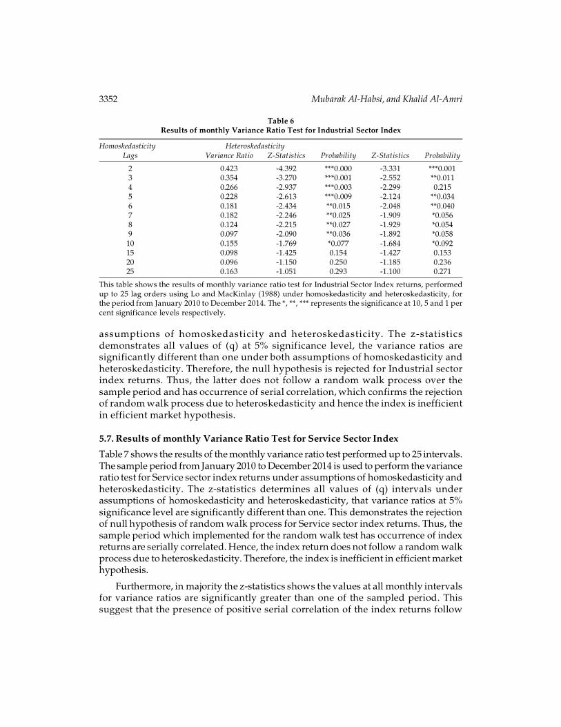
3352 Mubarak Al-Habsi, and Khalid Al-Amri
assumptions of homoskedasticity and heteroskedasticity. The z-statisticsdemonstrates all values of (q) at 5% significance level, the variance ratios aresignificantly different than one under both assumptions of homoskedasticity andheteroskedasticity. Therefore, the null hypothesis is rejected for Industrial sectorindex returns. Thus, the latter does not follow a random walk process over thesample period and has occurrence of serial correlation, which confirms the rejectionof random walk process due to heteroskedasticity and hence the index is inefficientin efficient market hypothesis.
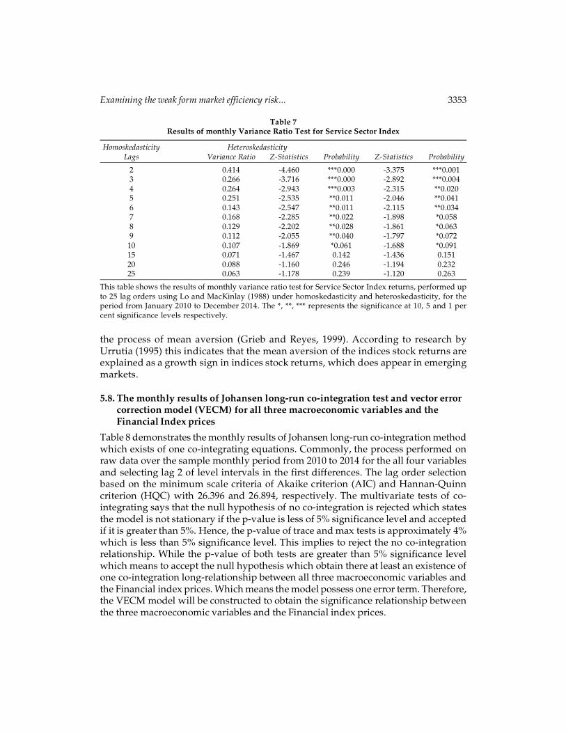
5.7. Results of monthly Variance Ratio Test for Service Sector Index
Table 7 shows the results of the monthly variance ratio test performed up to 25 intervals.The sample period from January 2010 to December 2014 is used to perform the varianceratio test for Service sector index returns under assumptions of homoskedasticity andheteroskedasticity. The z-statistics determines all values of (q) intervals underassumptions of homoskedasticity and heteroskedasticity, that variance ratios at 5%significance level are significantly different than one. This demonstrates the rejectionof null hypothesis of random walk process for Service sector index returns. Thus, thesample period which implemented for the random walk test has occurrence of indexreturns are serially correlated. Hence, the index return does not follow a random walkprocess due to heteroskedasticity. Therefore, the index is inefficient in efficient markethypothesis.
Furthermore, in majority the z-statistics shows the values at all monthly intervalsfor variance ratios are significantly greater than one of the sampled period. Thissuggest that the presence of positive serial correlation of the index returns follow
Table 6Results of monthly Variance Ratio Test for Industrial Sector Index
Homoskedasticity HeteroskedasticityLags Variance Ratio Z-Statistics Probability Z-Statistics Probability
2 0.423 -4.392 ***0.000 -3.331 ***0.0013 0.354 -3.270 ***0.001 -2.552 **0.0114 0.266 -2.937 ***0.003 -2.299 0.2155 0.228 -2.613 ***0.009 -2.124 **0.0346 0.181 -2.434 **0.015 -2.048 **0.0407 0.182 -2.246 **0.025 -1.909 *0.0568 0.124 -2.215 **0.027 -1.929 *0.0549 0.097 -2.090 **0.036 -1.892 *0.058
10 0.155 -1.769 *0.077 -1.684 *0.09215 0.098 -1.425 0.154 -1.427 0.15320 0.096 -1.150 0.250 -1.185 0.23625 0.163 -1.051 0.293 -1.100 0.271
This table shows the results of monthly variance ratio test for Industrial Sector Index returns, performedup to 25 lag orders using Lo and MacKinlay (1988) under homoskedasticity and heteroskedasticity, forthe period from January 2010 to December 2014. The *, **, *** represents the significance at 10, 5 and 1 percent significance levels respectively.
Examining the weak form market efficiency risk... 3353
the process of mean aversion (Grieb and Reyes, 1999). According to research byUrrutia (1995) this indicates that the mean aversion of the indices stock returns areexplained as a growth sign in indices stock returns, which does appear in emergingmarkets.
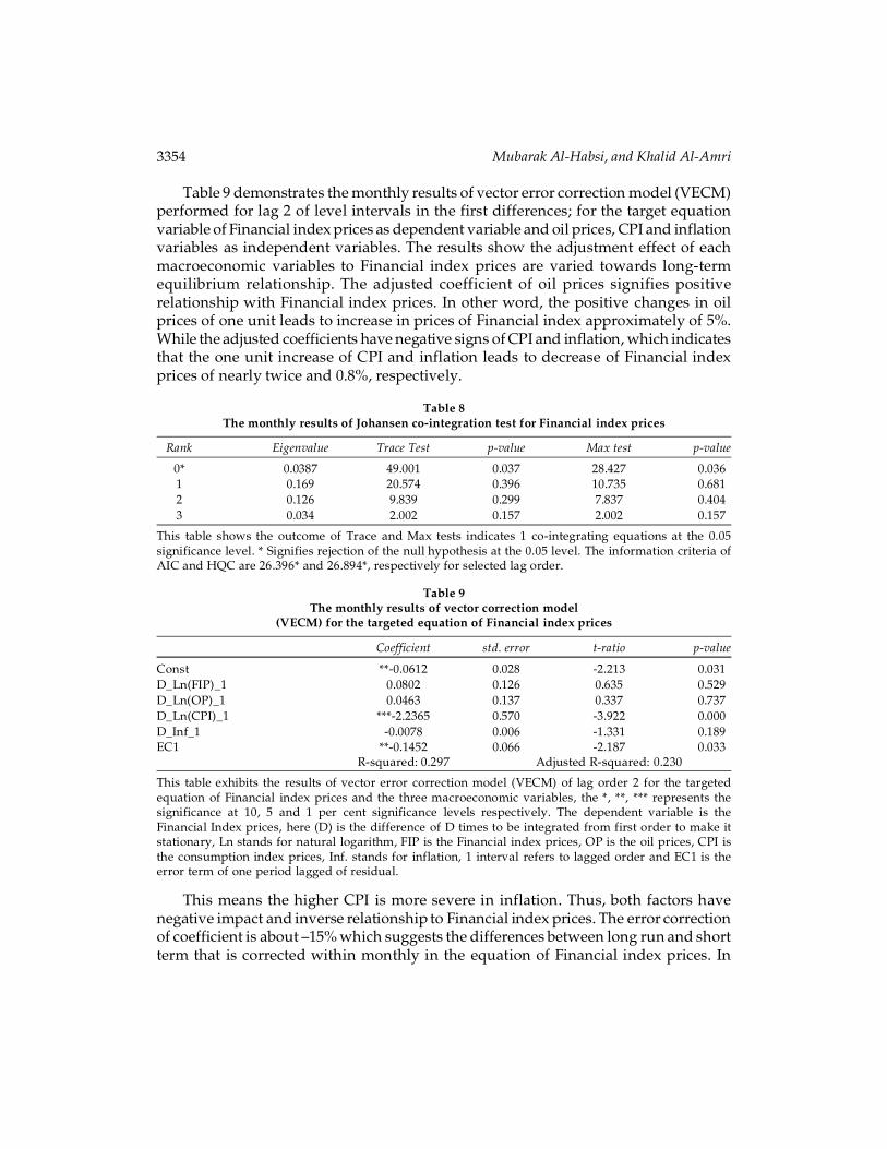
5.8. The monthly results of Johansen long-run co-integration test and vector errorcorrection model (VECM) for all three macroeconomic variables and theFinancial Index prices
Table 8 demonstrates the monthly results of Johansen long-run co-integration methodwhich exists of one co-integrating equations. Commonly, the process performed onraw data over the sample monthly period from 2010 to 2014 for the all four variablesand selecting lag 2 of level intervals in the first differences. The lag order selectionbased on the minimum scale criteria of Akaike criterion (AIC) and Hannan-Quinncriterion (HQC) with 26.396 and 26.894, respectively. The multivariate tests of co-integrating says that the null hypothesis of no co-integration is rejected which statesthe model is not stationary if the p-value is less of 5% significance level and acceptedif it is greater than 5%. Hence, the p-value of trace and max tests is approximately 4%which is less than 5% significance level. This implies to reject the no co-integrationrelationship. While the p-value of both tests are greater than 5% significance levelwhich means to accept the null hypothesis which obtain there at least an existence ofone co-integration long-relationship between all three macroeconomic variables andthe Financial index prices. Which means the model possess one error term. Therefore,the VECM model will be constructed to obtain the significance relationship betweenthe three macroeconomic variables and the Financial index prices.
Table 7Results of monthly Variance Ratio Test for Service Sector Index
Homoskedasticity HeteroskedasticityLags Variance Ratio Z-Statistics Probability Z-Statistics Probability
2 0.414 -4.460 ***0.000 -3.375 ***0.0013 0.266 -3.716 ***0.000 -2.892 ***0.0044 0.264 -2.943 ***0.003 -2.315 **0.0205 0.251 -2.535 **0.011 -2.046 **0.0416 0.143 -2.547 **0.011 -2.115 **0.0347 0.168 -2.285 **0.022 -1.898 *0.0588 0.129 -2.202 **0.028 -1.861 *0.0639 0.112 -2.055 **0.040 -1.797 *0.072
10 0.107 -1.869 *0.061 -1.688 *0.09115 0.071 -1.467 0.142 -1.436 0.15120 0.088 -1.160 0.246 -1.194 0.23225 0.063 -1.178 0.239 -1.120 0.263
This table shows the results of monthly variance ratio test for Service Sector Index returns, performed upto 25 lag orders using Lo and MacKinlay (1988) under homoskedasticity and heteroskedasticity, for theperiod from January 2010 to December 2014. The *, **, *** represents the significance at 10, 5 and 1 percent significance levels respectively.
3354 Mubarak Al-Habsi, and Khalid Al-Amri
Table 9 demonstrates the monthly results of vector error correction model (VECM)performed for lag 2 of level intervals in the first differences; for the target equationvariable of Financial index prices as dependent variable and oil prices, CPI and inflationvariables as independent variables. The results show the adjustment effect of eachmacroeconomic variables to Financial index prices are varied towards long-termequilibrium relationship. The adjusted coefficient of oil prices signifies positiverelationship with Financial index prices. In other word, the positive changes in oilprices of one unit leads to increase in prices of Financial index approximately of 5%.While the adjusted coefficients have negative signs of CPI and inflation, which indicatesthat the one unit increase of CPI and inflation leads to decrease of Financial indexprices of nearly twice and 0.8%, respectively.
Table 8The monthly results of Johansen co-integration test for Financial index prices
Rank Eigenvalue Trace Test p-value Max test p-value
0* 0.0387 49.001 0.037 28.427 0.0361 0.169 20.574 0.396 10.735 0.6812 0.126 9.839 0.299 7.837 0.4043 0.034 2.002 0.157 2.002 0.157
This table shows the outcome of Trace and Max tests indicates 1 co-integrating equations at the 0.05significance level. * Signifies rejection of the null hypothesis at the 0.05 level. The information criteria ofAIC and HQC are 26.396* and 26.894*, respectively for selected lag order.
Table 9The monthly results of vector correction model
(VECM) for the targeted equation of Financial index prices
Coefficient std. error t-ratio p-value
Const **-0.0612 0.028 -2.213 0.031D_Ln(FIP)_1 0.0802 0.126 0.635 0.529D_Ln(OP)_1 0.0463 0.137 0.337 0.737D_Ln(CPI)_1 ***-2.2365 0.570 -3.922 0.000D_Inf_1 -0.0078 0.006 -1.331 0.189EC1 **-0.1452 0.066 -2.187 0.033
R-squared: 0.297 Adjusted R-squared: 0.230
This table exhibits the results of vector error correction model (VECM) of lag order 2 for the targetedequation of Financial index prices and the three macroeconomic variables, the *, **, *** represents thesignificance at 10, 5 and 1 per cent significance levels respectively. The dependent variable is theFinancial Index prices, here (D) is the difference of D times to be integrated from first order to make itstationary, Ln stands for natural logarithm, FIP is the Financial index prices, OP is the oil prices, CPI isthe consumption index prices, Inf. stands for inflation, 1 interval refers to lagged order and EC1 is theerror term of one period lagged of residual.
This means the higher CPI is more severe in inflation. Thus, both factors havenegative impact and inverse relationship to Financial index prices. The error correctionof coefficient is about –15% which suggests the differences between long run and shortterm that is corrected within monthly in the equation of Financial index prices. In

Examining the weak form market efficiency risk... 3355
which, this signifies a modest rate of adjustments to the long term balance relationshipamong variables. On the other hand, the results determines that the oil prices havesignificant effect on the Financial index prices, that is because of p-value of oil pricesfactor equals to 74% is significantly greater than 5% significance level. Consideringthe p-value of the inflation factor is statistically significant at 5% significance level,which implies that this factor has strong relationship to the Financial index prices, butless compared to the factor of oil prices.
Whereas, the p-values of CPI shows less than 5% significance level which meanthat CPI is non-significant at 5% significance level, which implies the null hypothesisfor lag 2 is rejected for the CPI and accepted for the oil prices and inflation factors.Furthermore, this specifies that Financial index prices is considerably affected andhas significant impact by oil prices in comparison to the inflation factor, whilst CPIfactor have no influence to Financial index prices in the long term balance relationship.The R square of the model statistically obtains 30%, which means that 30% of variabilityin Financial index prices can be explained by the differences in macroeconomicvariables. The adjusted R square is equal to 23%. Hence both measures suggests thatR square quite modest to fill the desirable of this model. Thus, the estimated long runstable relationship of targeted model for Financial index prices is applied as following:
�Ln (FIP)1 = –0.0612 + 0.0463 Ln(OP) – 2.2365 Ln (CPI) – 0.00784 Inf – 0.1452 (16)
5.9. The monthly results of Johansen long-run co-integration test and vector errorcorrection model (VECM) for all the three macroeconomic variables and theIndustrial Index prices
Table 10 shows the results of Johansen long-run co-integration method which determinean existence of one co-integrating equations. The sample raw data is applied for allfour selected variables over the monthly period from 2010 to 2014. The 6 level intervalsis chosen from the first differences. In this study, the author faced limitation and barriersin lag interval selection criteria. However, in order to prevent any biases in this study.The author decided to overcome this issue by selecting lag order basis on upper scalecriteria of Akaike criterion (AIC) and Hannan-Quinn criterion (HQC) with 26.733 and28.153, respectively.
The results show that p-value of both trace and max tests are nearly 2% which isless than intervals of 5% significance level; and thus it is non-significant at significancelevel of 5%. Hence, the null hypothesis which states of no co-integration is rejected.Whilst the second null hypothesis at rank 1 which indicates there at least one co-integration long-run relationship between all variables; thus both multivariate tests ofco-integrating shows the p-value of trace and max tests are greater than 5% significancelevel.
Therefore, both tests fail to reject the null hypothesis, which implies an existenceat least of one co-integration and thus the series exhibits linear combination of a longrun balance relationship between all three variables and the Industrial index prices.

3356 Mubarak Al-Habsi, and Khalid Al-Amri
This entails that one error term is existed in this model. Hence, the VECM model willbe used to obtain the long-run relationship between the coefficients of macroeconomicvariables and the Industrial index prices.
Table 11 exhibits the monthly XI of VECM conducted for the equation targeted forthe Industrial index prices as dependent variable and oil prices, CPI and inflationvariables as independent variables. The 6 interval level is selected from the firstdifferences. The results determine the adjustment effect towards long-term balancerelationship differs among macroeconomic variables to the Industrial index prices.The adjusted coefficient sign of oil prices indicates positive sign, which means oneunit positive change in oil prices may cause Industrial index prices increase about 8%.Conversely, the long run relationship between CPI and inflation shows a negativesign to the latter, which specifies an existence of inverse long run stable relationship.This suggests that one unit positive change in these factors could lead to decrease theinvestments prices in Industrial index sector to 67% and nearly 2%, respectively.Correspondingly, the error correction of coefficient is about -1% which reflects thedifferences between long run and short term that is adjusted within a monthly in theequation of Industrial index prices. As a matter of fact, this suggests a low rate ofadjustments to the long term equilibrium relationship between all variables.
On the other hand, the results showing the impact of the long run equilibriumrelationship between macroeconomic variables and the Industrial index prices arevaried. The oil prices factor have shown that it has the most significant impact on thelatter compared to the CPI variable at 5% significant level. While the first differencecoefficient of inflation variable is non-significant at 5% significance level. Thus, at lag6 interval level, the null hypothesis is accepted for all macroeconomic variables acceptfor inflation, as this variable has low effect on the Industrial index prices. The R squareof the model statistically shows 54%, which signifies that nearly 54% of differences inIndustrial index prices can be explained by the changes in macroeconomic variables.The adjusted R square is about 24%.
Thus, both measures proposes that R square quite good fit to fill the desirable ofthis model. Therefore, the estimated co-integrating vectors of long-term equilibriumrelationship for targeted model of Industrial index prices is applied as following:
Table 10The monthly results of Johansen co-integration test for Industrial index prices
Rank Eigenvalue Trace test p-value Max test p-value
*0 0.426 52.414 0.016 29.942 0.0211 0.228 22.471 0.282 14.001 0.3792 0.126 8.470 0.424 7.288 0.4643 0.022 1.183 0.277 1.183 0.277
Note: the information criteria of AIC and HQC are 26.153, respectively for selected lag order.This table shows the results of Trace and Max tests indicates 1 co-integrating equations at the 0.05significance level. * Signifies rejection of the null hypothesis at the 0.05 level.
Examining the weak form market efficiency risk... 3357
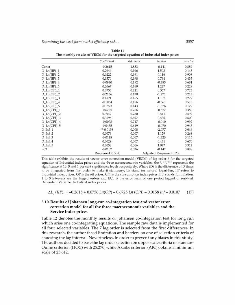
�Ln (IIP)
1 = –0.2615 + 0.0756 Ln(OP) – 0.6725 Ln (CPI) – 0.0158 Inf – 0.0107 (17)
5.10. Results of Johansen long-run co-integration test and vector errorcorrection model for all the three macroeconomic variables and theService Index prices
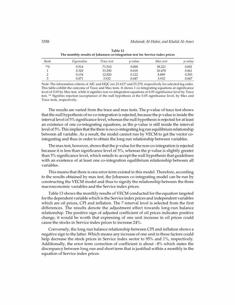
Table 12 denotes the monthly results of Johansen co-integration test for long runwhich arise one co-integrating equations. The sample raw data is implemented forall four selected variables. The 7 lag order is selected from the first differences. Inthis research, the author faced limitation and barriers on one of selection criteria ofchoosing the lag interval. Nevertheless, in order to prevent any biases in this study.The authors decided to base the lag order selection on upper scale criteria of Hannan-Quinn criterion (HQC) with 25.270, while Akaike criterion (AIC) obtains a minimumscale of 23.612.
Table 11The monthly results of VECM for the targeted equation of Industrial index prices
Coefficient std. error t-ratio p-value
Const -0.2615 1.853 -0.141 0.889D_Ln(IIP)_1 0.2944 0.196 1.503 0.143D_Ln(IIP)_2 0.0222 0.191 0.116 0.908D_Ln(IIP)_3 0.1570 0.198 0.794 0.433D_Ln(IIP)_4 -0.0930 0.192 -0.485 0.631D_Ln(IIP)_5 0.2067 0.169 1.227 0.229D_Ln(OP)_1 0.0756 0.211 0.357 0.723D_Ln(OP)_2 -0.2166 0.170 -1.271 0.213D_Ln(OP)_3 0.1821 0.165 1.107 0.277D_Ln(OP)_4 -0.1034 0.156 -0.661 0.513D_Ln(OP)_5 -0.1973 0.143 -1.376 0.179D_Ln(CPI)_1 -0.6725 0.766 -0.877 0.387D_Ln(CPI)_2 0.3947 0.730 0.541 0.592D_Ln(CPI)_3 0.3695 0.697 0.530 0.600D_Ln(CPI)_4 -0.0078 0.747 -0.010 0.992D_Ln(CPI)_5 -0.0455 0.649 -0.070 0.945D_Inf_1 **-0.0158 0.008 -2.077 0.046D_Inf_2 0.0079 0.007 1.129 0.268D_Inf_3 -0.0118 0.007 -1.623 0.115D_Inf_4 0.0029 0.007 0.431 0.670D_Inf_5 0.0058 0.006 1.027 0.312EC1 -0.0107 0.076 -0.142 0.888
R-squared: 0.538 Adjusted R-squared 0.235
This table exhibits the results of vector error correction model (VECM) of lag order 6 for the targetedequation of Industrial index prices and the three macroeconomic variables, the *, **, *** represents thesignificance at 10, 5 and 1 per cent significance levels respectively. Where (D) is the difference of D timesto be integrated from first order to make it stationary, Ln stand for natural logarithm, IIP refers toIndustrial index prices, OP is the oil prices, CPI is the consumption index prices, Inf. stands for inflation,1 to 5 intervals are the lagged orders and EC1 is the error term of one period lagged of residual.Dependent Variable: Industrial index prices
3358 Mubarak Al-Habsi, and Khalid Al-Amri
The results are varied from the trace and max tests. The p-value of trace test showsthat the null hypothesis of no co-integration is rejected, because the p-value is inside theinterval level of 5% significance level, whereas the null hypothesis is rejected for at leastan existence of one co-integrating equations, as the p-value is still inside the intervallevel of 5%. This implies that the there is no co-integrating log run equilibrium relationshipbetween all variable. As a result, the model cannot run by VECM to get the vector co-integrating and thus in order to obtain the long run relationship between variables.
The max test, however, shows that the p-value for the non-co-integration is rejectedbecause it is less than significance level of 5%, whereas the p-value is slightly greaterthan 5% significance level, which entails to accept the null hypothesis that guidelineswith an existence of at least one co-integration equilibrium relationship between allvariables.
This means that there is one error term existed in this model. Therefore, accordingto the results obtained by max test, the Johansen co-integrating model can be run byconstructing the VECM model and thus to signify the relationship between the threemacroeconomic variables and the Service index prices.
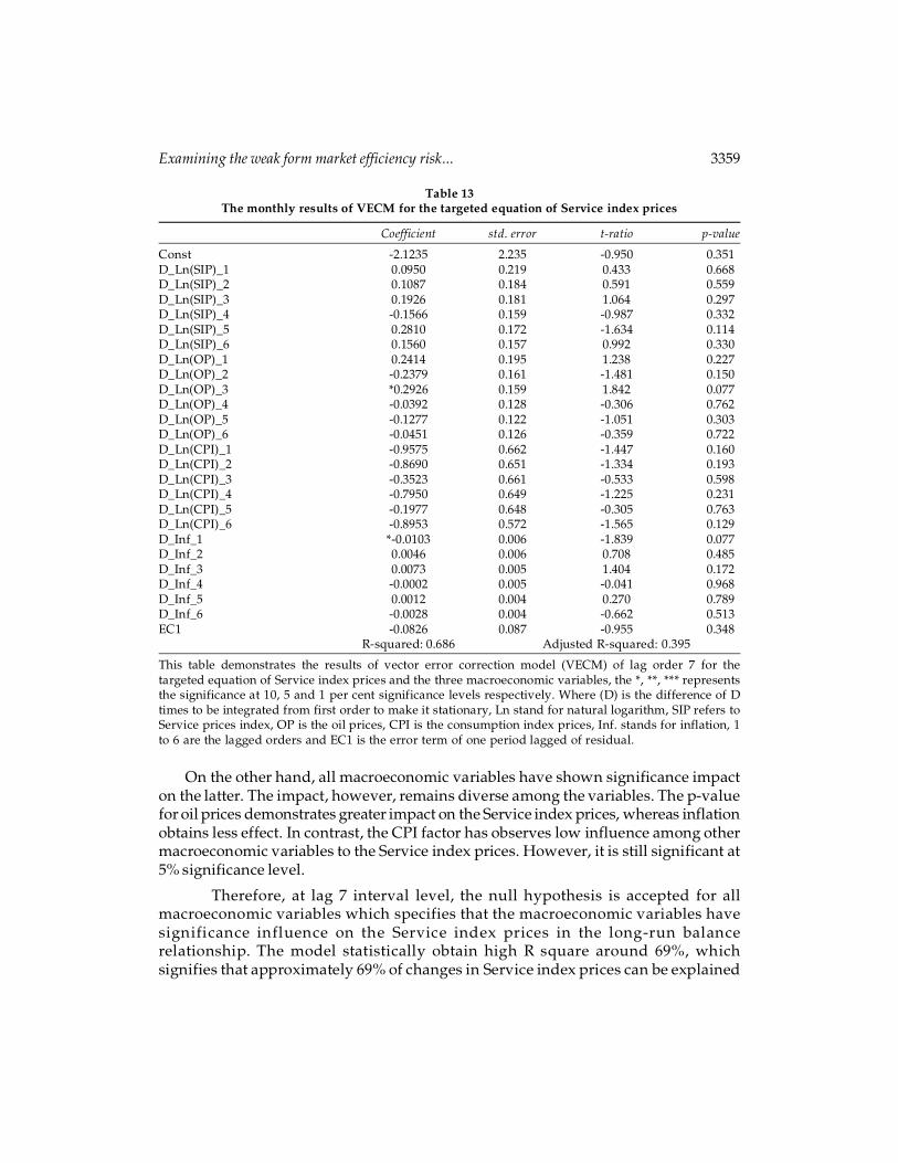
Table 13 shows the monthly results of VECM conducted for the equation targetedfor the dependent variable which is the Service index prices and independent variableswhich are oil prices, CPI and inflation. The 7 interval level is selected from the firstdifferences. The results denote the adjustment effect towards long-run balancerelationship. The positive sign of adjusted coefficient of oil prices indicates positivechange, it would be worth that expressing of one unit increase in oil prices couldcause the stocks in Service index prices to increase 24%.
Conversely, the long run balance relationship between CPI and inflation shows anegative sign to the latter. Which means any increase of one unit in these factors couldhelp decrease the stock prices in Service index sector to 95% and 1%, respectively.Additionally, the error term correction of coefficient is about –8% which states thediscrepancy between long run and short term that is justified within a monthly in theequation of Service index prices.
Table 12The monthly results of Johansen co-integration test for Service index prices
Rank Eigenvalue Trace test p-value Max test p-value
**0 0.514 71.510 0.000 38.221 0.0011 0.320 33.290 0.018 20.470 0.0612 0.154 12.820 0.122 8.889 0.3033 0.071 3.932 0.047 3.932 0.047
Note: The information criteria of AIC and HQC are 23.612* and 25.270, respectively for selected lag order.This table exhibit the outcome of Trace and Max tests. It shows 1 co-integrating equations at significancelevel of 0.05 by Max test, while it signifies non co-integration equations at 0.05 significance level by Tracetest. ** Signifies rejection (acceptance) of the null hypothesis at the 0.05 significance level, by Max andTrace tests, respectively.
Examining the weak form market efficiency risk... 3359
On the other hand, all macroeconomic variables have shown significance impacton the latter. The impact, however, remains diverse among the variables. The p-valuefor oil prices demonstrates greater impact on the Service index prices, whereas inflationobtains less effect. In contrast, the CPI factor has observes low influence among othermacroeconomic variables to the Service index prices. However, it is still significant at5% significance level.
Therefore, at lag 7 interval level, the null hypothesis is accepted for allmacroeconomic variables which specifies that the macroeconomic variables havesignificance influence on the Service index prices in the long-run balancerelationship. The model statistically obtain high R square around 69%, whichsignifies that approximately 69% of changes in Service index prices can be explained
Table 13The monthly results of VECM for the targeted equation of Service index prices
Coefficient std. error t-ratio p-value
Const -2.1235 2.235 -0.950 0.351D_Ln(SIP)_1 0.0950 0.219 0.433 0.668D_Ln(SIP)_2 0.1087 0.184 0.591 0.559D_Ln(SIP)_3 0.1926 0.181 1.064 0.297D_Ln(SIP)_4 -0.1566 0.159 -0.987 0.332D_Ln(SIP)_5 0.2810 0.172 -1.634 0.114D_Ln(SIP)_6 0.1560 0.157 0.992 0.330D_Ln(OP)_1 0.2414 0.195 1.238 0.227D_Ln(OP)_2 -0.2379 0.161 -1.481 0.150D_Ln(OP)_3 *0.2926 0.159 1.842 0.077D_Ln(OP)_4 -0.0392 0.128 -0.306 0.762D_Ln(OP)_5 -0.1277 0.122 -1.051 0.303D_Ln(OP)_6 -0.0451 0.126 -0.359 0.722D_Ln(CPI)_1 -0.9575 0.662 -1.447 0.160D_Ln(CPI)_2 -0.8690 0.651 -1.334 0.193D_Ln(CPI)_3 -0.3523 0.661 -0.533 0.598D_Ln(CPI)_4 -0.7950 0.649 -1.225 0.231D_Ln(CPI)_5 -0.1977 0.648 -0.305 0.763D_Ln(CPI)_6 -0.8953 0.572 -1.565 0.129D_Inf_1 *-0.0103 0.006 -1.839 0.077D_Inf_2 0.0046 0.006 0.708 0.485D_Inf_3 0.0073 0.005 1.404 0.172D_Inf_4 -0.0002 0.005 -0.041 0.968D_Inf_5 0.0012 0.004 0.270 0.789D_Inf_6 -0.0028 0.004 -0.662 0.513EC1 -0.0826 0.087 -0.955 0.348
R-squared: 0.686 Adjusted R-squared: 0.395
This table demonstrates the results of vector error correction model (VECM) of lag order 7 for thetargeted equation of Service index prices and the three macroeconomic variables, the *, **, *** representsthe significance at 10, 5 and 1 per cent significance levels respectively. Where (D) is the difference of Dtimes to be integrated from first order to make it stationary, Ln stand for natural logarithm, SIP refers toService prices index, OP is the oil prices, CPI is the consumption index prices, Inf. stands for inflation, 1to 6 are the lagged orders and EC1 is the error term of one period lagged of residual.
3360 Mubarak Al-Habsi, and Khalid Al-Amri
by the variability in macroeconomic variables. The adjusted R square is about 40%.Thus, the former and the latter measures suggest that R square rate is a good fit tofill the desirable of this model. As a result, the estimated co-integrating vectorslong term stable relationship of targeted model for Service index prices is appliedas following:
�Ln (SIP)
1 = –2.1235 + 0.2414 Ln(OP) – 0.9575 Ln (CPI) – 0.0103 Inf – 0.0826 (18)
6. CONCLUSION
This research ultimately considers and examines the ‘random walk’ theory andinvestigates the ‘weak form’ market efficient hypothesis of the Financial, Industrialand Service indices returns which are listed in the MSM30 index, over the monthlydata period from January 2014 to December 2014.
Tests are conducted to measure the ‘weak form’ market efficiency of these indices,and of these, there are serial correlational variants and variance ratio tests.Consequently, both tests are parametric, which is the most appropriate method fortesting normal distributed data. This area however, could be one of the limitations ofthe study, as other studies have used non-parametric tests in order to examine the‘weak form’ market efficiency.
Overall results of this study exhibit a clear reference of co-integrating relationshipsamong the variables. The results infer that indices prices are predictable based onhistorical information and other macroeconomic factors. Therefore, based on suchinference, investors do and will have a chance to outperform the stock indices andthus gain profit above market average through use of information regardingmacroeconomic variables in order to improve the prediction of the indices prices.Concluding thus is the inherent finding sought for, that the stock indices of Financial,Industrial and Services listed in MSM30 are inefficient in the ‘weak form’ of marketefficiency.
NOTES
1. The Muscat Securities Market (MSM) was founded in 1988. It lists over 152 companiescoming from Financial, Industrial and Service indices sectors. The market capitalizationposted its highest record in 2014, reaching OMR 14.560 billion over OMR 14.160 billion in2013 (Muscat Securities Market, 2015).
2. Investment decisions are aided thus: attempts to find mispriced assets have no benefit inan efficient market. In the efficient market investors may decide to invest considerably inselecting passive management in one of the sector, over another. Alternatively, if themarket is inefficient in a particular sector, it is an opportunity for the rational investor touse common analysis tools to outperform the market in order to achieve abnormal returns.In the inefficient market greater funds invested in active management of a particularsector which appears to be inefficient in EMH provides the opportunity to enhance returnsadjusted with risk, by recognizing the misprices in securities, and thus short selling theovervalued securities and buying the undervalued securities.
Examining the weak form market efficiency risk... 3361
3. The variance ratio and run tests methodology was developed by Beveridge and Nelson(1981).
4. The demonstration was rendered using multivariate vector auto regression, Johansen-Jueslius co-integration, Phillips-Perron and Kwiatkowski and Philips unit root tests,onmonthly data collected from January 1996 to December 2012.
5. This methodology was founded by Johansen and Juselius (1990).
6. Gujarati (2012) has defined time series as a set of data observations collected in differenttime intervals, every ten and five years, such as annually, monthly, weekly and daily.
7. The essential development of Q-Statistics was originated by Box and Pierce (1970).
8. The term (VECM) model term was first named by Sargan (1964) and later simplified byEngle and Granger (1987).
References
Abraham, A., Seyyed, F. J., and Alsakran, S. A., (2002), Testing the Random Walk Behavior andEfficiency of the Gulf Stock Markets. The Financial Review 37 (3), 469-480.
Akerl0f, G., (1970), The Market for “Lemons”: Quality Uncertainty and the MarketMechanism. The Quarterly Journal of Economics, 84 (3), 488-500.
Alexander, G. J. and Bailey, J. V., (1995). Investments. Prentice Hall,
Al-Jafari, M. K., (2012), An Empirical Investigation of the Day-of-the-Week Effect on StockReturns and Volatility: Evidence from Muscat Securities Market. International Journal ofEconomics and Finance 4 (7), 141.
Al-Raisi, A. H., Pattanaik, S., and al-Markazî al-»Umânî, B., (2006), MSM and the EfficientMarket Hypothesis: An Empirical Assessment. Central Bank of Oman, Economic Researchand Statistics Department,
Bachelier, L., (1900), Théorie De La Spéculation. Gauthier-Villars,
Bashir, T., Ilyas, M., and Furrukh, A., (2011), Testing the Weak-Form Efficiency of PakistaniStock Markets-an Empirical Study in Banking Sector. European Journal of Economics,Finance and Administrative Sciences 31, 160-175.
Bernard, C., and Boyle, P., (2009), Mr. Madhoff’s Amazing Returns: An Analysis of the Split-Strike Conversion Strategy. Journal of Derivatives 17 (1) 1-30
Beveridge, S. and Nelson, C. R., (1981), A New Approach to Decomposition of Economic TimeSeries into Permanent and Transitory Components with Particular Attention toMeasurement of the ‘business Cycle’. Journal of Monetary Economics 7 (2), 151-174.
Bloomberg, (2015), Bloomberg Business, [Online]. Accessed 21 May 2015. Available at: http://www.bloomberg.com/quote/CL1:COM
Bloomberg, (2015), Bloomberg Business, [Online]. Accessed 21 June 2015. Available at: http://www.bloomberg.com/news/articles/2015-06-08/china-stock-index-futures-swing-after-shanghai-gauge-tops-5-000
Box, G. E. and Pierce, D. A., (1970), Distribution of Residual Autocorrelations inAutoregressive-Integrated Moving Average Time Series Models. Journal of the AmericanStatistical Association 65 (332), 1509-1526.
Buguk, C. and Brorsen, B. W., (2003), Testing Weak-Form Market Efficiency: Evidence fromthe Istanbul Stock Exchange. International Review of Financial Analysis 12 (5), 579-590.

3362 Mubarak Al-Habsi, and Khalid Al-Amri
Butler, K. and Malaikah, S. J., (1992), Efficiency and Inefficiency in thinly traded stock markets:Kuwait and Saudi Arabia. Journal of Banking and Finance 16, 197-210.
Capital Market Authority., (2015), [Online]. Accessed 21 May 2015. Available at: http://www.cma.gov.om/Home/DecisionsCirculars
Chen, N., Roll, R., and Ross, S. A., (1986), Economic Forces and the Stock Market. Journal ofBusiness, 383-403.
Chepkoech Kemei, J., and Kenyatta, J., (2014), The Effect of Information Asymmetry in thePerformance of the Banking Industry: A Case Study of Banks in Mombassa County.International Journal of Educational Research 2 (2) 1-6.
Cheung, K. and Andrew Coutts, J., (2001), A Note on Weak Form Market Efficiency in SecurityPrices: Evidence from the Hong Kong Stock Exchange. Applied Economics Letters 8 (6),407-410.
Cheung, Y. and Ng, L. K., (1998), International Evidence on the Stock Market and AggregateEconomic Activity. Journal of Empirical Finance 5 (3), 281-296.
Cong, R., Wei, Y., Jiao, J., and Fan, Y., (2008), Relationships between Oil Price Shocks and StockMarket: An Empirical Analysis from China. Energy Policy 36 (9), 3544-3553.
Dockery, E. and Vergari, F., (1997), Testing the Random Walk Hypothesis: Evidence for theBudapest Stock Exchange. Applied Economics Letters 4 (10), 627-629.
Dyckman, T. and Morse, D., (1986), Efficient Capital Markets: A Critical Analysis. New Jersey,Prince-Hall, Englewood Cliffs.
Elango, D. and Hussein, M. I., (2008), An Empirical Analysis on the Weak-Form Efficiency ofthe GCC Markets Applying Selected Statistical Tests. International Review of BusinessResearch Papers 4 (1)
Engle, R. F. and Granger, C. W., (1987), Co-Integration and Error Correction: Representation,Estimation, and Testing. Econometrica: Journal of the Econometric Society, 251-276.
Fama, E. F. and French, K. R., (1998), Value Versus Growth: The International Evidence.Journal of Finance, 1975-1999.
Fama, E. F., (1991), Efficient Capital Markets: II. The Journal of Finance 46 (5), 1575-1617.Fama, E. F. and French, K. R., (1988), Permanent and Temporary Components of Stock Prices.
The Journal of Political Economy, 246-273.Fama, E. F., (1970), Efficient Capital Markets: A Review of Theory and Empirical Work. The
Journal of Finance 25 (2), 383-417.Fama, E. F. and Blume, M. E., (1966), Filter Rules and Stock-Market Trading. Journal of
Business, 226-241.Fama, E. F., (1965), The Behavior of Stock-Market Prices. Journal of Business, 34-105.Findlay, M. and Williams, E., (2000), A Fresh Look at the Efficient Market Hypothesis: How the
Intellectual History of Finance Encouraged a Real “Fraud-on-the-Market”. Journal of PostKeynesian Economics, 181-199.
Gay Jr, R. D., (2008), Effect of Macroeconomic Variables on Stock Market Returns for FourEmerging Economies: Brazil. Russia, India, and China Retrieved in International Financeand Economic Journal
Gujarati, D., (2014), Econometrics by Example. Palgrave Macmillan
Examining the weak form market efficiency risk... 3363
Gujarati, D. N., (2012), Basic Econometrics. Tata McGraw-Hill EducationHammoudeh, S. and Li, H., (2008), Sudden Changes in Volatility in Emerging Markets: The
Case of Gulf Arab Stock Markets. International Review of Financial Analysis 17 (1),47-63.
Hammoudeh, S., Dibooglu, S., and Aleisa, E., (2004), Relationships among US Oil Prices andOil Industry Equity Indices. International Review of Economics & Finance 13 (4), 427-453.
Healy, P., and Palepu, K., (2001), Information asymmetry, corporate disclosure, and the capitalmarkets: A review of the empirical disclosure literature. Journal of Accounting andEconomics 31, 405-440.
Huang, R. D., Masulis, R. W., and Stoll, H. R., (1996), Energy Shocks and Financial Markets.Journal of Futures Markets 16 (1), 1-27.
Hurt, C., (2010), Evil Has a New Name (and a New Narrative): Bernard Madhoff. MichiganState Law Review 10 (7) 947-973
Jawad, M. H., (2011), Testing the Muscat Securities Market for Weak-Form Efficiency. Availableat SSRN 1859332
Johansen, S. and Juselius, K., (1990), Maximum Likelihood Estimation and Inference onCointegration with Applications to the Demand for Money. Oxford Bulletin of Economicsand Statistics 52 (2), 169-210.
Johansen, S., (1988), Statistical Analysis of Cointegration Vectors. Journal of EconomicDynamics and Control 12 (2), 231-254.
Jones, C. M. and Kaul, G., (1996), Oil and the Stock Markets. The Journal of Finance 51 (2),463-491.
Jones, C. P., (2007), Investments: Analysis and Management. John Wiley & SonsKharusi, S. A. and Weagley, R. O., (2014), Weak Form Market Efficiency during the 2008
Financial Crisis: Evidence from the Muscat Securities Market. The International Journal ofBusiness and Finance Research 8 (4), 27-42.
Kilian, L. and Park, C., (2009), The Impact of Oil Price Shocks on the Us Stock Market.International Economic Review 50 (4), 1267-1287.
Kling, J. L., (1985), Oil Price Shocks and Stock Market Behavior. The Journal of PortfolioManagement 12 (1), 34-39.
Kreps, D., (1990), A course in microeconomic theory. Princeton University Press, Princeton,NJ. 1-864
Langevoort, D, (2002), Taming the Animal Spirits of the Stock Markets: A BehaviouralApproach to Securities Regulation. Northwestern University Law Review 97 (1) 135-158
Lee, U., (1992), Do Stock Prices Follow Random Walk?: Some International Evidence.International Review of Economics & Finance 1 (4), 315-327.
Ljung, G. M. and Box, G. E., (1978), On a Measure of Lack of Fit in Time Series Models.Biometrika 65 (2), 297-303.
Lo, A. W. and MacKinlay, A. C., (1988), Stock Market Prices do Not Follow Random Walks:Evidence from a Simple Specification Test. Review of Financial Studies 1 (1), 41-66.
Malkiel, B. G., (1999), A Random Walk Down Wall Street: Including a Life-Cycle Guide toPersonal Investing. WW Norton & Company
3364 Mubarak Al-Habsi, and Khalid Al-Amri
Maysami, R. C., Howe, L. C., and Hamzah, M. A., (2004), Relationship between MacroeconomicVariables and Stock Market Indices: Cointegration Evidence from Stock Exchange ofSingapore’s all-S Sector Indices. Journal Pengurusan 24 (1), 47-77.
Miller, M. H., Muthuswamy, J., and Whaley, R. E., (1994), Mean Reversion of Standard &Poor’s 500 Index Basis Changes: Arbitrage induced Or Statistical Illusion?. The Journal ofFinance 49 (2), 479-513.
Mukherjee, T. K. and Naka, A., (1995), Dynamic Relations between Macroeconomic Variablesand the Japanese Stock Market: An Application of a Vector Error Correction Model.Journal of Financial Research 18 (2), 223-237.
Muscat Securities Market., (2015), Publications- Yearly, [online]. Accessed 21 May 2015.Available at: https://www.msm.gov.om/
Muslumov, A., Aras, G., and Kurtulus, B., (2003), Evolving Market Efficiency in Istanbul StockExchange. Istanbul Technical University Selected Articles, 271-291.
National Center for Statistics & Information, (2015), Library Content Details, [online].Accessed 21 May 2015. Available at: http://www.ncsi.gov.om/Elibrary/Pages/LibraryContent Details. aspx?
Nishat, M., Shaheen, R., and Hijazi, S. T., (2004), Macroeconomic Factors and the PakistaniEquity Market [with Comments]. The Pakistan Development Review, 619-637.
Okpara, G. C., (2010), Stock Market Prices and the Random Walk Hypothesis: FurtherEvidence from Nigeria. Journal of Economics and International Finance 2 (3), 49-57.
Park, J. and Ratti, R. A., (2008), Oil Price Shocks and Stock Markets in the US and 13 EuropeanCountries. Energy Economics 30 (5), 2587-2608.
Penman, S. H., (1982), ‘Insider Trading and the Dissemination of Firms’ Forecast Information.Journal of Business, 479-503.
Rahman, M. L. and Uddin, J., (2009), Dynamic Relationship between Stock Prices andExchange Rates: Evidence from Three South Asian Countries. International BusinessResearch 2 (2), p. 167.
Redhead, K., (2008), Personal Finance and Investments: A Behavioural Finance Perspective.Routledge
Samuels, J., Yacout, N., and Samuels, I., (1981), Stock Exchanges in Developing countries/laBourse Des ValeursDans Les Pays EnVoie De Developpement. Savings and Development,217-232.
Sargan, J. D., (1964), Wages and Prices in the United Kingdom: A Study in EconometricMethodology. Econometric Analysis for National Economic Planning 16, 25-54.
Sedik, T. S. and Williams, M. O., (2011), Global and Regional Spillovers to GCC EquityMarkets. International Monetary Fund
Shaker, A. T. M., (2013), Testing the Weak-Form Efficiency of the Finnish and Swedish StockMarkets. European Journal of Business and Social Sciences 2 (9), 176-185.
Sharma, J. and Kennedy, R. E., (1977), A Comparative Analysis of Stock Price Behavior on theBombay, London, and New York Stock Exchanges. Journal of Financial and QuantitativeAnalysis 12 (03), 391-413.
Smith, G., (2007), Random Walks in Middle Eastern Stock Markets. Applied FinancialEconomics 17 (7), 587-596.
Examining the weak form market efficiency risk... 3365
Smith, G. and Ryoo, H., (2003), Variance Ratio Tests of the Random Walk Hypothesis forEuropean Emerging Stock Markets. The European Journal of Finance 9 (3), 290-300.
Solnik, B. H., (1973), Note on the Validity of the Random Walk for European Stock Prices.Journal of Finance, 1151-1159.
Suleman, M. T., Hamid, K., Ali Shah, S. Z., Akkash, I., and Shahid, R., (2010), Testing the WeakForm of Efficient Market Hypothesis: Empirical Evidence from Asia-Pacific Markets.International Research Journal of Finance and Economics (58), 121.
Summers, L. H., (1986), Does the Stock Market Rationally Reflect Fundamental Values?. TheJournal of Finance 41 (3), 591-601.
Tasker, S., (1998), Bridging the Information Gap: Quarterly Conference calls as a Medium forVoluntary Disclosure. Review of Accounting Studies, 3.
Urrutia, J. L., (1995), Tests of Random Walk and Market Efficiency for Latin AmericanEmerging Equity Markets. Journal of Financial Research 18 (3), 299-309.
Worthington, A. C. and Higgs, H., (2005), Weak-Form Market Efficiency in Asian Emergingand Developed Equity Markets: Comparative Tests of Random Walk Behaviour.
Yahyazadehfar, M. and Babaie, A., (2012), Macroeconomic Variables and Stock Price: NewEvidence from Iran. Middle-East Journal of Scientific Research 11 (4), 408-415.
Zychowicz, E. J., Binbasioglu, M., and Kazancioglu, N., (1995), The Behavior of Prices on theIstanbul Stock Exchange. Journal of International Financial Markets Institutions andMoney 5, 61-71.