ARCHIVES OF ACOUSTICS DOI: 10.2478/v10168-011-0051-7

36, 4, 761–775 (2011)

Examination of the Effect of a Sound Source Locationon the Steady-State Response of a Two-Room

Coupled System

Mirosław MEISSNERInstitute of Fundamental Technological ResearchPolish Academy of SciencesPawińskiego 5B, 02-106 Warszawa, Polande-mail: mmeissn@ippt.gov.pl

(received June 17, 2011; accepted August 8, 2011 )

In this paper, the computer modelling application based on the modal expansionmethod is developed to study the influence of a sound source location on a steady-state response of coupled rooms. In the research, an eigenvalue problem is solvednumerically for a room system consisting of two rectangular spaces connected to oneanother. A numerical procedure enables the computation of shape and frequency ofeigenmodes, and allows one to predict the potential and kinetic energy densities in asteady-state. In the first stage, a frequency room response for several source positionsis investigated, demonstrating large deformations of this response for strong andweak modal excitations. Next, a particular attention is given to studying how thechanges in a source position influence the room response when a source frequencyis tuned to a resonant frequency of a strongly localized mode.

Keywords: coupled room system, steady-state room response, potential and kineticenergy densities, localization of modes.

1. Introduction

Theoretical and numerical predictions of the sound field in concert halls, the-atres and sacral objects have recently attracted considerable attention withinthe field of architectural acoustics (Gołaś, Suder–Dębska, 2009; Kamisińskiet al., 2009; Kosała, 2009), since this interest is connected with a growing de-mand for the acoustical comfort in public spaces. The acoustic behaviour ofcoupled rooms has also been studied in the context of the architectural acoustics(Ermann, 2005; Bradley, Wang, 2010) because coupled-volume systems, com-posed of two or more spaces that are connected through acoustically transparentopenings, can be found in various buildings or constructions. The orchestra pit

762 M. Meissner

and balconies in opera houses or theatres coupled to the main floor as well aschurches with several naves and chapels are typical examples of architecturalobjects with a structure of coupled rooms (Martellotta, 2009). In order toobtain a better understanding and control of the acoustics in such room systems,it is vital to have an efficient theoretical or computational method for predictinga structure of sound field in coupled rooms. Nowadays, many numerical methodscan be used to estimate the sound field in coupled rooms, like diffusion-equationmodels (Billon et al., 2006; Xiang et al., 2009), statistical-acoustic models(Summers et al., 2004), the geometrical acoustics (Summers et al., 2005; Puet al., 2011) and the modal expansion method (Meissner, 2007, 2008b, 2010),also known as the modal analysis. The geometrical acoustics applies at best torooms with dimensions large compared to the wavelength. Moreover, this methodneglects diffraction phenomena since a propagation in straight lines is its mainpostulate. A theory that fully represents the phenomenology of the sound field(but more difficult) is the modal analysis because it bases upon the wave acous-tics. The wave approach can be used in a low-frequency range, thus this theoryhas a practical application for rooms with dimensions comparable with the soundwavelength.In the low-frequency limit, the coupled-room systems exhibit some interest-

ing effects like: the mode degeneration due to modification of the coupling area,confinement of an acoustic energy in a part of room system, called the local-ization of modes, and a considerable difference between a rate of sound decayin early and late stages of the reverberant process, known as a double slopeddecay. These phenomena have been investigated by the author in recent papers(Meissner, 2008c, 2009a,b,c, 2011). The current work focuses on the examina-tion of an effect of a sound source location on a steady-state response of coupledrooms. The research explores the geometry that often occurs in the reality whentwo rectangular subrooms with the same heights are connected to one another.A room response is described theoretically by means of a modal expansion ofthe sound field for a weakly damped room system. Eigenfunctions, resonant fre-quencies and modal damping coefficients were calculated numerically by the useof a computer implementation that exploits the forced oscillator method.

2. Room acoustics in low-frequency range

In the low-frequency range, the sound pressure field inside an air-filled enclo-sure is determined via a solution of a three-dimensional wave equation with speci-fied initial and boundary conditions. In this approach, the acoustic room responseis found as a superposition of individual responses of normal acoustic modes gen-erated inside the room by a harmonic sound source (Kuttruff, 1973). Acousticmodes are inherent properties of the enclosure, and are determined by a roomgeometry and impedance conditions at the room walls. Each mode is defined by

Examination of the Effect of a Sound Source Location. . . 763

the natural (resonant or modal) frequency ωn, the modal damping coefficient rnand the mode shape specified by the eigenfunction Φn(r), where r = (x, y, z)determines the position of the observation point and n = 0, 1, 2, . . . , N . The nat-ural number N determines the amount of modes, that should be included in theroom response. It depends on the total room absorption A because the range ofmodal frequencies is bounded from above by the frequency (Schroeder, 1996)

fs = c√

6/A, (1)

where c is the sound speed. Below fs the modal density is low and particu-lar modes can be decomposed from the room response. Thus, in multi-moderesonance systems the frequency fs marks the transition from individual, well-separated resonances to many overlapping modes. The functions Φn are mutuallycoupled through the impedance condition on absorptive walls

∂p

∂n= − ρ

Z

∂p

∂t, (2)

where p(r, t) is the sound pressure, ρ is the air density, Z is the wall impedanceand ∂/∂n is the derivative taken in a direction normal to the surface of theroom walls. However, in the low-frequency limit typical materials covering roomwalls are characterized by a low absorption: ℜe(Z)/ρc ≫ 1, thus it is possibleto assume that the shapes of modes are well approximated by the uncoupledeigenfunctions Φn determined for hard room walls (Dowell et al., 1977).Taking all this into account and assuming that a source term in the wave

equation has the form −q(r) cos(ωt), where q(r) and ω are the volume sourcedistribution and the source frequency, the sound pressure in a steady-state canbe determined by (Meissner, 2008a)

p(r, t) =

N∑

n=0

[An cos(ωt) +Bn sin(ωt)]Φn(r), (3)

An =c2(ω2

n − ω2)Qn

(ω2n − ω2)2 + 4r2nω

2, Bn =

2c2ωrnQn

(ω2n − ω2)2 + 4r2nω

2, (4)

where Qn are factors describing the sound source strength

Qn =

∫

V

q(r)Φn(r)dv, (5)

where V is the room volume, and the modal damping coefficients rn are deter-mined by

rn =ρc2

2

∫

S

Φ2n

Zds, (6)

764 M. Meissner

where S is the surface of all the room walls. The functions Φn are mutuallyorthogonal and are normalized in the volume V by the relation

∫

V

ΦmΦn dv = δmn, (7)

where δmn = 1 for m = n and δmn = 0 for m 6= n. A zero-order mode is theso-called Helmholtz mode having the resonant frequency ω0 equal to zero and thefollowing normalized eigenfunction: Φ0 = 1/

√V , which corresponds to a trivial

solution of the eigenvalue equation

∇2Φn +(ωn

c

)2Φn = 0. (8)

In a steady-state, a sound source located in a room produces the acousticenergy field with a spatial density that depends on the room shape, the surfaceimpedance on the room walls and the sound source parameters. The potentialacoustic energy is stored in the form of pressure, while the kinetic one is mani-fested as a particle velocity. In terms of these quantities, the potential and kineticenergy densities are written as

wp(r) =1

2ρc2⟨p2⟩, wk(r) =

1

2ρ〈u · u〉, (9)

where 〈·〉 is the time-averaging, u is the particle velocity vector, and a dot denotesthe scalar product. After using Eqs. (3), (4) and the momentum equation

ρ∂u

∂t= −∇p, (10)

the potential energy density wp(r) can be expressed as

wp(r) =1

4ρc2

[N∑

n=0

AnΦn(r)

]2+

[N∑

n=0

BnΦn(r)

]2 (11)

and the kinetic energy density wk(r) as

wk(r) =1

4ρω2

(

N∑

n=0

An∂Φn

∂x

)2

+

(N∑

n=0

An∂Φn

∂y

)2

+

(N∑

n=0

An∂Φn

∂z

)2

+

(N∑

n=0

Bn∂Φn

∂x

)2

+

(N∑

n=0

Bn∂Φn

∂y

)2

+

(N∑

n=0

Bn∂Φn

∂z

)2 . (12)

These equations indicate that time-averaged energetic quantities of the acousticfield depend directly on the modal parameters: ωn, rn, Φn and the source fre-quency ω, and indirectly on the position and spatial distribution of the soundsource through the parameter Qn.

Examination of the Effect of a Sound Source Location. . . 765

When a room is excited by a point sound source with the power P , thesource function q(r) has the form of delta function i.e. q(r) = Qδ(r− r0), wherer0 = (x0, y0, z0) determines the position of source point and the parameter Q isgiven by (Kinsler, Frey, 1962)

Q =√

8πρcP . (13)In this case, the potential and kinetic energy densities are as follows:

wp(r) =Q2

4ρc2

[N∑

n=0

anΦn(r0)Φn(r)

]2+

[N∑

n=0

bnΦn(r0)Φn(r)

]2, (14)

wk(r) =Q2

4ρω2

[N∑

n=0

anΦn(r0)∂Φn

∂x

]2+

[N∑

n=0

anΦn(r0)∂Φn

∂y

]2

+

[N∑

n=0

anΦn(r0)∂Φn

∂z

]2+

[N∑

n=0

bnΦn(r0)∂Φn

∂x

]2

+

[N∑

n=0

bnΦn(r0)∂Φn

∂y

]2+

[N∑

n=0

bnΦn(r0)∂Φn

∂z

]2, (15)

where an = An/Qn and bn = Bn/Qn. Since the right-hand side of Eq. (14) isa symmetric function of the sound source and the observation points coordinates,in the case of the potential energy density the reciprocity principle is valid. Thismeans that when we put the source at r, we observe at point r0 the same potentialenergy density as we did before at r, when the source was located at r0. As itis evident from Eq. (15), the reciprocity principle is not satisfied for the kineticenergy density.

3. Computer simulation of steady-state room response

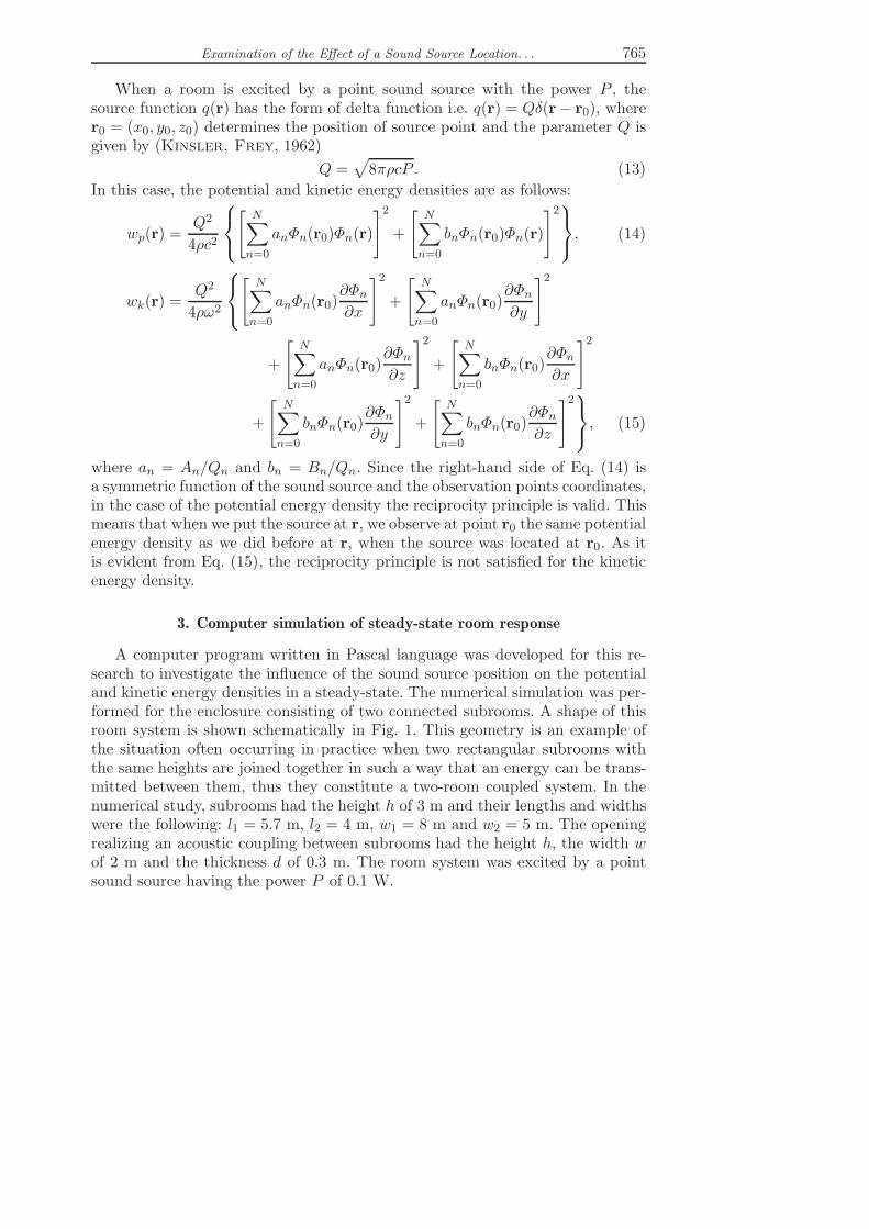
A computer program written in Pascal language was developed for this re-search to investigate the influence of the sound source position on the potentialand kinetic energy densities in a steady-state. The numerical simulation was per-formed for the enclosure consisting of two connected subrooms. A shape of thisroom system is shown schematically in Fig. 1. This geometry is an example ofthe situation often occurring in practice when two rectangular subrooms withthe same heights are joined together in such a way that an energy can be trans-mitted between them, thus they constitute a two-room coupled system. In thenumerical study, subrooms had the height h of 3 m and their lengths and widthswere the following: l1 = 5.7 m, l2 = 4 m, w1 = 8 m and w2 = 5 m. The openingrealizing an acoustic coupling between subrooms had the height h, the width wof 2 m and the thickness d of 0.3 m. The room system was excited by a pointsound source having the power P of 0.1 W.

766 M. Meissner

Fig. 1. Irregularly shaped enclosure consisting of two connected rectangular subroomsdenoted by A and B.

In the simulation it was assumed that the walls of the subrooms are coveredby an absorbing material providing a low sound damping, and the random-absorption coefficient α characterizes the damping properties of this material.For the sake of the model simplicity, the wall impedance corresponding to thisabsorption coefficient was purely real, i.e. the mass and stiffness of the absorbingmaterial were neglected. This is equivalent to the damping of a sound wave withno phase change upon reflection. In this case, for a given value of the coefficientα, the wall impedance on the subrooms’ walls was found from the equation(Kinsler, Frey, 1962)

α =8

ξ

[1 +

1

1 + ξ− 2

ξln(1 + ξ)

], (16)

where ξ = R/ρc is the impedance ratio and R is the wall resistance.In the case of an irregular room geometry, the first step towards determin-

ing the room response in a steady-state is a computation of the eigenfunctionsΦn, the resonant frequencies ωn and the modal damping coefficients rn. Sincea lightly damped room is considered, the functions Φn may be approximated byeigenfunctions computed for perfectly rigid room walls. Thus, the expression forΦn can be written as

Φn(r) =

Θk cos

(πkz

h

)Ψm(x, y)

√h

, (17)

where k = 0, 1, 2, . . . ,K and Θk = 1 for k = 0 and Θk =√2 for k > 0. The

eigenfunctions Ψm, m = 0, 1, 2, . . . ,M , are normalized over the room horizontalcross-section and Ψ0 = 1/

√Sc, where Sc = V/h is the surface of this cross-

section. The distributions of Ψm were found by means of a direct solution of the

Examination of the Effect of a Sound Source Location. . . 767

two-dimensional wave equation by a numerical procedure employing the forcedoscillator method. This method is based on the principle that the response ofa linear system to a harmonic excitation is large when the driving frequency isclose to the resonant frequency (Nakayama, Yakubo, 2001). Using Eq. (17) inEq. (8) it is easy to find that a formula for the resonant frequencies ωn is as follows

ωn =

√(πkc

h

)2

+ ω2m, (18)

where ωm are the resonant frequencies corresponding to Ψm. When the eigenfunc-tions Ψm were known, ωm were calculated from the eigenvalue equation, ∇2Ψm+(ωm/c)2Ψm = 0, multiplying it by Ψm, integrating and applying the orthogonalproperty. Next, using Eq. (6) the modal damping coefficients rn were computed.The computer simulation of a steady-state room response was performed for

the absorption coefficient α of 0.1. Since the total room absorption A is simplyequal to αS, where, as earlier, S denotes the surface of all the room walls, then,using Eq. (1), it is easy to calculate that the frequency fs, corresponding to thisvalue of α, is 165 Hz, approximately. Below this frequency 130 acoustic modeswere found. The distribution of the modulus of the eigenfunction Ψm for somemodes is plotted in Fig. 2. These graphs illustrate four fundamental shapes ofresonant modes. In the first case (Fig. 2a), the acoustic mode may be identifiedas a delocalized mode because its energy is reasonably uniformly distributed

Fig. 2. Modulus of the eigenfunction Ψm for the mode number m:a) 27, b) 34, c) 36, d) 45.

768 M. Meissner

inside the room. On the other hand, the next three modes are recognized aslocalized modes since their energy is concentrated in different parts of the roomsystem: the subroom A (Fig. 2b), the subroom B (Fig. 2c) and a portion of thesubroom A (Fig. 2d). Confinement of the acoustic energy in a restricted part ofrooms, known as the mode localization, is characteristic for systems of coupledrooms and enclosures with an irregular geometry (Meissner, 2005), because inrectangular rooms all eigenmodes are delocalized.When a lightly damped room is excited by the harmonic point source, a sound

signal received at the observation point is dominated by an individual responseof the normal acoustic mode whose modal frequency is very close to the sourcefrequency ω. Thus, if the source frequency varies, the acoustic signal perceivedat this point may change considerably because the response of a single modedepends on the value and slope of its eigenfunction at the source and observationpoints, as it results from Eqs. (14) and (15). This is clearly confirmed by the

Fig. 3. Frequency dependence of the potential energy density wp at the observation pointx = 3 m, y = 5 m, z = 1.8 m for the source positions (in meters): a) x0 = 2, y0 = 6, z0 = 1,

b) x0 = 2, y0 = 3, z0 = 1, c) x0 = 5, y0 = 3, z0 = 1, d) x0 = 8, y0 = 3, z0 = 1.

Examination of the Effect of a Sound Source Location. . . 769

simulation data depicted in Fig. 3 showing, for four different source positions, anevolution of the potential energy density wp with the source frequency f = ω/2π.As it may be seen, there is a substantial influence of the source position on thevalue of wp. However, more interesting from the practical point of view is thefinding that the frequency response of the room is highly deformed by modeswhich strongly respond to a sound excitation because it manifests itself as a high,narrow peak in the frequency dependence of wp.Now, if simulation results from Fig. 3b are shown in a logarithmic scale, one

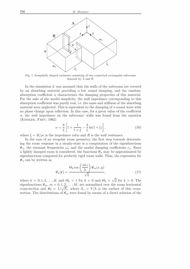
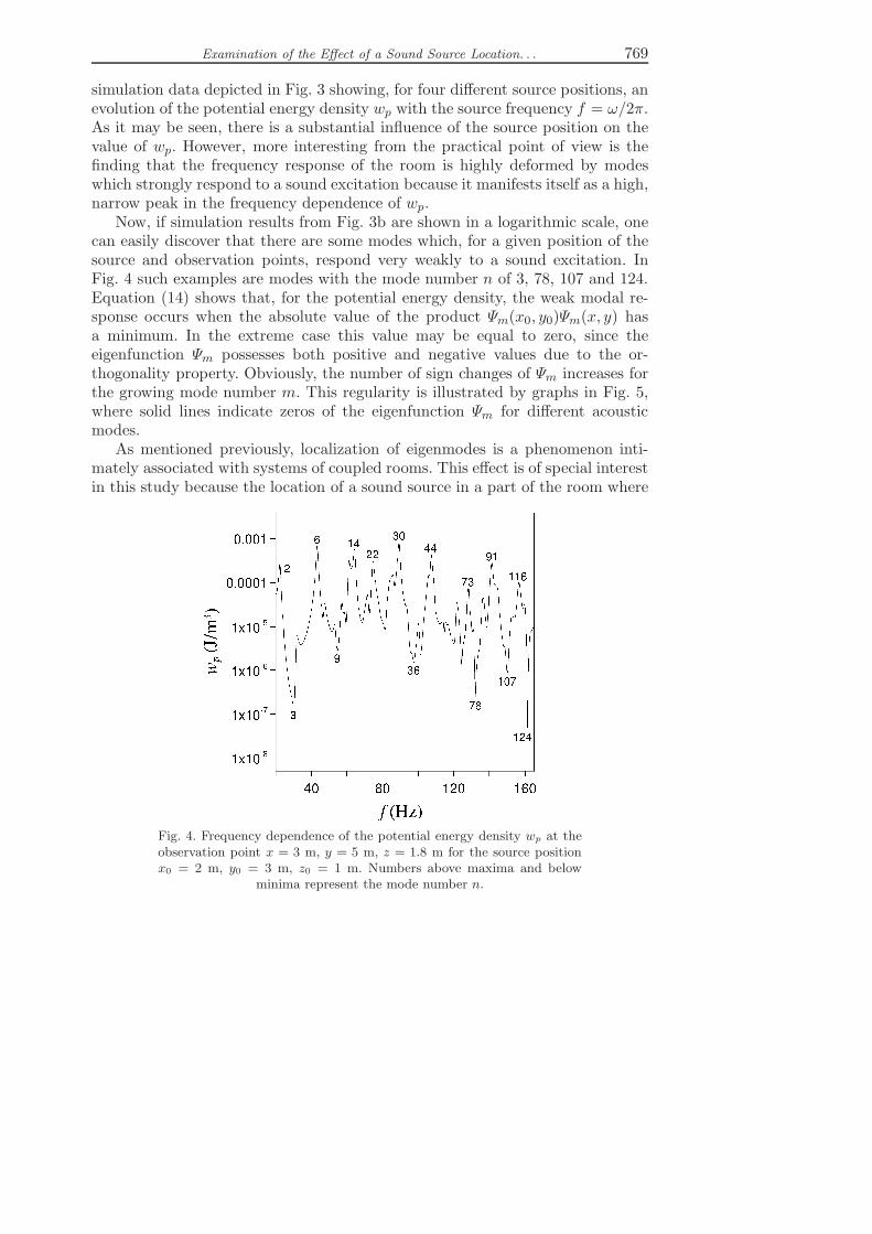
can easily discover that there are some modes which, for a given position of thesource and observation points, respond very weakly to a sound excitation. InFig. 4 such examples are modes with the mode number n of 3, 78, 107 and 124.Equation (14) shows that, for the potential energy density, the weak modal re-sponse occurs when the absolute value of the product Ψm(x0, y0)Ψm(x, y) hasa minimum. In the extreme case this value may be equal to zero, since theeigenfunction Ψm possesses both positive and negative values due to the or-thogonality property. Obviously, the number of sign changes of Ψm increases forthe growing mode number m. This regularity is illustrated by graphs in Fig. 5,where solid lines indicate zeros of the eigenfunction Ψm for different acousticmodes.As mentioned previously, localization of eigenmodes is a phenomenon inti-

mately associated with systems of coupled rooms. This effect is of special interestin this study because the location of a sound source in a part of the room where

Fig. 4. Frequency dependence of the potential energy density wp at theobservation point x = 3 m, y = 5 m, z = 1.8 m for the source positionx0 = 2 m, y0 = 3 m, z0 = 1 m. Numbers above maxima and below

minima represent the mode number n.

770 M. Meissner

Fig. 5. Lines indicating zeros of the eigenfunction Ψm for the mode number m:a) 10, b) 20, c) 35, d) 50.

the modal energy is very small may result in large decreases in the potential andkinetic energy densities. This problem will be analysed in detail for a mode withthe mode number n of 73, which was found to be localized in the subroom A.The modulus of the eigenfunction Ψm for this mode is depicted in Fig. 2b. Theresults of computer simulations of wp and wk in the observation plane, situatedat a constant height from the floor, are shown in Figs. 6 and 7. In the simulationit was assumed that a source frequency is tuned to the resonant frequency ofthe mode and there are two positions of the source: one in the subroom A andanother one in the subroom B. Figures 2b and 6a show that placing of the soundsource at an appropriate point of the subroom A results in a strong modal re-sponse because the distribution of the potential energy density wp in (x, y) planereproduces the square of the eigenfunction Ψm corresponding to the mode 73.On the other hand, the room response is very weak when the source is situatedin the subroom B where the energy of this mode is small (Fig. 6b). Moreover,the distribution of wp looks completely different from the previous case becausethe room response is now created by the surrounding modes. The kinetic energydensity wk, as seen in Fig. 7, is several dozen times smaller than the potentialone, and according to Eq. (15), in the case of strong room response, its distri-bution in (x, y) plane is proportional to (∂Ψm/∂x)2 + (∂Ψm/∂y)2, where Ψm isthe eigenfunction for the mode 73. This means that maxima of wp correspond to

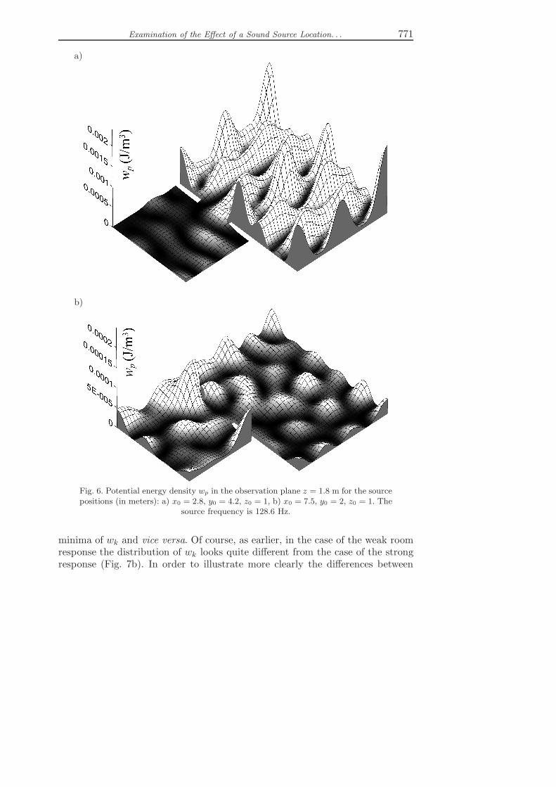
Examination of the Effect of a Sound Source Location. . . 771

a)

b)

Fig. 6. Potential energy density wp in the observation plane z = 1.8 m for the sourcepositions (in meters): a) x0 = 2.8, y0 = 4.2, z0 = 1, b) x0 = 7.5, y0 = 2, z0 = 1. The

source frequency is 128.6 Hz.

minima of wk and vice versa. Of course, as earlier, in the case of the weak roomresponse the distribution of wk looks quite different from the case of the strongresponse (Fig. 7b). In order to illustrate more clearly the differences between

772 M. Meissner

a)

b)

Fig. 7. Kinetic energy density wk in the observation plane z = 1.8 m for the sourcepositions (in meters): a) x0 = 2.8, y0 = 4.2, z0 = 1, b) x0 = 7.5, y0 = 2, z0 = 1. The

source frequency is 128.6 Hz.

the strong and weak room responses, in Fig. 8 the dependencies of wp and wk

on the coordinate y for a constant value of the coordinate x are shown. For thestrong response, the intense wavy changes in wp and wk are noted, because forthe mode considered acoustic resonance is excited between the walls separatedby the distance w1 (Fig. 1). The weak response also has a wave-like nature but its

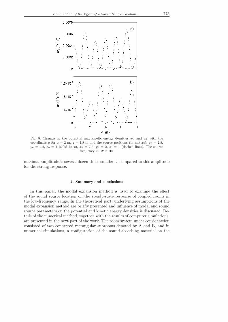
Examination of the Effect of a Sound Source Location. . . 773

Fig. 8. Changes in the potential and kinetic energy densities wp and wk with thecoordinate y for x = 2 m, z = 1.8 m and the source positions (in meters): x0 = 2.8,y0 = 4.2, z0 = 1 (solid lines), x0 = 7.5, y0 = 2, z0 = 1 (dashed lines). The source

frequency is 128.6 Hz.

maximal amplitude is several dozen times smaller as compared to this amplitudefor the strong response.

4. Summary and conclusions

In this paper, the modal expansion method is used to examine the effectof the sound source location on the steady-state response of coupled rooms inthe low-frequency range. In the theoretical part, underlying assumptions of themodal expansion method are briefly presented and influence of modal and soundsource parameters on the potential and kinetic energy densities is discussed. De-tails of the numerical method, together with the results of computer simulations,are presented in the next part of the work. The room system under considerationconsisted of two connected rectangular subrooms denoted by A and B, and innumerical simulations, a configuration of the sound-absorbing material on the

774 M. Meissner

room walls was assigned to the system. The simulation results have shown thatin the case of a harmonic excitation the sound signal received at the observationpoint is dominated by an individual response of the normal acoustic mode whosefrequency is close to the source frequency. Therefore, if the source frequencyvaries, the acoustic signal perceived at this point changes considerably becausethe response of a single mode depends on the value and slope of its eigenfunc-tion at the source and observation points. It was found that for different sourcepositions this results in large deformations of the frequency room response forstrong and weak modal excitations because they manifest themselves either ashigh peaks or as large drops in the response. The influence of the source positionon the room response is especially evident for localized modes. This problem wasexamined in detail for the mode strongly localized in the subroom A. Simulationsrevealed that when a source frequency is tuned to a resonant frequency of thismode placing of the point source inside the subroom A may result in the strongroom response, while location of the source inside the subroom B, where there isa small concentration of the modal energy, always leads to a very weak response.

References

1. Billon A., Valeau V., Sakout A., Picaut J. (2006), On the use of a diffusion model foracoustically coupled rooms, Journal of the Acoustical Society of America, 120, 2043–2054.

2. Bradley D.T., Wang L.M. (2010), Optimum absorption and aperture parameters for re-alistic coupled volume spaces determined from computational analysis and subjective testingresults, Journal of the Acoustical Society of America, 127, 223–232.

3. Dowell E.H., Gorman G.F., Smith D.A. (1977), Acoustoelasticity: general theory,acoustic natural modes and forced response to sinusoidal excitation, Journal of Sound andVibration, 52, 519–542.

4. Gołaś A., Suder–Dębska K. (2009), Analysis of Dome Home Hall theatre acoustic field,Archives of Acoustics, 34, 3, 273–293.

5. Ermann M. (2005), Coupled volumes: aperture size and the double-sloped decay of concerthalls, Building Acoustics, 12, 1–14.

6. Kamisiński T., Burkot M., Rubacha J., Brawata K. (2009), Study of the effect ofthe orchestra pit on the acoustics of the Kraków Opera Hall, Archives of Acoustics, 34, 4,481–490.

7. Kinsler L.E., Frey A.R. (1962), Fundamentals of acoustics, John Wiley & Sons, NewYork.

8. Kosała K. (2009), Calculation models for acoustic analysis of sacral objects, Archives ofAcoustics, 34, 1, 3–11.

9. Kuttruff H. (1973), Room acoustics, Applied Science Publishers, London.

10. Martellotta F. (2009), Identifying acoustical coupling by measurements and prediction-models for St. Peter’s Basilica in Rome, Journal of the Acoustical Society of America, 126,1175–1186.

Examination of the Effect of a Sound Source Location. . . 775

11. Meissner M. (2005), Influence of room geometry on low-frequency modal density, spatialdistribution of modes and their damping, Archives of Acoustics, 30, 4 (Supplement), 205–210.

12. Meissner M. (2007), Computational studies of steady-state sound field and reverberantsound decay in a system of two coupled rooms, Central European Journal of Physics, 5,293–312.

13. Meissner M. (2008a), Influence of wall absorption on low-frequency dependence of rever-beration time in room of irregular shape, Applied Acoustics, 69, 583–590.

14. Meissner M. (2008b), Acoustics of irregular rooms in buildings: low-frequency mathemat-ical modelling and numerical simulation, [in:] Renewable Energy, Innovative Technologiesand New Ideas, Chwieduk D., Domański R., Jaworski M. [Eds.], pp. 265–272, PublishingHouse of Warsaw University of Technology, Warsaw.

15. Meissner M. (2008c), Influence of absorbing material distribution on double slope sounddecay in L-shaped room, Archives of Acoustics, 33, 4 (Supplement), 159–164.

16. Meissner M. (2009a), Computer modelling of coupled spaces: variations of eigenmodesfrequency due to a change in coupling area, Archives of Acoustics, 34, 2, 157–168.

17. Meissner M. (2009b), Spectral characteristics and localization of modes in acousticallycoupled enclosures, Acta Acustica united with Acustica, 95, 300–305.

18. Meissner M. (2009c), Application of Hilbert transform-based methodology to computermodelling of reverberant sound decay in irregularly shaped rooms, Archives of Acoustics,34, 4, 491–505.

19. Meissner M. (2010), Simulation of acoustical properties of coupled rooms using numericaltechnique based on modal expansion, Acta Physica Polonica A, 118, 123–127.

20. Meissner M. (2011), Numerical modelling of coupled rooms: evaluation of decay times viamethod employing Hilbert transform, Acta Physica Polonica A, 119, 1031–1034.

21. Nakayama T., Yakubo K. (2001), The forced oscillator method: eigenvalue analysis andcomputing linear response functions, Physics Reports, 349, 239–299.

22. Pu H., Qiu X., Wang J. (2011), Different sound decay patterns and energy feedback incoupled volumes, Journal of the Acoustical Society of America, 129, 1972–1980.

23. Schroeder M. (1996), The “Schroeder frequency” revisited, Journal of the AcousticalSociety of America, 99, 3240–3241.

24. Summers J.E., Torres R.R., Shimizud Y. (2004), Statistical-acoustics models of energydecay in systems of coupled rooms and their relation to geometrical acoustics, Journal ofthe Acoustical Society of America, 116, 958–969.

25. Summers J.E., Torres R.R., Shimizud Y., Dalenback B.L. (2005), Adapting a ran-domized beam-axis-tracing algorithm to modeling of coupled rooms via late-part ray tracing,Journal of the Acoustical Society of America, 118, 1491–1502.

26. Xiang N., Jing Y., Bockman A.C. (2009), Investigation of acoustically coupled enclo-sures using a diffusion-equation model, Journal of the Acoustical Society of America, 126,1187–1198.