Examination of the difference between radiative and aerodynamic ...

'a n --- ~ , -

ELSEVIER

I

J

I

Examination of the Difference between Radiative and Aerodynamic Surface

' Temperatures over Sparsely , Vegetated 'Surfaces

%', ,

A. Chehbouni,* D. Lo Seen,'.$ E. G. Njoku,' and B. M. Monteny* I / - I' , .

A f m r - l q e r hydrologic model, coupled to a' vegetation growth model, has been used to investigate the differences between aerodynamic surface temperature and radiative surface temperature over sparsely vegetated surface. The rationale for the coupling of the two models was to assess the dependency of these differaxes on changing surfàce conditions (i.e., growing vegetation). A simulation was carried otct fw a 3 m n t h period corresponding to a typical growth seasonal cycle of an herbaceous canopy in the Sahel regwn of West Africa (Goutorbe et al., 1993). The results showed that the ratio of radiative-aerody- numic temperature difference to radiative-air temperature diffèreme was constant for a given day. However, the seasonal trend of this ratio was changing with respect to the leaf area index (LAI). A parameterization involving radiative surJace temperature, air temperature, and LAI was then developed to estimate aerodynamic-air temperature gradient, and thus sensible heat flux. This parameterization was validated wing data collected over herbaceous site during the Hapex-Sahel experiment. This approach was further advanced by wing a radiative transfer model in conjunction with the above models to simulate the temporal behavior of surface reflectances in the visible and the neur-infrared spectral bands. The result showed that sensible heat flux can be fairly accurately estimated b y combining remotely sensed surJace temperature, air temperature, and spectral vegetation

. .

* ORSTOM, Department Terre-Océan-Atmosphère, Montpel-

'Jet Propulsion Laboratory, California Institute of Technology,

*Present affiliation: CIRAD, Montpellier, France. Address correspondence to A. Chehbouni, Hydrology Lab., ORS-

Eleceived 1 March 1995; revised 18 January 1996.

lier, France

Pasadena, California, USA

TOM, 911 Av. Agropolis, BP 5045, 30042, Montpellier, France.

REMOTE SENS. ENVIRON. 58:177-186 (1996) @Elsevier Science Inc., 1996 655 Avenue of the Americas, New York, NY 10010 I

index. The result of this study m a y represent a great opportunity of using remotely sensed data to estimate spatiotemporal variabilities of surface fluxes in arid and semiarid regions.

:--- I.

W ' , i? "7

LNTRODUCTION z

O Elsevier Science Inc., 1996 8 .

T i

Thermal infrared remotely sensed surface temperatures are increasingly being used in simple, operational hydro- meteorological models to evaluate the spatial variation in the energy balance components over large ares (Jack- son, 1985). While this approach has been found to be successful over surfaces with near full canopy cover with unstressed transpiration, its performance has been questioned over sparsely vegetated surfaces.

From a theoretical vie^ point, sensible heat flux should be expressed in terms of aerodynamic surface temperature since it is aerodynamic temperature that

' determines the loss of sensible heat flux from a surface. Aerodynamic surface temperature was formally defined as the extrapolation of air temperature profile down to an effective height within the canopy at which the vegetation components of sensible and latent heat flux arise, say (d + Zh), 'where zh is the roughness length for heat and d is the zero-plane displacement height assumed to be the same for heat and for momentum (Kalma and Jupp, 1990). The formulation of sensible heat flux using this definition of aerodynamic surface temperature requires, however, an additional resistance to the classical log-profile aerodynamic resistance. This additional resistance, which is called the "excess" resistance, is meznt to take into account the fact that there is no thermal equivalent of bIuff body force. Therefore, the resistance for heat transfer is higher than the corre-

0034-4257 I96 I$15.00 PII SOO34-4257(96)00037-5

I

178 Chehbouni et al.

sponding resistance for momentum. The excess resistance has been formulated in terms of ln(z,,Izh) or its equivalent kB-l parameter (Chamberlain, 1968), where G is the roughness length for momentum transfer, wbi& is situated at a lower level than zh- Cr?~entSy reported values of kB-l range between 2 and 10 (Brut- seart, 1982). While the roughness length for momentum (zm) can be derived from the similarity theory or as a fraction of the canopy height, the estimation of the

‘ roughness length for heat ( zh ) is not trivial, especially over sparsely vegetated smfaces. The idea suggested by Montei& in 1963 (cited by Troufleau et al., 1996) was to. consider that the exchange of heat and moisture

;,between the surface and the atmosphere takes place at ‘an effective level located at the same height as the effective sink of momentum, that is, level d + zm, which corresponds to the level where the logarithmic profile takes its surface value. Then a new aerodynamic temperature was defined as the extrapolation of air temperature profile down to this level. It is confusing that no distinc- tion has been made in the literature between the two expressions of aerodynamic surface temperature. For consistent terminology, one may suggest that the temperature defined at level d + z h could be “convective” aerodynamic temperature and that defined at level d+z,,,, momentum aerodynamic temperature. In this study, however, we have solely addressed the case of momentum aerodynamic temperature, and have termed it aerodynamic temperature in the remaining part of the article.

Since aerodynamic temperature cannot be directly measured, it is often replaced by radiative temperature in the formulation of sensible heat flux. The problem is that the derivation of exchange coefficient &om Monin- Obukhov similarity theory does not apply when the surface radiative temperature is used instead of aerodynamic temperature ín the surface heat flux formulation (Sun and Mahrt, 1995). Under dense canopy, the W e r - ence between aerodynamic and radiative surface temperatures is very small, which leads to small errors in heat flux prediction. Over sparsely vegetated surfaces, however, the difference can exceed IOOC, as a result sensible heat flux can be largely overestimated.

Three different approaches for using remote sensing of surface temperature to estimate sensible heat flux over sparsely vegetated surfaces have been suggested in the literature. The first approach is to substitute radiative surface temperature for aerodynamic surface temperature and to add supplementary resistance to the aerodynamic resistance (see Lhomme et al., 1996). Kustas et al. (1989) suggested that this resistance can be formulated empirically as a function of wind speed and surface-air temperature gradient, that is, as

= uu (T, - T‘a), where u is the wind speed, Ta is air temperature, and the coefficient a is an empirical factor that was found to be 0.17 from observations of sparse

,

vegetation in California and 0.11 for data from Arizona (Kustas et al., 1989; Moran et al., 1994). It must be emphasized, however, that this resistance should not be called kB-‘; this may induce a confusion between

proach is to determine a new stability function or define a radiometric exchange coefficient (Sun and Mahrt, 1995) that allowed accurate predictions of heat flux when radiative surface temperature is used. The third approach consists of formulating a relationship between aerodynamic and radiative surface temperature (Brut- saert, 1982). This is a very difficult task since T,. is a function of radiative and kinetic temperature of the surface, sensor view angle, and surface morphology, while To is a mathematical construct that depends upon the surface radiative and kinetic temperature and on the thermodynamic properties of the air in contact with the surface (Hall et al., 1992).

In a similar vein, the objective of the present study were: 1) to examine the differences between radiative and aerodynamic temperatures for sparsely vegetated surfaces, and to determine whether a consistent relationship between aerodynamic-air temperature gradient and radiativeair temperatuie o& could be found, and 2) to investigate the possibility of thereby obtaining accurate estimates of sensible heat flux from ancillarymeteorolog- ical input and remotely sensed data in the visible, NIR, and thermal infrared. The approach adopted for this investigation was based upon the use of a coupled four- layer hydrologLal model and a vegetation growth model (LoSeen et al., 1996). The rationale for the coupling of the two models was to assess the differences between aerodynamic and radiative temperatures for changing surface conditions (i.e., growing vegetation).

r&nfiy.re 2-d c&yy.rect;,s.e processes. The secsn6 âp-

.

- -‘

’

d

METHODOLOGY

’In the following section, brief descriptions of both hydrologic and vegetation growth models are provided, and the coupling procedure is outlined [a complete description and validation of both models can be found in LoSeen et al. (1996)l.

Vegetation Growth Model This model developed and validated by Mougin et al. (1995) is used to simulate the seasonal cycle of a herbaceous canopy in the Sahel. For agiven day of the season, the total aboveground biomass & is divided into three components: green biomass Bc, standing dead biomass BD, and littér biomass BL as J

&(t) = Bdt) + BD(t) + B L ( t ) . (1) I

The temporal variation of the different biomass components is determined by the following equations:

I

Radiative and Aerodynamic %$ace Temperatures owr Spurse Vegetation 1 79

(3)

(4)

where Pg is the canopy gross photosynthesis, Rt is the respiration loss, S is the senescence, L is litter production, and D is the litteri‘decomposition. The canopy gross photosynthesis is expressed as

.I, , Pg = PAR EiEpf( v/c>g( Te) , (5) where P A R is the photosynthetic active radiation, ci is the PAR interception efficiency, which is related to the green biomass, cg is a conversion factor that can be considered as the growth efficiency in the absence of water stress, Ay,) and g(Tc) are functions involving the plant water potential (y,) and plant temperature (Te). These two parameters itre provided by the hydrologic model (see below). The total respiration is paramefèr- ized as

R, = Pg[l - Yc(l - pr)] + mY,Bc, (6)

where Y, is the construction growth conversion efficiency that is the ratio of the carbon mass incorporated into new tissues to the total mass of carbon used, m is the maintenance coefficient, and pris the ratio between photorespiration and the gross photosynthesis. The senescence S is assumed to be constant until seed matura- tion, which is assumed to occur at peak biomass, fol- lowed by a sharp rise after a certain period of negative carbon budget. S is parameterized as a fraction s of the green biomass as

S = s B C . (7) Similarly, the litter production rate is assumed to be constant until peak biomass. The litter decomposition is simulated to follow environmental conditions and livestock grazing. Finally, canopy parameters (leaf area index, vegetation height, and fractional cover) were derived empirically from the different terms of the biomass [see Mougin et al. (1995) for more details]).

Hydrologic Model The hydrologic model used in this study to simulate the flows of water and heat in the soil-plant-atmosphere continuum is based on two layer formalism. Ìt is similar in many aspects to other models reported in the literature (e.g., Shuttleworth and Wallace, 1985; Choudhury and Monteith, 1988; Shuttleworth and Gurney, 1990). The soil is represented as a two-layer system, one thin surface layer and one thick layer containing most of the rooting system. The prognostic equations of temperature and moisture in the soil are obtained from the

Table 1. Model Simulations for Temporal Changes in Vegetation Characteristics

Vegetation Fraction DOY LAI Height (m) Cover 214 224 234 244 256 264 274 284

0.04 0.08 0.19 0.29 0.45 0.62 0.78 0.90

0.07 0.12 0.21 0.28 0.39 0.47 0.53 0.55

0.07 0.15 0.30 0.40 0.52 0.62 0.70 0.75

force restore method. The surface is represented by two layers, that is, soil and vegetation. The vegetation is assumed to be a single foliage layer, with negligible heat capacity, more or less shielding the soil (depending on the growth of the vegetation). The model simultaneously solves the energy budget equations at the ground and canopy levels by assuming an appropriate partitioning of the available energy between vegetation and soil. The total surface fluxes are then obtained by summing the component fluxes. In addition to the fluxes, this model allows derivation of the com$nents temperatures used to formulate aerodynamic surface temperature, defined at the same height as the effective sink of momentum, which will be called the original aerodynamic temperature:

(8) , Ta/ra+TsIrm+TcIr , To =

1 Ir, + 1 Ir, + 1 ir, ’ where T, is the temperature of the substrate, T, is the temperature of the grass canopy, r, is the aerodynamic resistance, calculated between the level of the apparent sink for momentum and the reference height, r, is the substrate resistance, and r, (s h-l) is the bulk boundary layer resistance of the grass canopy per. unit ground area. Finally, radiative surface temperature is then in-

1. ~

Figure 1. Differences between radiative and aerodynamic surface temperatures throughout the growing season.

20

c +

“zoo Z i o zio z i o z i o 250 zio 270 zio 290 300 Day Of Lhe Year

180 Chekbouni et al.

o

a . _ _ DOY 214

20 . .

+

DOY 234

-5 ! -5 O 5 10 15

TrTa (K)

b

2c

15

p 10

2 t 5

O

-5

d

DOY 224

o 5 10 15 ; Tr-Fd (K)

DOY 244 20, I

15

- 10 5 k I + 5

Y = C.66 X - 0.57

+ O I

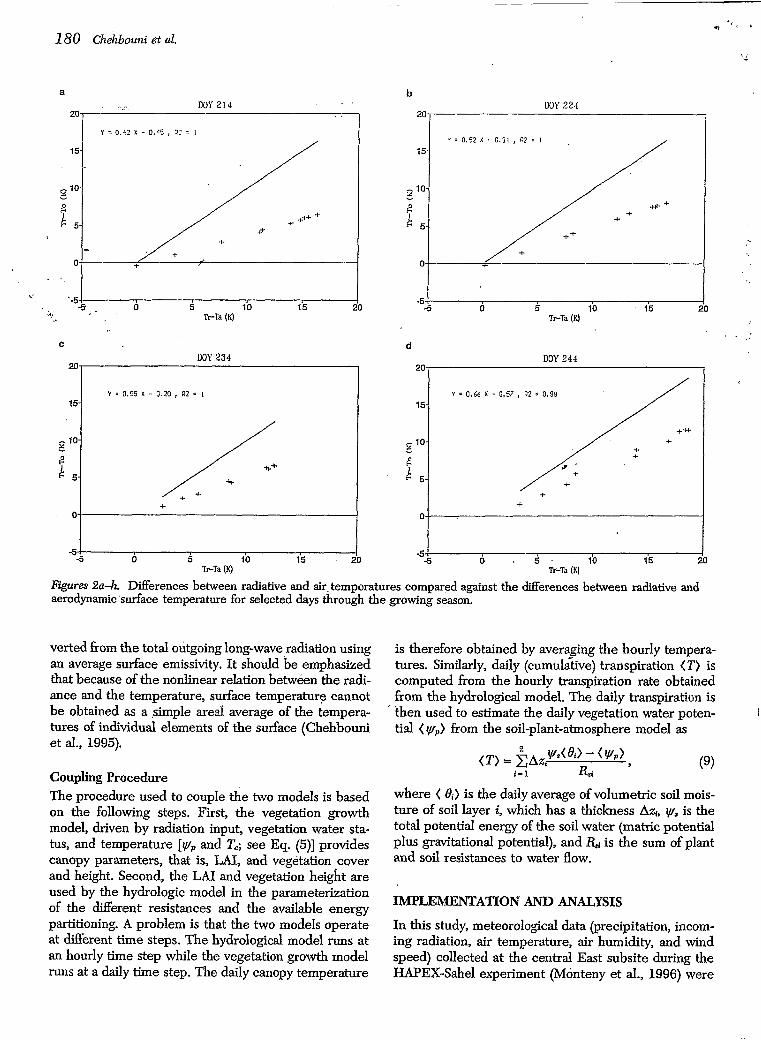
Figures Ba-h. Differences between radiative and air. temperatures compared against the differences between radiative and aerodynamic surface temperature for selected days through the growing season.

verted from the total outgoing long-wave radiation using an average surface emissivity. It should be emphasized that because of the nonlinear relation betwken the radi- ance and the temperature, surface temperature cannot be obtained as a simple area1 average of the temperatures of individual elements of the surface (Chehbouni et al., 1995).

Coupling Procedure The procedure used to couple the two models is based on the following steps. First, the vegetation growth model, driven by radiation input, vegetation water status, and temperature [y, and Tc; see Eq. (5)] provides canopy parameters, that is, LAI, and vegetation cover and height. Second, the LAI and vegetation height are used by the hydrologic model in the parameterization of the Wer'ent resistances and the available energy partitioning. A problem is that the two models operate at different time steps. The hydrological model runs at an hourly time step while the vegetation growth model runs at a daily time step. The daily canopy temperature

is therefore obtained by averaging the hourly temperatures. Similarly, daiiy (cumulåtive) transpiration (?') is computed from the hourly transpiration rate obtained from the hydrological model. The daily transpiraticin is then used to estimate the daily vegetation water potential ( y,) from the soil-plant-atmosphere model as

, .

(9)

where ( Bi) is the daily average of volumetric soil moisture of soil layer i, which has a thickness Azi, v/s is the total potential energy of the soil water (matric potential plus gravitational potential), and & is the sum of plant and soil resistances to water flow.

IMPLEMENTATION AND ANALYSIS

In this study, meteorological data (precipitation, incom- ing radiation, air temperature, air humidity, and wind speed) collected at the central East subsite during the HAPEX-Sahel experiment (Monteny et al., 1996) were

Radiative and Aerodynamic Surface Temperatures over Sparse Vegetation 181

10-

8-

6-

B - 4-

.l

2-

0-

e DOY 254

20

15- Y = 0.65 S - O. 16 , R2 : 0.99

Y 0.b9 k r 0.67, R2 = 6.54

I . I

-2 O 2 4 6 a 10 TrTa (e)

-24

f DOI’ 264

10

Y : 3.62 x + 2.27. U? -. c.5:

2 i O

-2-1 -2 O 2 4 6 8

Tr-Ta (K)

h

I

J I - .

- .

Figures Sa-h. Continued.

used to implement the above scheme. As mentioned above, the objective was to investigate the differences between aerodynamic and radiative surface temperatures over partial canopy cover conditions. Thus, this analysis was confined to the part of vegetation cycle in which values of fractional cover ranged from about 5% to BO%, which correspond for grass to values of LAI ranging from about 0.05 to about 0.95 (see Table 1). These conditions occurred from day of the year (DOY) 212 to DOY 288.

In Figure 1, the day time hourly differences (from 8:OO to 17:OO LT) between radiative and aerodynamic temperatures are plotted for a period ranging from DOY 212 to DOY 288. One can see in this figure that the differences between radiative and aerodynamic surface temperatures are of suf€icient magnitudes that any attempt to ignore them will necessarily lead to erroneous estimates of sensible heat flux. This actually confirms Ifle results reported by Stewart et al. (1989) and Kustas (1990). It can be also noted that daily as well as seasonal variations of these differences do not present any apparent pattern. This may negate any possibility of deriving

aerodynamic surface temperatwe solely from radiative surface temperature, but our objective here is not to establish a direct relationship between radiative and aerodynamic temperatures.

In Figures 2a-h, day time hourly differences between radiative and air temperatures are plotted against the differences between radiative and aerodynamic surface temperatures, for eight selected days through the growing season (see Table 1). Despite some scatters towards the end of the growing season, the differences between the aerodynamic and radiative surface temperatures show a linear increase (slope) with increasing surface-air temperature gradient. In this regard, Kustas (1990) also found that the deviation of To from T, grew as the magnitude of T, increased. The slope of the radiative-aerodynamic surface temperature difference with respect t Ó the radiative-air temperature difference is constant for a given day but varies significantly throughout the season.

Since the aerodynamic-air temperature gradient that is required to express sensible heat flux and to correct for the stability, we compute by linear regression

182 Chehbuuni et al.

0.10-

the slope (ß) of the (To- Ta) and (Tr- Ta) gradients for each individual day of the simulation period (from. DOY 212 to DOY 288) as

c' * + + % ,.+#

-;s L

(1-01

In Figure 3, the multitemporal behavior of the coefficient ß through the growing season is compared to the

'variation of leaf area index (LAI). In spite of some scatte?, possibly due to 8. fact that the intercept in *e computation of the regression was set to zero, which

. was not exactly true under cloudy sky conditions, the ' % general tendency is that the coefficient /3 decreases in

:*'a consistent manner with increasing LAI. It should be noted, however, that this pattern is only relevant under partial cover conditions. Under conditions of hlly covered surfaces, the discrimination between aerodynamic and radiative surface temperature is no more pertinent, and thus the coefficientß must ultimately approach the value of 1. This extreme case however is out of the scope of the present study. The fact that the ß coefficient exhibits a consistent relationship with the LAI throughout the study period suggests that a mean exists to parameterize ß with respect to LAI.

Parameterization Development A subdata set made up of 21 points randomly selected from the entire data set (76 days), was used to develop the following relationship between ß and LAI:

where L is an empirical factor that was set by least squares regression to a value of 1.5. The remaining data set (55 days) was then used to test the performance of the above relationship. Figure 4 presents a comparison between original ß values (obtained by regression) and those simulated using Eq. (11). In spite of some scatter as discussed previously, the agreement between the data and the simulation is fairly good.

By combining Eq. (10) and (ll), aerodynamic-air temperature gradient, which is the gradient required for sensible heat flux formulation, can be expressed in terms of radiative-air temperature one as

The formulation in Eq. (12) was then used to express sensible heat flux. Figure 5 presents a cross-plot between the original, hourly based, sensible heat flux obtained by the coupled model (called here the original one) and that formulateld using To - Ta from Eq. (12) for the remaining 55 days of the data. It can be seen that this parameterization r,eproduces fairly accurately the original sensible heat flux. The root mean square error

BP:¿

o.6o] ++

+ 2

E""] il 0.20

: + * + + + +a? * + ++

.. . + ++

f

1 .o0

0.90

0.80

0.70 I

0.60 2

0.50 i

0.40 ?i

0.30

0.20

0.10

-

-

Y O 0

Figure 3. Comparison between the multitemporal behavior .'

of the coefficient ß values and the leaf area index.

(RMSE) between simulated and original sensible heat flux values was about 30 W m-'.

To validate the performance of this approach, Bowen ratio-based surface fluxes data collected over the herbaceous subsite during .the HAF'EX-Sahel experiment were used [see Monteny et al. (1996) for measurements description]. In Figure 6, values of sensible heat flux corresponding to 14:OO LT (which is approximately the AVHRR time overpass in Niger) are compared, for a period of about 60 days, to those simulated using the above approach: Agreement between observed and simulated values are satisfactory, the RMSE was about 43 W m-'. The result obtained here suggests that sensible heat flux can be accurately estimated if radiative surface temperature, air temperature, and LAI ' are known. This is of interest, since T, and LAI can be potentially obtained from remote sensing. However, the

* Figure 4. Comparison between original ß values (obtained by regressions) and those obtained by the parameterization described in Eq. (11).

0.70

0.60

F 0.50

0.40

0.30

- A F

L Y

i 0.20

0.10

0.og L

Y : 0.94 X t 0.025 , P? y O.fi5 ++

I

I 2iO &O 230 240 250 &O 270 280 290 lXlY

+ Original - Simulation

. ',

I

- - -

Radiative and Aerodynamic Sulface Temperatures over Sparse Vegetution 1 83

. i

+/ y = 1.01 x - 2.41 , R2 i 0.88

' .- !??í:o0 -50 O 50 100 150 200 250 300 350 400

Oridna1 Scnsilrle IIcnl Flux (lV/inZ) I 1,

Figure 5. Cross-plot between original sensible heat flux (obtained by the coupled models) and that obtained using parameterization in Eq. (12).

relationship derived here may be site-specific since it depends on the fitted L factor.

Application to Remotely Sensed Spectral Vegetation Index To investigate the extent to which a remotely sensed spectral vegetation index can be combined with remotely sensed radiative surface temperature to derive accurate values of sensible heat flux over sparsely vegetated surfaces, radiative transfer models were used in. conjunction with the coupled models to simulate the multitemporal behavior of surface reflectances in the RED and near-infrared (NIR) regions. The radiative transfer model used in this investigation assumes that the scene reflectance in a given waveband and at any day of the season can be represented by a simple area weighted average of the reflectances of dry biomass, green biomass, and soil (LoSeen et al., 1995). The model

Figure 6. Comparisons between Bowen ratio based sensible heat flux and that obtained using the parameterization in Eq. (12) at 14:OO LT for about 60 days.

Hapex Sahel Data 400,

- 2004 i

- 1 o o - v , -100 -50 6 5b I60 l i 0 260 230 360 330 4

Bown ratio based Eenrible heat flux

of Hapke (1981) has been used to parameterize the soil reflectance. Parameters needed to run this model were obtained from the literature (Jacquemoud et al., 1992). Green and dry canopy reflectances were computed using the SAIL model (Verhoef, 1984; 1985). The main parameters needed to run the SAIL model are LAI, leaf angle distribution (LAD), and leaf optical properties. for this study, a spherical distribution was assumed for the leaves. The leaf optical properties were computed using the PROSPECT model (Jacquemoud and Baret, 1990). Finally, the LAI was given by the vegetation growth model. Surface reflectances in the RED and NIR regions were simulated during the study period (from DOY 212 to DOY 288) using the NOAA-AVHRR spectral and geometrical configurations. Since no direc-'. - tional correction was performed in this study, data corresponding to large view angle, that is, larger than 40°, were not used. RED and NIR reflectances were used to compute the MSAVI (modified soil adjusted vegetation index) as

. "

'

. -'

.

'

(1 +A) > (13) RED - NIR MSAVI =

RED f NIR + A

where A is a self adjusting factor defined to adapt the soil noise correction to the proportion of soil seen by the sensor (Qi et al., 1994). A is given by the expression

A = 1 - 2 NIR-RED(RED - 1.06 NIR). (14) . NIR+RED

In this study we have considered MSAVI as the vegetation index to use since it was found to be less sensitive to soil brightness variations including shadows than other spectral vegetation indices (Chehbouni et al., 1994). This is of importance since the contribution of bare soil to scene reflectafice is very significant for partially covered surfaces.

In Figure 7, the multitemporal variation of MSAVI is compared to that of the ß coefficient. The behavior of MSAVI with respect to ß is very similar to that of the LAI (refer to Fig. 3). This is not surprising since the LAI is the major input parameter that drives the SAIL model used to simulate surface reflectances. An interesting feature to note in this figure is that the day to day change in the computed MSAVI is much larger than that of the LAI. This is an artifact, mainly due to the effect of view and sun angle variations in the AVHRR configuration used to compute MSAVI (apparent 9-day cycle). Following the discussion in the previous section, there are two possibilities for obtaining sensible heat flux using, radiative surface temperature and MSAVI. One can derive directly a relationship between ß coefficient and MSAVI similar to that in Eq. (ll), or establish a parameterization between LAI and MSAVI first and then use Eq. (12). The second option was chosen here since LAI can be used elsewhere in the surface flux modeling. Previous studies have indicated


- 0.50- 2 .1

f

20.20-

t 0.40- - 0.30-

%

0.70 0.60

Bela MSAVI

-

-0.40

- -0.30 2

r.

-0.20

. < o.,,{

+ f

*; A + t ++

+

it + ++

+ :.. 0.00 ' . 0.00 '. 200 2iO &O 230 240 280 260 270 280 290 300

M Y

Figure 7. Comparison between the multitemporal behavior of the coefficient ß values and the MSAVI.

that a modified Beer's law expression can accurately describe the general relationship between vegetation index and LAI (Asrar et al., 1984; Choudhury et al., 1994). A similar approach to that used to derive Eq. (11) was taken to relate MSAVI to LAI: a part of the data served to calibrate the LAI-MSAVI relationship (the same 21 days mentioned above) and the remaining part to validate it. This leads to a relationship between LAI and MSAVI, which is very similar to that developed by Huete et al. (1985) for cotton data in Arizona:

MSAVI = 0.88 - 0.78 EXP( - 0.6 LAI) . (15) Figure 8 presents a comparison between the original sensible heat flux and that obtained by combining the above relation with Eq. (12). It can be seen that the parameterization reproduces fairly accurately the original flux; the RMSE was about 32 W m-2. This result is almost identical to that shown in Figure 5. This may indicate the goodness of close relationship between LAI and MSAVI, but may also suggest that a part of the noise associated with Eq. (11) might be canceled out with that associated with the view and sun angle effect. The outcome of this study is that there is a real possibility of estimating accurately sensible heat flux from sparsely vegetated surfaces using radiative surface temperature and remotely sensed spectral vegetation index. It is important to remember, however, that the results presented here are for simulated surface refi ectances only; further validation with real satellite data under different environmental conditions is needed.

DISCUSSION AND CONCLUSION

Recent advances in remote sensing technology allow estimation of land surface temperature from space with reasonable accuracy. Radiative surface temperature can immediately be used in conjunction with ancillary meteorological data for the estimation of regional surface

/ 400

-100 -50 O 50 100 150 200 250 300 350 4 01iginol sensiblc hmt flux ( W / m 2 )

Figure 8. Cross-plot between original sensible heat flux and that obtained by combining Eqs. (12) and (15).

O

fluxes. However, it became clear that such method is not reliable over spapely vegetated surfaces (Hall et al., 1992; Sellers and HalI, 1992). The problem has been that, over partial-cover conditions, convective flux should not be expressed in terms of radiative surface temperature, but in terms of aerodynamic surface temperature. We note here that the relationship between radiative and aerodynamic surface temperature has been a subject of research for more than 10 years. It has been reported. the adifference between radiative and aerodynamic surface temperature depends on atmospheric stability I unstability and on solar zenith angle, surface soil moisture, and vegetation status.

In this analysis, a hydrologic model coupled with vegetation growth model has been used to investigate the differences between aerodynamic and radiative surface temperatures over partially covered surfaces. One can argue that there is no need for such a coupling to -address the above issue. This same analysis can certainly be performed using only the hydrological model. How- ever, it is not realistic for the same vegetation type, to vary for example, the leaf area index while keeping the vegetation height and the fractional cover constant. Thus, the only possibility is to perform an univariate analysis, but it is somehow restrictive.

Our results have shown that the ratio between radiative-air and aerodynamic-air temperature differences is intimately related to LAI. This is actually not surprising since the LAI is pertinent parameter charac- terizing the vegetation status but is not used in one- layer-based sensible heat flux estimations, whereas it plays a key role in the determination of bulk boundary- layer resistance in the two-layer-based schemes. Thus, LAI should be included in any attempt toi derive aerodynamic-air temperature gradient from radiative-air temperature gradient, over sparsely vegetated surfaces (Pré- vot et al., 1994).

One may argue that the ratio P should also depend on surface soil moisture. Surface soil moisture is certainly a critical parameter that controls the partitioning of available energy at surface into sensible and latent heat flux, However, radiative surface temperature, which represents the signature of an equilibrium of the surface, is directly controlled by surface soil moisture. Therefore, we feel that the dependence o f ß on soil moisture is through the surface temperature. A parameterization involving radiative surface temperature, air temperature, and LAI has been developed here to formulate sensible heat flux. The simulations showed that

i this parameterization can be successful in estimating sensible ..heat flux over a partially vegetated surface. Additionally, the performance of this approach has been verified using Bowen ratio based sensible heat flux, where the RMSE was not very high comparatively to the error associated with the measurements over such complex terrain (Lloyd et al., 1996). The performance of this approach has been also confirmed elsewhere using data taken over shrub and cotton canopies (Cheh- bouni et al., 1996). Nonetheless further studies are needed to test the generality of Eq. (ll), and to investigate how the L parameter changes with vegetation type and structure.

Finally, the radiative transfer model simulations showed that there is a real potential to remotely estimate sensible heat flux. The simplicity of this approach combined with the availability of long term satellite data (i.e., AVHRR) makes it easy to incorporate the approach into energy balance models to investigate spatial and temporal changes in energy fluxes over arid and semiarid lands. However, correction of directional as well as atmospheric effects for both surface reflectances and temperature is needed before this approach can be performed operationally, but this represents one of our future research objectives. We will also investigate the extent to which the L factor in Eq. (11) can be better characterized using multidirectional data. Finally additional field data over different arid surfaces are needed for testing the consistency of the approach.

This study m s conducted in part at the ]et Propulsion Labora- tory UPL), California Institute of Technology, under contract with the National Aeronautics and Space Administration (NASA). This research is within the framework of the NASA-EOS IDS Project (NAGW 2425). Funding was provided by NRC, ORSTOM, and the French Remote Sensing Program.

’.

REFERENCES

Asrar, G., Fuchs, M., Kanemasu, E. T., and Hatfield, J. L. (1984), Estimating absorbed photosynthetic radiation and leaf area index from spectral reflectance in wheat, Agron. j . 76:300-306.

I .

Brutsaert, W. (1982), Evaporation into the Atmosphere, Reidel, Boston, 299 pp.

Chamberlain, A. C. (1968), Transport of gases to and from surfaces with bluff and wavelike roughness elements, Quart. J. Roy. Meteorol. Soc. 94:18-332.

Chehbouni, A., Kerr, Y. H., Qi, J., Huete, A. R., and Sorooshian S. (1994), Toward the Development of a Multidirectional Vegetation Index, Water Resour. Res. 30:1339-1349.

Chehbouni A., Njoku, E. G., Lhomme, J. P., and Kerr, Y. H. (1995), Approaches for Averaging Surface Parameters and . Fluxes over heterogeneous surfaces, 1. Climate 8(5):1386- 1393. . I

Chehbouni A., LoSeen, D., Njoku, E. C., Lhomme, J. P., Monteny B., and Kerr, Y. H. (1996), Estimation of sensible heat flux over sparsely vegetated, J. Hydrol. HAPEX-Sahel special issue, forthcoming.

Choudhury, B. J., and Monteith, J. L. (1988), A four-layer model for the heat budget of homogeneous land surfaces, Quart. j . Roy. Meteorol. Soc. 114:373-398.

Choudhury, B. J., Nizam, U, A., Idso, S. B., Reginato, R. J., and Daughtry, C. S. T. (1994), Relations between evaporation coefficients and vegetation indices studied by model simulations, Remote Sem. Environ. 5O:l-17.

Coutorbe, J. P., Lebel, T., Tinga, A., et al. (1993), HAPEX- Sahel: a large scale study ofcland-atmosphere interactions in the semiarid tropics, Ann. Geophys. 12:53-64.

Hall, G. H., Huemmrich, K. F., Goetz, S. J,, Sellers, P. J.. and Nickeson, J. E. (1992), Satellite remote sensing of surface energy balance: success, failure and unresolved issues in FIFE, J. Geophys. Res. 97:19061-19089.

Hapke, B. (198J), Bidirectional reflectance spectroscopy. I. Theory, 1. Geophys. Res. 863039-3054.

Huete, A. R., Jackson, R. D., and Post, D. F. (1985), Spectral reponse of plant canopy with different soil backgrounds, Remote Sens. Environ. 15:155-165.

Jackson, R. D. (1985), Evaluating Evapotranspiration at local and regional scales, Proc. IEEE 73:1086-1095.

Jacquemoud, S., and Baret, F. (.1990), PROSPECT: a model of leaf optical properties spectra, Remote Sens. Environ.

Jacquemoud, S., Baret, F., and Hanocq, J. F. (1992), Modeling spectral and bidirectional soil reflectance, Remote Sens. Environ. 41:123-132.

Kalma, J. D., and Jupp, D. L. B. (1990), Estimating evaporation from pasture using infrared thermometry: evaluation of a one-layer resistance model, Agric. For. Meteorol. 51:223- 246.

Kustas, W. P. (1990), Estimates of evapotranspiration with one- and two-layer model of heat transfer over partial canopy cover. I. Awl . Meteorol. 49:704-715.

Kustas, W. P., Choudhury, B. J., Moran, M. S., et al. (1989), Determination of sensible heat flux over sparse canopy using thermal infrared data, Agric. For. Meteurol. 44:197- 216. ,

Lloyd, C. R., Bessemoulin, P., Cropley, F. D., et al. (1996), A comparison of surface fluxes at the Hapex-Sahel Fallow bush sites,]. Hydrol., HAPEX-Sahel special issue (in press).

Lhomme, J. P., Troufleau, D., Monteny, B. A., Chehbouni, A., and Bauduin, S. (1996), Sensible heat flux and radiometric surface temperature over sparse sahelian vegetation: a

~

’

34:75-91.


model for the kB-' parameter, J. Hydrol., HAPEX-Sahel special issue, forthcoming.

LoSeen, D., Mougin, E., Rambal S., Gaston, A., and Hiernaux, F. j i G % j , PI regionai saheiian grassian-à möàëí tö be coii- pled with satellite multispectral data. II: Relations with spectral measurements, Remote Sens. Environ. 53:194-206.

LoSeen, D., Chehbouni, A., Njoku, E. G., Saatchi, S., Mougin, E., and Monteny, B. (1996), A coupled Biomass production, water and surface energy balance model for remote sensing application in semiarid grasslands, Agric. For. Meteorol. (in press).

Moran, M. S., Kustas, W. P., Vidal, A., Stannard, D. I., Blan- ' ford, J. H., and Nichols, W. D. (1994), Use ofground-based

remotely sensed data for surface energy balance evaluation of a semi-arid rangeland, Water Resour. Res. 30:1339-1349.

Monteny, B. A., Lhomme, J. P., Chehbouni, A., et al. (1996), The role of the Sahelian biosphere on the water and COZ cycle during the HAPEX-Sahel experiment, J, Hydrol., HAPEX-Sahel special issue, forthcoming.

Mougin, E., LoSeen, D., Rambal, S., Gaston, A., and Hiernaux, P. (1995), A regional sahelian grassland model to be coupled with satellite multispectral data. I. Validation, Remote Sens. Enuiron. 52:181-193.

Prévot, L., Brunet, Y., Paw, U. K. T., and Seguin, B. (1994), Canopy modelling estimating sensible heat flux firom thermal infrared measurements, in Proc. Workshop on Thermal Remote Sensing of the Energy and Water Balence over Vegetatwn in Conjunction with Other Sensors, La Londe- Les Maures, France, 20-23 September 1993, CEMAGREF ed., pp. 17-22.

I

I

*-

Qi, J., Chehbouni, A., Huete, A. R., Kerr, Y. H., and Soroos- hian, S. (1994), A modified soil adjusted vegetation index, Remote Sens. Environ. 48(2):119-126.

Sellers, 1. j:, and Iiail, F. G. (i%Zj, =FE in i992: resuirs, scientific gains, and future research directions, J. Geophys. Res. 97:19,091-19,109.

Shuttleworth, W. J., and Gurney, R. J. (1990), The theoretical relationship between foliage temperature and canopy resistance in sparse crops, Quart. J. Roy. Meteorol. Soc. 116:

Shuttleworth, W. J., and Wallace, J. S. (1985), Evaporation from sparse crops-an energy combination theory, Quart. J. Roy. Meteorol. Soc. 111339-855.

Stewart, J. B., Shuttleworth, W. J., Blyth, K., and Lloyd, C. D. (1989), FIFE: a comparison between aerodynamic surface temperature and radiometric surface temperature - over sparse prairie grass, in 19th Conf: Agric. For. Meteorol., Charleston, SC, March 1989, pp. 144-146.

497-519.

Sun, J., and Mahrt, L. (1995), Detemination of surface fluxes I

from the surface radiative temperature, J. Atm Sci. 52(8): "

6

1096-1106. Troufleau, D., Lhomme, J.-P., Monteny, B., and Vidal, A.

(1996), Sensible heat flux and radiometric surface temperature over sparse sahelian vegetation: is the kB-' a relevant parameter, J. Hydrol. (in pjess).

Verhoef, W. (1984), Light scattering by leaf layers with application to canopy reflectance modeling: the SAIL model, Remote Sens. Enuiron. 16:125-141.

Verhoef, W. (1985), Earth observation modeling based on layer scattering matrices, Remote Sens. Enuiron. 17:165- 178.

Examination of the difference between radiative and aerodynamic ...

Documents

Transcript of Examination of the difference between radiative and aerodynamic ...