Examination of the Bouchet–Morton Complementary...

Examination of the Bouchet–Morton Complementary Relationship Using a MesoscaleClimate Model and Observations under a Progressive Irrigation Scenario

MUTLU OZDOGAN

NASA GSFC, Greenbelt, Maryland

GUIDO D. SALVUCCI AND BRUCE T. ANDERSON

Department of Geography, Boston University, Boston, Massachusetts

(Manuscript received 10 November 2004, in final form 29 April 2005)

ABSTRACT

The complementary relationship between actual and potential evaporation over southeastern Turkey wasexamined using a mesoscale climate model and field data. Model simulations of both actual and potentialevaporation produce realistic temporal patterns in comparison to those estimated from field data; asevaporation from the surface increases with increasing irrigation, potential evaporation decreases. This is inaccordance with the Bouchet–Morton complementary relationship and suggests that actual evapotranspi-ration can be readily computed from routine meteorological observations. The driving mechanisms behindirrigation-related changes in actual and potential evaporation include reduced wind velocities, increasedatmospheric stability, and depressed humidity deficits. The relative role of each in preserving the comple-mentary relation is assessed by fitting a potential evaporation model to pan evaporation data. The impor-tance of reduced wind velocity in maintaining complementarity was unexpected, and thus examined furtherusing a set of perturbation simulation experiments with changing roughness parameters (reflecting growingcotton crops), changing moisture conditions (reflecting irrigation), and both. Three potential causes of windvelocity reduction associated with irrigation may be increased surface roughness, decreased thermal con-vection that influences momentum transfer, and the development of anomalous high pressure that coun-teracts the background wind field. All three are evident in the mesoscale model results, but the primarycause is the pressure-induced local wind system. The apparent necessity of capturing mesoscale dynamicalfeedbacks in maintaining complementarity between potential and actual evaporation suggests that a theorymore complicated than current descriptions (which are based on feedbacks between actual evaporation andtemperature and/or humidity gradients) is required to explain the complementary relationship.

1. Introduction

It is widely accepted that regional evapotranspirationfrom land surfaces is difficult to estimate and remainsone of the most poorly understood components of thehydrologic cycle (Entekhabi et al. 1999). In part, thisdifficulty stems from lack of reliable data on soil mois-ture, especially in highly variable surfaces. Addition-ally, most routine methods to estimate evapotranspira-tion require hard-to-obtain parameters such as turbu-lent transfer coefficients and stomatal conductances.Thus, evaporation estimation methods that avoid the

use of rarely available soil moisture data and are simpleenough to be used with routinely available meteoro-logical data are highly desirable.

One such method is the complementary relationship(hereafter CR) first proposed by Bouchet (1963) andfurther developed by Morton (1965). Originally basedentirely on heuristic arguments, the theory of comple-mentarity has found wide support in the literature boththrough comparison to other methods that estimateevapotranspiration (Parlange and Katul 1992; Quallsand Gultekin 1997) and through analysis based on me-teorological observations and/or modeling results(Hobbins et al. 2001; Sugita et al. 2001; Ozdogan andSalvucci 2004; Hobbins et al. 2004). Other recent re-search is focused on finding a more physical foundationfor the CR (e.g., Kim and Entekhabi 1997; Szilagyi2001).

Corresponding author address: Mutlu Ozdogan, NASA GSFC,Code 614.3, Greenbelt, MD 20771.E-mail: [email protected]

APRIL 2006 O Z D O G A N E T A L . 235

© 2006 American Meteorological Society

JHM485

The purpose of the study presented herein is to in-vestigate the validity of the CR in southeastern Turkeywith the help of a mesoscale climate model as well aswith meteorological data. The CR was evaluated withinthe climate model by performing 10-day midsummersimulations to determine the changes in hydrologicfluxes under a progressive irrigation development sce-nario. The model, which forecasts regional meteoro-logical and surface conditions, implicitly captures thefeedbacks between potential and actual evaporation byupdating the temperature and moisture fields, both atthe surface and in the overlying atmosphere, which sub-sequently moderates the interaction between the two.This makes the model a reasonable forecasting tool forthis region and a reasonable tool for supporting or con-tradicting the theory of complementarity. The CR wasfurther analyzed by estimating the terms of the Penmanequation [including the Monin–Obukhov (1954) (M–O)stability parameters] that was calibrated to measuredpan evaporation. Because M–O characterization re-quires specification of the sensible heat flux (H), asimple land surface energy balance was computed toestimate H in conjunction with the potential evapora-tion equation.

By combining the results from the climate model andmeteorological data, it was possible to (i) test the CRpurely in the mesoscale model; (ii) compare potentialevaporation estimates between the climate model, panevaporation data, and calibrated potential evaporationequations; (iii) estimate the M–O scaling variables(which include instability) for comparing environmen-tal variables such as wind speed and humidity betweenthe climate model and observations; (iv) have a cali-brated potential evaporation equation with which sen-sitivity analyses could be performed to explore the rela-tive importance of variables like humidity and windspeed for maintaining complementarity; and (v) ex-plore the larger-scale, dynamical feedbacks controllingthe wind speed decreases reported in Ozdogan and Sal-vucci (2004). As an example of a unique long-runningexperiment, the data collected throughout the exten-sive irrigation development projects in southeasternTurkey provide an opportunity to perform and evaluateeach of these tasks.

2. The complementary relationship

The CR states that under constant energy input andaway from sharp discontinuities there exists a comple-mentary feedback mechanism between actual (Ea) andpotential (Ep) evapotranspiration that causes changesin each to be complementary, that is, a unit decreasein Ea causes a unit increase in Ep. Here, Ep is definedas the evapotranspiration given by the Penman equa-

tion using meteorological variables under prevailing at-mospheric conditions. In contrast, a sufficiently moistuniform surface evapotranspiring at the potential rateunder steady-state conditions would be defined asequilibrium, or wet-environment, evapotranspiration(Ew) [after Morton (1965) and Brutsaert and Stricker(1979)]. Bouchet (1963) hypothesized that under con-ditions of minimal advection, when Ea, due to limitedwater availability, falls below its potential rate (Ew), acertain amount of energy (Q) would become available:

�Ew � �Ea � Q. �1�

This excess energy not used for evapotranspirationwould then warm the atmosphere. Increased air tem-perature due to this warming and decreased humiditydue to reduced evapotranspiration would then lead to a“new” potential evapotranspiration (Ep) that is largerthan Ew by the amount Q:

�Ew � Q � �Ep. �2�

Combining Eqs. (1) and (2) lead to the complementaryrelationship (Fig. 1)

�Ea � 2�Ew � �Ep. �3�

If water availability at the surface is increased—for ex-ample, through irrigation—the reverse process occurs,and Ep decreases as Ea increases. Thus, potentialevaporation measured over a region becomes both theresult and cause of actual evaporation measured overthe same region.

In evaluating the CR, Ep is commonly computed withthe combination equation of Penman (1948) and Ew

with the empirical equation of Priestley and Taylor

FIG. 1. Schematic representation of the CR, where ETa is actualevapotranspiration, ETp is potential evapotranspiration, and ETw

is wet-environment evapotranspiration. The x axis represents in-creasing wetness.

236 J O U R N A L O F H Y D R O M E T E O R O L O G Y VOLUME 7

(1972) for conditions of minimal advection. In this re-search, the CR is evaluated by comparing model-simulated and observed Ep and Ea to those computedby the calibrated Penman equation.

3. Climate model description

The simulation of Ep and Ea under a progressive ir-rigation development scenario was performed using theNational Centers for Environmental Prediction (NCEP)Regional Spectral Modeling (RSM) system (Juang andKanamitsu 1994; Juang et al. 1997). The NCEP globalto regional modeling system contains two compo-nents—a low-resolution Global Spectral Model (GSM)and a Regional Spectral Model with multiple nests(RSM1 and RSM2). The nesting method is a one-way,noninteractive procedure, designed to calculate re-gional responses (or adjustments) of the RSM to thelarge-scale background fields provided by the coarser-resolution GSM and RSM1, respectively (Juang andKanamitsu 1994; Juang et al. 1997). The multinestingallows the model system to capture the finescale fea-tures such as changing surface conditions (e.g., en-hanced irrigation) in the RSM, while still incorporatingthe development of large-scale synoptic features in theGSM. The resolution of the GSM is triangular-62 (T62,approximately 200 km); the resolutions for the RSM1and RSM2 are chosen as 25 and 10 km, respectively, forthe study region. A portion of the RSM2 domain overthe Harran Plain is shown in Fig. 2.

Particularly important in this study is the Land Sur-face Model (LSM) though which the coupled transportof momentum, heat, and moisture across the soil andvegetation layers are computed. The LSM coupled tothe RSM is an early version of the NOAH land surfacescheme as described in Chen et al. (1996). The NOAHLSM is a one-dimensional model with explicit vegeta-tion canopy, soil hydrology, and soil thermodynamics.It employs a homogeneous soil scheme (with two lay-ers) and vegetation type where vegetation fraction (�f)is set at 0.7 for each grid. The model simulates soilmoisture, soil temperature, skin temperature, canopywater contents, and the energy and water flux terms ofthe surface energy and water balance. The turbulentflux computations use expressions derived from Monin–Obukhov similarity theory. In particular, evaporation(Ea) is computed as the sum of three parts: bare soilevaporation, canopy re-evaporation, and transpiration,each bounded by the potential evaporation (Ep), whichitself is calculated using a Penman-based energy bal-ance approach supplemented by atmospheric stabilitycorrections (Mahrt and Ek 1984). For further details,the reader is referred to Chen et al. (1996).

The planetary boundary layer (PBL) processes

(Hong and Pan 1996) are based on vertical diffusion inwhich the surface layer and PBL are coupled using aprescribed profile with similarity-based scale param-eters. PBL height is computed iteratively by first com-puting the height without accounting for virtual tem-perature instability near the surface; from this estimate,calculations of vertical velocities can be obtained,which then allow estimation of the virtual temperatureinstability and subsequently modified boundary layerheights (Hong and Pan 1996). The diffusion parametersfor momentum and mass (evaporation) are then deter-mined from the boundary layer height using the pre-scribed profile shape.

As described in section 2, the CR arises from thefeedback mechanisms within the PBL. One of thestrengths of using a mesoscale climate model to evalu-ate CR is the relatively complete accounting of inter-actions between the surface and the PBL as well asbetween PBL and the free atmosphere. Thus, keyphysical processes such as radiative forcing (both sur-face and atmospheric) and stability of the atmosphereare continuously updated as a function of changing sur-face conditions (i.e., irrigation in these experiments)such that their effects on Ea and Ep are accounted for.This approach is in contrast with some earlier model-based evaluations of the CR using simple mixed-layermodels (e.g., McNaughton and Spriggs 1989; Lhomme1997).

FIG. 2. Representation of irrigated fields within the RegionalSpectral Model. The graphic on the left shows the irrigated Har-ran Plain as seen by the Landsat satellite. The dark gray colorsindicate the presence of irrigated croplands. The graphic on theright shows grid box representation of the irrigated fields withinthe model. The location of the Koruklu meteorological station(black star) and grids 44, 45, 54, and 55 (darker gray) are shownfor reference. Only a portion of the full modeling domain isshown. The bottom edge of each graphic is �40 km.


4. Experimental design

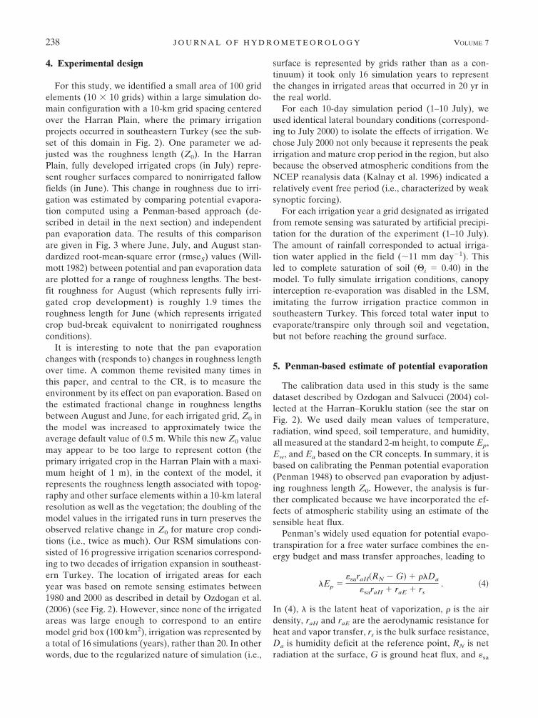
For this study, we identified a small area of 100 gridelements (10 � 10 grids) within a large simulation do-main configuration with a 10-km grid spacing centeredover the Harran Plain, where the primary irrigationprojects occurred in southeastern Turkey (see the sub-set of this domain in Fig. 2). One parameter we ad-justed was the roughness length (Z0). In the HarranPlain, fully developed irrigated crops (in July) repre-sent rougher surfaces compared to nonirrigated fallowfields (in June). This change in roughness due to irri-gation was estimated by comparing potential evapora-tion computed using a Penman-based approach (de-scribed in detail in the next section) and independentpan evaporation data. The results of this comparisonare given in Fig. 3 where June, July, and August stan-dardized root-mean-square error (rmseS) values (Will-mott 1982) between potential and pan evaporation dataare plotted for a range of roughness lengths. The best-fit roughness for August (which represents fully irri-gated crop development) is roughly 1.9 times theroughness length for June (which represents irrigatedcrop bud-break equivalent to nonirrigated roughnessconditions).

It is interesting to note that the pan evaporationchanges with (responds to) changes in roughness lengthover time. A common theme revisited many times inthis paper, and central to the CR, is to measure theenvironment by its effect on pan evaporation. Based onthe estimated fractional change in roughness lengthsbetween August and June, for each irrigated grid, Z0 inthe model was increased to approximately twice theaverage default value of 0.5 m. While this new Z0 valuemay appear to be too large to represent cotton (theprimary irrigated crop in the Harran Plain with a maxi-mum height of 1 m), in the context of the model, itrepresents the roughness length associated with topog-raphy and other surface elements within a 10-km lateralresolution as well as the vegetation; the doubling of themodel values in the irrigated runs in turn preserves theobserved relative change in Z0 for mature crop condi-tions (i.e., twice as much). Our RSM simulations con-sisted of 16 progressive irrigation scenarios correspond-ing to two decades of irrigation expansion in southeast-ern Turkey. The location of irrigated areas for eachyear was based on remote sensing estimates between1980 and 2000 as described in detail by Ozdogan et al.(2006) (see Fig. 2). However, since none of the irrigatedareas was large enough to correspond to an entiremodel grid box (100 km2), irrigation was represented bya total of 16 simulations (years), rather than 20. In otherwords, due to the regularized nature of simulation (i.e.,

surface is represented by grids rather than as a con-tinuum) it took only 16 simulation years to representthe changes in irrigated areas that occurred in 20 yr inthe real world.

For each 10-day simulation period (1–10 July), weused identical lateral boundary conditions (correspond-ing to July 2000) to isolate the effects of irrigation. Wechose July 2000 not only because it represents the peakirrigation and mature crop period in the region, but alsobecause the observed atmospheric conditions from theNCEP reanalysis data (Kalnay et al. 1996) indicated arelatively event free period (i.e., characterized by weaksynoptic forcing).

For each irrigation year a grid designated as irrigatedfrom remote sensing was saturated by artificial precipi-tation for the duration of the experiment (1–10 July).The amount of rainfall corresponded to actual irriga-tion water applied in the field (�11 mm day�1). Thisled to complete saturation of soil (i � 0.40) in themodel. To fully simulate irrigation conditions, canopyinterception re-evaporation was disabled in the LSM,imitating the furrow irrigation practice common insoutheastern Turkey. This forced total water input toevaporate/transpire only through soil and vegetation,but not before reaching the ground surface.

5. Penman-based estimate of potential evaporation

The calibration data used in this study is the samedataset described by Ozdogan and Salvucci (2004) col-lected at the Harran–Koruklu station (see the star onFig. 2). We used daily mean values of temperature,radiation, wind speed, soil temperature, and humidity,all measured at the standard 2-m height, to compute Ep,Ew, and Ea based on the CR concepts. In summary, it isbased on calibrating the Penman potential evaporation(Penman 1948) to observed pan evaporation by adjust-ing roughness length Z0. However, the analysis is fur-ther complicated because we have incorporated the ef-fects of atmospheric stability using an estimate of thesensible heat flux.

Penman’s widely used equation for potential evapo-transpiration for a free water surface combines the en-ergy budget and mass transfer approaches, leading to

�Ep ��saraH�RN � G� � ��Da

�saraH � raE � rs. �4�

In (4), is the latent heat of vaporization, � is the airdensity, raH and raE are the aerodynamic resistance forheat and vapor transfer, rs is the bulk surface resistance,Da is humidity deficit at the reference point, RN is netradiation at the surface, G is ground heat flux, and �sa


is the slope of saturation specific humidity, linearizedaround Ta,

�sa ��

Cp�dQsat

dT �T�Ta

. �5�

Mahrt and Ek (1984) note the importance of atmo-spheric stability on aerodynamic resistance for heat(raH) and vapor (raE) transfer in potential evaporationexplained by Eq. (4). Accordingly, raH and raE werecomputed by

raH,E � �ln�Zr

Z0� � �H,E� 1

ku*. �6�

In (6), Zr is the reference height (2 m), Z0 is the rough-ness length (seasonally varying; see Fig. 3), k is the vonKármán’s constant (0.41), u* is the friction velocity, and H and E are the stability corrections for heat andvapor transfer, respectively, as a function of the Monin–Obukhov length. The details concerning these stabilitycorrection factors are well established and can be foundin Brutsaert (1982) and Garratt (1992). The values foru* are obtained from wind speed at reference height(U2) and roughness length (Z0) as

u* �k * U2

ln�Zr �Z0� � �M. �7�

In (7), M is the stability correction for momentumtransfer as mentioned above. Note that in this study,the roughness length for heat/moisture and momentumare assumed to be identical in resistance correctionterms. Under nonneutral conditions, however, theseroughness lengths may differ up to several orders ofmagnitude as a function of surface temperature overmost natural homogeneous surfaces (Brutsaert 1982;Garratt 1992; Stewart et al. 1994, Brutsaert 1999). Nev-ertheless, given the nature of surface temperature com-puted as a residual of the surface energy balance [Eq.(8)] as well as the extensive calibration procedure de-scribed below, we believe our results are not very sen-sitive to the exact formulation of these resistances.

To incorporate the above stability effects as would befelt by the meteorological site where the evaporationpan is located, the average sensible heat flux from theHarran Plain was estimated. This large-scale flux ishere referred to as the environmental sensible heat flux(HENV) to distinguish it from the sensible heat flux thatwould occur from the pan itself (Hpan). The critical dis-tinction is that we use HENV to estimate the stabilitycorrections and not Hpan, because the pan is too smallto influence the boundary layer. The calibration proce-dure thus required that two land surface energy bal-ances be computed: one for the environment (SEBENV)

and another for the meteorological site (meant to rep-resent the evaporating pan) (SEBmet). In each SEB, thebasic-state variable is the surface temperature (Ts):

�RSW↓�1 � �s� � eS�RLW↓ � �Ts,pan4��

� G � Epan � Hpan � 0, �8�

�RSW↓�1 � �s� � eS�RLW↓ � �Ts,ENV4��

� G � EWB � HENV � 0. �9�

In both of these equations, �s is surface albedo and eS isemissivity; RLW↓ was estimated with expression fromBrutsaert (1982). Again, the principal goal here was tocalculate the terms (via HENV) to account for theeffects of environmental instability on pan evaporation.In Eq. (8), Epan is modeled using a saturated surfacehumidity (these are the values that are compared withthe pan data for estimation of Z0 in Fig. 3). In Eq. (9),on the other hand, evaporation is set to its observedvalue from water balance (EWB), allowing HENV to beestimated as a residual of SEBENV via G and net radia-tion [Eq. (9)]. The stability correction factors computedas a function of HENV are then used within the meteo-rological site-based energy budget to compute fluxesthat corresponded to a unique surface temperature [Eq.(8)]. Note that in order to achieve closure in both SEBs,Eqs. (8) and (9) were solved for Ts,pan and Ts,ENV si-multaneously through iteration because of the implicitdependence of sensible heat in u* (through M) and inraH and raE (through H and E). As alluded to in theprevious section, the whole process was repeated for arange of Z0 estimates until the best fit was obtained

FIG. 3. Standardized rmse between potential and pan evapora-tion data for different roughness length (Z0) values for three sum-mer months in the Harran Plain. The data is the 20-yr average foreach month.


between measured pan evaporation and predictions(Fig. 3). Note that pan evaporation is known to exceedpotential evaporation because of increased water tem-perature as well as ventilation. In Eq. (8), the Tpan vari-able—computed as a residual of SEBmet—partly ac-counts for this elevated temperature effect. Addition-ally, the uncertainty around the surface temperature aswell as the nature of the evaporating pan (not raisedabove the ground surface) at this site suggests less-than-significant ventilation effects. Thus no adjustmentswere made to the pan evaporation data.

6. Evaluation of the complementary relationship

Evaluation of the CR also involves an estimation ofEw, which is calculated based on the concepts proposedby Priestley and Taylor (1972) for conditions of mini-mal advection. These concepts have led to the develop-ment of an equation for potential evaporation given by

�Ew � ��

� � 1�RN � G�. �10�

In (10), the value of the constant �, the well-knownPriestley–Taylor parameter, is reported to be 1.26, al-though it represents the climatological mean. A num-ber of studies have reported that � can range between1.0 and 1.5 (Lhomme 1997; Kim and Entekhabi 1997;Raupach 2000).

For comparison with CR estimates [Eq. (3)], we usedan independent estimate of Ea from Ozdogan et al.(2006) who computed seasonal water use for irrigationin the study area for the period 1980–2001 based onestimates of irrigated acreage from remote sensing.While no actual evaporation measurement was avail-able for validation of computed fluxes, this total sea-sonal irrigation, expressed as [LT�1], was the best in-dependent water-balance-based estimate of Ea.

In evaluating CR, we (i) analyze the changes in Ep

and Ea, simulated by the mesoscale model, for increas-ing surface moisture conditions; (ii) compare the cli-mate model simulations of Ep and Ea to the computed

fluxes from the station data as averaged over the simu-lation period; (iii) perform sensitivity analyses with thecalibrated potential evaporation equation to explorethe relative importance of environmental variables formaintaining complementarity; and (iv) explore thelarger-scale, dynamical feedbacks controlling windspeed changes.

7. Results and discussion

Previous assessments of the ability of the NCEP Re-gional Spectral Model to simulate fluxes have been en-couraging. For example, Anderson et al. (2000, 2004)show that the RSM can successfully simulate the in-traseasonal variations in the climatological summertimehydrologic cycle as well as low-level monsoon windsover the southwestern United States. Brenner (2000)also report good agreement between RSM-simulatedand observed surface wind speed in the eastern Medi-terranean region. Below, the model results, meteoro-logical data, and recalibrated Penman potential evapo-ration equation, as well as the CR, are evaluated for theirrigated plains over southeastern Turkey.

a. Complementary relationship within calibratedPenman equation

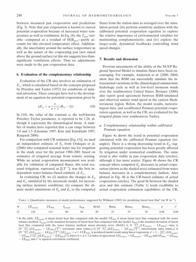
Figure 4a shows the trend in potential evaporationcalculated with the calibrated Penman equation (tri-angles). There is a strong decreasing trend in Ep, sug-gesting potential evaporation has been greatly affectedby irrigation under nonneutral conditions. The sametrend is also visible in pan evaporation data (circles),although it has more scatter. Figure 4b shows the CRconcept where computed Ep decreases as actual evapo-ration (shown as the shaded area) estimated from waterbalance increases in a complementary fashion. Alsoplotted in Fig. 4b is the CR-based estimate of actualevaporation (circles). The good fit between the shadedarea and this estimate (Table 1) lends credibility toactual evaporation estimation capabilities of the CR,

TABLE 1. Quantitative measures of model performance suggested by Willmott (1982) for predicting latent heat flux* (in W m�2).

N LEmodel LEWB Smodel SWB MAE Rmse RmseS RmseU d r2

23 120 112 86 94 30 33 15 29 0.96 0.88

* In the table, LEmodel is mean latent heat flux computed with the model; LEWB is mean latent heat flux computed with the waterbalance method; Smodel is the standard deviation of latent heat flux computed with the model; SWB is the standard deviation of latentheat flux computed with the water balance method; mean absolute error (MAE) is N�1�N

i�1| LEmodel,i � LEWB,i| ; rmse is[N�1�N

i�1(LEmodel,i � LEWB,i)2]0.5; systematic rmse (rmseS) is [N�1�N

i�1(LEmodel,i � LE,WB,i)2]0.5; unsystematic rmse (rmseU) is

[N�1�Ni�1(LEmodel,i � LEWB,i)

2]0.5; LEmodel,i � a � b LEWB,i is predicted model result using linear regression; d � 1 � [�Ni�1(LEmodel,i

� LEWB,i)2/�N

i�1(|LE�model,i| � |LE�WB,i| )2], where 0 � d � 1 is index of agreement; LE�model,i � LEmodel,i � LEWB and LE�WB,i � LEWB,i

� LEWB; and r2 is squared correlation coefficient.


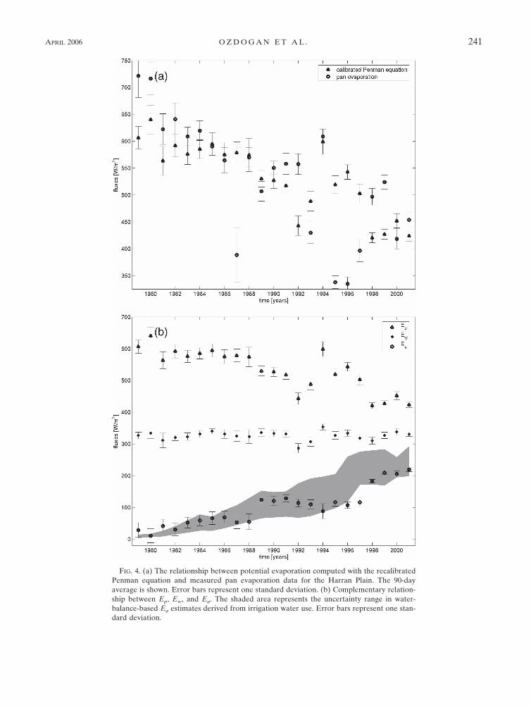
FIG. 4. (a) The relationship between potential evaporation computed with the recalibratedPenman equation and measured pan evaporation data for the Harran Plain. The 90-dayaverage is shown. Error bars represent one standard deviation. (b) Complementary relation-ship between Ep, Ew, and Ea. The shaded area represents the uncertainty range in water-balance-based Ea estimates derived from irrigation water use. Error bars represent one stan-dard deviation.


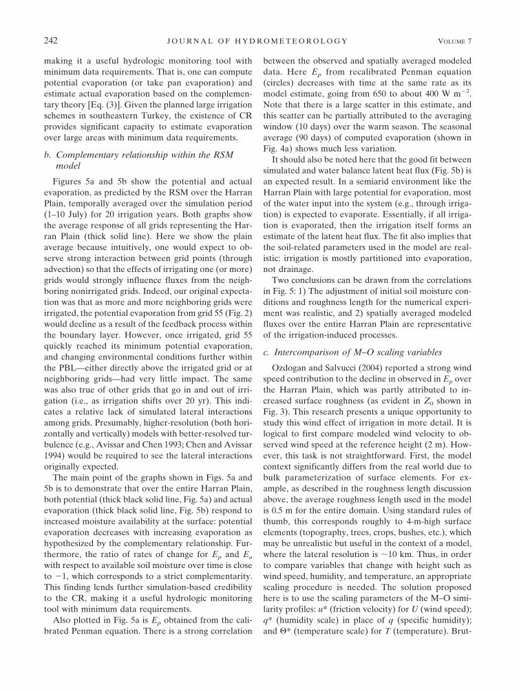
making it a useful hydrologic monitoring tool withminimum data requirements. That is, one can computepotential evaporation (or take pan evaporation) andestimate actual evaporation based on the complemen-tary theory [Eq. (3)]. Given the planned large irrigationschemes in southeastern Turkey, the existence of CRprovides significant capacity to estimate evaporationover large areas with minimum data requirements.

b. Complementary relationship within the RSMmodel

Figures 5a and 5b show the potential and actualevaporation, as predicted by the RSM over the HarranPlain, temporally averaged over the simulation period(1–10 July) for 20 irrigation years. Both graphs showthe average response of all grids representing the Har-ran Plain (thick solid line). Here we show the plainaverage because intuitively, one would expect to ob-serve strong interaction between grid points (throughadvection) so that the effects of irrigating one (or more)grids would strongly influence fluxes from the neigh-boring nonirrigated grids. Indeed, our original expecta-tion was that as more and more neighboring grids wereirrigated, the potential evaporation from grid 55 (Fig. 2)would decline as a result of the feedback process withinthe boundary layer. However, once irrigated, grid 55quickly reached its minimum potential evaporation,and changing environmental conditions further withinthe PBL—either directly above the irrigated grid or atneighboring grids—had very little impact. The samewas also true of other grids that go in and out of irri-gation (i.e., as irrigation shifts over 20 yr). This indi-cates a relative lack of simulated lateral interactionsamong grids. Presumably, higher-resolution (both hori-zontally and vertically) models with better-resolved tur-bulence (e.g., Avissar and Chen 1993; Chen and Avissar1994) would be required to see the lateral interactionsoriginally expected.

The main point of the graphs shown in Figs. 5a and5b is to demonstrate that over the entire Harran Plain,both potential (thick black solid line, Fig. 5a) and actualevaporation (thick black solid line, Fig. 5b) respond toincreased moisture availability at the surface: potentialevaporation decreases with increasing evaporation ashypothesized by the complementary relationship. Fur-thermore, the ratio of rates of change for Ep and Ea

with respect to available soil moisture over time is closeto �1, which corresponds to a strict complementarity.This finding lends further simulation-based credibilityto the CR, making it a useful hydrologic monitoringtool with minimum data requirements.

Also plotted in Fig. 5a is Ep obtained from the cali-brated Penman equation. There is a strong correlation

between the observed and spatially averaged modeleddata. Here Ep from recalibrated Penman equation(circles) decreases with time at the same rate as itsmodel estimate, going from 650 to about 400 W m�2.Note that there is a large scatter in this estimate, andthis scatter can be partially attributed to the averagingwindow (10 days) over the warm season. The seasonalaverage (90 days) of computed evaporation (shown inFig. 4a) shows much less variation.

It should also be noted here that the good fit betweensimulated and water balance latent heat flux (Fig. 5b) isan expected result. In a semiarid environment like theHarran Plain with large potential for evaporation, mostof the water input into the system (e.g., through irriga-tion) is expected to evaporate. Essentially, if all irriga-tion is evaporated, then the irrigation itself forms anestimate of the latent heat flux. The fit also implies thatthe soil-related parameters used in the model are real-istic: irrigation is mostly partitioned into evaporation,not drainage.

Two conclusions can be drawn from the correlationsin Fig. 5: 1) The adjustment of initial soil moisture con-ditions and roughness length for the numerical experi-ment was realistic, and 2) spatially averaged modeledfluxes over the entire Harran Plain are representativeof the irrigation-induced processes.

c. Intercomparison of M–O scaling variables

Ozdogan and Salvucci (2004) reported a strong windspeed contribution to the decline in observed in Ep overthe Harran Plain, which was partly attributed to in-creased surface roughness (as evident in Z0 shown inFig. 3). This research presents a unique opportunity tostudy this wind effect of irrigation in more detail. It islogical to first compare modeled wind velocity to ob-served wind speed at the reference height (2 m). How-ever, this task is not straightforward. First, the modelcontext significantly differs from the real world due tobulk parameterization of surface elements. For ex-ample, as described in the roughness length discussionabove, the average roughness length used in the modelis 0.5 m for the entire domain. Using standard rules ofthumb, this corresponds roughly to 4-m-high surfaceelements (topography, trees, crops, bushes, etc.), whichmay be unrealistic but useful in the context of a model,where the lateral resolution is �10 km. Thus, in orderto compare variables that change with height such aswind speed, humidity, and temperature, an appropriatescaling procedure is needed. The solution proposedhere is to use the scaling parameters of the M–O simi-larity profiles: u* (friction velocity) for U (wind speed);q* (humidity scale) in place of q (specific humidity);and * (temperature scale) for T (temperature). Brut-


FIG. 5. (a) Warm season potential evaporation predicted by the RSM climate model (solidline) and calculated with the observed quantities from the meteorological station (circles) theHarran Plain. Simulated (RSM) potential evaporation was derived by the Land Surface Modelusing a Penman-type approach. Error bars on the observed quantities represent one standarddeviation. (b) Warm season actual evaporation in the Harran Plain predicted by the RSMclimate model (solid line). Also shown are observed quantities from water balance (shadedarea). Simulated (RSM) actual evaporation was predicted using standard surface flux calcu-lations by the Land Surface Model. The shaded area represents the uncertainty range in thewater balance estimate.


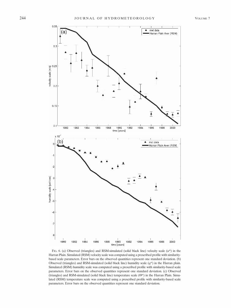
FIG. 6. (a) Observed (triangles) and RSM-simulated (solid black line) velocity scale (u*) in theHarran Plain. Simulated (RSM) velocity scale was computed using a prescribed profile with similarity-based scale parameters. Error bars on the observed quantities represent one standard deviation. (b)Observed (triangles) and RSM-simulated (solid black line) humidity scale (q*) in the Harran plain.Simulated (RSM) humidity scale was computed using a prescribed profile with similarity-based scaleparameters. Error bars on the observed quantities represent one standard deviation. (c) Observed(triangles) and RSM-simulated (solid black line) temperature scale (*) in the Harran Plain. Simu-lated (RSM) temperature scale was computed using a prescribed profile with similarity-based scaleparameters. Error bars on the observed quantities represent one standard deviation.


saert (1982) and Garratt (1992) provide appropriate ex-pressions for profile-based and the flux-based estimatesof these quantities.

Figures 6a–c show the relationship between modeledand observed scaling parameters of the M–O similarityhypothesis as a function of irrigation over the HarranPlain. The time series velocity scale (u*) between themodel and observations agree considerably, suggestingthat both modeled and observed quantities describe asimilar magnitude of changes in wind speed. On theother hand, the humidity scale (q*) shows less agree-ment, indicating that the sensitivity of the model gridand meteorological station to irrigation are different.Nevertheless, these results have important implicationsfor evaluating CR. For example, decreased mixing inthe PBL and, to a lesser degree, depressed humiditydeficit as a function of irrigation are the primary causesof decreased Ep.

Another conclusion that can be drawn from this mea-surement/model agreement is that the comparison be-tween modeled and observed variables is best achievedwhen the absolute heights of measurement and modellevel are taken out of the process via profile scaling.This is particularly useful in cases where the verticalscales of actual and modeled roughness elements differconsiderably due to the lateral resolution of the model.In such cases, the roughness heights used in the modelwill be larger (to include subgrid topographic roughness

effects). For example, when specific humidity data arecompared at the same absolute height (2 m), their sen-sitivity to irrigation is not as pronounced as their scaledequivalents. The results obtained from these two analy-ses thus provide a procedure on how to compare modelresults to observations, especially for variables thatchange with height.

While the relative temperature change is similar,there is a bias between the model estimate of the tem-perature scale (*) and its estimate from field data.This difference stems mainly from the difference in sen-sible heat flux, which in turn is a function of availableenergy. The formulation of available energy (down-welling and upwelling radiation as well as ground heatflux) is different between the RSM model and valida-tion dataset, showing a �150 W m�2 bias. This differ-ence is mostly due to different albedo and emissivitytreatments of the surface [see Ozdogan (2005) for fur-ther discussion].

d. Mechanisms for the complementary relationship

The good correlations between modeled and ob-served fluxes and the height-independent M–O similar-ity parameters also provide an opportunity to learnmore about the mechanisms that maintain complemen-tarity between potential and actual evaporation. To dothis, the Penman equation [Eq. (16)] was rewritten toemphasize the dependence on stability effects:

FIG. 6. (Continued)


Ep� �

�saraH�z, Z0, �U�HENV��

�RN � G� � ��Da�qa�

�saraH�z, Z0, �U�HENV��

raE�z, Z0, �U�HENV�� rs

. �11�

By holding each of the variables in Eq. (11) constantwhile allowing the others to vary over the 23-yr courseof irrigation, the influence of increased evaporation onEp, as heuristically explained by the CR, can be ex-plored in greater detail (Fig. 7).

Results indicate that both wind speed and stabilityeffects are important in maintaining complementarity.For example, when the effects of wind speed are limitedby holding the wind speed constant at its mean value,potential evaporation increases slightly with increasingevaporation (dashed black line, Fig. 7), indicating thatthe decrease in wind speed with irrigation plays a pri-mary role in producing a decrease in potential evapo-ration. Note that this decrease is not in and of itselfenough to reduce actual evaporation, which increasesdue to increases in the overlying land/atmosphere mois-ture gradient. Similarly, if sensible heat flux is held con-stant at its mean (�130 W m�2), then atmospheric sta-bility will remain constant and potential evaporation ishigher than in the control estimate, especially for

higher irrigation years (dashed gray line, Fig. 7). Thislack of increase in stability counteracts the decreasingeffect of wind speed, leading to a neutral/slightly in-creasing trend in potential evaporation over time. Onlywhen the effects of both stability and wind speed aresimultaneously in operation does potential evaporationshow a decreasing trend, indicating that dynamical ef-fects are an important part of the complementarytheory. The effects of decreasing humidity deficit ap-pear to be also important (light gray line, Fig. 7), but insoutheastern Turkey, dynamics are more important formaintaining CR.

e. Possible explanations for wind speed decrease

In general, the relationship between potential andactual evapotranspiration, as described by the CR, hasbeen defined based solely on the degree to which soil/vegetation continuum can satisfy the atmospheric watervapor demand and consequent changes in energy par-titioning at the land–atmosphere interface (e.g., Kimand Entekhabi 1997; Szilagyi 2001). The changes in thisrelationship due to dynamical effects such as windspeed in the presence of irrigation are an unexpectedfinding of this research and merit further discussion.

Two plausible explanations are considered here forthe observed decrease in wind speed. The first irriga-

FIG. 7. Sensitivity of potential evaporation to different input parameters estimated by hold-ing one variable constant at a time within Eq. (11). “Neutral case” is when stability effectshave been removed. See text for details.


tion-related factor is related to surface roughness. Veg-etated surfaces generally add to aerodynamic surfaceroughness, which, in turn, has the potential to slowdown near-surface wind velocities through the in-creases in friction between the low-level atmosphereand surface (Burman et al. 1975; Alpert and Mandel1986).

The second is related directly to soil moisture. Anumber of field experiments as well as modeling studieson the near-surface meteorological effects of inhomo-geneous surface moisture characteristics have shownevidence of locally generated wind systems arising fromdifferential heating of adjacent areas such as irrigatedpatches among dry natural vegetation (Segal et al. 1989;Segal and Arritt 1992; Doran et al. 1995; De Ritter andGallee 1998). Often referred to as “nonclassical meso-scale circulations,” these wind systems are caused bystrong thermal and pressure gradients over the inter-face between wet (irrigated) and dry surfaces, similar tothat of sea-breeze formation. The locally generatedflow due to these adverse gradients (i.e., higher pres-sure over cool irrigated areas) has the potential tocounteract the main flow regime and decelerate thebackground wind velocity (Segal et al. 1989; Doran et

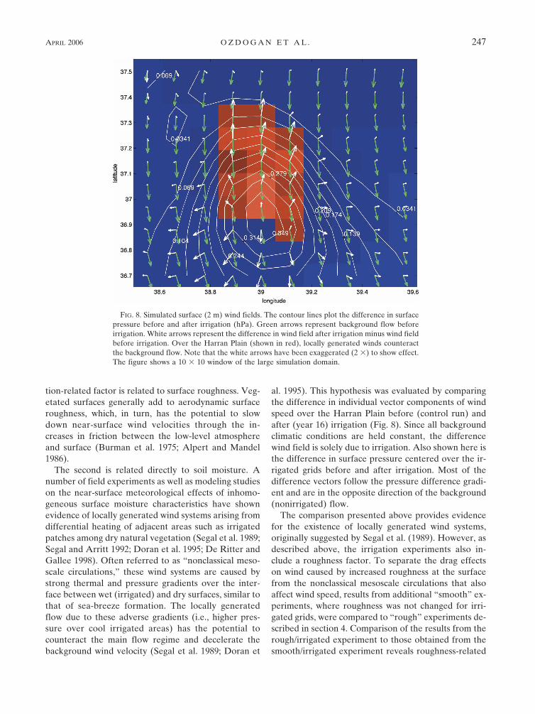
al. 1995). This hypothesis was evaluated by comparingthe difference in individual vector components of windspeed over the Harran Plain before (control run) andafter (year 16) irrigation (Fig. 8). Since all backgroundclimatic conditions are held constant, the differencewind field is solely due to irrigation. Also shown here isthe difference in surface pressure centered over the ir-rigated grids before and after irrigation. Most of thedifference vectors follow the pressure difference gradi-ent and are in the opposite direction of the background(nonirrigated) flow.

The comparison presented above provides evidencefor the existence of locally generated wind systems,originally suggested by Segal et al. (1989). However, asdescribed above, the irrigation experiments also in-clude a roughness factor. To separate the drag effectson wind caused by increased roughness at the surfacefrom the nonclassical mesoscale circulations that alsoaffect wind speed, results from additional “smooth” ex-periments, where roughness was not changed for irri-gated grids, were compared to “rough” experiments de-scribed in section 4. Comparison of the results from therough/irrigated experiment to those obtained from thesmooth/irrigated experiment reveals roughness-related

FIG. 8. Simulated surface (2 m) wind fields. The contour lines plot the difference in surfacepressure before and after irrigation (hPa). Green arrows represent background flow beforeirrigation. White arrows represent the difference in wind field after irrigation minus wind fieldbefore irrigation. Over the Harran Plain (shown in red), locally generated winds counteractthe background flow. Note that the white arrows have been exaggerated (2 �) to show effect.The figure shows a 10 � 10 window of the large simulation domain.


Fig 8 live 4/C

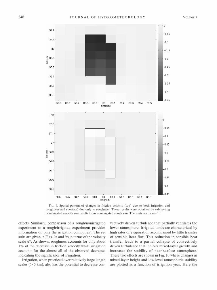
effects. Similarly, comparison of a rough/nonirrigatedexperiment to a rough/irrigated experiment providesinformation on only the irrigation component. The re-sults are given in Figs. 9a and 9b in terms of the velocityscale u*. As shown, roughness accounts for only about1% of the decrease in friction velocity while irrigationaccounts for the almost all of the observed decrease,indicating the significance of irrigation.

Irrigation, when practiced over relatively large lengthscales (� 5 km), also has the potential to decrease con-

vectively driven turbulence that partially ventilates thelower atmosphere. Irrigated lands are characterized byhigh rates of evaporation accompanied by little transferof sensible heat flux. This reduction in sensible heattransfer leads to a partial collapse of convectivelydriven turbulence that inhibits mixed-layer growth andincreases the stability of near-surface atmosphere.These two effects are shown in Fig. 10 where changes inmixed-layer height and low-level atmospheric stabilityare plotted as a function of irrigation year. Here the

FIG. 9. Spatial pattern of changes in friction velocity (top) due to both irrigation androughness and (bottom) due only to roughness. These results were obtained by subtractingnonirrigated smooth run results from nonirrigated rough run. The units are in m s�1.


near-surface atmospheric stability is represented by thebulk Richardson number (RiB) (Arya 2001):

RiB �g

T

�z

�U�2 . �12�

In (12), T� is surface virtual temperature, � is virtualpotential temperature difference between two heightsrepresented by (�z), and �U is changes in horizontalwind velocity. As expected, the mixed-layer height isreduced while stability is increased with irrigation. Oneeffect of this increased stability associated with smallerturbulent intensity is to reduce effective atmosphericroughness. While wind gustiness may be negatively in-fluenced under increasingly stable conditions in what isnow a smoother lower atmosphere, surface wind speedwould be expected to increase. Unfortunately, this ef-fect—in terms of negative contribution to the decreasein friction velocity—cannot be separated from the im-pact of nonclassical circulations with the current formof the RSM model. However, since this effect wouldincrease wind speed, it implies that the reported de-crease in wind speed (Figs. 8 and 9) represents a lowerlimit of the impact of roughness and nonclassical circu-lation. In other words, if the atmospheric stability ef-fects could be separated from the thermal circulation/surface roughness effects (e.g., via higher-resolutionmodels) removed from the wind speed signal, onewould expect to see a greater decrease in wind speed.

8. Conclusions

The present study was designed to evaluate thecomplementary relationship between potential and ac-

tual evaporation using a mesoscale climate model aswell as meteorological data. The gradual expansion ofirrigated land area in southeastern Turkey forms thenatural setting for such a task. The results indicate thatmodel-simulated potential evaporation decreases as afunction of increased irrigated land area and that thisdecrease is at the same rate as the actual evaporationincrease, lending support to the complementary rela-tionship. Given appropriate representations for poten-tial and wet-environment evapotranspiration—for ex-ample, through observed pan evaporation or other em-pirical methods suggested by Brutsaert and Stricker(1979) it becomes a simple matter to compute actualevapotranspiration from routine meteorological obser-vations under complementarity theory. The simulatedfluxes of potential evaporation also agree well with there-estimated potential evaporation equation that in-cludes M–O stability corrections, and with the mea-sured pan evaporation data. Such agreement, in turn,leads to confidence to using the RSM model as a nu-merical laboratory for studying the meteorologicalfeedbacks (e.g., wind speed decreases with nonclassicalmesoscale circulations).

Research using this model output also presents aunique opportunity to find physically meaningful expla-nations for the CR. The importance of dynamic feed-backs is one such finding. According to the model re-sults, irrigation causes increased surface pressure,which generates localized pressure gradients acrosswhich the air flows. This locally generated flow of air isgenerally in the opposite direction of background windfield. This “counterflow” leads to a decrease in windspeed over irrigated areas, which acts to reduce poten-tial evaporation.

Another effect is thermodynamic in origin and is re-lated to the atmospheric stability. Irrigation, when prac-ticed extensively, increases latent heat flux at the ex-pense of sensible heat flux and this influences the sta-bility of the atmosphere. The resulting increasinglystable conditions reduce mixing in the lower atmo-sphere (similar to creating a smoother surface), thusfurther lowering potential evaporation. With stabilityeffects included, potential evaporation calculated overan area is smaller than what it otherwise would be.

Results of this study also lend credibility to theevaporation prediction skill of the RSM model. Themodel, which forecasts regional meteorological condi-tions and soil moisture, accurately captures the feed-backs between Ea and Ep even without the use of adetailed land surface/biota component, making it a rea-sonable forecasting tool for this region.

As stated above, one of the goals here was to find aphysical explanation for the CR, for example, through a

FIG. 10. Simulated changes in mixed-layer height (solid line)and low-level atmospheric stability (dashed line) (represented bybulk Richardson number) as a function of time (irrigation).


conservation principle. However, the results from cli-mate simulations and meteorological data used in acoupled SEB/calibrated Penman equation indicate thatthe complementarity arises from a combination ofmechanisms including feedbacks from dynamics(through wind speed), atmospheric stability (throughsensible heat flux), and humidity. This is contrary tosome of the earlier work, which suggested the feed-backs from humidity are the only necessary explanationfor the complementary relationship (e.g., Szilagyi2001). The unexpected—and previously unreported—findings of this research related to the feedbacks onpartitioning of water between surface and the atmo-sphere are exciting and form the basis for future re-search in further evaluating the complementary rela-tion in southeastern Turkey and elsewhere.

REFERENCES

Alpert, P., and M. Mandel, 1986: Wind variability—An indicatorfor a mesoclimatic change in Israel. J. Climate Appl. Meteor.,25, 1568–1576.

Anderson, B. T., J. O. Roads, S.-C. Chen, and H.-M. H. Juang,2000: Regional simulation of the low-level monsoon windsover the Gulf of California and southwestern United States.J. Geophys. Res., 105 (D14), 17 955–17 969.

——, H. Kanamaru, and J. Roads, 2004: The summertime atmo-spheric hydrologic cycle over the southwestern United States.J. Hydrometeor., 5, 679–692.

Arya, S. P., 2001: Introduction to Micrometeorology. 2d ed. Aca-demic Press, 420 pp.

Avissar, R., and F. Chen, 1993: Development and analysis of prog-nostic equations for mesoscale kinetic energy and mesoscale(subgrid-scale) fluxes for large-scale atmospheric models. J.Atmos. Sci., 50, 3751–3774.

Bouchet, R. J., 1963: Evapotranspiration reelle et potentielle, sig-nification climatique. Proc. IASH General Assembly, Vol. 62,International Association of Science and Hydrology, 134–142.

Brenner, S., 2000: Wintertime performance of the RSM over theeastern Mediterranean region. Proc. Second Int. RegionalSpectral Model Workshop, Maui, HI, Scripps ECPC andNCEP, 17–21.

Brutsaert, W., 1982: Evaporation into the Atmosphere. D. Reidel,299 pp.

——, 1999: Aspects of bulk atmospheric boundary layer similarityunder free-convective conditions. Rev. Geophys., 37, 439–451.

——, and H. Stricker, 1979: An advection-aridity approach toestimate actual regional evaporation. Water Resour. Res., 15,443–450.

Burman, R. D., J. L. Wright, and M. E. Jensen, 1975: Changes inclimate and estimated evaporation across a large irrigatedarea in Idaho. Trans. ASAE, 18, 1089–1093.

Chen, F., and R. Avissar, 1994: The impact of land-surface wet-ness heterogeneity on mesoscale heat fluxes. J. Appl. Meteor.,33, 1323–1340.

——, and Coauthors, 1996: Modeling of land surface evaporationby four schemes and comparison with FIFE observations. J.Geophys. Res., 101, 7251–7268.

De Ritter, K., and H. Gallee, 1998: Land surface–induced regionalclimate change in southern Israel. J. Appl. Meteor., 37, 1470–1485.

Doran, J. C., W. J. Shaw, and J. M. Hubbe, 1995: Boundary layercharacteristics over areas of inhomogeneous surface fluxes. J.Appl. Meteor., 34, 559–579.

Entekhabi, D., and Coauthors, 1999: An agenda for land surfacehydrology research and a call for the second internationalhydrologic decade. Bull. Amer. Meteor. Soc., 80, 2043–2058.

Garratt, J. R., 1992: The Atmospheric Boundary Layer. Cam-bridge University Press, 316 pp.

Hobbins, M. T., J. A. Ramirez, T. C. Brown, and L. H. J. M.Claessens, 2001: The complementary relationship in the esti-mation of regional evapotranspiration: The CRAE and Ad-vection–Aridity models. Water Resour. Res., 37, 1367–1387.

——, ——, and ——, 2004: Trends in pan evaporation and actualevapotranspiration across the conterminous U.S.: Paradoxi-cal or complementary? Geophys. Res. Lett., 31, L13503,doi:10.1029/2004GL019846.

Hong, S.-Y., and H.-L. Pan, 1996: Nonlocal boundary layer ver-tical diffusion in a medium-range forecast model. Mon. Wea.Rev., 124, 2322–2339.

Juang, H.-M. H., and M. Kanamitsu, 1994: The NMC nested re-gional spectral model. Mon. Wea. Rev., 122, 3–26.

——, S.-Y. Hong, and M. Kanamitsu, 1997: The NCEP regionalspectral model: An update. Bull. Amer. Meteor. Soc., 78,2125–2143.

Kalnay, E., and Coauthors, 1996: The NCEP/NCAR 40-Year Re-analysis Project. Bull. Amer. Meteor. Soc., 77, 437–471.

Kim, C. P., and D. Entekhabi, 1997: Examination of two methodsfor estimating regional evaporation using a coupled mixedlayer and land surface model. Water Resour. Res., 33, 2109–2116.

Lhomme, J. P., 1997: A theoretical basis for the Priestley–Taylorcoefficient. Bound.-Layer Meteor., 82, 179–191.

Mahrt, L., and M. Ek, 1984: The influence of atmospheric stabilityon potential evaporation. J. Climate Appl. Meteor., 23, 222–234.

McNaughton, K. G., and T. W. Spriggs, 1989: An evaluation of thePriestley and Taylor equation and the complementary rela-tionship using results from a mixed layer model of the con-vective boundary layer. Estimation of Areal Evapotranspira-tion, T. A. Black et al., Eds., International Association ofHydrological Sciences, 89–104.

Monin, A. S., and A. M. Obukhov, 1954: Basic laws of turbulentmixing in the ground layer of the atmosphere (in Russian).Tr. Geofiz. Inst., Akad. Nauk SSSR, 24, 163–187.

Morton, F. I., 1965: Potential evaporation and river basin evapo-ration. ASCE J. Hydraul. Div., 102 (HY3), 275–291.

Ozdogan, M., 2005: The hydroclimatologic effects of irrigation insoutheastern Turkey. Ph.D. dissertation, Boston University,168 pp.

——, and G. D. Salvucci, 2004: Irrigation-induced changes in po-tential evapotranspiration in southeastern Turkey: Test andapplication of Bouchet’s complementary hypothesis. WaterResour. Res., 40, W04301, doi:10.1029/2003WR002822.

——, C. E. Woodcock, G. D. Salvucci, and H. Demir, 2006:Changes in summer irrigated crop area and water use insoutheastern Turkey from 1993–2002: Implications for cur-rent and future water resources. Water Resour. Manage., inpress.

Parlange, M. B., and G. G. Katul, 1992: Estimation of the diurnal


variation of potential evaporation from a wet bare soil sur-face. J. Hydrol., 132, 71–89.

Penman, H. L., 1948: Natural evaporation from open water, baresoil and grass. Proc. Roy. Soc. London., 193A, 120–146.

Priestley, C. H. B., and R. J. Taylor, 1972: On the assessment ofsurface heat flux and evaporation using large-scale param-eters. Mon. Wea. Rev., 100, 81–92.

Qualls, R. J., and H. Gultekin, 1997: Influence of components ofthe advection–aridity approach on evapotranspiration esti-mation. J. Hydrol., 199, 3–12.

Raupach, M. R., 2000: Equilibrium evaporation and the convec-tive boundary layer. Bound.-Layer Meteor., 96, 107–141.

Segal, M., and R. W. Arritt, 1992: Nonclassical mesoscale circu-lations caused by surface sensible heat-flux gradients. Bull.Amer. Meteor. Soc., 73, 1593–1604.

——, W. E. Schreiber, G. Kallos, J. R. Garratt, A. Rodi, J.

Weaver, and R. A. Pielke, 1989: The impact of crop area innortheast Colorado on midsummer mesoscale thermal circu-lations. Mon. Wea. Rev., 117, 809–825.

Stewart, J. B., W. P. Kustas, K. S. Humes, W. D. Nichols, M. S.Moran, and H. A. R. deBruin, 1994: Sensible heat flux–radiometric surface temperature relationship for eight semi-arid areas. J. Appl. Meteor., 33, 1110–1117.

Sugita, M., J. Usui, I. Tamagawa, and I. Kaihotsu, 2001: Comple-mentary relationship with a convective boundary layer modelto estimate regional evaporation. Water Resour. Res., 37,353–365.

Szilagyi, J., 2001: On Bouchet’s complementary hypothesis. J. Hy-drol., 246, 155–158.

Willmott, C. J., 1982: Comments on the evaluation of model per-formance. Bull. Amer. Meteor. Soc., 63, 1309–1313.


Examination of the Bouchet–Morton Complementary...

Documents

Transcript of Examination of the Bouchet–Morton Complementary...