International Journal of Theoretical Physics, Vol. 37, No. 5, 1998

Exact Traveling-Wave Solutions to BidirectionalWave Equations

Min Chen1

Received July 24, 1997

In this paper, we present several systematic ways to find exact traveling-wavesolutions of the systems

h t 1 ux 1 (u h )x 1 auxxx 2 b h xxt 5 0

ut 1 h x 1 uux 1 c h xxx 2 duxxt 5 0

where a, b, c, and d are real constants. These systems, derived by Bona, Sautand Toland for describing small-amplitude long waves in a water channel, areformally equivalent to the classical Boussinesq system and correct through firstorder with regard to a small parameter characterizing the typical amplitude-to-depth ratio. Exact solutions for a large class of systems are presented. Theexistence of the exact traveling-wave solutions is in general extremely helpfulin the theoretical and numerical study of the systems.

1. INTRODUCTION

We consider in this paper model systems which describe two-way propa-

gation of nonlinear dispersive waves in a water channel. Under the assump-

tions that the maximum deviation a of the free surface is small and a typical

wavelength l is large when compared to the undisturbed water depth h, and

that the Stokes number S 5 a l 2/h 3 is of order one, which means the effectsof nonlinearity and dispersion are of the same order (S will be taken to be

1 in the rest of the paper for simplicity in notion), a restricted four-parameter

family of systems was derived by Bona et al. (1997) having the form

h t 1 ux 1 (u h )x 1 auxxx 2 b h xxt 5 0

ut 1 h x 1 uux 1 c h xxx 2 duxxt 5 0 (1.1)

1 Department of Mathematics, Penn State University, University Park, Pennsylvania 16802.

1547

0020-7748/98/0500-154 7$15.00/0 q 1998 Plenum Publishing Corporation

1548 Chen

where x corresponds to distance along the channel (scaled by h) and t is the

elapsed time scaled by (h /g)1/2, where g denotes the acceleration of gravity,

the variable h (x, t) is the dimensionless deviation of the water surface (scaledby h) from its undisturbed position, and u (x, t) is the dimensionless horizontal

velocity (scaled by ! gh) at a height u h with 0 # u # 1 above the bottom

of the channel, and the real constants a, b, c, and d satisfy

a 5 1±2 ( u 2 2 1±3 ) l , b 5 1±2 ( u 2 2 1±3 )(1 2 l )

c 5 1±2 (1 2 u 2) m , d 5 1±2 (1 2 u 2)(1 2 m ) (1.2)

where l , m are real numbers. These systems are formally equivalent and have

the same formal status as the Kortweg±de Vries equation for the unidirectionalpropagation of waves in a channel in the sense that they are correct through

first order with regard to the small parameter e 5 a /h. The reasons for the

plethora of different, but formally equivalent Boussinesq systems is due to

the fact that the lower order relation can be used systematically to alter the

higher order terms without disturbing the formal level of approximation andto the considerable number of choices of dependent variables available (see

Bona et al., 1997, for details). Some interesting examples included in (1.1)

are the following:

Whitham’s system ( u 2 5 0, l 5 1, m 5 0) [cf. Whitham (1974), formula

(13.101)]:

h t 1 ux 1 (u h )x 2 1±6 uxxx 5 0

ut 1 h x 1 uux 2 1±2 uxxt 5 0 (1.3)

Regularized Boussinesq sytem ( u 2 5 2±3, l 5 0, m 5 0) (Bona and Chen, 1998):

h t 1 ux 1 (u h )x 2 1±6 h xxt 5 0

ut 1 h x 1 uux 2 1±6 uxxt 5 0 (1.4)

Coupled KdV regularized system ( u 2 5 2±3, m 5 1, m 5 0):

h t 1 ux 1 (u h )x 1 1±6 uxxt 5 0

ut 1 h x 1 uux 2 1±6 uxxt 5 0 (1.5)

Boussinesq’s original system ( u 2 5 1±3, l arbitrary, m 5 0)(Boussinesq, 1871):

h t 1 ux 1 (u h )x 5 0

ut 1 h x 1 uux 2 1±3 uxxt 5 0 (1.6)

Bidirectional Wave Equation 1549

Coupled KdV system ( u 2 5 2±3, l 5 1, m 5 1):

h t 1 ux 1 (u h )x 1 1±6 uxxx 5 0

ut 1 h x 1 uux 1 1±6 h xxx 5 0 (1.7)

Coupled regularized KdV system ( u 2 5 2±3, l 5 0, m 5 1):

h t 1 ux 1 (u h )x 2 1±6 h xxt 5 0

ut 1 h x 1 uux 1 1±6 h xxx 5 0 (1.8)

Integrable version of Boussinesq system ( u 2 5 1, l 5 1, m arbitrary)(Krish-

nan, 1982):

h t 1 ux 1 (u h )x 1 1±3 uxxx 5 0

ut 1 h x 1 uux 5 0 (1.9)

Bona± Smith system ( u 2 5 (4±3 2 m )/(2 2 m ), l 5 0, m , 0 arbitrary) (Bonaand Smith, 1976):

h t 1 ux 1 (u h )x 2 b h xxt 5 0

ut 1 h x 1 uux 1 c h xxx 2 buxxt 5 0 (1.10)

where in the notation of (1.1) and (1.2)

b 51 2 m

3(2 2 m ). 0 and c 5

m3(2 2 m )

, 0

In this paper, we will concentrate on finding exact traveling-wave solu-tions of (1.1). The existence of these solutions will be useful in several ways

in the study of these model systems. In fact, one of the exact solution we

find here for the regularized Boussinesq system (1.4) has been used in Bona

and Chen (1998) to demonstrate the convergence rate of a numerical

algorithm.

The structure of the paper is as follows. In Section 2, we search forexact solutions ( h (x, t),u (x,t)), where h (x, t) and u (x, t) are proportional to

each other and approach zero when x approaches 6 ` . The solutions we find

appear to have the form A sech2( l (x 1 x0 2 Cst)), where A, l , x0, and Cs are

constants. The explicit requirements on a, b, c, d (or on l , m , u ) for such

solutions to exist are presented. We then compare these solitary-wave solu-tions with those of the KdV equation, which is a model equation describing

unidirectional waves. In Section 3, we search for exact traveling-wave solu-

tions ( h ,u) where u (x, t) is of the form u ` 1 A sech2( l (x 1 x0 2 Cst)) and

h (x, t) is a function of u (x, t) and approaches a constant h ` at 2 ` . It is

shown that such exact solutions can be found by solving a system of nonlinear

1550 Chen

algebraic equations involving A, l , Cs , u ` , and h ` . Section 4 is similar to

Section 3, but we search for the traveling-wave solutions where n (x, t) is of

the form h ` 1 A sech2( l (x 1 x0 2 Cst)). We conclude the paper in Section 5.

2. SOLITARY-WAVE SOLUTIONS IN THE FORM OF u(x, t) 5u(x 1 x0 2 Cst) AND u(x, t) 5 B h (x, t)

Denoting j 5 x 1 x0 2 Cst with x0 and Cs being constants, one canwrite a traveling-wave solution ( h (x, t), u (x, t)) as

h (x, t) 5 h ( j ) [ h (x 1 x0 2 Cst), u (x, t) 5 u ( j ) [ u (x 1 x0 2 Cst)

(2.1)

Substituting (2.1) into (1.1), one finds

2 Csh 8 1 u8 1 (u h )8 1 au - 1 bCs h - 5 0

2 Csu8 1 h 8 1 uu8 1 c h - 1 dCsu - 5 0 (2.2)

where the derivatives are with respect to j . Since we are searching for solitary-

wave solutions, meaning that the solutions that are asymptotically small at

large distance from their crest, so ( h ( j ), u ( j )) ® 0 as j ® 6 ` , system (2.2)

can be integrated once to yield

( 2 Cs 1 u) h 1 bCs h 9 5 2 u 2 au9

h 1 c h 9 5 Csu 21

2u 2 2 dCsu9 (2.3)

Suppose that h ( j ) and u ( j ) are proportional to each other, namely u ( j ) 5B h ( j ) with B being a constant; one obtains

(CsB 2 B 2) h 2 (bCsB 1 aB2) h 9 5 B 2 h 2

(2CsB 2 2) h 2 (2dCsB 1 2c) h 9 5 B 2 h 2 (2.4)

In order for (2.4) to have nontrivial solitary-wave solutions, it is necessarythat the two equations are identical, which implies

B 2 1 CsB 2 2 5 0 (2.5)

aB2 1 (b 2 2d )CsB 2 2c 5 0

The above system is linear with respect to unknowns B 2 and CsB and itssolution depends on the values of a, b, c, and d as follows:

Case I: If a 2 b 1 2d Þ 0, there is a unique solution B 2 5 2( 2 b 1c 1 2d )/(a 2 b 1 2d ) and CsB 5 2 2 B 2.

Bidirectional Wave Equation 1551

Case II: If a 2 b 1 2d 5 0 and a 5 c, there are infinitely many

solutions, which reads CsB 5 2 2 B 2 and B 2 arbitrary.

Case III: If a 2 b 1 2d 5 0 and c Þ a, there is no solution.

In the cases that (2.5) has a solution, taking the derivative of one of

the equations in (2.4) and using (2.5), one finds that h ( j ) satisfies

2(1 2 B 2) h 8 2 ((a 2 b)B 2 1 2b) h - 5 2B 2 h h 8 (2.6)

The solution of (2.6) can be easily obtained with the use of the following

lemma, which can be found in many standard works (for example, see

Newell, 1977).

Lemma 1. Let a , b be real constants; the equation

a h 8( j ) 2 b h - ( j ) 5 h ( j ) h 8( j )

has a solitary-wave solution if a b . 0. Moreover, the solitary-wave solution is

h ( j ) 5 3 a sech2 1 12 ! ab

( j 1 j 0) 2where j 0 is an arbitrary constant.

In summary, one concludes that the conditions for (1.1) to have solitary-wave solutions of the form u ( j ) 5 B h ( j ) are the following:

(i) a, b, c, and d are as in case I or II.

(ii) The solution B 2 of (2.5) is nonnegative and satisfies

(B 2 2 1)((b 2 a) B 2 2 2b) . 0 (2.7)

Notice that B 5 0 is not a solution of (2.5), so the solitary-wave solutions

can be expressed explicitly,

h (x, t) 53(1 2 B 2)

B 2 sech2 1 12 ! 2(1 2 B 2)

(a 2 b)B 2 1 2b(x 1 x0 2 Cst) 2

u (x, t) 5 B h (x, t)

The above solutions can be written in a more familiar form. Let

h 0 53(1 2 B 2)

B 2

One sees that

h (x, t) 5 h 0 sech2( l (x 1 x0 2 Cst))

u (x, t) 5 6 ! 3

h 0 1 3h 0 sech2( l (x 1 x0 2 Cst)) (2.8)

1552 Chen

where

Cs 53 1 2 h 0

6 ! 3(3 1 h 0), l 5

1

2 ! 2 h 0

3(a 1 b) 1 2b h 0

(2.9)

After simple calculations, one can prove the following theorem, which

corresponds to case I.

Theorem 1. Suppose a 2 b 1 2d Þ 0 and let p 5 ( 2 b 1 c 1 2d )/(a2 b 1 2d ); then the system (1.1) has a pair of solitary-wave solutions in

the form of u (x, t) 5 B h (x, t) if and only if p . 0 and ( p 2 1/2)((b 2 a)p2 b) . 0. Moreover, the exact solitary-wave solution is in the form of

(2.8)±(2.9) with h 0 5 3(1 2 2p)/2p.

Similarly, the situation corresponding to case II can be translated into

that for a 2 b 1 2d 5 0 and a 5 c; the solitary-wave solutions exist for

any B 2, that satisfies (B 2 2 1)(dB2 2 b) . 0 and B 2 . 0. More specifically,

the following theorem holds, where one denotes the closed (or open) intervalbetween a and b by [ a ,b ] (or ( a , b )). For example, if a 5 2 and b 5 1, we

use [2, 1] to denote the closed interval [1,2].

Theorem 2. (i) If a 5 b 5 c . 0, d 5 0, there are solitary-wave solutions

in the form of (2.8)±(2.9) for any 0 , h 0 , 1 ` .

(ii) If a 5 b 5 c , 0, d 5 0, there are solitary-wave solutions in the

form of (2.8)±(2.9) for any 2 3 # h 0 , 0.

(iii) If a 2 b 1 2d 5 0, a 5 c, d . 0, there are solitary-wave solutions

in the form of (2.8)±(2.9) for any h 0 . 2 3 and 3/( h 0 1 3) ¸ [1, b /d].(iv) If a 2 b 1 2d 5 0, a 5 c, d , 0, there are solitary-wave solutions

in the form of (2.8)±(2.9) for any h 0 . 2 3 and 3/( h 0 1 3) P [1, b /d].

It is worth noting that the phase velocity Cs for these exact solitary-wave

solutions depends on h 0, the amplitude of the wave, but not on the constants

a, b, c, and d. The spread of the wave, which is represented by l , depends

on the individual system.

We now compare the phase velocity Cs of (2.8)±(2.9) with the phase

velocity of the full Euler equations

c 5 1 11

2h 0 2

3

20h 2

0 13

56h 3

0 1 . . . , (2.10)

which is obtained by systematic expansion (Boussinesq, 1871; Fenton, 1972)

and is justified in some sense by Craig (1985). Subtracting c from Cs yields

Cs 2 c 5 0.09 h 20 1 higher order terms in h 0

If one also compares the phase velocity of the solitary-wave solutions of the

KdV equation, which is Ck 5 1 1 (1/2) h 0, with c, one finds

Bidirectional Wave Equation 1553

Ck 2 c 5 0.15 h 20 1 higher order terms in h 0

Since the leading order in Cs 2 c is smaller than that in Ck 2 c, one expects

that the exact solitary-wave solutions obtained in Theorems 1 and 2 forsystems in (1.1) are better approximations for small-amplitude waves. This

fact is also observed numerically for other systems in (1.1) for which we

were not able to find exact solutions of the form (2.8)±(2.9) (Bona and Chen,

1998). Comparisons with laboratory data also indicate that the Boussinesq

systems capture far more accurately the general drift of amplitude speed than

does the KdV equation even for somewhat larger amplitude waves.Theorems 1 and 2 also demonstrate that although all the systems in

(1.1)±(1.2) are formally equivalent, they are different. Depending on the

values of a, b, c, and d, the system admits a different number of sech2 solitary-

wave solutions. In the cases which satisfy the conditions stated in Theorem

1, there exists only one pair of sech2 solitary-wave solutions (one travels to

the left and one travels to the right). In the cases which satisfy the conditionsstated in Theorem 2, many interesting situations occur. For instance the sech2

solitary-wave solution can exists for h 0 in a certain range and the waves can

be in elevation or depression depending on the sign of h 0. This is different

from the result for the KdV and BBM equation (Benjamin et al., 1972), which

admit an one-parameter family of solitary-wave solutions with elevation only(Newell, 1985). The spread of the solitary-wave solutions is also different

depending on the individual system [cf. (2.9)].

Since the parameters a, b, c, and d in (1.1) as model systems for water

waves are not free, but form a restricted four-parameter family with the

restrictions (1.2), one can prove the following result after tedious calculation:

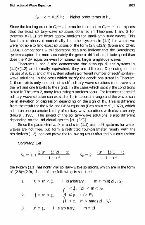
Corollary. Let

R1 5 1 11±2 ( u 2 2 1±3 )(2 l 2 1)

1 2 u 2 , R2 5 2 2( u 2 2 1±3 )(1 2 l )

1 2 u 2

the system (1.1) has nontrivial solitary-wave solutions, which are in the formof (2.8)±(2.9), if one of the following is satisfied:

1. 0 # u 2 , 1±3 , l is arbitrary, m , min{2 l , R1}

2. 1±3 , u 2 , 7±9 , 5l , 1±2 , 2 l , m , R1

l # 1±2 , m . R2

l . 1±2 , m . max {2 l , R2}

3. u 2 5 7±9 , l is arbitrary, m 5 2 l

1554 Chen

4. 7±9 , u 2 , 1, 5l , 1±2 , R1 , m , 2 l

l # 1±2 , m , R2

l . 1±2 , m , min{2 l , R2}.

We now apply Theorems 1 and 2 to some of the systems included in (1.1).

Example 1. Applying Theorem 1 to the system (1.3) (a 5 2 1±6 , b 5 c5 0, d 5 1±2 ), one recovers the exact solitary-wave solution

h (x, t) 5 27

4sech2 1 12 ! 7 1 x 1 x0 6

1

! 15t 2 2

u(x, t) 5 77

2 ! 3

5sech2 1 12 ! 7 1 x 1 x0 6

1

! 15t 2 2 (2.11)

obtained by Wang (1995) by using a homogeneous balance method.

Example 2. Let u 2 5 4±5, l 5 2 1, m 5 2 4; the resulting system is

h t 1 ux 1 (u h )x 27

30 uxxx 27

15 h xxt 5 0

ut 1 h x 1 uux 2 2±5 h xxx 2 1±2 uxxt 5 0

According to Theorem 1, this system has an exact solitary-wave solution

h (x, t) 53

8sech2 1 12 ! 5

7 1 x 1 x0 65 ! 2

6t 2 2

u (x, t) 5 61

2 ! 2sech2 1 12 ! 5

7 1 x 1 x0 65 ! 2

6t 2 2

Example 3. For the Bona±Smith system (1.10), p 5 (b 1 c)/b. Applying

Theorem 1, one finds that the solitary-wave solutions in the form of (2.8)±(2.9)

exist in the following cases:

(i) b . 0 and c . 1.(ii) b , 0, c . 0, and b 1 2c , 0.

Since

h 0 52 3(b 1 2c)

2(b 1 c)

it is easy to check that h 0 , 0 in both cases.

Combining the results in Bona et al. (1997), one can find systems which

admit exact solitary-wave solutions and also have other properties, such as

Bidirectional Wave Equation 1555

the linearized system is L2-well-posed. Recalling from results from Bona etal. (1997), one has:

Proposition. The linearized system of (1.1) is L2-well-posed if and only

if one of the following condition holds:

x a , 0, c , 0, b . 0, d . 0.

x a 5 c, b , 0, d . 0.

x b 5 d, a , 0, c . 0.

x a 5 c, b 5 d.

x a 5 0, b 5 0, c , 0, d . 0.

x c 5 0, d 5 0, a , 0, b . 0.

x a 5 2 b, c , 0, d . 0.

x a 5 2 b, d 5 2 c.

x d 5 2 c, b . 0, a , 0.

Applying the proposition to the systems in Examples 1 and 2, one finds

that the linearized system from Example 1 is not L2-well-posed, while the

linearized system from Example 2 is L2-well-posed. One might ask at thispoint which system in (1.1) should be chosen in a concrete modeling situation.

This issue is addressed by Bona and Chen (1998) and Bona et al. (1997).

The primary criteria for the choice include that the system is mathematically

well posed, preserves energy or other physical quantities conserved by the

full Euler equations, has stable solitary-wave solutions, and is suitable for

numerical simulations on a well-posed initial- and boundary-value problem.Due to the restrictions posed on the form of the exact solutions for

which we are searching, it is clear from Theorems 1 and 2 that there are

many systems which do not admit solutions of the form (2.8)±(2.9), including

the systems listed in (1.4)±(1.9). We therefore continue our search in the

next section.

3. TRAVELING-WAVE SOLUTIONS WITH u (x, t) 5 u ` 1 Asech2( l (x 1 x 0 2 Cst)

In this section, we use a more general approach to search for more exact

solutions. Denoting again j 5 x 1 x0 2 Cst, the traveling-wave solutions

(u ( j ), h ( j )) we search for in this section are the ones for which u ( j ) is of

the form u ` 1 A sech2 ( l j ), where u ` , A, and l are constants and h ( j ) tendsto h ` as j tends to 2 ` . Notice that (u ( j ), h ( j )) 5 ( a , b ) are solutions of

(1.1) for any constants a and b ; one can restrict l . 0 and search only for

nonconstant solutions. The exact solutions found in Section 2 are in this form

and can be recovered by using the method presented in this section.

1556 Chen

Starting from (2.2) and introducing functions h ( j ) 5 h ( j ) 2 h ` and

y ( j ) 5 u ( j ) 2 u ` , one obtains

2 Csh8 1 v8 1 (vh)8 1 h ` v8 1 u ` h8 1 av - 1 bCsh - 5 0(3.1)

2 Csv8 1 h8 1 vv8 1 u ` v8 1 ch - 1 dCsv - 5 0

Since h ( j ) and v ( j ) tend to zero as j tends to 2 ` , the system can be integrated

once to obtain

h ( 2 Cs 1 v 1 u ` ) 1 bCsh9 5 2 v 2 h ` v 2 av9

h 1 ch9 5 Csv 21

2v 2 2 u ` v 2 dCsv9 (3.2)

Assuming c is not zero and solving h and h9 yields

h 5 g1(v)/f (v) and h9 5 g2(v)/f (v) (3.3)

where

f (v) 5 c ( 2 Cs 1 v 1 u ` ) 2 bCs (3.4)

g1(v) 5 c ( 2 v 2 av9 2 h ` v) 2 bCs(Csv 2 1±2 v 2 2 dCsv9 2 u ` v)(3.5)

g2(v) 5 v 1 av9 1 h ` v 1 ( 2 Cs 1 v 1 u ` ) (Csv 2 1±2 v 2 2 dCsv9 2 u ` v)

Differentiating the first equation in (3.3) twice with respect to j and usingthe second equation, one obtains a fourth-order ordinary differential equation

with dependent variable v ( j ),

f 2g2 5 g 91 f 2 2 g1 f 9f 2 2g 81 ff 8 1 2g1( f 8)2

which, after substituting f, g1 and g2 into the equation, is of the form

(a1v2 1 a2v 1 a3)v + 1 (a4v 1 a5)v8v - 1 (a6v 1 a7)(v9)2

1 a8(v8)2v9 1 (a9v3 1 a10v

2 1 a11v 1 a12)v9 1 a13(v8)2 (3.6)

1 a14v5 1 a15v

4 1 a16v3 1 a17v

2 1 a18v 5 0

where ai , i 5 1, . . . , 18, depend on a, b, c, d, Cs , h ` , and u ` . With the help

of Mathematica, one sees

a1 5 bc2dC 2s 2 ac3, a2 5 2c ( 2 ac 1 bdC 2

s)( 2 (b 1 c)Cs 1 cu `

a3 5 ( 2 ac 1 bdC 2s)((b 1 c)Cs 2 cu ` )2, a4 5 2 2bc2dC 2

s 1 2ac3

a5 5 2c ( 2 ac 1 bdC 2s)((b 1 c)Cs 2 cu ` ), a6 5 a4/2

a7 5 a5 /2, a8 5 2 a4, a9 5 c 2(d 1 b /2)Cs

Bidirectional Wave Equation 1557

a10 5 2 c (3cd 1 2bd 1 3bc/2 1 3b 2/2)C 2s 2 ac2 1 3c 2 Csu ` (b /2 1 d )

a11 5 ( 2 (b 1 c)Cs 1 cu ` )( 2 2ac 2 c 2(1 1 h ` )

2 (b 2 1 2bc 1 bd 1 3cd )C 2s 1 c (2b 1 3d )Csu `

a12 5 ( 2 (b 1 c)Cs 1 cu ` )2( 2 a 2 c (1 1 h ` ) 2 (b 1 d )Cs( 2 Cs 1 u ` ))(3.7)

a13 5 ( 2 (b 1 c)Cs 1 cu ` )(2c 2(1 1 h ` ) 2 (b 2 c)bC2s 2 bcCsu ` )

a14 5 c 2/2, a15 5 2 bcCs 2 5c 2/2Cs 1 5c 2u ` /2

a16 5 2 c 2(1 1 h ` ) 1 (b 2/2 1 4bc 1 9c 2/2)C 2s

2 c (4b 1 9c)Csu ` 1 9c 2u 2` /2

a17 5 ((b 1 c)Cs 2 cu ` )(4c (1 1 h ` ) 2 (3b 1 7c)C 2s

1 (3b 1 14c)Csu ` 2 7cu2` ))/2

a18 5 ( 2 (b 1 c)Cs 1 cu ` )2( 2 1 2 h ` 1 (Cs 2 u ` )2)

We therefore established the fact that in order to find a traveling-wave

solution of (1.1), it suffices to find a solution of the ordinary differential

equation (3.6).

Theorem 3. For given a, b, c Þ 0, d, Cs , u ` , and h ` , any solution v ( j )of (3.6) will provide a traveling-wave solution u (x, t) 5 u ` 1 v ( j ), h (x, t)5 h ` 1 g1(v ( j ))/f (v ( j )), where j 5 x 1 x0 2 Cst, f, and g1 are defined in

(3.4) and (3.5). On the other hand, any traveling-wave solution ( h (x, t),u (x, t)) [ ( h ( j ), u ( j )) of system (1.1) with c Þ 0 which approaches constants

( h ` , u ` ) as j approaches 2 ` has the property that u ( j ) 2 u ` satisfies (3.6).

Instead of solving v ( j ) from (3.6) directly, which is very difficult, if

not impossible, the technique used by Kichenassamy and Olver (1992) for

a single fifth-order equation is adopted here. In the present case, the ordinary

differential equation has coefficients depending on Cs , u ` , and h ` which are

part of the unknowns. Assuming that v ( j ) can be reconstructed as the solution

of a simple first-order ordinary differential equation,

w (v) 5 (v8)2 (3.8)

once the function w ( y ) is known, y ( j ) can be solved by a simple quadrature:

#v

a

ds

! w (s)5 j 1 C (3.9)

Examples of solutions that have this form are the soliton and conoidal wave

solutions of the KDV equation (Whitham, 1974), where the function w (v)

1558 Chen

is a cubic polynomial. Solutions corresponding to w (v) in other forms can

be found in Yang et al. (1994). Using (3.8), one finds that for v8 Þ 0

(v8)2 5 w, v9 51

2w8

v8v - 51

2ww9, v + 5

1

2ww - 1

1

4w8w9 (3.10)

where the primes on w indicate derivatives with respect to v. Substituting

the above relationships into (3.6), one finds that w must satisfy a third-order

ordinary differential equation

(a1v2 1 a2v 1 a3)(

1±2 ww - 1 1±4 w8w9) 1 1±2 (a4v 1 a5)ww9

1 1±4 (a6v 1 a7)(w8)2 1 1±2 a8ww8 1 1±2 (a9v3 1 a10v

2 1 a11v 1 a12)w8 (3.11)

1 a13w 1 a14v5 1 a15v

4 1 a16v3 1 a17v

2 1 a18v 5 0

For a solitary-wave solution of the form

v ( j ) 5 A sech2( l j ), l . 0 (3.12)

the corresponding function w (v) must be a cubic polynomial:

w (v) 5 4 l 2 1 v 2 21

Av 3 2 [ r v 2 1 s v 3

where r 5 4 l 2 . 0 and s 5 2 4 l 2/A. Substituting w (v) into (3.11), the left-

hand side becomes a degree-five homogeneous polynomial in v. In order for

v to be a nontrivial solution, all the coefficients have to be zero, which yields

that r , s , Cs , u ` , and h ` have to satisfy the following algebraic equations:

a18 1 a12 r 1 a3 r 2 5 0

a17 1 (a11 1 a13) r 1 (a2 1 a5 1 a7) r 2 1 3a12s /2 1 15a3 r s /2 5 0

a16 1 a10 r 1 (a1 1 a4 1 a6 1 a8) r 2 1 (3a11/2 1 a13) s

1 (15a2/2 1 4a5 1 3a7) r s 1 15a3 s 2/2 5 0 (3.13)

a15 1 a9 r 1 3a10 s /2 1 (15a1/2 1 4a4

3a6 1 5a8/2) 1 (15a2/2 1 3a5 1 9a7/4) s 2 5 0

4a14 1 6a9 s 1 (30a1 1 12a4 1 9a6 1 6a8) s 2 5 0

which are the ultimate equations one has to solve to find solutions of the

form (3.12).

Bidirectional Wave Equation 1559

In the case that c 5 0, one sees from the second equation of (3.2) that

h 5 Csv 2 1±2 v 2 2 u ` v 2 dCsv9

Substituting h into the first equation of (3.2), one again obtains an ordinary

differential equation in v. The same technique used for (3.6) can then be used

again. We therefore can prove the following theorem.

Theorem 4. For a specified system, that is, for a given a, b, c, and d,let ai , i 5 1,. . ., 18, be as in (3.7).

(i) If c Þ 0 and ( r $ 0, s , Cs , u ` , h ` ) is a solution of (3.13), or (ii) if

c 5 0 and ( r $ 0, s , Cs , u ` , h ` ) is a solution of

(a18 1 a12 r 1 a3 r 2)/b 2 5 0

(2a17 1 2(a11 1 a13) r 1 3a12 s 1 15a3 r s )/b 2 5 0 (3.14)

(2a16 1 (3a11 1 2a13) s 1 15a3 s 2)/b 2 5 0

then system (1.1) has a traveling-wave solution which reads

u (x, t) [ u ( j ) 5 u ` 1 v ( j ) (3.15)

h (x, t) [ h ( j ) 5 H h ` 1 g1(v ( j ))/f (v ( j )), if c Þ 0

h ` 1 Csv 2 1±2 v 2 2 dCsv9 2 u ` v, if c 5 0

where v ( j ) 5 2 ( r / s )sech2(1±2 ! r j ), j 5 x 1 x0 2 Cst, and f and g1 are defined

in (3.4) and (3.5).

We now present the exact solutions found for the examples listed in the

Introduction, except for the integrable version of Boussinesq system (1.9),

which does not possess solutions in the form of (3.15). Since (3.13) and(3.14) are systems of nonlinear algebraic equations in r , s , Cs , u ` , and h ` ,

one can solve them with the help of Mathematica. The solutions we found

may only be a part of the whole set of solutions. The equalities

sech2(x)(cosh(2x) 1 1) 5 2, sech4(x)(cosh(4x) 1 4 cosh(2x) 1 3) 5 8

are used to simplifying the solutions. We will also give examples of the exact

solutions where h ` 5 0 and (or) u ` 5 0. The notation j 5 x 1 x0 2 Cst isused where x0 and Cs are real constants. When not specified, x0 and Cs are

arbitrary constants and r is a nonnegative constant.

Example 4. More exact solutions of Whitham’ s system (a 5 2 1/6, b5 0, c 5 0, d 5 1/2). Substituting a, b, c, and d into (3.14) and solving thenonlinear algebraic system, one finds

u ` 51

6Cs

1 Cs 21

2Cs r , h ` 5 2 1 1

1

36C 2s

1r12

, s 52 2

3Cs

1560 Chen

which leads to the exact solutions

u (x, t) 5 u ` 13

2Csr sech2 1 12 ! r j 2

h (x, t) 5 h ` 21

4r sech2 1 12 ! r j 2

Setting h ` 5 0 and u ` 5 0 yields C 2s 5 1/15 and r 5 7, which recovers the

exact solution (2.11) found in Example 1.

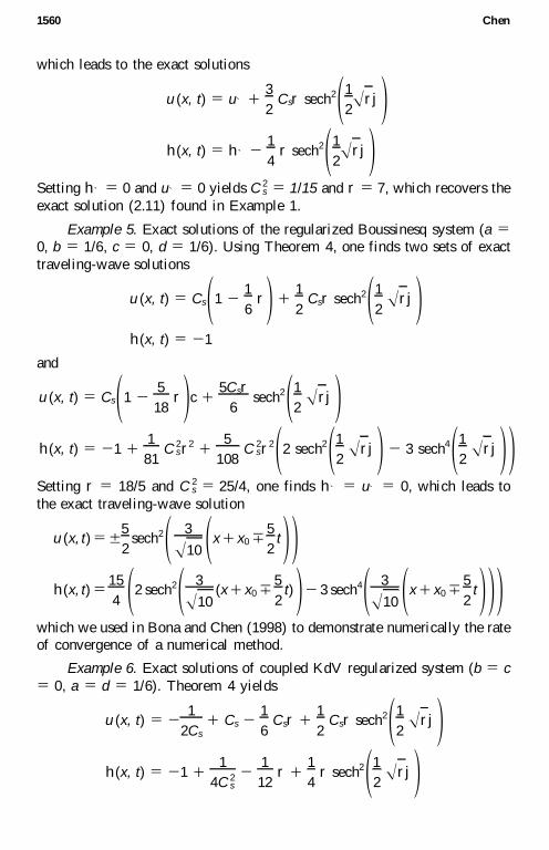
Example 5. Exact solutions of the regularized Boussinesq system (a 50, b 5 1/6, c 5 0, d 5 1/6). Using Theorem 4, one finds two sets of exact

traveling-wave solutions

u (x, t) 5 Cs 1 1 21

6r 2 1

1

2Cs r sech2 1 12 ! r j 2

h (x, t) 5 2 1

and

u (x, t) 5 Cs 1 1 25

18r 2 c 1

5Cs r6

sech2 1 12 ! r j 2h (x, t) 5 2 1 1

1

81C 2

s r 2 15

108C 2

s r 2 1 2 sech2 1 12 ! r j 2 2 3 sech4 1 12 ! r j 2 2Setting r 5 18/5 and C 2

s 5 25/4, one finds h ` 5 u ` 5 0, which leads to

the exact traveling-wave solution

u (x, t) 5 65

2sech2 1 3

! 10 1 x 1 x0 75

2t 2 2

h (x, t) 515

4 1 2 sech2 1 3

! 10(x 1 x0 7

5

2t) 2 2 3 sech4 1 3

! 10 1 x 1 x0 75

2t 2 2 2

which we used in Bona and Chen (1998) to demonstrate numerically the rateof convergence of a numerical method.

Example 6. Exact solutions of coupled KdV regularized system (b 5 c5 0, a 5 d 5 1/6). Theorem 4 yields

u (x, t) 5 21

2Cs

1 Cs 21

6Csr 1

1

2Cs r sech2 1 12 ! r j 2

h (x, t) 5 2 1 11

4C 2s

21

12r 1

1

4r sech2 1 12 ! r j 2

Bidirectional Wave Equation 1561

where setting r 5 6 and C 2s 5 1/6 gives a pair of exact traveling-wave

solutions with h ` 5 0

u (x, t) 5 7 ! 3

26 ! 3

2sech2 1 ! 3

2 1 x 1 x0 71

! 6t 2 2

h (x, t) 53

2sech2 1 ! 3

2 1 x 1 x0 71

! 6t 2 2

Example 7. Exact solutions of Boussinesq’ s original system (a 5 0, b 50, c 5 0, d 5 1/6). One can easily verify using Theorem 4 that

u (x, t) 5 1 1 21

6r 2 Cs 1

1

2Cs r sech2 1 12 ! r j 2

h (x, t) 5 2 1

are exact solutions.

Example 8. Exact solutions of coupled KdV system (a 5 1/6, b 5 0,

c 5 1/6, d 5 0). Thanks to Theorem 4 again, one finds the exact solutions

u (x, t) 5 7! 2

2 1 1 11

6r 2 1 Cs 6

1

2 ! 2r sech2 1 12 ! r j 2

h (x, t) 5 21

2 1 1 11

6r 2 1

1

4r sech2 1 12 ! r j 2

Setting r 5 6 and Cs 5 6 ! 2, one finds

u (x, t) 5 63

! 2sech2 1 ! 3

2(x 1 x0 7 ! 2t)

h (x, t) 5 2 1 13

2sech2 1 ! 3

2(x 1 x0 7 ! 2t)

Example 9. Exact solutions of coupled regularized KdV system (a 50, b 5 1/6, c 5 1/6, d 5 0). Using Theorem 4 yields the exact solutions

u (x, t) 5 Cs 1 12 21

12r 2 1

1

4Cs r sech2 1 12 ! r j 2

h (x, t) 5 2 1 1 C 2s 1 14 2

1

24r 2 1

1

8C 2

s r sech2 1 12 ! r j 2

1562 Chen

Setting r 5 6(C 2s 2 4)/C 2

s for | Cs| $ 2, one obtains

u (x, t) 51

2Cs

13

2Cs

(C 2s 2 4) sech2 1 ! 3

22

6

C 2s

j 2h (x, t) 5

3

4(C 2

s 2 4) sech2 1 ! 3

22

6

C 2s

j 2Example 10. Exact solutions to one of the Bona±Smith systems (a 5

0, b 5 d 5 1/3, c 5 2 1/3). Substituting a, b, c, and d into (3.13) and using

Theorem 4, one finds two sets of the exact solutions, which are

u (x, t) 5 1 1 21

3r 2 Cs 1 Cs r sech2 1 12 ! r j 2 (3.16)

h (x, t) 5 2 1

and

u (x, t) 51

2Cs 1 1 2

1

3r 2 1

1

2Cs r sech2 1 12 ! r j 2

h (x, t) 5 2 1 11

4C 2

s 1 1 21

3r 2 1

1

4C 2

s r sech2 1 12 ! r j 2 (3.17)

Setting r 5 3(C 2s 2 4)C 2

s for | Cs | $ 2 in (3.17), one obtains

u (x, t) 51

2Cs

13

2Cs

(C 2s 2 4) sech2 1 ! 3

2

! C 2s 2 4

Cs

j 2h (x, t) 5

3(C 2s 2 4)

4sech2 1 ! 3

2

! C 2s 2 4

Cs

j 2which recovers the exact solution found by Bona (cf. Toland, 1981).

For any system with a 5 0 and d . 0, which includes Boussinesq’ s

original system and the Bona±Smith system in Examples 7 and 10, the

following theorem provides a one-parameter family of exact traveling-

wave solutions.

Theorem 5. If a 5 0, then

u (x, t) 5 (1 2 d r )Cs 1 3dCs r sech2 1 12 ! r (x 1 x0 2 Cst) 2h (x, t) 5 2 1

are exact solutions, where x0 and Cs are arbitrary constants and r $ 0.

Bidirectional Wave Equation 1563

Proof. Substituting a 5 0 and h (x, t) 5 2 1 (i.e., h 5 0 and h ` 5 2 1)

into (3.2), the first equation is true for any u (i.e., for any v and u ` ) and the

second equation becomes after being integrated once,

(Cs 2 u ` )v 2 1±2 v 2 2 dCsv9 5 0

The same technique used for (3.6) can then be used (or applying Lemma 1

directly) to find u ` 5 (1 2 d r )Cs , and A 5 3dCs r . The theorem therefore holds.

A similar procedure can be performed to find solutions (u, h ) where his of the form h ` 1 A sech2( l j ). We will show in the next section that such

a technique will enable us to find exact solutions for the integrable version

of the Boussinesq system (1.9).

4. TRAVELING-WAVE SOLUTIONS WITH h (x, t) 5 h ` 1Asech2( l (x 1 x0 2 Cst))

Instead of searching for exact traveling-wave solutions ( h (x, t), u (x, t))where u (x, t) has the form u ` 1 A sech2( l (x 1 x0 2 Cst)), we now search

for the exact solutions where h (x, t) has the form h ` 1 A sech2( l (x 1x0 2 Cst)).

Similar to section 3, one needs first to find an ordinary differential

equation for h ( j ). In the case that a Þ 0, multiplying the first equation in

(3.2) by dCs and subtracting a times the second equation, one obtains aquadratic equation v,

2 1±2 av2 1 y (h)v 1 z(h) 5 0

where

y (h) 5 dCs(1 1 h 1 h ` ) 1 aCs 2 au `

z (h) 5 2 dC 2sh 1 dCsu ` h 1 bdC 2

sh9 2 ah 2 ach9

Denoting g (h) 5 y (h)2 1 2az(h) and solving for v, one finds

v 5y (h)

a7

1

ag (h)1/2 (4.1)

which is then substituted into (3.2) to yield

(1 1 h 1 h ` )y (h)

a2 Csh 1 u ` h 1 bCsh9 1 dCsh9

5 7 H 21

a(1 1 h 1 h ` )g (h)1/2 1

1

4g (h) 2 3/2g8(h)2 2

1

2g (h) 2 1/2g9(h) J

1564 Chen

Squaring both sides of the equation and multiplying by g (h)3 one finds a

fourth-order ordinary differential equation for h ( j ),

g (h)3 H (1 1 h 1 h ` )y (h)

a1 (u ` 2 Cs)h 1 (b 1 d )Csh9 J

2

5 H 21

a(1 1 h 1 h ` )g (h)2 1

1

4g8(h)2 2

1

2g (h)g9(h) J

2

(4.2)

where

g8(h) 5 2dCsy(h)h8 1 2a {d ( 2 Cs 1 u ` )csh8 1 bdC 2sh - 2 ah8 2 ach -

g9(h) 5 2dCsy (h)h9 1 2(dCsh8)2 1 2a {d ( 2 Cs 1 u ` )Csh9

1 bdC 2sh + 2 ah9 2 ach + }

Hence one can obtain a traveling-wave solution by solving the ordinarydifferential equation (4.2).

In the case that a 5 0, one finds from the first equation of (3.2) that

v (h) 5 2zÄ (h)

yÄ (h)

where

yÄ (h) 5 1 1 h 1 h ` , zÄ (h) 5 2 Csh 1 u ` h 1 bCsh9

Substituting v into the second equation of (3.2) and multiplying by yÄ (h)3,

one obtains again a fourth-order ordinary differential equation in h ( j ),

(Cs 2 u ` )zÄ (h)yÄ (h)2 1 (h 1 ch9)yÄ (h)3 1 1±2 zÄ (h) 2yÄ (h)

2 dC 2s (h9 1 bh + )yÄ (h)2 1 2dC 2

sh8yÄ (h)( 2 h 1 bh - ) 2 2dCszÄ (h)h9 5 0 (4.3)

The following theorem provides a relationship between the solutions of

ordinary differential equations (4.2) or (4.3) and a traveling-wave solution

of (1.1).

Theorem 6. For given (a, b, c, d, Cs , u ` , h ` ), any solution h ( j ) of (4.2)

[or (4.3) if a 5 0] will provide a traveling-wave solution h (x, t) 5 h ` 1h ( j ), u (x, t) 5 u ` 1 v ( j ), where v ( j ) is defined by (4.1) [or v ( j ) 5 2zÄ (h ( j ))/yÄ (h ( j )) if a 5 0]. On the other hand, any traveling-wave solution

( h (x, t), u (x, t)) [ ( h ( j ), u ( j )) of (1.1) which approaches constants (u ` , h ` )

as j approaches 2 ` has the property that h ( j ) 2 h ` satisfies (4.2) [or (4.3)

if a 5 0].

Bidirectional Wave Equation 1565

A similar technique can be employed to find the solution h of (4.2) [or

(4.3)] in the form of A sech2( l j ). Setting r 5 4 l 2, s 5 2 4 l 2/A, and using

formulas similar to (3.10), one finds that

(h8)2 5 r h 2 1 s h 3, h9 5 r h 13

2s h 2

h8h - 5 r 2h 2 1 4 r s h 3 1 3 s 2h 4, (4.4)

h + 5 r 2h 115

2s r h 2 1

15

2s 2h 3

Substituting these into the ordinary differential equation (4.2) [or (4.3)], one

obtains a rather complicated homogeneous polynomial equation of degree

ten (or degree five if a 5 0). For the equation to have a nontrivial solution,

all the coefficients have to be zero, which leads to a system of nonlinear

algebraic equations involving a, b, c, d, u ` , h ` , r , s , and Cs. A solution ofthe algebraic system leads to a solution of the ordinary differential equation.

Theorem 6 can then be used to find a traveling-wave solution.

Example 11. Exact solutions of the integrable version of the Boussinesq

system (b 5 c 5 d 5 0). With the procedure described above, one finds the

exact solutions

u ( j ) 5 Cs 6 ! 2 a r sech 1 12 ! r j 2if a , 0

h ( j ) 5 2 1 11

4a r 1

1

2a r sech2 1 12 ! r j 2

and

u ( j ) 5 Cs 6 ! a r tanh 1 12 ! r j ) 2if a . 0

h ( j ) 5 2 1 11

2a r sech2 1 12 ! r j 2

1566 Chen

As an example, one solution for a 5 1 (setting r 5 C 2s) is

h (x, t) 5 2 1 11

2C 2

s sech2 1 Cs

2(x 1 x0 2 Cst) 2

u (x, t) 5 Cs 1 1 6 tanh 1 Cs

2(x 1 x0 2 Cst 2 2

Remark. The system with a 5 1 has been studied using different methods.

For example, a homogeneous balance method was used in Wang (1995) and

Wang et al. (1996). In addition, a rational solution was found by Sachs (1900)using the Hirota form. For the system with a 5 1/3, a solution of the form

u ( j ) 5 A sech2 j /(1 1 B sech2 j ) was found using a Jacobi cosine elliptic

function (Krishnan, 1982).

5. CONCLUSION

In this paper we have shown that in order to find the exact traveling-

wave solutions of a given system of partial differential equations of the form

(1.1), it is sufficient to find a solution of a nonlinear fourth-order ordinary

differential equation. In consequence, any method for finding exact solutions

of ordinary differential equations can be used to generate exact traveling-

wave solutions of (1.1). For instance, one can use the Weierstrass ellipticfunction to construct periodic wave solutions (Kano and Nakayama, 1981),

inverse scattering theory to find N-soliton solutions if they exist, and use

certain ansatz equations, for instance, the ones in Yang et al. (1994), to find

traveling-wave solutions in some prescribed form.

We have found in this paper all the solutions ( h (x, t), u (x, t)) whereeither u (x, t) is of the form u ` 1 A sech2( l (x 1 x0 2 Cst)) or h (x, t) is of

the form h ` 1 A sech2( l (x 1 x0 2 Cst)) for each system listed in the

Introduction. The method presented here can also be used for the systems

h Ä t 1 (u h Ä )x 1 auxxx 2 b h Ä xxt 5 0

ut 1 h Ä x 1 uux 1 c h Ä xxx 2 duxxt 5 0,

by observing that under the transformation h Ä (x, t) 5 h (x, t) 1 1 these

systems become (1.1).

ACKNOWLEDGMENTS

This work was supported in part by NSF grants DMS-9410188 and

DMS-9622858 .

Bidirectional Wave Equation 1567

REFERENCES

Benjamin, T. B., Bona, J. L., and Mahony, J. J. (1972). Model equations for long waves in

nonlinear dispersive systems, Philosophical Transaction of the Royal London A, 272,

47±78.

Bona, J., and Chen, M. (1998). A Boussinesq system for two-way propagation of nonlinear

dispersive waves, Physica D.

Bona, J. L., Saut, J.-C., and Toland, J. F. (1997). Boussinesq equations for small-amplitude

long wavelength water waves, Preprint.

Bona, J. L., and Smith, R. (1976). A model for the two-way propagation of water waves in a

channel, Mathematical Proceedings of the Cambridge Philosophical Society, 79, 167±182.

Boussinesq, J. (1871). TheÂorie de l’ intumescence liquide appeleÂe onde solitaire ou de translation

se propageant dans un canal rectangulaire, Comptes Rendus de l’ Acadmie de Sciences,

72, 755±759.

Craig, W. (1985). An existence theory for water waves, and Boussinesq and Kortewegde Vries

scaling limits, Communication s in Partial Differential Equations, 10, 787±1003.

Fenton, J. D. (1972). A ninth-order solution for the solitary wave, Journal of Fluid Mechanics ,

53, 257±271.

Kano, K., and Nakayama, T. (1981). An exact solution of the wave equation ut 1 uux 2 uxxxxx,

Journal of the Physical Society of Japan , 50, 361±362.

Kichenassamy, S., and Olver, P. J. (1992). Existence and nonexistence of solitary wave solutions

to higher-order model evolution equations, SIAM Journal of Mathematics and Analysis,

23, 1141±1166.

Krishnan, E. V. (1982). An exact solution of the classical Boussinesq equation, Journal of the

Physical Society of Japan , 51, 2391±2392.

Newell, A. C. (1977). Finite amplitude instabilities of partial difference equations, SIAM Journal

of Applied Mathematics , 33, 133±160.

Newell, A. C. (1985). Solitons in mathematics and physics, CBMS-NSF Regional Conference

Series in Applied Mathematics, Vol 48.

Sachs, R. L. (1988). On the integrable variant of the Boussinesq system: PainleveÂproperty,

rational solutions, a related many-body system, and equivalence with AKNS hierarchy,

Physica D, 30, 1±27.

Toland, J. F. (1981). Solitary wave solutions for a model of the two-way propagation of water

waves in a channel, Mathematical Proceeding of the Cambridge Philosophical Sosiety,

90, 343±360.

Wang, Mingliang (1995). Solitary wave solutions for variant Boussinesq equations, Physics

Letters A, 199 , 169±172.

Wang, Mingliang, Yubin, Zhou, and Li, Zhibin. Application of a homogeneous balance method

to exact solutions of nonlinear equations in mathematics physics, Physics Letters A,

216 , 67±75.

Whitham, G. B. (1974). Linear and Nonlinear Waves, Wiley, New York.

Yang, Z. J., Dunlap, R. A., and Geldart, D. J. W. (1994). Exact traveling wave solutions to

nonlinear diffusion and wave equations, International Journal of Theoretical Physics,

33, 2057±2065.