Exact Matrix Completion via Convex Optimization Found Comput Math (2009) 9: 717–772 Keywords...
56
Found Comput Math (2009) 9: 717–772 DOI 10.1007/s10208-009-9045-5 Exact Matrix Completion via Convex Optimization Emmanuel J. Candès · Benjamin Recht Received: 30 May 2008 / Revised: 6 February 2009 / Accepted: 14 February 2009 / Published online: 3 April 2009 © The Author(s) 2009. This article is published with open access at Springerlink.com Abstract We consider a problem of considerable practical interest: the recovery of a data matrix from a sampling of its entries. Suppose that we observe m entries selected uniformly at random from a matrix M. Can we complete the matrix and recover the entries that we have not seen? We show that one can perfectly recover most low-rank matrices from what appears to be an incomplete set of entries. We prove that if the number m of sampled entries obeys m ≥ Cn 1.2 r log n for some positive numerical constant C, then with very high probability, most n × n matrices of rank r can be perfectly recovered by solving a simple convex optimization program. This program finds the matrix with minimum nuclear norm that fits the data. The condition above assumes that the rank is not too large. However, if one replaces the 1.2 exponent with 1.25, then the result holds for all values of the rank. Similar results hold for arbitrary rectangular matrices as well. Our results are connected with the recent literature on compressed sensing, and show that objects other than signals and images can be perfectly reconstructed from very limited information. Communicated by Michael Todd. E.J. Candès ( ) Applied and Computational Mathematics, Caltech, Pasadena, CA 91125, USA e-mail: [email protected] B. Recht Center for the Mathematics of Information, Caltech, Pasadena, CA 91125, USA e-mail: [email protected]
Transcript of Exact Matrix Completion via Convex Optimization Found Comput Math (2009) 9: 717–772 Keywords...
Found Comput Math (2009) 9: 717–772DOI 10.1007/s10208-009-9045-5
Exact Matrix Completion via Convex Optimization
Emmanuel J. Candès · Benjamin Recht
Received: 30 May 2008 / Revised: 6 February 2009 / Accepted: 14 February 2009 /Published online: 3 April 2009© The Author(s) 2009. This article is published with open access at Springerlink.com
Abstract We consider a problem of considerable practical interest: the recovery of adata matrix from a sampling of its entries. Suppose that we observe m entries selecteduniformly at random from a matrix M . Can we complete the matrix and recover theentries that we have not seen?
We show that one can perfectly recover most low-rank matrices from what appearsto be an incomplete set of entries. We prove that if the number m of sampled entriesobeys
m ≥ C n1.2r logn
for some positive numerical constant C, then with very high probability, most n × n
matrices of rank r can be perfectly recovered by solving a simple convex optimizationprogram. This program finds the matrix with minimum nuclear norm that fits the data.The condition above assumes that the rank is not too large. However, if one replacesthe 1.2 exponent with 1.25, then the result holds for all values of the rank. Similarresults hold for arbitrary rectangular matrices as well. Our results are connected withthe recent literature on compressed sensing, and show that objects other than signalsand images can be perfectly reconstructed from very limited information.
Communicated by Michael Todd.
E.J. Candès (�)Applied and Computational Mathematics, Caltech, Pasadena, CA 91125, USAe-mail: [email protected]
B. RechtCenter for the Mathematics of Information, Caltech, Pasadena, CA 91125, USAe-mail: [email protected]

718 Found Comput Math (2009) 9: 717–772
Keywords Matrix completion · Low-rank matrices · Convex optimization · Dualityin optimization · Nuclear norm minimization · Random matrices · NoncommutativeKhintchine inequality · Decoupling · Compressed sensing
Mathematics Subject Classification (2000) Primary 90C25 · Secondary 90C59 ·15A52
1 Introduction
In many practical problems of interest, one would like to recover a matrix from asampling of its entries. As a motivating example, consider the task of inferring an-swers in a partially filled out survey. That is, suppose that questions are being askedto a collection of individuals. Then we can form a matrix where the rows index eachindividual and the columns index the questions. We collect data to fill out this tablebut unfortunately, many questions are left unanswered. Is it possible to make an ed-ucated guess about what the missing answers should be? How can one make such aguess? Formally, we may view this problem as follows. We are interested in recover-ing a data matrix M with n1 rows and n2 columns, but only get to observe a numberm of its entries which is comparably much smaller than n1n2, the total number ofentries. Can one recover the matrix M from m of its entries? In general, everyonewould agree that this is impossible without some additional information.
In many instances, however, the matrix we wish to recover is known to be struc-tured in the sense that it is low-rank or approximately low-rank. (We recall for com-pleteness that a matrix with n1 rows and n2 columns has rank r if its rows or columnsspan an r-dimensional space.) Below are two examples of practical scenarios whereone would like to be able to recover a low-rank matrix from a sampling of its entries.
• The Netflix problem. In the area of recommender systems, users submit ratings ona subset of entries in a database, and the vendor provides recommendations basedon the user’s preferences [30, 34]. Because users only rate a few items, one wouldlike to infer their preference for unrated items.
A special instance of this problem is the now famous Netflix problem [1]. Users(rows of the data matrix) are given the opportunity to rate movies (columns of thedata matrix), but users typically rate only very few movies so that there are very fewscattered observed entries of this data matrix. Yet, one would like to complete thismatrix so that the vendor (here Netflix) might recommend titles that any particularuser is likely to be willing to order. In this case, the data matrix of all user-ratingsmay be approximately low-rank because it is commonly believed that only a fewfactors contribute to an individual’s tastes or preferences.
• Triangulation from incomplete data. Suppose we are given partial informationabout the distances between objects and would like to reconstruct the low-dimensional geometry describing their locations. For example, we may have anetwork of low-power wirelessly networked sensors scattered randomly across aregion. Suppose each sensor only has the ability to construct distance estimatesbased on signal strength readings from its nearest fellow sensors. From these noisydistance estimates, we can form a partially observed distance matrix. We can then

Found Comput Math (2009) 9: 717–772 719
estimate the true distance matrix whose rank will be equal to two if the sensors arelocated in a plane or three if they are located in three dimensional space [25, 33].In this case, we only need to observe a few distances per node to have enoughinformation to reconstruct the positions of the objects.
These examples are, of course, far from exhaustive and there are many other problemswhich fall in this general category. For instance, we may have some very limitedinformation about a covariance matrix of interest. Yet, this covariance matrix maybe low-rank or approximately low-rank because the variables only depend upon acomparably smaller number of factors.
1.1 Impediments and Solutions
Suppose for simplicity that we wish to recover a square n × n matrix M of rank r .1
Such a matrix M can be represented by n2 numbers, but it only has (2n− r)r degreesof freedom. This fact can be revealed by counting parameters in the singular valuedecomposition (the number of degrees of freedom associated with the description ofthe singular values and of the left and right singular vectors). When the rank is small,this is considerably smaller than n2. For instance, when M encodes a 10-dimensionalphenomenon, then the number of degrees of freedom is about 20n offering a reduc-tion in dimensionality by a factor about equal to n/20. When n is large (e.g., in thethousands or millions), the data matrix carries much less information than its ambientdimension suggests. The problem is now whether it is possible to recover this matrixfrom a sampling of its entries without having to probe all the n2 entries, or moregenerally collect n2 or more measurements about M .
1.1.1 Which Matrices?
In general, one cannot hope to be able to recover a low-rank matrix from a sample ofits entries. Consider the rank-1 matrix M equal to
M = e1e∗n =
⎡⎢⎢⎢⎣
0 0 · · · 0 10 0 · · · 0 0...
......
......
0 0 · · · 0 0
⎤⎥⎥⎥⎦ , (1.1)
where here and throughout, ei is the ith canonical basis vector in Euclidean space(the vector with all entries equal to 0 but the ith equal to 1). This matrix has a 1in the top-right corner and all the other entries are 0. Clearly, this matrix cannot berecovered from a sampling of its entries unless we pretty much see all the entries.The reason is that for most sampling sets, we would only get to see zeros so that wewould have no way of guessing that the matrix is not zero. For instance, if we were
1We emphasize that there is nothing special about M being square and all of our discussion would applyto arbitrary rectangular matrices as well. The advantage of focusing on square matrices is a simplifiedexposition and reduction in the number of parameters of which we need to keep track.
720 Found Comput Math (2009) 9: 717–772
to see 90% of the entries selected at random, then 10% of the time we would only getto see zeroes.
It is therefore impossible to recover all low-rank matrices from a set of sampled en-tries but can one recover most of them? To investigate this issue, we introduce a sim-ple model of low-rank matrices. Consider the singular value decomposition (SVD) ofa matrix M
M =r∑
k=1
σkukv∗k, (1.2)
where the uk’s and vk’s are the left and right singular vectors, and the σk’s are the sin-gular values (the roots of the eigenvalues of M∗M). Then we could think of a genericlow-rank matrix as follows: the families {uk}1≤k≤r and {vk}1≤k≤r are sampled uni-formly at random among all families of r orthonormal vectors independently of eachother. (The independence between these two families simplifies the exposition, and isnot crucial.) We make no assumptions about the singular values σk . In the sequel, wewill refer to this model as the random orthogonal model. This model is convenient inthe sense that it is both very concrete and simple, and useful in the sense that it willhelp us fix the main ideas. In the sequel, however, we will consider far more generalmodels. The question for now is whether or not one can recover such a generic matrixfrom a sampling of its entries.
1.1.2 Which Sampling Sets?
Clearly, one cannot hope to reconstruct any low-rank matrix M—even of rank 1—ifthe sampling set avoids any column or row of M . Suppose that M is of rank 1 and ofthe form xy∗, x,y ∈ R
n so that the (i, j)th entry is given by
Mij = xiyj .
Then if we do not have samples from the first row, for example, one could never guessthe value of the first component of x1 by any method whatsoever; no informationabout x1 is observed. There is of course nothing special about the first row and thisargument extends to any row or column. To have any hope of recovering an unknownmatrix, one needs at least one observation per row and one observation per column.
We have just seen that if the sampling is adversarial, e.g., one observes all of theentries of M but those in the first row, then one would not even be able to recovermatrices of rank 1. But what happens for most sampling sets? Can one recover alow-rank matrix from almost all sampling sets of cardinality m? Formally, supposethat the set � of locations corresponding to the observed entries ((i, j) ∈ � if Mij
is observed) is a set of cardinality m sampled uniformly at random. Then can onerecover a generic low-rank matrix M , perhaps with very large probability, from theknowledge of the value of its entries in the set �?
1.1.3 Which Algorithm?
If the number of measurements is sufficiently large, and if the entries are sufficientlyuniformly distributed as above, one might hope that there is only one low-rank matrix

Found Comput Math (2009) 9: 717–772 721
with these entries. If this were true, one would want to recover the data matrix bysolving the optimization problem
minimize rank(X)
subject to Xij = Mij (i, j) ∈ �,(1.3)
where X is the decision variable and rank(X) is equal to the rank of the matrix X.The program (1.3) is a common sense approach which simply seeks the simplestexplanation fitting the observed data. If there were only one low-rank object fitting thedata, this would recover M . This is unfortunately of little practical use because thisoptimization problem is not only NP-hard, but all known algorithms which provideexact solutions require time doubly exponential in the dimension n of the matrix inboth theory and practice [13].
If a matrix has rank r , then it has exactly r nonzero singular values so that the rankfunction in (1.3) is simply the number of nonvanishing singular values. In this paper,we consider an alternative which minimizes the sum of the singular values over theconstraint set. This sum is called the nuclear norm,
‖X‖∗ =n∑
k=1
σk(X) (1.4)
where, here and below, σk(X) denotes the kth largest singular value of X. The heuris-tic optimization is then given by
minimize ‖X‖∗subject to Xij = Mij (i, j) ∈ �.
(1.5)
Whereas the rank function counts the number of nonvanishing singular values, thenuclear norm sums their amplitude and in some sense, is to the rank functional whatthe convex �1 norm is to the counting �0 norm in the area of sparse signal recovery.The main point here is that the nuclear norm is a convex function and, as we willdiscuss in Sect. 1.4 can be optimized efficiently via semidefinite programming.
1.1.4 A First Typical Result
Our first result shows that, perhaps unexpectedly, this heuristic optimization recoversa generic M when the number of randomly sampled entries is large enough. We willprove the following theorem.
Theorem 1.1 Let M be an n1 × n2 matrix of rank r sampled from the random or-thogonal model, and put n = max(n1, n2). Suppose we observe m entries of M withlocations sampled uniformly at random. Then there are numerical constants C and c
such that if
m ≥ C n5/4r logn , (1.6)
the minimizer to the problem (1.5) is unique and equal to M with probability at least1−cn−3 logn; that is to say, the semidefinite program (1.5) recovers all the entries of

722 Found Comput Math (2009) 9: 717–772
M with no error. In addition, if r ≤ n1/5, then the recovery is exact with probabilityat least 1 − cn−3 logn provided that
m ≥ C n6/5r logn. (1.7)
Furthermore, (1.7) holds even when the two families of singular vectors are depen-dent; all that is needed is that the marginal distribution of each family is uniform.
The theorem states that a surprisingly small number of entries are sufficient tocomplete a generic low-rank matrix. For small values of the rank, e.g., when r = O(1)
or r = O(logn), one only needs to see on the order of n6/5 entries (ignoring logarith-mic factors) which is considerably smaller than n2—the total number of entries of asquare matrix. The real feat, however, is that the recovery algorithm is tractable andvery concrete. Hence, the contribution is twofold:
• Under the hypotheses of Theorem 1.1, there is a unique low-rank matrix which isconsistent with the observed entries.
• Further, this matrix can be recovered by the convex optimization (1.5). In otherwords, for most problems, the nuclear norm relaxation is formally equivalent tothe combinatorially hard rank minimization problem (1.3).
Theorem 1.1 is in fact a special instance of a far more general theorem that covers amuch larger set of matrices M . We describe this general class of matrices and preciserecovery conditions in the next section.
1.2 Main Results
As seen in our first example (1.1), it is impossible to recover a matrix which is equalto zero in nearly all of its entries unless we see all the entries of the matrix. To recovera low-rank matrix, this matrix cannot be in the null space of the “sampling operator”that provides the values of a subset of the entries. Now, it is easy to see that if thesingular vectors of a matrix M are highly concentrated, then M could very well be inthe null-space of the sampling operator. For instance, consider the rank-2 symmetricmatrix M given by
M =2∑
k=1
σkuku∗k, u1 = (e1 + e2)/
√2, u2 = (e1 − e2)/
√2,
where the singular values are arbitrary. Then this matrix vanishes everywhere exceptin the top-left 2 × 2 corner and one would basically need to see all the entries ofM to be able to recover this matrix exactly by any method whatsoever. There is anendless list of examples of this sort. Hence, we arrive at the notion that somehow thesingular vectors need to be sufficiently spread—that is, uncorrelated with the standardbasis—in order to minimize the number of observations needed to recover a low-rankmatrix.2 This motivates the following definition.
2Both the left and right singular vectors need to be uncorrelated with the standard basis. Indeed, the matrixe1v∗ has its first row equal to v and all the others equal to zero. Clearly, this rank-1 matrix cannot berecovered unless we basically see all of its entries.
Found Comput Math (2009) 9: 717–772 723
Definition 1.2 Let U be a subspace of Rn of dimension r and P U be the orthogonal
projection onto U . Then the coherence of U (vis-à-vis the standard basis (ei )) isdefined to be
μ(U) ≡ n
rmax
1≤i≤n‖P Uei‖2. (1.8)
Note that for any subspace, the smallest μ(U) can be is 1, achieved, for example,if U is spanned by vectors whose entries all have magnitude 1/
√n. The largest pos-
sible value for μ(U) is n/r which would correspond to any subspace that contains astandard basis element. We shall be primarily interested in subspaces with low coher-ence as matrices whose column and row spaces have low coherence cannot really bein the null space of the sampling operator. For instance, we will see that the randomsubspaces discussed above have nearly minimal coherence.
To state our main result, we introduce two assumptions about an n1 × n2 matrixM whose SVD is given by M =∑
1≤k≤r σkukv∗k and with column and row spaces
denoted by U and V, respectively.
A0 The coherences obey max(μ(U),μ(V )) ≤ μ0 for some positive μ0.A1 The n1 ×n2 matrix
∑1≤k≤rukv
∗k has a maximum entry bounded by μ1
√r/(n1n2)
in absolute value for some positive μ1.
The μ’s above may depend on r and n1, n2. Moreover, note that A1 always holdswith μ1 = μ0
√r since the (i, j)th entry of the matrix
∑1≤k≤r ukv
∗k is given by∑
1≤k≤r uikvjk and by the Cauchy–Schwarz inequality,
∣∣∣∣∑
1≤k≤r
uikvjk
∣∣∣∣≤√ ∑
1≤k≤r
|uik|2√ ∑
1≤k≤r
|vjk|2 ≤ μ0r√n1n2
.
Hence, for sufficiently small ranks, μ1 is comparable to μ0. As we will see in Sect. 2,for larger ranks, both subspaces selected from the uniform distribution and spacesconstructed as the span of singular vectors with bounded entries are not only incoher-ent with the standard basis, but also obey A1 with high probability for values of μ1
at most logarithmic in n1 and/or n2. Below, we will assume that μ1 is greater than orequal to 1.
We are in the position to state our main result: if a matrix has row and columnspaces that are incoherent with the standard basis, then nuclear norm minimizationcan recover this matrix from a random sampling of a small number of entries.
Theorem 1.3 Let M be an n1 ×n2 matrix of rank r obeying A0 and A1 and put n =max(n1, n2). Suppose we observe m entries of M with locations sampled uniformlyat random. Then there exist constants C, c such that if
m ≥ C max(μ2
1,μ1/20 μ1,μ0n
1/4)nr(β logn) (1.9)
for some β > 2, then the minimizer to the problem (1.5) is unique and equal to M
with probability at least 1 − cn−β . For r ≤ μ−10 n1/5 and under A0 only, this estimate
724 Found Comput Math (2009) 9: 717–772
can be improved to
m ≥ C μ0 n6/5r(β logn) (1.10)
with the same probability of success.
Theorem 1.3 asserts that if the coherence is low, few samples are required to re-cover M . For example, if μ0 = O(1) and the rank is not too large, then the recoveryis exact with large probability provided that
m ≥ C n6/5r logn. (1.11)
We emphasize that if one is interested in low-rank matrices, there is only one as-sumption: A0. Below, we give two illustrative examples of matrices with incoherentcolumn and row spaces. This list is by no means exhaustive.
1. The first example is the random orthogonal model. For values of the rank r greaterthan logn, μ(U) and μ(V ) are O(1), μ1 = O(logn) both with very large proba-bility. Hence, the recovery is exact provided that m obeys (1.6) or (1.7). Special-izing Theorem 1.3 to these values of the parameters gives Theorem 1.1. Hence,Theorem 1.1 is a special case of our general recovery result.
2. The second example is more general and, in a nutshell, simply requires that thecomponents of the singular vectors of M are small. Assume that the uj and vj ’sobey
maxij
∣∣〈ei ,uj 〉∣∣2 ≤ μB/n, max
ij
∣∣〈ei ,vj 〉∣∣2 ≤ μB/n, (1.12)
for some value of μB = O(1). Then the maximum coherence is at most μB sinceμ(U) ≤ μB and μ(V ) ≤ μB . Further, we will see in Sect. 2 that A1 holds most ofthe time with μ1 = O(
√logn). Thus, for matrices with singular vectors obeying
(1.12), the recovery is exact provided that m obeys (1.11) for values of the ranknot exceeding μ−1
B n1/5.
1.3 Extensions
Our main result (Theorem 1.3) extends to a variety of other low-rank matrix comple-tion problems beyond the sampling of entries. Indeed, suppose we have two ortho-normal bases f 1, . . . ,f n and g1, . . . ,gn of R
n, and that we are interested in solvingthe rank minimization problem
minimize rank(X)
subject to f ∗i Xgj = f ∗
i Mgj , (i, j) ∈ �.(1.13)
To see that our theorem provides conditions under which (1.13) can be solved vianuclear norm minimization, note that there exist unitary transformations F and G
such that ej = Ff j and ej = Ggj for each j = 1, . . . , n. Hence,
f ∗i Xgj = e∗
i
(FXG∗)ej .

Found Comput Math (2009) 9: 717–772 725
Then if the conditions of Theorem 1.3 hold for the matrix FXG∗, it is immediate thatnuclear norm minimization finds the unique optimal solution of (1.13) when we areprovided a large enough random collection of the inner products f ∗
i Mgj . In otherwords, all that is needed is that the column and row spaces of M be respectivelyincoherent with the basis (f i ) and (gi ).
From this perspective, we additionally remark that our results likely extend to thecase where one observes a small number of arbitrary linear functionals of a hiddenmatrix M . Set N = n2 and let A1, . . . ,AN be an orthonormal basis for the linearspace of n × n matrices with the usual inner product 〈X,Y 〉 = trace(X∗Y ). Then weexpect our results should also apply to the rank minimization problem
minimize rank(X)
subject to 〈Ak,X〉 = 〈Ak,M〉 k ∈ �,(1.14)
where � ⊂ {1, . . . ,N} is selected uniformly at random. In fact, (1.14) is (1.3) whenthe orthobasis is the canonical basis (eie
∗j )1≤i,j≤n. Here, those low-rank matrices
which have small inner product with all the basis elements Ak may be recoverable bynuclear norm minimization. To avoid unnecessary confusion and notational clutter,we leave this general low-rank recovery problem for future work.
1.4 Connections, Alternatives and Prior Art
Nuclear norm minimization is a recent heuristic introduced by Fazel in [19], and is anextension of the trace heuristic often used by the control community; see, e.g., [4, 28].Indeed, when the matrix variable is symmetric and positive semidefinite, the nuclearnorm of X is the sum of the (nonnegative) eigenvalues and thus equal to the traceof X. Hence, for positive semidefinite unknowns, (1.5) would simply minimize thetrace over the constraint set:
minimize trace(X)
subject to Xij = Mij (i, j) ∈ �,
X � 0.
This is a semidefinite program. Even for the general matrix M which may not bepositive definite or even symmetric, the nuclear norm heuristic can be formulated interms of semidefinite programming as, for instance, the program (1.5) is equivalentto
minimize trace(W 1) + trace(W 2)
subject to Xij = Mij (i, j) ∈ �,[W 1 X
X∗ W 2
]� 0
with optimization variables X, W 1 and W 2, (see, e.g., [19, 37]). There are manyefficient algorithms and high-quality software available for solving these types ofproblems.
Our work is inspired by results in the emerging field of compressive sampling orcompressed sensing, a new paradigm for acquiring information about objects of inter-est from what appears to be a highly incomplete set of measurements [10, 12, 16]. In

726 Found Comput Math (2009) 9: 717–772
practice, this means for example that high-resolution imaging is possible with fewersensors, or that one can speed up signal acquisition time in biomedical applicationsby orders of magnitude, simply by taking far fewer specially coded samples. Math-ematically speaking, we wish to reconstruct a signal x ∈ R
n from a small numbermeasurements y = Φx, y ∈ R
m, and m is much smaller than n; i.e., we have farfewer equations than unknowns. In general, one cannot hope to reconstruct x, butassume now that the object we wish to recover is known to be structured in the sensethat it is sparse (or approximately sparse). This means that the unknown object de-pends upon a smaller number of unknown parameters. Then it has been shown that �1minimization allows recovery of sparse signals from remarkably few measurements:supposing Φ is chosen randomly from a suitable distribution, then with very highprobability, all sparse signals with about k nonzero entries can be recovered from onthe order of k logn measurements. For instance, if x is k-sparse in the Fourier do-main, i.e., x is a superposition of k sinusoids, then it can be perfectly recovered withhigh probability—by �1 minimization—from the knowledge of about k logn of itsentries sampled uniformly at random [10].
From this viewpoint, the results in this paper greatly extend the theory of com-pressed sensing by showing that other types of interesting objects or structures, be-yond sparse signals and images, can be recovered from a limited set of measure-ments. Moreover, the techniques for proving our main results build upon ideas fromthe compressed sensing literature together with probabilistic tools such as the power-ful techniques of Bourgain and of Rudelson for bounding norms of operators betweenBanach spaces.
Our notion of incoherence generalizes the concept of the same name in compres-sive sampling. Notably, in [9], the authors introduce the notion of the incoherence ofa unitary transformation. Letting U be an n × n unitary matrix, the coherence of Uis given by
μ(U) = nmaxj,k
|Ujk|2.
This quantity ranges in values from 1 for a unitary transformation whose entriesall have the same magnitude to n for the identity matrix. Using this notion, [9]showed that with high probability, a k-sparse signal could be recovered via lin-ear programming from the observation of the inner product of the signal withm = �(μ(U)k logn) randomly selected columns of the matrix U . This result pro-vided a generalization of the celebrated results about partial Fourier observationsdescribed in [10], a special case where μ(U) = 1. This paper generalizes the notionof incoherence to problems beyond the setting of sparse signal recovery.
In [29], the authors studied the nuclear norm heuristic applied to a related problemwhere partial information about a matrix M is available from m equations of the form
⟨A(k),M
⟩=∑ij
A(k)ij Mij = bk, k = 1, . . . ,m, (1.15)
where for each k, {A(k)ij } is an i.i.d. sequence of Gaussian or Bernoulli random vari-
ables and the sequences {A(k)} are also independent from each other (the sequences{A(k)} and {bk} are available to the analyst). Building on the concept of restricted

Found Comput Math (2009) 9: 717–772 727
isometry introduced in [11] in the context of sparse signal recovery, [29] establishesthe first sufficient conditions for which the nuclear norm heuristic returns the mini-mum rank element in the constraint set. They prove that the heuristic succeeds withlarge probability whenever the number m of available measurements is greater thana constant times 2nr logn for n × n matrices. Although this is an interesting result, aserious impediment to this approach is that one needs to essentially measure randomprojections of the unknown data matrix—a situation which unfortunately does notcommonly arise in practice. Further, the measurements in (1.15) give some informa-tion about all the entries of M whereas in our problem, information about most ofthe entries is simply not available. In particular, the results and techniques introducedin [29] do not begin to address the matrix completion problem of interest to us in thispaper. As a consequence, our methods are completely different; for example, theydo not rely on any notions of restricted isometry. Instead, as we discuss below, weprove the existence of a Lagrange multiplier for the optimization (1.5) that certifiesthe unique optimal solution is precisely the matrix that we wish to recover.
We would like to note that other recovery algorithms may be possible when thesampling happens to be chosen in a very special fashion. For example, suppose thatM is generic and that we precisely observe every entry in the first r rows and columnsof the matrix. Write M in block form as
M =[M11 M12M21 M22
]
with M11 an r × r matrix. In the special case that M11 is invertible and M hasrank r , then it is easy to verify that M22 = M21M
−111 M12. One can prove this iden-
tity by forming the SVD of M , for example. That is, if M is generic, and the upperr × r block is invertible, and we observe every entry in the first r rows and columns,we can recover M . This result immediately generalizes to the case where one ob-serves precisely r rows and r columns and the r × r matrix at the intersection of theobserved rows and columns is invertible. However, this scheme has many practicaldrawbacks that stand in the way of a generalization to a completion algorithm from ageneral set of entries. First, if we miss any entry in these rows or columns, we cannotrecover M , nor can we leverage any information provided by entries of M22. Second,if the matrix has rank less than r , and we observe r rows and columns, a combina-torial search to find the collection that has an invertible square subblock is required.Several authors have observed that if the set of rows and columns is selected at ran-dom, then this rank deficiency is highly improbable. For example, [17, 18] show thatif the columns are sampled from a distribution proportional to the column Euclideannorms of the matrix, then a low rank matrix can be reconstructed with no error. Again,even after randomization, this method does not work when some of the entries in thesampled columns are missing. Moreover, in the setting considered in this paper, thereis no oracle that would inform us about the norm of a row or column.
Finally, we note that in [3] the authors propose to solve a version of the matrixcompletion problem where the provided entries are corrupted by noise. They computethe SVD of the matrix which is equal to Mij when (i, j) ∈ � and zeros everywhereelse. They show that when the underlying matrix M has rank r , this procedure resultsin a rank-r approximation which constructs most entries of M to error o(1) as long as
728 Found Comput Math (2009) 9: 717–772
the noise is small. Unfortunately, this procedure is not useful in the context where theentries are not noisy: the bound provides a reconstruction error which scales as O(n)
in the Frobenius norm. This is in sharp contrast to our algorithm which reconstructsthe matrix with no error as long as � has sufficiently large cardinality.
1.5 Notations and Organization of the Paper
The paper is organized as follows. We first argue in Sect. 2 that the random orthogo-nal model and, more generally, matrices with incoherent column and row spaces obeythe assumptions of the general Theorem 1.3. To prove Theorem 1.3, we first establishsufficient conditions which guarantee that the true low-rank matrix M is the uniquesolution to (1.5) in Sect. 3. One of these conditions is the existence of a dual vectorobeying two crucial properties. Section 4 constructs such a dual vector and providesthe overall architecture of the proof which shows that, indeed, this vector obeys thedesired properties provided that the number of measurements is sufficiently large.Surprisingly, as explored in Sect. 5, the existence of a dual vector certifying that M
is unique is related to some problems in random graph theory including “the couponcollector’s problem.” Following this discussion, we prove our main result via severalintermediate results which are all proven in Sect. 6. Section 7 introduces numericalexperiments showing that matrix completion based on nuclear norm minimizationworks well in practice. Section 8 closes the paper with a short summary of our find-ings, a discussion of important extensions and improvements. In particular, we willdiscuss possible ways of improving the 1.2 exponent in (1.10) so that it gets closerto 1. Finally, the Appendix provides proofs of auxiliary lemmas supporting our mainargument.
Before continuing, we provide here a brief summary of the notations used through-out the paper. Matrices are bold capital, vectors are bold lowercase and scalars or en-tries are not bold. For instance, X is a matrix and Xij its (i, j)th entry. Likewise x isa vector and xi its ith component. When we have a collection of vectors uk ∈ R
n for1 ≤ k ≤ d , we will denote by uik the ith component of the vector uk and [u1, . . . ,ud ]will denote the n × d matrix whose kth column is uk .
A variety of norms on matrices will be discussed. The spectral norm of a matrixis denoted by ‖X‖. The Euclidean inner product between two matrices is 〈X,Y 〉 =trace(X∗Y ), and the corresponding Euclidean norm, called the Frobenius or Hilbert–Schmidt norm, is denoted ‖X‖F . That is, ‖X‖F = 〈X,X〉1/2. The nuclear norm of amatrix X is ‖X‖∗. For q ≥ 1, the Schatten q-norm of a matrix is denoted by
‖X‖Sq =(
n∑i=1
σi(X)q
)1/q
. (1.16)
Note that the nuclear, Frobenius, and operator norms are respectively equal to theSchatten 1-, 2- and ∞-norms. The maximum entry of X (in absolute value) is denotedby ‖X‖∞ ≡ maxij |Xij |. For vectors, we will only consider the usual Euclidean �2norm, which we simply write as ‖x‖.
Further, we will also manipulate linear transformations which act on matri-ces and will use calligraphic letters for these operators as in A(X). In particular,

Found Comput Math (2009) 9: 717–772 729
the identity operator will be denoted by I . The only norm we will consider forthese operators is their spectral norm (the top singular value) denoted by ‖A‖ =supX:‖X‖F ≤1 ‖A(X)‖F .
Finally, we adopt the convention that C denotes a numerical constant indepen-dent of the matrix dimensions, rank, and number of measurements, whose value maychange from line to line. Certain special constants with precise numerical values willbe ornamented with subscripts (e.g., CR). Any exceptions to this notational schemewill be noted in the text.
2 Which Matrices Are Incoherent?
In this section, we restrict our attention to square n × n matrices, but the extension torectangular n1 × n2 matrices immediately follows by setting n = max(n1, n2).
2.1 Incoherent Bases Span Incoherent Subspaces
Almost all n × n matrices M with singular vectors {uk}1≤k≤r and {vk}1≤k≤r whosecomponents have magnitude bounded by μB as in (1.12) also satisfy the assump-tions A0 and A1 with μ0 = μB , μ1 = CμB
√logn for some positive constant C. As
mentioned above, A0 holds automatically, but observe that A1 would not hold with asmall value of μ1 if the matrices [u1, . . . ,ur ] and [v1, . . . ,vr ] have a row in commonwhere all of the entries have magnitude
√μB/n. It is not hard to see that in this case
∥∥∥∥∑
k
ukv∗k
∥∥∥∥∞= μB r/n.
Certainly, this example is constructed in a very special way, and should occur infre-quently. We now show that it is generically unlikely.
Consider the matrixr∑
k=1
εkukv∗k, (2.1)
where {εk}1≤k≤r is an arbitrary sign sequence. For almost all choices of sign se-quences, A1 is satisfied with μ1 = O(μB
√logn). Indeed, if one selects the signs
uniformly at random, then for each β > 0,
P
(∥∥∥∥∥r∑
k=1
εkukvk
∥∥∥∥∥∞≥ μB
√8βr logn/n
)≤ (
2n2)n−β. (2.2)
This is of interest because suppose the low-rank matrix we wish to recover is of theform
M =r∑
k=1
λkukv∗k (2.3)

730 Found Comput Math (2009) 9: 717–772
with scalars λk . Since the vectors {uk} and {vk} are orthogonal, the singular valuesof M are given by |λk| and the singular vectors are given by sgn(λk)uk and vk fork = 1, . . . , r . Hence, in this model, A1 concerns the maximum entry of the matrixgiven by (2.1) with εk = sgn(λk). That is to say, for most sign patterns, the matrix ofinterest obeys an appropriate size condition. We emphasize here that the only thingthat we assumed about the uk’s and vk’s was that they had small entries. In particular,they could be equal to each other as would be the case for a symmetric matrix.
The claim (2.2) is a simple application of Hoeffding’s inequality. The (i, j)th entryof (2.1) is given by
Zij =∑
1≤k≤r
εkuikvjk,
and is a sum of r zero-mean independent random variables, each bounded by μB/n.Therefore,
P(|Zij | ≥ λμB
√r/n
)≤ 2e−λ2/8.
Setting λ proportional to√
logn and applying the union bound gives the claim.To summarize, we say that M is sampled from the incoherent basis model if it is
of the form
M =r∑
k=1
εkσkukv∗k; (2.4)
{εk}1≤k≤r is a random sign sequence, and {uk}1≤k≤r and {vk}1≤k≤r have maximumentries of size at most
√μB/n.
Lemma 2.1 There exist numerical constants c and C such that for any β > 0,matrices from the incoherent basis model obey the assumption A1 with μ1 ≤CμB
√(β + 2) logn with probability at least 1 − cn−β .
2.2 Random Subspaces Are Incoherent
In this section, we prove that the random orthogonal model obeys the two assump-tions A0 and A1 (with appropriate values for the μ’s) with large probability.
Lemma 2.2 Set r̄ = max(r, logn). Then there exist constants C and c such that therandom orthogonal model obeys:3
1. maxi ‖P Uei‖2 ≤ C r̄/n
2. ‖∑1≤k≤r ukv∗k‖∞ ≤ C logn
√r̄/n
with probability 1 − cn−3 logn. The second estimate assumes independence betweenthe families {uk}1≤k≤r and {vk}1≤k≤r .
3When r ≥ C′(logn)3 for some positive constant C′, a better estimate is possible, namely,‖∑1≤k≤r ukv∗
k‖∞ ≤ C
√r logn/n.

Found Comput Math (2009) 9: 717–772 731
We note that an argument similar to the following proof would give that if C is ofthe form Kβ where K is a fixed numerical constant, we can achieve a probability atleast 1 − cn−β provided that n is sufficiently large. To establish these facts, we makeuse of the standard result below [22].
Lemma 2.3 Let Yd be distributed as a chi-squared random variable with d degreesof freedom. Then for each t > 0
P(Yd − d ≥ t
√2d + t2)≤ e−t2/2 and P
(Yd − d ≤ −t
√2d)≤ e−t2/2. (2.5)
We will use (2.5) as follows: for each ε ∈ (0,1), we have
P(Yd ≥ d (1 − ε)−1)≤ e−ε2d/4 and P
(Yd ≤ d (1 − ε)
)≤ e−ε2d/4. (2.6)
We begin with the first assertion of Lemma 2.2. Observe that it follows from
‖P Uei‖2 =∑
1≤k≤r
u2ik, (2.7)
that Zr ≡ ‖P Uei‖2 (for fixed i) is the squared Euclidean length of the first r com-ponents of a unit vector uniformly distributed on the unit sphere in n dimensions.Now, suppose that x1, x2, . . . , xn are i.i.d. N(0,1). Then the distribution of a unitvector uniformly distributed on the sphere is that of x/‖x‖ and, therefore, the lawof Zr is that of Yr/Yn, where Yr = ∑
k≤r x2k . Fix ε > 0 and consider the event
An,ε = {Yn/n ≥ 1 − ε}. For each λ > 0, it follows from (2.6) that
P(Zr − r/n ≥ λ
√2r/n
)= P(Yr ≥ [
r + λ√
2r]Yn/n
)
≤ P(Yr ≥ [
r + λ√
2r]Yn/n and An,ε
)+ P(Ac
n,ε
)
≤ P(Yr ≥ [
r + λ√
2r][1 − ε])+ e−ε2n/4
= P(Yr − r ≥ λ
√2r[1 − ε − ε
√r/2λ2
])+ e−ε2n/4.
Now pick ε = 4(n−1 logn)1/2, λ = 8√
2 logn and assume that n is sufficiently largeso that
ε(
1 +√
r/2λ2)
≤ 1/2.
Then
P(Zr − r/n ≥ λ
√2r/n
)≤ P(Yr − r ≥ (λ/2)
√2r)+ n−4.
Assume now that r ≥ 4 logn (which means that λ ≤ 4√
2r). Then it follows from(2.5) that
P(Yr − r ≥ (λ/2)
√2r)≤ P
(Yr − r ≥ (λ/4)
√2r + (λ/4)2)≤ e−λ2/32 = n−4.

732 Found Comput Math (2009) 9: 717–772
Hence,
P(Zr − r/n ≥ 16
√r logn/n
)≤ 2n−4
and, therefore,
P
(max
i‖P Uei‖2 − r/n ≥ 16
√r logn/n
)≤ 2n−3 (2.8)
by the union bound. Note that (2.8) establishes the first claim of the lemma (even forr < 4 logn since in this case Zr ≤ Z�4 logn�).
It remains to establish the second claim. Notice that by symmetry, E =∑1≤k≤r ukv
∗k has the same distribution as
F =r∑
k=1
εkukv∗k,
where {εk} is an independent Rademacher sequence.4 It then follows from Hoeffd-ing’s inequality that conditional on {uk} and {vk} we have
P(|Fij | > t
)≤ 2e−t2/2σ 2
ij , σ 2ij =
∑1≤k≤r
u2ikv
2ik.
As shown below, maxij |vij |2 ≤ (10 logn)/n with large probability, and thus
σ 2ij ≤ 10
logn
n‖P Uei‖2.
Set r̄ = max(r, logn). Since ‖P Uei‖2 ≤ Cr̄/n with large probability, we have
σ 2ij ≤ C(logn) r̄/n2
with large probability. Hence, the marginal distribution of Fij obeys
P(|Fij | > λ
√r̄/n
)≤ 2e−γ λ2/ logn + P(σ 2
ij ≥ C(logn)r̄/n2).
for some numerical constant γ . Picking λ = γ ′ logn where γ ′ is a sufficiently largenumerical constant gives
‖F‖∞ ≤ C (logn)√
r̄/n
with large probability. Since E and F have the same distribution, the second claimfollows. More sophisticated arguments would provide small improvements but wechoose not to pursue these refinements here.
4A Rademacher sequence is a (possibly infinite) sequence of independent random variables taking thevalues 1 and −1 with equal probability.
Found Comput Math (2009) 9: 717–772 733
The claim about the size of maxij |vij |2 is straightforward since our techniquesshow that for each λ > 0
P(Z1 ≥ λ(logn)/n
)≤ P(Y1 ≥ λ(1 − ε) logn
)+ e−ε2n/4.
Moreover,
P(Y1 ≥ λ(1 − ε) logn
)= P(|x1| ≥
√λ(1 − ε) logn
)≤ 2e− 12 λ(1−ε) logn.
If n is sufficiently large so that ε ≤ 1/5, this gives P(Z1 ≥ 10(logn)/n) ≤ 3n−4 and,therefore,
P
(max
ij|vij |2 ≥ 10(logn)/n
)≤ 12n−3 logn
since the maximum is taken over at most 4n logn pairs.
3 Duality
Let R� : Rn1×n2 → R
|�| be the sampling operator which extracts the observed en-tries, R�(X) = (Xij )ij∈�, so that the constraint in (1.5) becomes R�(X) = R�(M).Standard convex optimization theory asserts that X is a solution to (1.5) if there existsa dual vector (or Lagrange multiplier) λ ∈ R
|�| such that R∗� λ is a subgradient of
the nuclear norm at the point X, which we denote by
R∗� λ ∈ ∂‖X‖∗ (3.1)
(see, e.g., [5]). Recall the definition of a subgradient of a convex function f :R
n1×n2 → R. We say that Y is a subgradient of f at X0, denoted Y ∈ ∂f (X0), if
f (X) ≥ f (X0) + 〈Y ,X − X0〉 (3.2)
for all X.Suppose X0 ∈ R
n1×n2 has rank r with a singular value decomposition given by
X0 =∑
1≤k≤r
σk ukv∗k. (3.3)
With these notations, Y is a subgradient of the nuclear norm at X0 if and only if it isof the form
Y =∑
1≤k≤r
ukv∗k + W , (3.4)
where W obeys the following two properties:
(i) The column space of W is orthogonal to U ≡ span (u1, . . . ,ur ), and the rowspace of W is orthogonal to V ≡ span (v1, . . . ,vr ).
(ii) The spectral norm of W is less than or equal to 1.
734 Found Comput Math (2009) 9: 717–772
(see, e.g., [24, 38]). To express these properties concisely, it is convenient to introducethe orthogonal decomposition R
n1×n2 = T ⊕T ⊥ where T is the linear space spannedby elements of the form ukx
∗ and yv∗k , 1 ≤ k ≤ r , where x and y are arbitrary, and
T ⊥ is its orthogonal complement. Note that dim(T ) = r(n1 + n2 − r), precisely thenumber of degrees of freedom in the set of n1 × n2 matrices of rank r . T ⊥ is thesubspace of matrices spanned by the family (xy∗), where x (respectively y) is anyvector orthogonal to U (respectively V ).
The orthogonal projection PT onto T is given by
PT (X) = P UX + XP V − P UXP V , (3.5)
where P U and P V are the orthogonal projections onto U and V . Note here that whileP U and P V are matrices, PT is a linear operator mapping matrices to matrices. Wealso have
PT ⊥(X) = (I − PT )(X) = (In1 − P U)X(In2 − P V )
where I d denotes the d × d identity matrix. With these notations, Y ∈ ∂‖X0‖∗ if
(i′) PT (Y ) =∑1≤k≤r ukv
∗k , and
(ii′) ‖PT ⊥Y‖ ≤ 1.
Now that we have characterized the subgradient of the nuclear norm, the lemmabelow gives sufficient conditions for the uniqueness of the minimizer to (1.5).
Lemma 3.1 Consider a matrix X0 =∑rk=1 σk ukv
∗k of rank r which is feasible for
the problem (1.5), and suppose that the following two conditions hold:
1. There exists a dual point λ such that Y = R∗�λ obeys
PT (Y ) =r∑
k=1
ukv∗k,
∥∥PT ⊥(Y )∥∥< 1. (3.6)
2. The sampling operator R� restricted to elements in T is injective.
Then X0 is the unique minimizer.
Before proving this result, we would like to emphasize that this lemma pro-vides a clear strategy for proving our main result, namely Theorem 1.3. LettingM = ∑r
k=1 σk ukv∗k , M is the unique solution to (1.5) if the injectivity condition
holds and if one can find a dual point λ such that Y = R∗�λ obeys (3.6).
The proof of Lemma 3.1 uses a standard fact which states that the nuclear normand the spectral norm are dual to one another.
Lemma 3.2 For each pair W and H , we have
〈W ,H 〉 ≤ ‖W‖‖H‖∗.
In addition, for each H , there is a W obeying ‖W‖ = 1 which achieves the equality.

Found Comput Math (2009) 9: 717–772 735
A variety of proofs are available for this lemma, and an elementary argument issketched in [29]. We now turn to the proof of Lemma 3.1.
Proof of Lemma 3.1 Consider any perturbation X0 + H where R�(H ) = 0. Thenfor any W 0 obeying (i)–(ii),
∑rk=1 ukv
∗k + W 0 is a subgradient of the nuclear norm
at X0 and, therefore,
‖X0 + H‖∗ ≥ ‖X0‖∗ +⟨
r∑k=1
ukv∗k + W 0,H
⟩.
Letting W = PT ⊥(Y ), we may write∑r
k=1 ukv∗k = R∗
�λ − W . Since ‖W‖ < 1 andR�(H ) = 0, it then follows that
‖X0 + H‖∗ ≥ ‖X0‖∗ + ⟨W 0 − W ,H
⟩.
Now, by construction,
⟨W 0 − W ,H
⟩= ⟨PT ⊥
(W 0 − W
),H
⟩= ⟨W 0 − W , PT ⊥(H )
⟩.
We use Lemma 3.2 and set W 0 = PT ⊥(Z) where Z is any matrix obeying ‖Z‖ ≤ 1and 〈Z, PT ⊥(H )〉 = ‖PT ⊥(H )‖∗. Then W 0 ∈ T ⊥, ‖W 0‖ ≤ 1, and
⟨W 0 − W ,H
⟩≥ (1 − ‖W‖)∥∥PT ⊥(H )
∥∥∗,
which by assumption is strictly positive unless PT ⊥(H ) = 0. In other words, ‖X0 +H‖∗ > ‖X0‖∗ unless PT ⊥(H ) = 0. Assume then that PT ⊥(H ) = 0 or equivalentlythat H ∈ T . Then R�(H ) = 0 implies that H = 0 by the injectivity assumption. Inconclusion, ‖X0 + H‖∗ > ‖X0‖∗ unless H = 0. �
4 Architecture of the Proof
Our strategy to prove that M =∑1≤k≤r σkukv
∗k is the unique minimizer to (1.5) is to
construct a matrix Y which vanishes on �c and obeys the conditions of Lemma 3.1(and show the injectivity of the sampling operator restricted to matrices in T alongthe way). Set P� to be the orthogonal projector onto the indices in � so that the(i, j)th component of P�(X) is equal to Xij if (i, j) ∈ � and zero otherwise. Ourcandidate Y will be the solution to
minimize ‖X‖F
subject to (PT P�)(X) =r∑
k=1
ukv∗k.
(4.1)
The matrix Y vanishes on �c as otherwise it would not be an optimal solution sinceP�(Y ) would obey the constraint and have a smaller Frobenius norm. Hence, Y =
736 Found Comput Math (2009) 9: 717–772
P�(Y ) and PT (Y ) =∑rk=1 ukv
∗k . Since the Pythagoras formula gives
‖Y‖2F = ∥∥PT (Y )
∥∥2F
+ ∥∥PT ⊥(Y )∥∥2
F=∥∥∥∥∥
r∑k=1
ukv∗k
∥∥∥∥∥2
F
+ ∥∥PT ⊥(Y )∥∥2
F
= r + ∥∥PT ⊥(Y )∥∥2
F,
minimizing the Frobenius norm of X amounts to minimizing the Frobenius norm ofPT ⊥(X) under the constraint PT (X) =∑r
k=1 ukv∗k . Our motivation is twofold. First,
the solution to the least-squares problem (4.1) has a closed form that is amenable toanalysis. Second, by forcing PT ⊥(Y ) to be small in the Frobenius norm, we hopethat it will be small in the spectral norm as well, and establishing that ‖PT ⊥(Y )‖ < 1would prove that M is the unique solution to (1.5).
To compute the solution to (4.1), we introduce the operator A�T defined by
A�T (M) = P�PT (M).
Then if A∗�T A�T = PT P�PT has full rank when restricted to T , the minimizer to
(4.1) is given by
Y = A�T
(A∗
�T A�T
)−1(E), E ≡
r∑k=1
ukv∗k. (4.2)
We clarify the meaning of (4.2) to avoid any confusion. (A∗�T A�T )−1(E) is meant
to be that element F in T obeying (A∗�T A�T )(F ) = E.
To summarize the aims of our proof strategy,
• We must first show that A∗�T A�T = PT P�PT is a one-to-one linear mapping
from T onto itself. In this case, A�T = P�PT —as a mapping from T to Rn1×n2 —
is injective. This is the second sufficient condition of Lemma 3.1. Moreover, ouransatz for Y given by (4.2) is well defined.
• Having established that Y is well defined, we will show that
∥∥PT ⊥(Y )∥∥< 1,
thus proving the first sufficient condition.
4.1 The Bernoulli Model
Instead of showing that the theorem holds when � is a set of size m sampled uni-formly at random, we prove the theorem for a subset �′ sampled according to theBernoulli model. Here and below, {δij }1≤i≤n1,1≤j≤n2 is a sequence of independentidentically distributed 0/1 Bernoulli random variables with
P(δij = 1) = p ≡ m
n1n2, (4.3)

Found Comput Math (2009) 9: 717–772 737
and define
�′ = {(i, j) : δij = 1
}. (4.4)
Note that E |�′| = m, so that the average cardinality of �′ is that of �. Then follow-ing the same reasoning as the argument developed in Sect. II.C of [10] shows thatthe probability of “failure” under the uniform model is bounded by 2 times the prob-ability of failure under the Bernoulli model; the failure event is the event on whichthe solution to (1.5) is not exact. Hence, we can restrict our attention to the Bernoullimodel and from now on, we will assume that � is given by (4.4). This is advanta-geous because the Bernoulli model admits a simpler analysis than uniform samplingthanks to the independence between the δij ’s.
4.2 The Injectivity Property
We study the injectivity of A�T , which also shows that Y is well defined. To provethis, we will show that the linear operator p−1 PT (P� − pI)PT has small operatornorm, which we recall is sup‖X‖F ≤1 p−1‖PT (P� − pI)PT (X)‖F .
Theorem 4.1 Suppose � is sampled according to the Bernoulli model (4.3)–(4.4)and put n = max(n1, n2). Suppose that the coherences obey max(μ(U),μ(V )) ≤ μ0.Then there is a numerical constant CR such that for all β > 1,
p−1 ‖PT P�PT − pPT ‖ ≤ CR
√μ0 nr(β logn)
m(4.5)
with probability at least 1 − 3n−β provided that CR
√μ0 nr(β logn)
m< 1.
Proof Decompose any matrix X as X =∑ab〈X, eae
∗b〉eae
∗b so that
PT (X) =∑ab
⟨PT (X), eae
∗b
⟩eae
∗b =
∑ab
⟨X, PT
(eae
∗b
)⟩eae
∗b.
Hence, P�PT (X) =∑ab δab 〈X, PT (eae
∗b)〉 eae
∗b which gives
(PT P�PT )(X) =∑ab
δab
⟨X, PT
(eae
∗b
)⟩PT
(eae
∗b
).
In other words,
PT P�PT =∑ab
δab PT
(eae
∗b
)⊗ PT
(eae
∗b
),
where x ⊗ y, in which x and y belong to some Hilbert space H , is the outer productdefined as (x ⊗ y)(z) = x〈y,z〉H . It follows from the definition (3.5) of PT that
PT
(eae
∗b
)= (P Uea)e∗b + ea(P V eb)
∗ − (P Uea)(P V eb)∗. (4.6)
738 Found Comput Math (2009) 9: 717–772
This gives
∥∥PT
(eae
∗b
)∥∥2F
= ⟨PT
(eae
∗b
), eae
∗b
⟩= ‖P Uea‖2 + ‖P V eb‖2 − ‖P Uea‖2 ‖P V eb‖2
(4.7)and since ‖P Uea‖2 ≤ μ(U)r/n1 and ‖P V eb‖2 ≤ μ(V )r/n2,
∥∥PT
(eae
∗b
)∥∥2F
≤ 2μ0r/min(n1, n2). (4.8)
Now, the fact that the operator PT P�PT does not deviate from its expected value
E(PT P�PT ) = PT (E P�)PT = PT (pI)PT = pPT
in the spectral norm is related to Rudelson’s selection theorem [31]. The first part ofthe theorem below may be found in [9], for example, see also [32] for a very similarstatement.
Theorem 4.2 [9] Let {δab} be independent 0/1 Bernoulli variables with P(δab =1)=p = m
n1n2and put n = max(n1, n2). Suppose that ‖PT (eae
∗b)‖2
F ≤ 2μ0r/n. Set
Z ≡ p−1∥∥∥∥∑ab
(δab − p) PT
(eae
∗b
)⊗ PT
(eae
∗b
)∥∥∥∥= p−1‖PT P�PT − pPT ‖.
1. There exists a constant C′R such that
EZ ≤ C′R
√μ0 nr logn
m(4.9)
provided that the right-hand side is smaller than 1.2. Suppose EZ ≤ 1. Then for each λ > 0, we have
P
(|Z − EZ| > λ
√μ0 nr logn
m
)
≤ 3 exp
(−γ ′
0 min
{λ2 logn,λ
√m logn
μ0 nr
})(4.10)
for some positive constant γ ′0.
As mentioned above, the first part, namely (4.9) is an application of an establishedresult which states that if {yi} is a family of vectors in R
d and {δi} is a 0/1 Bernoullisequence with P(δi = 1) = p, then
p−1∥∥∥∥∑
i
(δi − p)yi ⊗ yi
∥∥∥∥≤ C
√logd
pmax
i‖yi‖
Found Comput Math (2009) 9: 717–772 739
for some C > 0 provided that the right-hand side is less than 1. The proof may befound in the cited literature, e.g., in [9]. Hence, the first part follows from apply-ing this result to matrices of the form PT (eae
∗b) and using the available bound on
‖PT (eae∗b)‖F . The second part follows from Talagrand’s concentration inequality
and may be found in the Appendix.
Set λ =√
β/γ ′0 and assume that m > (β/γ ′
0)μ0 nr logn. Then the left-hand side
of (4.10) is bounded by 3n−β, and thus we established that
Z ≤ C′R
√μ0 nr logn
m+ 1√
γ ′0
√μ0 nr β logn
m
with probability at least 1 − 3n−β . Setting CR = C′R + 1/
√γ ′
0 finishes the proof. �
Take m large enough so that CR
√μ0 (nr/m) logn ≤ 1/2. Then it follows from
(4.5) that
p
2
∥∥PT (X)∥∥
F≤ ∥∥(PT P�PT )(X)
∥∥F
≤ 3p
2
∥∥PT (X)∥∥
F(4.11)
for all X with large probability. In particular, the operator A∗�T A�T = PT P�PT
mapping T onto itself is well conditioned, and hence invertible. An immediate con-sequence is the following corollary.
Corollary 4.3 Assume that CR
√μ0nr(logn)/m ≤ 1/2. With the same probability
as in Theorem 4.1, we have∥∥P�PT (X)
∥∥F
≤√3p/2
∥∥PT (X)∥∥
F. (4.12)
Proof We have ‖P�PT (X)‖2F = 〈X, (P�PT )∗(P�PT )X〉 = 〈X, (PT P�PT )X〉,
and thus∥∥P�PT (X)
∥∥2F
= ⟨PT (X), (PT P�PT )(X)
⟩≤ ∥∥PT (X)∥∥
F
∥∥(PT P�PT )(X)∥∥
F,
where the inequality is due to Cauchy–Schwarz. The conclusion (4.12) followsfrom (4.11). �
4.3 The Size Property
In this section, we explain how we will show that ‖PT ⊥(Y )‖ < 1. This result willfollow from five lemmas that we will prove in Sect. 6. Introduce
H ≡ PT − p−1 PT P�PT ,
which obeys ‖H(X)‖F ≤ CR
√μ0(nr/m)β logn‖PT (X)‖F with large probability
because of Theorem 4.1. For any matrix X ∈ T , (PT P�PT )−1(X) can be expressedin terms of the power series
(PT P�PT )−1(X) = p−1(X + H(X) + H2(X) + · · · )

740 Found Comput Math (2009) 9: 717–772
for H is a contraction when m is sufficiently large. Since Y = P�PT (PT P�PT )−1 ×(∑
1≤k≤r ukv∗k), PT ⊥(Y ) may be decomposed as
PT ⊥(Y ) = p−1(PT ⊥ P�PT )(E + H(E) + H2(E) + · · · ), E =
∑1≤k≤r
ukv∗k.
(4.13)To bound the norm of the left-hand side, it is of course sufficient to bound the normof the summands in the right-hand side. Taking the following five lemmas togetherestablishes Theorem 1.3.
Lemma 4.4 Fix β ≥ 2 and λ ≥ 1. There is a numerical constant C0 such that ifm ≥ λμ2
1 nrβ logn, then
p−1∥∥(PT ⊥ P�PT )E
∥∥≤ C0 λ−1/2 (4.14)
with probability at least 1 − n−β .
Lemma 4.5 Fix β ≥ 2 and λ ≥ 1. There are numerical constants C1 and c1 such thatif m ≥ λμ1 max(
√μ0,μ1) nrβ logn, then
p−1∥∥(PT ⊥ P�PT )H(E)
∥∥≤ C1 λ−1 (4.15)
with probability at least 1 − c1n−β .
Lemma 4.6 Fix β ≥ 2 and λ ≥ 1. There are numerical constants C2 and c2 such thatif m ≥ λμ
4/30 nr4/3β logn, then
p−1∥∥(PT ⊥ P�PT )H2(E)
∥∥≤ C2 λ−3/2 (4.16)
with probability at least 1 − c2n−β .
Lemma 4.7 Fix β ≥ 2 and λ ≥ 1. There are numerical constants C3 and c3 such thatif m ≥ λμ2
0 nr2β logn, then
p−1∥∥(PT ⊥ P�PT )H3(E)
∥∥≤ C3 λ−1/2 (4.17)
with probability at least 1 − c3n−β .
Lemma 4.8 Under the assumptions of Theorem 4.1, there is a numerical constantCk0 such that if m ≥ (2CR)2μ0nrβ logn, then
p−1∥∥∥∥(PT ⊥ P�PT )
∑k≥k0
Hk(E)
∥∥∥∥≤ Ck0
(n2r
m
)1/2(μ0nrβ logn
m
)k0/2
(4.18)
with probability at least 1 − 3n−β .
Found Comput Math (2009) 9: 717–772 741
Let us now show how we may combine these lemmas to prove our main results.Under all of the assumptions of Theorem 1.3, consider the four Lemmas 4.4, 4.5, 4.6,and 4.8, the latter applied with k0 = 3. Together they imply that there are numeri-cal constants c and C such that ‖PT ⊥(Y )‖ < 1 with probability at least 1 − cn−β
provided that the number of samples obeys
m ≥ C max(μ2
1,μ1/20 μ1,μ
4/30 r1/3,μ0n
1/4)nrβ logn (4.19)
for some constant C. The four expressions in the maximum come from Lemmas 4.4,4.5, 4.6, and 4.8 in this order. Now, the bound (4.19) is only interesting in the rangewhen μ0n
1/4r is smaller than a constant times n as otherwise the right-hand sideis greater than n2 (this would say that one would see all the entries in which caseour claim is trivial). When μ0r ≤ n3/4, (μ0r)
4/3 ≤ μ0n5/4r, and thus the recovery is
exact provided that m obeys (1.9).For the case concerning small values of the rank, we consider all five lemmas
and apply Lemma 4.8, the latter applied with k0 = 4. Together they imply that‖PT ⊥(Y )‖ < 1 with probability at least 1 − cn−β provided that the number of sam-ples obeys
m ≥ C max(μ2
0r,μ0n1/5)nrβ logn (4.20)
for some constant C. The two expressions in the maximum come from Lemmas 4.7and 4.8 in this order. The reason for this simplified formulation is that the terms μ2
1,
μ1/20 μ1 and μ
4/30 r1/3 which come from Lemmas 4.4, 4.5, and 4.6 are bounded above
by μ20r since μ1 ≤ μ0
√r . When μ0r ≤ n1/5, the recovery is exact provided that m
obeys (1.10).
5 Connections with Random Graph Theory
5.1 The Injectivity Property and the Coupon Collector’s Problem
We argued in the Introduction that to have any hope of recovering an unknown matrixof rank 1 by any method whatsoever, one needs at least one observation per row andone observation per column. Sample m entries uniformly at random. Viewing therow indices as bins, assign the kth sampled entry to the bin corresponding to itsrow index. Then to have any hope of recovering our matrix, all the bins need to beoccupied. Quantifying how many samples are required to fill all of the bins is thefamous coupon collector’s problem.
Coupon collection is also connected to the injectivity of the sampling operator P�
restricted to elements in T . Suppose we sample the entries of a rank 1 matrix equalto xy∗ with left and right singular vectors u = x/‖x‖ and v = y/‖y‖, respectively,and have not seen anything in the ith row. Then we claim that P� (restricted to T )has a nontrivial null space, and thus PT P�PT is not invertible. Indeed, consider thematrix eiv
∗. This matrix is in T and
P�
(eiv
∗)= 0
742 Found Comput Math (2009) 9: 717–772
since eiv∗ vanishes outside of the ith row. The same applies to the columns as well.
If we have not seen anything in column j , then the rank-1 matrix ue∗j ∈ T and
P�(ue∗j ) = 0. In conclusion, the invertibility of PT P�PT implies a complete col-
lection.When the entries are sampled uniformly at random, it is well known that one
needs on the order of n logn samples to sample all the rows. What is interesting isthat Theorem 4.1 implies that PT P�PT is invertible—a stronger property—whenthe number of samples is also on the order of n logn. A particular implication of thisdiscussion is that the logarithmic factors in Theorem 4.1 are unavoidable.
5.2 The Injectivity Property and the Connectivity Problem
To recover a matrix of rank 1, one needs much more than at least one observationper row and column. Let R be the set of row indices, 1 ≤ i ≤ n, and C be the set ofcolumn indices, 1 ≤ j ≤ n, and consider the bipartite graph connecting vertices i ∈ R
to vertices j ∈ C if and only if (i, j) ∈ �, i.e., the (i, j)th entry is observed. We claimthat if this graph is not fully connected, then one cannot hope to recover a matrix ofrank 1.
To see this, we let I be the set of row indices and J be the set of column indices inany connected component. We will assume that I and J are nonempty as otherwise,one is in the previously discussed situation where some rows or columns are notsampled. Consider a rank 1 matrix equal to xy∗ as before with singular vectors u =x/‖x‖ and v = y/‖y‖. Then all the information about the values of the xi ’s withi ∈ I and of the yj ’s with j ∈ J are given by the sampled entries connecting I toJ since all the other observed entries connect vertices in I c to those in J c. Noweven if one observes all the entries xiyj with i ∈ I and j ∈ J , then at least the signsof xi , i ∈ I , and of yj , j ∈ J , would remain undetermined. Indeed, if the values(xi)i∈I , (yj )j∈J are consistent with the observed entries, so are the values (−xi)i∈I ,(−yj )j∈J . However, since the same analysis holds for the sets I c and J c , there are atleast two matrices consistent with the observed entries and exact matrix completionis impossible.
The connectivity of the graph is also related to the injectivity of the samplingoperator P� restricted to elements in T . If the graph is not fully connected, then weclaim that P� (restricted to T ) has a nontrivial null space, and thus PT P�PT is notinvertible. Indeed, consider the matrix
M = av∗ + ub∗,
where ai = −ui if i ∈ I and ai = ui otherwise, and bj = vj if j ∈ J and bj = −vj
otherwise. Then this matrix is in T and obeys
Mij = 0
if (i, j) ∈ I × J or (i, j) ∈ I c × J c . Note that on the complement, i.e., (i, j) ∈ I × J c
or (i, j) ∈ I c ×J , one has Mij = 2uivj and one can show that M �= 0 unless uv∗ = 0.Since � is included in the union of I × J and I c × J c , we have that P�(M) = 0. Inconclusion, the invertibility of PT P�PT implies a fully connected graph.

Found Comput Math (2009) 9: 717–772 743
When the entries are sampled uniformly at random, it is well known that one needson the order of n logn samples to obtain a fully connected graph with large probabil-ity (see, e.g., [6]). Remarkably, Theorem 4.1 implies that PT P�PT is invertible—astronger property—when the number of samples is also on the order of n logn.
6 Proofs of the Critical Lemmas
In this section, we prove the five lemmas of Sect. 4.3. Before we begin, however, wedevelop a simple estimate which we will use throughout. For each pair (a, b) and(a′, b′), it follows from the expression of PT (eae
∗b) (4.6) that
⟨PT
(ea′e∗
b′), eae
∗b
⟩ = 〈ea,P Uea′ 〉1{b=b′} + 〈eb,P V eb′ 〉1{a=a′}− 〈ea,P Uea′ 〉〈eb,P V eb′ 〉. (6.1)
Fix μ0 obeying μ(U) ≤ μ0 and μ(V ) ≤ μ0 and note that∣∣〈ea,P Uea′ 〉∣∣= ∣∣〈P Uea,P Uea′ 〉∣∣≤ ‖P Uea‖‖P Uea′ ‖ ≤ μ0r/n1
and similarly for 〈eb,P V eb′ 〉. Suppose that b = b′ and a �= a′, then∣∣⟨PT
(ea′e∗
b′), eae
∗b
⟩∣∣= ∣∣〈ea,P Uea′ 〉∣∣(1 − ‖P V eb‖2)≤ μ0r/n1.
We have a similar bound when a = a′ and b �= b′ whereas when a �= a′ and b �= b′,∣∣⟨PT
(ea′e∗
b′), eae
∗b
⟩∣∣≤ (μ0r)2/(n1n2).
In short, it follows from this analysis (and from (4.8) for the case where (a, b) =(a′, b′)) that
maxab,a′b′
∣∣⟨PT
(ea′e∗
b′), eae
∗b
⟩∣∣≤ 2μ0r/min(n1, n2). (6.2)
A consequence of (4.8) is the estimate:∑a′b′
∣∣⟨PT
(ea′e∗
b′), eae
∗b
⟩∣∣2 =∑a′b′
∣∣⟨PT
(eae
∗b
), ea′e∗
b′⟩∣∣2
= ∥∥PT
(eae
∗b
)∥∥2F
≤ 2μ0r/min(n1, n2), (6.3)
which we will apply several times. A related estimate is this:
maxa
∑b
|Eab|2 ≤ μ0r/min(n1, n2), (6.4)
and the same is true by exchanging the role of a and b. To see this, write
∑b
|Eab|2 = ∥∥e∗aE∥∥2 =
∥∥∥∥∑j≤r
vj 〈uj , ea〉∥∥∥∥
2
=∑j≤r
∣∣〈uj , ea〉∣∣2 = ‖P Uea‖2,
and the conclusion follows from the coherence property.

744 Found Comput Math (2009) 9: 717–772
We will prove the lemmas in the case where n1 = n2 = n for simplicity, i.e., inthe case of square matrices of dimension n. The general case is treated in exactly thesame way. In fact, the argument only makes use of the bounds (6.2), (6.3), and (6.4),and the general case is obtained by replacing n with min(n1, n2).
Each of the following subsections computes the operator norm of some randomvariable. In each section, we denote S as the quantity whose norm we wish to analyze.We will also frequently use the notation H for some auxiliary matrix variable whosenorm we will need to bound. Hence, we will reuse the same notation many timesrather than introducing a dozen new names—just as in computer programming whereone uses the same variable name in distinct routines.
6.1 Proof of Lemma 4.4
In this section, we develop a bound on
p−1∥∥PT ⊥ P�PT (E)
∥∥= p−1∥∥PT ⊥(P� − pI)PT (E)
∥∥≤ p−1
∥∥(P� − pI)(E)∥∥,
where the equality follows from PT ⊥ PT = 0, and the inequality from PT (E) = Etogether with ‖PT ⊥(X)‖ ≤ ‖X‖ which is valid for any matrix X. Set
S ≡ p−1(P� − pI)(E) = p−1∑ab
(δab − p)Eabeae∗b. (6.5)
We think of S as a random variable since it depends on the random δab’s, and notethat ES = 0.
The proof of Lemma 4.4 operates by developing an estimate on the size of(E‖S‖q)1/q for some q ≥ 1 and by applying Markov inequality to bound the tail ofthe random variable ‖S‖. To do this, we shall use a symmetrization argument and thenoncommutative Khintchine inequality. Since the function f (S) = ‖S‖q is convex,Jensen’s inequality gives that
E‖S‖q ≤ E∥∥S − S′∥∥q
,
where S′ = p−1∑ab(δ
′ab −p)Eabeae
∗b is an independent copy of S. Since (δab −δ′
ab)
is symmetric, S − S′ has the same distribution as
p−1∑ab
εab
(δab − δ′
ab
)Eabeae
∗b ≡ Sε − S′
ε,
where {εab} is an independent Rademacher sequence and Sε = p−1∑ab εabδabEab ×
eae∗b . Further, the triangle inequality gives
(E∥∥Sε − S′
ε
∥∥q)1/q ≤ (E‖Sε‖q
)1/q + (E∥∥S′
ε
∥∥q)1/q = 2(E‖Sε‖q
)1/q
since Sε and S′ε have the same distribution and, therefore,
(E‖S‖q
)1/q ≤ 2p−1(
Eδ Eε
∥∥∥∥∑ab
εabδab Eabeae∗b
∥∥∥∥q)1/q
.

Found Comput Math (2009) 9: 717–772 745
We are now in position to apply the noncommutative Khintchine inequality whichbounds the Schatten norm of a Rademacher series. Recall from Sect. 1.5 that forq ≥ 1, the Schatten q-norm of a matrix is the quantity (1.16). The following theo-rem was originally proven by Lust–Picquard [26], and was later sharpened by Buch-holz [7].
Lemma 6.1 (Noncommutative Khintchine inequality) Let (Xi )1≤i≤r be a finite se-quence of matrices of the same dimension and let {εi} be a Rademacher sequence.For each q ≥ 2,
[Eε
∥∥∥∥∑
i
εiXi
∥∥∥∥q
Sq
]1/q
≤ CK√
q max
[∥∥∥∥(∑
i
X∗i Xi
)1/2∥∥∥∥Sq
,
∥∥∥∥(∑
i
XiX∗i
)1/2∥∥∥∥Sq
],
where CK = 2−1/4√π/e.
For reference, if X is an n × n matrix and q ≥ logn, we have
‖X‖ ≤ ‖X‖Sq ≤ e‖X‖,
so that the Schatten q-norm is within a multiplicative constant from the operatornorm. Observe now that with q ′ ≥ q
(Eδ Eε ‖Sε‖q
)1/q ≤ (Eδ Eε ‖Sε‖q
Sq′)1/q ≤ (
Eδ Eε ‖Sε‖q ′Sq′)1/q ′
.
We apply the noncommutative Khintchine inequality with q ′ ≥ logn, and, after alittle algebra, obtain
(Eδ Eε ‖Sε‖q ′
Sq′)1/q ′
≤ CK
e√
q ′p
(Eδ max
[∥∥∥∥∑ab
δabE2abeae
∗a
∥∥∥∥q ′/2
,
∥∥∥∥∑ab
δabE2abebe
∗b
∥∥∥∥q ′/2])1/q ′
.
The two terms in the right-hand side are essentially the same and if we can boundany one of them, the same technique will apply to the other. We consider the first andsince
∑ab δabE
2abeae
∗a is a diagonal matrix,
∥∥∥∥∑ab
δabE2abeae
∗a
∥∥∥∥= maxa
∑b
δabE2ab.
The following lemma bounds the qth moment of this quantity.
746 Found Comput Math (2009) 9: 717–772
Lemma 6.2 Suppose that q is an integer obeying 1 ≤ q ≤ np and assume np ≥2 logn. Then
Eδ
(max
a
∑b
δabE2ab
)q
≤ 2(2np ‖E‖2∞
)q. (6.6)
The proof of this lemma is in the Appendix. The same estimate applies toE(maxb
∑a δabE
2ab)
q, and thus for each q ≥ 1
Eδ max
[∥∥∥∥∑ab
δabE2abeae
∗a
∥∥∥∥q
,
∥∥∥∥∑ab
δabE2abebe
∗b
∥∥∥∥q]
≤ 4(2np ‖E‖2∞
)q.
(In the rectangular case, the same estimate holds with n = max(n1, n2).)Take q = β logn for some β ≥ 1, and set q ′ = q . Then since ‖E‖∞ ≤ μ1
√r/n,
we established that
(E‖S‖q
)1/q ≤ C1
p
√β logn
√np ‖E‖∞ = C μ1
√nr β logn
m≡ K0.
Then by Markov’s inequality, for each t > 0,
P(‖S‖ > tK0
)≤ t−q,
and for t = e, we conclude that
P
(‖S‖ > Ceμ1
√nr β logn
m
)≤ n−β
with the proviso that m ≥ max(β,2) n logn so that Lemma 6.2 holds.We have not made any assumption in this section about the matrix E (except that
we have a bound on the maximum entry) and, therefore, have proved the theorembelow, which shall be used many times in the sequel.
Theorem 6.3 Let X be a fixed n × n matrix. There is a constant C0 such that foreach β > 2
p−1∥∥(P� − pI)(X)
∥∥≤ C0
(βn logn
p
)1/2
‖X‖∞ (6.7)
with probability at least 1 − n−β provided that np ≥ β logn.
Note that this is the same C0 described in Lemma 4.4.
6.2 Proof of Lemma 4.5
We now need to bound the spectral norm of PT ⊥ P�PT H(E) and will use some ofthe ideas developed in the previous section. Just as before,
p−1∥∥PT ⊥ P�PT H(E)
∥∥≤ p−1∥∥(P� − pI) H(E)
∥∥,
Found Comput Math (2009) 9: 717–772 747
and put
S ≡ p−1(P� − pI) H(E) = p−2∑
ab,a′b′ξabξa′b′ Ea′b′
⟨PT
(ea′e∗
b′), eae
∗b
⟩eae
∗b,
where here and below, ξab ≡ δab − p. Decompose S as
S = p−2∑
(a,b)=(a′,b′)+p−2
∑(a,b) �= (a′,b′)
≡ S0 + S1. (6.8)
We bound the spectral norm of the diagonal and off-diagonal contributions separately.We begin with S0 and decompose (ξab)
2 as
ξ2ab = (δab − p)2 = (1 − 2p)(δab − p) + p(1 − p) = (1 − 2p)ξab + p(1 − p),
which allows us to express S0 as
S0 = 1 − 2p
p
∑ab
ξab Habeae∗b + (1 − p)
∑ab
Habeae∗b,
Hab ≡ p−1 Eab
⟨PT
(eae
∗b
), eae
∗b
⟩. (6.9)
Theorem 6.3 bounds the spectral norm of the first term of the right-hand side, and wehave
p−1∥∥∥∥∑ab
ξab Habeae∗b
∥∥∥∥≤ C0
√n3β logn
m‖H‖∞
with probability at least 1 − n−β . Now, since ‖E‖∞ ≤ μ1√
r/n and |〈PT (eae∗b),
eae∗b〉| ≤ 2μ0r/n by (6.2), ‖H‖∞ ≤ μ0μ1(2r/np)
√r/n, and
p−1∥∥∥∥∑ab
ξab Habeae∗b
∥∥∥∥≤ Cμ0μ1nr
m
√nrβ logn
m
with the same probability. The second term of the right-hand side in (6.9) is deter-ministic and we develop an argument that we will reuse several times. We record auseful lemma.
Lemma 6.4 Let X be a fixed matrix and set Z ≡ ∑ab Xab〈PT (eae
∗b), eae
∗b〉eae
∗b .
Then
‖Z‖ ≤ 2μ0r
n‖X‖.
Proof Let �U and �V be the diagonal matrices with entries ‖P Uea‖2 and ‖P V eb‖2,
respectively,
�U = diag(‖P Uea‖2), �V = diag
(‖P V eb‖2). (6.10)

748 Found Comput Math (2009) 9: 717–772
To bound the spectral norm of Z, observe that it follows from (4.7) that
Z = �UX + X�V − �UX�V = �UX(I − �V ) + X�V . (6.11)
Hence, since ‖�U‖ and ‖�V ‖ are bounded by min(μ0r/n,1) and ‖I − �V ‖ ≤ 1,we have
‖Z‖ ≤ ‖�U‖‖X‖‖I − �V ‖ + ‖X‖‖�V ‖ ≤ (2μ0r/n)‖X‖. �
Clearly, this lemma and ‖E‖ = 1 give that H defined in (6.9) obeys ‖H‖ ≤2μ0r/np. In summary,
‖S0‖ ≤ Cnr
m
(μ0μ1
√βnr logn
m+ μ0
)
for some C > 0 with the same probability as in Lemma 4.4.It remains to bound the off-diagonal term. To this end, we use a useful decoupling
lemma.
Lemma 6.5 [15] Let {ηi}1≤i≤n be a sequence of independent random variables, and{xij }i �=j be elements taken from a Banach space. Then
P
(∥∥∥∥∑i �=j
ηiηj xij
∥∥∥∥≥ t
)≤ CD P
(∥∥∥∥∑i �=j
ηiη′j xij
∥∥∥∥> t/CD
), (6.12)
where {η′i} is an independent copy of {ηi}.
This lemma asserts that it is sufficient to estimate P(‖S′1‖ ≥ t) where S′
1 is givenby
S′1 ≡ p−2
∑ab �=a′b′
ξabξ′a′b′ Ea′b′
⟨PT
(ea′e∗
b′), eae
∗b
⟩eae
∗b (6.13)
in which {ξ ′ab} is an independent copy of {ξab}. We write S′
1 as
S′1 = p−1
∑ab
ξab Habeae∗b,
Hab ≡ p−1∑
a′b′:(a′,b′)�=(a,b)
ξ ′a′b′ Ea′b′
⟨PT
(ea′e∗
b′), eae
∗b
⟩. (6.14)
To bound the tail of ‖S′1‖, observe that
P(∥∥S′
1
∥∥≥ t)≤ P
(∥∥S′1
∥∥≥ t | ‖H‖∞ ≤ K)+ P
(‖H‖∞ > K).
By independence, the first term of the right-hand side is bounded by Theorem 6.3.On the event {‖H‖∞ ≤ K}, we have

Found Comput Math (2009) 9: 717–772 749
p−1∥∥∥∥∑ab
ξab Habeae∗b
∥∥∥∥≤ C
√n3β logn
mK.
with probability at least 1 − n−β . To bound ‖H‖∞, we use Bernstein’s inequality.
Lemma 6.6 Let X be a fixed matrix and define Q(X) as the matrix whose (a, b)thentry is
[Q(X)
]ab
= p−1∑
a′b′:(a′,b′)�=(a,b)
(δa′b′ − p)Xa′b′⟨
PT
(ea′e∗
b′), eae
∗b
⟩,
where {δab} is an independent Bernoulli sequence obeying P(δab = 1) = p. Then
P
(∥∥Q(X)∥∥∞ > λ
√μ0r
np‖X‖∞
)≤ 2n2 exp
(− λ2
2 + 23
√μ0rnp
λ
). (6.15)
With λ = √3β logn, the right-hand side is bounded by 2n2−β provided that np ≥
4β3 μ0r logn. In particular, for λ = √
6β logn with β > 2, the bound is less than 2n−β
provided that np ≥ 8β3 μ0r logn.
Proof The inequality (6.15) is an application of Bernstein’s inequality, which statesthat for a sum of uniformly bounded independent zero-mean random variables obey-ing |Yk| ≤ c,
P
(∣∣∣∣∣n∑
k=1
Yk
∣∣∣∣∣> t
)≤ 2e−t2/(2σ 2+2ct/3), (6.16)
where σ 2 is the sum of the variances, σ 2 ≡∑nk=1 Var(Yk). We have
Var([
Q(X)]ab
)= 1 − p
p
∑a′b′:(a′,b′)�=(a,b)
|Xa′b′ |2∣∣⟨PT
(ea′e∗
b′), eae
∗b
⟩∣∣2
≤ 1 − p
p‖X‖2∞
∑a′b′:(a′,b′)�=(a,b)
∣∣⟨PT
(eae
∗b
), ea′e∗
b′⟩∣∣2
≤ 1 − p
p‖X‖2∞ 2μ0r/n
by (6.3). Also,
p−1∣∣(δa′b′ − p)Xa′b′
⟨PT
(ea′e∗
b′), eae
∗b
⟩∣∣≤ p−1 ‖X‖∞ 2μ0r/n
and hence, for each t > 0, (6.16) gives
P(∣∣[Q(X)
]ab
∣∣> t)≤ 2 exp
(− t2
2μ0rnp
‖X‖2∞ + 23
μ0rnp
‖X‖∞t
). (6.17)

750 Found Comput Math (2009) 9: 717–772
Putting t = λ√
μ0r/np‖X‖∞ for some λ > 0 and applying the union boundgives (6.15). �
Since ‖E‖∞ ≤ μ1√
r/n, it follows that H = Q(E) introduced in (6.14) obeys
‖H‖∞ ≤ Cμ1
√r
n
√μ0nrβ logn
m
with probability at least 1 − 2n−β for each β > 2 and, therefore,
∥∥S′1
∥∥≤ C√
μ0μ1nrβ logn
m
with probability at least 1 − 3n−β . In conclusion, we have
p−1∥∥(P� −pI) H(E)
∥∥≤ Cnr
m
(√μ0μ1
(√μ0nrβ logn
m+β logn
)+μ0
)(6.18)
with probability at least 1 − (1 + 3CD)n−β . A simple algebraic manipulation con-cludes the proof of Lemma 4.5. Note that we have not made any assumption aboutthe matrix E and, therefore, established the following lemma.
Lemma 6.7 Let X be a fixed n × n matrix. There is a constant C′0 such that
p−2∥∥∥∥
∑(a,b)�=(a′,b′)
ξabξa′b′Xab
⟨PT
(ea′e∗
b′), eae
∗b
⟩eae
∗b
∥∥∥∥≤ C′0
√μ0r β logn
p‖X‖∞
(6.19)with probability at least 1 − O(n−β) for all β > 2 provided that np ≥ 3μ0rβ logn.
6.3 Proof of Lemma 4.6
To prove Lemma 4.6, we need to bound the spectral norm of p−1 (P� − pI) H2(E),a matrix given by
p−3∑
a1b1,a2b2,a3b3
ξa1b1ξa2b2ξa3b3Ea3b3
⟨PT
(ea3e
∗b3
), ea2e
∗b2
⟩⟨PT
(ea2e
∗b2
), ea1e
∗b1
⟩ea1e
∗b1
,
where ξab = δab − p as before. It is convenient to introduce notations to compressthis expression. Set ω = (a, b) (and ωi = (ai, bi) for i = 1,2,3), Fω = eae
∗b , and
Pω′ω = 〈PT (ea′e∗b′), eae
∗b〉 so that
p−1 (P� − pI) H2(E) = p−3∑
ω1,ω2,ω3
ξω1ξω2ξω3 Eω3Pω3ω2Pω2ω1Fω1 .

Found Comput Math (2009) 9: 717–772 751
Partition the sum depending on whether some of the ωi ’s are the same or not
1
p(P� − pI)H2(E) = 1
p3
[ ∑ω1=ω2=ω3
+∑
ω1 �=ω2=ω3
+∑
ω1=ω3 �=ω2
+∑
ω1=ω2 �=ω3
+∑
ω1 �=ω2 �=ω3
]. (6.20)
The meaning should be clear; for instance, the sum∑
ω1 �=ω2=ω3is the sum over the
ω’s such that ω2 = ω3 and ω1 �= ω2. Similarly,∑
ω1 �=ω2 �=ω3is the sum over the ω’s
such that they are all distinct. The idea is now to use a decoupling argument to boundeach sum in the right-hand side of (6.20) (except for the first which does not need tobe decoupled) and show that all terms are appropriately small in the spectral norm.
We begin with the first term which is equal to
1
p3
∑ω
(ξω)3 EωP 2ωωFω = 1 − 3p + 3p2
p3
∑ω
ξω EωP 2ωωFω
+ 1 − 3p + 2p2
p2
∑ω
EωP 2ωωFω, (6.21)
where we have used the identity
(ξω)3 = (1 − 3p + 3p2)ξω + p
(1 − 3p + 2p2).
Set Hω = Eω(p−1Pωω)2. For the first term in the right-hand side of (6.21), we need tocontrol ‖∑ω ξω HωFω‖. This is easily bounded by Theorem 6.3. Indeed, it followsfrom
|Hω| ≤(
2μ0r
np
)2
‖E‖∞
that for each β > 0,
p−1∥∥∥∥∑ω
ξω Hω Fω
∥∥∥∥≤ C
(μ0nr
m
)2
μ1
√nrβ logn
m= C μ2
0μ1√
β logn
(nr
m
)5/2
with probably at least 1 − n−β . For the second term in the right-hand side of (6.21),we apply Lemma 6.4 which gives
∥∥∥∥∑ω
EωP 2ωωFω
∥∥∥∥≤ (2μ0r/n)2
so that ‖H‖ ≤ (2μ0r/np)2. In conclusion, the first term in (6.20) has a spectral normwhich is bounded by
C
(nr
m
)2(μ2
0μ1
(nrβ logn
m
)1/2
+ μ20
)
with probability at least 1 − n−β .
752 Found Comput Math (2009) 9: 717–772
We now turn our attention to the second term which can be written as
p−3∑
ω1 �=ω2
ξω1(ξω2)2 Eω2Pω2ω2Pω2ω1Fω1 = 1 − 2p
p3
∑ω1 �=ω2
ξω1ξω2 Eω2Pω2ω2Pω2ω1Fω1
+ 1 − p
p2
∑ω1 �=ω2
ξω1 Eω2Pω2ω2Pω2ω1Fω1 .
Put S1 for the first term; bounding ‖S1‖ is a simple application of Lemma 6.7 withXω = p−1EωPωω , which gives
‖S1‖ ≤ C μ3/20 μ1 (β logn)
(nr
m
)2
since ‖E‖∞ ≤ μ1√
r/n. For the second term, we need to bound the spectral norm ofS2 where
S2 ≡ p−1∑ω1
ξω1Hω1Fω1, Hω1 = p−1∑
ω2:ω2 �=ω1
Eω2Pω2ω2Pω2ω1 .
Note that H is deterministic. The lemma below provides an estimate about ‖H‖∞.
Lemma 6.8 The matrix H obeys
‖H‖∞ ≤ μ0r
np
(3‖E‖∞ + 2
μ0r
n
). (6.22)
Proof We begin by rewriting H as
pHω =∑ω′
Eω′Pω′ω′Pω′ω − EωP 2ωω.
Clearly, |EωP 2ωω| ≤ (μ0r/n)2‖E‖∞ so that it suffices to bound the first term, which
is the ωth entry of the matrix
∑ω,ω′
Eω′Pω′ω′Pω′ωFω = PT (�UE + E�V − �UE�V ).
Now, it is immediate to see that �UE ∈ T and likewise for E�V . Hence,∥∥PT (�UE + E�V − �UE�V )
∥∥∞ ≤ ‖�UE‖∞ + ‖E�V ‖∞ + ∥∥PT (�UE�V )∥∥∞
≤ 2‖E‖∞μ0r/n + ∥∥PT (�UE�V )∥∥∞.
We finally use the crude estimate∥∥PT (�UE�V )
∥∥∞ ≤ ∥∥PT (�UE�V )∥∥≤ 2‖�UE�V ‖ ≤ 2(μ0r/n)2
to complete the proof of the lemma. �

Found Comput Math (2009) 9: 717–772 753
As a consequence of this lemma, Theorem 6.3 gives
‖S2‖ ≤ C√
β logn
(nr
m
)3/2(μ0μ1 + μ2
0
√r)
with probability at least 1−n−β . In conclusion, the second term in (6.20) has spectralnorm bounded by
C√
β logn
(nr
m
)3/2(μ0μ1
√μ0nrβ logn
m+ μ0μ1 + μ2
0
√r
)
with probability at least 1 − O(n−β).We now examine the third term which can be written as
p−3∑
ω1 �=ω2
(ξω1)2ξω2 Eω1Pω1ω2Pω2ω1Fω1 = 1 − 2p
p3
∑ω1 �=ω2
ξω1ξω2 Eω1P2ω2ω1
Fω1
+ 1 − p
p2
∑ω1 �=ω2
ξω2 Eω1P2ω2ω1
Fω1 .
We use the decoupling argument once more so that for the first term of the right-handside, it suffices to estimate the tail of the norm of
S1 ≡ p−1∑ω1
ξ (1)ω1
Eω1Hω1Fω1, Hω1 ≡ p−2∑
ω2:ω2 �=ω1
ξ (2)ω2
P 2ω2ω1
,
where {ξ (1)ω } and {ξ (2)
ω } are independent copies of {ξω}. It follows from Bernstein’sinequality and the estimates
|Pω2ω1 | ≤ 2μ0r/n
and
∑ω2:ω2 �=ω1
|Pω2ω1 |4 ≤ maxω2:ω2 �=ω1
|Pω2ω1 |2∑
ω2:ω2 �=ω1
|Pω2ω1 |2 ≤(
2μ0r
n
)2 2μ0r
n
that for each λ > 0,5
P
(|Hω1 | > λ
(2μ0r
np
)3/2)≤ 2 exp
(− λ2
2 + 23λ(
2μ0rnp
)1/2
).
It is now not hard to see that this inequality implies that
P
(‖H‖∞ >
√8β logn
(2μ0nr
m
)3/2)≤ 2n−2β+2
5We would like to remark that one can often get better estimates; when ω1 �= ω2, the bound |Pω2ω1 | ≤2μ0r/n may be rather crude. Indeed, one can derive better estimates for the random orthogonal model, forexample.
754 Found Comput Math (2009) 9: 717–772
provided that m ≥ 169 μ0nr β logn. As a consequence, for each β > 2, Theorem 6.3
gives
‖S1‖ ≤ C μ3/20 μ1 β logn
(nr
m
)2
with probability at least 1 − 3n−β . The other term is equal to (1 − p) times∑ω1
Eω1Hω1Fω1 , and
∥∥∥∥∑ω1
Eω1Hω1Fω1
∥∥∥∥≤∥∥∥∥∑ω1
Eω1Hω1Fω1
∥∥∥∥F
≤ ‖H‖∞‖E‖F ≤ C√
β logn
(μ0nr
m
)3/2 √r.
In conclusion, the third term in (6.20) has spectral norm bounded by
C μ0√
β logn
(nr
m
)3/2(μ1
√μ0nrβ logn
m+ √
μ0r
)
with probability at least 1 − O(n−β).We proceed to the fourth term which can be written as
p−3∑
ω1 �=ω3
(ξω1)2ξω3 Eω3Pω3ω1Pω1ω1Fω1 = 1 − 2p
p3
∑ω1 �=ω3
ξω1ξω3 Eω3Pω3ω1Pω1ω1Fω1
+ 1 − p
p2
∑ω1 �=ω3
ξω3 Eω3Pω3ω1Pω1ω1Fω1 .
Let S1 be the first term and set Hω1 = p−2∑ω1 �=ω3
ξω1ξω3 Eω3Pω3ω1Fω1 . ThenLemma 6.4 gives
‖S1‖ ≤ 2μ0r
np‖H‖ ≤ C μ
3/20 μ1 (β logn)
(nr
m
)2
where the last inequality is given by Lemma 6.7. For the other term—call it S2—setHω1 = p−1∑
ω3:ω3 �=ω1ξω3 Eω3Pω3ω1 . Then Lemma 6.4 gives
‖S2‖ ≤ 2μ0r
np‖H‖.
Notice that Hω1 = p−1∑ω3
ξω3 Eω3Pω3ω1 − p−1ξω1Eω1Pω1ω1 so that with Gω1 =Eω1Pω1ω1
H = p−1[PT (P� − pI)(E) − (P� − pI)(G)].
Now, for any matrix X, ‖PT (X)‖ = ‖X − PT ⊥(X)‖ ≤ 2‖X‖ and, therefore,
‖H‖ ≤ 2p−1∥∥(P� − pI)(E)
∥∥+ p−1∥∥(P� − pI)(G)
∥∥.

Found Comput Math (2009) 9: 717–772 755
As a consequence and since ‖G‖∞ ≤ ‖E‖∞, Theorem 6.3 gives for each β > 2,
‖H‖ ≤ Cμ1
√nrβ logn
m
with probability at least 1 −n−β . In conclusion, the fourth term in (6.20) has spectralnorm bounded by
C μ0μ1√
β logn
(nr
m
)3/2(√μ0nrβ logn
m+ 1
)
with probability at least 1 − O(n−β).We finally examine the last term
p−3∑
ω1 �=ω2 �=ω3
ξω1ξω2ξω3 Eω3Pω3ω2Pω2ω1Fω1 .
Now, just as one has a decoupling inequality for pairs of variables, we have a decou-pling inequality for triples as well, and we thus simply need to bound the tail of
S1 ≡ p−3∑
ω1 �=ω2 �=ω3
ξ (1)ω1
ξ (2)ω2
ξ (3)ω3
Eω3Pω3ω2Pω2ω1Fω1
in which the sequences {ξ (1)ω }, {ξ (2)
ω } and {ξ (3)ω } are independent copies of {ξω}. We
refer to [15] for details. We now argue as in Sect. 6.2 and write S1 as
S1 = p−1∑ω1
ξ (1)ω1
Hω1Fω1,
where
Hω1 ≡ p−1∑
ω2:ω2 �=ω1
ξ (2)ω2
Gω2 Pω2ω1, Gω2 ≡ p−1∑
ω3:ω3 �=ω1,ω3 �=ω2
ξ (3)ω3
Eω3 Pω3ω2 .
(6.23)By Lemma 6.6, we have for each β > 2
‖G‖∞ ≤ C
√μ0nrβ logn
m‖E‖∞
with large probability and the same argument then gives
‖H‖∞ ≤ C
√μ0nrβ logn
m‖G‖∞ ≤ C
μ0nrβ logn
m‖E‖∞
with probability at least 1 − 4n−β . As a consequence, Theorem 6.3 gives
‖S‖ ≤ C μ0μ1
(nrβ logn
m
)3/2

756 Found Comput Math (2009) 9: 717–772
with probability at least 1 − O(n−β).To summarize the calculations of this section and using the fact that μ0 ≥ 1 and
μ1 ≤ μ0√
r , we have established that if m ≥ μ0 nr(β logn),
p−1∥∥(P� − pI) H2(E)
∥∥ ≤ C
(nr
m
)2(μ2
0μ1
√nrβ logn
m+ μ2
0
)
+ C√
β logn
(nr
m
)3/2
μ20
√r + C
(nrβ logn
m
)3/2
μ0μ1
with probability at least 1 − O(n−β). One can check that if m = λμ4/30 nr4/3β logn
for a fixed β ≥ 2 and λ ≥ 1, then there is a constant C such that∥∥p−1 (P� − pI) H2(E)
∥∥≤ Cλ−3/2
with probability at least 1 − O(n−β). This is the content of Lemma 4.6.
6.4 Proof of Lemma 4.7
Clearly, one could continue on the same path and estimate the spectral norm ofp−1(P� − pI) H3(E) by the same technique as in the previous sections. That isto say, we would write
p−1(P� − pI) H3(E) = p−4∑
ω1,ω2,ω3,ω4
[4∏
i=1
ξωi
]Eω4
[3∏
i=1
Pωi+1ωi
]Fω1
with the same notations as before, and partition the sum depending on whether someof the ωi ’s are the same or not. Then we would use the decoupling argument to boundeach term in the sum. Although this is a clear possibility, one would need to consider18 cases and the calculations would become a little laborious. In this section, wepropose to bound the term p−1(P� − pI) H3(E) with a different argument whichhas two main advantages: first, it is much shorter and second, it uses much of whatwe have already established. The downside is that it is not as sharp.
The starting point is to note that
p−1(P� − pI) H3(E) = p−1(� ◦ H3(E)),
where � is the matrix with i.i.d. entries equal to ξab = δab − p and ◦ denotes theHadamard product (componentwise multiplication). To bound the spectral norm ofthis Hadamard product, we apply an inequality due to Ando, Horn, and Johnson [2].An elementary proof can be found in Sect. 5.6 of [20].
Lemma 6.9 [20] Let A and B be two n1 × n2 matrices. Then
‖A ◦ B‖ ≤ ‖A‖ν(B), (6.24)
where ν is the function
ν(B) = inf{c(X)c(Y ) : XY ∗ = B
},

Found Comput Math (2009) 9: 717–772 757
and c(X) is the maximum Euclidean norm of the rows
c(X)2 = max1≤i≤n
∑j
X2ij .
To apply (6.24), we first notice that one can estimate the norm of � via The-orem 6.3. Indeed, let Z = 11∗ be the matrix with all entries equal to one. Thenp−1� = p−1(P� − pI)(Z), and thus
p−1‖�‖ ≤ C
(n3β logn
m
)1/2
(6.25)
with probability at least 1 − n−β . One could obtain a similar result by appealing tothe recent literature on random matrix theory and on concentration of measure. Po-tentially, this could allow to derive an upper bound without the logarithmic term, butwe will not consider these refinements here. (It is interesting to note in passing, how-ever, that the two page proof of Theorem 6.3 gives a large deviation result about thelargest singular value of a matrix with i.i.d. entries which is sharp up to a multiplica-tive factor proportional to at most
√logn.)
Second, we bound the second factor in (6.24) via the following estimate.
Lemma 6.10 There are numerical constants C and c so that for each β > 2, H3(E)
obeys
ν(
H3(E))≤ Cμ0r/n (6.26)
with probability at least 1 − O(n−β) provided that m ≥ cμ4/30 nr5/3(β logn).
The two inequalities (6.25) and (6.26) give
p−1∥∥� ◦ H3(E)
∥∥≤ C
√μ2
0 nr2 β logn
m,
with large probability. Hence, when m is substantially larger than a constant timesμ2
0nr2(β logn), we have that the spectral norm of p−1(P� − pI) H3(E) is muchless than 1. This is the content of Lemma 4.7.
The remainder of this section proves Lemma 6.10. Set S ≡ H3(E) for short. Be-cause S is in T , S = PT (S) = P US + SP V − P USP V . Writing P U =∑r
j=1 uju∗j
and similarly for P V gives
S =r∑
j=1
uj
(u∗
jS)+
r∑j=1
((I − P U)Svj
)v∗
j .
For each 1 ≤ j ≤ r , let αj ≡ Svj and β∗j ≡ u∗
jS. Then the decomposition
S =r∑
j=1
ujβ∗j +
r∑j=1
(P U⊥αj )v∗j ,

758 Found Comput Math (2009) 9: 717–772
where P U⊥ = I − P U , provides a factorization of the form
S = XY ∗,{
X = [u1, . . . ,ur ,P U⊥α1, . . . ,P U⊥αr ],Y = [β1, . . . ,βr ,v1, . . . ,vr ].
It follows from our assumption that
c2([u1, . . . ,ur ])= max
1≤i≤n
∑1≤j≤r
u2ij = max
1≤i≤n‖P Uei‖2 ≤ μ0r/n,
and similarly for [v1, . . . ,vr ]. Hence, to prove Lemma 6.10, it suffices to provethat the maximum row norm obeys c([β1, . . . ,βr ]) ≤ C
√μ0r/n for some constant
C > 0, and similarly for the matrix [P U⊥α1, . . . ,P U⊥αr ].
Lemma 6.11 There is a numerical constant C such that for each β > 2,
c([α1, . . . ,αr ]
)≤ C√
μ0r/n (6.27)
with probability at least 1 − O(n−β) provided that m obeys the condition ofLemma 6.10.
A similar estimate for [β1, . . . ,βr ] is obtained in the same way by exchanging theroles of u and v. Moreover, a minor modification of the argument gives
c([P U⊥α1, . . . ,P U⊥αr ]
)≤ C√
μ0r/n (6.28)
as well, and we will omit the details. In short, the estimate (6.27) implies Lemma 6.10.
Proof of Lemma 6.11 To prove (6.27), we use the notations of the previous sectionand write
αj = p−3∑
a1b1,a2b2,a3b3
ξa1b1ξa2b2ξa3b3Ea3b3
⟨PT ea3e
∗b3
, ea2e∗b2
⟩⟨PT ea2e
∗b2
, ea1e∗b1
⟩
× PT
(ea1e
∗b1
)vj
= p−3∑
ω1,ω2,ω3
ξω1ξω2ξω3 Eω3Pω3ω2Pω2ω1 PT (Fω1)vj
= p−3∑
ω1,ω2,ω3
ξω1ξω2ξω3 Eω3Pω3ω2Pω2ω1(Fω1vj )
since for any matrix X, PT (X)vj = Xvj for each 1 ≤ j ≤ r . We then follow thesame steps as in Sect. 6.3 and partition the sum depending on whether some of theωi ’s are the same or not
αj = p−3[ ∑
ω1=ω2=ω3
+∑
ω1 �=ω2=ω3
+∑
ω1=ω3 �=ω2
+∑
ω1=ω2 �=ω3
+∑
ω1 �=ω2 �=ω3
]. (6.29)

Found Comput Math (2009) 9: 717–772 759
The idea is this: to establish (6.27), it is sufficient to show that if γ j is any of the fiveterms above, it obeys
√ ∑1≤j≤r
|γij |2 ≤ C√
μ0r/n (6.30)
(γij is the ith component of γ j as usual) with large probability. The strategy forgetting such estimates is to use decoupling whenever applicable.
Just as Theorem 6.3 proved useful to bound the norm of p−1(P� − pI)H2(E)
in Sect. 6.3, the lemma below will help bounding the magnitudes of the componentsof αj .
Lemma 6.12 Define S ≡ p−1∑ij
∑ω ξωHω〈ei ,Fωvj 〉eie
∗j . Then for each λ > 0
P(‖S‖∞ ≥√
μ0/n)≤ 2n2 exp
(− 1
2nμ0p
‖H‖2∞ + 23p
√r‖H‖∞
). (6.31)
Proof The proof is an application of Bernstein’s inequality (6.16). Note that〈ei ,Fωvj 〉 = 1{a=i}vbj , and hence
Var(Sij ) ≤ p−1‖H‖2∞∑ω
∣∣〈ei ,Fωvj 〉∣∣2 = p−1‖H‖2∞
since∑
ω |〈ei ,Fωvj 〉|2 = 1, and |p−1Hω〈ei ,Fωvj 〉| ≤ p−1 ‖H‖∞√
μ0r/n since|〈ei ,Fωvj 〉| ≤ |vbj | and
|vbj | ≤ ‖P V eb‖ ≤√μ0r/n. �
Each term in (6.29) is given by the corresponding term in (6.20) after formallysubstituting Fω with Fωvj . We begin with the first term whose ith component isequal to
γij ≡ p−3(1 − 3p + 3p2)∑ω
ξω EωP 2ωω〈ei ,Fωvj 〉
+ p−2(1 − 3p + 2p2)∑ω
EωP 2ωω〈ei ,Fωvj 〉. (6.32)
Ignoring the constant factor (1 − 3p + 3p2) which is bounded by 1, we write the firstof these two terms as
(S0)ij ≡ p−1∑ω
ξω Hω〈ei ,Fωvj 〉, Hω = Eω
(p−1Pωω
)2.
Since ‖H‖∞ ≤ (μ0nr/m)2 μ1√
r/n, it follows from Lemma (6.12) that
P(‖S0‖∞ ≥√
μ0/n)≤ 2n2 e−1/D, D ≤ C
(μ3
0μ21
(nr
m
)5
+ μ20μ1
(nr
m
)3)

760 Found Comput Math (2009) 9: 717–772
for some numerical C > 0. Since μ1 ≤ μ0√
r , we have that when m ≥ λμ0 nr6/5 ×(β logn) for some numerical constant λ > 0, ‖S0‖∞ ≥ √
μ0/n with probability atmost 2n2e−(β logn)3
; this probability is inversely proportional to a superpolynomialin n. For the second term, the matrix with entries EωP 2
ωω is given by
�2UE + E�2
V + 2�UE�V + �2UE�2
V − 2�2UE�V − 2�UE�2
V
and thus∑ω
EωP 2ωω〈ei ,Fωvj 〉 = ⟨
ei ,(�2
UE + E�2V + 2�UE�V + �2
UE�2V
− 2�2UE�V − 2�UE�2
V
)vj
⟩.
This is a sum of six terms and we will show how to bound the first three; the last threeare dealt in exactly the same way and obey better estimates. For the first, we have
⟨ei ,�
2UEvj
⟩= ⟨�2
Uei ,Evj
⟩= ‖P Uei‖4〈ei ,uj 〉.
Hence,
p−2√ ∑
1≤j≤r
∣∣⟨ei ,�2UEvj
⟩∣∣2 = p−2‖P Uei‖4√ ∑
1≤j≤r
∣∣〈ei ,uj 〉∣∣2
= p−2‖P Uei‖5 ≤(
μ0r
np
)2√μ0r
n.
In other words, when m ≥ μ0nr , the right hand-side is bounded by√
μ0r/n as de-sired. For the second term, we have
⟨ei ,E�2
V vj
⟩=∑
b
‖P V eb‖4vbj 〈ei ,Eeb〉 =∑
b
‖P V eb‖4vbjEib.
Hence, it follows from the Cauchy–Schwarz inequality and (6.4) that
p−2∣∣⟨ei ,E�2
V vj
⟩∣∣≤(
μ0r
np
)2√μ0r
n.
In other words, when m ≥ μ0nr5/4,
p−2√ ∑
1≤j≤r
∣∣⟨ei ,E�2V vj
⟩∣∣2 ≤√
μ0r
n(6.33)
as desired. For the third term, we have
〈ei ,�UE�V vj 〉 = ‖P Uei‖2∑
b
‖P V eb‖2vbjEib.
Found Comput Math (2009) 9: 717–772 761
The Cauchy–Schwarz inequality gives
2p−2∣∣〈ei ,�UE�V vj 〉
∣∣≤ 2
(μ0r
np
)2√μ0r
n
just as before. In other words, when m ≥ μ0nr5/4, 2p−2√∑
1≤j≤r |〈ei ,�UE�V vj 〉|2is bounded by 2
√μ0r/n. The other terms obey (6.33) as well when m ≥ μ0nr5/4.
In conclusion, the first term (6.32) in (6.29) obeys (6.30) with probability at least1 − O(n−β) provided that m ≥ μ0nr5/4(β logn).
We now turn our attention to the second term which can be written as
γij ≡ p−3(1 − 2p)∑
ω1 �=ω2
ξω1ξω2 Eω2Pω2ω2Pω2ω1〈ei ,Fω1vj 〉
+ p−2(1 − p)∑
ω1 �=ω2
ξω1 Eω2Pω2ω2Pω2ω1〈ei ,Fω1vj 〉.
We decouple the first term so that it suffices to bound
(S0)ij ≡ p−1∑ω1
ξ (1)ω1
Hω1〈ei ,Fω1vj 〉, Hω1 ≡ p−2∑
ω2:ω2 �=ω1
ξ (2)ω2
Eω2Pω2ω2Pω2ω1,
where the sequences {ξ (1)ω } and {ξ (2)
ω } are independent. The method from Sect. 6.2shows that
‖H‖∞ ≤ C
√μ0nrβ logn
msupω
∣∣Eω
(p−1Pωω
)∣∣≤ C√
β logn
(μ0nr
m
)3/2
‖E‖∞
with probability at least 1 − 2n−β for each β > 2. Therefore, Lemma 6.12 gives
P(‖S0‖∞ ≥√
μ0/n)≤ 2n2e−1/D, (6.34)
where D obeys
D ≤ C
(μ2
0μ21(β logn)
(nr
m
)4
+ μ3/20 μ1
√β logn
(nr
m
)5/2)(6.35)
for some positive constant C. Hence, when m ≥ λμ0 nr5/4(β logn) for some suffi-ciently large numerical constant λ > 0, we have that ‖S0‖∞ ≥ √
μ0/n with proba-bility at most 2n2e−(β logn)2
. This is inversely proportional to a superpolynomial in n.We write the second term as
(S1)ij ≡ p−1∑
ω1 �=ω2
ξω1Hω1〈ei ,Fω1vj 〉, Hω1 = p−1∑
ω2:ω2 �=ω1
Eω2Pω2ω2Pω2ω1 .
We know from Sect. 6.3 that H obeys ‖H‖∞ ≤ C μ20 r2/m since μ1 ≤ μ0
√r so that
Lemma 6.12 gives
P(‖S1‖∞ ≥√
μ0/n)≤ 2n2e−1/D, D ≤ C
(μ3
0n3r4
m3+ μ2
0n2r5/2
m2
)

762 Found Comput Math (2009) 9: 717–772
for some C > 0. Hence, when m ≥ λμ0 nr4/3(β logn) for some numerical constantλ > 0, we have that ‖S1‖∞ ≥ √
μ0/n with probability at most 2n2e−(β logn)2. This
is inversely proportional to a superpolynomial in n. In conclusion and taking intoaccount the decoupling constants in (6.12), the second term in (6.29) obeys (6.30)with probability at least 1 − O(n−β) provided that m is sufficiently large as above.
We now examine the third term which can be written as
p−3(1 − 2p)∑
ω1 �=ω2
ξω1ξω2 Eω1P2ω2ω1
〈ei ,Fω1vj 〉
+ p−2(1 − p)∑
ω1 �=ω2
ξω2 Eω1P2ω2ω1
〈ei ,Fω1vj 〉.
For the first term of the right-hand side, it suffices to estimate the tail of
(S0)ij ≡ p−1∑ω1
ξ (1)ω1
Eω1Hω1〈ei ,Fω1vj 〉, Hω1 ≡ p−2∑
ω2:ω2 �=ω1
ξ (2)ω2
P 2ω2ω1
,
where {ξ (1)ω } and {ξ (2)
ω } are independent. We know from Sect. 6.3 that ‖H‖∞ obeys‖H‖∞ ≤ C
√β logn (μ0nr/m)3/2 with probability at least 1 − 2n−β for each β > 2.
Thus, Lemma (6.12) shows that S0 obeys (6.34)–(6.35) just as before. The otherterm is equal to (1−p) times
∑ω1
Eω1Hω1〈ei ,Fω1vj 〉, and by the Cauchy–Schwarzinequality and (6.4)
∣∣∣∣∑ω1
Eω1Hω1〈ei ,Fω1vj 〉∣∣∣∣ ≤ ‖H‖∞
∥∥e∗i E∥∥(∑
b
v2bj
)1/2
≤ C
√μ0
n
√β logn
(μ0nr4/3
m
)3/2
on the event where ‖H‖∞ ≤ C√
β logn (μ0nr/m)3/2. Hence, when m ≥ λμ0 nr4/3 ×(β logn) for some numerical constant λ > 0, we have that |∑ω1
Eω1Hω1〈ei ,Fω1vj 〉|≤ √
μ0/n on this event. In conclusion, the third term in (6.29) obeys (6.30) withprobability at least 1 − O(n−β) provided that m is sufficiently large as above.
We proceed to the fourth term which can be written as
p−3(1 − 2p)∑
ω1 �=ω3
ξω1ξω3 Eω3Pω3ω1Pω1ω1〈ei ,Fω1vj 〉
+ p−2(1 − p)∑
ω1 �=ω3
ξω3 Eω3Pω3ω1Pω1ω1〈ei ,Fω1vj 〉.
We use the decoupling trick for the first term and bound the tail of
(S0)ij ≡ p−1∑ω1
ξ (1)ω1
Hω1
(p−1Pω1ω1
) 〈ei ,Fω1vj 〉,
Hω1 ≡ p−1∑
ω3:ω3 �=ω1
ξ (3)ω3
Eω3Pω3ω1,
Found Comput Math (2009) 9: 717–772 763
where {ξ (1)ω } and {ξ (3)
ω } are independent. We know from Sect. 6.2 that
‖H‖∞ ≤ C
√μ0nrβ logn
m‖E‖∞
with probability at least 1 − 2n−β for each β > 2. Therefore, Lemma 6.12 showsthat S0 obeys (6.34)–(6.35) just as before. The other term is equal to (1 − p) times∑
ω1Hω1(p
−1Pω1ω1) 〈ei ,Fω1vj 〉, and the Cauchy–Schwarz inequality gives
∣∣∣∣∑ω1
Hω1
(p−1Pω1ω1
) 〈ei ,Fω1vj 〉∣∣∣∣≤
√n‖H‖∞
μ0nr
m≤ C
μ1√
rβ logn√n
(μ0nr
m
)3/2
on the event ‖H‖∞ ≤ C√
μ0nr(β logn)/m‖E‖∞. Because μ1 ≤ μ0√
r , we
have that whenever m ≥ λμ4/30 nr5/3 (β logn) for some numerical constant λ > 0,
p−1|∑ω1Hω1Pω1ω1〈ei ,Fω1vj 〉| ≤ √
μ0/n just as before. In conclusion, the fourthterm in (6.29) obeys (6.30) with probability at least 1 − O(n−β) provided that m issufficiently large as above.
We finally examine the last term
p−3∑
ω1 �=ω2 �=ω3
ξω1ξω2ξω3 Eω3Pω3ω2Pω2ω1〈ei ,Fω1vj 〉.
Just as before, we need to bound the tail of
(S0)ij ≡ p−1∑
ω1,ω2,ω3
ξ (1)ω1
Hω1〈ei ,Fω1vj 〉,
where H is given by (6.23). We know from Sect. 6.3 that H obeys
‖H‖∞ ≤ C (β logn)μ0nr
mμ1
√r
n
with probability at least 1 − 4n−β for each β > 2. Therefore, Lemma 6.12 gives
P
(‖S0‖∞ ≥ 1
5
√μ0/n
)≤ 2n2e−1/D,
D ≤ C
(μ0μ
21(β logn)2
(nr
m
)3
+ μ0μ1(β logn)
(nr
m
)2)
for some C > 0. Hence, when m ≥ λμ0 nr4/3(β logn) for some numerical constantλ > 0, we have that ‖S0‖∞ ≥ 1
5
√μ0/n with probability at most 2n2e−(β logn). In
conclusion, the fifth term in (6.29) obeys (6.30) with probability at least 1 − O(n−β)
provided that m is sufficiently large as above.To summarize the calculations of this section, if m = λμ
4/30 nr5/3 (β logn) where
β ≥ 2 is fixed and λ is some sufficiently large numerical constant, then∑
1≤j≤r
|αij |2 ≤ μ0r/n
with probability at least 1 − O(n−β). This concludes the proof. �

764 Found Comput Math (2009) 9: 717–772
6.5 Proof of Lemma 4.8
It remains to study the spectral norm of p−1(PT ⊥ P�PT )∑
k≥k0Hk(E) for some
positive integer k0, which we bound by the Frobenius norm
p−1∥∥∥∥(PT ⊥ P�PT )
∑k≥k0
Hk(E)
∥∥∥∥≤ p−1∥∥∥∥(P�PT )
∑k≥k0
Hk(E)
∥∥∥∥F
≤√3/2p
∥∥∥∥∑k≥k0
Hk(E)
∥∥∥∥F
,
where the inequality follows from Corollary 4.3. To bound the Frobenius norm of theseries, write
∥∥∥∥∑k≥k0
Hk(E)
∥∥∥∥F
≤ ‖H‖k0‖E‖F + ‖H‖k0+1‖E‖F + · · ·
≤ ‖H‖k0
1 − ‖H‖ ‖E‖F .
Theorem 4.1 gives an upper bound on ‖H‖ since ‖H‖ ≤ CR
√μ0nrβ logn/m < 1/2
on an event with probability at least 1 − 3n−β . Since ‖E‖F = √r , we conclude that
p−1∥∥∥∥(P�PT )
∑k≥k0
Hk(E)
∥∥∥∥F
≤ C1√p
(μ0nrβ logn
m
)k0/2 √r
= C
(n2r
m
)1/2(μ0nrβ logn
m
)k0/2
with large probability. This is the content of Lemma 4.8.
7 Numerical Experiments
To demonstrate the practical applicability of the nuclear norm heuristic for recover-ing low-rank matrices from their entries, we conducted a series of numerical experi-ments for a variety of the matrix sizes n, ranks r , and numbers of entries m. For each(n,m, r) triple, we repeated the following procedure 50 times. We generated M , ann×n matrix of rank r , by sampling two n×r factors ML and MR with i.i.d. Gaussianentries and setting M = MLM∗
R . We sampled a subset � of m entries uniformly atrandom. Then the nuclear norm minimization
minimize ‖X‖∗subject to Xij = Mij , (i, j) ∈ �
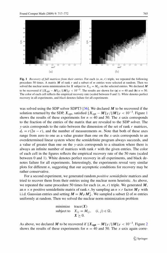
Found Comput Math (2009) 9: 717–772 765
Fig. 1 Recovery of full matrices from their entries. For each (n,m, r) triple, we repeated the followingprocedure 50 times. A matrix M of rank r and a subset of m entries were selected at random. Then wesolved the nuclear norm minimization for X subject to Xij = Mij on the selected entries. We declared M
to be recovered if ‖Xopt − M‖F /‖M‖F < 10−3. The results are shown for (a) n = 40 and (b) n = 50.The color of each cell reflects the empirical recovery rate (scaled between 0 and 1). White denotes perfectrecovery in all experiments, and black denotes failure for all experiments
was solved using the SDP solver SDPT3 [36]. We declared M to be recovered if thesolution returned by the SDP, Xopt, satisfied ‖Xopt − M‖F /‖M‖F < 10−3. Figure 1shows the results of these experiments for n = 40 and 50. The x-axis correspondsto the fraction of the entries of the matrix that are revealed to the SDP solver. They-axis corresponds to the ratio between the dimension of the set of rank r matrices,dr = r(2n − r), and the number of measurements m. Note that both of these axesrange from zero to one as a value greater than one on the x-axis corresponds to anoverdetermined linear system where the semidefinite program always succeeds, anda value of greater than one on the y-axis corresponds to a situation where there isalways an infinite number of matrices with rank r with the given entries. The colorof each cell in the figures reflects the empirical recovery rate of the 50 runs (scaledbetween 0 and 1). White denotes perfect recovery in all experiments, and black de-notes failure for all experiments. Interestingly, the experiments reveal very similarplots for different n, suggesting that our asymptotic conditions for recovery may berather conservative.
For a second experiment, we generated random positive semidefinite matrices andtried to recover them from their entries using the nuclear norm heuristic. As above,we repeated the same procedure 50 times for each (n,m, r) triple. We generated M ,an n×n positive semidefinite matrix of rank r , by sampling an n× r factor MF withi.i.d. Gaussian entries and setting M = MF M∗
F . We sampled a subset � of m entriesuniformly at random. Then we solved the nuclear norm minimization problem
minimize trace(X)
subject to Xij = Mij , (i, j) ∈ �,
X � 0.
As above, we declared M to be recovered if ‖Xopt − M‖F /‖M‖F < 10−3. Figure 2shows the results of these experiments for n = 40 and 50. The x-axis again corre-

766 Found Comput Math (2009) 9: 717–772
Fig. 2 Recovery of positive semidefinite matrices from their entries. For each (n,m, r) triple, we repeatedthe following procedure 50 times. A positive semidefinite matrix M of rank r and a set of m entrieswere selected at random. Then we solved the nuclear norm minimization subject to Xij = Mij on theselected entries with the constraint that X � 0. The color scheme for each cell denotes empirical recoveryprobability and is the same as in Fig. 1. The results are shown for (a) n = 40 and (b) n = 50
sponds to the fraction of the entries of the matrix that are revealed to the SDP solver,but in this case, the number of measurements is divided by Dn = n(n + 1)/2, thenumber of unique entries in a positive-semidefinite matrix and the dimension of therank r matrices is dr = nr − r(r − 1)/2. The color of each cell is chosen in the samefashion as in the experiment with full matrices. Interestingly, the recovery region ismuch larger for positive semidefinite matrices, and future work is needed to inves-tigate if the theoretical scaling is also more favorable in this scenario of low-rankmatrix completion.
Finally, in Fig. 3, we plot the performance of the nuclear norm heuristic whenrecovering low-rank matrices from Gaussian projections of these matrices. In thesecases, M was generated in the same fashion as above, but in place of sampling en-tries, we generated m random Gaussian projections of the data (see the discussion inSect. 1.4). Then we solved the optimization
minimize ‖X‖∗subject to A(X) = A(M),
with the additional constraint that X � 0 in the positive semidefinite case. Here, A(X)
denotes a linear map of the form (1.15) where the entries are sampled i.i.d. from azero-mean unit variance Gaussian distribution. In these experiments, the recoveryregime is far larger than in the case of that of sampling entries, but this is not par-ticularly surprising as each Gaussian observation measures a contribution from everyentry in the matrix M . These Gaussian models were studied extensively in [29].

Found Comput Math (2009) 9: 717–772 767
Fig. 3 Recovery of matrices from Gaussian observations. For each (n,m, r) triple, we repeated the fol-lowing procedure 10 times. In (a), a matrix of rank r was generated as in Fig. 1. In (b) a positive semidef-inite matrix of rank r was generated as in Fig. 2. In both plots, we select a matrix A from the Gaussianensemble with m rows and n2 (in (a)) or Dn = n(n + 1)/2 (in (b)) columns. Then we solve the nuclearnorm minimization subject to A(X) = A(M). The color scheme for each cell denotes empirical recoveryprobability and is the same as in Figs. 1 and 2
8 Discussion
8.1 Improvements
In this paper, we have shown that under suitable conditions, one can reconstruct ann × n matrix of rank r from a small number of its sampled entries provided that thisnumber is on the order of n1.2r logn, at least for moderate values of the rank. Onewould like to know whether better results hold in the sense that exact matrix recoverywould be guaranteed with a reduced number of measurements. In particular, recallthat an n × n matrix of rank r depends on (2n − r)r degrees of freedom; is it truethen that it is possible to recover most low-rank matrices from on the order of nr—up to logarithmic multiplicative factors—randomly selected entries? Can the samplesize be merely proportional to the true complexity of the low-rank object we wish torecover?
In this direction, we would like to emphasize that there is nothing in our ap-proach that apparently prevents us from getting stronger results. Indeed, we devel-oped a bound on the spectral norm of each of the first four terms (PT ⊥ P�PT )Hk(E)
in the series (4.13) (corresponding to values of k equal to 0,1,2,3) and used ageneral argument to bound the remainder of the series. Presumably, one couldbound higher order terms by the same techniques. Getting an appropriate bound on‖(PT ⊥ P�PT )H4(E)‖ would lower the exponent of n from 6/5 to 7/6. The appropri-ate bound on ‖(PT ⊥ P�PT )H5(E)‖ would further lower the exponent to 8/7, and soon. To obtain an optimal result, one would need to reach k of size about logn. In do-ing so, however, one would have to pay special attention to the size of the decouplingconstants (the constant CD for two variables in Lemma 6.5) which depend on k—thenumber of decoupled variables. These constants grow with k and upper bounds areknown [14, 15].

768 Found Comput Math (2009) 9: 717–772
8.2 Further Directions
It would be of interest to extend our results to the case where the unknown matrix isapproximately low-rank. Suppose we write the SVD of a matrix M as
M =∑
1≤k≤n
σkukv∗k,
where σ1 ≥ σ2 ≥ · · · ≥ σn ≥ 0 and assume for simplicity that none of the σk’s vanish.In general, it is impossible to complete such a matrix exactly from a partial subset ofits entries. However, one might hope to be able to recover a good approximation if, forexample, most of the singular values are small or negligible. For instance, considerthe truncated SVD of the matrix M ,
Mr =∑
1≤k≤r
σkukv∗k,
where the sum extends over the r largest singular values and let M� be the solutionto (1.5). Then one would not expect to have M� = M but it would be of great interestto determine whether the size of M� −M is comparable to that of M −Mr providedthat the number of sampled entries is sufficiently large. For example, one would liketo know whether it is reasonable to expect that ‖M� − M‖∗ is on the same order as‖M − Mr‖∗ (one could ask for a similar comparison with a different norm). If theanswer is positive, then this would say that approximately low-rank matrices can beaccurately recovered from a small set of sampled entries.
Another important direction is to determine whether the reconstruction is robustto noise as in some applications, one would presumably observe
Yij = Mij + zij , (i, j) ∈ �,
where z is a deterministic or stochastic perturbation. In this setup, one would perhapswant to minimize the nuclear norm subject to ‖P�(X − Y )‖F ≤ ε where ε is anupper bound on the noise level instead of enforcing the equality constraint P�(X) =P�(Y ). Can one expect that this algorithm or a variation thereof provides accurateanswers? That is, can one expect that the error between the recovered and the truedata matrix be proportional to the noise level?
This scenario was considered in [3] where it was shown that most of the entriescan be reconstructed to o(1) error by computing the singular value decompositionof the matrix which is equal to Mij when (i, j) ∈ � and zeros everywhere else. Thisbound translates into O(n) error in the Frobenius norm. An adaptation of the analysisto the nuclear norm minimization problem (1.5) rather than the SVD based algorithmcould lead to a better error estimate.
Finally, we note that the nuclear norm minimization problem (1.5) considered inthis paper is a highly structured semidefinite program. Standard interior point meth-ods will be impractical for problems where the unknown matrix has hundreds of rowsor columns. However, customized solvers designed to exploit the special structure ofthe nuclear norm and the sparsity of the constraints show a great deal of promise for

Found Comput Math (2009) 9: 717–772 769
solving incredibly large instances of the matrix completion problems. Since the dateof the original submission of this paper, preliminary research focusing on linearizedBregman schemes [8] have already demonstrated the solution of instances of the nu-clear norm minimization problem where the unknown matrix has tens of thousandsof columns; see also the fixed point continuation methods in [27]. Further investi-gation into such fast algorithms would make the theoretical guarantees developed inthis work practical for very large data analysis problems.
Acknowledgements E.C. was partially supported by a National Science Foundation grant CCF-515362,by the 2006 Waterman Award (NSF) and by an ONR grant. The authors would like to thank Ali Jadbabaie,Pablo Parrilo, Ali Rahimi, Terence Tao, and Joel Tropp for fruitful discussions about parts of this paper.E.C. would like to thank Arnaud Durand for his careful proofreading and comments.
Open Access This article is distributed under the terms of the Creative Commons Attribution Noncom-mercial License which permits any noncommercial use, distribution, and reproduction in any medium,provided the original author(s) and source are credited.
Appendix
A.1 Proof of Theorem 4.2
The proof of (4.10) follows that in [9] but we shall use slightly more precise estimates.Let Y1, . . . , Yn be a sequence of independent random variables taking values in a
Banach space and let Y� be the supremum defined as
Y� = supf ∈F
n∑i=1
f (Yi), (A.1)
where F is a countable family of real-valued functions such that if f ∈ F , then−f ∈ F . Talagrand [35] proved a concentration inequality about Y�; see also [23,Corollary 7.8].
Theorem A.1 Assume that |f | ≤ B and Ef (Yi) = 0 for every f in F and i =1, . . . , n. Then for all t ≥ 0,
P(|Y� − EY�| > t
)≤ 3 exp
(− t
KBlog
(1 + Bt
σ 2 + B EY�
)), (A.2)
where σ 2 = supf ∈F∑n
i=1 Ef 2(Yi), and K is a numerical constant.
We note that very precise values of the numerical constant K are known and aresmall; see [21].
We will apply this theorem to the random variable Z defined in the statement ofTheorem 4.2. Put Yab = p−1(δab − p) PT (eae
∗b) ⊗ PT (eae
∗b) and Y =∑
ab Yab . Bydefinition,

770 Found Comput Math (2009) 9: 717–772
Z = sup⟨X1, Y (X2)
⟩= sup∑ab
⟨X1, Yab(X2)
⟩
= sup p−1∑ab
(δab − p)⟨X1, PT (eae
∗b)⟩ ⟨
PT
(eae
∗b
),X2
⟩,
where the supremum is over a countable collection of matrices X1 and X2 obeying‖X1‖F ≤ 1 and ‖X2‖F ≤ 1. Note that it follows from (4.8)
∣∣⟨X1, Yab(X2)⟩∣∣= p−1 |δab − p| ∣∣⟨X1, PT
(eae
∗b
)⟩∣∣ ∣∣⟨PT
(eae
∗b
),X2
⟩∣∣
≤ p−1∥∥PT
(eae
∗b
)∥∥2F
≤ 2μ0r/(min(n1, n2)p
)= 2μ0 nr/m
(recall that n = max(n1, n2)). Hence, we can apply Theorem A.1 with B =2μ0(nr/m). Also,
E∣∣⟨X1, Yab(X2)
⟩∣∣2 = p−1(1 − p)∣∣⟨X1, PT
(eae
∗b
)⟩∣∣2 ∣∣⟨X2, PT
(eae
∗b
)⟩∣∣2
≤ p−1∥∥PT
(eae
∗b
)∥∥2F
∣∣⟨PT (X2), eae∗b
⟩∣∣2
so that∑ab
E∣∣⟨X1, Yab(X2)
⟩∣∣2 ≤ (2μ0 nr/m)∑ab
∣∣⟨PT (X2), eae∗b
⟩∣∣2
= (2μ0 nr/m)∥∥PT (X2)
∥∥2F
≤ 2μ0nr/m.
Since EZ ≤ 1, Theorem A.1 gives
P(|Z − EZ| > t
)≤ 3 exp
(− t
KBlog(1 + t/2)
)≤ 3 exp
(− t log 2
KBmin(1, t/2)
),
where we have used the fact that log(1 + u) ≥ (log 2) min(1, u) for u ≥ 0. Plugging
t = λ
√μ0 nr logn
mand B = 2μ0 nr/m establishes the claim.
A.2 Proof of Lemma 6.2
We shall make use of the following lemma which is an application of well-knowndeviation bounds about binomial variables.
Lemma A.2 Let {δi}1≤i≤n be a sequence of i.i.d. Bernoulli variables withP(δi = 1) = p and Y =∑n
i=1 δi . Then for each λ > 0,
P(Y > λ EY) ≤ exp
(− λ2
2 + 2λ/3EY
). (A.3)
The random variable∑
b δabE2ab is bounded by ‖E‖2∞
∑b δab and it thus suffices
to estimate the qth moment of Y∗ = maxYa where Ya =∑b δab . The inequality (A.3)
Found Comput Math (2009) 9: 717–772 771
implies that
P(Y∗ > λnp) ≤ n exp
(− λ2
2 + 2λ/3np
),
and for λ ≥ 2, this gives P(Y∗ > λnp) ≤ ne−λnp/2. Hence
EYq∗ =
∫ ∞
0P(Y∗ > t)qtq−1 dt ≤ (2np)q +
∫ ∞
2np
ne−t/2 qtq−1 dt.
By integrating by parts, one can check that when q ≤ np, we have
∫ ∞
2np
ne−t/2 qtq−1 dt ≤ nq (2np)q e−np.
Under the assumptions of the lemma, we have nq e−np ≤ 1 and, therefore,
EYq∗ ≤ 2 (2np)q.
The conclusion follows.
References
1. ACM SIGKDD, Netflix, Proceedings of KDD Cup and Workshop (2007). Proceedings available on-line at http://www.cs.uic.edu/~liub/KDD-cup-2007/proceedings.html.
2. T. Ando, R.A. Horn, C.R. Johnson, The singular values of a Hadamard product: A basic inequality,Linear Multilinear Algebra 21, 345–365 (1987).
3. Y. Azar, A. Fiat, A. Karlin, F. McSherry, J. Saia, Spectral analysis of data, in Proceedings of theThirty-third Annual ACM Symposium on Theory of Computing (2001).
4. C. Beck, R. D’Andrea, Computational study and comparisons of LFT reducibility methods, in Pro-ceedings of the American Control Conference (1998).
5. D.P. Bertsekas, A. Nedic, A.E. Ozdaglar, Convex Analysis and Optimization (Athena Scientific, Bel-mont, 2003).
6. B. Bollobás, Random Graphs, 2nd edn. (Cambridge University Press, Cambridge, 2001).7. A. Buchholz, Operator Khintchine inequality in non-commutative probability, Math. Ann. 319, 1–16
(2001).8. J.-F. Cai, E.J. Candès, Z. Shen, A singular value thresholding algorithm for matrix completion, Tech-
nical report (2008). Preprint available at http://arxiv.org/abs/0810.3286.9. E.J. Candès, J. Romberg, Sparsity and incoherence in compressive sampling, Inverse Probl. 23(3),
969–985 (2007).10. E.J. Candès, J. Romberg, T. Tao, Robust uncertainty principles: exact signal reconstruction from
highly incomplete frequency information, IEEE Trans. Inf. Theory 52(2), 489–509 (2006).11. E.J. Candès, T. Tao, Decoding by linear programming, IEEE Trans. Inf. Theory 51(12), 4203–4215
(2005).12. E.J. Candès, T. Tao, Near optimal signal recovery from random projections: Universal encoding strate-
gies?, IEEE Trans. Inf. Theory 52(12), 5406–5425 (2006).13. A.L. Chistov, D.Yu. Grigoriev, Complexity of quantifier elimination in the theory of algebraically
closed fields, in Proceedings of the 11th Symposium on Mathematical Foundations of Computer Sci-ence. Lecture Notes in Computer Science, vol. 176 (Springer, Berlin, 1984), pp. 17–31.
14. V.H. de la Peña, Decoupling and Khintchine’s inequalities for U -statistics, Ann. Probab. 20(4), 1877–1892 (1992).
15. V.H. de la Peña, S.J. Montgomery-Smith, Decoupling inequalities for the tail probabilities of multi-variate U -statistics, Ann. Probab. 23(2), 806–816 (1995).

772 Found Comput Math (2009) 9: 717–772
16. D.L. Donoho, Compressed sensing, IEEE Trans. Inf. Theory 52(4), 1289–1306 (2006).17. P. Drineas, M.W. Mahoney, S. Muthukrishnan, Subspace sampling and relative-error matrix approxi-
mation: Column-based methods, in Proceedings of the Tenth Annual RANDOM (2006).18. P. Drineas, M.W. Mahoney, S. Muthukrishnan, Subspace sampling and relative-error matrix approxi-
mation: Column-row-based methods, in Proceedings of the Fourteenth Annual ESA (2006).19. M. Fazel, Matrix rank minimization with applications, Ph.D. thesis, Stanford University (2002).20. R.A. Horn, C.R. Johnson, Topics in Matrix Analysis (Cambridge University Press, Cambridge, 1994).
Corrected reprint of the 1991 original.21. T. Klein, E. Rio, Concentration around the mean for maxima of empirical processes, Ann. Probab.
33(3), 1060–1077 (2005).22. B. Laurent, P. Massart, Adaptive estimation of a quadratic functional by model selection, Ann. Stat.
28(5), 1302–1338 (2000).23. M. Ledoux, The Concentration of Measure Phenomenon (AMS, Providence, 2001).24. A.S. Lewis, The mathematics of eigenvalue optimization, Math. Programm. 97(1–2), 155–176
(2003).25. N. Linial, E. London, Y. Rabinovich, The geometry of graphs and some of its algorithmic applications,
Combinatorica 15, 215–245 (1995).26. F. Lust-Picquard, Inégalités de Khintchine dans Cp (1 < p < ∞), C. R. Acad. Sci. Paris, Sér. I 303(7),
289–292 (1986).27. S. Ma, D. Goldfarb, L. Chen, Fixed point and Bregman iterative methods for matrix rank minimiza-
tion, Technical report (2008).28. M. Mesbahi, G.P. Papavassilopoulos, On the rank minimization problem over a positive semidefinite
linear matrix inequality, IEEE Trans. Automat. Control 42(2), 239–243 (1997).29. B. Recht, M. Fazel, P. Parrilo, Guaranteed minimum rank solutions of matrix equations via
nuclear norm minimization, SIAM Rev. (2007, submitted). Preprint available at http://arxiv.org/abs/0706.4138.
30. J.D.M. Rennie, N. Srebro, Fast maximum margin matrix factorization for collaborative prediction, inProceedings of the International Conference of Machine Learning (2005).
31. M. Rudelson, Random vectors in the isotropic position, J. Funct. Anal. 164(1), 60–72 (1999).32. M. Rudelson, R. Vershynin, Sampling from large matrices: an approach through geometric functional
analysis, J. ACM, 54(4), Art. 21, 19 pp. (electronic) (2007).33. A.M.-C. So, Y. Ye, Theory of semidefinite programming for sensor network localization, Math. Pro-
gram., Ser. B, 109, 2007.34. N. Srebro, Learning with matrix factorizations, Ph.D. thesis, Massachusetts Institute of Technology,
(2004).35. M. Talagrand, New concentration inequalities in product spaces, Invent. Math. 126(3), 505–563
(1996).36. K.C. Toh, M.J. Todd, R.H. Tütüncü, SDPT3—a MATLAB software package for semidefinite-
quadratic-linear programming. Available from http://www.math.nus.edu.sg/~mattohkc/sdpt3.html.37. L. Vandenberghe, S.P. Boyd, Semidefinite programming, SIAM Rev. 38(1), 49–95 (1996).38. G.A. Watson, Characterization of the subdifferential of some matrix norms, Linear Algebra Appl. 170,
33–45 (1992).

![Exact Matrix Completion via Convex Optimizationcandes/papers/MatrixCompletion.pdf · Exact Matrix Completion via Convex Optimization Emmanuel J. Cand esyand Benjamin Recht] yApplied](https://static.fdocuments.net/doc/165x107/5b3ffeab7f8b9a4b3f8cc56a/exact-matrix-completion-via-convex-optimization-candespapersmatrixcompletionpdf.jpg)