Ex-ante and ex-post evaluation of the 1989 French

welfare reform using a natural experiment : the 1908

social laws in Alsace-Moselle∗

July 18, 2011

Abstract

We use a combination of ex-ante and ex-post evaluation methods to evaluate

a major welfare policy implemented in France in 1989. The policy granted an

allowance (the Revenu Minimum d'Insertion, RMI, of up to 45% of the French

full time minimum wage) to every individual above age 25 and below a threshold

household income.

The ex-post evaluation relies on the speci�city of the Eastern part of France.

In Alsace-Moselle, since 1908 and during German occupancy, residents bene�ted

from a very similar transfer system (called �Aide Sociale�). Our estimates, based on

double and triple di�erences, show that the RMI policy was associated with: a 3%

fall in employment (among unskilled workers 25-55 years old), leading to an esti-

mated loss of 328 000 jobs; a decline in the job-access rate; and a 5-month increase

in the average duration of unemployment. We �nd considerably larger disincentive

e�ects for single parents. In a second step, we build and calibrate a matching model

with endogenous job search e�ort, using the di�erence-in-di�erences estimates. It

predicts that, if a 38% implicit tax rate had been maintained as in the 2007 reform

(RSA), instead of a 100% implicit tax rate due to the RMI, the increase in unem-

ployment would have been approximately half of its actual value, and the increase

in the duration of unemployment would have been limited to only 2.5 months.

Keywords: welfare policies, di�erence-in-di�erences, labor supply, job search.

JEL Classi�cation: J22.

∗The project was �nanced thanks to the grant EVALPOLPUB-2010 from ANR (French NationalResearch Agency). It was revised during a stay of the authors at the University of California, SantaBarbara, the hospitality of which is gratefully acknowledged. We thank the seminar participants atCarnegie-Mellon, Tepper School of Business and Univ. Lyon II, GATE, for helpful comments.

1

1 Introduction

Many European countries as well as some US states have experimented with givingdirect cash transfers to the poorest families and individuals in society. These welfarepolicies are thought to be a straightforward way of alleviating poverty and, to someextent, the side e�ects of poverty, such as crime, underinvestment in education, andhealth problems.

However, these bene�ts may come at a cost. Such policies may cause disincentivee�ects with respect to employment and labor market participation. Transferring cash topoor households may discourage job search e�orts and undermine work ethic. Answeringthese questions means understanding the negative income e�ect in labour supply curves,which several studies �nd evidence to support (see the comprehensive survey by Blundelland McCurdy 1999.)1.

In 1989, under the presidency of François Mitterrand, Michel Rocard's socialist gov-ernment passed the RMI law (Revenu Minimum d'Insertion), which provided incomesupport to all individuals above age 25 whose income fell below a certain threshold. Theamount was initially 2000 French Francs (about 300 euros) for a single person, roughly40% of the gross monthly minimum wage at the time (4,961.84 FF or about 800 euros),with additional bene�ts per dependent person in the household. Surprisingly, at the timeof the 1989 reform and in subsequent years, few attempts have been made to evaluatethe e�ects of the RMI on employment and unemployment. This may be explained bythe lack of appropriate data, the absence of a convincing identi�cation strategy, sometheoretical shortcomings, and perhaps politics' disinterest in scienti�c arguments2.

1During the 1980's, policies in many states and countries moved from welfare to workfare, wheretransfers are made conditional on working. Examples of workfare policies are either tax credits (such asthe earned income tax credit (EITC) in the US or the WTC in the UK) or wage subsidies adding up tothe net wage received by employers (such as the Self-Su�ciency project in Canada). The evaluation ofthese policies still amounts to knowledge of labor supply elasticities, but now the uncompensated laborsupply elasticities with respect to wages must be estimated.

2Many studies had to overcome the lack of information about eligibility of potential RMI recipientsand rely on proxies instead. The di�culty of obtaining a clear identi�cation strategy is due to the factthat France is a centralized country where laws are implemented all over the territory: the design ofappropriate control groups which could serve as counterfactuals, such as una�ected regions, is there-fore di�cult. The e�ects of major labor policies in France such as minimum wage changes, worktimereduction or payroll tax exemptions had to rely on creatively chosen control groups, for instance usingvariations in �rm size, such as Crépon and Kramarz (2002) or Crépon et al. (2004). With regard tothe lack of a fully-developed theory adapted to European labor markets, it is ackowledged that themeasurement of disincentive e�ects of welfare policies traditionally relies on compensated and uncom-pensated elasticities of labor supply with respect to earnings, e.g. see Blundell and McCurdy (1999).However, in Continental Europe, and in France in particular, the existence of high rates of involuntaryunemployment among the potential recipients implies that more complex models of labor supply areneeded. Those models should take into account the existence of several labor market states, and inparticular the existence of unemployment. Blundell and Mc Curdy (1999, pp 1686 to 1772) argued thatthe literature lacks a proper modelling of the process of job search and job matching.

2

In this paper, we attempt to overcome these many methodological di�culties intwo ways. First, we show that regional variance can in fact be found in France. Thisvariance comes not from the implementation of the RMI law, but instead from the pre-1989 situation. In particular, we make use of an interesting feature of French institutions:the Northeastern part of France (a region, Alsace, and a sub-region or �département�,Moselle) has had di�erent institutions from the rest of the country since the end of theXIX th century. In particular, Alsace-Moselle has had a di�erent social security system.This unique historical accident allows us to use a di�erence-in-di�erences framework toevaluate the reforms that were implemented di�erently in the rest of France. Alsace-Moselle can serve as a control group, while the rest of France can be used as the treatmentgroup3.

Applying this strategy, based on double and triple di�erence estimates to controlfor di�erent regional trends, we investigate the employment, unemployment and laborforce participation e�ects of RMI, as well as the e�ects on job search and wages. Weinclude a number of robustness checks and falsi�cation exercises. We then calibratekey parameters of an extension of the three-state labor market model, such that thedisincentive e�ects, according to the model and the di�erence-in-di�erences approach,are the same. Finally, we use the calibrated model to run a number of counterfactualpolicies, in particular the recent RSA reform. If that reform had been implementedcounterfactually in 1989, our model suggests that the employment losses would havebeen reduced by 50 percent.

Our paper is organized as follows: In Section 2, we outline the RMI experimentin France, the regional implementation in Alsace-Moselle and additional local socialpolicies, and brie�y survey earlier policy evaluations of it. In Section 3, we describethe data and the empirical methodology. In Section 4, we provide the main employmentand unemployment results and various additional robustness checks. In Section 5, wedevelop a job search model with social transfers and general equilibrium e�ects in orderto replicate the various possible channels through which the RMI may a�ect employmentand unemployment. We reach a number of predictions that �t the empirical �ndings.In Section 6, we then use the di�erence-in-di�erences results of Section 4 to calibrateour model, and we run a number of counterfactual experiments. Section 7 concludes.

3This identi�cation strategy was successfully applied to the evaluation of another policy, the e�ectsof the 35h workweek reform in 1998 in Chemin and Wasmer (2009).

3

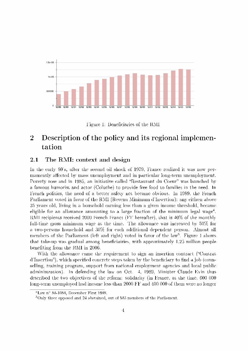
Figure 1: Bene�ciaries of the RMI

2 Description of the policy and its regional implemen-

tation

2.1 The RMI: context and design

In the early 80's, after the second oil shock of 1979, France realized it was now per-mamently a�ected by mass unemployment and in particular long-term unemployment.Poverty rose and in 1985, an initiative called �Restaurant du Coeur� was launched bya famous humorist and actor (Coluche) to provide free food to families in the need. InFrench politics, the need of a better safety net became obvious. In 1989, the FrenchParliament voted in favor of the RMI (Revenu Minimum d'Insertion): any citizen above25 years old, living in a household earning less than a given income threshold, becameeligible for an allowance amounting to a large fraction of the minimum legal wage4.RMI recipients received 2000 French Francs (FF hereafter), that is 40% of the monthlyfull-time gross minimum wage at the time. The allowance was increased by 50% fora two-persons household and 30% for each additional dependent person. Almost allmembers of the Parliament (left and right) voted in favor of the law5. Figure 1 showsthat take-up was gradual among bene�ciairies, with approximately 1.25 million peoplebene�ting from the RMI in 2006.

With the allowance came the requirement to sign an insertion contract (�Contratd'Insertion�), which speci�ed concrete steps taken by the bene�ciary to �nd a job (coun-selling, training program, support from national employment agencies and local publicadministration). In defending the law on Oct. 4, 1989, Minister Claude Evin thusdescribed the two objectives of the reform: solidarity (in France, at the time, 600 000long-term unemployed had income less than 2000 FF and 400 000 of them were no longer

4Law n◦ 88-1088, December First 1988.5Only three opposed and 24 abstained, out of 585 members of the Parliament.

4

covered by social security); and individual responsibility (the �Contrat d'Insertion� aimedat reinserting individuals into the labor market). The RMI policy was initially presentedas a mix of welfare and workfare: the transfer would be made conditional on an objectiveof 'insertion' into employment and society, thanks to counselling, provision of incentivesand housing allowance.

However, the insertion contract was not always enforced. In fact, only 60 percent ofrecipients signed (Zoyem, 2001). The President of the Parliament Commission in chargeof the examination of the law, MP Jean-Michel Belorgey, even argued that it would beunthinkable to cut bene�ts to those unable to get a job, given that failure to �nd workmay be due to �de�ciencies of the public administration� in re-inserting recipients intothe labor market.

Several academic works, including Gurgand and Margolis (2001, 2005), pointed outthat the gains from activity may be small for many RMI recipients. This phenomenonis known as a poverty trap: that is, an implicit marginal tax rate of 100%, or evenhigher, for RMI recipients who obtain a job. In addition, jobs taken by RMI recipientswere generally low-paying, on average 610 euros per month according to Rioux (2001).Piketty (1998) highlighted women's high labor supply elasticities and the disincentivee�ects of policies such as RMI and family transfers. In an e�ort to mitigate this, partialreforms were implemented in 1998, 2000 and 2001 (Hagnéré and Trannoy, 2001) toraise the incentives to work. Despite the warnings, the RMI rapidly became the largestwelfare program in France: in December 2007, the RMI was distributed to 1.16 millionrecipients, roughly the total number of unemployed workers.

Policy debates gradually came to the consensus that the �insertion component� ofRMI had not succeeded, even though few explicitly recognized the disincentive e�ects.In theory, such e�ects should exist: the RMI was indeed a �di�erential allowance�. Aftera transition period, all income from activity led to an equivalent decrease in the amountof the allowance, leading to a 100% e�ective marginal tax rate. In some cases, themarginal hours worked would reduce the income of RMI recipients, given the cumulatedloss of RMI and other social transfers. To limit the disincentive e�ects of this 100%implicit marginal tax rate of labor income, which in some cases would be even largerdue to the loss of additional social transfers (free public transportation in some regionssuch as Ile de France, rebates of 10 euros on monthly telephone bills in France Telecom,and so on), the initial transition period during which RMI and labor incomes could becumulated was then extended from 3 months to 12 months in the 2000's. According toHagneré et Trannoy (2001), after 1998, the �rst three months of labor income would notbe counted into the determination of the level of RMI, and the next 9 months would becounted with a rebate of 50%, leading to a smaller e�ective marginal tax rate during thistransition period. Nevertheless, after the one year period, the marginal rate of taxationwould increase again to 100%.

In 2007, another major reform led by Martin Hirsch (Haut Commissaire aux Solidar-ités Actives) took stock of this debate and introduced better incentives: for the marginal

5

hours worked, the new scheme (RSA, standing for Revenu de Solidarité Active) trans-formed each additional euro of labor income into 0.62 euro of additional net income,equivalent to a much lower 38% e�ective marginal tax rate. The RSA combined theRMI (RSA socle) and a complement, proportional to the additional labor income (RSAchapeau).

2.2 Alsace-Moselle : �aide sociale�

A system (�aide sociale�) similar to the RMI, at the city level, was already in placein Alsace Moselle. Since 1908, all municipalities in Alsace-Moselle were required toprovide assistance to impoverished citizens6. For instance, in the main city in Alsace(Strasbourg), the allowance for a single eligible person amounts to 65% of the grossminimum wage (Kintz, 1989). It was also more generous than the RMI in that itconcerned all individuals above 16 years old 7.

After the introduction of the French RMI in 1989, municipalities in Alsace-Mosellemay still provide an allowance to poor individuals, but this allowance reduces the RMIgiven by the state (Woehrling, 2002)8. Consequently, after 1989, cities in Alsace Mosellehave a direct incentive to stop providing this �aide sociale�, as emphasized by Woehrling(2002). Poor individuals qualify for welfare payments in Alsace Moselle and the rest ofFrance after 1989, but only in Alsace Moselle before 1989. This provides an opportunityfor a di�erence-in-di�erence analysis before and after 1988, between Alsace Moselle andthe rest of France, in order to evaluate the impact of the RMI.

Of course, one may argue that Alsace-Moselle is di�erent due to the existence ofother regional speci�cities. In Figure 2, Alsace-Moselle is represented by the three�départements� labeled 57, 68 and 67. They are in the top east corner of France, andhappen to be the only to be ones with a border with Germany.

This has at least one undesirable consequence for the econometric identi�cation:since the pattern of trade between Germany and France is not homogeneous on French

6�Lois locales des 30 mai 1908 et du 8 novembre 1909�.http://www.lexisnexis.com/fr/droit/search/runRemoteLink.do?bct=A&risb=21_T4090933869&homeCsi=303228&A=0.7883780303835484&urlEnc=ISO-8859-1&&dpsi=0ARX&remotekey1=DOC-ID&remotekey2=685_EN_AL0_64685FASCICULEEN_1_PRO_018548&service=DOC-ID&origdpsi=0ARX&level=1&duRemote=true. French central state never abolished

the various local social laws including this speci�c one, and even recognized o�cially the Alsace-Mosellespeci�city in a law text in 1924. See Chemin and Wasmer (2009).

7According to Kintz (1989), in Strasbourg there are 13 000 persons coveredby the subsidies for anamount of near 3 millions euros. In some other cities, e.g. Colmar, in-kind allowances are distributed tothose in need. A decree-law from 1938 excluded foreigners. This disposition, according to Kintz (1989)is not really applied and in any event cannot legally be applied to European Union citizens. Kintz alsoargue that the system is much less known in the �département� of Moselle.

8The amount of RMI given is equal to a minimum revenue of approximately 450 euros minus income.

6

Figure 2: Map of France

territory, but instead depends on distance to the border as any gravity model pre-dicts, it is quite likely that Alsace-Moselle is disproportionately a�ected by the Ger-man economic cycle when it di�ers from the French economic cycle. In such a case,any comparison of �before and after� in Alsace-Moselle and the rest of France will becontaminated by spillover e�ects. To solve this di�cult issue, we will need to do sev-eral additional comparisons with una�ected groups in both Alsace-Moselle and the restof France. These amount to falsi�cation exercises or triple di�erences, combining thedi�erence-in-di�erences results of the a�ected and una�ected.

2.3 Other local transfers

In the early discussion of the law, Claude Evin noted that some places in France hadalready implemented a type of social help. He gave the example of two départements (Ile-et-Vilaine, dept #35, in Britanny, and Territoire de Belfort, dept #90, next to Alsace)and cities (Besançon, in Doubs, dept #25, next to Territoire de Belfort ; Grenoble, inIsère, dept #38, in French Alps). Interestingly enough, neither he nor the Rapporteurof the project, Belorgey, mentioned Alsace and Moselle social laws, despite the evidentimportance of local social laws in the region. Kintz (1989) recalls that �local social aid isone of the less known sector of local laws in Alsace-Moselle and points out some errorsor omissions about the local system in the early discussions at the French Parliament�.

7

2.4 A survey of the literature

A comprehensive survey of the RMI and the debate regarding its evolution during its�rst decade can be found in L'Horty and Parent (1999). In addition to the papersalready cited in Section 2.1, the existing literature points to the strong disincentivee�ects of the RMI. Rioux (2001) �nds that RMI recipients search for a job less than theunemployed not receiving bene�ts. Using case studies, Gurgand and Margolis (2001)�nd that gains from �nding a job are low for RMI recipients. In particular, more thanhalf of single mothers would see their income decrease if they were to take a job. Zoyem(2001) showed that 40% of RMI recipients never signed a �contrat d'insertion socialeou professionnelle�, the contract specifying the path towards insertion. He also showedthat the transition through those contracts for the other 60% only had marginal e�ectson job placement: he only found a signi�cant e�ect on placement in subsidized jobs(local public services or local administrations) and insigni�cant e�ects on placementinto temporary or permanent private sector jobs.

Terracol (2009), using data on the French part of the European Community House-hold Panel, managed to calculate the eligibility of recipients and found adverse e�ects ofeligibility on �nding a job in a duration model. Bargain and Doorley (2009), using a re-gression discontinuity approach based on age � childless adults below 25 are not eligible �also found strong e�ects on employment, a -7 to -10% employment e�ect for uneducatedmen. Overall, the literature shows disincentive e�ects, despite partial reforms to reducepoverty traps (Hagnéré and Trannoy, 2001)9.

3 Empirical methodology

Given the literature described above and simple theoretical reasoning, one may be willingto test whether the RMI has the following e�ects:

1. A decline in the search e�ort of job seekers, all the more when available jobs arepart-time.

2. A decrease in employment due to a wage-push e�ect of the policy.3. A rise in unemployment due to lower e�ort and lower job creation.4. An increase in the number of unemployed coming from inactivity due to �labeling

e�ects�. That is, non-searching workers claiming RMI bene�ts and falsely counted asunemployed.

To investigate these e�ects, we compare the more than 25 years old to the less than25 years old (not a�ected by the RMI), in the rest of France compared to Alsace-Moselle,

9In 1998 and 2001, the transitory period during which a cumul of labor earnings and social minimawas allowed (initially 3 months) was extended. After 2000, the amount of the housing allowance wascalculated without taking into account a part of the labor earnings below the RMI. Finally, the �Primepour l'Emploi� (a moderate wage subsidy enacted through the tax system, with a negative income taxcomponent) was introduced in 2001.

8

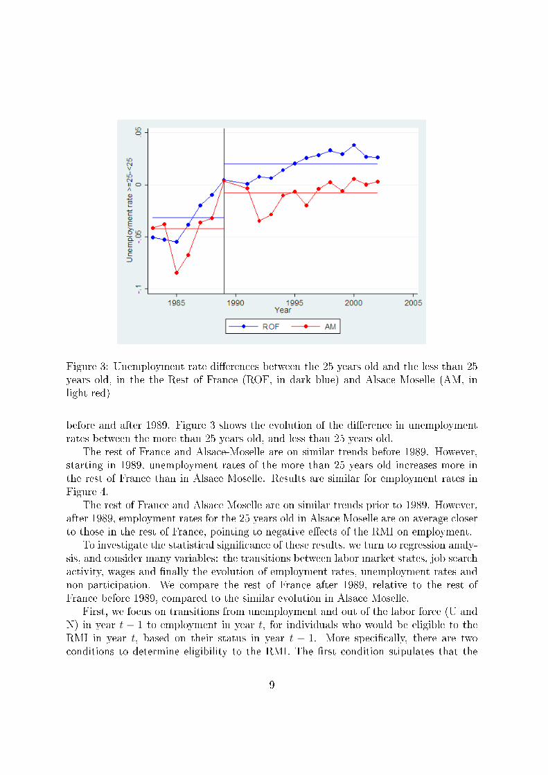
Figure 3: Unemployment rate di�erences between the 25 years old and the less than 25years old, in the the Rest of France (ROF, in dark blue) and Alsace Moselle (AM, inlight red)

before and after 1989. Figure 3 shows the evolution of the di�erence in unemploymentrates between the more than 25 years old, and less than 25 years old.

The rest of France and Alsace-Moselle are on similar trends before 1989. However,starting in 1989, unemployment rates of the more than 25 years old increases more inthe rest of France than in Alsace Moselle. Results are similar for employment rates inFigure 4.

The rest of France and Alsace Moselle are on similar trends prior to 1989. However,after 1989, employment rates for the 25 years old in Alsace Moselle are on average closerto those in the rest of France, pointing to negative e�ects of the RMI on employment.

To investigate the statistical signi�cance of these results, we turn to regression analy-sis, and consider many variables: the transitions between labor market states, job searchactivity, wages and �nally the evolution of employment rates, unemployment rates andnon-participation. We compare the rest of France after 1989, relative to the rest ofFrance before 1989, compared to the similar evolution in Alsace Moselle.

First, we focus on transitions from unemployment and out of the labor force (U andN) in year t − 1 to employment in year t, for individuals who would be eligible to theRMI in year t, based on their status in year t − 1. More speci�cally, there are twoconditions to determine eligibility to the RMI. The �rst condition stipulates that the

9

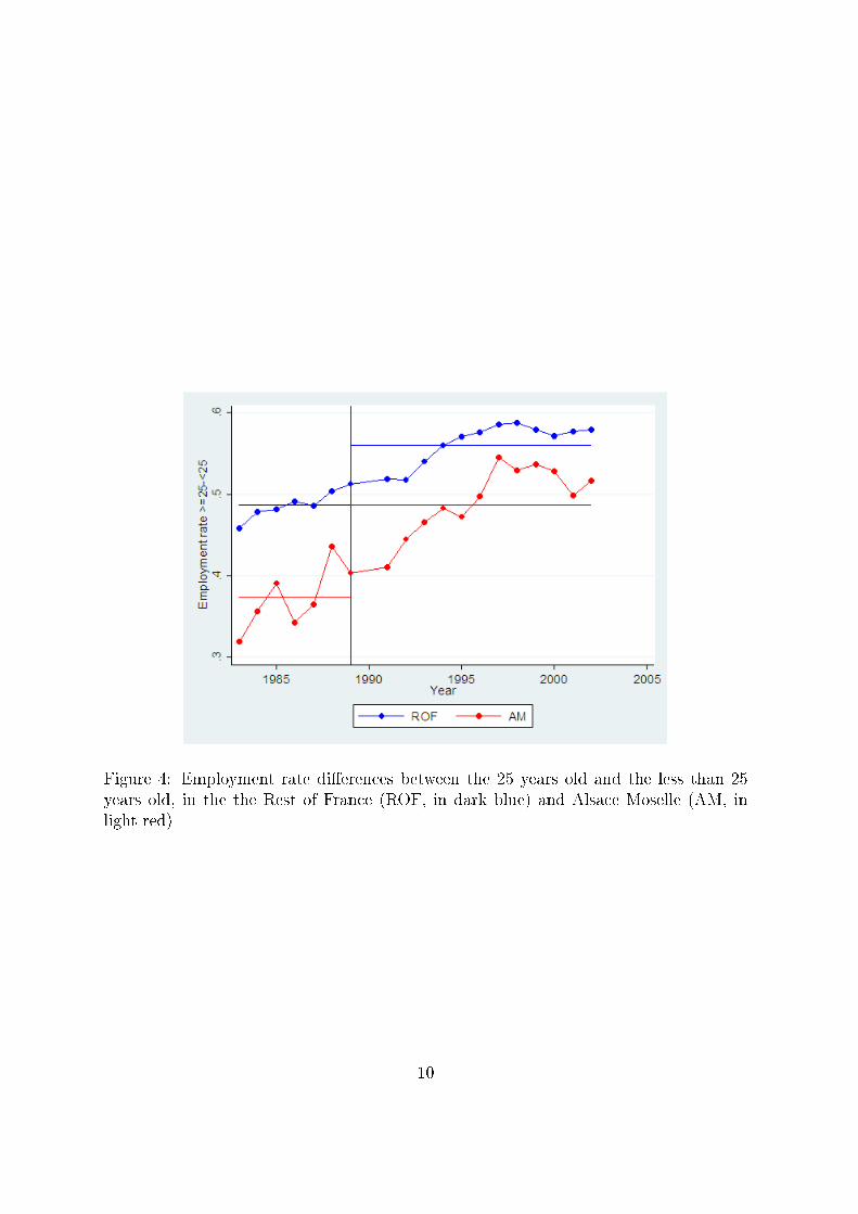
Figure 4: Employment rate di�erences between the 25 years old and the less than 25years old, in the the Rest of France (ROF, in dark blue) and Alsace Moselle (AM, inlight red)

10

individual must be more than 25 years old. The second condition states that quarterlytotal household income10 must be inferior to a certain level11.

To obtain information on a certain individual the year before, we use the longitudinalnature of France's Labor Force Survey, the Enquête Emploi. This survey is collectedevery year in March. The random and representative sample is partly renewed everyyear: only a third of the households in the sample are surveyed again the next year,and overall each household is interviewed three times. In this paper, we keep all theindividuals for which we have information the year before. This represents 1,539,167such individuals between 1982 and 2002 (see Appendix Table 1 for descriptive statisticsof this sample). Given our identi�cation strategy, which is based on three �départements�representing a relatively small fraction of France, the Labor Force Survey represents thebest possible data, because its size allows for a large enough control group.

We then focus on eligible, i.e. low income, households. In France, the duration ofunemployment bene�ts was calculated on the basis of tenure in the previous job. Inparticular, in 1989, individuals are granted a proportion of their past income during 3,15, or 30 months, if they have worked respectively 4, 8, or more than 12 months in theirpast job (Daniel, 1999). One can thus safely assume that an individual more than 24years old, AND in a low-income household, AND who has been unemployed for morethan 20 months the year before or is out of the labor force, is eligible for the RMIa year after, i.e. 12 months later, if he remains unemployed, as his unemploymentinsurance runs out.

The drawback of this strategy is that we only observe income in the previous year,and not in the previous quarter. Hence, the eligibility is subject to measurement error.An implication of this is that the e�ects we will estimate in the regression analysis arelikely to be underestimating the true coe�cients. We will therefore need to interpretour results as a possible lower bound of our estimates12.

In this sample, we �nd 44,663 individuals of more than 24 years old, AND in a low-income household, AND who have been unemployed for more than 20 months or out ofthe labor force the year before. Note that these individuals are eligible to the RMI

10Total income includes income from all possible sources (wage, bonus, in-kind payments, unem-ployment insurance, "allocations familiales", "allocations logement", pro�t from �rms or agriculturalexploitation, pensions, real estate revenues, alimonies, unemployment insurance).

11The maximum RMI amount in 1989 is 2000FF/month for a single individual. It is re-evaluated bydecree every year. We collected these decrees for every year after 1989. However, there was no RMIbefore 1989. To determine the maximum RMI amount that could have been obtained before 1988 (andthus a theoretical eligibility had the RMI been instituted), we de�ate the 1988 maximum RMI amountby the Consumer Price Index. Indeed, L'Horty et al (1999) discuss the indexation of the RMI based onthe consumer price index in France.

12In this sense, we follow the earlier papers such as Piketty (1998) who used the Labor Force Survey.We have less precise data than in Terracol (2009) who uses the French data of the European CommunityPanel with detailed information of monthly income. However, this panel only starts in 1994 and is notappropriate for our identi�cation strategy, beyond the too limited sample size in Alsace-Moselle.

11

in year t only if t ≥ 1989 in the rest of France, as the RMI was enacted in 1989. Incontrast, such individuals are eligible to the RMI for all years t in Alsace-Moselle, as theRMI is available in Alsace Moselle before (under the form of the �aide sociale�) and after1989. In this paper, we compare the transitions back to employment of these eligibleindividuals before and after 1989, in the rest of France compared to Alsace-Moselle.

The disincentive e�ects of the RMI, if they exist, imply that individuals are less likelyto get a job if they can bene�t from the RMI. Thus, we should see fewer transitions backto employment for eligible individuals in the rest of France after 1989, relative to the restof France before 1989. We should observe no di�erences in Alsace Moselle in the extentof these transitions before and after 1989, as the RMI is available to eligible individualsbefore and after. Thus, Alsace Moselle is an ideal control group for the rest of France.This forms the basis of a di�erence-in-di�erences analysis. Formally, we will performregressions of the following form:

∆employmentijt = αj + βt + γ1(Rest_of_France) ∗ (After1989)ijt + θXijt + uit (1)

where i corresponds to individual i, j to department j and t to year t. The dependentvariable ∆employmentijt is a dichotomous variable equal to 1 if the individual is workingat time t, 0 otherwise. It may be interpreted as a transition from unemployment orinactivity (U and N) to employment, as we focus on individuals unemployed or out ofthe labor force at time t− 1. αj are department �xed e�ects (95), and βt are year �xede�ects (20). (Rest_of_France) ∗ (After1989)ijt is an interaction term between thetwo following dichotomous variables. Rest_of_Francej is a dichotomous variable thattakes the value 1 if individual i resides in the rest of France, 0 otherwise. After1989tis a dichotomous variable that takes the value 1 if individual i is interviewed after1989, 0 otherwise. The coe�cient of interest is γ1, which measures the relative increasein transitions to employment for individuals in the rest of France after the reform.Additionally, 22 control variables (5 age dummies, sex, household size and 15 diplomadummies) are included in the analysis. Standard errors are clustered at the level ofthe department to account for serial correlation within department, the unit at whichthe reform is implemented (Moulton, 1990), that may arise in a di�erence-in-di�erencesestimation (Bertrand et al, 2004).

4 Results

4.1 Preliminary investigation: double-di�erence results

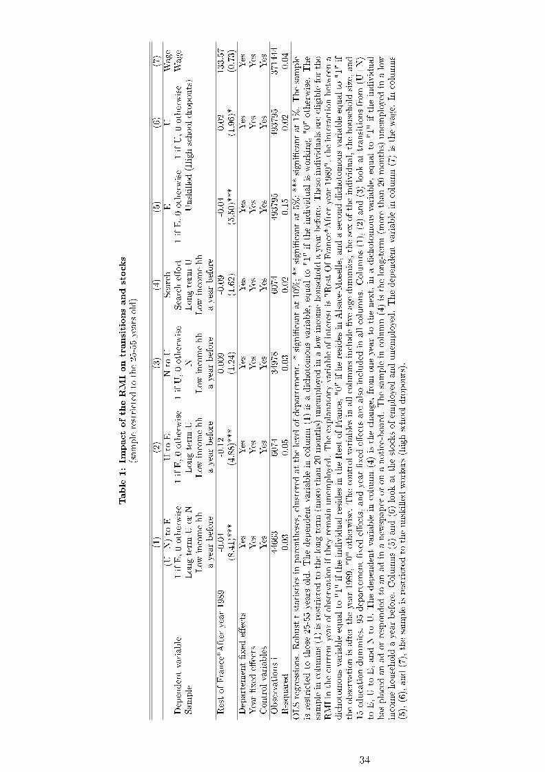
Table 1 looks at the impact of the RMI on transitions, search e�ort, stocks, and wages,based on double di�erence. The next sub-section provides additional causal evidencebased on triple di�erences. In column (1), the sample is restricted to individuals more

12

than 24 years old, AND in a low-income household, AND who have been unemployedfor more than 20 months, or out of the labor force, in year t− 1; in other words eligibleto the RMI in year t. The coe�cient γ1 of the variable �Rest of France*After year 1989�re�ects the e�ect of the RMI on the hazard rate into employment. This coe�cient islarge and negative: it is equal to -0.04, meaning that the probability of �nding a jobis 4 percentage points lower for an eligible individual in the rest of France after 1989,relative to a similar eligible individual in the rest of France before 1989, compared tothe same evolution for eligible individuals in Alsace-Moselle before and after 1989. Thisresult is statistically signi�cant at the 1 percent level. This is suggestive of disincentivee�ects: individuals with access to the RMI are less likely to get back to work. This 4percentage point decrease is a sizeable e�ect, considering that only 10 percent of suchindividuals get a job.

In column (2), the coe�cient is also large and signi�cantly negative on transitionsfrom U to E. This could be due in part to a composition e�ect of the pool of theunemployed itself, which we term the �labeling e�ect�: individuals not searching, thatis, theoretically out of the labor force, may have had an incentive to falsely declarethemselves unemployed, either because they felt this would help obtain the RMI orbecause of a feeling of guilt with respect to the interviewers.

To investigate, at least in part, the existence of this phenomenon, we may look attransitions from N to U. In column (3), the sample is restricted to out of the labor forceindividuals, more than 24 years old, in a low-income household in year t − 1; in otherwords eligible to the RMI in year t. The dependent variable is a dichotomous variable,equal to �1� if the individual is unemployed, �0� otherwise. The coe�cient is positive butnot signi�cant, which points to a weak �labeling e�ect�. This change in the compositionof the pool of the unemployed due to false declaration about job search activity andfalse labeling of Labor Force Statistics may therefore not be the main reason behind thelower hazard rate.

Column (4) looks at search e�ort of the unemployed workers. The dependent variablein column (4) is the change, from one year to the next, in a dichotomous variable, equalto �1� if the individual has placed an ad, or responded to an ad in a newspaper or ona notice-board13. The sample in column (4) is the long-term (more than 20 months)unemployed in a low income household a year before. Search e�ort decreases, but notsigni�cantly so.

13There are generally two ways to search for a job. First, an individual may place an ad, or respondto an ad, in a newspaper or on a notice-board of the governmental organizations (ANPE). This optionis chosen by 32 percent of the individuals looking for a job in France. Second, an individual may pursuea more proactive approach, by registering in a temporary work agency, contacting directly employers,or looking for a job through personal relationships. 99 percent of the individuals follow (or at leastself-report that they follow) this option. Considering the low variability in the second option, we preferto focus on the �rst option, i.e. placing or responding to an ad in a newspaper or on a notice-board.We �nd no e�ect of the RMI on the more proactive ways to search for a job.

13

Columns (5) and (6) look at the stocks of employed and unemployed. The sampleis restricted to the unskilled workers (high school dropouts). In column (5), the depen-dent variable is a dichotomous variable, equal to �1� if the individual is employed, �0�otherwise. The probability of being employed decreases by 4 percentage points. Thisindicates strong disincentive e�ects on unskilled workers. Column (6) indicates thatunemployment rises. Column (7) looks at wages, and �nds no signi�cant impact onwages.

Table 1 has presented evidence that the RMI is associated with quite strong disincen-tive e�ects. The results are based on simple di�erence-in-di�erences analysis between therest of France and Alsace-Moselle, before and after 1989. The main assumption on whichthis analysis relies is the �common time e�ects� assumption: to interpret causally thedi�erence-in-di�erences coe�cient, one needs to assume that the treatment and controlgroup are on the same time trend. In other words, the rest of France would have evolvedthe same way Alsace-Moselle did had the RMI not been implemented. This is certainlya strong assumption considering some inherent characteristics of Alsace Moselle, for ex-ample, its close proximity to Germany, which may have experienced an economic upturnover the same period.

4.2 Benchmark estimates: triple di�erences

We address this concern by performing triple di�erences. We use the individuals lessthan 25 years old, as a category knowingly not a�ected by the RMI. The RMI onlyapplies to individuals above 25 years14, whereas �aide sociale� in Alsace Moselle appliesto individuals of more than 16 years old. This means that individuals less than 24 yearsold a year before are not a�ected by the RMI in France, and are a�ected by the �aidesociale� in Alsace Moselle, before and after 1989. Using the less than 25 years old ina triple di�erences analysis is a strong test of the �common time e�ects� assumption.The �common time e�ects� assumption is replaced by a new, less demanding, one: thatindividuals below or above 25 years old are subject to the same relative trend in Alsace-Moselle with respect to the rest of France.

The sample in Table 2 includes individuals aged above and below 25 years old.We de�ne �More than 25� as a dichotomous variable equal to �1� if the individualsis more than 25 years old, �0� otherwise. We then interact this dichotomous variablewith all variables contained in the di�erence-in-di�erences analysis of equation (2), i.e.(Rest_of_France) ∗ (After1989)ijt, the department and year �xed e�ects. The coe�-cient of interest is now in front of (Rest_of_France)∗(After1989)∗(More_than_25)ijt,a triple di�erences coe�cient.

Column (1) shows that the probability to �nd a job is 7 percentage points lower

14It also applies to individuals below 25 but with dependent children and an income level below thethreshold. This very rarely happens in the data.

14

after the RMI was implemented in France. This is in contrast to the individuals lessthan 25 years old, who did not experience such a decrease. Columns (2) to (7) replicatethe analysis performed in Table 1, but in a triple di�erences framework. Consistentwith Table 1, Table 2 shows a negative impact on transitions from U to E (column (2)),no impact on transitions from N to U (the �labeling e�ect� in column (3)), a decreasein search e�ort (column (4)). The probability to be employed decreases (column (5)),while the probability to be unemployed increases (column (6)). No such e�ect is foundon wages as indicated in column (7).

These e�ects are large in magnitude. For example, column (1) indicates a sevenpercentage point decrease in the probability of transitioning to employment from un-employment or from being out of the labor force. Appendix Table 1 shows that suchindividuals represent 5 percent of the unskilled population between 25 and 55 years old,or approximately 15 million people.15 The RMI thus caused 52,50016 people to remainunemployed or out of the labor force because of disincentive e�ects. Column (6) showsa 3 percentage point reduction in total employment. Considering that 73 percent of thetotal population is employed, this represents 328, 500 individuals17.

4.3 Heterogeneous e�ects

Table 3 looks at the impact of the RMI more speci�cally on part-time workers and ondi�erent household compositions.

Column (1) shows the full sample result (as in of column (1) of Table 2). Column(2) instead restricts the analysis to part-time workers. The dependent variable is adichotomous variable, equal to �1� if the individual is employed part-time, �0� otherwise.The RMI has an e�ect on part-time work but not full-time work, as seen in column (3).This is expected since the disincentive e�ects are stronger for part-time work than forfull-time work.

Column (4) to (7) restrict the sample to di�erent household compositions (singlepersons, single parents, couples without children, couples with children). Column (5)indicates that the e�ect of the RMI is mostly felt by single parents, a fact consistentwith the existing literature (e.g. Piketty 1998, Gurgand and Margolis 2001).

4.4 Other checks: robustness and falsi�cation

The methodology is simple and transparent and can therefore be extended along severaldimensions. For the sake of concision, we will place several additional tables in the

15Source: http://www.insee.fr/fr/themes/tableau.asp?reg_id=0&ref_id=NATnon02150 Répartitionde la population par sexe et âge au 1er janvier 2011. Insee, estimations de population (résultatsprovisoires arrêtés �n 2010).

167%*5%*15 millions.173%*73*15 millions.

15

Appendix (Appendix Tables 2 to 4) and only brie�y describe the results. First, wevary the duration of the unemployment spell to show that the results are not sensitiveto the particular measure of eligibility used, or the focus on individuals having beenunemployed for more than 18 and 22 months the year before. The results remain verysimilar (see results in Appendix Table 2). We also removed the 22 control variables(5 age dummies, sex, household size and 15 diploma dummies), with no change in theresults: the results are not particularly sensitive to the particular set of control variablesused.

A concern with this estimation is the long time frame used. We use the EnquêteEmploi from 1982 to 2002. This long time span is advantageous because it gives alarge sample size, but the drawback is the possibility that many other things could havehappened in the rest of France compared to Alsace Moselle over this period. We thusrestricted the sample from 1985 to 1995. Results are robust to this restricted sample.

We then perform a falsi�cation exercise by looking at a period slightly before theenactment of the RMI, in column (6) of Appendix Table 2. For instance, we focus on theperiod 1984-1985, and look at the interaction term (Rest_of_France)∗(After1985)ijt.There was no RMI in France before or after 1985, while there was the �aide sociale� inAlsace-Moselle over the same period. Thus, we should see no signi�cant di�erence-in-di�erences coe�cient, as there has been no change in the rest of France over the period.Indeed, the di�erence-in-di�erences coe�cient of this regression are not signi�cantlydi�erent from zero. This indicates that the individuals considered, i.e. more than 24years old, AND in a low-income household, AND with no household members earningunemployment insurance, AND who have been unemployed for more than 20 months,or are out of the labor force, in year t− 1, evolve in a same manner in the rest of Franceor in Alsace-Moselle, in a period preceeding the enactment of the RMI.

We also remove in column (7) the départements of Ile-et-Vilaine (35), Doubs (25),Territoire de Belfort (90), and Isere (38) from the sample as some sort of �aide sociale�already existed in some of their municipalities, as explained in Section 2.3; and resultsdo not change.

We �nally present another triple di�erences analysis. Focusing on individuals thatare more than 24 years old, AND unemployed for more than 20 months or out of thelabor force, in year t−1, but who live in a household whose members earn more than themaximum RMI amount, we obtain a group of individuals similar in many dimensionsto the eligible individuals, but they are ineligible to the RMI in year t. In column(8) of Appendix Table 2, we �nd no impact on the transitions back to employmentof these individuals, before and after 1989, in the rest of France compared to Alsace-Moselle. Column (9) performs a triple di�erence analysis using these two categories ofindividuals. We de�ne �Long term-low income a year before�, as a dichotomous variableequal to �1� if the individuals is more than 24 years old, AND in a low-income household,AND with no household members earning unemployment insurance, AND who has beenunemployed for more than 20 months or out of the labor force, in year t− 1, �0� if the

16

individual is more than 24 years old, AND in a high-income household, AND who hasbeen unemployed for more than 20 months, or out of the labor force, in year t − 1.We interact this dichotomous variable with all variables contained in the di�erence-in-di�erences analysis, i.e. (Rest_of_France) ∗ (After1989)ijt, the department and year�xed e�ects. Column (9) shows that eligible individuals experience a 3 percentage pointdecline in their probability ofreturning to work due to the RMI.

4.5 Regression discontinuity design

Following Lemieux et al. (2008) in response to Fortin et al. (2004), we also perform aregression discontinuity design to estimate the impact of the RMI on employment. After1989, in the rest of France, only individuals more than 25 years old were eligible to theminimum income. We use this sharp discontinuity to compare the employment probabil-ities of individuals just above 25 years old compared to thosejust below 25 years old. Asopposed to the di�erence-in-di�erences estimator, we do not need to make assumptionsabout the comparability of the treated group to a control group that is temporally orgeographically distinct (Lemieux et al., 2008). A regression discontinuity design controlsfor the changing macroeconomic environment. Conditional on the assumption that in-dividuals do not manipulate their age to bene�t from the minimum income, being moreor less than 25 years old at the time of the survey is essentially random (Lee, 2008).Following Lemieux et al. (2008), we focus our analysis on high school dropouts18. Weperform regressions of the following form:

employmentijt = αj + βt + γ1(More_than_25)ijt + δ(age) + θXijt + uit (2)

where the dependent variable employmentijt is a dichotomous variable equal to 1 if theindividual is working at time t, 0 otherwise. The variable of interest is �More than 25�, adichotomous variable equal to �1� if the individual is more than 25 year old, �0� otherwise.We also include a continuous function of age δ(age) in the regression to capture theimpact of age on employment. The intuition of the regression discontinuity design isthat there is no reason to expect an abrupt change in employment probabilities at 25years old, other than through the eligibility to the minimum income. The identi�cationassumption is violated if people can �cheat� on their age. This problem is unlikely tooccur since the true age can be easily veri�ed by the authorities (Lemieux et al., 2008).

Results are reported in Appendix Table 3. In columns (1) to (3), the sample isrestricted to individuals in the rest of France, after 1989, and in a 5-year window aroundthe age of 25 years old (between 19 and 30 years old). Column (1) includes a cubicspeci�cation for age. An individual who just turns 25 experiences a 3 percentage pointsdecrease in its probability to be working. This result is statistically signi�cant at the 1percent level.

1885 percent of the bene�ciaries of the minimum income are high-school dropouts.

17

Columns (2) and (3) show that the coe�cient is the same when controlling for dé-partement �xed e�ects, and year �xed e�ects (column (2)), and for the sex of the in-dividual, the household size, and education dummies (column (3)). Column (4) showsthat the result is not sensitive to the choice of the 5 year window by expanding thewindow to 7 years around the age of 25 years. Column (5) is based on a local linearregression with the discontinuity based on age, and reports estimates of a signi�cantlynegative coe�cient19.

Falsi�cation exercises are presented in columns (6) to (8). Column (6) restricts thesample to high school dropouts, in the rest of France, before 1989, and in a 5-year windowaround the age of 25 years old (between 19 and 30 years old). There was no minimumincome in the rest of France before 1989. Thus there should be no systematic di�erencebetween individuals just above or just below 25 years old. This is indeed what is foundin column (6). Columns (7) to (8) performs the same analysis in Alsace-Moselle. The�aide sociale� in Alsace-Moselle operates a di�erent cut-o� rule: individuals have to beaged more than 16 years old to be eligible to �aide sociale�. Thus there should be nosystematic di�erences in Alsace-Moselle between individuals just above or just below 25years old, before or after 1989. This is indeed what is found in column (7) (after 1989),and in column (8) (Before 1989).

These regression discontinuity design estimates are similar to the di�erence-in-di�erencesestimate found in previous sections. This reinforces the con�dence one might have inthese results.

4.6 Alternative explanations

The negative e�ect on employment could be due to the fact that the RMI would allowbene�ciaries to be more demanding about the quality of the job they are looking for.It would thus take them longer to �nd such a job. If it is the case, then a negativeemployment e�ect in the short run might be balanced by a positive e�ect in the longrun. We test this mechanism by looking at two measures of job requirements by jobsearchers.

The dependent variable in column (1) of Appendix Table 4 is a dichotomous variable,equal to "1" if the individual is looking for a permanent job, "0" if the individual islooking for a temporary job. No e�ect of the RMI is found on these di�erent kinds ofjobs, indicating that the mechanism cited above is not at play. The dependent variablein column (2) is a dichotomous variable, equal to "1" if the individual is demanding in hissearch, "0" otherwise. Being demanding is de�ned from a question on the nature of thejob searched. Respondents indicate if they are searching for a full-time job exclusively

19A bootstrap method was used to estimate the statistical signi�cance of the estimate. 1,000 obser-vations were selected at random, and used to estimate the RDD coe�cient with local linear regressions.This was repeated 100 times. The coe�cient is deemed signi�cantly negative at x% if it is positive lessthan x% of the times.

18

(not part-time), a part-time job exclusively (not full-time), a full-time job but wouldaccept a part-time job, a part-time job but would accept a full-time job. The �rst twoanswers correspond to a demanding job seeker, while the last two answers correspondto a more �exible job seeker. We found no impact of the RMI on the last two questions,therefore no impact on the proportion of �exible job seekers.

Finally, partial reforms were implemented between 1998 and 200120. To quantify theirimpact, one may reproduce the Regression Discontinuity Design analysis performed inAppendix Table 3 to a period before and after 2000. Column (3) restricts the sample toindividuals in the rest of France, after 1989, and before 2000, and in a 5-year windowaround the age of 25 years old (between 19 and 30 years old), while column (4) restrictsthe sample to individuals in the rest of France, after 2000. The RDD analysis �nds nosigni�cant di�erence in the coe�cients before and after 2000, pointing to the relativeine�cacy of these partial reforms.

5 Model

In this section, we build a search and matching model based on a simpli�ed version ofGaribaldi and Wasmer (2004)21, which will be calibrated using the previous di�erence-in-di�erences results and then used to analyse counterfactual policies. We apply it tothe segment of the labor force where individuals have low skills and earn the minimumwage.

5.1 Setup

Time is continuous, individuals and �rms are risk-neutral and discount the future atrate r. Individuals consume their income and face some utility costs from working orsearching for a job. Employed workers work h hours at the monthly minimum wage w,where h is not a choice variable for individuals but instead a parameter. This parameteris expressed as a fraction of a full-time job (39 hours per week at the time). The amountof RMI transfer to an individual working h hours is denoted by rmi(h). The maximumamount of the transfer is for individuals who are not working: rmi(0) = αw where α isthe ratio of the value of the RMI to the minimum wage w, approximately equal to 0.45.

Job search e�ort is denoted by e and job search e�ort of �inactive� workers is assumedto be zero. We assume that the cost of search e�ort is ψ(e), and is an increasing and

20As described in Section 2, the transitory period for a possible cumul of labor earnings and socialminima was extended in 1998 and 2001. In 2000, the housing allowance was made partly unconditionalto the RMI. An employment subsidy (Prime pour l'Emploi) was enacted in 2001.

21In the 2004 paper, the authors introduced participation decisions at the extensive margin in asearch-matching model à la Pissarides (2000). In the current work, we use the benchmark structure ofthe model and introduce continuous job search e�ort.

19

convex function of e�ort. Similarly and to save notations, the disutility of working hhours is denoted by ψ(h). The RMI recipients are supposed to be unemployed andactively searching, but are not eligible for unemployment insurance22.

Hence the �ow utility of individuals in the three respective states E (employment),U (unemployment, ineligible for unemployment insurance, e.g. long-term unemployedand only covered by RMI) and N (not in the labor force) is as follows:

E: ve = hw + rmi(h)− ψ(h)

U: vu = rmi(0)− ψ(e)

N: vn = rmi(0)

We will assume that the introduction of the RMI acts as an increase in α from 0to 0.45 leading to a rise in νu by αw. We also start the analysis in assuming �rst thatwages of the target RMI population would be close enough to the minimum wage to beconsidered as exogenous as well (the next sub-section will relax this assumption). Recallthat the amount transferred by RMI led to a 100% marginal tax rate of hours worked.For all hours worked between 0 and 40% of a full-time job, the income hw + rmi(h)would therefore be constant with h. Only after 40% would the additional hour workedyield some additional income to individuals. Therefore, for a worker with positive hours,νe will also rise but by less than αw as compared to the situation without RMI.

5.1.1 Optimal job search e�ort

The Bellman equations of the model are as follows:

rE = hw + rmi(h)− ψ(h) + s(U − E) + sN(N − E)

rU = rmi(0)− ψ(e) + (p× e)(E − U)

rN = rmi(0) + λ(U −N)

where p is a parameter re�ecting the aggregate state of the labor market and madeendogenous later on, e is job search e�ort of the individual, s is the exogenous rate atwhich workers switch from employment to unemployment, sN is the exogenous rate atwhich workers switch from employment to inactivity, and λ is the exogenous rate at

22In Section 4.3 of Garibaldi and Wasmer, there is a distinction between covered and uncovered jobseekers, and denoted by U c and Uu the two categories. That model implied that job seekers maybe uncovered if they came out of inactivity, but would be covered by the unemployment insuranceif they came out of employment. That part of the model was therefore a 4-state model of the laborforce. In our current work, we make a simplifying assumption: the employment spells of the RMI-eligiblepopulation are too short (temporary work) or represent to few hours (part-time jobs) to imply eligibilityto unemployment insurance after job loss. Doing so, our model remains a three state model of the labormarket and can be analyzed more simply.

20

which workers switch from inactivity to active job search. All �ow parameters (s, sN , λand p) are continuous time Poisson parameters.

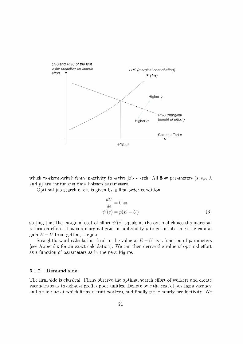
Optimal job search e�ort is given by a �rst order condition:

dU

de= 0⇔

ψ′(e) = p(E − U) (3)

stating that the marginal cost of e�ort ψ′(e) equals at the optimal choice the marginalreturn on e�ort, that is a marginal gain in probability p to get a job times the capitalgain E − U from getting the job.

Straightforward calculations lead to the value of E − U as a function of parameters(see Appendix for an exact calculation). We can then derive the value of optimal e�ortas a function of parameters as in the next Figure.

5.1.2 Demand side

The �rm side is classical. Firms observe the optimal search e�ort of workers and createvacancies so as to exhaust pro�t opportunities. Denote by c the cost of posting a vacancyand q the rate at which �rms recruit workers, and �nally y the hourly productivity. We

21

have :

rV = −c+ q(J − V )

rJ = yh− wh+ (s+ sN)(V − J)

where V is the value of a job vacancy and J is the value of a �lled job. Free-entry impliesthat

V = 0

=⇒ J = c/q =yh− whr + s+ sN

5.1.3 Equilibrium

Finally, both p and q are made consistent through the existence of an aggregate matchingfunction M(eNU , NV ) where NU is the number of unemployed, e is the average jobsearch e�ort in the population of the unemployed, and NV is the number of postedvacancies. We assume a constant return to scale function. Hence we have, introducingθ = NV

eNU, the following transition rates:

p =M(eNU , NV )

eNU

= M(1, θ) = p(θ)

q =M(eNU , NV )

NV

= M(1/θ, 1) = q(θ)

with p′(θ) > 0 and q′(θ) < 0.

This delivers the equilibrium value of θ, since there is a unique θ∗ function of theparameters y, w, c, r, s and sN such that

c

q(θ∗)=

yh− whr + s+ sN

Plugging into the optimal search e�ort condition determined by equation (3), weobtain the optimal search e�ort e∗(α, p(θ∗)). The equilibrium of the labor market istherefore described by the couple (θ∗, e∗).

22

Proposition 1 Labor market tightness does not depend on α, the level of RMI as com-pared to the minimum wage. The RMI has an impact only through a reduction in jobsearch e�ort e∗, with ∂e∗

∂α< 0.

Firms react to RMI through the search e�ort: the value of θ∗ is independent of α,but the total number of vacancies is equal to NV = e∗ × θ∗ and thus reacts to the RMI.

In a symmetric equilibrium where every unemployed individual searches the sameamount, we have the following stock-�ow conditions :

dNU

dt= 0 = λNN + s(1−NN −NU)− e∗p(θ∗)NU

dNN

dt= 0 = −λNN + sN(1−NN −NU)

where 1 − NN − NU is the total number of jobs created by �rms. The last equationimplies that

NU = 1−NN(1 +λ

sN)

while the �rst one implies

λNN(1 +s

sN) = e∗p(θ∗)NU

Combining the two, we have

NU =1

1 + e∗p(θ∗)λ

sN+λsN+s

The number of unemployed workers decreases with θ∗ and with job search e�ort andincreases with s.

Proposition 2 Denote by e∗0 the value of job search e�ort when α = 0 (no RMI),and by e∗(α) the post-RMI value as calculated above. The causal impact of RMI onunemployment is given by

Λ =1

1 + e∗(α)p(θ∗)λ

sN+λsN+s

− 1

1 +e∗0p(θ

∗)

λsN+λsN+s

23

Corollary 3 The rate of unemployment is

u = NU/(1−NN) =1

1 + e∗(α)ps+sN

which increases with the out�ows from employment (s and sN), decreases with job searche�ort e∗and with the rate of job creation by �rms p(θ∗).

5.2 Extensions

5.2.1 Endogenous wage

Let us now assume that wages are not �xed but partly re�ect the workers' outsideoptions. To simplify, we assume a static bargaining rule, such that

wh = βyh+ (1− β)wR

where wR is the monthly wage that equalizes the utility νU and νE, namely

wR = rmi(0)− rmi(h) + ψ(h)− ψ(e)

Given that rmi(0) − rmi(h) is greater than 0 for all hours worked, the introduction ofthe RMI must raise wages in the economy for all eligible workers except when β is equalto one.

5.2.2 Job search

A second extension is to allow individuals to direct their search towards either part-time or full-time jobs. Indeed, many of the RMI recipients were not able to immediatelyobtain a full time job and had to accept, at least for some time, part-time jobs where thedisincentive e�ects of RMI were likely to be large. Therefore, we may want to modifythe model to allow for this possibility. Relaxing �rst the labor demand side, we candecompose the search e�ort into two components, e = eF + eP where the subscript F,P re�ect the e�ort spent into full-time or part-time. Similarly let pF and pP be the job�nding rate of part-time and full-time jobs. Finally, let E(P ) and E(F ) be the value ofpart-time and full time employment. We have

rU = rmi(0)− ψ(eF + eP ) + (pF × eF )(EF − U) + (pP × eP )(EP − U).

24

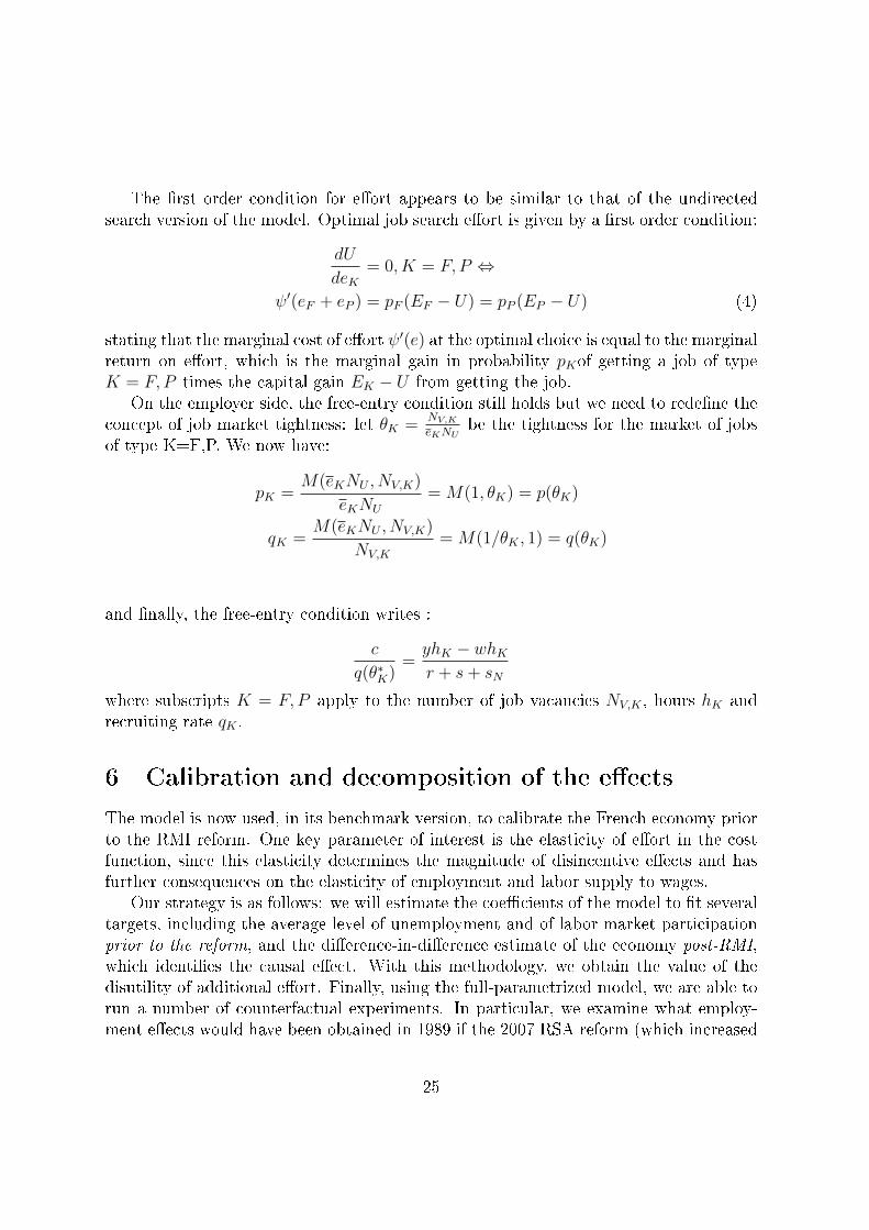
The �rst order condition for e�ort appears to be similar to that of the undirectedsearch version of the model. Optimal job search e�ort is given by a �rst order condition:

dU

deK= 0, K = F, P ⇔

ψ′(eF + eP ) = pF (EF − U) = pP (EP − U) (4)

stating that the marginal cost of e�ort ψ′(e) at the optimal choice is equal to the marginalreturn on e�ort, which is the marginal gain in probability pKof getting a job of typeK = F, P times the capital gain EK − U from getting the job.

On the employer side, the free-entry condition still holds but we need to rede�ne theconcept of job market tightness: let θK =

NV,KeKNU

be the tightness for the market of jobsof type K=F,P. We now have:

pK =M(eKNU , NV,K)

eKNU

= M(1, θK) = p(θK)

qK =M(eKNU , NV,K)

NV,K

= M(1/θK , 1) = q(θK)

and �nally, the free-entry condition writes :

c

q(θ∗K)=yhK − whKr + s+ sN

where subscripts K = F, P apply to the number of job vacancies NV,K , hours hK andrecruiting rate qK .

6 Calibration and decomposition of the e�ects

The model is now used, in its benchmark version, to calibrate the French economy priorto the RMI reform. One key parameter of interest is the elasticity of e�ort in the costfunction, since this elasticity determines the magnitude of disincentive e�ects and hasfurther consequences on the elasticity of employment and labor supply to wages.

Our strategy is as follows: we will estimate the coe�cients of the model to �t severaltargets, including the average level of unemployment and of labor market participationprior to the reform, and the di�erence-in-di�erence estimate of the economy post-RMI,which identi�es the causal e�ect. With this methodology, we obtain the value of thedisutility of additional e�ort. Finally, using the full-parametrized model, we are able torun a number of counterfactual experiments. In particular, we examine what employ-ment e�ects would have been obtained in 1989 if the 2007 RSA reform (which increased

25

the incentives to work when compared with the RMI alone) had been implemented rightaway, in place of the RMI.

The calibration speci�cally targets a group of unskilled workers over the period 1982-1988, chosen among those most likely to be paid around the minimum wage level andto potentially be eligible for the RMI. The target group is chosen among the 25-55 yearold population, so as to remove transitions between higher education and activity orbetween activity and retirement. We also select those having an education level below"Baccalauréat", that is the equivalent of high school dropouts. Summary statistics ofthis population group are displayed in Appendix Table 1.

We see that 81 percent of them are either employed or unemployed. Those with ajob have on average a wage equal to 124% of the minimum wage23. The fraction of theunemployed population amounts to 10 percent of the labor force. The six transitionsbetween the three di�erent labor market states E, U and N are displayed in the bottom ofthe table. The high school dropouts represent 63% of the 25-55 year old. The statisticsare reported in Table Appendix 1.

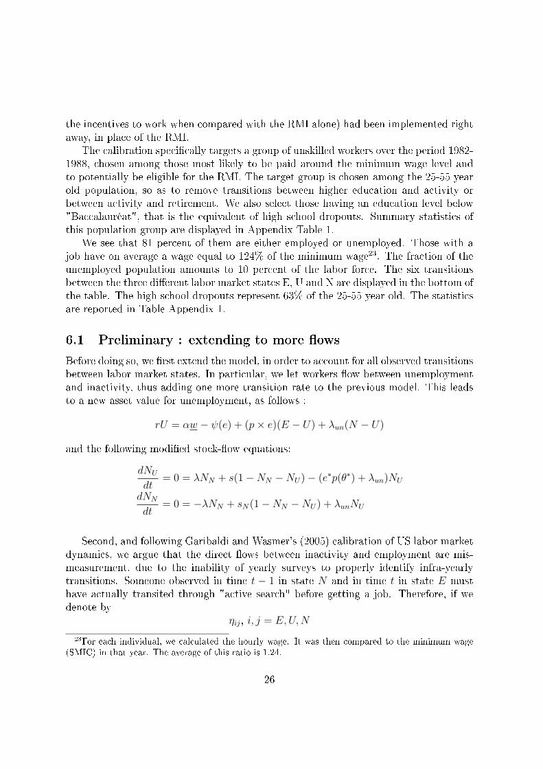
6.1 Preliminary : extending to more �ows

Before doing so, we �rst extend the model, in order to account for all observed transitionsbetween labor market states. In particular, we let workers �ow between unemploymentand inactivity, thus adding one more transition rate to the previous model. This leadsto a new asset value for unemployment, as follows :

rU = αw − ψ(e) + (p× e)(E − U) + λun(N − U)

and the following modi�ed stock-�ow equations:

dNU

dt= 0 = λNN + s(1−NN −NU)− (e∗p(θ∗) + λun)NU

dNN

dt= 0 = −λNN + sN(1−NN −NU) + λunNU

Second, and following Garibaldi and Wasmer's (2005) calibration of US labor marketdynamics, we argue that the direct �ows between inactivity and employment are mis-measurement, due to the inability of yearly surveys to properly identify infra-yearlytransitions. Someone observed in time t − 1 in state N and in time t in state E musthave actually transited through "active search" before getting a job. Therefore, if wedenote by

ηij, i, j = E,U,N

23For each individual, we calculated the hourly wage. It was then compared to the minimum wage(SMIC) in that year. The average of this ratio is 1.24.

26

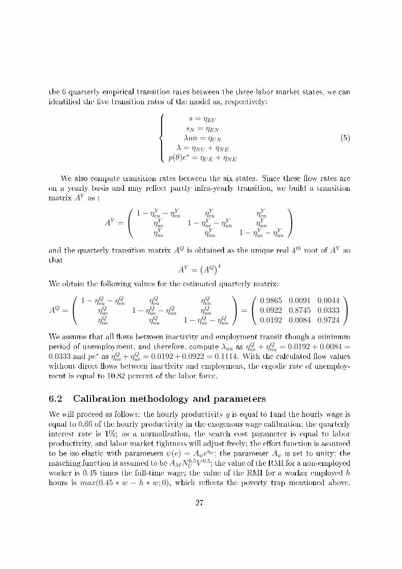
the 6 quarterly empirical transition rates between the three labor market states, we canidenti�ed the �ve transition rates of the model as, respectively:

s = ηEUsN = ηENλun = ηUN

λ = ηNU + ηNEp(θ)e∗ = ηUE + ηNE

(5)

We also compute transition rates between the six states. Since these �ow rates areon a yearly basis and may re�ect partly infra-yearly transition, we build a transitionmatrix AY as :

AY =

1− ηYeu − ηYen ηYeu ηYenηYue 1− ηYue − ηYun ηYunηYne ηYnu 1− ηYue − ηYun

and the quarterly transition matrix AQ is obtained as the unique real 4th root of AY sothat

AY =(AQ)4

We obtain the following values for the estimated quarterly matrix:

AQ =

1− ηQeu − ηQen ηQeu ηQenηQue 1− ηQue − ηQun ηQunηQne ηQnu 1− ηQue − ηQun

=

0.9865 0.0091 0.00440.0922 0.8745 0.03330.0192 0.0084 0.9724

We assume that all �ows between inactivity and employment transit though a minimumperiod of unemployment, and therefore, compute λnu as ηQne + ηQnu = 0.0192 + 0.0084 =0.0333 and pe∗ as ηQne + ηQue = 0.0192 + 0.0922 = 0.1114. With the calculated �ow valueswithout direct �ows between inactivity and employment, the ergodic rate of unemploy-ment is equal to 10.82 percent of the labor force.

6.2 Calibration methodology and parameters

We will proceed as follows: the hourly productivity y is equal to 1and the hourly wage isequal to 0.66 of the hourly productivity in the exogenous wage calibration; the quarterlyinterest rate is 1%; as a normalization, the search cost parameter is equal to laborproductivity, and labor market tightness will adjust freely; the e�ort function is assumedto be iso-elastic with parameters ψ(e) = Aψe

ηψ ; the parameter Aψ is set to unity; thematching function is assumed to be AMN0.5

U V 0.5; the value of the RMI for a non-employedworker is 0.45 times the full-time wage; the value of the RMI for a worker employed hhours is max(0.45 ∗ w − h ∗ w; 0), which re�ects the poverty trap mentioned above.

27

Hours are set to the average working hours in the sample,31.5 hours (h=31.5/39=0.8077of full-time.)

The di�erence-in-di�erences estimates of previous section (Table 2, columns 1) indi-cates a decrease in the job �nding rate by 7 percentage points a year (divide by 4 for thequarterly values) due to the causal e�ect of the RMI. We then let the code search for thevalues of parameters AM , ηψ such that the model matches the value of unemploymentbefore the reform(10.3 in the absence of the RMI); a -10/4 quarterly decrease in the job�nding rate after the implementation of the RMI. 24

6.3 Calibration results

We �nd the following values of the parameters and endogenous variables, as reportedin Table 4. Columns (1) and (2) report the results obtained from the same program,which jointly determines the parameter values and endogenous variables before and afterthe introduction of the RMI. Column (3) reports the results of another program, theRSA program. The RSA program is a 2007 reform of the RMI which keeps the basecomponent: RSA at zero hours was equal to the value of the RMI at zero hours. Butthe RSA at a positive number hours provided additional income for hours worked suchthat the marginal tax rate for the working individual would be 38% and not 100%:RSA(h) = max(rmi(0)− h× w × 0.38, 0), while RMI(h) = max(rmi(0)− h× w, 0).

The �rst set of rows provides the values of the parameters: the number of hours as afraction of a full-time, the total wage and the various transfers, rmi(0) and rmi(h). Forthe average worker, the amount of hours worked is such that the RMI yields no furthertransfer. Under a di�erent policy scenario with h = 0.5, this is not the case. In contrast,the value of the RSA amounted to 0.094, arguably a sizeable fraction of the earnings.

The second set of rows in the table reports the calibrated parameters of interest. Inparticular, the elasticity of e�ort in the cost function is large (8.9). This will lead tothe disincentive e�ects described above. The third set of rows reports the e�ect of theRMI on the main variables. E�ort goes down with the RMI, as does employment andthe hazard rate of employment. In contrast, the RSA leads to higher e�ort relative tothe RMI and mitigates the reduction in employment. We �nd that the RMI leads to an

24More precisely, the code has to solve for three asset values of employment, unemployment andinactivity (v1-3), the value of θ and e before the reform (v4-5), AM , ηψ (v6-7), the number of employedworkers, of unemployed workers and of non-participants before the reform (v8-10), and the same en-dogenous variables after the reform : three asset values of employment, unemployment and inactivity(v11-13), the value of θ and e after the reform (v14-15), and the number of employed workers, of unem-ployed workers and of non-participants after the reform (v16-18). The code is perfectly identi�ed sincewe have three Bellman equations, one free-entry condition and one optimal e�ort condition, 2 equationsfor the steady-state stock of employment and unemployment and a third one for participation (1-thesum of the two previous ones) : this leads to a total of 8 equations multiplied by two, before and afterthe reform, that is 16), to which we add a target for unemployment before the reform (10.3) and atarget for the reduction in the job hazard rate from Table 2, column 1 (-0.07/4), a total of 18 equations.

28

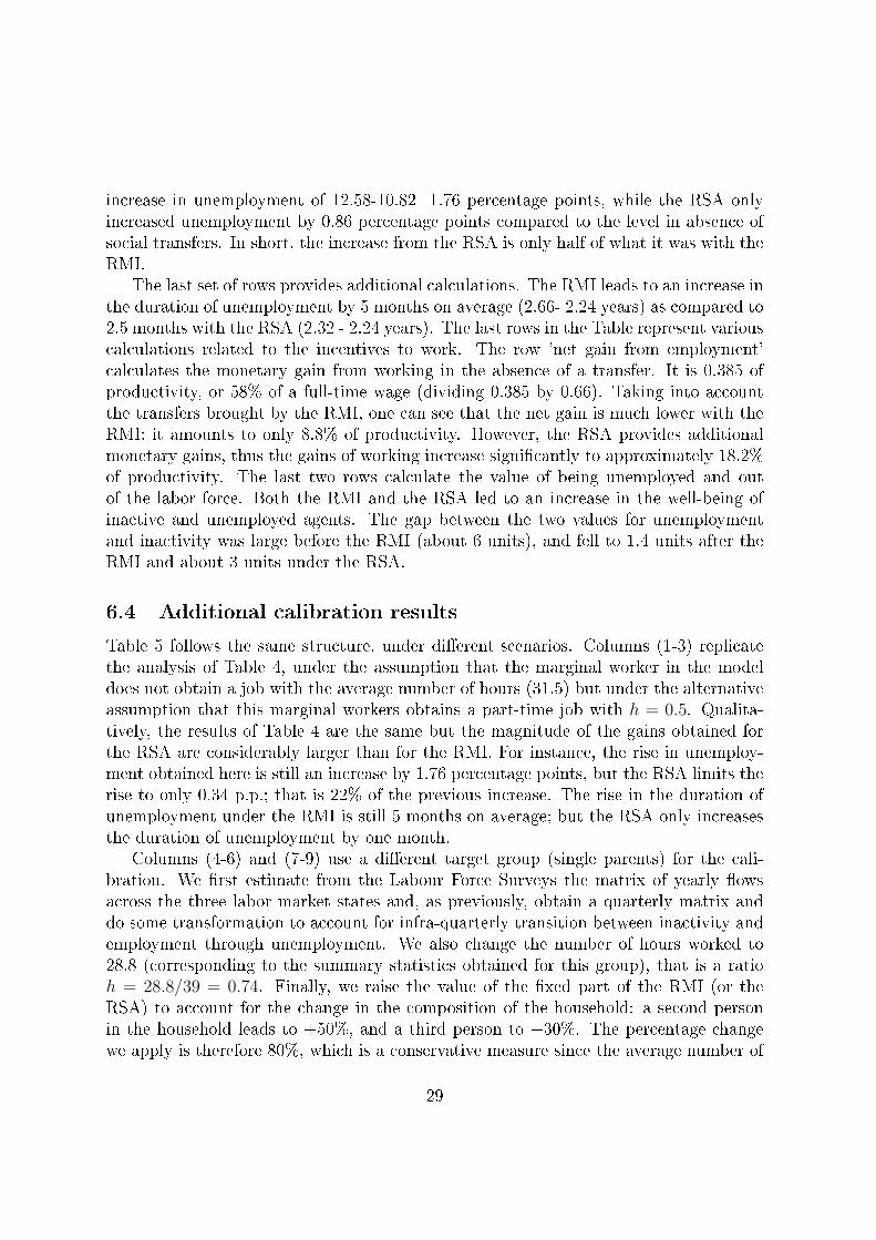
increase in unemployment of 12.58-10.82=1.76 percentage points, while the RSA onlyincreased unemployment by 0.86 percentage points compared to the level in absence ofsocial transfers. In short, the increase from the RSA is only half of what it was with theRMI.

The last set of rows provides additional calculations. The RMI leads to an increase inthe duration of unemployment by 5 months on average (2.66- 2.24 years) as compared to2.5 months with the RSA (2.32 - 2.24 years). The last rows in the Table represent variouscalculations related to the incentives to work. The row 'net gain from employment'calculates the monetary gain from working in the absence of a transfer. It is 0.385 ofproductivity, or 58% of a full-time wage (dividing 0.385 by 0.66). Taking into accountthe transfers brought by the RMI, one can see that the net gain is much lower with theRMI: it amounts to only 8.8% of productivity. However, the RSA provides additionalmonetary gains, thus the gains of working increase signi�cantly to approximately 18.2%of productivity. The last two rows calculate the value of being unemployed and outof the labor force. Both the RMI and the RSA led to an increase in the well-being ofinactive and unemployed agents. The gap between the two values for unemploymentand inactivity was large before the RMI (about 6 units), and fell to 1.4 units after theRMI and about 3 units under the RSA.

6.4 Additional calibration results

Table 5 follows the same structure, under di�erent scenarios. Columns (1-3) replicatethe analysis of Table 4, under the assumption that the marginal worker in the modeldoes not obtain a job with the average number of hours (31.5) but under the alternativeassumption that this marginal workers obtains a part-time job with h = 0.5. Qualita-tively, the results of Table 4 are the same but the magnitude of the gains obtained forthe RSA are considerably larger than for the RMI. For instance, the rise in unemploy-ment obtained here is still an increase by 1.76 percentage points, but the RSA limits therise to only 0.34 p.p.; that is 22% of the previous increase. The rise in the duration ofunemployment under the RMI is still 5 months on average; but the RSA only increasesthe duration of unemployment by one month.

Columns (4-6) and (7-9) use a di�erent target group (single parents) for the cali-bration. We �rst estimate from the Labour Force Surveys the matrix of yearly �owsacross the three labor market states and, as previously, obtain a quarterly matrix anddo some transformation to account for infra-quarterly transition between inactivity andemployment through unemployment. We also change the number of hours worked to28.8 (corresponding to the summary statistics obtained for this group), that is a ratioh = 28.8/39 = 0.74. Finally, we raise the value of the �xed part of the RMI (or theRSA) to account for the change in the composition of the household: a second personin the household leads to +50%, and a third person to +30%. The percentage changewe apply is therefore 80%, which is a conservative measure since the average number of

29

children of single parents is 2.87 in the sample. Unsurprisingly, the results are large andthe RMI has important disincentive e�ects for this category of workers, while the RSAleads to practically no change in the employment outcome. In columns (7) to (9), toisolate the e�ect of the additional income from RMI/RSA implied by the new householdcomposition from the e�ect of the di�erent elasticity of labor supply and the underlying�ows parameters, we run a counterfactual exercise in which we keep all values of theparameters except that of the RMI/RSA, which is kept to the value of a single adultwith no children. The impact of the RMI relative to the RSA is still di�erent; althoughthis is less notable than in columns (4) to (6).

7 Conclusion

Our paper uses an interesting natural experiment to obtain di�erence-in-di�erences esti-mates of the impact of French welfare reform. We �nd strong disincentive e�ects of theRMI. Using the di�erence-in-di�erences estimates, we then calibrate a model and assessthe e�ect of a major policy reform in 2007, the RSA, which provides additional incometo those who work without a�ecting the unemployed. We �nd that the disincentivee�ects are drastically reduced.

Our results are a �rst step toward integrating ex-post estimations of public policiesinto ex-ante structural approaches, a fruitful research direction proposed by Attanazioet al. (2003, 2009) and Todd and Wolpin (2009). This literature was developped toaddress a common criticism of ex-ante policy evaluations: that structural coe�cientsof interest may have changed after the reform due to general equilibrium e�ects. Inpart, our modelling strategy is immune to this critique. The estimates presented in ourcalibrations deal precisely with general equilibrium e�ects since our model allows for thefree entry of �rms. To account for general equilibrium e�ects, we calibrate our modelusing a di�erence-in-di�erences approach at the national level.

30

References

� Attanasio, Orazio, Costas Meghir and Ana Santiago, Education Choices in Mexico:Using a Structural Model and a Randomized Experiment to evaluate Progresa,mimeo UCL, �rst version 2001, last version 2009.

� Attanasio, Orazio, Costas Meghir and Miguel Skelezy. Using randomized experi-ments and structural models for `scaling up'. Evidence from PROGRESA evalua-tion, mimeo UCL, 2003.

� Behaghel L., B. Crépon et B. Sédillot (2004) : � Contribution Delalande et tran-sitions sur le marché du travail � , Economie et Statistiques.

� Bertrand, Marianne, Esther Du�o, and Sendhil Mullainathan. 2004. How MuchShould We Trust Di�erences-in-Di�erences Estimates? Quarterly Journal of Eco-nomics 119(1), 249-275.

� Blundell, R.W. and T. MaCurdy (1999): Labour Supply: A Review of AlternativeApproaches, in O. Ashenfelter and D. Card (eds): Handbook of Labor Economics,vol. 3A, 1559-1604.

� Chemin, Matthieu and Etienne Wasmer. 2009. Using Alsace-Moselle local lawsto build a di�erence-in-di�erence estimation strategy of the employment e�ects ofthe 35-hour workweek regulation in France, Journal of Labor Economics 27(4),487-524.

� Clément, Élise. 2009. Les dépenses d'aide sociale départementale en 2007. Étudeset Résultats, Direction de la recherche, des études, de l'évaluation et des statis-tiques (DREES), 682, mars 2009.

� Crépon B. and F. Kramarz (2002) : � Employed 40 Hours or Not employed 39: Lessons from the 1981 Mandatory Reduction of the weekly Working Hours �Journal of Political Economy

� Daniel, Christine. 1999. L'indemnisation du chômage depuis 1979: di�érenciationdes droits, éclatement des statuts. Revue de l'IRES n.29, hiver 1998-99, pp 5-28.

� Flinn, Christopher and Jim Heckman (1983). �Are Unemployment and Out-of-the-Labor-Force Behaviorally Distinct Labor Force States?,� Journal of Labor Eco-nomics 1 (January): 28-42.

� Fortin, Bernard, Lacroix, Guy, and Simon Drolet. (2004). �Welfare bene�ts andthe duration of welfare spells: evidence from a natural experiment in Canada�,Journal of Public Economics 88, 1495-1520.

31

� Fougere D. and L. Rioux. 2001. �Le RMI treize ans après : entre redistribution etincitations�, Economie et Statistique, n° 346-347, 2001, 3-12.

� Garibaldi P. and E. Wasmer 2005. "Equilibrium Search Unemployment, Endoge-nous Participation, And Labor Market Flows," Journal of the European EconomicAssociation, MIT Press, vol. 3(4), pages 851-882, 06.

� Gurgand M. and D. Margolis, 2001. �RMI et revenus du travail : une évaluationdes gains �nanciers à l'emploi�, Economie et Statistique, n° 346-347, 2001, 103-115

� Hagnéré C. and Trannoy, A. 2001. "The combined e�ect of three years of reformon the inactivity traps", Economie et Statistique, n° 346-347, 2001, 161-179.

� Jones Stephen R. G. & W. Craig Riddell (1999). "The Measurement of Unemploy-ment: An Empirical Approach," Econometrica, Econometric Society, vol. 67(1),pages 147-162, January.

� Lee, D., (2008), �Randomized experiments from non-random selection in U.S.House elections�, Journal of Econometrics, 142, p. 675-697.

� Lemieux, Thomas, and Kevin Milligan. 2008. �Incentive e�ects of social assistance:A regression discontinuity approach�, Journal of Econometrics 142, 807�828.

� L'Horty, Yannick and Antoine Parent. 1999. La revalorisation du RMI. Revueéconomique, 50(3), 465-478.

� Moulton, Brent. 1990. An Illustration of a Pitfall in Estimating the E�ects ofAggregate Variables on Micro Units, Review of Economics and Statistics 72(2),334-338.

� Piketty, T. (1998). �L'impact des incitations �nancières au travail sur les com-portements individuels: une estimation pour le cas français�, Report to the French�Commissariat Général au Plan�

� Pissarides (2000). Equilibrium Unemployment Theory, MIT Press.

� Rioux L. �Salaire de réserve, allocation chômage dégressive et revenu minimum�,Economie et Statistique, 346-347, 2001.

� Terracol, A. (2009). �Guaranteed minimum income and unemployment durationin France�, Labour Economics, volume 16, pages171-182, number 2

� Todd, Petra E. and Kenneth I. Wolpin. �Structural Estimation and Policy Evalu-ation in Developing Countries�, Penn Institute for Social Research 09-028

32

� Woehrling, Jean-Marie. 2002. Alsace-Moselle. Droit Communal Local. BiensCommunaux et Services Publics Communaux, Fascicule 224, Jurisclasseur Alsace-Moselle.

� Zoyem, J.P. (2001), �Contrats d'insertion et sortie du RMI�, Economie et Statis-tique, n° 346-347.

33

Table

1:Im

pactoftheRMIontransitionsandstocks

(samplerestricted

tothe25-55years

old)

(1)

(2)

(3)

(4)

(5)

(6)

(7)

(U+N)to

EUto

ENto

USearch

EU

Wage

Dependentvariable

1ifE,0otherwise

1ifE,0otherwise

1ifU,0otherwise

Searche�ort

1ifE,0otherwise

1ifU,0otherwise

Wage

Sample

Longterm

UorN

Longterm

UN

Longterm

UUnskilled(H

ighschooldropouts)

Low

incomehh

Low

incomehh

Low

incomehh

Low

incomehh

ayearbefore

ayearbefore

ayearbefore

ayearbefore

RestofFrance*After

year1989

-0.04

-0.12

0.009

-0.09

-0.04

0.02

133.57

(8.41)***

(4.88)***

(1.24)

(1.62)

(5.50)***

(1.96)*

(0.73)

Departem

ent�xed

e�ects

Yes

Yes

Yes

Yes

Yes

Yes

Yes

Year�xed

e�ects

Yes

Yes

Yes

Yes

Yes

Yes

Yes

Controlvariables

Yes

Yes

Yes

Yes

Yes

Yes

Yes

Observationsi

44663

6074

34978

6074

493795

493795

371444

R-squared

0.03

0.05

0.03

0.02

0.15

0.02

0.04

OLSregressions.Robusttstatisticsin

parentheses,clustered

atthelevelofdepartem

ent.*signi�cantat10%;**signi�cantat5%;***signi�cantat1%.Thesample

isrestricted

tothose

25-55years

old.Thedependentvariablein

column(1)isadichotomousvariable,equalto

"1"iftheindividualisworking,"0"otherwise.

The

samplein

columns(1)isrestricted

tothelong-term

(more

than20months)unem

ployedin

alowincomehousehold

ayearbefore.Theseindividualsare

eligibleforthe

RMIin

thecurrentyearofobservationifthey

remain

unem

ployed.Theexplanatory

variableofinterestis"RestOfFrance*After

year1989",theinteractionbetweena

dichotomousvariableequalto

"1"iftheindividualresides

intheRestofFrance,"0"ifheresides

inAlsace-M

oselle,andaseconddichotomousvariableequalto

"1"if

theobservationisafter

theyear1989,"0"otherwise.

Thecontrolvariablesin

allcolumnsinclude�veagedummies,thesexoftheindividual,thehousehold

size,and

15educationdummies.

95departem

ent�xed

e�ects,andyear�xed

e�ects

are

alsoincluded

inallcolumns.

Columns(1),(2)and(3)lookattransitionsfrom

(U+N)

toE,U

toE,andN

toU.Thedependentvariablein

column(4)isthechange,from

oneyearto

thenext,in

adichotomousvariable,equalto

"1"iftheindividual

hasplacedanadorresponded

toanadin

anew

spaper

oronanotice-board.Thesamplein

column(4)isthelong-term

(more

than20months)unem

ployed

inalow

incomehousehold

ayearbefore.Columns(5)and(6)lookatthestocksofem

ployedandunem

ployed.Thedependentvariablein

column(7)isthewage.

Incolumns

(5),(6),and(7),thesampleisrestricted

totheunskilledworkers(highschooldropouts).

34

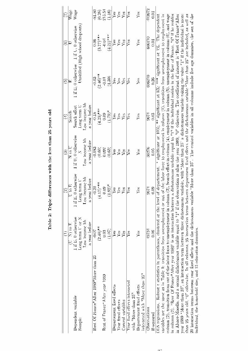
Table

2:Triple

di�erenceswiththeless

than25years

old

(1)

(2)

(3)

(4)

(5)

(6)

(7)

(U+N)to

EUto

ENto

USearch

EU

Wage

Dependentvariable

1ifE,0otherwise

1ifE,0otherwise

1ifU,0otherwise

Searche�ort

1ifE,0otherwise

1ifU,0otherwise

Wage

Sample

Longterm

UorN

Longterm

UN

Longterm

UUnskilled(H

ighschooldropouts)

Low

incomehh

Low

incomehh

Low

incomehh

Low

incomehh

ayearbefore

ayearbefore

ayearbefore

ayearbefore

RestOfFrance*After

1989*More

than25

-0.07

-0.20

-0.083

-0.18

-0.03

0.06

-81.80

(2.48)**

(4.17)***

(0.60)

(4.23)***

(2.46)**

(3.77)***

(0.28)

RestofFrance*After

year1989

0.03

0.09

0.092

0.09

-0.01

-0.04

215.54

(1.07)

(1.92)*

(0.63)

(1.79)*

(1.39)

(4.21)***

(1.16)

Departem

ent�xed

e�ects

Yes

Yes

Yes

Yes

Yes

Yes

Yes

Year�xed

e�ects

Yes

Yes

Yes

Yes

Yes

Yes

Yes

Controlvariables

Yes

Yes

Yes

Yes

Yes

Yes

Yes

Year�xed

e�ectsinteracted

Yes

Yes

Yes

Yes

Yes

Yes

Yes

with"More

than25"

Departem

ent�xed

e�ects

Yes

Yes

Yes

Yes

Yes

Yes

Yes

interacted

with"More

than25"

Observations

49734

9674

36276

9674

606210

606210

412672

R-squared

0.06

0.09

0.05

0.03

0.26

0.04

0.04

OLSregressions.

Robust

tstatisticsin

parentheses,clustered

atthelevelofdepartem

ent.

*signi�cantat10%;**signi�cantat5%;***signi�cantat1%.Thedependent

variablesare

thesameasin

Table1:transitionfrom

unem

ploymentoroutofthelaborforceto

employmentin

column(1),transitionfrom

unem

ploymentto

employmentin

column(2),transitionfromoutofthelaborforceto

unem

ploymentincolumn(3),Searche�ortincolumn(4),em

ploymentincolumn(5),unem

ploymentincolumn(6),andwage

incolumn(7).

�RestOfFrance*After

year1989�isaninteractionbetweenadichotomousvariableequalto

"1"iftheindividualresides

intheRestofFrance,"0"ifheresides

inAlsace-M

oselle,andaseconddichotomousvariableequalto

"1"iftheobservationisafter

theyear1989,"0"otherwise.

Thecoe�

cientofinterest

is�R

estOfFrance*After

year1989*More

than25�,aninteractionterm

betweenthreedichotomousvariable,with�M

ore

than25�adichotomousvariabletakingthevalue"1"iftheindividualismore

than25years

old,�0�otherwise.

Inallcolumns,95interactionterm

sbetweendepartment�xed

e�ects

andthedichotomousvariable�M

ore

than25�are

included,aswellas

20interactionterm

sbetweenyear�xed

e�ects

andthedichotomousvariable

�More

than25�.

Thecontrolvariablesin

allcolumnsinclude�veagedummies,thesexofthe

individual,thehousehold

size,and15educationdummies.

35

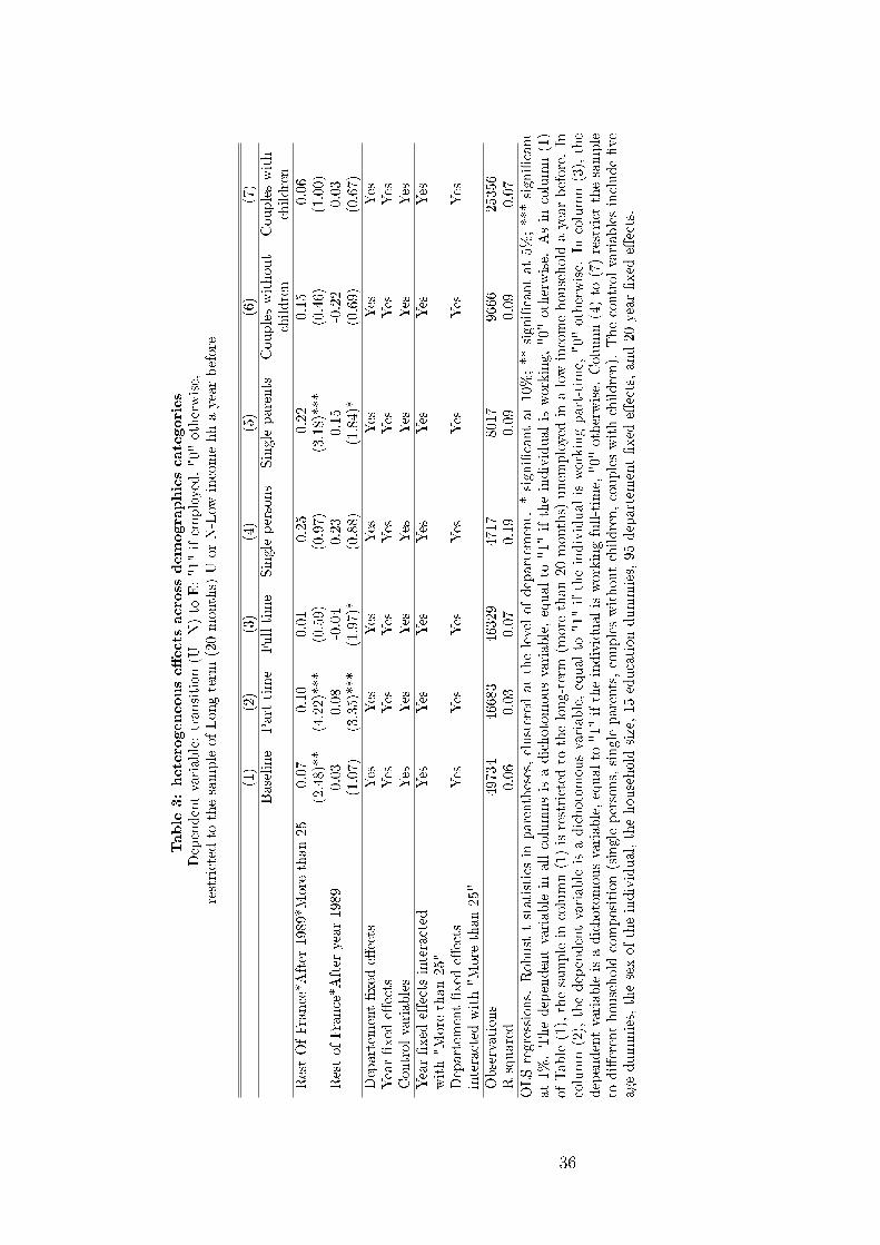
Table

3:heterogeneouse�ects

across

demographicscategories

Dependentvariable:transition(U

+N)to

E:"1"ifem

ployed,"0"otherwise,

restricted

tothesampleofLongterm

(20months)UorN-Low

incomehhayearbefore

(1)

(2)

(3)

(4)

(5)

(6)

(7)

Baseline

Parttime

Fulltime

Singlepersons

Singleparents

Coupleswithout

Coupleswith

children

children

RestOfFrance*After

1989*More

than25

-0.07

-0.10

0.01

-0.25

-0.22

0.15

-0.06

(2.48)**

(4.22)***

(0.59)

(0.97)

(3.18)***

(0.46)

(1.00)

RestofFrance*After

year1989

0.03

0.08

-0.04

0.23

0.15

-0.22

0.03

(1.07)

(3.35)***

(1.97)*

(0.88)

(1.84)*

(0.69)

(0.67)

Departem

ent�xed

e�ects

Yes

Yes

Yes

Yes

Yes

Yes

Yes

Year�xed

e�ects

Yes

Yes

Yes

Yes

Yes

Yes

Yes

Controlvariables

Yes

Yes

Yes

Yes

Yes

Yes

Yes

Year�xed

e�ectsinteracted

Yes

Yes

Yes

Yes

Yes

Yes

Yes

with"More

than25"

Departem

ent�xed

e�ects

Yes

Yes

Yes

Yes

Yes

Yes

Yes

interacted

with"More

than25"

Observations

49734

46683

46329

4717

8017

9666

25356

R-squared

0.06

0.03

0.07

0.19

0.09

0.09

0.07

OLSregressions.

Robust

tstatisticsin

parentheses,clustered

atthelevelofdepartem

ent.

*signi�cantat10%;**signi�cantat5%;***signi�cant

at1%.Thedependentvariablein

allcolumnsisadichotomousvariable,equalto

"1"iftheindividualisworking,"0"

otherwise.

Asin

column(1)

ofTable(1),thesamplein

column(1)isrestricted

tothelong-term

(more

than20months)

unem

ployedin

alowincomehousehold

ayearbefore.In

column(2),thedependentvariableisadichotomousvariable,equalto

"1"iftheindividualisworkingpart-time,"0"otherwise.

Incolumn(3),the

dependentvariableisadichotomousvariable,equalto

"1"iftheindividualisworkingfull-time,"0"otherwise.

Column(4)to

(7)restrict

thesample

todi�erenthousehold

composition(singlepersons,singleparents,coupleswithoutchildren,coupleswithchildren).

Thecontrolvariablesinclude�ve

agedummies,thesexoftheindividual,thehousehold

size,15educationdummies,95departem

ent�xed

e�ects,and20year�xed

e�ects.

36

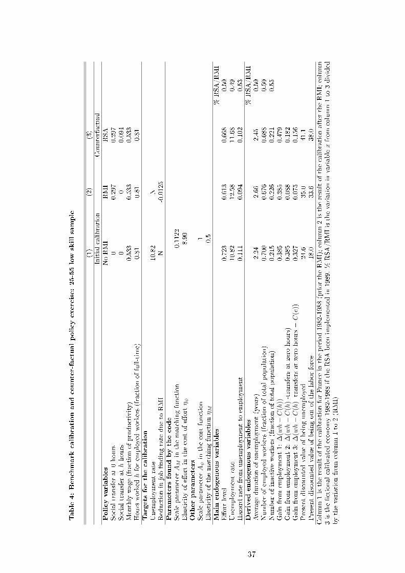
Table

4:Benchmark

calibrationandcounter-factualpolicyexercise:25-55lowskillsample

(1)

(2)

(3)

Initialcalibration

Counterfactual

Policyvariables

NoRMI

RMI

RSA

Socialtransfer

at0hours

00.297

0.297

Socialtransfer

athhours

00

0.094

Monthly

wage(fractionofproductivity)

0.533

0.533

0.533

Hoursworkedhforem

ployed

workers(fractionoffull-time)

0.81

0.81

0.81

Targets

forthecalibration

Unem

ploymentrate

10.82

NReductionin

job�ndingrate

dueto

RMI

N-0.0125

Parameters

foundbythecode

ScaleparameterAM

inthematchingfunction

0.1122

Elasticityofe�ortin

thecostofe�ortη ψ

8.90

Otherparameters

ScaleparameterAψin

thecostfunction

1Elasticityofthematchingfunctionη M

0.5

Main

endogenousvariables

%RSA/RMI

E�ortlevel

0.723

0.613

0.668

0.50

Unem

ploymentrate

10.82

12.58

11.68

0.49

Hazard

rate

from

unem

ploymentto

employment

0.111

0.094

0.102

0.53

Derivedendogenousvariables

%RSA/RMI

Averagedurationofunem

ployment(years)

2.24

2.66

2.45

0.50

Number

ofem

ployedworkers(fractionoftotalpopulation)

0.700

0.676

0.688

0.50

Number

ofinactiveworkers(fractionoftotalpopulation)

0.215

0.226

0.221

0.55

Gain

from

employment1:

∆(wh−C

(h))

0.385

0.385

0.479

Gain

from

employment2:

∆(wh−C

(h)-transfersatzero

hours)

0.385

0.088

0.182

Gain

from

employment3:

∆(wh−C

(h)-transfersatzero

hours+C

(e))

0.327

0.075

0.156

Presentdiscountedvalueofbeingunem

ployed

24.6

35.0

41.1

Presentdiscountedvalueofbeingoutofthelaborforce

18.0

33.6

38.0

Column1istheresultofthecalibrationforFrance

intheperiod1982-1988(priortheRMI);column2istheresultofthecalibrationafter

theRMI;column

3isthe�ctionalcalibratedeconomy1982-1988iftheRSAbeenimplementedin

1989.%

RSA/RMIisthevariationin

variablexfrom

column1to

3divided

bythevariationfrom

column1to

2(R

MI)

37

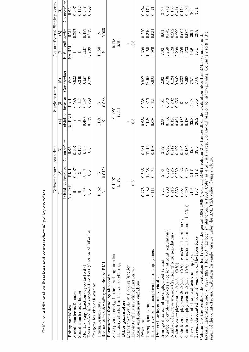
Table

5:Additionalcalibrationsandcounter-factualpolicyexercises Di�erenthours:part-time

Singleparents

CounterfactualSingleparents

(1)

(2)

(3)

(4)

(5)

(6)

(7)

(8)

(9)

Initialcalibration

Counterfact.

Initialcalibration

Counterfact.

Initialcalibration

Counterfact.

Policyvariables

NoRMI

RMI

RSA

NoRMI

RMI

RSA

NoRMI

RMI

RSA

Socialtransfer

at0hours

00.297

0.297

00.535

0.535

00.297

0.297

Socialtransfer

athhours

00

0.176

00.047

0.349

00

0.112

Monthly

wage(fractionofproductivity)

0.33

0.33

0.33

0.487

0.487

0.487

0.487

0.487

0.487

Hoursworkedhforem

ployed

workers(fractionoffull-time)

0.5

0.5

0.5

0.739

0.739

0.739

0.739

0.739

0.739

Targets

forthecalibration

Unem

ploymentrate

10.82

N14.50

N14.50

NReductionin

job�ndingrate

dueto

RMI

N-0.0125

N-0.055

N-0.055

Parameters

foundbythecode

ScaleparameterAM

inthematchingfunction

0.1407

0.0951

0.118

Elasticityofe�ortin

thecostofe�ortη ψ

13.78

72.14

5.50

Otherparameters

ScaleparameterAψin

thecostfunction

11

1Elasticityofthematchingfunctionη M

0.5

0.5

0.5

Main

endogenousvariables

E�ortlevel

0.778

0.656

0.751

0.934

0.338

0.927

0.609

0.220

0.504

Unem

ploymentrate

10.82

12.58

11.16

14.50

0.319

14.58

14.50

0.319

0.170

Hazard

rate

from

unem

ploymentto

employment

0.111

0.094

0.108

0.086

0.031

0.085

0.086

0.031

0.071

Derivedendogenousvariables

Averagedurationofunem

ployment(years)

2.24

2.66

2.32

2.90

8.01

2.92

2.90

8.01

3.50

Number

ofem

ployedworkers(fractionoftotalpopulation)

0.700

0.676

0.695

0.750

0.543

0.748

0.750

0.543

0.718

Number

ofinactiveworkers(fractionoftotalpopulation)

0.215

0.226

0.217

0.123

0.202

0.124

0.123

0.202

0.136

Gain

from

employment1:

∆(wh−C

(h))

0.330

0.330

0.502

0.487

0.535

0.837

0.299

0.299

0.411

Gain

from

employment2:

∆(wh−C

(h)-transfersatzero

hours)

0.384

0.033

0.205

0.487

00.302

0.299

0.002

0.114

Gain

from

employment3:

∆(wh−C

(h)-transfersatzero

hours+C

(e))

0.299

0.030

0.185

0.480

00.298

0.233

0.002

0.090

Presentdiscountedvalueofbeingunem

ployed

21.3

31.7

42.8

32.8

53.5

73.7

18.9

29.7

36.4

Presentdiscountedvalueofbeingoutofthelaborforce

15.7

31.2

39.3

26.2

53.5

70.0

15.1

29.8

35.1

Column1istheresultofthecalibrationforFrance

intheperiod1982-1988(priortheRMI);column2istheresultofthecalibrationafter

theRMI;column3isthe

�ctionalcalibratedeconomy1982-1988iftheRSAhadbeenimplementedin

1989.Columns4to

6istheresultofthecalibrationforsingleparents.Columns7to

9isthe

resultofthecounterfactualcalibrationforsingleparentsunder

theRMI/RSAvalueofsingleadults.

38

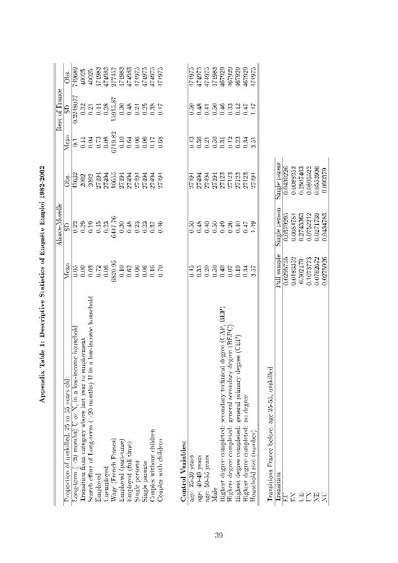
Appendix

Table

1:DescriptiveStatisticsofEnquête

Emploi1982-2002

Alsace-M

oselle

RestofFrance

Proportionofunskilled,25to

55years

old:

Mean

SD

Obs.

Mean

SD

Obs.

Long-term

(>20months)UorN,in

alow-incomehousehold

0.05

0.22

41632

0.1

0.2248077

749689

Transitionfrom

category

abovelastyearto

employment

0.09

0.29

2092

0.11

0.32

40025

Searche�ortofLong-term

(>20months)Uin

alow-incomehousehold

0.03

0.19

2092

0.04

0.21

40025

Employed

0.72

0.45

27494

0.73

0.44

474983

Unem

ployed

0.06

0.23

27494

0.08

0.28

474983

Wage(French

Francs)

6820.95

6447.76

16655

6719.82

15915.87

277457

Employed(part-time)

0.10

0.30

27494

0.10

0.30

474983

Employed(full-time)

0.62

0.48

27494

0.64

0.48

474983

Singlepersons

0.06

0.23

27494

0.06

0.24

474975

Singleparents

0.06

0.23

27494

0.06

0.25

474975

Coupleswithoutchildren

0.16

0.37

27494

0.17

0.38

474975

Coupleswithchildren

0.70

0.46

27494

0.68

0.47

474975

ControlVariables:

age:

25-39years

0.45

0.50

27494

0.43

0.50

474975

age:

40-49years

0.35

0.48

27494

0.36

0.48

474975

age:

50-55years

0.20

0.40

27494

0.21

0.41

474975

Male

0.50

0.50

27494

0.50

0.50

474983

Highestdegreecompleted:secondary

technicaldegree(CAP,BEP)

0.40

0.49

27123

0.31

0.46

467929

Highestdegreecompleted:generalsecondary

degree(BEPC)

0.07

0.26

27123

0.12

0.33

467929

Highestdegreecompleted:generalprimary

degree(CEP)

0.19

0.40

27123

0.23

0.42

467929

Highestdegreecompleted:nodegree

0.34

0.47

27123

0.34

0.47

467929

Household

size

(number)

3.57

1.49

27494

3.51

1.47

474975

TransitionsFrance

before,age25-55,unskilled

Transition

Fullsample

Singleperson

Singleparent

EU

0.0295755

0.0379295

0.0430226

EN

0.0183352

0.0084784

0.0088252

UE

0.302179

0.2743363

0.2507463

UN

0.1073773

0.0752212

0.0895522

NE

0.0762672

0.0271739

0.0553936

NU

0.0275926

0.0434783

0.090379

39

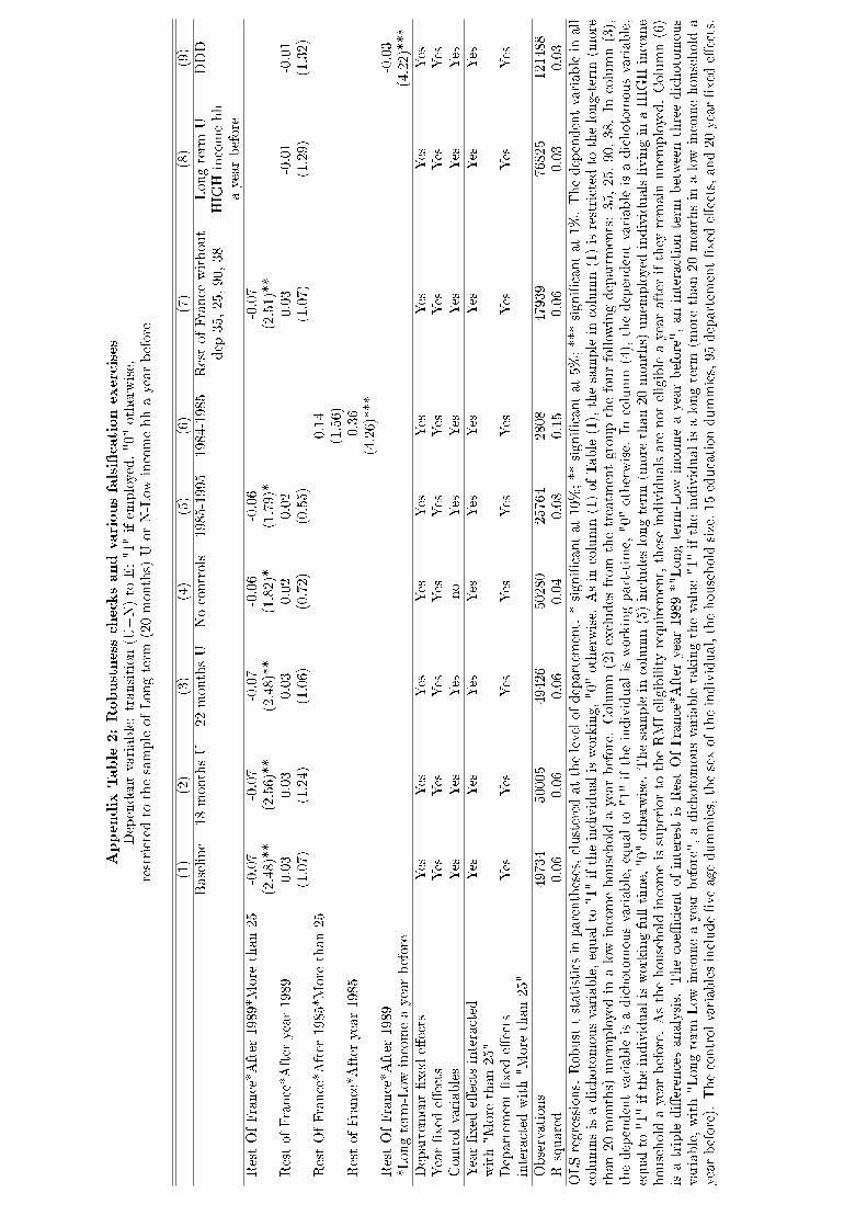
Appendix

Table

2:Robustness

checksandvariousfalsi�cationexercises

Dependentvariable:transition(U

+N)to

E:"1"ifem

ployed,"0"otherwise,

restricted

tothesampleofLongterm

(20months)UorN-Low

incomehhayearbefore

(1)

(2)

(3)

(4)

(5)

(6)

(7)

(8)

(9)

Baseline

18monthsU

22monthsU

Nocontrols

1985-1995

1984-1985

RestofFrance

without

Longterm

UDDD

dep

35,25,90,38

HIG

Hincomehh

ayearbefore

RestOfFrance*After

1989*More

than25

-0.07

-0.07

-0.07

-0.06

-0.06

-0.07

(2.48)**

(2.56)**

(2.48)**

(1.82)*

(1.79)*

(2.51)**

RestofFrance*After

year1989

0.03

0.03

0.03

0.02

0.02

0.03

-0.01

-0.01

(1.07)

(1.24)

(1.06)

(0.72)

(0.55)

(1.07)

(1.29)

(1.32)

RestOfFrance*After

1985*More

than25

0.14

(1.56)

RestofFrance*After

year1985

-0.36

(4.26)***

RestOfFrance*After

1989

-0.03

*Longterm

-Low

incomeayearbefore

(4.22)***

Departem

ent�xed

e�ects

Yes

Yes

Yes

Yes

Yes

Yes

Yes

Yes

Yes

Year�xed

e�ects

Yes

Yes

Yes

Yes

Yes

Yes

Yes

Yes

Yes

Controlvariables

Yes

Yes

Yes

no

Yes

Yes

Yes

Yes

Yes

Year�xed

e�ectsinteracted

Yes

Yes

Yes

Yes

Yes

Yes

Yes

Yes

Yes

with"More

than25"

Departem

ent�xed

e�ects

Yes

Yes

Yes

Yes

Yes

Yes

Yes

Yes

Yes

interacted

with"More

than25"

Observations

49734

50005

49426

50280

25764

2808

47939

76825

121488

R-squared

0.06

0.06

0.06

0.04

0.08

0.15

0.06

0.03

0.03

OLSregressions.Robusttstatisticsin

parentheses,clustered

atthelevelofdepartem

ent.*signi�cantat10%;**signi�cantat5%;***signi�cantat

1%.Thedependentvariablein

all

columnsisadichotomousvariable,equalto

"1"iftheindividualisworking,"0"otherwise.

Asin

column(1)ofTable(1),thesamplein

column(1)isrestricted

tothelong-term

(more

than20months)

unem

ployedin

alowincomehousehold

ayearbefore.Column(2)excludes

from

thetreatm

entgroupthefourfollow

ingdepartments:35,25,90,38.In

column(3),

thedependentvariableisadichotomousvariable,equalto

"1"iftheindividualisworkingpart-time,"0"otherwise.

Incolumn(4),thedependentvariableisadichotomousvariable,

equalto

"1"iftheindividualisworkingfull-time,"0"otherwise.

Thesamplein

column(5)includes

longterm

(more

than20months)unem

ployed

individualslivingin

aHIG

Hincome

household

ayearbefore.Asthehousehold

incomeissuperiorto

theRMIeligibilityrequirem

ent,theseindividualsare

noteligibleayearafter

ifthey

remain

unem

ployed.Column(6)

isatripledi�erencesanalysis.

Thecoe�

cientofinterest

isRestOfFrance*After

year1989*"Longterm

-Low

incomeayearbefore",aninteractionterm

betweenthreedichotomous

variable,with"Longterm

-Low

incomeayearbefore",adichotomousvariabletakingthevalue"1"iftheindividualisalongterm

(more

than20monthsin

alowincomehousehold

ayearbefore).Thecontrolvariablesinclude�ve

agedummies,thesexoftheindividual,thehousehold

size,15educationdummies,95

departem

ent�xed

e�ects,and20year�xed

e�ects.

40

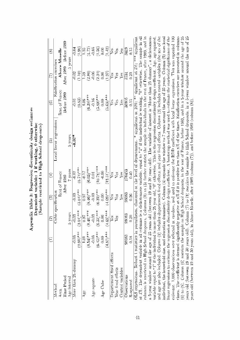
Appendix

Table

3:Regressiondiscontinuitydesignestim

ates

Dependentvariable:1ifworking,0otherw

ise

(Sample

restrictedto

HighSchooldrop-outs)

(1)

(2)

(3)

(4)

(5)

(6)

(7)

(8)

Method

Cubicspeci�cation

Locallinearregressions

Falsi�cationexercises

Area

RestofFrance

RestofFrance

AlsaceMoselle

TimePeriod

After

1989

Before

1989

After

1989

Before

1989

Ageinterval

5years

7years

5years

5years

More

than25dummy

-0.03

-0.03

-0.03

-0.07

-0.07*

-0.01

-0.02

-0.04

(2.91)***

(3.04)***

(3.04)***

(8.74)***

(0.83)

(1.10)

(1.90)

Age

1.01

0.97

0.97

-0.17

4.06

1.59

1.25

(8.54)***

(8.46)***

(8.46)***

(6.03)***

(6.20)***

(2.80)

(1.72)

Agesquare

-0.03

-0.03

-0.03

0.01

-0.16

-0.06

-0.05

(6.45)***

(6.32)***

(6.32)***

(10.78)***

(5.89)***

(2.34)

(1.56)

AgeCube

0.00

0.00

0.00

-0.00

0.00

0.00

0.00

(4.87)***

(4.69)***

(4.69)***

(13.51)***

(5.63)***

(1.97)

(1.43)

Departem

ent�xed

e�ects

Yes

Yes

Yes

Yes

Yes

Yes

Year�xed

e�ects

Yes

Yes

Yes

Yes

Yes

Yes

Controlvariables

Yes

Yes

Yes

Yes

Yes

Observations

98083

98083

98083

176453

36805

5731

3419

R-squared

0.18

0.20

0.26

0.40

0.15

0.23

0.15

OLSregressions.

Robust

tstatisticsin

parentheses,clustered

atthelevelofdepartem

ent.

*signi�cantat10%;**signi�cantat

5%;***signi�cant

at1%.Thedependentvariablein

allcolumnsisadichotomousvariable,equalto

"1"iftheindividualisworking,"0"otherwise.

Thesamplein

all

columnsisrestricted

toHighSchooldropouts.Columns(1)to

(3)further

restrict

thesampleto

individualsin

therest

ofFrance,after

1989,andin

a5-yearwindow

aroundtheageof25years

old

(between19and30years

old).

Thevariableofinterest

is�M

ore

than25dummy�,adichotomous

variableequalto

�1�iftheindividualismore

than25yearold,�0�otherwise.

Thisistheregressiondiscontinuitydesigncoe�

cient.Age,agesquared,

andageare

alsoincluded.Column(2)includes

departem

ent�xed

e�ects,andyear�xed

e�ects.Column(3)includes

controlvariables(thesexofthe

individual,thehousehold

size,andeducationdummies).Column(4)expandsthewindow

to7yearsaroundtheageof25years.Column(5)useslocal

linearregressionsto

estimate

theregressiondiscontinuitydesigncoe�

cient.Abootstrapmethodwasusedto

estimate

thestatisticalsigni�cance

ofthe

estimate.1,000observationswereselected

atrandom,andusedto

estimate

theRDDcoe�

cientwithlocallinearregressions.

Thiswasrepeated100

times.Thecoe�

cientisdeemed

signi�cantlynegative

atx%

ifitispositive

lessthanx%

ofthetimes.Falsi�cationexercisesare

presentedin

columns

(6)to

(8).

Column(6)restrictsthesampleto

HighSchooldropouts,in

therest

ofFrance,before

1989,andin

a5-yearwindow

aroundtheageof25

years

old

(between19and30years

old).

Column(7)to

(8)restrictsthesampleto

HighSchooldropouts,in

a5-yearwindow

aroundtheageof25

yearsold

(between19and30yearsold),in

Alsace-M

oselle,after

1989(column(7)),andbefore

1989

(column(8)).

41

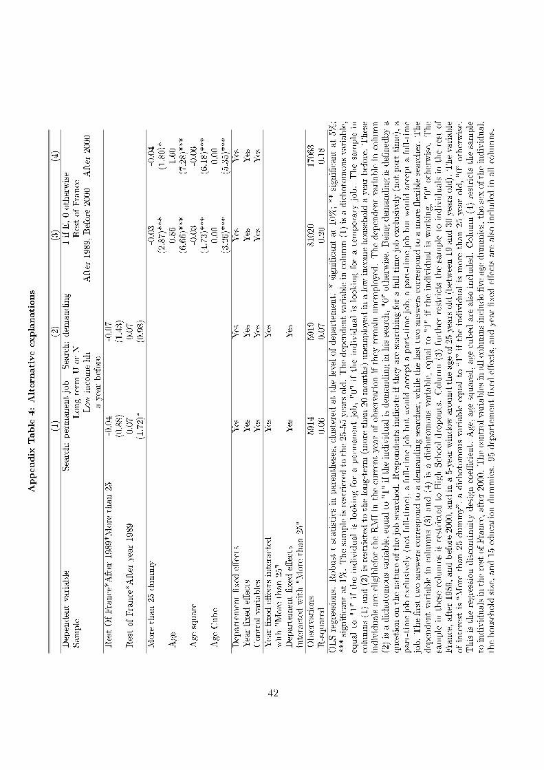
Appendix

Table

4:Alternativeexplanations

(1)

(2)

(3)

(4)

Dependentvariable

Search:permanentjob

Search:dem

anding

1ifE,0otherwise

Sample

Longterm

UorN

RestofFrance

Low

incomehh

After

1989,Before

2000

After

2000

ayearbefore

RestOfFrance*After

1989*More

than25

-0.04

-0.07

(0.88)

(1.43)

RestofFrance*After

year1989

0.07

0.07

(1.72)*

(0.98)

More

than25dummy

-0.03

-0.04

(2.87)***

(1.80)*

Age

0.86

1.60

(6.66)***

(7.28)***

Agesquare

-0.03

-0.06

(4.73)***

(6.18)***

AgeCube

0.00

0.00

(3.26)***

(5.35)***

Departem

ent�xed

e�ects

Yes

Yes

Yes

Yes

Year�xed

e�ects

Yes

Yes

Yes

Yes

Controlvariables

Yes

Yes

Yes

Yes

Year�xed

e�ectsinteracted

Yes

Yes

with"More

than25"

Departem

ent�xed

e�ects

Yes

Yes

interacted

with"Morethan25"

Observations

5914

5919

81020

17063

R-squared

0.06

0.07

0.20

0.18

OLSregressions.

Robust

tstatisticsin

parentheses,clustered

atthelevelofdepartem

ent.

*signi�cantat10%;**signi�cantat5%;

***signi�cantat1%.Thesampleisrestricted

tothe25-55yearsold.Thedependentvariablein

column(1)isadichotomousvariable,

equalto

"1"iftheindividualislookingforapermanentjob,"0"iftheindividualislookingforatemporary

job.Thesample

incolumns(1)and(2)isrestricted

tothelong-term

(more

than20months)unem

ployedin

alowincomehousehold

ayearbefore.

These

individualsare

eligiblefortheRMIin

thecurrentyearofobservation

ifthey

remain

unem

ployed.Thedependentvariablein

column

(2)isadichotomousvariable,equalto

"1"iftheindividualisdem

andingin

hissearch,"0"otherwise.

Beingdem

andingisde�nedbya

questiononthenature

ofthejobsearched.Respondentsindicate

ifthey

are

searchingforafull-timejobexclusively(notpart-time),a

part-timejobexclusively(notfull-time),afull-timejobbutwould

acceptapart-timejob,apart-timejobbutwould

acceptafull-time

job.The�rsttwoanswerscorrespondto

adem

andingsearcher,whilethelasttwoanswerscorrespondto

amore

�exiblesearcher.The

dependentvariablein

columns(3)and(4)isadichotomousvariable,equalto

"1"iftheindividualisworking,"0"otherwise.

The

samplein

thesecolumnsisrestricted

toHighSchooldropouts.Column(3)further

restrictsthesampleto

individualsin

therest

of

France,after1989,andbefore2000,andina5-yearwindow

aroundtheageof25yearsold(between19and30yearsold).Thevariable

ofinterest

is�M

ore

than25dummy�,adichotomousvariableequalto

�1�iftheindividual

ismore

than25yearold,�0�otherwise.

Thisistheregressiondiscontinuitydesigncoe�

cient.Age,agesquared,agecubed

are

alsoincluded.Column(4)restrictsthesample

toindividualsintherestofFrance,after

2000.Thecontrolvariablesinallcolumnsinclude�ve

agedummies,thesexoftheindividual,

thehousehold

size,and15educationdummies.95departem

ent�xed

e�ects,andyear�xed

e�ectsare

alsoincluded

inallcolumns.

42

Model Appendix

Bellman equations with full information

Starting from

rE = νe + s(U − E) + sN (N − E)

rU = νu + (p× e)(E − U)

rN = λ(U −N)

with

νe = hw + rmi(h)− ψ(h)

νu = rmi(0)− ψ(e)

we take the di�erence between the �rst and the second equation and between the �rst and the third,we obtain:

(r + s+ ep)(E − U) = νe − νu + sN (N − E)

(r + sN + λ)(E −N) = νe + (s− λ)(U − E)

Inserting E −N of the second equation into the �rst one, we have further:

(r + s+ ep)(E − U) = νe − νu+

sNr + sN + λ

[−νe + (s− λ)(E − U)]

or

E − U =r+λ

r+sN+λνe − νur + s+ ep+ sN

r+sN+λ (λ− s)(6)

Hence, the smaller the gap in income between employment and unemployment, the lower the gap

in asset values. In particular, the move from a situation where rmi(h) ≡ 0 for all hours to a situationwhere it is positive and decreasing in hours lead to a reduction in the di�erence between E and U .

Proof of Proposition 1, second part on e∗.Going back to the �rst order condition we have, replacing the value of (E − U) by that of equation

(6):

ψ′(e) = pr+λ

r+sN+λνe − νur + s+ ep+ sN

r+sN+λ (λ− s)(7)

The left-hand side is the marginal utility of leisure, it is thus increasing in e�ort e. The right handside is a decreasing function of e, moreover decreasing when rmi(.) is positive. Hence the proof of thesecond part of Proposition 1: there is a unique value of e�ort e∗ satisfying 7 and a shift in α reducessearch e�ort. See also Figure 5.1.1.

Stock-�ow equations with full information

Using the value of NU from the text, we can also compute NN . We have

NU =1

1 +A

NN =sN

λ+ sN

A

1 +A

43

where

A =e∗p

λ

λ+ sNs+ sN

Hence, the active population is

1−NN =λ+ sN

11+A

λ+ sN

and the rate of unemployment is

u =NU

1−NN=

1

1 + e∗p(θ∗)s+sN

Six-�ows ergodic unemployment rate

The ergodic unemployment rate is

dU/dt = E.ηeu +N.ηnu − U.(ηue + ηun) (8)

dE/dt = N.ηne + U.ηue − E.(ηeu + ηen) (9)

dN/dt = E.ηen + U.ηun −N.(ηne + ηnu) (10)

The stationary rate of unemployment is reached when E, N and U are constant: this is the rate ofunemployment corresponding to the ergodic distribution of workers in the three states.

De�nition 4 The ergodic rate of unemployment is given by:

u∗ =ηeu.ηne + ηeu.ηnu + ηen.ηnu

ηeu.ηne + ηeu.ηnu + ηen.ηnu + ηue.ηne + ηue.ηnu + ηne.ηun(11)

44