ARTICLE IN PRESS

Engineering Applications of Artificial Intelligence 22 (2009) 732–741

Contents lists available at ScienceDirect

Engineering Applications of Artificial Intelligence

0952-19

doi:10.1

Abbre

Artificia

Algorith

; BP, Ba� Corr

E-m

journal homepage: www.elsevier.com/locate/engappai

Evolutionary Artificial Neural Network Design and Trainingfor wood veneer classification

Marco Castellani a,�, Hefin Rowlands b

a Centro de Inteligencia Artificial (CENTRIA), Departamento Informatica, Universidade Nova Lisboa, 2829-516 Caparica, Portugalb Research & Enterprise Department, University of Wales, Newport, Allt-yr-yn Campus, PO Box 180, NP20 5XR Newport, UK

a r t i c l e i n f o

Article history:

Received 13 June 2006

Received in revised form

20 May 2008

Accepted 19 January 2009Available online 9 March 2009

Keywords:

Artificial Neural Networks

Evolutionary Algorithms

Artificial Neural Network Design

Pattern classification

Automated visual inspection

76/$ - see front matter & 2009 Elsevier Ltd. A

016/j.engappai.2009.01.013

vations: ANNGaT, Artificial Neural Network

l Neural Network; MLP, Multi-Layer Perceptr

m; GA, Genetic Algorithm; EP, Evolutionary P

ckpropagation; ANNT, Artificial Neural Netwo

esponding author. Tel.: +351 212948536; fax:

ail address: dr.caste@gmail.com (M. Castellan

a b s t r a c t

This study addresses the design and the training of a Multi-Layer Perceptron classifier for identification

of wood veneer defects from statistical features of wood sub-images. Previous research utilised a neural

network structure manually optimised using the Taguchi method with the connection weights trained

using the Backpropagation rule. The proposed approach uses the evolutionary Artificial Neural Network

Generation and Training (ANNGaT) algorithm to generate the neural network system. The algorithm

evolves simultaneously the neural network topology and the weights. ANNGaT optimises the size of the

hidden layer(s) of the neural network structure through genetic mutations of the individuals. The

number of hidden layers is a system parameter. Experimental tests show that ANNGaT produces highly

compact neural network structures capable of accurate and robust learning. The tests show no

differences in accuracy between neural network architectures using one and two hidden layers of

processing units. Compared to the manual approach, the evolutionary algorithm generates equally

performing solutions using considerably smaller architectures. Moreover, the proposed algorithm

requires a lower design effort since the process is fully automated.

& 2009 Elsevier Ltd. All rights reserved.

1. Introduction

Plywood is made of thin layers of wood, called veneers, joinedtogether using an adhesive. Defects of the veneer are identified byhuman inspectors as the sheets are transported to assembly on aconveyor. The task is extremely stressful and demanding andshort disturbances or loss of attention may result in mis-classification. Two distinct studies conducted on human inspec-tors in wood mills reported inspection accuracies ranging from amore optimistic 68% (Huber et al., 1985) estimate to a moreconservative 55% (Polzleitner and Schwingshakl, 1992) measure.

An automatic visual inspection system (Pham and Alcock,1996; Pham and Alcock, 1999a) was developed for this applicationby the Intelligent Systems Lab of the School of Engineering at theUniversity of Wales, Cardiff, UK and the Wood Research Instituteof Kuopio, Finland. Fig. 1 outlines the system. Monochromeimages of the veneer are pre-processed by automated algorithmsthat locate defect areas (Pham and Alcock, 1999b) where a set ofnumerical descriptors is extracted for further analysis. Seventeen

ll rights reserved.

Design and Training; ANN,

on; EA, Evolutionary

rogramming

rk Training

+351212948541.

i).

statistical attributes of the local grey level distribution wereidentified as relevant for defect identification (Lappalainen et al.,1994; Pham and Alcock, 1999c). Twelve possible defects of theveneer can be distinguished in contrast to clear wood giving 13possible classes. For each data sample, a classifier takes the 17-dimensional vector of image features and decides to which of the13 classes the pattern belongs.

Several algorithms were evaluated on their ability of correctlyrecognising wood veneer defects. The best results were obtainedusing an Artificial Neural Network (ANN) (Pham and Liu, 1995)classifier. In particular, Packianather (Packianather, 1997; Pack-ianather et al., 2000) reported 85% identification rates using athree-layered Multi-Layer Perceptron (MLP) (Pham and Liu, 1995).The accuracy result was substantially confirmed in an indepen-dent study by Pham and Sagiroglu (2000) using a four-layeredMLP classifier. Despite the similar classification accuraciesobtained, the conclusions of the two studies differed on the bestANN configuration.

This paper addresses the design of the MLP classifier system.To the present, ANN structure optimisation is still mainly a humanexpert’s job (Yao, 1999). Different ANN architectures are usuallytrained according to some pre-defined induction algorithm andtheir merit evaluated on the accuracy achieved. Unfortunately,training the frequently large set of parameters (i.e., the connectionweights) is one of the major problems in the implementation ofANN systems. Since most of ANN training procedures are based on

ARTICLE IN PRESS

Image segmentation

Image acquisition

Feature extraction

Classifier

CCD camera

veneer

Fig. 1. The AVI System.

Table 1Class distribution of wood veneer data set.

Class Number of examples

1 Bark 20

2 Clear wood 20

3 Coloured streaks 20

4 Curly grain 16

5 Discoloration 20

6 Holes 8

7 Pin knots 20

8 Rotten knots 20

9 Roughness 20

10 Sound knots 20

11 Splits 20

12 Streaks 20

13 Worm holes 8

Total examples 232

M. Castellani, H. Rowlands / Engineering Applications of Artificial Intelligence 22 (2009) 732–741 733

gradient descent of the error surface, they are prone to sub-optimal convergence to local minima. Such limitation in turnaffects the capability of precisely evaluating the ANN structures.A typical example of gradient-based learning algorithm is theBackpropagation (BP) rule (Rumelhart and McClelland, 1986) thatis used to train the MLP classifier of the automatic visualinspection system.

A growing number of literature reports efforts toward auto-matic design of ANN architectures (Branke, 1995; Yao, 1999).Constructive and destructive algorithms (LeCun et al., 1990; Reed,1993; Smieja, 1993) such as the Cascade Correlation LearningArchitecture (Fahlman and Lebiere, 1990) trim or enlarge the ANNstructure while parameter learning proceeds. The decisionwhether to add or delete further nodes is based on greedy hillclimbing of the ANN performance, thus leaving open the problemof sub-optimal convergence to local structural optima (Angelineet al., 1994).

Thanks to their global search strategy, Evolutionary Algorithms(EAs) (Eiben and Smith, 2003) are able to avoid being trapped intosecondary peaks of performance and can therefore provideeffective and robust solution to the problem of automated ANNdesign and training (Balakrishnan and Honavar, 1995; Branke,1995; Whitley, 1995; Yao, 1999; Nikolaev, 2003). Three ap-proaches have emerged: using EAs to generate the ANN structure,using EAs for learning the parameters, and using EAs forconcurrent optimisation of both the ANN structure and theweights. The last approach presents the most advantages in termsof reduced design effort and quality of the solutions. However, thesimultaneous evolution of the whole ANN system is notstraightforward due to the complexity of the learning task, whichrequires the optimisation of a large number of mutually relatedparameters and variables.

This paper presents the application results of the algorithmANNGaT, an EA for concurrent structure design and training ofANN systems. ANNGaT is used to automatically generate the MLPclassifier for the wood veneer visual inspection system. Section 2introduces the problem domain. Section 3 surveys the literatureon ANN training and structure design algorithms. Section 4describes the proposed algorithm. Section 5 presents the experi-mental results of its application to the wood veneer defectclassification task. Conclusions and indications for further workare given in Section 6.

2. Problem domain

The goal of this study is to design an MLP classifier thatcorrectly recognises instances of wood veneer defects. For this

purpose, a set of 232 numerical data representing statisticalfeatures extracted from images of plywood defect areas isavailable. Each datum corresponds to a 17-dimensional featurevector. There are 13 classes corresponding to 12 possible defectsand clear wood.

The data distribution is unbalanced, with two classes contain-ing as few as 8 examples, one class containing 16 examples andthe remaining classes containing 20 examples. There are nomissing attributes. Table 1 details the class distribution of thedata set.

Packianather et al. (2000) applied the Taguchi method (Roy,2001) to optimise the MLP architecture and the learningparameters of the BP training rule. The authors suggested thatone hidden layer of 45 neurons is sufficient for the task andreported a classification accuracy estimated to 84.16% with aninterval of confidence of 71.52%.

Pham and Sagiroglu (2000) tried four different algorithms totrain the MLP classifier to identify the veneer defects. DifferentANN topologies were also tested. The best results were achievedusing a manually designed MLP architecture comprising of twohidden layers, each containing 17 neurons, and training thissolution using the BP rule. The optimised classifier achieved86.96% recognition accuracy. However, the results were incon-clusive, since many solutions obtained similar recognitionaccuracies and the paper does not provide an estimate of theinterval of confidence for the measurements.

In both the cases, the data set was randomly partitioned into atraining set of examples containing 80% of the instances and a test

ARTICLE IN PRESS

M. Castellani, H. Rowlands / Engineering Applications of Artificial Intelligence 22 (2009) 732–741734

set containing the remaining 20%. Packianather et al. (2000)trained the solutions until the performance stopped improving.The final estimate for the classification accuracy refers to theaverage of 9 learning trials on 3 different random partitions of thedata set. Pham and Sagiroglu (2000) trained the solution for anexperimentally optimised number of iterations. The conclusionsof the two studies differ for the structure of the ANN classifier,while the performances of the two solutions are roughly inagreement and the differences are likely to be due to statisticalfluctuations.

Given the current disagreement on the topology of the MLPclassifier, a more systematic search is required to determine theoptimal ANN structure. For this task, a machine learning approachallows a more exhaustive exploration of the space of the possibleMLP configurations. Furthermore, the automatic design of theANN architecture makes the system more easily re-configurable,since it removes the need of time-consuming manual generationand testing of the candidate solutions.

The next section reviews the application of EAs for automaticdesign and training of ANN structures.

3. Evolutionary generation of ANN systems

The implementation of ANN systems requires the solution oftwo complex optimisation tasks, that is, the design of the ANNarchitecture and the training of the frequently large set ofparameters.

The two tasks are closely related. On the one hand, since theworth of a candidate ANN structure can only be assessed on thetrained solution, the accuracy and the reliability of the trainingprocedure affects the outcome of the design process. On the otherhand, the choice of architecture has a considerable impact on theANN processing power and learning capabilities. Too small atopology may not possess enough computational power to fullylearn the desired input–output relationship, whereas a topologythat is too large may result in the ANN response modelling thetraining data too closely. The latter case usually produces asolution with poor generalisation capabilities (Branke, 1995).

Many algorithms for ANN design and training use gradient-based search techniques, such as constructive and destructivealgorithms (Rychetsky et al., 1998; Parekh et al., 2000) forstructure optimisation and the BP rule and conjugate gradients(Johansson et al., 1991) for weight training. Unfortunately, localgradient-based search methods can easily get trapped by localmaxima or flat areas of the optimisation surface and time-consuming experimentation is required before a satisfactorysolution is found. The remaining of this section reviews theapplication of EAs, a popular class of global search algorithms, tothe automatic design and training of ANNs.

3.1. Evolutionary Algorithms

EAs are stochastic search algorithms that aim to find anacceptable solution when time or computational requirementsmake it impractical to find the best one. EAs are best suited forsearch spaces that are multimodal, and include flat regions andpoints of discontinuity where gradient-based methods wouldeasily get stuck. EAs always search for a global solution, whilegradient-based algorithms can only find the optimum which is atthe end of the slope from the initial position. Being stochasticglobal optimisation procedures, EAs are also robust to noisyfitness evaluations.

EAs are modelled on Darwin’s theory of natural evolution,where a species improves its adaptation to the environment bymeans of a selection mechanism that encourages individuals of

higher fitness to reproduce more often than those of lower fitness.The individuals improve until a stopping criterion is met. At theend of the process, the best exemplar is chosen as the solution tothe problem.

In GAs, the adaptation of an individual to the environment isdefined by its ability to perform the required task. A problem-specific fitness function is used for assessing the quality ofcandidate solutions. The population is driven towards the optimalpoint(s) of the search space by means of stochastic searchoperators inspired by the biological mechanisms of selection,mutation and recombination.

Following biological terminology, in GAs each data clusterdefining a solution is called a chromosome, and each basiccomponent of a chromosome is called a gene.

EAs originated in the mid-1960s with the creation of EvolutionStrategies (Rechenberg, 1965) and Evolutionary Programming (EP)(Fogel et al., 1966). Ten years later the creation of GeneticAlgorithms (GAs) by Holland (1975) made EAs popular. EvolutionStrategies, EP and GAs represent different metaphors of biologicalevolution with different representations of the candidate solu-tions and different genetic operators. However, recent researchdevelopments in each field and the mutual exchange of ideasblurred the boundaries between the three main branches of EAs.

3.2. Evolutionary ANN training

The first applications of EAs to the training of ANNs date backto the end of the 1980s with the work of Montana and Davis(1989) and Whitley and Hanson (1989) in the field of GAs and L.J.Fogel and his co-workers (Fogel et al., 1990; Saravanan and Fogel,1994) in the area of EP. The common approach is to encode theconnection weights into genes that are then concatenated tobuild the genotype. Much debated is the representation of thesolutions. The popular GA practice of binary coding (Whitleyand Hanson, 1989; Srinivas and Patnaik, 1991; Haussler et al.,1995; Seiffert, 2001) gives rise to long bit-strings for any non-trivial ANN architecture, leading to the dual problem of a largesearch space and increased disruptiveness of the crossoveroperator. Moreover, the larger the strings are, the longer theprocessing time is.

For the above reasons, standard GAs are often modified toallow more compact and efficient encodings (Montana and Davis,1989; Menczer and Parisi, 1992) and they are hybridised withother search algorithms (e.g., the BP rule) to speed up the learningprocess (Montana and Davis, 1989; Skinner and Broughton, 1995;Yan et al., 1997).

Much debated is also the use of the crossover operator sincethere is no consensus on which are the functional units to swap.Indeed, the distributed nature of the knowledge base in connec-tionist systems favours the argument against point-to-pointexchanges of genetic material amongst solutions. Relevant to theefficiency of the crossover operator is also the competingconvention problem (Thierens et al., 1993; Hancock, 1992), namelythe many-to-one mapping from the representation of thesolutions (the genotype) to the actual ANN (the phenotype). Thisproblem leads to high disruption of the solutions’ behaviour aftergenetic recombinations. A way to prevent competing conventionsis to match pairs of neurons of mated solutions according to theirsimilarity prior to the crossover operation (Thierens et al., 1993).Alternatively, sub-populations (species) of neurons are evolved,each species corresponding to a position on a pre-defined ANNstructure (Gomez and Miikkulainen, 2003). Unfortunately, theseapproaches do not scale well to large ANNs.

Because of its real-valued encoding and the lack of a crossoveroperator, EP is often regarded as a better approach to ANN

ARTICLE IN PRESS

M. Castellani, H. Rowlands / Engineering Applications of Artificial Intelligence 22 (2009) 732–741 735

optimisation. Several successful implementations are reportedin the literature, mainly using Gaussian (Fogel et al., 1990;Saravanan and Fogel, 1994; Angeline and Fogel, 1997; Darwen,2000; Fogel and Chellapilla, 2002) or Cauchy (Yao and Liu, 1997a)mutation as the main search operator. For further insights onthe evolutionary training of ANNs the interested reader can findbroad surveys on the topic in Branke (1995), Whitley (1995),Yao (1999).

3.3. Evolution of the ANN structure

Several studies report applications of EAs to the design of ANNarchitectures coupled to customary weight training algorithms, atypical example being the evolution of MLP topologies with BPtraining of the ANN parameters (Miller et al., 1989; Stepniewskiand Keane, 1996; Brown and Card, 1999). Fitness evaluation isgenerally expressed as a multi-optimisation criterion that takesinto account different requirements such as ANN performance,size, learning speed, etc.

Two main approaches for encoding the candidate solutionshave emerged, namely direct encoding and indirect encoding (Yao,1999). Direct encoding specifies every ANN connection and nodeusually representing individuals by means of connection matrices.The architecture of the final solution is therefore fully determinedby the evolution process. Following this approach, chromosomesare easy to decode but the algorithm does not scale well to largeANN structures.

Indirect encoding specifies only a compact representation ofthe structure of the solutions, generally through parametersdescribing the network size and connectivity (Harp et al., 1990;Castillo et al., 2000) or via ANN developmental rules (Kitano,1990; Schiffmann, 2000; Jung, 2005). While indirect encodingseems more biologically plausible and does not suffer the problemof the competing conventions, the action of the genetic operatorson the actual phenotype becomes less clear and the decoding ofthe chromosomes more difficult. Moreover, small changes in thegenotype produce large changes in the phenotype creating arugged and more difficult search surface.

The use of EAs to design ANNs that are then trained using someparameter learning algorithm allows compact and effectivestructures to be built. However, imprecision in the evaluation ofthe candidate solutions must be taken into account due topossible sub-optimal convergence of the weight training proce-dure. Furthermore, the training of the ANN weights may beexcessively slow for adequate exploration of the search space.For the above reasons, it is preferable to simultaneously optimiseboth the ANN architecture and the parameters. This can bedone either by alternating steps of evolutionary structureoptimisation with steps of standard (e.g. BP-driven) training ofthe parameters (Cangelosi and Elman, 1995) or by evolving at thesame time both the connectivity and the weights (Srinivas andPatnaik, 1991; Angeline et al., 1994; Yao and Liu, 1997b; Huskenand Igel, 2002).

In the first case, the standard learning technique behavessimilarly to an additional problem-specific mutation operator. Thegenetic propagation of learnt knowledge introduces an element of‘‘Lamarckism’’ (Aboitiz, 1992) into the search, that is, thepermanent storing in the genotype of acquired behavioursresulting from learning by the phenotype. In the second case, aset of mutation operators is needed for modification of the ANNstructure and weights. Standard ANN weight training algorithms(e.g., BP for MLPs) are often used to speed up the search throughLamarckian learning (Yao, 1999). For the reasons discussed inSection 3.2, the use of crossover is not customary. Due to thedifficulty of encoding the connection weights, the use of indirect

encoding becomes problematic once the whole ANN system isevolved.

The next section presents an EA for the simultaneous designand training of the wood veneer defect MLP classifier.

4. The algorithm

The Artificial Neural Network Generation and Training(ANNGaT) algorithm is designed for concurrent optimisation ofthe structure and the connection weights for ANN systems. Thepopulation is evolved through a mix of random genetic mutationsand Lamarckian gradient-based learning. Since it is more suitablefor transmitting the setting of the connection weights, the directencoding approach is used for representing the candidatesolutions. This section presents the implementation of thealgorithm to the evolution of MLP classifiers for any pre-definednumber of layers.

4.1. General overview

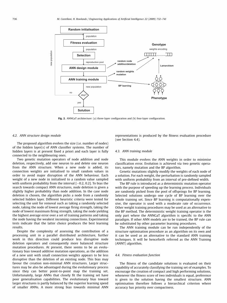
The EA architecture is shown in Fig. 2. The algorithmcomprises two components, namely, a structure design moduleand an ANN training module, that act concurrently on thesame pool of individuals. The system is designed with the purposeof obtaining maximum modularity between the two learningtasks.

The co-occurrence of the two modules is expected to bebeneficial for the effectiveness and the speed of the evolutionprocedure. That is, the presence of similarly performing structuralmutations of an individual is likely to favour population diversity.Moreover, the EA fitness function calculates the accuracy of asolution as the difference between the ANN output and thedesired output. Manipulation of the topology modifies the ANNoutput and hence the error surface, thus helping the weighttraining algorithm to escape local peaks or flat areas of fitness.Finally, parallel distributed processing systems such as ANNspossess well-known fault tolerance to addition or removal ofprocessing units. This capability minimises the number of fatalstructural mutations, since moderate changes of the ANNarchitecture are not likely to cause major disruption to theprogress of the learning procedure.

The genotype of each solution is characterised by a real-valuedvariable-length string that encodes the setting of the connectionweights. Each generation the fitness of the population is assessed,and then a cycle of the structure design module and a cycle of theANN training module are executed. Evolution is achieved viarandom genetic mutations affecting the ANN architecture and theweights. Fitness ranking (Fogel, 2000) is used to select the pool ofreproducing individuals. The BP rule is included into the ANNtraining module as a problem-specific operator. Experimentaltests carried out during the algorithm optimisation phase showedthat the use of the BP rule enhances the speed and the accuracy ofthe weight training procedure.

Because of the real-valued encoding of the solutions and thelack of genetic crossover the ANNGaT algorithm is conceptuallyakin to EP. This paradigm allows the candidate solutions to berepresented in a more compact format and avoids the manyproblems stemming from use of crossover.

As a result of the action of the two modules, a new populationis produced through genetic mutation and BP training of theexisting individuals. New solutions replace current ones viagenerational replacement (Fogel, 2000). The procedure is repeateduntil a pre-defined number of iterations has elapsed and thefittest solution of the last generation is picked.

ARTICLE IN PRESS

.......weights encoding

Genotype

Phenotype

random node addition/deletion

random weights mutation

Lamarckism

yes

Solution

population

population

reproduction pool

new population

no

new

pop

ulat

ion

Random initialisation

Fitness evaluation

Selection

ANN design module

ANN training module

stop?

BP learning

Fig. 2. ANNGaT architecture: (a) three-layer configuration and (b) four-layer configuration.

M. Castellani, H. Rowlands / Engineering Applications of Artificial Intelligence 22 (2009) 732–741736

4.2. ANN structure design module

The proposed algorithm evolves the size (i.e. number of nodes)of the hidden layer(s) of ANN classifier systems. The number ofhidden layers is at present fixed a priori and each layer is fullyconnected to the neighbouring ones.

Two genetic mutation operators of node addition and nodedeletion, respectively, add one neuron to and delete one neuronfrom the ANN structure. When a new node is added, itsconnection weights are initialised to small random values inorder to avoid major disruption of the ANN behaviour. Eachweight of a new node in initialised to a random value sampledwith uniform probability from the interval [�0.2, 0.2]. To bias thesearch towards compact ANN structures, node deletion is given aslightly higher probability than node addition. In the case nodedeletion is chosen, the algorithm picks a node from a randomlyselected hidden layer. Different heuristic criteria were tested forselecting the unit for removal such as taking a randomly selectednode, taking the node of lowest average firing strength, taking thenode of lowest maximum firing strength, taking the node yieldingthe highest average error over a set of training patterns and takingthe node having the weakest incoming connections. Experimentaltests indicate that the latter choice produces the best learningresults.

Despite the complexity of assessing the contribution of aprocessing unit in a parallel distributed architecture, furtherwork in this direction could produce less disruptive nodedeletion operators and consequently more balanced structuremutation procedures. At present, there seems to be an evolu-tionary bias toward additive mutation operations, as the additionof a new unit with small connection weights appears to be lessdisruptive than the deletion of an existing node. This bias mayfavour the creation non-minimal ANN structures. Larger struc-tures may be also be advantaged during the evolutionary processsince they can better point-to-point map the training set.Unfortunately, large ANNs that closely fit the training set havepoor generalisation capabilities. The evolutionary bias towardlarger structures is partly balanced by the superior learning speedof smaller ANNs. A more strong bias towards minimal ANN

representations is produced by the fitness evaluation procedure(see Section 4.4).

4.3. ANN training module

This module evolves the ANN weights in order to minimiseclassification error. Evolution is achieved via two genetic opera-tors, namely mutation and the BP algorithm.

Genetic mutations slightly modify the weights of each node ofa solution. For each weight, the perturbation is randomly sampledwith uniform probability from an interval of pre-defined width.

The BP rule is introduced as a deterministic mutation operatorwith the purpose of speeding up the learning process. Individualsare randomly picked from the pool of offsprings for BP learning.Selected solutions undergo one cycle of BP learning over thewhole training set. Since BP learning is computationally expen-sive, the operator is used with a moderate rate of occurrence.Other weight training procedures may be used as an alternative tothe BP method. The deterministic weight training operator is theonly part where the ANNGaT algorithm is specific to the ANNparadigm. If other ANN models are to be trained, the BP rule canbe substituted by other parameter learning procedures.

The ANN training module can be run independently of thestructure optimisation procedure as an algorithm on its own andit can be used as an alternative to the standard ANN trainingtechniques. It will be henceforth referred as the ANN Training(ANNT) algorithm.

4.4. Fitness evaluation function

The fitness of the candidate solutions is evaluated on theircapability of accurately classifying the training set of examples. Toencourage the creation of compact and high performing solutions,whenever the fitness score of two individuals is equal, preferenceis given to the solution having the smallest structure. ANNoptimisation therefore follows a hierarchical criterion whereaccuracy has priority over compactness.

ARTICLE IN PRESS

M. Castellani, H. Rowlands / Engineering Applications of Artificial Intelligence 22 (2009) 732–741 737

In general, there are cases where the difference in accuracybetween some of the solutions is very small (i.e., a few trainingexamples) in comparison to the spread of the population. In suchcases, it is more efficient to consider those solutions to be equallyperforming and give preference to the ones having the mosteconomical structure.

The proposed algorithm considers the accuracy of twoindividuals to be equal when the difference is less than onestandard deviation of the average population accuracy. That is, thepopulation is divided into a number of bins of width equal to

width ¼ max std_dva 1�gen

duration

� �;best �worst

popsize

� �(1)

where width is the width of the bin, std_dva is the standarddeviation of the fitness of the population, gen is the currentevolutionary cycle, duration is the duration of the learningprocedure, best and worst are the classification accuracies of,respectively, the best and the worst individual and popsize is thepopulation size.

The first bin is centred around the best performing solutionwhile the centres of the remaining bins are calculated accordingto the following formula:

centrei ¼ best � i width (2)

where centrei is the centre of the ith bin and i is an integer number(i ¼ 1,y, n) that is progressively increased until all the populationis grouped.

The proposed procedure aims at cutting part of the noise thataffects the evaluation of the candidate solutions. As the algorithmproceeds, the width of the bins is progressively shrunk to shift theemphasis on finer differences of accuracy. For each evaluation ofthe EA population, Eq. (1) limits the number of bins to a value thatis no greater than the population size.

Solutions are awarded the following pair of measures as fitnessscore:

fitnessj ¼ fn� i; sizejg (3)

where fitnessj is the fitness score of the jth member of thepopulation, i is the bin where the jth solution lies, n is the totalnumber of bins and sizej expresses the size of the MLP architectureas the total number of connection weights. Since the ANN is fullyconnected and the input and the output layers are fixed, sizej isdetermined by the size of the hidden layer(s).

The first fitness measure is proportionally related to theclassification accuracy. That is, the best performing solution(grouped into the first bin) has an accuracy score equal to n�1.All the solutions within half bin width from the accuracy of thebest individual obtain the same score. The solutions grouped intothe second bin obtain an accuracy score equal to n�2, and so forthuntil the last bin where solutions achieve an accuracy score equalto 0. Solutions having the same accuracy score (i.e., belonging tothe same bin) are further ranked according to the measure of theirsize by the fitness ranking procedure.

5. Experimental settings and results

This section presents the experimental settings and the resultsof the application of the ANNGaT algorithm to the generation ofthe MLP classifier for the wood veneer defect recognition taskdiscussed in Section 2.

5.1. Experimental set up

This section presents the results of five experiments. Namely,two tests concerning the BP training of manually optimised ANN

structures, one test concerning the training of a manuallyoptimised structure using the ANNT algorithm, and two testsconcerning the full ANNGaT algorithm. The result reported foreach of the experiments corresponds to the average of 20independent learning trials.

To simplify the training of the individuals, input data arenormalised according to the Mean–Variance procedure. A databalancing procedure is used. For each learning trial, the size of theclasses in the training set is made even by duplicating randomlypicked members of the smaller categories.

For each learning trial, the data set is randomly split into atraining set including 80% of the examples and a test set includingthe other 20%. The classifier is trained on the former and the finallearning result is evaluated on the latter. To reduce the danger ofoverfitting, the order of presentation of the training samples israndomly reshuffled for every learning cycle of the algorithmunder evaluation.

The first two experiments replicate the learning trials ofPackianather et al. (2000) and Pham and Sagiroglu (2000) andtrain the classifier using the BP rule with momentum term. Thefirst test is carried out using the ANN topology that Packianatheret al. (2000) optimised through the Taguchi method. Thisconfiguration is characterised by a hidden layer of 45 processingunits. Each neuron of the hidden layer receives 17+1 incomingconnections from the 17 input neurons and the bias neuron. Eachneuron of the output layer receives 45+1 incoming connectionsfrom the 45 hidden neurons and the bias neuron. The MLParchitecture is therefore composed of a total of 45�18+13�46 ¼1408 connection weights. The second test uses the ANN config-uration that Pham and Sagiroglu (2000) have experimentallydetermined. This configuration is characterised by two hiddenlayers of 17 processing units each. Likewise to the previous case,the total connectivity of the MLP architecture can be calculated toamount to 17�18+17�18+13�18 ¼ 846 connection weights. Theduration of the BP learning procedure is experimentally set to afixed number of iterations. The purpose of the first twoexperiments is to provide a baseline for the comparison of theresults.

The third experiment uses the ANNT algorithm to train amanually designed MLP classifier. The duration of the ANNTprocedure and the size of the ANN architecture is experimentallyset to maximise the learning accuracy. The best performingsolution consists of one hidden layer of 35 processing units. Theduration of the ANNT algorithm is experimentally fixed. Thepurpose of this test is to assess the performance of the ANNTprocedure, which is the evolutionary MLP training module of theANNGaT algorithm.

Finally, the last two experiments apply the full ANNGaTalgorithm to generate and train the wood veneer defect classifier.In the first test, the EA is used to design and train a three-layer(one hidden layer) MLP classifier. In the second test, the EA is usedto design and train a four-layer (two hidden layer) MLP classifier.In both the cases, the size of the hidden layer(s) of the startingpopulation is randomly initialised within the interval of integernumbers [15,25].

The optimisation of the learning algorithms is carried outaccording to experimental trial and error. Table 2 shows the mainMLP settings and the learning parameters used in the five tests.

5.2. Experimental results

The results of the five experiments are reported in Tables 3and 4. Table 3 details the design method used for the MLPclassifier, the mean and the standard deviation of the classifica-tion accuracy over the 20 learning trials, and the number of

ARTICLE IN PRESS

Table 2Parameter setting of Multi-Layer Perceptron and Learning Algorithms.

Multi-Layer Perceptron settings

Input nodes 17

Output nodes 13

Hidden layers a

MLP hidden nodes a

Activation function of hidden layer nodes Hyper-tangent

Activation function of output layer nodes Sigmoidal

Evolutionary Algorithm settings BP ANNT ANNGaT

Trials 20 20 20

learning cycles a a a

Population size – 100 100

MLP structure mutation rate (node addition) – – 0.0225

MLP structure mutation rate (node deletion) – – 0.0275

MLP weights mutation rate – 0.25 0.25

Amplitude MLP weights mut. – 0.2 0.2

BP Lamarckian operator rate – 0.6 0.6

BP Learning coefficient 0.01 0.01 0.01

BP Momentum term 0.1 – –

Initialisation range for MLP weights [�0.05, 0.05] [�0.05, 0.05] [�0.05, 0.05]

Initialisation range for MLP hidden nodes – – [15, 25]

a Depending from test.

Table 3Experimental results—classification accuracy.

BP ANNT ANNGaT

MLP design method Manual (P&S) Taguchi (P&O) Manual (authors) Evolutionary (three layers) Evolutionary (four layers)

Accuracy 78.09 82.02 82.34 80.00 80.64

Standard deviation 5.17 4.86 4.53 3.41 4.97

Upper bounda 80.50 84.29 84.46 81.60 82.97

Lower bounda 75.67 79.75 80.22 78.40 78.31

Learning cycles 4000 1500 2000 7000 2000

Manual (P&S), see Pham and Sagiroglu (2000).

Taguchi (P&O), see Packianather et al. (2000).a 95% confidence interval.

Table 4Experimental results—structure optimisation.

ANNGaT Manual (P&S) Taguchi (P&O) Manual (authors) ANNGaT—three layers ANNGaT—four layers

Average Max Min Average Max Min

Hidden layer 1 17 45 35 14.15 17 8 12.31 14 9

Hidden layer 2 17 – – – – – 12.25 16 9

Manual (P&S), see Pham and Sagiroglu (2000).

Taguchi (P&O), see Packianather et al. (2000).

M. Castellani, H. Rowlands / Engineering Applications of Artificial Intelligence 22 (2009) 732–741738

learning cycles. Table 3 reports also the upper and lower boundsof the 95% confidence interval for the accuracy results producedby the automatic and manual design methods. All accuracy resultsrefer to the percentage of successfully classified examples of thetest set. The number of learning cycles refers to the manuallyoptimised fixed duration of the algorithm. Table 4 shows theaverage, maximum and minimum size of the hidden layer(s)evolved by ANNGaT.

The first two experiments substantially confirm the resultsreported in the literature. That is, the average classificationaccuracy obtained by the three-layered MLP is within onestandard deviation from the 84.16% classification accuracyreported for the same architecture by Packianather et al. (2000).The average classification accuracy obtained by the four-layered

MLP is within two standard deviations from the 86.96%classification accuracy reported for the same architecture byPham and Sagiroglu (2000). The spread of the classificationaccuracy for the MLP configuration having 45 hidden neurons ishigher than the 1.52% estimate of Packianather et al. (2000).However, the latter estimate is calculated by running 9learning trials equally distributed on 3 randomly initialisedtraining and test set partitions, while the figure in Table 3 iscomputed from 20 learning trials, each of them on a differentrandomly initialised data set partition. The larger variabilityof the initial conditions may therefore explain the increasedspread of the data distribution. Overall, the two MLP configura-tions obtain comparable learning results in terms of accuracy androbustness.

ARTICLE IN PRESS

Three-Layer configuration - Classification Accuracy

0

10

20

30

40

50

60

70

80

90

100

Acc

urac

y

Population Average - Training SetBest Solution - Training SetBest Solution - Test Set

Four-Layer configuration - Classification Accuracy

0

10

20

30

40

50

60

70

80

90

100

0

Acc

urac

y

Generations

Population Average - Training SetBest Solution - Training SetBest Solution - Test Set

10000900080007000600050004000300020001000

0

Generations10000900080007000600050004000300020001000

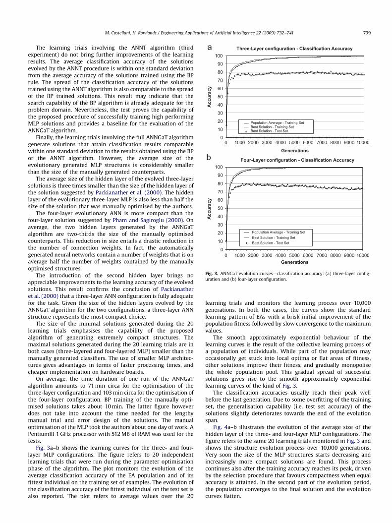
Fig. 3. ANNGaT evolution curves—classification accuracy: (a) three-layer config-

uration and (b) four-layer configuration.

M. Castellani, H. Rowlands / Engineering Applications of Artificial Intelligence 22 (2009) 732–741 739

The learning trials involving the ANNT algorithm (thirdexperiment) do not bring further improvements of the learningresults. The average classification accuracy of the solutionsevolved by the ANNT procedure is within one standard deviationfrom the average accuracy of the solutions trained using the BPrule. The spread of the classification accuracy of the solutionstrained using the ANNT algorithm is also comparable to the spreadof the BP trained solutions. This result may indicate that thesearch capability of the BP algorithm is already adequate for theproblem domain. Nevertheless, the test proves the capability ofthe proposed procedure of successfully training high performingMLP solutions and provides a baseline for the evaluation of theANNGaT algorithm.

Finally, the learning trials involving the full ANNGaT algorithmgenerate solutions that attain classification results comparablewithin one standard deviation to the results obtained using the BPor the ANNT algorithm. However, the average size of theevolutionary generated MLP structures is considerably smallerthan the size of the manually generated counterparts.

The average size of the hidden layer of the evolved three-layersolutions is three times smaller than the size of the hidden layer ofthe solution suggested by Packianather et al. (2000). The hiddenlayer of the evolutionary three-layer MLP is also less than half thesize of the solution that was manually optimised by the authors.

The four-layer evolutionary ANN is more compact than thefour-layer solution suggested by Pham and Sagiroglu (2000). Onaverage, the two hidden layers generated by the ANNGaTalgorithm are two-thirds the size of the manually optimisedcounterparts. This reduction in size entails a drastic reduction inthe number of connection weights. In fact, the automaticallygenerated neural networks contain a number of weights that is onaverage half the number of weights contained by the manuallyoptimised structures.

The introduction of the second hidden layer brings noappreciable improvements to the learning accuracy of the evolvedsolutions. This result confirms the conclusion of Packianatheret al. (2000) that a three-layer ANN configuration is fully adequatefor the task. Given the size of the hidden layers evolved by theANNGaT algorithm for the two configurations, a three-layer ANNstructure represents the most compact choice.

The size of the minimal solutions generated during the 20learning trials emphasises the capability of the proposedalgorithm of generating extremely compact structures. Themaximal solutions generated during the 20 learning trials are inboth cases (three-layered and four-layered MLP) smaller than themanually generated classifiers. The use of smaller MLP architec-tures gives advantages in terms of faster processing times, andcheaper implementation on hardware boards.

On average, the time duration of one run of the ANNGaTalgorithm amounts to 71 min circa for the optimisation of thethree-layer configuration and 103 min circa for the optimisation ofthe four-layer configuration. BP training of the manually opti-mised solutions takes about 10 min. The latter figure howeverdoes not take into account the time needed for the lengthymanual trial and error design of the solutions. The manualoptimisation of the MLP took the authors about one day of work. APentiumIII 1 GHz processor with 512 MB of RAM was used for thetests.

Fig. 3a–b shows the learning curves for the three- and four-layer MLP configurations. The figure refers to 20 independentlearning trials that were run during the parameter optimisationphase of the algorithm. The plot monitors the evolution of theaverage classification accuracy of the EA population and of itsfittest individual on the training set of examples. The evolution ofthe classification accuracy of the fittest individual on the test set isalso reported. The plot refers to average values over the 20

learning trials and monitors the learning process over 10,000generations. In both the cases, the curves show the standardlearning pattern of EAs with a brisk initial improvement of thepopulation fitness followed by slow convergence to the maximumvalues.

The smooth approximately exponential behaviour of thelearning curves is the result of the collective learning process ofa population of individuals. While part of the population mayoccasionally get stuck into local optima or flat areas of fitness,other solutions improve their fitness, and gradually monopolisethe whole population pool. This gradual spread of successfulsolutions gives rise to the smooth approximately exponentiallearning curves of the kind of Fig. 3.

The classification accuracies usually reach their peak wellbefore the last generation. Due to some overfitting of the trainingset, the generalisation capability (i.e. test set accuracy) of thesolutions slightly deteriorates towards the end of the evolutionspan.

Fig. 4a–b illustrates the evolution of the average size of thehidden layer of the three- and four-layer MLP configurations. Thefigure refers to the same 20 learning trials monitored in Fig. 3 andshows the structure evolution process over 10,000 generations.Very soon the size of the MLP structures starts decreasing andincreasingly more compact solutions are found. This processcontinues also after the training accuracy reaches its peak, drivenby the selection procedure that favours compactness when equalaccuracy is attained. In the second part of the evolution period,the population converges to the final solution and the evolutioncurves flatten.

ARTICLE IN PRESS

Three-Layer configuration - Structure Optimisation

02468

1012141618202224

Size

of L

ayer

Best Solution

0 10000900080007000600050004000300020001000

Four-Layer configuration - Structure Optimisation

02468

10121416182022

0

Size

of L

ayer

Generations

Best Solution - First Layer

Best Solution - Second Layer

10000900080007000600050004000300020001000

Generations

Fig. 4. ANNGaT evolution curves—ANN structure.

M. Castellani, H. Rowlands / Engineering Applications of Artificial Intelligence 22 (2009) 732–741740

6. Conclusions and further work

This study expands previous work on the classification of woodveneer defects from statistical features of wood sub-images usingan MLP classifier system. The generation of the MLP classifier isautomated following the introduction of ANNGaT, an evolutionaryprocedure for concurrent structure design and training of ANNsystems. The proposed algorithm evolves the size of the ANNhidden layer(s) while training the connection weights.

Experimental evidence shows the ANNGaT algorithm buildshighly compact MLP structures capable of accurate and robustlearning. The time duration of the proposed algorithm is veryreasonable.

Compared to the current approach based on the Taguchimethod for the manual optimisation of the MLP structure and onthe BP rule for the training of the connection weights, theproposed algorithm generates equally performing ANN solutionsusing considerably smaller architectures. On average, the size ofthe hidden layer of the three-layer MLP structures created by theANNGaT algorithm is three times smaller than the size of theempirically optimised three-layer configuration. Compared to analternative approach based on trial and error optimisation of theANN structure, the ANNGaT algorithm generates four-layer ANNstructures that are on average two-thirds the size of the manuallygenerated counterparts. In both the cases, the proposed algorithmclearly requires lower design costs since the process is fullyautomated.

Further investigation on the impact of the structure modifica-tion operations on the ANN behaviour could help to produce lessdisruptive mutation procedures. Improvement of the proposedalgorithm may also result from submitting the EA learning

parameters, namely the weight mutation stepsize and the BPlearning rate to the evolutionary process. Finally, since differentANN architectures and learning parameters are characterised bydifferent learning curves, niching techniques could be used to letdifferently parameterised sub-populations evolve separately be-fore submitting them to competition. Such approach would allowmore informed evaluations of the candidate solutions.

References

Aboitiz, F., 1992. Mechanisms of adaptive evolution—Darwinism and Lamarckismrestated. Medical Hypotheses 38 (3), 194–202.

Angeline, P.J.a., Fogel, D.B., 1997. An evolutionary program for the identification ofdynamical systems. In: Rogers, S. (Ed.), Proceedings of SPIE Volume 3077:Application and Science of Artificial Neural Networks III. SPIE The InternationalSociety for Optical Engineering, Bellingham, WA, pp. 409–417.

Angeline, P.J., Sauders, G.M., Pollack, J.B., 1994. An evolutionary algorithm thatconstructs recurrent neural networks. IEEE Transactions Neural Networks 5(1), 54–65.

Balakrishnan, K., Honavar, V., 1995. Evolutionary design of neural architectures—

a preliminary taxonomy and guide to literature. Technical Report CS TR95-01,Department of Computer Science, Iowa State University, Ames.

Branke, J., 1995. Evolutionary algorithms for neural network design and training.Technical Report No. 322, Institute AIFB, University Karlsruhe.

Brown, A.D., Card, H.C., 1999. Cooperative-competitive algorithms for evolutionarynetworks classifying noisy digital images. Neural Processing Letters 10 (3),223–229.

Cangelosi, A., Elman, J.L., 1995. Gene regulation and biological development inneural networks: an exploratory model. Technical Report, CRL-UCSD, Uni-versity of California San Diego.

Castillo, P.A., Carpio, J., Merelo, J.J., Prieto, A., Rivas, V., Romero, G., 2000. Evolvingmultilayer perceptrons. Neural Processing Letters 12 (2).

Darwen, P.J., 2000. Black magic: interdependence prevents principled parametersetting, self-adapting costs too much computation. In: Applied Complexity:From Neural Nets to Managed Landscapes, pp. 227–237.

Eiben, A.E., Smith, J.E., 2003. Introduction to Evolutionary Computing. Springer,New York.

Fahlman, S.E., Lebiere, C., 1990. The cascade-correlation learning architecture. In:Touretzky, D.S. (Ed.), Advances in Neural Information Processing Systems 2.Morgan Kaufmann, San Mateo, CA, pp. 524–532.

Fogel, D.B., 2000. Evolutionary Computation: Toward a New Philosophy of MachineIntelligence, second ed. IEEE Press, New York.

Fogel, D.B., Chellapilla, K., 2002. Verifying Anaconda’s expert rating by competingagainst Chinook: experiments in co-evolving a neural checkers player.Neurocomputing (42), 69–86.

Fogel, D.B., Fogel, L.J., Porto, V.W., 1990. Evolutionary programming for trainingneural networks. In: Proceedings International Joint Conference on NNs, SanDiego, CA, June 1990, pp. 601–605.

Fogel, L.J., Owens, A.J., Walsh, M.J., 1966. Artificial Intelligence Through SimulatedEvolution. Wiley, New York.

Gomez, F.J., Miikkulainen, R., 2003. Active guidance for a finless rocket throughneuroevolution. In: Proceedings of the 2003 Genetic and EvolutionaryComputation Conference (GECCO), Chicago IL, pp. 2084–2095.

Hancock, P.J.B., 1992. Genetic algorithms and permutation problems: a comparisonof recombination operators for neural structure specification. In: Whitely, D.,Schaffer, J.D. (Eds.), Combinations of Genetic Algorithms and Neural Networks.IEEE Computer Society Press.

Harp, S.A., Samad, T., Guha, A., 1990. Designing application-specific neuralnetworks using the genetic algorithm. In: Touretzky, D.S. (Ed.), Advances inNeural Information Processing Systems 2. Morgan Kaufmann, San Mateo, CA,pp. 447–454.

Haussler, A., Li, Y., Ng, K.C., Murray-Smith, D.J., Sharman, K.C., 1995. Neurocon-trollers designed by a genetic algorithm. In: Proceedings of the GALESIA FirstIEE/IEEE International Conference on GAs in Engineering Systems: Innovationsand Applications, Sheffield UK, 1995, pp. 536–542.

Holland, J.H., 1975. Adaptation in Natural and Artificial Systems. University ofMichigan Press, Ann Arbor, MI.

Huber, H.A., McMillin, C.W., McKinney, J.P., 1985. Lumber defect detection abilitiesof furniture rough mill employees. Forest Products Journal 35 (11/12), 79–82.

Husken, M., Igel, C., 2002. Balancing learning and evolution. In: Proceedings of theGeneric and Evolutionary Computation Conference, (GECCO-2002), SanFrancisco, CA, USA, pp. 391–398.

Johansson, E.M., Dowla, F.U., Goodman, D.M., 1991. Backpropagation learning formultilayer feed-forward neural networks using the conjugate gradientmethod. International Journal Neural Systems 2 (4), 291–301.

Jung, S.Y., 2005. A topographical method for the development of neural networksfor artificial brain evolution. Artificial Life (11), 293–316.

Kitano, H., 1990. Designing neural networks using genetic algorithms with graphgeneration system. Complex Systems 4 (4), 461–476.

Lappalainen, T., Alcock, R.J., Wani, M.A., 1994. Plywood feature definition andextraction. Report 3.1.2, QUAINT, BRITE/EURAM Project 5560, IntelligentSystems Laboratory, School of Engineering, University of Wales, Cardiff.

ARTICLE IN PRESS

M. Castellani, H. Rowlands / Engineering Applications of Artificial Intelligence 22 (2009) 732–741 741

LeCun, Y., Denker, J.S., Solla, S.A., 1990. Optimal brain damage. In: Touretzky, D.S.(Ed.), Advances in Neural Information Processing Systems 2. MorganKaufmann, San Mateo, CA, pp. 598–605.

Menczer, F., Parisi, D., 1992. Evidence of hyperplanes in the genetic learning ofneural networks. Biological Cybernetics 66, 283–289.

Miller, G.F., Todd, P.M., Hegde, S.U., 1989. Designing neural networks using geneticalgorithms. In: Proceedings of the Third International Conference on GAs andApplications, Arligton, VA, 1989, pp. 379–384.

Montana, D., Davis, L., 1989. Training feedforward neural networks using geneticalgorithms. In: Proceedings of the 11th International Joint Conference on AI,Detroit, MI, 1989, pp. 762–767.

Nikolaev, N.Y., 2003. Learning polynomial feedforward neural networks by geneticprogramming and backpropagation. IEEE Transactions on Neural Networks 14(2), 337–350.

Packianather, M., 1997. Design and optimisation of neural network classifiers forautomatic visual inspection of wood veneer. Ph.D. Thesis, University of Wales,College of Cardiff (UWCC), UK.

Packianather, M.S., Drake, P.R., Rowlands, H., 2000. Optimising the parameters ofmultilayered feedforward neural networks through Taguchi design of experi-ments. Quality and Reliability Engineering International 16, 461–473.

Parekh, R., Yang, J.H., Honavar, V., 2000. Constructive neural-network learningalgorithms for pattern classification. IEEE Transactions on Neural Networks 11(2), 436–451.

Pham, D.T., Alcock, R.J., 1996. Automatic detection of defects on birch wood boards.Proceedings of Institution of Mechanical Engineers, Part E, Journal of ProcessMechanical Engineering 210, 45–52.

Pham, D.T., Alcock, R.J., 1999a. Recent developments in automated visualinspection of wood boards. In: Tzafestas (Ed.), Advances in Manufacturing:Decision, Control and Information Technology. Springer, London, pp. 80–88.

Pham, D.T., Alcock, R.J., 1999b. Plywood image segmentation using hardware-basedimage processing functions. Proceedings of Institution of MechanicalEngineers, Part B 213, 431–434.

Pham, D.T., Alcock, R.J., 1999c. Automated visual inspection of wood boards:selection of features for defect classification by a neural network. Proceedingsof Institution of Mechanical Engineers, Part E 213, 231–245.

Pham, D.T., Liu, X., 1995. Neural Networks for Identification, Prediction and Control.Springler, London.

Pham, D.T., Sagiroglu, S., 2000. Neural network classification of defects in veneerboards. Proceedings of Institution of Mechanical Engineers, Part B 214,255–258.

Polzleitner, W., Schwingshakl, G., 1992. Real-time surface grading of profiledwooden boards. Industrial Metrology 2, 283–298.

Rechenberg, I., 1965. Cybernetic Solution Path of an Experimental Problem, LibraryTranslation No. 1122. Ministry of Aviation, Royal Aircraft Establishment,Farnborough, Hants, UK.

Reed, R., 1993. Pruning algorithms—a survey. IEEE Transactions Neural Networks 4,740–747.

Roy, R.K., 2001. Design of Experiments Using The Taguchi Approach: 16 Steps toProduct and Process Improvement. Wiley, New York.

Rumelhart, D.E., McClelland, J.L., 1986. Parallel Distributed Processing: Explorationin the Micro-Structure of Cognition, vol. 1–2. MIT Press, Cambridge.

Rychetsky, M., Ortmann, S., Glesner, M., 1998. Correlation and regression basedneuron pruning strategies. In: Fuzzy-Neuro-Systems ‘98, Fifth InternationalWorkshop, Munich D, Germany.

Saravanan, N., Fogel, D.B., 1994. Evolving neurocontrollers using evolutionaryprogramming. In: Proceedings of the First IEEE Conference on EvolutionaryComputation (ICEC), Orlando, FL, 1994, pp. 217–222.

Schiffmann, W., 2000. Encoding feedforward networks for topology optimizationby simulated evolution. In: Proceedings of the Fourth International Conferenceon Knowledge-Based Intelligent Engineering Systems & Allied Technologies(KES ‘2000), vol. 1, pp. 361–364.

Seiffert, U., 2001. Multiple layer perceptron training using genetic algorithms. In:Proceedings of the Ninth European Symposium on Artificial Neural Networks(ESANN 2001), Bruges B, pp. 159–164.

Skinner, A., Broughton, J.Q., 1995. Neural networks in computational materialsscience: training algorithms. Modelling and Simulation in Materials Scienceand Engineering 3, 371–390.

Smieja, F.J., 1993. Neural network constructive algorithms: trading generalizationfor learning efficiency? Circuits, Systems and Signal Processing 12 (2),331–374.

Srinivas, M., Patnaik, L.M., 1991. Learning neural network weights using geneticalgorithms—improving performance by search-space reduction. In: Proceed-ings of the 1991 IEEE International Joint Conference on Neural NetworksIJCNN’91, Singapore, vol. 3. IEEE Press, New York, NY, pp. 2331–2336.

Stepniewski, S.W., Keane, A.J., 1996. Topology design of feedforward neuralnetworks by genetic algorithms. In: Proceedings of the Fourth Inter-national Conference on Parallel Problem Solving from Nature (PPSN IV), pp.771–780.

Thierens, D., Suykens, J., Vanderwalle, J., De Moor, B., 1993. Genetic weightoptimisation of a feedforward neural network controller. In: Albrecht, R.F.,Reeves, C.R., Steele, N.C. (Eds.), Artificial Neural Networks and GeneticAlgorithms. Springler, Wien, pp. 658–663.

Whitley, D., 1995. Genetic algorithms and neural networks. In: Winter, G., Periaux,J., Galan, M., Cuesta, P. (Eds.), Genetic Algorithms in Engineering and ComputerScience. Wiley, pp. 203–216.

Whitley, D., Hanson, T., 1989. Optimising neural networks using faster, moreaccurate genetic search. In: Proceedings of the Third International Conferenceon GAs and Applications, Arligton, VA, 1989, pp. 391–396.

Yao, X., 1999. Evolving artificial neural networks. Proceedings of the IEEE 87 (9),1423–1447.

Yao, X., Liu, Y., 1997a. Fast evolution strategies. In: Proceedings of the Sixth AnnualConference on Evolutionary Programming (EP97), Lecture Notes in ComputerScience, vol. 1213. Springer, Berlin, pp. 151–161.

Yao, X., Liu, Y., 1997b. A new evolutionary system for evolving artificial neuralnetworks. IEEE Transactions on Neural Networks 8 (3), 694–713.

Yan, W., Zhu, Z., Hu, R., 1997. Hybrid genetic/BP algorithm and its application forradar target classification. In: Proceedings of the 1997 IEEE National Aerospaceand Electronics Conference, NAECON Part 2, pp. 981–984.

Doctor Marco Castellani obtained his Ph.D. degree in 2000 from University ofWales, Cardiff with a thesis on intelligent control of manufacturing of fibre opticcomponents. Between 2001 and 2002, he worked for a private company inGermany on machine learning applications to natural language processing.Between 2002 and 2005, he was at the New University of Lisbon, where hisresearch work included machine learning, machine vision, remote sensing, patternrecognition and time series prediction.

Professor Hefin Rowlands is Director of Research & Enterprise at the University ofWales, Newport with responsibilities for developing the research culture andenvironment for staff and postgraduate students across the University. Hisdoctorate thesis was on optimum design using Taguchi method with neuralnetworks and genetic algorithms. He was awarded a University of Wales PersonalChair in 2002 and his current research interests are concerned with investigatingthe benefits companies achieve from deploying business improvement techniquessuch as six sigma.