Evolution of preference orderings for the Deterrence …ecl/papers/1709.cs-tr-17-04.pdfEvolution of...

Evolution of preference orderings for the Deterrence Game

Annie S. Wu1, Ramya Pradhan1, Lisa J. Carlson2, Raymond Dacey3, Robert B. Heckendorn4

September 13, 2017

Technical report number: CS-TR-17-04

1Department of Computer Science, University of Central Florida, Orlando, FL 32816-23622Department of Political Science, University of Idaho, Moscow, ID 838443Department of Business, University of Idaho, Moscow, ID 838444Department of Computer Science, University of Idaho, Moscow, ID 83844

Abstract

We investigate the evolution and survival of decision making strategies for the Deterrence Gamein a population of interacting agents. The Deterrence Game is a sequential, two player game that isused to study how player preference orderings affect the outcome in situations of conflict. Althoughthere are twenty-four possible player preference orderings, only five are given serious theoretical at-tention in the deterrence literature. We use analytical and empirical approaches to investigate whatare the characteristics that make a preference ordering competitive or uncompetitive and whetherthe five traditionally studied preference orderings are the most competitive for their roles. Resultsfind that four out of the five traditionally studied preference orderings are highly competitive. Thefifth preference ordering is analytically moderately competitive but empirically unsuccessful. Anal-ysis of all twenty-four preference orderings indicates that there are additional preference orderingsthat behave identically to the traditional five and are competitive.

1 Introduction

In this paper, we investigate the evolution and survival of decision making strategies in situations ofconflict using the Traditional Deterrence Game. The Traditional Deterrence Game (Zagare and Kilgour1993; Morrow 1994) is a sequential, two player game that is used to study situations of conflict. Thegame consists of two players or agents and each player has one or two decision points at which it mustchoose between one of two actions. The players’ interaction produces one of four possible outcomes.Agents are distinguished by their preference ordering over the four outcomes. Four possible outcomesgives a total of 4! = 24 possible preference orderings over the outcomes. Interestingly, only five ofthe twenty-four possible preference orderings are given serious theoretical attention in the deterrenceliterature (Zagare and Kilgour 1993; Morrow 1994; Simon 2002; Zagare and Kilgour 2000). We examinewhether these five preference orderings are the optimal strategies for agents to apply in each role of aDeterrence Game; whether there are other competitive preference orderings, aside from the traditionalfive, that perform well in a Deterrence Game; and what characteristics make a preference orderingcompetitive or uncompetitive.

1

We begin by examining the outcomes of all possible instances of a Deterrence Game and find that,although there are twenty-four possible preference orderings for each player, many preference orderingsexhibit identical behavior. Grouping the preference orderings with like behavior into classes producesseven classes of Challengers and four classes of Defenders. For each class, we can determine the featuresthat are common among all preference orderings in that class. We define a measure of survivability anduse it to calculate the expected survivability of each class of preference orderings. We then comparethe estimated survivability with results from an agent-based simulation of a population of interactingagents playing the Deterrence Game.

Our analysis finds that the five traditionally studied preference orderings are among those withthe highest expected survivability. While two of these preference orderings are the only member oftheir class, the other three preference orderings belong to classes which include additional preferenceorderings that exhibit identical behavior. Results from the agent-based simulation indicate that fourof the five traditional preference orderings are competitive when played against all possible preferenceorderings. Not surprisingly, the preference orderings that survive in a simulation depend in part on whatpreference orderings are included in the player pool. The fact that most of the preference orderingsstudied within the context of the Traditional Deterrence Game are competitive and survive in thesimulation is a particularly interesting result. The simulation shows that these preference orderings canbe considered endogenous to formal models of deterrence and provides justification for why they shouldbe studied. The simulation also suggests that there may be other competitive preference orderings thatmerit theoretical attention.

2 Background and motivation

Deterrence refers to “...the use of threats by one party to convince another party to refrain from initiatingsome course of action” (Huth 1999). Deterrence is a ubiquitous phenomenon. Parents try to preventtheir children from engaging in unwanted behavior. Legislators pass laws to discourage citizens frombehaving in certain ways. Nation-states try to prevent other states from attacking them. The alphamale of a species attempts to discourage potential interlopers. These examples show that deterrence isa central component of many human and non-human interactions. Understanding deterrence is therebyimportant, and relevant to, many fields of inquiry including biology (da Cruz, Gaspar, and Calado 2012;Ruxton, Sherratt, and Speed 2004), business and economics (Barbot, Betancor, Socorro, and Viecens2014; Ossa 2014), psychology (Mooijman, van Dijk, Ellemers, and van Dijk 2015; Pantaleo, Miron,Ferguson, and Frankowski 2014; Scheber 2011), law and sociology (Durlauf, Fu, and Navarro 2013;Kagan 2016), international relations (Johnson, Leeds, and Wu 2015; Modongal 2016; Payne 2015), andcomputational science (Misra 2014; Wang and Wang 2016) Consequently, we can gain deeper insightinto the problem of deterrence by employing a multidisciplinary approach such as the one pursued here.

The Deterrence Game is a sequential game that is used to study interactions in which one agent,called Defender, may or may not be able to deter the challenge mounted by another agent, calledChallenger. It is typically used to model situations in which a new upstart considers mounting achallenge against an established veteran to change the status quo (Ellsberg 1961; Huth 1999; Jervis1979; Morgan 1977; Russett 1963; Schelling 1966). The effectiveness of a deterrence strategy depends onmultiple factors, including but not limited to, the credibility of the players’ threats to retaliate (Bramsand Kilgour 1985; Huth 1999; Nalebuff 1991; Powell 1990; Zagare 1987; Zagare and Kilgour 1993) andthe players’ valuation of the status quo (Carlson and Dacey 2006). These factors are reflected in partin the players’ preference orderings for the four possible outcomes of the game.

Figure 1 shows the decision tree of the Deterrence Game. Nodes indicate decision points and leavesindicate outcomes. There are two decision points for Challenger, C1 and C2, and one decision point

2

Persist

Comply AcquiesceC1

C2

D1Challenge

Resist

Accept

Desist

Status Quo

Capitulate

War

Figure 1: Decision tree for the traditional Deterrence Game.

Name Preference Ordering Name Preference Ordering@ WAR > CAP > ACQ > SQ l WAR > SQ > CAP > ACQa CAP > WAR > ACQ > SQ m CAP > SQ > WAR > ACQb WAR > ACQ > CAP > SQ n WAR > SQ > ACQ > CAPc CAP > ACQ > WAR > SQ o CAP > SQ > ACQ > WARd ACQ > WAR > CAP > SQ p ACQ > SQ > WAR > CAPe ACQ > CAP > WAR > SQ q ACQ > SQ > CAP > WARf WAR > CAP > SQ > ACQ r SQ > WAR > CAP > ACQg CAP > WAR > SQ > ACQ s SQ > CAP > WAR > ACQh WAR > ACQ > SQ > CAP t SQ > WAR > ACQ > CAPi CAP > ACQ > SQ > WAR u SQ > CAP > ACQ > WARj ACQ > WAR > SQ > CAP v SQ > ACQ > WAR > CAPk ACQ > CAP > SQ > WAR w SQ > ACQ > CAP > WAR

Table 1: The twenty-four possible preference orderings of the Deterrence Game. The column labeledName indicates the name assigned to each preference ordering. These names will be used to refer totheir corresponding preference orderings in the remainder of this paper. The use of the @ characterinstead of the a character as the name of the first preference ordering allows our results to be compareddirectly with that of Carlson et al. (2008).

for Defender, D1. The game begins at C1 when Challenger makes a decision about whether or not tomount a challenge against Defender. If Challenger decides not to mount a challenge, the game endswith an outcome of Status Quo (S). If Challenger decides to mount a challenge, the game moves tothe D1 node, and the decision making onus shifts to Defender. At D1, if Defender decides to defer toChallenger, the game ends with an outcome of Acquiesce (A). If Defender decides to resist Challenger’schallenge, the game moves to node C2 and the decision making onus reverts back to Challenger. AtC2, if Challenger decides to give in to Defender, the game ends with an outcome of Capitulate (C). IfChallenger decides to persist with its challenge, then the game moves to an outcome of War (W).

The decisions that Challenger and Defender make at their respective nodes are dictated by theagents’ preference ordering for the four possible outcomes. Table 1 lists the twenty-four preferenceorderings that are possible given four outcomes. In this work, we assume that the game is played underperfect and complete information. As a result, Challenger using preference ordering p (A > S > W >C) playing Defender using preference ordering m (C > S > W > A) will result in an outcome of S.This outcome of S is determined by a process known as backward induction. At node C2, Challenger’s

3

Name Code Letter Preference OrderingResolute Defender m CAP > SQ > WAR > ACQIrresolute Defender o CAP > SQ > ACQ > WARResolute Challenger p ACQ > SQ > WAR > CAPIrresolute Challenger q ACQ > SQ > CAP > WARRogue Challenger j ACQ > WAR > SQ > CAP

Table 2: The five commonly studied Deterrence Game preference orderings.

decision is based on whether Challenger prefers W to C or C to W. Since Challenger prefers W overC, Challenger chooses Persist which would give an outcome of W. At node D1, since Defender prefersW to A, Defender chooses Resist. At node C1, Challenger knows that, if Defender chooses Resist, thatChallenger will choose Persist at its final decision resulting in an outcome of W. Because Challengerprefers S to W, Challenger chooses not to challenge at node C1, resulting in a final game outcome of S.

Recall that we are interested in examining the evolution and survival of the various decision makingstrategies in the Deterrence Game in a population of interacting agents. The Deterrence Game presentedabove is simple, yet very useful and well suited, to explore the research question of immediate relevancein this paper. The model uncovers the basic structure of any deterrence situation, and thereby, allows usto examine the survivability of a particular preference ordering against all other possible combinationsof preference orderings. As such, it is unnecessary to construct a more sophisticated Deterrence Gamesince the increase in modeling complexity would not add any appreciable explanatory power given ourinterest here. For those interested in more complex deterrence models employed to address differentresearch questions, see (Langlois and Langlois 2005; Powell 1990; Zagare and Kilgour 2000).

The majority of the deterrence literature focuses on only five of the twenty-four possible preferenceorderings (Zagare and Kilgour 1993; Morrow 1994; Simon 2002; Zagare and Kilgour 2000). Thesefive preference orderings are Resolute Defender (m), Irresolute Defender (o), Resolute Challenger (p),Irresolute Challenger (q), and Rogue Challenger (j)1. Table 2 gives the names and preferences orderingsof these five players. Carlson et al. (2008) present one of the first studies that include all twenty-fourpossible deterrence preference orderings. Using an agent-based simulation, Carlson et al. (2008) examinethe evolution of a population of preference orderings over time. The population consists of agents eachof which is assigned a preference ordering. Agents are selected, two at a time, to play each otherin the Deterrence Game. The winner of a game is the agent whose preference ordering has a higherpreference for the resulting outcome. For example, Challenger using preference ordering p (A > S > W> C) playing Defender using preference ordering o (C > S > A > W) will result in an outcome of A.Because A is p’s highest preference and o’s third-highest preference, the winner is p. When there is awinner in a game, the winning agent replaces the losing agent in the population. If both agents haveequal preference for the resulting outcome, the game is tied and both players remain in the population.Table 3 shows the five stable or semi-stable sets of preference orderings that emerge. Each level consistsof the set of preference orderings that survive when all preference orderings in the previous levels areremoved from the population. Thus, level 1 preference orderings (r, s, t, u, v, w) are the ones thatsurvive when all twenty-four preference orderings compete, level 2 preference orderings (l, m, p, q) arethose that survive when all preference orderings minus the level 1 preference orderings compete, andso on. The first and most stable set is the set of all preference orderings that prefer S over all otheroutcomes. It is natural for these preference orderings thrive in this model because Challenger makesthe first move, and a Challenger that prefers S achieves the highest payoff and is always the winner.The explanation for the remaining sets is less clear and it is unclear how these sets relate to the five

1The terms “Hard” and “Soft” have also been used in place of “Resolute” and “Irresolute”, respectively, in theliterature.

4

Level Preference Orderings1 r, s, t, u, v, w2 l, m, p, q3 b, c, h, i, n, o4 @, a, f , g5 d, e, j, k

Table 3: The five emergent sets of preference orderings from (Carlson et al. 2008). Each level consistsof the preference orderings that survive when all preference orderings in the previous levels have beenremoved from the population.

traditionally studied preference orderings.

The work in this paper extends that of Carlson et al. (2008) by addressing two potential weaknessesthat we believe may have lead to the inconclusive results.

1. Carlson et al. (2008) use an agent’s preference for an outcome to determine the winner of a game.As a result, when Challenger with preference ordering a (C > W > A > S) plays Defender withpreference ordering f (W > C > S > A) and produces an outcome of C, the winner of the gameis Challenger despite the fact that the meaning of the outcome is that Challenger capitulates toDefender. Challenger replaces Defender because the outcome C is Challenger’s most preferredoutcome while the outcome C is Defender’s second most preferred outcome.

We will use the logical intent of an outcome to determine the winner of a game. As a result,if the outcome is that Challenger capitulates (C) to Defender, then Defender wins and replacesChallenger. If the outcome is that Defender acquiesces (A) to Challenger’s challenge, then Chal-lenger wins and replaces Defender. If the outcome is status quo (S), no one wins and both playersremain unchanged. An appropriate action for the outcome of war (W) is less straightforward. Inthis work, we characterize war as unpredictable and disruptive and consider two possible actionsthat reflect this characterization: (1) random-winner, where a winner is chosen randomly fromamong the two players to replace the loser or (2) random-replace, where both players are replacedby new, randomly generated players (i.e. both Challenger and Defender preference orderings arereplaced by one of the twenty-four possible preference orderings, randomly selected).

2. Carlson et al. (2008) assign a single preference ordering to each agent in their population. Thispreference ordering is used regardless of what role (Challenger or Defender) the agent is playingin a given game. Thus, that study is actually evolving for preference orderings that are successfulin both roles at the same time. A strong Challenger preference ordering, however, may or maynot be able to also be a strong Defender preference ordering.

We assign two preference orderings to each agent in our population, a challenger preference order-ing and a defender preference ordering. Depending on what role an agent is chosen to play, thecorresponding preference ordering will be used. As a result, the selection pressure on any givenpreference ordering will be focused towards a single role producing, we expect, stronger preferenceorderings for each role and more conclusive results.

3 Analysis of outcome table

Twenty-four possible Challenger preference orderings and twenty-four possible Defender preference or-derings gives 576 possible instances of the Deterrence Game. Table 4 lists the outcomes for all 576

5

Defender Strategy Challenger Class

@ a b c d e f g h i j k l m n o p q r s t u v w C0 C1 C2 C3 C4 C5 C6

Challenger @ W W W A A A W W W A A A W W W A A A W W W A A A X

Strategy a C C A C A A C C A C A A C C A C A A C C A C A A X

b W W W A A A W W W A A A W W W A A A W W W A A A X

c C C A C A A C C A C A A C C A C A A C C A C A A X

d W W W A A A W W W A A A W W W A A A W W W A A A X

e C C A C A A C C A C A A C C A C A A C C A C A A X

f W W W S S S W W W S S S W W W S S S W W W S S S X

g C C S C S S C C S C S S C C S C S S C C S C S S X

h W W W A A A W W W A A A W W W A A A W W W A A A X

i C C A C A A C C A C A A C C A C A A C C A C A A X

j W W W A A A W W W A A A W W W A A A W W W A A A X

k C C A C A A C C A C A A C C A C A A C C A C A A X

l W W W S S S W W W S S S W W W S S S W W W S S S X

m C C S C S S C C S C S S C C S C S S C C S C S S X

n W W W S S S W W W S S S W W W S S S W W W S S S X

o C C S C S S C C S C S S C C S C S S C C S C S S X

p S S S A A A S S S A A A S S S A A A S S S A A A X

q S S A S A A S S A S A A S S A S A A S S A S A A X

r S S S S S S S S S S S S S S S S S S S S S S S S X

s S S S S S S S S S S S S S S S S S S S S S S S S X

t S S S S S S S S S S S S S S S S S S S S S S S S X

u S S S S S S S S S S S S S S S S S S S S S S S S X

v S S S S S S S S S S S S S S S S S S S S S S S S X

w S S S S S S S S S S S S S S S S S S S S S S S S X

Defender D0 X X X X X X X X

Class D1 X X X X

D2 X X X X

D3 X X X X X X X X

Table 4: The Deterrence Game outcome table. This table lists all possible Deterrence Game outcomes.The Challenger and Defender classes indicate groups of preference orderings that behave identically.

possible pairings. Of particular interest are the following: row p gives the outcomes of Resolute Chal-lenger against every possible Defender, row q gives the outcomes of Irresolute Challenger against everypossible Defender, row j gives the outcomes of Rogue Challenger against every possible Defender, col-umn m gives the outcomes of Resolute Defender against every possible Challenger, and column o givesthe outcomes of Irresolute Defender against every possible Challenger.

Examination of the outcome table finds that many of the rows and columns are identical, indicatingthat those players are basically using the same decision making strategy. Grouping these identicalplayers into classes gives a total of seven challenger classes (C0-C6) and four defender classes (D0-D3).

To better understand which of these classes are competitive and which are not in a populationwide simulation, we identify the unique traits of each class of preference orderings and analyze theirimpact on game performance. We begin by defining a measure of survivability that calculates, for agiven preference ordering, the probability that it will win when played against all possible opponents.We then examine the members of each class to identify defining characteristics. We expect that theresults of these analyses will allow us to make predictions as to which classes of preference orderingsare most competitive.

3.1 Estimating survival probability

The survival probability of a preference ordering is the probability that a player using that preferenceordering will survive (not be replaced) when playing any possible opponent. To estimate the survivalprobability of a given preference ordering, we first define the probability that a player using thatpreference ordering will survive a single instance of the Deterrence Game then aggregate its likelihoodof survival against all possible opponents.

6

Outcome, φ Action PC(φ) PD(φ)S No action 1.0 1.0

(Status quo)A Challenger replaces Defender 1.0 0.0

(Defenderacquiesces)

C Defender replaces Challenger 0.0 1.0(Challengercapitulates)

W random-winner: Randomly select 0.5 0.5(War) a winner to replace the loser

random-replace: Randomly 0.042 0.042replace both players

Table 5: Actions and survival probability for each outcome, φ, of the Deterrence Game. PC(φ) andPD(φ) indicate the probability that Challenger and Defender, respectively, will survive outcome φ. Forthe W outcome, we consider two possible actions, random-winner and random-replace.

3.1.1 Surviving a single instance of the Deterrence Game

The probability that each player, Challenger and Defender, will survive a single instance of the Deter-rence Game is determined by the action that our simulation takes for each outcome, φ. In both the(Carlson, Dacey, Heckendorn, and Wu 2008) simulation and our simulation, a population of interactingagents evolves over time as pairs of agents are selected to play the Deterrence Game and agents that“win” replace agents that “lose”. Recall that we use the logical intent of an outcome to determine the“winner” of a game. Table 5 gives the actions that take place for each outcome in our simulation andthe resulting survival probabilities for both Challenger and Defender.

We can define, for our simulation, the probability that Challenger will survive a game, PC(φ),and the probability that Defender will survive a game, PD(φ), based on the actions in Table 5. Whenthe outcome of a game is φ = S, no action occurs and both players are unchanged. As a result, bothChallenger and Defender have a 100% probability of surviving the game and PC(S) = PD(S) = 1.0.When the outcome of a game is φ = A, Challenger wins and replaces Defender; thus, PC(A) = 1.0 andPD(A) = 0.0. When the outcome of a game is φ = C, Defender wins and replaces Challenger; thus,PC(C) = 0.0 and PD(C) = 1.0. When the outcome of a game is φ = W, we define probabilities forboth random-winner and random-replace. Under the random-winner action, one of the two players israndomly selected as the winner. As a result, both Challenger and Defender have a 50% probabilityof surviving the game and PC(W ) = PD(W ) = 0.5. Under the random-replace action, both playersare replaced by a randomly generated player. Because each preference ordering can be replaced by oneof twenty-four possible preference orderings, the probability that the preference ordering used in thecurrent game will survive is PC(W ) = PD(W ) = 1/24 = 0.042.

3.1.2 Aggregating over all possible opponents

Given the probabilities from Table 5 and the outcomes from Table 4, we can then estimate, for anypreference ordering and role, the likelihood that a player will survive any instance of the DeterrenceGame by aggregating the probabilities of that player surviving a game against every possible opponent.

The probability that Challenger preference ordering ρ will survive against any of the twenty-four

7

possible opponents is

εC(ρ) =

∑φ∈{S,A,C,W}(βC(φ, ρ)× PC(φ))

24(1)

where βC(φ, ρ) returns the number of φ outcomes in row ρ of the outcome table. Similarly, the proba-bility that Defender preference ordering ρ will survive against any of the twenty-four possible opponentsis

εD(ρ) =

∑φ∈{S,A,C,W}(βD(φ, ρ)× PD(φ))

24(2)

where βD(φ, ρ) returns the number of φ outcomes in column ρ of the outcome table. As an example,the survival probabilty of Irresolute Defender (o) is

εC(o) =βD(S, o)× PD(S) + βD(A, o)× PD(A) + βD(C, o)× PD(C)

24

=10× 1.0 + 6× 0.0 + 8× 1.0

24(3)

=18

24= 0.75

Because all members of each Challenger and Defender class identified in Table 4 behave identically, allof the members in each class will have the same survival probability.

It is important to note that the calculations for εC(ρ) and εD(ρ) assume a uniform distributionof the twenty-four possible opponent preference orderings. If a Challenger (or Defender) preferenceordering ρ plays a uniformly distributed population of opponent preference orderings, εC(ρ) (or εD(ρ))gives the survival probability of ρ.

3.2 Challenger classes

Each row of the outcome table (Table 4) describes the performance of one Challenger preference ordering.Comparing across rows, we find seven groups of rows with identical performance. We examine themembers of each of these seven classes of Challengers to determine what are the characteristics thatdefine each class. For each class, we calculate the survival probability εC for members of that class,list the possible outcomes and the Defender preference orderings associated with each outcome, andidentify the preference relationships that are common to all members of that class.

Class C0 consists of a single preference ordering, p. This preference ordering is known as ResoluteChallenger and is one of the five commonly studied preference orderings. The twenty-four possibleoutcomes that p will encounter include twelve instances of A and twelve instances of S, resulting in asurvival probability of εC = 1.0. The outcome that results depends on the Defender’s partial orderingfor A and W. If the Defender prefers A over W, the outcome will be A. If the Defender prefers Wover A, the outcome will be S. A Challenger using preference ordering p will always survive becauseif its opponent will not acquiesce, this player prefers to maintain the status quo. Table 6 gives thecommon preferences relationships of this class and summarizes its interaction with Defender preferenceorderings.

Class C1 consists of a single preference ordering, q. This preference ordering is known as theIrresolute Challenger and is one of the five commonly studied deterrence preference orderings. Thetwenty-four possible outcomes that q will encounter include twelve instances of A and twelve instancesof S, resulting in a survival probability of εC = 1.0. The outcome that results depends on the Defender’spartial ordering for A and C. If the Defender prefers A over C, the outcome will be A. If the Defenderprefers C over A, the outcome will be S. A Challenger using preference ordering q will always survive

8

C0 class common Defender Defenderpreferences preference orderings common preferences Outcome

A > S > W > C c, d, e, i, j, k, o, p, q, u, v, w A > W A@, a, b, f, g, h, l,m, n, r, s, t W > A S

Table 6: Challenger class C0 common preferences and Defender interactions.


A > S > C > W b, d, e, h, j, k, n, p, q, t, v, w A > C A@, a, c, f, g, i, l,m, o, r, s, u C > A S



W > S, W > C, A > S @, a, b, f, g, h, l,m, n, r, s, t W > A Wc, d, e, i, j, k, o, p, q, u, v, w A > W A


because if its opponent will not acquiesce, this player prefers to maintain the status quo. Table 7gives the common preferences relationships of this class and summarizes its interaction with Defenderpreference orderings.

Class C2 consists of the following preference orderings: @, b, d, h, and j. This class includespreference ordering j which is known as Rogue Challenger and is one of the five commonly studieddeterrence preference orderings. The twenty-four possible outcomes that the preference orderings inthis class will encounter include twelve instances of A and twelve instances of W. If action random-winner is taken with outcome W, the survival probability of members of this class is εC = 0.75; ifaction random-replace is taken, εC = 0.52. The outcome that results depends on the Defender’s partialordering for A and W. If the Defender prefers A over W, the outcome will be A. If the Defender prefersW over A, the outcome will be W. Rogue Challenger is similar to Resolute Challenger except that itprefers W to S. Table 8 gives the common preferences relationships of this class and summarizes itsinteraction with Defender preference orderings.

Class C3 consists of the following preference orderings: a, c, e, i, and k. The twenty-four possibleoutcomes that the preference orderings in this class will encounter include twelve instances of A andtwelve instances of C, resulting in a survival probability of εC = 0.5. The outcome that results isdetermined by the Defender’s preferences for A and C. If the Defender prefers A over C, the outcomewill be A. If the Defender prefers C over A, the outcome will be C. Table 9 gives the common preferencesrelationships of this class and summarizes its interaction with Defender preference orderings.

Class C4 consists of the following preference orderings: f , l, and n. The twenty-four possibleoutcomes that the preference orderings in this class will encounter include twelve instances of S andtwelve instances of W. If action random-winner is taken with outcome W, the survival probability ofmembers of this class is εC = 0.75; if action random-replace is taken, εC = 0.52. The outcome thatresults depends on the Defender’s partial ordering for A and W. If the Defender prefers A over W, theoutcome will be S. If the Defender prefers W over A, the outcome will be W. The preference orderingsin this class go to war with stronger Defender preference orderings but maintain status quo with weaker

9


C > W, C > S, A > S @, a, c, f, g, i, l,m, o, r, s, u C > A Cb, d, e, h, j, k, n, p, q, t, v, w A > C A



W > C, W > S, W > A, S > A @, a, b, f, g, h, l,m, n, r, s, t W > A Wc, d, e, i, j, k, o, p, q, u, v, w A > W S



C > W, C > S, C > A, S > A @, a, c, f, g, i, l,m, o, r, s, u C > A Cb, d, e, h, j, k, n, p, q, t, v, w A >C S


Defender preference orderings. Thus, they lead to potential loss of stronger Defenders, but retainweaker Defenders. Table 10 gives the common preferences relationships of this class and summarizesits interaction with Defender preference orderings.

Class C5 consists of the following preference orderings: g, o, and m. The twenty-four possibleoutcomes that the preference orderings in this class will encounter include twelve instances of S andtwelve instances of C, resulting in a survival probability of εC = 0.5. The outcome that results dependson the Defender’s partial ordering for A and C. If the Defender prefers A over C, the outcome will be S2.If the Defender prefers C over A, the outcome will be C. A Challenger employing a preference orderingfrom this class prefers to maintain status quo with Defenders that will acquiesce and capitulates to allothers. Table 11 gives the common preferences relationships of this class and summarizes its interactionwith Defender preference orderings.

Class C6 consists of the following preference orderings: r, s, t, u, v and w. All games thatinvolve Challenger preference orderings from this class produce an outcome of S, resulting in a survivalprobability of εC = 1.0. The preference orderings in this class are stable because Challenger makesthe first decision in the Deterrence Game and a Challenger that prefers S will simply not challenge(maintain status quo) allowing both Challenger and Defender to survive. Thus, a Challenger thatemploys a preference ordering from this class will always survive.

Table 12 summarizes the membership and basic characteristics of each Challenger class. Thesurvival probability, εC , indicates the probability that a preference ordering in a class will survivean instance of the Deterrence Game against any randomly encountered opponent, where opponentsare assumed to be uniformly distributed over the twenty-four possible preference orderings. The datasuggest that classes C0, C1, and C6 will be the most competitive Challengers and classes C3 and C5 willbe the least competitive. The Resolute Challenger (class C0) and Irresolute Challenger (class C1) are

2While it seems counterintuitive that Challenger would prefer S when Defender will acquiesce, so too is the fact thatClass C5 challengers prefer C over all other outcomes. For now, we are just examining all possible preference orders andtheir interactions. In the future, the notion of winning can also be reflected in the preference ordering itself.

10

Class Preference ordering Common preferences Outcomes εCC0 p A > S > W > C A > S > W > C S, A 1.0C1 q A > S > C > W A > S > C > W S, A 1.0

@ W > C > A > Sb W > A > C > S

C2 d A > W > C > S W > C, W > S, and A > S W, A 0.75/0.52∗

h W > A > S > Cj A > W > S > Ca C > W > A > Sc C > A > W > S

C3 e A > C > W > S C > W, C > S, and A > S C, A 0.5i C > A > S > Wk A > C > S > Wf W > C > S > A

C4 l W > S > C > A W > C, W > S, W > A, and S > A W, S 0.75/0.52∗

n W > S > A > Cg C > W > S > A

C5 o C > S > A > W C > W, C > S, C > A, and S > A C, S 0.5m C > S > W > Ar S > W > C > As S > C > W > A

C6 t S > W > A > C S is the most preferred outcome S 1.0u S > C > A > Wv S > A > W > Cw S > A > C > W

Table 12: Summary of Challenger class membership and basic characteristics. ∗For classes C2 and C4,the two εC values reflect when the random-winner/random-replace actions are used.

among the expected competitive classes. The Rogue Challenger (class C2) is expected to be moderatelycompetitive. For those Challengers that encounter a W outcome, probability of survival is higher if theaction taken for war is random-winner than random-replace.

3.3 Defender classes

Each column of the outcome table (Table 4) describes the performance of one Defender preferenceordering. Comparing across columns, we find four groups of columns with identical performance. Weexamine the members of each of these four classes of Defenders to determine what are the characteristicsthat define each class. For each class, we calculate the survival probability εD for members of thatclass, list the possible outcomes and Challenger preference orderings associated with each outcome, andidentify the preference relationships that are common to all members of that class.

Class D0 consists of the following preference orderings: @, a, f , g, l, m, r, and s. This class includespreference ordering m which is known as Resolute Defender and is one of the five commonly studieddeterrence preference orderings. The twenty-four possible outcomes that the preference orderings inthis class will encounter include eight instances of C, eight instances of S, and eight instances of W.If action random-winner is taken with outcome W, the survival probability of members of this classis εD = 0.83; if action random-replace is taken, εD = 0.68. The outcome that results depends on theChallenger’s partial ordering for C, S, and W. If the Challenger prefers C over the other two outcomes,the outcome will be C. If the Challenger prefers S over the other two outcomes, the outcome will be S.If the Challenger prefers W over the other two outcomes, the outcome will be W. Table 13 gives thecommon preferences relationships of this class and summarizes its interaction with Challenger preferenceorderings.

Class D1 consists of the following preference orderings: c, i, o, and u. This class includes preferenceordering o which is known as Irresolute Defender and is one of the five commonly studied deterrencepreference orderings. The twenty-four possible outcomes that the preference orderings in this class will

11

D0 class common Challenger Challengerpreferences preference orderings common preferences Outcome

W > A, C > A @, b, d, f, h, j, l, n W > C, W > S Wa, c, e, g, i, k,m, o C > W, C > S Cp, q, r, s, t, u, v, w S > W, S > C S

Table 13: Defender class D0 common preferences and Challenger interactions.


A > W, C > A @, b, d, h, j, p W > C, A > S Aa, c, e, g, i, k,m, o C > W, C > S Cf, l, n, q, r, s, t, u, v, w S > A S



W > A, W > C, A > C @, b, d, f, h, j, l, n W > C, W > S Wa, c, e, i, k, q C > W, A > S Ag,m, o, p, r, s, t, u, v, w S > W, S > C S


encounter include six instances of A, eight instances of C, and ten instances of S, resulting in a survivalprobability of εD = 0.75. If the Challenger prefers W > C and A > S, the outcome will be A. If theChallenger prefers C over both W and S, the outcome will be C. If the Challenger prefers S over A, theoutcome will be S. Table 14 gives the common preferences relationships of this class and summarizesits interaction with Challenger preference orderings.

Class D2 consists of the following preference orderings: b, h, n, and t. The twenty-four possibleoutcomes that the preference orderings in this class will encounter include six instances of A, eightinstances of W, and ten instances of S. If action random-winner is taken with outcome W, the survivalprobability of members of this class is εD = 0.58; if action random-replace is taken, εD = 0.43. If theChallenger prefers C > W and A > S, the outcome will be A. If the Challenger prefers S over both Cand W, the outcome will be S. If the Challenger prefers W over both C and S, the outcome will be W.Table 15 gives the common preferences relationships of this class and summarizes its interaction withChallenger preference orderings.

Class D3 consists of the following preference orderings: d, e, j, k, p, q, v, and w. The twenty-fourpossible outcomes that the preference orderings in this class will encounter include twelve instancesof A and twelve instances of S, resulting in a survival probability of εD = 0.5. The outcome thatresults depends on the Challenger’s partial ordering for A and S. If the Challenger prefers A over S,the outcome will be A. If the Challenger prefers S over A, the outcome will be S. This class includesall Defender preference orderings that prefer acquiescence over all other outcomes. Table 16 gives thecommon preferences relationships of this class and summarizes its interaction with Challenger preferenceorderings.

Table 17 summarizes the membership and basic characteristics of each Defender class. The survivalprobability, εD, indicates the probability that a preference ordering in a class will survive an instanceof the Deterrence Game against any randomly encountered opponent, where opponents are assumed

12


A > W, A > C @, a, b, c, d, e, h, i, j, k, p, q A > S Af, g, l,m, n, o, r, s, t, u, v, w S > A S


Class Preference ordering Common preferences Outcomes εD@ W > C > A > Sa C > W > A > Sf W > C > S > A

D0 g C > W > S > A W > A and C > A W, C, S 0.83/0.68∗

l W > S > C > Am C > S > W > Ar S > W > C > As S > C > W > Ac C > A > W > S

D1 i C > A > S > W C > A, C > W, and A > W A, C, S 0.75o C > S > A > Wu S > C > A > Wb W > A > C > S

D2 h W > A > S > C W > A, W > C, and A > C W, A, S 0.58/0.43∗

n W > S > A > Ct S > W > A > Cd A > W > C > Se A > C > W > Sj A > W > S > C

D3 k A > C > S > W A > W and A > C A, S 0.5p A > S > W > Cq A > S > C > Wv S > A > W > Cw S > A > C > W

Table 17: Summary of Defender class membership and basic characteristics. ∗For classes D0 and D2,the two εD values reflect when the random-winner/random-replace actions are used.

to be uniformly distributed over the twenty-four possible preference orderings. The data suggest thatclass D0 which includes Resolute Defender will be the most competitive Defender. Class D1 whichincludes Irresolute Defender is expected to be moderately competitive. Classes D2 and D3 will be theleast competitive. For those Defenders that encounter a W outcome, probability of survival is higher ifthe action taken for war is random-winner than random-replace.

4 Evolution of preference orderings in an agent-based model

The survivability analysis suggests that Resolute Challenger, Irresolute Challenger, and class C6 prefer-ence orderings which prefer S over all other outcomes are expected to be the most competitive challengerpreference orderings. Rogue Challenger and its class of equivalent preference orderings are expectedto be moderately competitive. Resolute Defender and its class of equivalent preference orderings areexpected to be the most competitive defender preference orderings. Irresolute Defender and its class ofequivalent preference orderings are expected to be moderately competitive.

To test these predictions, we implement an agent-based simulation in which a population of agentsiteratively play the Deterrence Game. The outcome of each instance of the game determines whetherand how the population of agents is updated. As a result, the population composition evolves overtime to, hopefully, reflect the most competitive preference orderings. We first describe the details ofour agent-based simulation then discuss experimental results and their implications.

13

a. Panmictic population b. Spatially-structured population

Figure 2: Two methods for selecting an agent, αD, for the Defender role in an instance of the DeterrenceGame: Once an agent, αC , for the Challenger role in an instance of the Deterrence Game has beenselected (orange agent), αD (blue agent) is selected from among those agents highlighted in yellow. In apanmictic population, αD is selected from among all agents in the population. In a spatially-structuredpopulation, αD is selected from among the eight neighbors immediately adjacent to αC .

4.1 Agent-based simulation

The agent-based simulation consists of a population of 10,000 agents placed on a 100×100 toroidal grid3

Agents are initialized with a randomly chosen Challenger preference ordering and a randomly chosenDefender preference ordering. Each instance of the Deterrence Game involves the following steps:

1. Selection of an agent, αC , for the Challenger role. Agent αC is selected randomly from amongthe entire population of agents.

2. Selection of an agent, αD, for the Defender role. If the population is panmictic, αD is selected fromamong the entire population of agents (see Figure 2a). If the population is spatially-structured, αDis selected from the local neighborhood of αC , that is, from among the eight immediate neighborsof αC (see Figure 2b).

3. Selected agents play each other in the Deterrence Game using the appropriate preference orderingfor their role. As discussed in the Background section, the game is played under perfect andcomplete information.

4. Outcome of game determines if and how αC and αD are replaced (see Table 5). When oneagent replaces a second agent, the entire second agent is replaced. Both Challenger and Defenderpreference orderings of the losing agent are replaced regardless of which role the loser was playingwhen it lost.

The overall structure of a simulation may be either continuous or generational. In a continuous sim-ulation, one instance of the Deterrence Game is played in each time step of the simulation and theoutcome action is applied immediately. In a generational simulation, 10,000 (population size) instances

3Multiple grid sizes from 10×10 to 100×100 were tested and results were consistent across sizes. The results discussedin this paper all use a 100 × 100 grid which translates to a population size of 10,000 agents.

14

0

10

20

30

40

50

60

0 200000 400000 600000 800000 1e+06

Perc

ent o

f pop

ulat

ion

Timesteps

Distribution of Challenger classes over time

Continuous run

Challenger class C0Challenger class C1Challenger class C2Challenger class C3Challenger class C4Challenger class C5Challenger class C6

0

10

20

30

40

50

60

0 20 40 60 80 100

Perc

ent o

f pop

ulat

ion

Timesteps


Generational run


(a) (b)

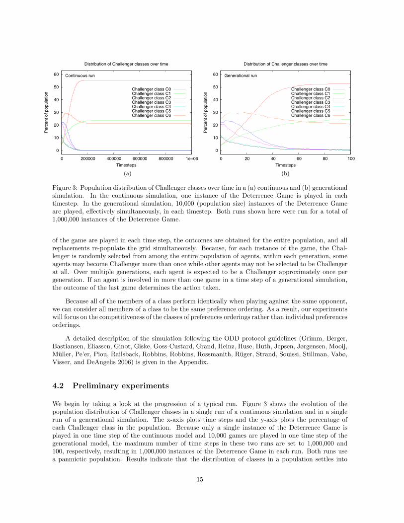
Figure 3: Population distribution of Challenger classes over time in a (a) continuous and (b) generationalsimulation. In the continuous simulation, one instance of the Deterrence Game is played in eachtimestep. In the generational simulation, 10,000 (population size) instances of the Deterrence Gameare played, effectively simultaneously, in each timestep. Both runs shown here were run for a total of1,000,000 instances of the Deterrence Game.

of the game are played in each time step, the outcomes are obtained for the entire population, and allreplacements re-populate the grid simultaneously. Because, for each instance of the game, the Chal-lenger is randomly selected from among the entire population of agents, within each generation, someagents may become Challenger more than once while other agents may not be selected to be Challengerat all. Over multiple generations, each agent is expected to be a Challenger approximately once pergeneration. If an agent is involved in more than one game in a time step of a generational simulation,the outcome of the last game determines the action taken.

Because all of the members of a class perform identically when playing against the same opponent,we can consider all members of a class to be the same preference ordering. As a result, our experimentswill focus on the competitiveness of the classes of preferences orderings rather than individual preferencesorderings.

A detailed description of the simulation following the ODD protocol guidelines (Grimm, Berger,Bastiansen, Eliassen, Ginot, Giske, Goss-Custard, Grand, Heinz, Huse, Huth, Jepsen, Jørgensen, Mooij,Muller, Pe’er, Piou, Railsback, Robbins, Robbins, Rossmanith, Ruger, Strand, Souissi, Stillman, Vabø,Visser, and DeAngelis 2006) is given in the Appendix.

4.2 Preliminary experiments

We begin by taking a look at the progression of a typical run. Figure 3 shows the evolution of thepopulation distribution of Challenger classes in a single run of a continuous simulation and in a singlerun of a generational simulation. The x-axis plots time steps and the y-axis plots the percentage ofeach Challenger class in the population. Because only a single instance of the Deterrence Game isplayed in one time step of the continuous model and 10,000 games are played in one time step of thegenerational model, the maximum number of time steps in these two runs are set to 1,000,000 and100, respectively, resulting in 1,000,000 instances of the Deterrence Game in each run. Both runs usea panmictic population. Results indicate that the distribution of classes in a population settles into

15

0

10

20

30

40

50

60

0 100 200 300 400 500

Perc

ent o

f pop

ulat

ion

Timesteps


Panmictic population


0

10

20

30

40

50

60

0 100 200 300 400 500

Perc

ent o

f pop

ulat

ion

Timesteps


Spatially-structured population


(a) (b)

Figure 4: Population distribution of Challenger classes over time in a generational simulation using a(a) panmictic and (b) spatially-structured population.

a stable state over time. The distribution at which a population settles appears to be independent ofwhether a simulation is continuous or generational. The continuous simulation requires fewer instancesof the Deterrence Game to settle down into a stable distribution.

We next examine whether the Defender selection method affects simulation results. Figure 4 showsthe evolution of the population distribution of Challenger classes in a single run using a panmicticpopulation and in a single run using a spatially-structured population. The x-axis plots time stepsand the y-axis plots the percentage of each Challenger class in the population. Both runs use thegenerational simulation structure. Preference orderings from class C0 are the most abundant in bothruns and stabilize at approximately the same level. The next most abundant classes of preferenceordering are C1 and C6. Using a panmictic population, class C1 stabilizes at a slightly higher levelthan class C6. Using a spatial population, class C6 stabilizes at a slightly higher level than class C1. Thisdifference remains and is statistically significant when the stabilized distribution of classes is averagedover 100 runs. The panmictic population reaches stability slightly faster than the spatially-structuredpopulation, due to the faster spread of information in a panmictic population.

4.3 Survival of preference orderings

The questions that we would like to answer are whether the preference orderings that survive in ouragent-based simulation will correlate with the survivability values from Tables 12 and 17 and whether thefive traditionally studied preference orderings will be among the survivors. To answer these questions,we run a series of experiments each consisting of 100 runs of the simulation. We take the distributionof Challenger and Defender classes from the last time step of each run and average these values overthe 100 runs. Each simulation is run for 1000 time steps which is sufficient to allow for the populationdistribution to stabilize. All runs use the generational simulation structure. We examine both panmicticand spatially-structured populations. In addition, we look at both actions for the war outcome, random-replace and random-winner.

Figure 5 shows the results of our first four sets of experiments. The results in the top row use therandom-replace action for war. The results in the bottom row use the random-winner action for war.The left two plots use a panmictic population. The right two plots use a spatially-structured population.

16

0

20

40

60

80

100

C0 C1 C2 C3 C4 C5 C6 D0 D1 D2 D3

Perc

ent o

f pop

ulat

ion

Panmictic populationWar action: random-replace

0

20

40

60

80

100

C0 C1 C2 C3 C4 C5 C6 D0 D1 D2 D3

Perc

ent o

f pop

ulat

ion

Spatially-structured populationWar action: random-replace

0

20

40

60

80

100

C0 C1 C2 C3 C4 C5 C6 D0 D1 D2 D3

Perc

ent o

f pop

ulat

ion

Panmictic populationWar action: random-winner

0

20

40

60

80

100

C0 C1 C2 C3 C4 C5 C6 D0 D1 D2 D3

Perc

ent o

f pop

ulat

ion

Spatially-structured populationWar action: random-winner

Figure 5: Population distribution of Challenger and Defender classes in time step 1000 averaged over 100runs. Challenger class proportions are relative to the Challenger population. Defender class proportionsare relative to the Defender population. Error bars indicate one standard deviation.

The x-axis for each plot indicates the class. The y-axis for each plot indicates the population percentageat which a class stabilizes, averaged over 100 runs. Error bars indicate one standard deviation. Althoughboth Challenger and Defender classes are plotted in the same plots, Challenger percentage values arecalculated relative to the Challenger population only and Defender percentage values are calculatedrelative to the Defender population only.

The top row of Figure 5 shows the results for the experiments using the random-replace war action.In both the panmictic and spatially-structured population, Challenger classes C0 (Resolute Defender),C1 (Irresolute Defender), and C6 dominate. These three classes correspond to the three classes with thehighest theoretical survival probability and are the only classes that will always survive (because theyonly encounter outcomes A and S). Classes C2-C5 do not survive at all in the population. Defenderclass D0 (which includes Resolute Defender) is the only defender class that survives. This correspondsto the theoretical analysis which finds that D0 has the highest survival probability of the Defenderclasses. Although the analysis of class C4 indicates potential survival of class D1 preference orderings,we suspect the lack of survival of class D1 is related to the lack of survival of class C4. Note that, forboth Challenger and Defender, there will be occasional instances of all classes due to selection by arandom-replace action.

17

Class εCC0 1.0C1 1.0C2 0.5/0.042∗

C3 0.0C4 0.5/0.042∗

C5 0.0C6 1.0

Table 18: Challenger class survival probabilities against only class D0 Defenders. ∗For classes C2 andC4, the two εC values reflect when the random-winner/random-replace actions are used.

The bottom row of Figure 5 shows the results for the experiments using the random-winner waraction. While the Defender class distribution remains the same, the Challenger class distributions aredifferent. Five of the seven Challenger classes stabilize at non-zero values. These five include thethree from above, plus C2 and C4. Surprisingly, class C2 (which includes Rogue Challenger) is themost dominant class despite having a survival probability less than classes C0, C1, and C6. Althoughpreference orderings from class C4 do survive in these experiments, their relative proportion in thepopulation appears to be too low to facilitate survival of class D1 Defenders. The two Challengerclasses that do not survive are the two classes with the lowest survival probabilities.

Although we see that, in general, classes with higher survival probabilities (e.g. C0, C1, C6, D0)survive in the simulation population and classes with lower survival probabilities (e.g. C3, C5, D2,D3) do not survive, the correlation between the survival probability of a class and its proportion in astabilized population is not clear. We believe that these differences in correlation are due in part to thefact that Tables 12 and 17 assume a uniform distribution of the twenty-four possible opponents. Asa result, these values are accurate predictors of the likelihood that a preference ordering will survivein the early stages of our simulation, because the initial population of agent preference orderings areuniformly distributed over all possible preference orderings. As the simulation progresses and agentsreplace each other, however, the distribution of preference orderings in the population is becomes lessand less uniform and these values become less accurate predictors of survival.

In all four experiments, the defender population stabilizes to primarily class D0 Defenders. Thus,Table 18, which gives Challenger survival probabilities when playing only class D0 Defenders, may bea more accurate predictor of Challenger survival in our experiments. In the experiments that use therandom-winner war action, the defender population eventually converges to only class D0 Defenders andthe values in Table 18 predict the disappearance of classes C3 and C5 and the survival of classes C2 andC4 (in addition to C0, C1, and C6). In the experiments that use the random-replace war action, becausethe random-replace mechanism results in a constant influx of randomly selected Defender preferenceorderings, the Defender population never completely converges to only class D0 Defenders. This influxmay be responsible in part for the inability of classes C2 and C4 to survive in the random-replace runs.

4.4 Equal starting proportions

We would like to understand why class C2 performs unexpectedly well in simulations that use therandom-winner action. We suspect that the initial distribution of classes may be a factor. Classes C0and C1 both contain only a single preference ordering each, while class C2 contains five preference order-ings. That means that a randomly initialized population will have approximately five times as many C2preference orderings as C0 and C1 preference orderings. Recall that the random-winner action randomly

18

Defender Class

D0 D1 D2 D3 εC

Challenger C0 S A S A 1.0

Class C1 S S A A 1.0

C2 W A W A 0.75/0.571∗

C3 C C A A 0.5

C4 W S W S 0.75/0.571∗

C5 C C S S 0.5

C6 S S S S 1.0

εD 0.857/0.786∗ 0.714 0.571/0.5∗ 0.429

Table 19: Outcome table and survival probabilities based on class instead of individual preference order-ings. ∗For classes C2, C4, D0, and D2, the εC and εD values reflect when the random-winner/random-replace actions are used.

chooses a winner from among the two players of a game, while the random-replace action replaces bothplayers with a randomly chosen preference ordering from among the twenty-four possible preferenceorderings. As a result, runs that use random-winner do not have the external infusion of preferenceorderings into the population that runs that use random-replace have. Consequently, the initial distri-bution of classes may affect the stable states that can be reached. In addition, because random-replaceselects randomly from among all twenty-four possible preference orderings, the replacement process isalso biased toward classes with large membership.

We rerun the previous four experiments starting with an equal distribution of classes in the initialpopulation. In addition to the initial population distribution, we also adjust random-replace so thatclasses have equal probability of being selected. Table 19 gives the outcome table and survival proba-bilities if we focus on classes instead of individual preference orderings. Survival probabilities are verysimilar to those calculated from the full outcome table. Figure 6 shows the new experimental results.As with Figure 5, the top row shows the results for random-replace; the bottom row, random-winner.The left column uses a panmictic population; the right column, spatially structured. All four Defenderclass distributions remain unchanged: class D0 is clearly dominant. The Challenger class distributionsusing random-replace are also similar to those from Figure 5, except for a slight increase in the amountof classes C0 and C1 and decrease in the amount of class C6.

The Challenger class distributions for random-winner are noticeably different from those in Figure 5indicating that initial population distribution is a relevant factor. When the initial population startswith equal class distributions, classes C0, C1, and C2 are the most dominant, with class C1 having aslight edge over the other two. Classes C4 and C6 also stabilize at non-zero values and classes C3 and C5do not survive in the population at all. Although these results more closely match the expected survivalprobabilities than the random-winner results from Figure 5, some differences still exist. For example,class C6 has a higher survival probability than classes C2 and C4 but stabilizes at approximately thesame value as C4 and significantly less than C2 in the simulation. In addition, it is unclear why classC1 preference orderings are the most successful preference orderings in these runs.

4.5 Changing the Defender pool

One result that has remained constant throughout all of our experiments is the stabilized distribution ofDefender classes. Class D0 preference orderings, which include Resolute Defender, are always the only

19

0

20

40

60

80

100

C0 C1 C2 C3 C4 C5 C6 D0 D1 D2 D3

Perc

ent o

f pop

ulat

ion


0

20

40

60

80

100

C0 C1 C2 C3 C4 C5 C6 D0 D1 D2 D3

Perc

ent o

f pop

ulat

ion


0

20

40

60

80

100

C0 C1 C2 C3 C4 C5 C6 D0 D1 D2 D3

Perc

ent o

f pop

ulat

ion


0

20

40

60

80

100

C0 C1 C2 C3 C4 C5 C6 D0 D1 D2 D3

Perc

ent o

f pop

ulat

ion


Figure 6: Population distribution of Challenger and Defender classes in time step 1000 averaged over 100runs. The initial population starts with an equal distribution of both Challenger and Defender classes.Challenger class proportions are relative to the Challenger population. Defender class proportions arerelative to the Defender population. Error bars indicate one standard deviation.

ones that survive. Figure 7 shows the evolution of Defender classes in a typical run from Figures 5 and 6.Class D0 takes over early in the run and, for most of the run, is the only class of Defender preferenceorderings in the player pool. As a result, the Challenger preference orderings in our population areactually evolving to play against only the preference orderings from class D0, not all defender preferenceorderings.

We rerun the four experiments again with class D0 completely removed from the player pool to seehow this change affects the evolution of both Challenger and Defender classes. Initial populations startwith equal distributions of classes. In addition to eliminating class D0 preference orderings from theinitial population, they are also omitted from the random-replace operator. Table 20 gives the outcometable and survival probabilities if class D0 is removed. Figure 8 shows the resulting class distributionswhen class D0 preference orderings are eliminated from the simulations. As before, the top row showsthe results for random-replace; the bottom row, random-winner. The left column uses a panmicticpopulation; the right column, spatially structured.

In the simulations that use the random-replace operator, the removal of class D0 allows classes D1and D2 to thrive. The success of class D1 is not surprising because it has the next highest survival

20

0

20

40

60

80

100

0 200 400 600 800 1000

Perc

ent o

f pop

ulat

ion

Timesteps

Distribution of Defender classes over time

Defender class D0Defender class D1Defender class D2Defender class D3

Figure 7: Population distribution of Defender classes over time.

Defender Class

D1 D2 D3 εC

Challenger C0 A S A 1.0

Class C1 S A A 1.0

C2 A W A 0.833/0.714∗

C3 C A A 0.667

C4 S W S 0.833/0.714∗

C5 C S S 0.667

C6 S S S 1.0

εD 0.714 0.571/0.5∗ 0.429

Table 20: Outcome table and survival probabilities when class D0 is removed. ∗For classes C2, C4, andD2, the εC and εD values reflect when the random-winner/random-replace actions are used.

probability after class D0. Class D2, however, has a noticeably lower survival probability but similarsuccess as class D1. In the Challenger classes, classes C0 and C1 are the only survivors. Unlikethe previous experiments, class C6 is unable to survive in these runs. Classes C0, C1, and C6 haveidentically high survival probabilities. Clearly, then, class C6 preference orderings are dependent onclass D0 preference orderings for survival. In the simulations that use the random-winner operator,classes D1 and D2 once again thrive as Defender preference orderings. Surviving Challenger preferenceorderings include classes C0, C1, and C2. Once again, class C6 appears unable to survive without classD0. As with the simulations from Figure 6, it is unclear why class C1 is the most successful class inthese runs.

21

0

20

40

60

80

100

C0 C1 C2 C3 C4 C5 C6 D0 D1 D2 D3

Perc

ent o

f pop

ulat

ion


0

20

40

60

80

100

C0 C1 C2 C3 C4 C5 C6 D0 D1 D2 D3

Perc

ent o

f pop

ulat

ion


0

20

40

60

80

100

C0 C1 C2 C3 C4 C5 C6 D0 D1 D2 D3

Perc

ent o

f pop

ulat

ion


0

20

40

60

80

100

C0 C1 C2 C3 C4 C5 C6 D0 D1 D2 D3

Perc

ent o

f pop

ulat

ion


Figure 8: Population distribution of Challenger and Defender classes in time step 1000 averaged over100 runs. Class D0 preference orderings are completely omitted from the simulations. The initialpopulation starts with an equal distribution of active Challenger and Defender classes. Challenger classproportions are relative to the Challenger population. Defender class proportions are relative to theDefender population. Error bars indicate one standard deviation.

4.6 Importance of player pool on class survival

Why would the number of preference orderings from class C6 go to zero when the theoretical analysisindicates that preference orderings from class C6 will always survive a game? Class C6 challengersprefer S (status quo) over all other outcomes. As a result, they never initiate a challenge thus ensuringtheir survival. C6 preference orderings may be lost if their partner defender preference orderings lose agame, but it seems unlikely that all C6 preference orderings would consistently be lost in this way. Tobetter understand what is happening, we begin by examining the class distributions within individualruns from the results shown in Figures 6 (equal starting proportions for all classes including D0) and 8(equal starting proportions without class D0). The observed evolution of class distributions withinindividual runs leads us to a re-examination of the data in Table 19 which illustrates how the playerpool can affect survival of classes.

Figure 9 shows the evolution of the population distribution of both challenger and defender classesover time from a sample run in which all classes are initialized in equal proportions (from the data from

22

0

10

20

30

40

50

60

70

80

90

100

0 200 400 600 800 1000

Perc

ent o

f pop

ulat

ion

Timesteps


C0C1C2C3C4C5C6D0D1D2D3

0

10

20

30

40

50

60

70

80

90

100

0 200 400 600 800 1000

Perc

ent o

f pop

ulat

ion

Timesteps



0

10

20

30

40

50

60

70

80

90

100

0 200 400 600 800 1000

Perc

ent o

f pop

ulat

ion

Timesteps



0

10

20

30

40

50

60

70

80

90

100

0 200 400 600 800 1000

Perc

ent o

f pop

ulat

ion

Timesteps



Figure 9: Distribution of classes in the population in each timestep of a sample run when all classes areinitialized in equal proportions. Challenger class proportions are relative to the Challenger population.Defender class proportions are relative to the Defender population.

Figure 6). Figure 10 shows the evolution of the population distribution from a sample run in which allclasses minus class D0 are initialized in equal proportions (from the data from Figure 8). The x-axis plotstime steps and the y-axis plots the percentage of each class. Challenger and defender percentages arecalculated independently; that is, all challenger percentages sum to 100% and all defender percentagessum to 100%.

The most striking difference between the results shown in Figures 9 and 10 is the stability of theclass distributions. When class D0 preference orderings are included in the population (Figure 9), itbecomes the dominant defender preference ordering in the population. We believe that the fact thata single defender opponent dominates the population allows the challenger class proportions, and theentire system, to settle down into a relatively stable distribution. If we consider the leftmost column ofTable 19 which lists the games and outcomes4 that occur when class D0 preference orderings dominate

4Recall that an outcome of S means that both Challenger and Defender are unchanged, ensuring the survival of thepreference orderings of both Challenger and Defender. An outcome of C means that Challenger will be replaced byDefender. Unless both Challenger and Defender have identical preference orderings, Challenger’s preference orderings (forboth defender and challenger roles) will decrease in the population and Defender’s preference orderings will increase. Anoutcome of A means that Defender will be replaced by Challenger which means that Challenger’s preference orderingswill increase in the population and Defender’s preference orderings will descrease. An outcome of W results in a non-zero

23

0

10

20

30

40

50

60

70

0 200 400 600 800 1000 1200

Perc

ent o

f pop

ulat

ion

Timesteps



0

10

20

30

40

50

60

70

0 200 400 600 800 1000 1200

Perc

ent o

f pop

ulat

ion

Timesteps



0

10

20

30

40

50

60

70

0 200 400 600 800 1000 1200

Perc

ent o

f pop

ulat

ion

Timesteps



0

10

20

30

40

50

60

70

0 200 400 600 800 1000 1200

Perc

ent o

f pop

ulat

ion

Timesteps



Figure 10: Distribution of classes in the population in each timestep of a sample run when all classesminus class D0 are initialized in equal proportions. Class D0 preference orderings are completely omittedfrom the simulations. Challenger class proportions are relative to the Challenger population. Defenderclass proportions are relative to the Defender population.

the population, we see that three outcomes are possible: S, W, and C. In the random-replace experimentsin which W outcomes provide the population with an influx of random preference orderings (left columnof Figure 9), the challenger classes with non-trivial survival proportions are C0, C1, and C6: exactlythose classes that Table 19 indicates will have the highest survival probabilty against D0 via the Soutcome. The difference in their proportions is likely a result of the early games in the run, whenother defender preference orderings are still present in the population in significant numbers. In therandom-winner experiments where W outcomes do not provide the population with a random influx ofpreference orderings (right column of Figure 9), challenger classes whose outcomes against D0 are Walso survive. The relative proportions of the surviving challenger classes differ from the proportions inthe random-replace experiments, which is most likely due to the lack of input of new classes into thepopulation from the random-winner action.

When class D0 preference orderings are excluded from the population, Figure 10 reveals a dynamicthat is not evident in Figure 8. Instead of stabilizing to a steady value, the various classes of preference

probability of survival for both Challenger and Defender. This probability is less than the guaranteed survival offered bythe S outcome.

24

orderings appear to activate and inhibit each other resulting in regular oscillations in their relativeproportions in the population. Specifically, in the random-replace experiments (left column of Figure 10),the growth of class D1 in the population appears to stimulate the growth class C0. When the proportionof class C0 grows, the proportion of other challenger classes must decrease. Class C0, in turn, activatesD2 (which inhibits D1); class D2 activates C1 (which inhibits C0); and class C1 activates D1 (whichinhibits D2). Then the cycle starts all over again. The observed oscillations and inability to stabilizeappear to be due to the fact that neither side converges to a single dominant preference ordering andthe mixed distributions on both sides result in a constantly changing environment in which differentclasses excel.

Once again, the details in Table 19 provide an explanation of what is happening. When class D0is excluded from the defender pool, both class D1 and D2 are able to survive. Because class D1 has ahigher survival probability, we will assume that it initially grows (increases its proportion) faster in thepopulation than class D2. Examination of the plots in Figure 10 support this assumption. Columnstwo and three of Table 19 list the outcomes for games involving class D1 and D2 preference orderings.For each challenger class, if we consider the pair of outcomes that involve D1 and D2 and if we assumethat D1 initially grows faster in the population and, consequently, column two has a greater effect, wefind that class C0 has the highest potential for growth (many A outcomes due to D1’s growth, some Soutcomes due to D2). Class C1 has the next highest potential (some A outcomes, many S outcomes).The remaining challenger classes have little to no potential for growth. As a result, D1 activates C0and D2 maintains C1 in the population. If we then consider rows one and two of Table 19 which listthe outcomes for games involving class C0 and C1 preference orderings, we find that a high proportionof C0 activates D2 and a moderate proportion of C2 maintains D1 in the population. Continuing withthis analysis, a high proportion of D2 activates C1 and a moderate proportion of D1 maintains C0. Ahigh proportion of C1 activates D1 and a moderate proportion of C0 maintains C2. Then the cyclestarts over again. The order in which classes are activated in this analysis matches the order in whichclasses are activated in the random-replace experiments in Figure 10.

In the random-winner experiments (right column of Figure 10), similar oscillations are observedand the number and proportions of surviving classes differ from that of the random-replace experiments.Once again, we believe the differences and more complex interactions to be due to the fact that therandom-winner populations receive no external influx of new preference orderings.

5 Discussion

Agent-based simulations have been used to study many different types of social systems in which multipleplayers or agents interact over time (Axelrod 1997; Cioffi-Revilla 2010a; Cioffi-Revilla 2010b; Epsteinand Axtell 1996; Epstein 2006). Where traditional equation-based models focus on the relationshipamong the observable characteristics of a system, agent-based models focus on the interactions of theindividual agents that make up a system and, thus, may yield different insights into system and agentdynamics (Parunak, Savit, and Riolo 1998).

We use an agent-based simulation consisting of a population of competing agents to examine therelative strengths of all possible preference orderings for the Deterrence Game. Stronger preferenceorderings are expected to survive in the population while weaker ones die out. As a result, we cancompare the stabilized distribution of preference orderings from the simulation with the estimatedsurvival probabilities given in Tables 12 and 17.

Our results show that preference orderings with higher survival probabilities are more likely tosurvive in the simulation population, but the relative distribution of preference orderings at which the

25

simulation population stabilizes is not always proportional to the relative survival probabilities. Webelieve that this is due in part to the fact that the estimated survival probabilities given in Tables 12and 17 assume a fixed probability of encountering each opponent, calculated from the initial populationdistribution. As a result, these values are likely to be more accurate early in a run when the populationdistribution is similar to the values used in the calculations, but less accurate later in a run as thepopulation distributions change over time.

Two factors appear to have a significant effect on the distributions at which populations stabilizeand the classes that survive: the initial population distribution and the player pool.

1. The initial population distribution refers to the relative proportions of each class found in theinitial population. Because the seven Challenger classes and four Defender classes vary in the sizeof their membership, when a population is initialized randomly using all twenty-four preferenceorderings, some classes will be present in higher proportions than others. Changing the simulationsuch that all classes are equally represented in the initial population changes the final distributionof classes at which the population stabilizes. Thus, the initial state of the system can affect thestate at which the system stabilizes.

2. Player pool refers to the preference orderings that are available to play in a population. Addingor removing players from the pool can significantly change the resulting distribution of classes atpopulation stabilization. Removing a strong player, such as Resolute Defender, not only allowsother defender classes to survive in the population, but also changes the surviving Challengerclasses and distributions as well. In other words, who wins depends in part on who plays thegame. This effect has been observed in other population based models (Axelrod 1980a; Axelrod1980b; Dacey and Pendegraft 1988; Dacey and Pendegraft 1990), and is due to the fact that theplayer pool defines the environment in which the agents interact and different preference orderingsmay survive in different environments.

Our simulation shows that variation in the rate at which the population distribution and playerpool change in the system can have a significant effect on which preference orderings survive. The factthat the initial population distribution affects the final population suggests that the relative time ittakes for a class to die out can affect the evolutionary trajectory of a population (Dacey and Pendegraft1990). As members of a class are lost, the population distribution changes; eventually, when an entireclass is lost, the player pool changes. The fact that the player pool can significantly affect the survivaland distribution of classes reinforces the notion that knowledge of one’s opponent or opponents as wellas knowledge of oneself are essential in preparations for situations of conflict (Galvin 2003).

6 Conclusions

The Deterrence Game is a two player game where each player has two possible actions and the players’interaction results in one of four possible outcomes. Players are defined by their preference orderings overthese four outcomes; as a result, twenty-four unique preference orderings are possible. Of the twenty-fourpossible preference orderings, only five are seriously studied in the deterrence literature. Examination ofthe table of all possible outcomes finds that many preference orderings behave identically and there areonly seven classes of Challenger preference orderings and four classes of Defender preference orderings.Because all of the preference orderings in a class behave identically with respect to all possible opponents,for all practical purposes, all preference orderings within each class are equivalent. We define a measureof survival and calculate the probability of survival for each preference ordering class. In addition, weidentify the defining characteristics of each preference ordering class.

26

We implement an agent-based computer simulation to empirically test the survival of preferenceorderings in a population of interacting agents. The simulation may be run in either continuous orgenerational mode. The population may be either panmictic or spatially-structured. Over time, thepopulation in a run will stabilize to a fixed distribution of preference ordering classes. We use therelative stabilization values as a measure of the competitiveness of each class.

The goals of this paper are to answer three questions: are the five traditionally studied DeterrenceGame preference orderings the most competitive for their roles, are there other preference orderingsthat are competitive in the Deterrence Game, and what are the characteristics that make a preferenceordering competitive or uncompetitive?

Of the five traditionally studied preference orderings, three – Resolute Challenger, Irresolute Chal-lenger, and Resolute Defender – consistently survive in the agent-based simulations. While ResoluteChallenger and Irresolute Challenger exhibit unique behaviors and are the sole members of their corre-sponding classes, Resolute Defender is a member of a larger class containing other preference orderingswith identical behaviors. These equivalent preference orderings also consistently survive in the agent-based simulations. Rogue Challenger and its class of equivalent preference orderings perform well onlywhen populations are limited to their initial memberships and there is no external infusion of newpreference orderings. Irresolute Defender and its class of equivalent preference orderings are able tosurvive only when the Resolute Defender class is eliminated from the player pool. The characteristicsthat are common to the surviving (and non-surviving) classes of players are summarized in Tables 12and 17. Additional factors that affect the preference orderings that survive to a final stable populationinclude the initial population distribution and the player pool.

Appendix: ODD protocol

The following is a description of our simulation system following the ODD protocol guidelines (Grimm,Berger, Bastiansen, Eliassen, Ginot, Giske, Goss-Custard, Grand, Heinz, Huse, Huth, Jepsen, Jørgensen,Mooij, Muller, Pe’er, Piou, Railsback, Robbins, Robbins, Rossmanith, Ruger, Strand, Souissi, Stillman,Vabø, Visser, and DeAngelis 2006).

6.1 Overview

6.1.1 Purpose

The purpose of this system is to provide an agent-based platform on which we can examine the relativesurvivability of of Challenger and Defender preference orderings in the Traditional Deterrence Game inboth spatial and non-spatial settings.

This simulation is written in C and compiled using the gcc compiler.

6.1.2 State variables and scales

The simulation consists of a single type of agent. Agents reside on a toroidal two-dimensional gridcalled grid. Each cell of the grid holds a single agent. Each agent is referenced by its location, e.g. theagent in row x and column y of grid is called grid(x, y). Agent parameters are given in Table 21.

27

PseudocodeParameter Description VariableChallenger preference A character indicating one of the 24 possible c prefordering preference orderings. This is the preference

ordering that the agent uses when it plays theDeterrence Game in the Challenger role.

Defender preference A character indicating one of the 24 possible d prefordering preference orderings. This is the preference

ordering that the agent uses when it plays theDeterrence Game in the Defender role.

Table 21: Agent parameters.

6.1.3 Process overview and scheduling

Time is modeled in discrete time steps. The simulation can be run in two modes, continuous andgenerational.

In continuous mode, one instance of the Deterrence Game is played in each timestep and theoutcome action is applied immediately. The pseudocode in Algorithm 1 defines what happens in acontinuous mode simulation.

In generational mode, popsize instances of the Deterrence Game are played, essentially in parallel,in each timestep and all outcome actions are applied simultaneously. Because the Challenger is selectedrandomly for each instance of the Deterrence Game, within each timestep, some agents may be selectedto be Challenger more than once and some agents may not be selected at all. Over multiple timesteps,each agent is expected to be a Challenger approximately once per timestep.

From an implementation perspective, this means that an additional temporary grid, tempgrid mustbe used. For each instance of the Deterrence Game played in each timestep, players are selected fromthe original grid, grid, and the agents that result are stored in the corresponding locations in tempgrid.At the end of each timestep, all agents from tempgrid are copied to grid, representing the simultaneousapplication of all outcome actions. The pseudocode in algorithms 2 and 3 define what happens in agenerational mode simulation.

6.2 Design concepts

Adaptation: The outcome of a Deterrence game determines whether and how the player agents willadapt their c pref and d pref preference orderings. Outcome actions are defined in Table 5.

Sensing: When selected to play the Deterrence game, agents are able to sense their own preferenceorderings and the preference orderings of their opponent.

Stochasticity: Stochasticity is present in three aspects of the simulation: (1) population initial-ization, (2) in the player selection process, and (3) in the actions that are performed in the event of aWar outcome. In the population initialization and player selection processes, stochasticity eliminatesbiases that may emerge from agents’ relative locations. In the actions performed for a War outcome,stochasticity is utilized to represent the unpredictability of the War outcome.

Observation: The distribution of preference orderings in the population in each timestep is col-

28

Algorithm 1 Continuous mode simulation

1: procedure Continuous Mode Simulation2: Initialize grid with one agent per cell, each with a randomly assigned c pref and d pref value3: for timestep← 1,max timestep do4: agentC ← randomly choose one agent from population . Choose Challenger5: if panmictic population then . Choose Defender6: agentD ← randomly choose one agent from population7: else if spatially-structured population then8: agentD ← randomly choose one of the eight adjacent neighbors of agentC9: end if

10: outcome← Play Deterrence game(agentC , agentD) . Play Deterrence Game11: if outcome = Acquiesce then . Apply action based on game outcome12: agentD.c pref ← agentC .c pref13: agentD.d pref ← agentC .d pref14: else if outcome = Capitulate then15: agentC .c pref ← agentD.c pref16: agentC .d pref ← agentD.d pref17: else if outcome = War then18: if random-winner then19: winner ← randomly choose a winner between agentC and agentD20: if winner = agentC then21: agentD.c pref ← agentC .c pref22: agentD.d pref ← agentC .d pref23: else if winner = agentD then24: agentC .c pref ← agentD.c pref25: agentC .d pref ← agentD.d pref26: end if27: else if random-replace then28: agentC .c pref ← randomly choose one of the 24 possible preference orderings29: agentC .d pref ← randomly choose one of the 24 possible preference orderings30: agentD.c pref ← randomly choose one of the 24 possible preference orderings31: agentD.d pref ← randomly choose one of the 24 possible preference orderings32: end if33: end if34: end for35: end procedure

lected for analysis.

6.3 Details

6.3.1 Initialization

The simulation consists of a two-dimensional grid with one agent in each cell of the grid. Each agent hasa Challenger preference ordering and a Defender preference ordering. At the start of the simulation,agents are randomly assigned one of 24 possible preference ordering for their Challenger preferenceordering and one of 24 possible preference ordering for their Defender preference ordering.

29

Algorithm 2 Generational mode simulation

1: procedure Generational Mode Simulation2: Initialize grid with one agent per cell, each with a randomly assigned c pref and d pref value3: popsize← numrows ∗ numcols4: for timestep← 1,max timestep do5: Copy Grid(tempgrid, grid) . Copy grid to tempgrid6: for subtimestep← 1, popsize do7: xC ← random integer between 1 and numrows, inclusive . Challenger is agent8: yC ← random integer between 1 and numcols, inclusive . at grid(xC , yC)9: if panmictic population then

10: xD ← random integer between 1 and numrows, inclusive . Defender is agent11: yD ← random integer between 1 and numcols, inclusive . at grid(xD, yD)12: else if spatially-structured population then13: xD ← random integer between xC − 1 and xC + 1, inclusive14: yD ← random integer between yC − 1 and yC + 1, inclusive15: end if16: outcome← Play Deterrence game(grid(xC , yC), grid(xD, yD))17: if outcome = Acquiesce then . Apply actions to tempgrid18: tempgrid(xD, yD).c pref ← grid(xC , yC).c pref19: tempgrid(xD, yD).d pref ← grid(xC , yC).d pref20: else if outcome = Capitulate then21: tempgrid(xC , yC).c pref ← grid(xD, yD).c pref22: tempgrid(xC , yC).d pref ← grid(xD, yD).d pref23: else if outcome = War then24: if random-winner then25: winner ← randomly choose a winner between grid(xC , yC) and grid(xD, yD)26: if winner = grid(xC , yC) then27: tempgrid(xD, yD).c pref ← grid(xC , yC).c pref28: tempgrid(xD, yD).d pref ← grid(xC , yC).d pref29: else if winner = grid(xD, yD) then30: tempgrid(xC , yC).c pref ← grid(xD, yD).c pref31: tempgrid(xC , yC).d pref ← grid(xD, yD).d pref32: end if33: else if random-replace then34: tempgrid(xC , yC).c pref ← randomly choose one of 24 possible pref. orderings35: tempgrid(xC , yC).d pref ← randomly choose one of 24 possible pref. orderings36: tempgrid(xD, yD).c pref ← randomly choose one of 24 possible pref. orderings37: tempgrid(xD, yD).d pref ← randomly choose one of 24 possible pref. orderings38: end if39: end if40: end for41: Copy Grid(grid, tempgrid) . Copy tempgrid to grid42: end for43: end procedure

30

Algorithm 3 Copy grid

1: procedure Copy Grid(gridA, gridB)2: for x← 1, numrows do3: for y ← 1, numcols do4: gridA(x, y)← gridB(x, y)5: end for6: end for7: end procedure

6.3.2 Input

Other than system initialization, the simulation receives no external input during a run.

6.3.3 Submodels

All algorithm details are included in the pseudocode in Algorithms 1-3. The dynamics of the DeterrenceGame are illustated in Figure 1 and the outcomes for every possible pair of players are given in Table 4.

References

Axelrod, R. (1980a). Effective choice in the Prisoner’s Dilemma. Journal of Conflict Resolution 24 (1),3–25.

Axelrod, R. (1980b). More effective choice in the Prisoner’s Dilemma. Journal of Conflict Resolu-tion 24 (3), 379–403.

Axelrod, R. (1997). The Complexity of Cooperation. Princeton University Press.

Barbot, C., O. Betancor, M. P. Socorro, and M. F. Viecens (2014). Trade-offs between environmentalregulation and market competition: Airlines, emission trading systems and entry deterrence.Transport Policy 33, 65–72.

Brams, S. J. and C. M. Kilgour (1985). Optimal deterrence. Social Philosophy and Policy 3 (1),118–135.

Carlson, L. J. and R. Dacey (2006). Sequential analysis of deterrence games with a declining statusquo. Conflict Management and Peace Science 23, 181–198.

Carlson, L. J., R. Dacey, R. B. Heckendorn, and A. S. Wu (2008). Computational modeling ofthe traditional deterrence game. In International Studies Association 49th Annual Conference:Bridging Multiple Divides, pp. 1–23.

Cioffi-Revilla, C. (2010a). Computational social science. Wiley Interdisciplinary Reviews: Computa-tional Statistics 2 (3), 259–271.

Cioffi-Revilla, C. (2010b). A methodology for complex social simulations. Journal of Artificial Soci-eties and Social Simulation 13 (1).

da Cruz, J. F., H. Gaspar, and G. Calado (2012). Turning the game around: toxicity in a nudibranch-sponge predator prey association. Chemoecology 22 (1), 47–53.

Dacey, R. and N. Pendegraft (1988). The optimality of tit-for-tat. International Interactions 15 (1),45–64.

31

Dacey, R. and N. Pendegraft (1990). The impact of election frequency and crises upon the arms race.International Interactions 15 (3/4), 331–343.

Durlauf, S. N., C. Fu, and S. Navarro (2013). Capital punishment and deterrence: Understandingdisparate results. Journal of Quantitative Criminology 29 (1), 103–121.

Ellsberg, D. (1961). The crude analysis of strategic choices. American Economic Review 51 (2), 472–478.

Epstein, J. M. (2006). Generative Social Science: Studies in Agent-based Computational Modeling.Princeton University Press.

Epstein, J. M. and R. Axtell (1996). Growing Artificial Societies: Social Science from the BottomUp. Brookings Institution Press.

Galvin, D. (2003). Sun Tzu: The Art of War. New York: Barnes and Noble Classics. (Edited by D.Galvin. Translated by L. Giles.).

Grimm, V., U. Berger, F. Bastiansen, S. Eliassen, V. Ginot, J. Giske, J. Goss-Custard, T. Grand,S. K. Heinz, G. Huse, A. Huth, J. U. Jepsen, C. Jørgensen, W. M. Mooij, B. Muller, G. Pe’er,C. Piou, S. F. Railsback, A. M. Robbins, M. M. Robbins, E. Rossmanith, N. Ruger, E. Strand,S. Souissi, R. A. Stillman, R. Vabø, U. Visser, and D. L. DeAngelis (2006). A standard protocolfor describing individual-based and agent-based models. Biological Modelling 198, 115–126.

Huth, P. K. (1999). Deterrence and international conflict: Empirical findings and theoretical debates.Annual Review of Political Science 2 (1), 25–48.

Jervis, R. (1979). Deterrence theory revisited. World Politics 31 (2), 289–324.

Johnson, J. C., B. A. Leeds, and A. Wu (2015). Capability, credibility, and extended general deter-rence. International Interactions 41 (2), 309–336.

Kagan, M. (2016). Limiting deterrence: Judicial resistance to detention of asylum-seekers in Israeland the United States. Texas International Law Journal 51 (2/3), 191–211.

Langlois, J.-P. P. and C. C. Langlois (2005). Fully informed and on the road to ruin: The perfectfailure of asymmetric deterrence. International Studies Quarterly 49, 503–527.

Misra, A. K. (2014). Modeling the effect of police deterrence on the prevelance of crime in the society.Applied Mathematics and Computation 237, 531–545.

Modongal, S. (2016). Deterrence of nuclear terrorism in the context of South Asia. Defense andSecurity Analysis 32 (2), 192–198.

Mooijman, M., W. W. van Dijk, N. Ellemers, and E. van Dijk (2015). Why leaders punish: A powerperspective. Journal of Personality and Social Psychology 109 (1), 75–89.

Morgan, P. M. (1977). Deterrence. Sage Publications.

Morrow, J. D. (1994). Game Theory for Political Scientists. Princeton University Press.

Nalebuff, B. (1991). Rational deterrence in an imperfect world. World Politics 43 (3), 313–335.

Ossa, R. (2014). Trade wars and trade talks with data. The American Economic Review 104 (12),4104–4146.

Pantaleo, G., A. M. Miron, M. A. Ferguson, and S. D. Frankowski (2014). Effects of deterrence on in-tensity of group identification and efforts to protect group identity. Motivation and Emotion 38 (6),855–865.

Parunak, H. V. D., R. Savit, and R. L. Riolo (1998). Agent-based modeling vs. equation-basedmodeling: A case study and users’ guide. In Multi-Agent Systems and Agent-Based Simulation,LNAI 1534, pp. 10–25. Springer Berlin Heidelberg.

Payne, K. B. (2015). US nuclear weapons and deterrence. Air and Space Power Journal 29 (4), 63–71.

32

Powell, R. (1990). Nuclear Deterrence Theory: The Search for Credibility. Cambridge UniversityPress.

Russett, B. M. (1963). The calculus of deterrence. Journal of Conflict Resolution 7 (2), 97–109.

Ruxton, G. D., T. N. Sherratt, and M. P. Speed (2004). Avoiding Attack: The evolutionary ecologyof crypsis, warning signals and mimicry. Oxford University Press.

Scheber, T. (2011). Evolutionary psychology, cognitive function, and deterrence. Comparative Strat-egy 30 (5), 453–480.

Schelling, T. C. (1966). Arms and Influence. Yale University Press.

Simon, M. W. (2002). Rogue state response to BMD: The regional context. Defense and SecurityAnalysis 18 (3), 271–292.

Wang, S. and Y. Wang (2016). Transition of interactions between a cuckoo and its host: Fluctuatingbetween parasitism and mutualism. Applied Mathematics and Computation 273, 664–677.

Zagare, F. C. (1987). The Dynamics of Deterrence. The University of Chicago Press.

Zagare, F. C. and D. M. Kilgour (1993). Asymmetric deterrence. International Studies Quarterly 37,1–27.

Zagare, F. C. and D. M. Kilgour (2000). Perfect Deterrence. Cambridge University Press.

33

Evolution of preference orderings for the Deterrence …ecl/papers/1709.cs-tr-17-04.pdfEvolution of...

Documents

Transcript of Evolution of preference orderings for the Deterrence …ecl/papers/1709.cs-tr-17-04.pdfEvolution of...