Evolution of performance of an automotive wind tunnel · PDF fileEvolution of performance of...

ARTICLE IN PRESS

Journal of Wind Engineering

and Industrial Aerodynamics 96 (2008) 667–700

0167-6105/$ -

doi:10.1016/j

E-mail ad

www.elsevier.com/locate/jweia

Evolution of performance of an automotivewind tunnel

A. Cogotti

Former Director of the Aerodynamic and Aeroacoustic Research Center, Pininfarina S.p.A, Turin, Italy

Abstract

The continuous evolution in the automotive world demands a parallel evolution in the facilities

and in the measuring techniques. The paper describes the evolution of the automotive wind tunnel in

Pininfarina as well as the progress made in parallel to its measuring techniques. Eventually, the paper

reports examples of the measurements made with these techniques during the aerodynamic and

aeroacoustic development of new cars.

r 2008 Published by Elsevier Ltd.

Keywords: Aerodynamics; Aeroacoustics; Wind tunnel; Cars

1. Introduction

The evolution of passenger cars, in the last years, has been extremely fast because ofincreased competition between the car companies. In order to cope with this evolution, acontinuous improvement of the testing facility and of the measuring techniques isnecessary. In fact the technical requirements for the new car models are usually more andmore stringent, in any case never lower than the previous ones. Furthermore, the availabletime for the development tends to be more and more reduced, in order to reach a shortertime-to-market.

In addition to all that, also the number of prototypes which are available for the testsduring the development phase, tends to be reduced for cost reasons. To fulfill all thesedifferent requirements, it is necessary to develop new measuring techniques that arecapable of investigating and understanding, in a short time, the aerodynamic and the

see front matter r 2008 Published by Elsevier Ltd.

.jweia.2007.06.007

dress: [email protected]

www.elsevier.com/locate/jweia

dx.doi.org/10.1016/j.jweia.2007.06.007

mailto:[email protected]

ARTICLE IN PRESSA. Cogotti / J. Wind Eng. Ind. Aerodyn. 96 (2008) 667–700668

aeroacoustic flow field in every detail. In this way it is possible to find the most appropriatesolutions and to fix the problems that are found during the development. At the same time,it is fundamental to improve the testing facility, where the development is carried out, so asto make it as close as possible to the road. This means that the flow conditions in the testsection have to be as representative as possible to those existing on the road.All that to prevent the development of solutions that could be optimal in the wind tunnel

but less effective on the road: that would involve additional costs without giving realbenefits.Keeping in mind all that, the strategy of Pininfarina has continuously been focused

towards these two main targets:

(a)
improvement of the measuring techniques (b) upgrading the facility performance
In the first case, new measuring techniques were developed so as to be able to investigatein a short time the details of the aerodynamic and aeroacoustic flow field.In the second case, a number of modifications were carried out to the facility in order to:

�
reduce the ambient noise to improve aeroacoustic measurements. � simulate in the wind tunnel the relative motion between the car and the ground, as well
as the rotation of the car wheels and that is necessary to improve the flow simulationalong the underbody, in the wheels/wheelhousings areas and more generally in most ofthe car flow field.
� generate, when needed, a suitable turbulent flow so as to reproduce the conditions that a
car finds on the road in the presence of ambient wind.

All these aspects are described in detail in the following paragraphs. More details can befound in some papers that deal specifically with these topics and that are listed in thereferences.It is worth outlining that some improvements made to the measuring techniques are

dependent on the upgrades carried out to the flow simulation in the wind tunnel. Inparticular the turbulence generation system (TGS) produces a flow condition that isunsteady and therefore time dependent. So, to investigate in an appropriate way theseflows, it is necessary to use more advanced measuring techniques that are able to maketime-resolved measurements. See Sections 3.4, 3.5 and 3.7 as examples of techniques thatare appropriate to investigate unsteady flows.

2. Facility upgrading

Construction of the Pininfarina full-scale automotive wind tunnel was over in 1972 and,after a period of commissioning, was put into operation in 1973. It was the first in Italy andone of the first in Europe. Its performance, compared to present day standards, is certainlypoor. At that time, it was common practice to carry out the tests with ground fixed andwheels static.Furthermore, it was accepted that the ambient noise in the wind tunnel was pretty high,

as the aeroacoustic noise of passenger cars was not yet an issue (Fig. 1).

ARTICLE IN PRESS

Fig. 1. A view of the original wind tunnel, as built in 1972. Typical features, the high-noise fan, the static ground

and the absence of acoustic treatment on the plenum walls.

Fig. 2. (a) First major improvements made in 1985 to reduce the ambient noise. A new more silent fan-drive

system and acoustic treatment to the plenum walls.

A. Cogotti / J. Wind Eng. Ind. Aerodyn. 96 (2008) 667–700 669

In the course of the following years the wind tunnel has been progressively improved in anumber of different aspects, year after year, with continuous important investments. Themain ones are in the following.

2.1. Aeroacoustics

As mentioned before the original fan-drive system was quite noisy.The first important improvement was carried out in 1985 by replacing the fan-drive

system with to the state-of-art one of that period (Fig. 2a).At the same time an acoustic treatment was carried out on the plenum as well as to some

parts of the aerodynamic circuit.In the years 1996–1999 a further more important improvement was made (Cogotti,

1997) by installing, (Fig. 2b):

�
a new low noise fan-drive system. The new fan has 29 blades and turns at low rpm, � a new nose cone aerodynamically shaped and acoustically treated, � eleven guide vanes in front of the fan to absorb the noise, and 40 guide vanes behind the
fan to improve the efficiency of the fan-drive system.

ARTICLE IN PRESS

Fig. 2. (b) 1996–1999. The latest improvements to reduce the ambient noise. A new 29 blade fan, collector and

nose cone as well as an improvement of the overall acoustic treatment.

Ambient Noise Level in theTest SectionSPLValues at V = 100 Km/h, out of the Flow, in the Plenum

30

40

50

60

70

80

90

31.5 40 50 63 80 100

125

160

200

250

315

400

500

630

800

1000

1250

1600

2000

2500

3150

4000

5000

6300

8000

1000

0to

t

Frequency (Hz)

dB A

199219981999

Ambient Noise Level in the Test SectionSPL Values at V= 140 Km/h,out of the Flow,in the Plenum

40

50

60

70

80

90

10031

.5 40 50 63 80 100

125

160

200

250

315

400

500

630

800

1000

1250

1600

2000

2500

3150

4000

5000

6300

8000

1000

0to

t

Frequency (Hz)

dB A

19921998

V = 100 K/h 1999V = 140 K/h

Fig. 2. (c) Noise spectra in the test section, outside the jet, at V ¼ 100 and 140 km/h, after the various

modifications.

A. Cogotti / J. Wind Eng. Ind. Aerodyn. 96 (2008) 667–700670

The collector and the diffuser were rebuilt so as to absorb as much as possible theremaining fan noise.As a result of this modification, the noise in the test section was strongly reduced, by

about 20 dB at the low frequencies and 10 dB at the mid-high frequencies (see Fig. 2c thespectrum for the year 1999).Following some further minor improvements, the overall SPL was further reduced to

71 dBA at V ¼ 100K/h and 80 dBA at V ¼ 140K/h (out-of-flow) (values for the years2001–2003).In this condition, the car noise is easily measurable both inside the car (by acoustic

heads) and outside (by two ellipsoidal acoustic mirrors, installed on the plenum walls), Fig.3a.The acoustic map in Fig. 3b is an example of a measurement made by the acoustic

mirror. The noise generated by the rear view mirror and by the aerial on the roof is easilydetectable. The same technique can be used to check the noise generated by high-speedtrains or, in wind engineering, by cables (of bridges, electric lines, slender structures),wind barriers, etc., that can have an impact on the environment. As an example,Fig. 3c shows tests made on ‘Insulators Strings’ of electric lines. At low wind speed

ARTICLE IN PRESS

Fig. 3. (a) Acoustic heads to measure the noise inside the car and ellipsoid acoustic mirror and its traversing

system on the test section wall.

Fig. 3. (b) Acoustic sources on the car surface measured by the acoustic mirror, in particular the rear view mirror

and the aerial.


(14–22m/s ¼ 50–80 km/h) the aerodynamic noise reached values up to 92 dBA atfrequencies in the range of 500–750Hz. The impact on the environment was unacceptable.

This noise was then reduced by an appropriate selection of the insulator shape and size.

2.2. Ground effect simulation

About 10 years ago, Pininfarina decided to improve the simulation of the flow under thecars, by integrating a new ‘Ground Effect Simulation System’ (GESS) into the balance. Atthat time, as a result of a research program carried out at the end of the 1980s (Vernacchia,1990), Pininfarina presented, in 1990, the low-drag car (Cd ¼ 0.19), shown in Fig. 4a.

ARTICLE IN PRESS

Fig. 4. (a) The CNR low drag model and (b) its micro-drag map.

Fig. 3. (c) Aeroacoustic tests on isolators of electric lines to reduce the aerodynamic noise and its environment

impact.


The result was excellent, considering that this low-drag car was based on the mechanics ofa production car having a Cd ¼ 0.35. However, the analysis of its flow field showed thatmost of the drag was generated by the car underbody and by the wheels and wheel-housingareas (Fig. 4b). Any further work aiming at a further reduction of the Cd value had to bemade in that area. However, the flow field under the car, at that time, did not correspondto that on the road, as the ground motion and the wheel rotation were not properlysimulated in the wind tunnel. Therefore, any optimization of the underbody made in thewind tunnel was unlikely to be the optimum for the road. This conclusion brought to thedecision in 1992, to install in the wind tunnel a ‘moving ground system’ of some type, as anecessary pre-condition for being able in the future, to carry out a ‘real’ optimization ofthe car underbody.Starting from these considerations regarding car aerodynamics, the wind tunnel was

heavily modified in 1995.An innovative system of moving ground was integrated into the aerodynamic balance

(Cogotti, 1995,1998a,1999) and equipped with additional systems shown in Fig. 5:(a) to rotate the car wheels (by rollers integrated into small pads),(b) to reduce the boundary layer on the areas of the floor not covered by the moving

ground, by means of three sub-systems (BSS ¼ Basic Suction System, TB ¼ TangentialBlowing, DSS ¼ Distributed Suction System),

ARTICLE IN PRESS

Fig. 5. The ground effect simulation system. The moving ground, the rollers, the suction and blowing sub-

systems, the car supports and the car lifters.


(c) to support the car through the rockers by means of 4 slender cylindrical struts; the strutheights are computer-controlled to easily change the car standing heights and anycombination of pitch, roll and yaw (this last by rotating the balance) can be obtainedcontinuously, without stopping the wind tunnel, and that saves a large amount of testing time,

(d) to lift the car over the balance in about 3000, to give the possibility of work on theshields, dams, deflectors and the other add-on parts that are used to improve theaerodynamics of the car underbody.

This system has provided a fundamental improvement in the wind tunnel simulation ofthe road condition.

A correct simulation of the flow along the car underbody is important:

�
first of all to improve the underbody itself, � second, because the underbody and the adjacent areas are often the only areas that can
be modified without changing the car styling,
� third, because the correct flow along the underbody interferes with the car wake, usually
reduces its longitudinal slope, and therefore changes the optimum shape and size of, forinstance, the spoiler over the backlight.

The wheel rotation is very important too. In the case of front wheels:

�
The wheel upper part is moving against the wind, therefore the relative velocity is twicethe test velocity. That significantly changes the flow field in the case of isolated wheels,and that is well known. See for instance the flow difference behind the wheel as well asat H ¼ 20mm over the ground in the 2 conditions of belt/static and rotating wheels, inFig. 6a from Cogotti (2001). However the flow field change is important for the wheelsof the passenger cars too. The flow maps in Fig. 6b are an example of the differentseparation areas that can be expected on the upper part of a car front wheel housing, inthe two conditions of static and rotating wheels. � The wheel’s lower part is moving in the flow direction. Its relative velocity is ‘zero’ at
ground level, and it progressively increases with the height over the ground. As a resultof that, the angle of the flow approaching the wheel is lower, the wheel wake is different(smaller and more aligned with the main flow), see Fig. 6c and mainly the optimumdesign of the dam in front of the front wheels is different too.

ARTICLE IN PRESS

Fig. 6. (a) Isolated wheel: (A) static ground and wheel, (B) moving ground and rotating wheel total pressures

100mm behind the wheel and velocities 20mm over the ground. (1) Base WT Gess off, (2) Base WT+Gess on, (3)

WT+Gess on+TGS.


In the case of the rear wheels:

�
The effect of dams in front of rear wheels is greatly reduced by the wheel rotation. Nineyears of tests have clearly shown that there is often no drag reduction due to these rearwheel dams, which were very common when tests were made with static wheels. � The rear wheel rotation energizes to some extent the wake. That reduces the drag and
may change the rear lift. The amount of this effect is quite variable, it depends on a largenumber of factors, as the rear overhang, the type of wake, the quality of the flowapproaching the rear wheel, the car ground clearance etc.
� The rear wheel rotation is furthermore important to check the behavior of the exhaust
gases, Fig. 24, as well as of the flow pattern that is responsible of the backlight soiling,

ARTICLE IN PRESS

Fig. 6. (b) Pressure and velocity maps behind the left front wheel, in 3 different flow conditions: (1) base WT Gess

off, (2) Base WT+Gess on, (3) WT+Gess on+TGS.

Fig. 6. (c) Pressure and velocity maps under the car underbody, in 3 different flow conditions: (1) base WT Gess

off (2) Base WT+Gess on (3) WT+Gess on+TGS.


Fig. 25. In conclusion, it is not surprising that a growing number of aerodynamic tests ismade by using a moving ground and rotating wheels to achieve a better simulation ofthe road conditions.


2.3. The new turbulence generation system (TGS)

As already presented in the SAE papers 2003-01-0430 (Cogotti, 2003a) and 2004-01-0807 (Cogotti, 2004), Pininfarina started at the end of 1998, a 3-year research programaimed at:

�
defining which type of turbulent flow has to be simulated in the wind tunnel, � designing a TGS that can produce a flow of controlled turbulence intensity and integral
length scale close to the one previously defined,
� developing and setting up new measuring techniques to investigate various aspects,
specific of turbulent flows.

In summary, the key-points for the design of the TGS, derived from previous works ofJ. Saunders, K. Cooper, J. Howell, S. Watkins, et al. (Cogotti, 2002, 2003b, c; Cooper,1989, 1991; Saunders et al., 1985; Watkins et al., 1992; Saunders and Watkins, 1993;Watkins and Saunders, 1995, 1998; Saunders and Mansour, 2000; Gilhome et al., 2001;Gilhome and Saunders, 2002; Macklin et al., 1997; Howell, 2000; Szechenyi, 2000), are thefollowing ones. Most of the time, vehicles are moving on the road in the presence ofturbulent flows. This turbulence is due to two main sources:

�
ambient wind, often in the presence of roadside obstacles, � other vehicles moving on the road, ahead or at the side, � a combination of the two above-mentioned factors.
As a first step, Pininfarina decided that the project had to deal with the first of these twosources, i.e. the simulation of the ambient wind turbulence only. In this case:

�
The turbulent flows that are of interest for passenger cars, are those very close to theground, from h ¼ 0 to 1–2m (maximum). The stagnation point on the car front end istypically at h ¼ 0.5m, and the car flow field is mainly dependent on the flow at this point. � The presence of roadside obstacles is important too, as it increases the lateral
component of the turbulence intensity, as shown in Watkins and Saunders (1995).
� Furthermore, for most of the driving time, the wind is a ‘light wind’ with velocities of
3–5m/s and a ¼ 0.16–0.20. Its turbulence intensity ranges from 10% to 35% (Cooper;Watkins and Saunders, 1998). The turbulent flow associated with this light wind isstatistically the most common and therefore important.
� Eventually, this ambient wind has to be combined with the car velocity. The resultant
velocity, its turbulence intensity, TLS, etc. is what we have to simulate in the windtunnel (Fig. 7).

In conclusion, following the measurements made on the road by various authors as wellas some numerical simulation made to estimate the effect of the roadside obstacles, it wasdecided that the flow to be reproduced in the wind tunnel has to present thesecharacteristics:

�
power law exponent a in the range 0.16–0.20, � total turbulence intensity in the range (I ¼ ) 2–7%,

ARTICLE IN PRESS

Fig. 7. Resultant velocity Vres ¼ Vwt is a function of Vcar, yaw angle b and Vwind.


Iu/Iv in the range 0.7–4,Iu in the range 2–6%,Iv in the range 2–10%.

Furthermore, the following main requirements were stated at the start of the project:

�
The Turbulence Generator System must generate a flow having a velocity profile andturbulence intensity that falls in the ranges listed before. � The TGS must be easily inserted in (and removed from) the nozzle. That is important to
keep the possibility of testing in the low-turbulence flow of the base wind tunnel and,immediately after, to be able to test the same car configuration in a condition of a highturbulent flow.

To do that it was necessary to dig under the nozzle to create a large basement (Fig. 8)where parking:

�
the Turbulence Generators when not in use, and � the Lifters that bring (and remove) the TGS into the nozzle in a short time.
The ceiling of this basement is now the new floor of the nozzle.

1.
The Turbulence Generators must be remotely controlled by the wind tunnel controlroom. Their control system must be flexible so as to have the possibility of exploringvarious possible ways of operation (i.e. various flapping frequencies, Turb. Generatorsin-Phase (InP) or Out-of-Phase (OoP), etc.). A number of prototypes, static and activelycontrolled, different in number, shape, height were tested. Fig. 9a shows the 5 finalprototypes tested in 2002 (Cogotti, 2002, 2003a–c, 2004). Each one has a couple ofvertical flaps or ‘wings’ made of wood. The inner angle between the flaps is controlledby motors. The flaps can be kept static at a pre-selected angle. Alternatively an activecontrol system can generate a ‘flapping’ motion at a pre-selected frequency or at acombination of frequencies. The flapping motion is important in particular to generate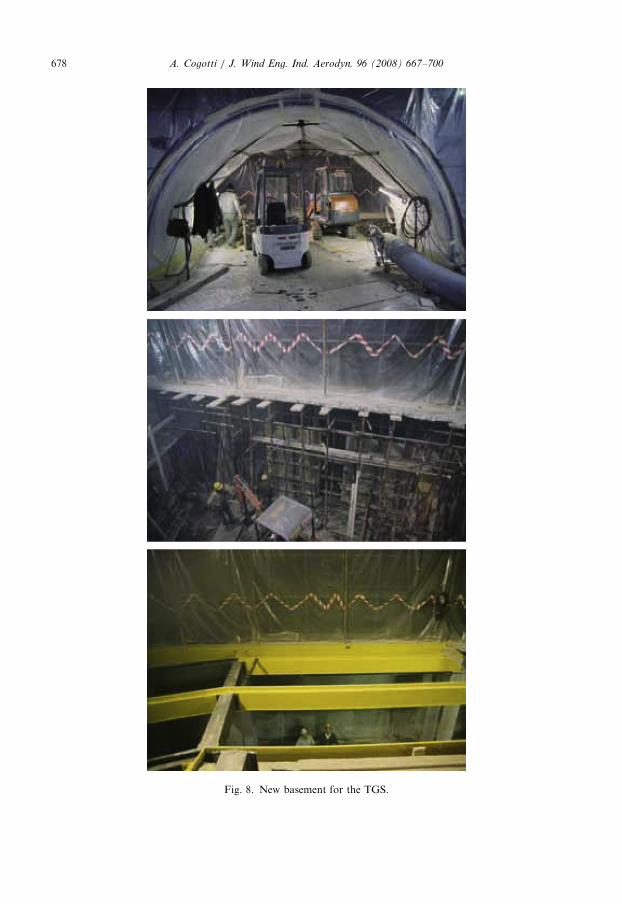

ARTICLE IN PRESS

Fig. 8. New basement for the TGS.


ARTICLE IN PRESS

Fig. 9. (a) Final prototypes of the turbulence generators.

Fig. 9. (b) some views of the final TGS in operation since January 2003.



a turbulence intensity lateral component greater than the longitudinal component, anda TLS in the order of 1m or more.Fig. 9b shows the final system, in operation since January 2003. The 5 final turbulencegenerators have flaps made of carbon fiber to achieve a higher flapping frequency (up to1Hz). They are usually parked under the nozzle. Being installed on lifters, when needed,they can be raised into the nozzle in a short time (about 103000). They can be removedand parked again, in the same short time. This way the TGS can be easily used inaddition to the standard low-turbulence tests, not instead of them, to checkaerodynamics and aeroacoustics of the new car models, when necessary, in conditionsof a turbulent flow too. Depending on the mode of operation of the 5 TGs, the flow hascharacteristics in the following range:

2.
log law of the wall velocity profile, a�0.16–0.24. 3. turbulence intensity I up to 7–8% [0.3–0.7%]. 4. Iv/Iu�1.3–1.4 5. TLS up to 1.0–2.0m [o0.1m ? ].
The values in brackets [ ] are the values of the base wind tunnel, without TGS.Possible modes of operation include:

1.
TGs static, with flaps open at different angles, from 151 to 451, mode 1. 2. TGs flapping at a constant frequency, from 0 to 1Hz, in-phase, mode 2a, or out-of-
phase, mode 2b.
3. TGs flapping at a continuously varying frequency, from a min. to a max, within periods
that vary according to various possible laws, so as to achieve a ‘pseudo-random’behavior. Again the 5 TGs can flap in-phase, mode 3a, or out-of-phase, mode 3b. Themode 3b is the one that is used at present to simulate the turbulence generated by a lightwind.

New modes of operation are under investigation as explained later.Each mode of operation generates a flow having different characteristics of velocity

distribution and turbulence. They are summarized in Table 1. Mode of operation 1( ¼ TGs static at a given angle of aperture of the flaps) can be used

�
to check the car response in the condition of low turbulence (I ¼ 3.9%, TLS ¼ 0.17m)when the angle of the flaps is kept to the minimum, or (I ¼ 5.9%, TLS ¼ 0.18m) whenthe angle of the flaps is kept to the parking position. � to check the car response in the condition of higher turbulence (I ¼ 10.2%,
TLS ¼ 0.29m) and mainly in the presence of 2 large vortices that appear in the flow,when the angle of the flaps is large (Fig. 10a). These vortices are similar to those shed bya down-lifting car, like a racing car. They induce on the car in the test section a strongfront lift. It could be used to check the behavior of a racing car in the wake of anotherracing car.

The mode of operation 2 ( ¼ 5 TGs flapping at a given frequency) can be used to checkthe car response to that specific frequency. A possible flapping frequency (0.2Hz) is easilyvisible in the PSD, see Fig. 11a.

ARTICLE IN PRESS

Table 1

Summary of the flow turbulence characteristics corresponding to the various modes of operation

TGs mode X (m) Y (m) H (m) I % Iu % Iv % Iv/Iu TLS (m)

3b-random Out of phase Bal. center 0 0.5 7.5 5.8 7.9 1.35 0.68

3b-random Out of phase Bal. center �1 0.5 6.0 5.0 6.3 1.27 0.53

3b-random Out of phase �2.5 0 0.5 8.0 5.8 8.7 1.50 0.61

3a-pseudo-random In phase Bal. center 0 0.5 7.8 5.8 7.6 1.31 1.53

2–0.2Hz In phase Bal. center 0 0.5 8.0 6.0 7.7 1.29 2.56

1 Flap angle ¼ minimum Bal. center 0 0.5 3.9 3.0 4.3 1.43 0.17

1 Flap angle ¼ lift Bal. center 0 0.5 5.9 4.7 6.7 1.42 0.18

1 Flap angle ¼ minimum Bal center 0 0.5 10.2 7.7 10.4 1.53 0.29

Fig. 10. (a) TGS setup that generates up-wash and (b) TGS setup that generates down-wash.


�
The turbulence intensity at h ¼ 0.5m, x ¼ bal. center, y ¼ 0 is I ¼ 8.0%, Iu ¼ 6.0%,Iv ¼ 7.7%, Iv/Iu ¼ 1.29. � The integral scale of the turbulence TLS ¼ 2.56m (autocorrelation method).
Mode 2 could be used, in principle, in wind engineering too, to check the response of abuilding (or a bridge, etc.) to a flow periodically varying at a constant frequency chosen inthe range 0.01–1.00Hz. Considering the size of the wind tunnel open jet (11m2) the scalemodel could have a frontal area up to 2.5–3.0m2, depending on the shape of the model.

ARTICLE IN PRESS

Fig. 11. (a) Power spectral density for the 0.2Hz flapping mode, versus the base wind tunnel.

Fig. 11. (b) Power spectral density for 2 TGS setups versus the base wind tunnel.


The mode of operation 3a ( ¼ 5 TGs in-phase) generates more turbulence and a largerTLS , see ‘setup 2’ in Fig. 11b:

�
The turbulence intensity at h ¼ 0.5m, x ¼ bal. center, y ¼ 0 is I ¼ 7.8%, Iu ¼ 5.8%,Iv ¼ 7.6%, Iv/Iu ¼ 1.31. � The integral scale of the turbulence TLS ¼ 1.53m (autocorrelation method).
The mode of operation 3b ( ¼ 5 TGs out-of-phase) that at present is considered the bestto simulate the turbulence generated by a light wind, has the following characteristics:

�
The TGs flap out of phase, at a frequency varying from 0.1 to 0.75Hz in a periodvarying from 15 to 6000. All these parameters may be easily changed by computer. � The dynamic pressure profile generated in the test section is shown in Fig. 12a. � The PSD measured at h ¼ 0.5m, x ¼ bal. center, y ¼ 0m is shown in Fig. 11b as
‘setup 1’.

ARTICLE IN PRESS

Fig. 12. (a) Dynamic pressure distribution at the balance center-mode 3b.

Fig. 12. (b) Noise inside a car due to the TGS.


�
The turbulence intensity: I ¼ 7.5%, Iu ¼ 5.8%, Iv ¼ 7.9%, Iv/Iu ¼ 1.35. � The integral scale of the turbulence is TLS ¼ 0.68m (autocorrelation method).
The time-averaged flow is reasonably uniform both as velocity distribution in X and Y aswell as turbulence intensities.

In fact, at h ¼ 0.5m, x ¼ bal. center, y ¼ �1m:

�
The turbulence intensity: I ¼ 6.0%, Iu ¼ 5.0%, Iv ¼ 6.3%, Iv/Iu ¼ 1.27. � The integral scale of the turbulence TLS ¼ 0.53m (autocorrelation method).
At h ¼ 0.5m, x ¼ �2.5m from the bal. center, y ¼ 0m,

�
The turbulence intensity I ¼ 8.0%, Iu ¼ 5.8%, Iv ¼ 8.7%, Iv/Iu ¼ 1.50. � The integral scale of the turbulence TLS ¼ 0.61m (autocorrelation method).
From a subjective stand point, mode 3b is one of the preferred as, beside anyconsideration regarding the PSD or the TLS, it gives an acoustic subjective feeling, that,


according to some people, recalls, better than other modes, the noise that is heard by thedriver when a car is moving on the road.It is worth noticing that the noise generated by the flapping of the 5 TGs is much lower

than the ambient noise in the test section. Fig. 12b shows the noise measured inside a car,with the TGs flapping, in the 2 conditions of ‘no wind’ and wind at 140 km/h. Thereforethe TGS noise does not affect at all the aeroacoustic measurements on the vehicles.In conclusion the TGS offers the possibility of testing in a number of turbulent flows.

Each of them can be easily generated by changing by computer the mode of operation.Other possible modes of operation are in course of investigation. In particular it has beenshown already the possibility of simulating the following flows:

�
A flow that simulates the presence of another car upstream the car in the test section: Thisflow induces a change in the front lift of the car that follows. That change can be easilymeasured and linked to the vorticity or to the local flow angle of the approaching flow.See examples in Figs. 10a and b. � An oscillating flow that induces a dynamic yaw on the car.
This work is in progress, it will be reported in a future paper.

2.4. Some examples of results with the TGS

2.4.1. Aerodynamics

This paragraph reports examples of measurements made in different test conditions:

1.
Base wind tunnel, i.e., say a low-turbulence flow and a flow velocity corresponding tothe car velocity (conventional test condition).
2.
Wind tunnel+turbulence generation system, at Vwt ¼ Vcar, i.e., turbulent flow and flowvelocity corresponding to the car velocity (to check the effect of the increased turbulenceonly).
3.
Wind tunnel+turbulence generation system, at Vwt4Vcar, i.e., turbulent flow and flowvelocity corresponding to the car velocity+the ambient wind velocity. This condition isthat similar to the actual road condition. It shows the combined effect of the increasedturbulence and of the increased resultant wind velocity, while the moving groundvelocity is kept constant.
2.4.1.1. Force measurements, time-averaged values. The following diagrams show anexample of time-averaged values measured on a car in the 3 different testing conditions(Fig. 13).The CD diagram shows a small increase of drag due to the increased turbulence, and a

larger increase when the wind tunnel velocity is increased to account for the presence ofambient wind. In this last case the CD values are referred to the moving ground velocity.The front lift CLF shows a similar trend. However, the effect of the turbulence (and of

the velocity profile) is, in this case, more important.Fig. 14 shows results (CD and CLF) measured on a second car (wagon type), in the first

and second test conditions. The trend is the same, increase of CD and CLF with theturbulence. Furthermore, the vertical bars show the fluctuation (Std. Dev.) of thesecoefficients in the time. This fluctuation is quite large for the front lift.

ARTICLE IN PRESS

Fig. 13. CD and CLF mean values measured at different yaw angles and in 3 different test conditions.

Drag Coefficient Car W - Wagon

0.320.330.340.350.360.370.380.390.40

-5

Yaw Angle [ ° ]

CD

TGS ON

TGS Off

Front Lift Car W - Wagon

-0.10

-0.05

0.00

0.05

0.10

CLFTGS ON

TGS Off

Yaw Angle [ ° ]

151050-5 151050

Fig. 14. CD and CLF mean values and standard deviation, in 2 different test conditions.


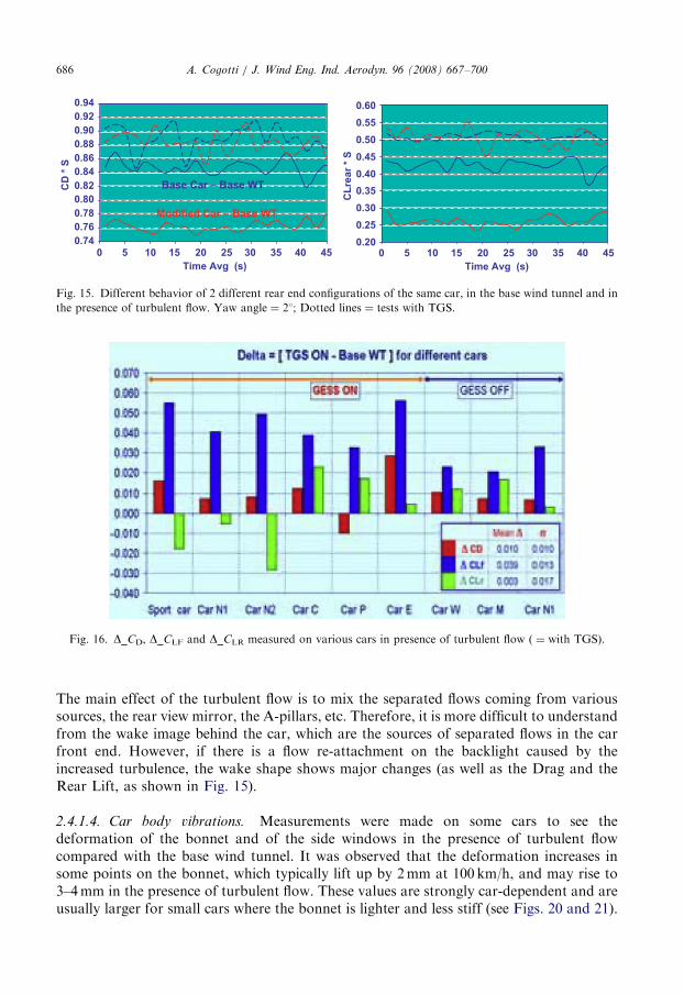
The rear lift mean value CLR usually does not change too much. However, it may show alarge increase in some cars, having a rounded upper edge over the backlight. The wake ofthese cars is critical. An increase of turbulence in approaching flow may reattach the flowon the backlight, causing a noticeable increase of drag and rear lift, Fig. 15.

Different cars show different behaviors. Although the number of tests made up to thetime of the writing of this paper, is not very large, some statistics can be made and theresults can be seen in Fig. 16.

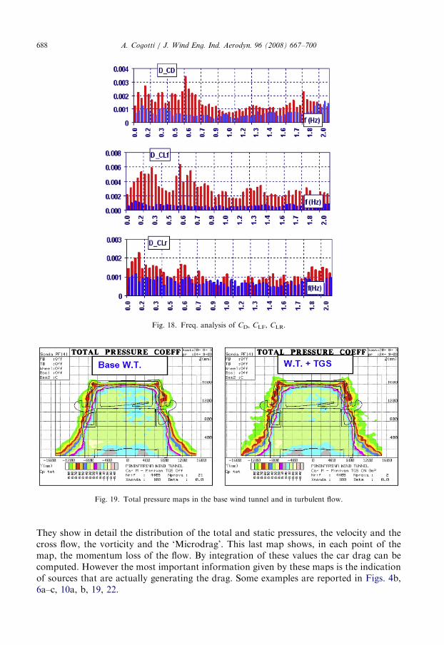
2.4.1.2. Force measurements, time-dependent values. Figs. 17 and 18 show the timehistory and the frequency spectrum of the fluctuating part of the 3 coefficients, CD, CLF,CLR. These values are filtered 2Hz low pass. It can be seen that, in general, the fluctuationin time of the coefficients increases in the presence of turbulent flow. As a consequence, toget repeatable mean values a longer integration time (typically 12000) is necessary.

Sometime, there might be a re-attachment of the flow on the backlight, due to theincreased turbulence and, therefore, the rear lift coefficient (CLR) increases both as meanvalue (Fig. 15) and as fluctuation.

2.4.1.3. Flow field maps, time-averaged values. Fig. 19 shows the total pressure mapmeasured behind a minivan in the base wind tunnel and in turbulent flow condition.

ARTICLE IN PRESS

Fig. 16. D_CD, D_CLF and D_CLR measured on various cars in presence of turbulent flow ( ¼ with TGS).

0.200.250.300.350.400.450.500.550.60

0 5 10 15 20 25 30 35 40 45Time Avg (s)

0 5 10 15 20 25 30 35 40 45Time Avg (s)

CLr

ear *

S

0.740.760.780.800.820.840.860.880.900.920.94

CD

* S

Base Car – Base WT

Modified Car – Base WT

Fig. 15. Different behavior of 2 different rear end configurations of the same car, in the base wind tunnel and in

the presence of turbulent flow. Yaw angle ¼ 21; Dotted lines ¼ tests with TGS.


The main effect of the turbulent flow is to mix the separated flows coming from varioussources, the rear view mirror, the A-pillars, etc. Therefore, it is more difficult to understandfrom the wake image behind the car, which are the sources of separated flows in the carfront end. However, if there is a flow re-attachment on the backlight caused by theincreased turbulence, the wake shape shows major changes (as well as the Drag and theRear Lift, as shown in Fig. 15).

2.4.1.4. Car body vibrations. Measurements were made on some cars to see thedeformation of the bonnet and of the side windows in the presence of turbulent flowcompared with the base wind tunnel. It was observed that the deformation increases insome points on the bonnet, which typically lift up by 2mm at 100 km/h, and may rise to3–4mm in the presence of turbulent flow. These values are strongly car-dependent and areusually larger for small cars where the bonnet is lighter and less stiff (see Figs. 20 and 21).

ARTICLE IN PRESS

Fig. 17. Example of time history of CD, CLF, CL.


3. Measuring techniques

In order to understand the details of the flow field and decide what to do during the cardevelopment it is important to improve the existing measuring techniques. In thefollowing, a short description is given of some of the main measuring techniques set up inPininfarina (Cogotti, 1998b, c, 2000, 2003d) and used at present to speed up thedevelopment work.

3.1. Pressure probe to survey the flow around the car

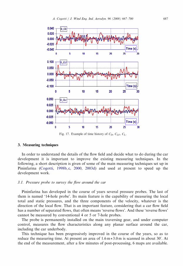
Pininfarina has developed in the course of years several pressure probes. The last ofthem is named ‘14-hole probe’. Its main feature is the capability of measuring the localtotal and static pressures, and the three components of the velocity, whatever is thedirection of the local flow. That is an important feature, considering that a car flow fieldhas a number of separated flows, that often means ‘reverse flows’. And these ‘reverse flows’cannot be measured by conventional 4 or 5 or 7-hole probes.

The probe is permanently installed on the main traversing gear, and under computercontrol, measures the flow characteristics along any planar surface around the car,including the car underbody.

This technique has been progressively improved in the course of the years, so as toreduce the measuring time. At present an area of 1.6m*3.0m is scanned in about 300. Atthe end of the measurement, after a few minutes of post-processing, 6 maps are available.

ARTICLE IN PRESS

Fig. 18. Freq. analysis of CD, CLF, CLR.

Fig. 19. Total pressure maps in the base wind tunnel and in turbulent flow.


They show in detail the distribution of the total and static pressures, the velocity and thecross flow, the vorticity and the ‘Microdrag’. This last map shows, in each point of themap, the momentum loss of the flow. By integration of these values the car drag can becomputed. However the most important information given by these maps is the indicationof sources that are actually generating the drag. Some examples are reported in Figs. 4b,6a–c, 10a, b, 19, 22.

ARTICLE IN PRESS

Figs. 20,21. Time history of the bonnet vibration in the base wind tunnel and in conditions of turbulent flow.

Fig. 22. Flow interference between cooling towers—scale 1:100. The wake of the upstream tower produces an

asymmetric suction on the sides of the downstream tower.


This technique has been used in the past also in the course of some wind engineeringtests that, time and again, are carried out in our wind tunnel. In the case shown in Fig. 22,it was requested to measure the flow field around a cooling tower, located downstreamanother cooling tower. These flow interference effects are important. A simple flowvisualization by smoke and laser light sheet was not sufficient, it was important in this caseto get quantitative information about pressures and velocities.

3.2. Laser doppler velocimetry

A special fiber-link 3-D LDV system is available in the wind tunnel to measure velocities(3 comp.) and turbulence, with no physical interference with the flow. Main features are:

�
miniature end probe, Fig. 23a, � fiber-optic link,

ARTICLE IN PRESS

Fig. 23. (a) Laser generator and main optics miniature end-probe.

Fig. 23. (b) Histograms of the 3 vel. components in a point of a matrix behind the rotating wheel.


�
high accuracy, � high spatial resolution (meas. volume of 0.5m*1.5mm), � time-resolved measurements.
It is mainly used for measurements:

�
close to the car surface, in the boundary layer, � close to rotating parts (radiator fans, wheels, see Fig. 23b) or inside the rotating wheel
disk openings to measure the disk cooling flow,
� within the engine bay, where the flow is more difficult to measure, being low velocity
and time dependent both as magnitude and direction (Cogotti and Berneburg, 1991;Berneburg and Cogotti, 1993; Cogotti and De Gregorio, 2000).

ARTICLE IN PRESSA. Cogotti / J. Wind Eng. Ind. Aerodyn. 96 (2008) 667–700 691

And these measurements are often used to validate CFD simulations or PIVmeasurements.

3.3. Recirculation of exhaust gases and backlight soiling

Fig. 24 shows an example of recirculation of exhaust gases. The image is taken atY ¼ exhaust pipe.

Fig. 25 shows an example of backlight soiling. The image is taken at Y ¼ 0 ¼ center line.Both are examples of unsteady flows at the car rear end.

The visualization is made by the help of smoke and a laser light sheet.In both cases, tests are made with moving ground and rotating wheels. This last point is

important to correctly reproduce the behavior of the exhaust gases and of the soiling.

3.4. PIV

The ‘particle image velocimetry’ or PIV is a recent technique that is capable of providingquantitative velocity information, instantaneously, at a large number of points.

This feature gives the possibility to identify the flow structures and, to some extent, theirevolution in the time.

PIV system of various types are already successfully in operation in many wind tunnel(mainly of small size) and in water tunnels, for instance at INSEAN in Italy (Calcagno etal., 2004; Albano and De Gregorio, 2004).

A Stereo-PIV system is at present in course of development at Pininfarina. Althoughthe technique itself is pretty well known, its application in a full-scale automotivewind tunnel presents a number of technical and practical problems that are not yetcompletely fixed.

Fig. 24. Recirculation of exhaust gases.

ARTICLE IN PRESS

Fig. 25. Backlight soiling. Visualization by laser light-sheet and smoke on laser light-sheet and smoke on the car

centerline.


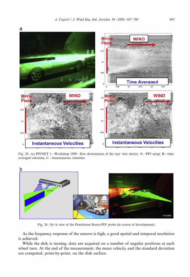
The first of this problem is the setup time. It is usually quite long, not acceptable in anautomotive wind tunnel, where the available time is always limited.The PIV probe in course of development at Pininfarina (Fig. 26b) intends to optimize

the setup time, improve the optical access and in general to make this technique easy to usein the every day work.Some examples of PIV measurements made in the past are shown in Fig. 26a, and those

recently made in Fig. 26c.As one can understand from these images, the technique is quite powerful, and it is

probably the best technique to be used in the future to investigate unsteady flows.

3.5. Disk brake cooling

A limitation that is peculiar is the tests in the purely aerodynamic wind tunnel is theimpossibility of measuring the real cooling of the brake disks. Often modifications made tothe car front end to reduce the CD reduce the brake cooling and that can be checked onlywhen the same car configuration is re-tested in a climatic wind tunnel.In order to fix this problem a technique has been developed recently in Pininfarina. This

technique uses some sensors embedded on the brake disk, to measure the tangentialvelocity on the disk while the wheels are rotating.The sensors are applied on each side of the disk, so that the cooling effect can be

measured on the inner and outer sides of the disk.The sensors are ‘hot-film’ type, conveniently modified in house so as to be applicable on

the disk surface. They are calibrated in terms of tangential velocity. However what theyactually measure is the heat exchange between the rotating disk and the surrounding flow.

ARTICLE IN PRESS

Fig. 26. (a) PIVNET 1—Workshop 1999—flow downstream of the rear view mirror. A—PIV setup, B—time-

averaged velocities, C—instantaneous velocities.

Fig. 26. (b) A view of the Pininfarina Stereo-PIV probe (in course of development).


As the frequency response of the sensors is high, a good spatial and temporal resolutionis achieved.

While the disk is turning, data are acquired on a number of angular positions at eachwheel turn. At the end of the measurement, the mean velocity and the standard deviationare computed, point-by-point, on the disk surface.

ARTICLE IN PRESS

Fig. 26. (c) Example of PIV measure at the car side through the open window at Z ¼ 1100 and 1200mm.

Fig. 27. (a) Sensors on the brake disk for cooling measurement.


Fig. 27a shows the sensors applied on the brake disk.Fig. 27b shows an example of results measured on 2 different car configurations, with

and without a dam on the front bumper. In particular, it can be seen that

�
the dam reduces the disk cooling, � the cooling effect is larger on the disk inner side than on the outer side, � the cooling efficiency reduces at high speed, i.e. when the wind velocity is increased.
Some discontinuity in the trend suggests the existence of local flow separations that arevelocity and/or turbulence dependent.

ARTICLE IN PRESS

Fig. 27. (b) Velocity distribution on the inner and outer sides of the brake disk.


3.6. Sunroof booming

Sunroof booming is a very common feature of many cars when the sunroof is fully open.It typically happens at low velocity and the booming peak has a low frequency in the orderof 20Hz.

Fig. 28a shows an example of noise spectra measured by an acoustic head with thesunroof open. The booming peak is clearly visible. Fig. 28b shows a visualization of theshear layer over the sunroof opening. It is an unsteady flow typical of passenger car.

The oscillation of the shear layer is the source of the booming and it can be affected bythe turbulence of the incoming flows.

3.7. Buffeting on open roof cars

Another typical problem of open roof cars is the flow buffeting around the heads of thepassengers. The buffeting is usually reduced with the help of some flaps on the windscreenupper frame or by wind stoppers at the rear of the passenger heads.

A practical way to obtain a quantitative indication of this buffeting is the measure of thelocal velocity fluctuation on the head of a dummy. This is made in Pininfarina by using ahelmet (named ‘comfort helmet’) equipped with a number of sensors. These sensorsmeasure the local velocity as well as the fluctuation of the velocity. Again the mean velocityin each point and its fluctuating part may depend on the level of turbulence intensity of theflow approaching the car. Fig. 29a shows an example of the test setup. Fig. 29b shows anexample of results measured in the condition of low-turbulence (left image) and high-turbulence flow (right image).

ARTICLE IN PRESS

Fig. 28. (a). Frequency spectrum of the sunroof booming.

Fig. 28. (b) Visualization of the flapping shear booming layer over the sunroof open cavity.


3.8. Soft top deformation

The deformation of the soft top caused by the aerodynamic loading is another featurethat has to be kept under control by a suitable measurement technique. The amount ofdeformation cannot exceed a given value for esthetic reasons and to avoid noise infiltrationthrough the soft tops sealing.The technique used in Pininfarina uses a small laser that moves along the soft top

centerline , and measures the soft top profile, at first without wind, and then with the windat one or more velocity. The difference of profile gives an accurate indication of the softtop deformation. An example is shown in Fig. 30.The same technique is used to measure the deformation of side glasses, mainly at yaw, or

of other mobile parts under aerodynamic load.

ARTICLE IN PRESS

Fig. 29. (a) ‘Comfort Helmet’ on the head of the acoustic dummy.

Fig. 29. (b) Mean vel. and std. dev. on each point of the helmet, in the base WT (left) and with the turbulence

generators (right).

0200400600800

1000120014001600

-400 100 600

H (m

m)

0

20

40

60

80

100

Delta

H (m

m)

Profilo Capote a V=0Profilo Capote a V=120 km/hDelta H (mm)

1100

Fig. 30. Measure of the deformation of the soft top under aerodynamic loading.



4. Wind engineering

The Pininfarina wind tunnel works mainly in the automotive field. However, timeby time, we are asked to perform aerodynamic or aeroacoustic tests in other fields, from

Fig. 31. Examples of non-automotive tests (aerodynamic or aeroacoustic), carried out on various types of: trains

(1:7.5), cooling towers (1:100), buildings-bridges-wind barriers, in large scale, with or without turbulent flow.

ARTICLE IN PRESSA. Cogotti / J. Wind Eng. Ind. Aerodyn. 96 (2008) 667–700 699

high-speed trains to buildings of various type that belong to the wind engineering field.That is because of the size of the wind tunnel open jet (larger than the most of the windengineering wind tunnels), or of the requested top speed, or of the measuring techniquesthat are necessary for some tests and that are not available in other wind tunnels. Someexample of these tests are shown in Fig. 31.

5. Conclusion

The continuous evolution of the road vehicles demands a parallel continuous evolutionof the facilities and of the measuring techniques, so as to be able to face the newrequirements. Obviously the same happens in a number of other fields. All that requirescontinuous investments to upgrade the facilities and the measuring techniques. Pininfarinahas a firm commitment to accept this challenge. At present a new important upgrading ofthe wind tunnel is in progress. The aim is to increase the top speed to about 250 km/h and,at the same time, to further reduce the ambient noise in the test section by about 5 dB. Theend of this work is planned to finish around mid 2005.

References

Albano, F., De Gregorio, F., 2004. Large aircraft wake vortex characterisation at insean towing tank. Pivnet 2. In:

Workshop on Applications of PIV to Naval and Industrial Hydrodynamics. INSEAN, Rome 5 May 2004.

Berneburg, H., Cogotti, A., 1993. Development and use of ldv and other airflow measurement techniques as a

basis for the improvement of numerical simulation of engine compartment air flows. In: SAE Paper 930294,

International SAE Congress, Detroit, February 1993.

Calcagno, G., Pereira, F., Felli, M., Di Felice, F., 2004. A stereo PIV underwater probe for towing tank

applications. In: Pivnet 2, Workshop on Applications of PIV to Naval and Industrial Hydrodynamics,

INSEAN, Rome 5 May 2004.

Cogotti, A., 1995. Ground effect simulation for full-scale cars in the Pininfarina wind tunnel. In: SAE Paper

950996, International SAE Congress, Detroit, February–March 1995.

Cogotti, A., 1997. Aeroacoustics development in Pininfarina. In: SAE paper 970402, International SAE Congress,

Detroit, February 1997.

Cogotti, A., 1998a. A parametric study on the ground effect of a simplified car model. In: SAE Paper no. 980031,

International SAE Congress, Detroit, February 1998.

Cogotti, A., 1998b. Flow visualization techniques in the Pininfarina full-scale automotive wind tunnel. In: Eighth

International Symposium on Flow Visualization, Sorrento, Italy, September 1998.

Cogotti, A., 1998c. Measurement techniques in vehicle aerodynamics. Euromotor International Short Course on

Vehicle Aerodynamics, Stuttgart, February 1998.

Cogotti, A., 1999. Ground effect of a simplified car model in side-wind and turbulent flow. In: SAE Paper no.

1999-01-0652, International SAE Congress, Detroit, March 1999.

Cogotti, A., 2000. Flow field measurements and their interpretation. Euromotor International Short Course on

Vehicle Aerodynamics, Stuttgart, February 2000.

Cogotti, A., 2001. Flow field of an isolated rotating wheel. Preliminary results. ECARA–Ground Simulation

Committee, FKFS, Stuttgart, 10 October, ppt presentation only.

Cogotti, A., 2002. Preliminary information about unsteady aerodynamics techniques at Pininfarina. ECARA

Unsteady Aerodynamics Committee—Fourth Meeting, Torino, October 2002.

Cogotti, A., 2003a. Generation of a controlled level of turbulence in the Pininfarina wind tunnel for the

measurement of unsteady aerodynamics and aeroacoustics. In: SAE 2003-01-0430, International SAE

Congress, March 2003.

Cogotti, A., 2003b. Unsteady aerodynamics at Pininfarina. road turbulence simulation and time-dependent

techniques. In: Fifth International Stuttgart Symposium, February 2003.

Cogotti, A., 2003c. Additional information on the Pininfarina turbulence generation system. ECARA Unsteady

Aerodynamics Committee—Fifth Meeting, Munich, April 2003.


Cogotti, A., 2003d. From steady-state to unsteady aerodynamics and aeroacoustics. The evolution of the testing

environment in the Pininfarina wind tunnel. In: Seventh International Symposium on Fluid Control,

Measurement and Vision, Sorrento, August 2003.

Cogotti, A., 2004. Update on the Pininfarina turbulence generation system and its effects on the car aerodynamics

and aeroacoustics. In: SAE Paper no. 2004-01-0807, International SAE Congress, Detroit, March 2004.

Cogotti, A., Berneburg, H., 1991. Engine compartment airflow investigations using a laser-doppler-velocimeter.

In: SAE Paper 910308, International SAE Congress, Detroit, February 1991.

Cogotti, A., De Gregorio, F., 2000. Presentation of flow field investigation by piv on a full-scale car in the

Pininfarina wind tunnel. In: SAE 00B-112, International SAE Congress, Detroit, March 2000.

Cooper, K.R., 1989. The wind tunnel simulation of wind turbulence for surface vehicle testing. In: Eighth

Colloquium on Industrial Aerodynamics, Aachen, September 4–7, 1989.

Cooper, K.R., 1991. Wind tunnel simulation of wind turbulence for surface vehicle testing. J. Wind Eng. Ind.

Aerodyn. 38, 71–81.

Gilhome, B.G., Saunders, J.W., 2002. The effect of turbulence on peak and average pressures on a car door. SAE

2002-01-0253.

Gilhome, B.G., Saunders, J.W., Sheridan, J., 2001. Time averaged and unsteady near-wake analysis of cars. SAE

2001-01-1040.

Howell, J., 2000. Real environment for vehicles on the road. In: Euromotor 2000. FKFS, Stuttgart.

Macklin, A.R., Garry, K.P., Howell, J.P., 1997. Assessing the effects of shear and turbulence during the dynamic

testing of the crosswind sensitivity of road vehicles. SAE 970135.

Saunders, J.W., Mansour, R.B., 2000. On-road and wind tunnel turbulence and its measurements using a four-

hole dynamic probe ahead of several cars. SAE 2000-01-0350.

Saunders, J.W., Watkins, S., 1993. Atmospheric effects on the crosswind stability of cars. In: Goetz, H. (Ed.),

Contribution to the American SAE Information Monograph of the Crosswind Stability of Cars, SAE SP-

1109.

Saunders, J.W., Watkins, S., Hoffmann, P.H., Buckley Jr., F.T., 1985. Comparison of on-road and wind-tunnel

tests for tractor-trailer aerodynamic devices, and fuel savings predictions. SAE Paper 850286, SAE Congress,

Detroit, February 1985, subsequently published in 1985 SAE Transactions.

Szechenyi, E., 2000. Crosswind and its simulation. In: Euromotor 2000. FKFS, Stuttgart.

Vernacchia, M., 1990. Medium class vehicle with high aerodynamic efficiency. FISITA Paper 905127, Torino,

May 1990.

Watkins, S., Saunders, J.W., 1995. Turbulence experience by road vehicles under normal driving conditions. SAE

Paper 950997, 1995.

Watkins, S., Saunders, J.W., 1998. A review of the wind conditions experienced by a moving vehicle. SAE Paper

981182, 1998.

Watkins, S., Toksoy, S., Saunders, J.W., 1992. On the generation of tunnel turbulence for road vehicles. In:

Eleventh Australasian Fluid Mechanics Conference, University of Tasmania, Hobart, Australia, 14–18

December 1992.

Further reading

Cogotti, A., Cardano, D., Carlino, G., Cogotti, F., 2005. Aerodynamics and aeroacoustics of passenger cars in a

controlled high turbulence flow: Some new results. SAE paper no 2005-01-1455.

Cogotti, A., 2006. Upgrade of the Pininfarina wind tunnel—The new ‘‘13-fan’’ drive system. SAE paper 2006-01-

0569.

Cogotti, A., 2007. The new moving ground system of the Pininfarina wind tunnel. SAE paper 2007-01-1044.

Lindener, N., Miehling, H., Cogotti, A., Cogotti, F., Maffei, M., 2007. Aeroacoustic measurements in turbulent

flow on the road and in the wind tunnel. SAE paper 2007-01-1551.

Evolution of performance of an automotive wind tunnel · PDF fileEvolution of performance of...

Documents

Transcript of Evolution of performance of an automotive wind tunnel · PDF fileEvolution of performance of...