Competition’s effect on productivity: Treatment or selection?

1

Evidence from BLADE

Robert Tiong11/10/2019

University of New South WalesSupervisors: Prof. Kevin Fox

Dr Shengyu Li

1. How has market competition been growing over time?

- HHI, mean and median size of firms: Grullon, Larkin and Michaely (2018)

- Markups: De Loecker and Eeckhout (2017); Edmonds et al. (2019)

2. Does changes in competition contribute to firm-level productivity?

3. Can markets benefit from institutional changes to competition in Australia, and if so, how?

Research Questions

2

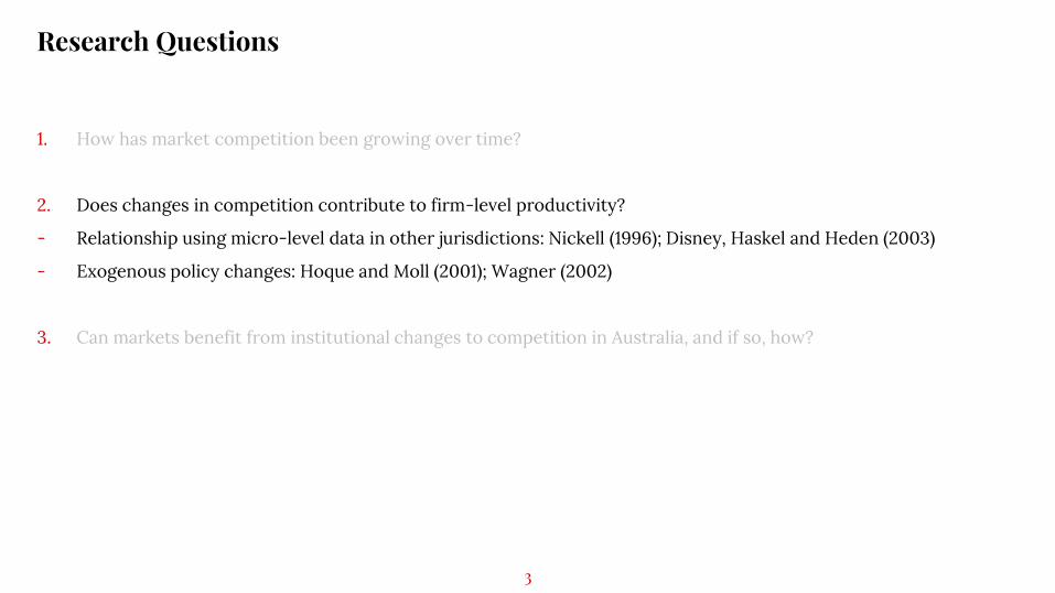
1. How has market competition been growing over time?

2. Does changes in competition contribute to firm-level productivity?

- Relationship using micro-level data in other jurisdictions: Nickell (1996); Disney, Haskel and Heden (2003)

- Exogenous policy changes: Hoque and Moll (2001); Wagner (2002)

3. Can markets benefit from institutional changes to competition in Australia, and if so, how?

Research Questions

3

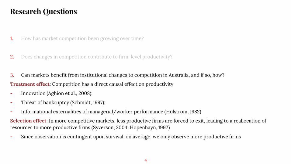
1. How has market competition been growing over time?

2. Does changes in competition contribute to firm-level productivity?

3. Can markets benefit from institutional changes to competition in Australia, and if so, how?

Treatment effect: Competition has a direct causal effect on productivity

- Innovation (Aghion et al., 2008);

- Threat of bankruptcy (Schmidt, 1997);

- Informational externalities of managerial/worker performance (Holstrom, 1982)

Selection effect: In more competitive markets, less productive firms are forced to exit, leading to a reallocation of resources to more productive firms (Syverson, 2004; Hopenhayn, 1992)

- Since observation is contingent upon survival, on average, we only observe more productive firms

Research Questions

4

New firm-level data of all active businesses from 2001-02 to 2015-16

I estimate:

- Productivity: Wooldridge (2009); Diewert and Fox (2010)

- Olley and Pakes; Levinsohn and Petrin; Labour Productivity

- Competition: Herfindahl-Hirschmann Index; Change in Market Share

- Markups; Concentration Ratios

Business Longitudinal Analysis Data Environment (BLADE)

5

Government Administrative Data

Business Activity Statements

Business Income Tax Filings

Pay As You Go Summaries

ABS Survey Data

Business Characteristics Survey

Economic Activity Survey

Business Expenditure on Research and Development

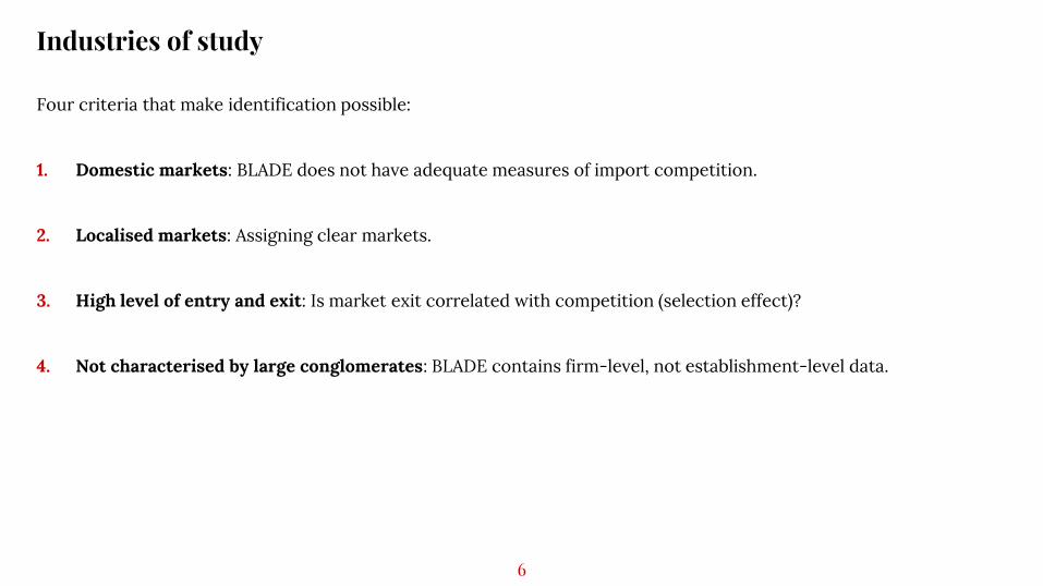
Four criteria that make identification possible:

1. Domestic markets: BLADE does not have adequate measures of import competition.

2. Localised markets: Assigning clear markets.

3. High level of entry and exit: Is market exit correlated with competition (selection effect)?

4. Not characterised by large conglomerates: BLADE contains firm-level, not establishment-level data.

Industries of study

6

Four criteria that make identification possible:

1. Domestic markets

2. Localised markets

3. High level of entry and exit

4. Not characterised by large conglomerates

- Retail Trade

- Accommodation and Food Services

Industries of study

7

Policy relevance: Two of the highest employing divisions in Australia

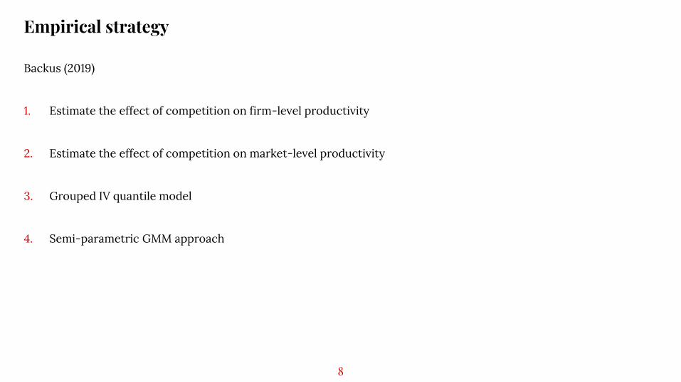
Backus (2019)

1. Estimate the effect of competition on firm-level productivity

2. Estimate the effect of competition on market-level productivity

3. Grouped IV quantile model

4. Semi-parametric GMM approach

Empirical strategy

8

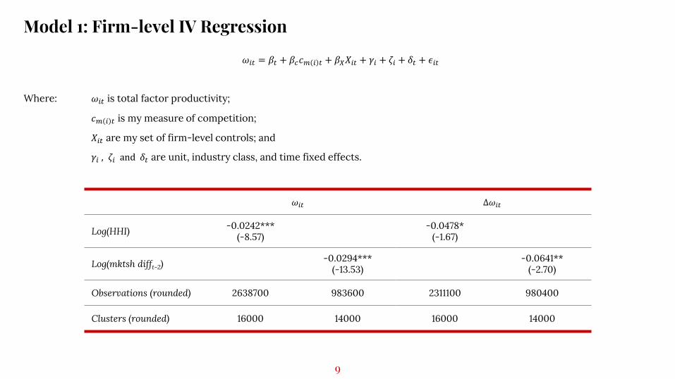
𝜔𝑖𝑡 = 𝛽𝑡 + 𝛽𝑐𝑐𝑚 𝑖 𝑡 + 𝛽𝑋𝑋𝑖𝑡 + 𝛾𝑖 + 𝜁𝑖 + 𝛿𝑡 + 𝜖𝑖𝑡

Where: 𝜔𝑖𝑡 is total factor productivity;

𝑐𝑚 𝑖 𝑡 is my measure of competition;

𝑋𝑖𝑡 are my set of firm-level controls; and

𝛾𝑖 , 𝜁𝑖 and 𝛿𝑡 are unit, industry class, and time fixed effects.

Model 1: Firm-level IV Regression

9

𝜔𝑖𝑡 Δ𝜔𝑖𝑡

Log(HHI) -0.0242***(-8.57)

-0.0478*(-1.67)

Log(mktsh difft-2)-0.0294***

(-13.53)-0.0641**

(-2.70)

Observations (rounded) 2638700 983600 2311100 980400

Clusters (rounded) 16000 14000 16000 14000

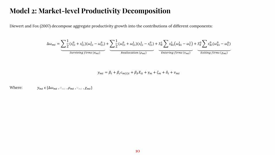
Diewert and Fox (2007) decompose aggregate productivity growth into the contributions of different components:

Δ𝜔𝑚𝑡 = 1

2(𝑠𝐶𝑖

0 + 𝑠𝐶𝑖1 )(𝜔𝐶𝑖

1 − 𝜔𝐶𝑖0 ) +

𝑆𝑢𝑟𝑣𝑖𝑣𝑖𝑛𝑔 𝑓𝑖𝑟𝑚𝑠 (𝜎𝑚𝑡)

1

2(𝜔𝐶𝑖

0 + 𝜔𝐶𝑖1 )(𝑠𝐶𝑖

1 − 𝑠𝐶𝑖0 ) +

𝑅𝑒𝑎𝑙𝑙𝑜𝑐𝑎𝑡𝑖𝑜𝑛 𝜌𝑚𝑡

𝑆𝑁1 𝑠𝑁𝑖

1 𝜔𝑁𝑖1 − 𝜔𝐶

1

𝐸𝑛𝑡𝑒𝑟𝑖𝑛𝑔 𝑓𝑖𝑟𝑚𝑠 𝜈𝑚𝑡

+ 𝑆𝑋0𝑠𝑋𝑖

0 (𝜔𝑋𝑖0 − 𝜔𝐶

0)

𝐸𝑥𝑖𝑡𝑖𝑛𝑔 𝑓𝑖𝑟𝑚𝑠 𝜒𝑚𝑡

𝑦𝑚𝑡 = 𝛽𝑡 + 𝛽𝑐𝑐𝑚 𝑖 𝑡 + 𝛽𝑋𝑋𝑖𝑡 + 𝛾𝑚 + 𝜁𝑚 + 𝛿𝑡 + 𝑣𝑚𝑡

Where: 𝑦𝑚𝑡 ϵ {Δ𝜔𝑚𝑡 , 𝜎𝑚𝑡 , 𝜌𝑚𝑡 , 𝜈𝑚𝑡 , 𝜒𝑚𝑡}

Model 2: Market-level Productivity Decomposition

10

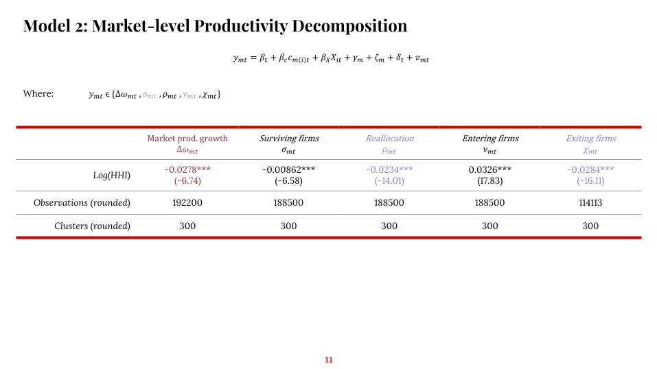
𝑦𝑚𝑡 = 𝛽𝑡 + 𝛽𝑐𝑐𝑚 𝑖 𝑡 + 𝛽𝑋𝑋𝑖𝑡 + 𝛾𝑚 + 𝜁𝑚 + 𝛿𝑡 + 𝑣𝑚𝑡

Where: 𝑦𝑚𝑡 ϵ {Δ𝜔𝑚𝑡 , 𝜎𝑚𝑡 , 𝜌𝑚𝑡 , 𝜈𝑚𝑡 , 𝜒𝑚𝑡}

Model 2: Market-level Productivity Decomposition

11

Market prod. growthΔ𝜔𝑚𝑡

Surviving firms𝜎𝑚𝑡

Reallocation𝜌𝑚𝑡

Entering firms𝜈𝑚𝑡

Exiting firms𝜒𝑚𝑡

Log(HHI) -0.0278***(-6.74)

-0.00862***(-6.58)

-0.0234***(-14.01)

0.0326***(17.83)

-0.0284***(-16.11)

Observations (rounded) 192200 188500 188500 188500 114113

Clusters (rounded) 300 300 300 300 300

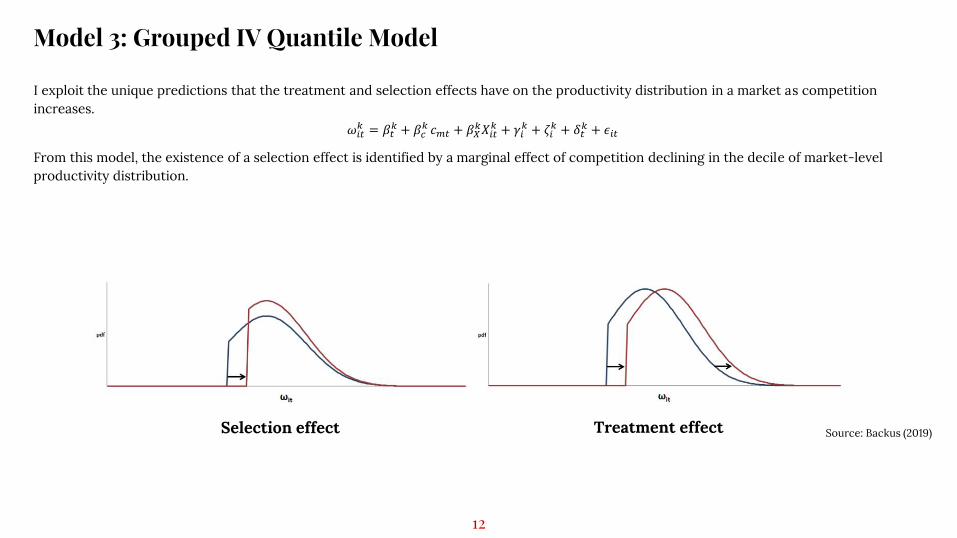
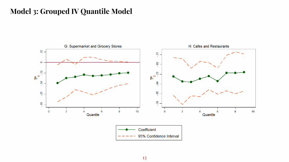
I exploit the unique predictions that the treatment and selection effects have on the productivity distribution in a market as competition increases.

𝜔𝑖𝑡𝑘 = 𝛽𝑡

𝑘 + 𝛽𝑐(𝑘 𝑐𝑚𝑡 + 𝛽𝑋

𝑘𝑋𝑖𝑡𝑘 + 𝛾𝑖

𝑘 + 𝜁𝑖𝑘 + 𝛿𝑡

𝑘 + 𝜖𝑖𝑡

From this model, the existence of a selection effect is identified by a marginal effect of competition declining in the decile of market-level productivity distribution.

Source: Backus (2019)

Model 3: Grouped IV Quantile Model

12

Selection effect Treatment effect

Model 3: Grouped IV Quantile Model

13

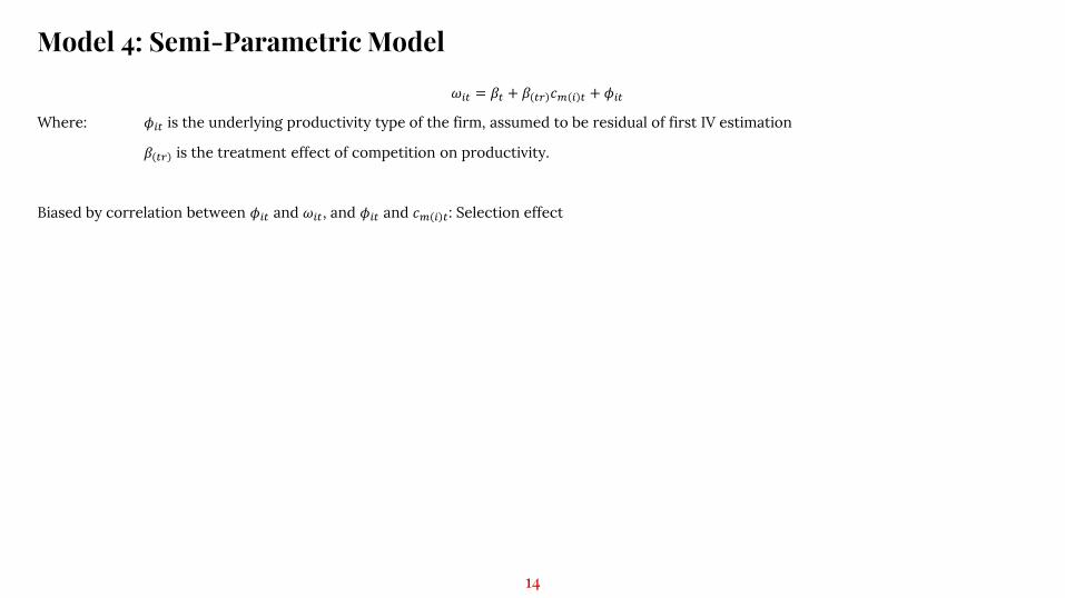
𝜔𝑖𝑡 = 𝛽𝑡 + 𝛽 𝑡𝑟 𝑐𝑚 𝑖 𝑡 + 𝜙𝑖𝑡

Where: 𝜙𝑖𝑡 is the underlying productivity type of the firm, assumed to be residual of first IV estimation

𝛽 𝑡𝑟 is the treatment effect of competition on productivity.

Biased by correlation between 𝜙𝑖𝑡 and 𝜔𝑖𝑡, and 𝜙𝑖𝑡 and 𝑐𝑚 𝑖 𝑡: Selection effect

Model 4: Semi-Parametric Model

14

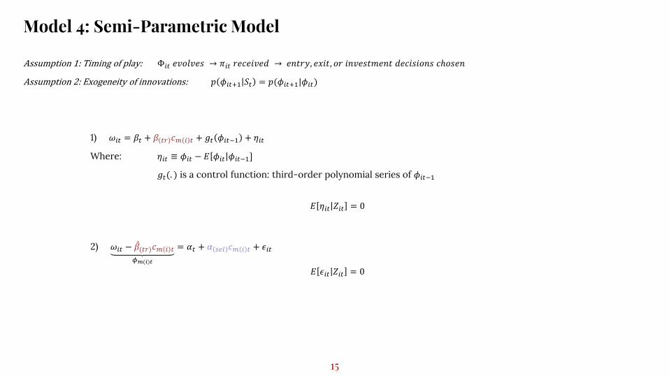
Assumption 1: Timing of play: Φ𝑖𝑡 𝑒𝑣𝑜𝑙𝑣𝑒𝑠 → 𝜋𝑖𝑡 𝑟𝑒𝑐𝑒𝑖𝑣𝑒𝑑 → 𝑒𝑛𝑡𝑟𝑦, 𝑒𝑥𝑖𝑡, 𝑜𝑟 𝑖𝑛𝑣𝑒𝑠𝑡𝑚𝑒𝑛𝑡 𝑑𝑒𝑐𝑖𝑠𝑖𝑜𝑛𝑠 𝑐ℎ𝑜𝑠𝑒𝑛

Assumption 2: Exogeneity of innovations: 𝑝 𝜙𝑖𝑡+1 𝑆𝑡 = 𝑝(𝜙𝑖𝑡+1|𝜙𝑖𝑡)

1) 𝜔𝑖𝑡 = 𝛽𝑡 + 𝛽 𝑡𝑟 𝑐𝑚 𝑖 𝑡 + 𝑔𝑡 𝜙𝑖𝑡−1 + 𝜂𝑖𝑡

Where: 𝜂𝑖𝑡 ≡ 𝜙𝑖𝑡 − 𝐸 𝜙𝑖𝑡 𝜙𝑖𝑡−1]

𝑔𝑡(. ) is a control function: third-order polynomial series of 𝜙𝑖𝑡−1

𝐸 𝜂𝑖𝑡 𝑍𝑖𝑡 = 0

2) 𝜔𝑖𝑡 − መ𝛽(𝑡𝑟)𝑐𝑚 𝑖 𝑡

𝜙𝑚(𝑖)𝑡

= 𝛼𝑡 + 𝛼 𝑠𝑒𝑙 𝑐𝑚 𝑖 𝑡 + 𝜖𝑖𝑡

𝐸 𝜖𝑖𝑡 𝑍𝑖𝑡 = 0

Model 4: Semi-Parametric Model

15

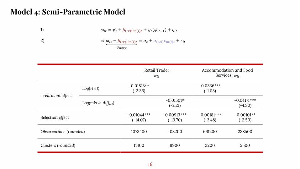
1) 𝜔𝑖𝑡 = 𝛽𝑡 + 𝛽 𝑡𝑟 𝑐𝑚 𝑖 𝑡 + 𝑔𝑡 𝜙𝑖𝑡−1 + 𝜂𝑖𝑡

2) ⇒ 𝜔𝑖𝑡 − መ𝛽(𝑡𝑟)𝑐𝑚 𝑖 𝑡

𝜙𝑚(𝑖)𝑡

= 𝛼𝑡 + 𝛼 𝑠𝑒𝑙 𝑐𝑚 𝑖 𝑡 + 𝜖𝑖𝑡

Model 4: Semi-Parametric Model

16

Retail Trade: 𝜔𝑖𝑡

Accommodation and Food Services: 𝜔𝑖𝑡

Treatment effect

Log(HHI) -0.01813**(-2.36)

-0.0336***(-1.03)

Log(mktsh difft-2)-0.01501*

(-2.21)-0.04171***

(-4.30)

Selection effect -0.01044***(-14.07)

-0.00913***(-19.70)

-0.00181***(-3.48)

-0.00101**(-2.50)

Observations (rounded) 1073400 403200 661200 238500

Clusters (rounded) 11400 9900 3200 2500

Appendix 1: Instrumental Variable Approach

17

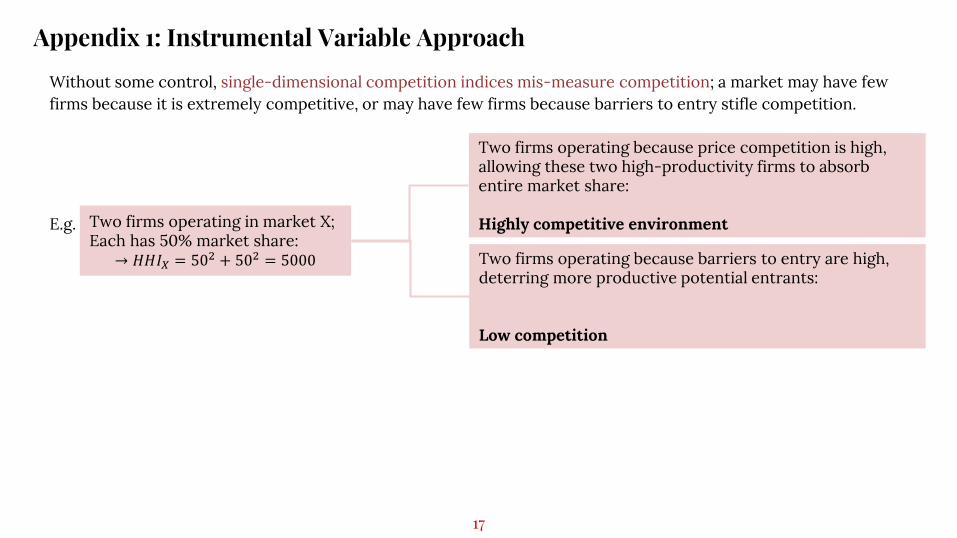
Without some control, single-dimensional competition indices mis-measure competition; a market may have few firms because it is extremely competitive, or may have few firms because barriers to entry stifle competition.

E.g. Two firms operating in market X;Each has 50% market share:

→ 𝐻𝐻𝐼𝑋 = 502 + 502 = 5000

Two firms operating because price competition is high, allowing these two high-productivity firms to absorb entire market share:

Highly competitive environment

Two firms operating because barriers to entry are high, deterring more productive potential entrants:

Low competition

Appendix 2: Grouped IV Quantile Model Approach

18

𝜔𝑖𝑡𝑘 = 𝛽𝑡

𝑘 + 𝛽𝑐𝑘𝑐𝑚𝑡 + 𝛽𝑋

𝑘𝑋𝑖𝑡𝑘 + 𝛾𝑖

𝑘 + 𝜁𝑖𝑘 + 𝛿𝑡

𝑘 + 𝜖𝑖𝑡

Aggregating to the market-level and comparing the effect of market competition on within-market productivity deciles:

The other approach would be to aggregate across markets.

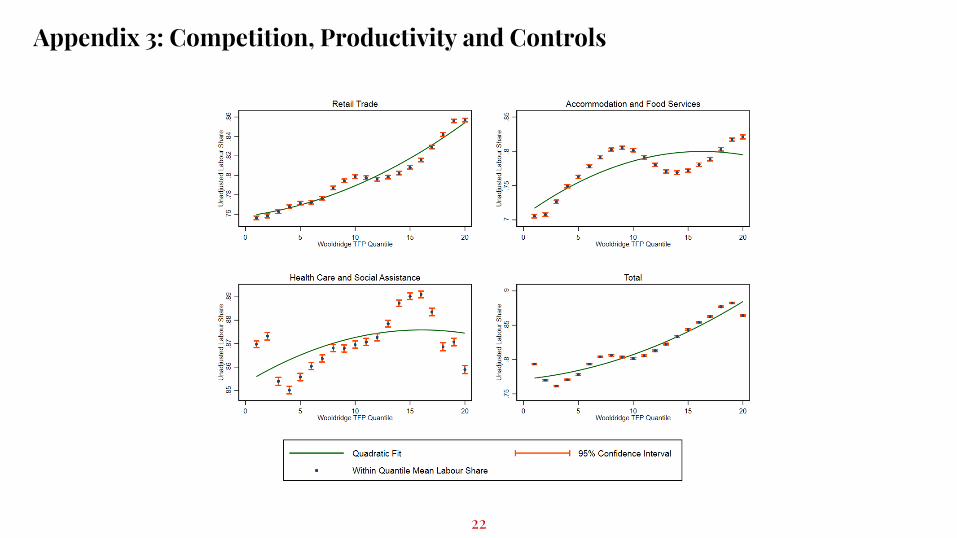
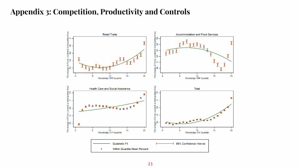
Appendix 3: Competition, Productivity and Controls

19

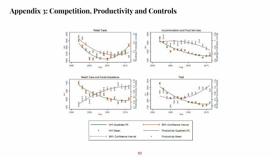
Appendix 3: Competition, Productivity and Controls

20

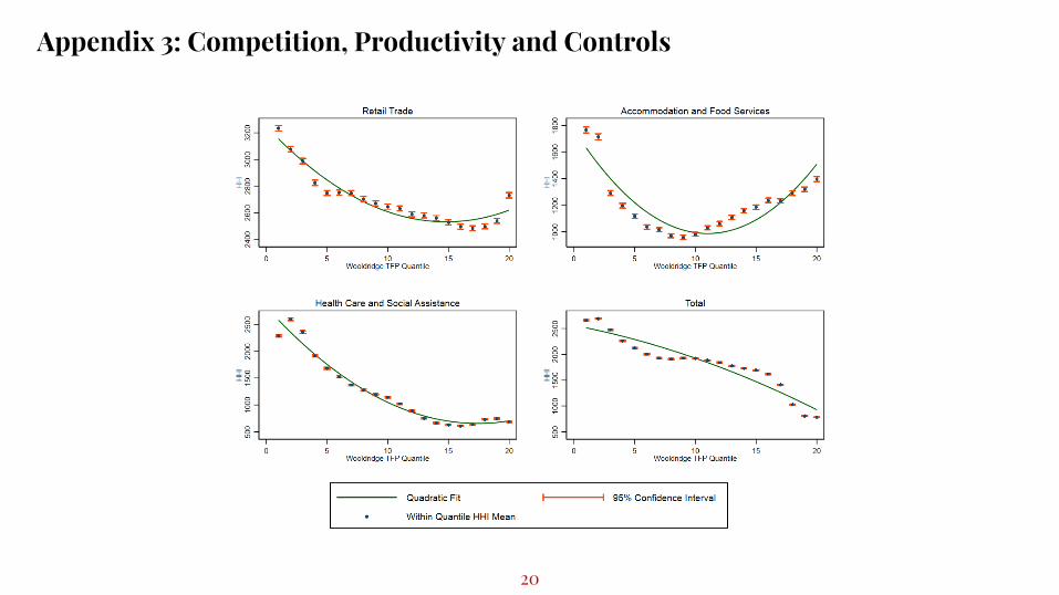
Appendix 3: Competition, Productivity and Controls

21

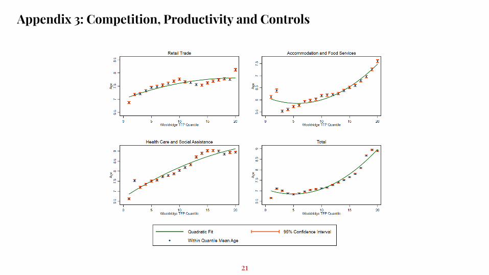
Appendix 3: Competition, Productivity and Controls

22

Appendix 3: Competition, Productivity and Controls

23

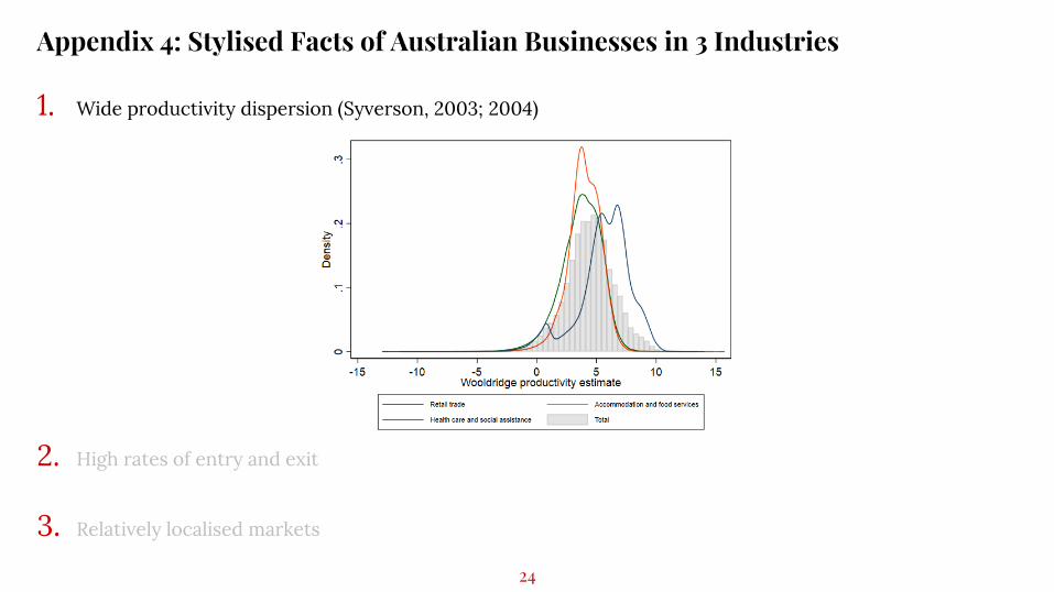
1. Wide productivity dispersion (Syverson, 2003; 2004)

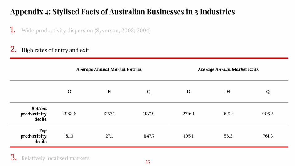
2. High rates of entry and exit

3. Relatively localised markets

Appendix 4: Stylised Facts of Australian Businesses in 3 Industries

24

1. Wide productivity dispersion (Syverson, 2003; 2004)

2. High rates of entry and exit

3. Relatively localised markets 25

Average Annual Market Entries Average Annual Market Exits

G H Q G H Q

Bottom productivity

decile2983.6 1257.1 1137.9 2716.1 999.4 905.5

Top productivity

decile81.3 27.1 1147.7 105.1 58.2 761.3

Appendix 4: Stylised Facts of Australian Businesses in 3 Industries

1. Wide productivity dispersion (Syverson, 2003; 2004)

2. High rates of entry and exit

3. Relatively localised markets

Identification for my empirical strategy relies on variation in market competition both cross-sectionally, and over time. I exploit postcode data in BLADE to create market definitions according to ABS Australian Statistical Geography Standard’s Statistical Area Level 3 (SA3).

26

Appendix 4: Stylised Facts of Australian Businesses in 3 Industries

Appendix 5: Background Literature

27

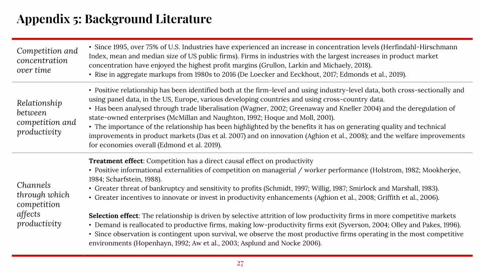
Competition and concentration over time

• Since 1995, over 75% of U.S. Industries have experienced an increase in concentration levels (Herfindahl-HirschmannIndex, mean and median size of US public firms). Firms in industries with the largest increases in product market concentration have enjoyed the highest profit margins (Grullon, Larkin and Michaely, 2018).• Rise in aggregate markups from 1980s to 2016 (De Loecker and Eeckhout, 2017; Edmonds et al., 2019).

Relationship between competition and productivity

• Positive relationship has been identified both at the firm-level and using industry-level data, both cross-sectionally and using panel data, in the US, Europe, various developing countries and using cross-country data. • Has been analysed through trade liberalisation (Wagner, 2002; Greenaway and Kneller 2004) and the deregulation of state-owned enterprises (McMillan and Naughton, 1992; Hoque and Moll, 2001).• The importance of the relationship has been highlighted by the benefits it has on generating quality and technical improvements in product markets (Das et al. 2007) and on innovation (Aghion et al., 2008); and the welfare improvements for economies overall (Edmond et al. 2019).

Channels through which competition affects productivity

Treatment effect: Competition has a direct causal effect on productivity• Positive informational externalities of competition on managerial / worker performance (Holstrom, 1982; Mookherjee, 1984; Scharfstein, 1988).• Greater threat of bankruptcy and sensitivity to profits (Schmidt, 1997; Willig, 1987; Smirlock and Marshall, 1983).• Greater incentives to innovate or invest in productivity enhancements (Aghion et al., 2008; Griffith et al., 2006).

Selection effect: The relationship is driven by selective attrition of low productivity firms in more competitive markets• Demand is reallocated to productive firms, making low-productivity firms exit (Syverson, 2004; Olley and Pakes, 1996).• Since observation is contingent upon survival, we observe the most productive firms operating in the most competitive environments (Hopenhayn, 1992; Aw et al., 2003; Asplund and Nocke 2006).

Note taking

28

This is your presentation title

Instructions for use

EDIT IN GOOGLE SLIDES

Click on the button under the presentation preview that says "Use as Google Slides Theme".

You will get a copy of this document on your Google Drive and will be able to edit, add or delete slides.

You have to be signed in to your Google account.

EDIT IN POWERPOINT®

Click on the button under the presentation preview that says "Download as PowerPoint template". You will get a .pptx file that you can edit in PowerPoint.

Remember to download and install the fonts used in this presentation (you’ll find the links to the font files needed in the Presentation design slide)

More info on how to use this template at www.slidescarnival.com/help-use-presentation-template

This template is free to use under Creative Commons Attribution license. You can keep the Credits slide or mention SlidesCarnival and other resources used in a slide footer.

30