
Ever thought of joining the CFA Program?
166
Ever thought of joining the CFA Program? As a CFA Institute Investment Foundations™ Program certificate holder, you can be justifiably proud of having made the effort to build your career and gain a clear understanding of the investment industry. We know that combining work with study is challenging, and it is likely that your employer and your colleagues appreciate and recognise your efforts. You may now feel more confident in your role as a result of being an Investment Foundations certificate holder, and you will certainly be a more valuable member of your organisation and the investment profession overall. The understanding you have gained of both the technical and ethical aspects of the profession are valuable to you, your employer, and to the investment industry. Most importantly, your acquired skills can help investors large and small to trust the investment industry and achieve their financial goals. Have you considered furthering your achievements? Some Investment Foundations certificate holders aspire to take the next step and study to obtain the CFA charter, the most respected and recognised investment management designation in the world. By becoming a CFA charterholder, you would also join CFA Institute, the world’s largest association of investment professionals. So is it for you? Only you can answer that. Most people who enroll in the CFA Program are looking to move to an investment management or research role or to enhance their skills in an existing investment role. More than 145,000 people, includ- ing some of the best-known names in the investment industry, now hold the CFA designation. However, getting there is not easy. Successful candidates take an average of four years to earn their CFA charter. The time and effort is substantial, and the learning is considerably more detailed and technical than the Investment Foundations course of study. Those of you who do enroll in the CFA Program will not do so lightly, so to help you decide if it’s for you, we have created a mini-curriculum to give you a taste of what to expect. The mini-curriculum comprises three sample topics from Level I of the CFA Program. You’ll notice that the format is similar to the Investment Foundations course of study: each chapter (or reading, as it is referred to in the CFA Program) is prefaced by Learning Outcome Statements to guide and focus your learning. Additionally, each reading contains questions to check your learning as you go along, as well as relevant examples and case studies. The mini-curriculum is designed to introduce you to key concepts in investing—qualitative and quantitative analysis. There is a reading on each, with a further reading designed to show how qualitative and quantitative techniques are often combined in investment. Don’t worry if you find the readings “dry” or don’t understand all of the information. Few candidates can absorb the material straight away, and there are plenty of online tools and other learning aids to assist candidates. But do ask yourself if you would like to understand it, whether you find the information interesting, and if it could be of use to you in your career. If you would like to take your career further and gain skills that could improve the investment profession, the CFA Program could be for you.
Transcript of Ever thought of joining the CFA Program?

Ever thought of joining the CFA Program?As a CFA Institute Investment Foundations™ Program certificate holder, you can be justifiably proud of having made the effort to build your career and gain a clear understanding of the investment industry. We know that combining work with study is challenging, and it is likely that your employer and your colleagues appreciate and recognise your efforts.
You may now feel more confident in your role as a result of being an Investment Foundations certificate holder, and you will certainly be a more valuable member of your organisation and the investment profession overall. The understanding you have gained of both the technical and ethical aspects of the profession are valuable to you, your employer, and to the investment industry. Most importantly, your acquired skills can help investors large and small to trust the investment industry and achieve their financial goals.
Have you considered furthering your achievements? Some Investment Foundations certificate holders aspire to take the next step and study to obtain the CFA charter, the most respected and recognised investment management designation in the world. By becoming a CFA charterholder, you would also join CFA Institute, the world’s largest association of investment professionals.
So is it for you? Only you can answer that. Most people who enroll in the CFA Program are looking to move to an investment management or research role or to enhance their skills in an existing investment role. More than 145,000 people, includ-ing some of the best- known names in the investment industry, now hold the CFA designation.
However, getting there is not easy. Successful candidates take an average of four years to earn their CFA charter. The time and effort is substantial, and the learning is considerably more detailed and technical than the Investment Foundations course of study. Those of you who do enroll in the CFA Program will not do so l ightly, so to help you decide if it’s for you, we have created a mini- curriculum to give you a taste of what to expect.
The mini-curriculum comprises three sample topics from Level I of the CFA Program. You’ll notice that the format is similar to the Investment Foundations course of study: each chapter (or reading, as it is referred to in the CFA Program) is prefaced by Learning Outcome Statements to guide and focus your learning. Additionally, each reading contains questions to check your learning as you go along, as well as relevant examples and case studies. The mini- curriculum is designed to introduce you to key concepts in investing—qualitative and quantitative analysis. There is a reading on each, with a further reading designed to show how qualitative and quantitative techniques are often combined in investment.
Don’t worry if you find the readings “dry” or don’t understand all of the information. Few candidates can absorb the material straight away, and there are plenty of online tools and other learning aids to assist candidates. But do ask yourself if you would like to understand it, whether you find the information interesting, and if it could be of use to you in your career.
If you would like to take your career further and gain skills that could improve the investment profession, the CFA Program could be for you.


Ethics and Trust in the
Investment Profession
by Bidhan L. Parmar, PhD, Dorothy C. Kelly, CFA, and
David B. Stevens, CFA
Bidhan L. Parmar, PhD, is at the University of Virginia (USA). Dorothy C. Kelly, CFA, is at
McIntire School of Commerce, University of Virginia (USA). David B. Stevens, CFA (USA).
LEARNING OUTCOMES
Mastery The candidate should be able to:
a. explain ethics;
b. describe the role of a code of ethics in defining a profession;
c. identify challenges to ethical behavior;
d. describe the need for high ethical standards in the investment
industry;
e. distinguish between ethical and legal standards;
f. describe and apply a framework for ethical decision making.
INTRODUCTION
As a candidate in the CFA Program, you are both expected and required to meet
high ethical standards. This reading introduces ideas and concepts that will help you
understand the importance of ethical behavior in the investment industry. You will
be introduced to various types of ethical issues within the investment profession and
learn about the CFA Institute Code of Ethics. Subsequently, you will be introduced
to a framework as a way to approach ethical decision making.
Imagine that you are employed in the research department of a large financial
services firm. You and your colleagues spend your days researching, analyzing, and
valuing the shares of publicly traded companies and sharing your investment recom-
mendations with clients. You love your work and take great satisfaction in knowing
that your recommendations can help the firm’s investing clients make informed invest-
ment decisions that will help them meet their financial goals and improve their lives.
1
R E A D I N G
1
© 2016 CFA Institute. All rights reserved.

Reading 1 ■ Ethics and Trust in the Investment Profession6
Several months after starting at the firm, you learn that an analyst at the firm has
been terminated for writing and publishing research reports that misrepresented the
fundamental risks of some companies to investors. You learn that the analyst wrote
the reports with the goal of pleasing the management of the companies that were
the subjects of the research reports. He hoped that these companies would hire your
firm’s investment banking division for its services and he would be rewarded with
large bonuses for helping the firm increase its investment banking fees. Some clients
bought shares based on the analyst’s reports and suffered losses. They posted stories
on the internet about their losses and the misleading nature of the reports. When
the media investigated and published the story, the firm’s reputation for investment
research suffered. Investors began to question the firm’s motives and the objectivity of
its research recommendations. The firm’s investment clients started to look elsewhere
for investment advice, and company clients begin to transfer their business to firms
with untarnished reputations. With business declining, management is forced to trim
staff. Along with many other hard- working colleagues, you lose your job—through
no fault of your own.
Imagine how you would feel in this situation. Most people would feel upset and
resentful that their hard and honest work was derailed by someone else’s unethical
behavior. Yet, this type of scenario is not uncommon. Around the world, unsuspecting
employees at such companies as SAC Capital, Stanford Financial Group, Everbright
Securities, Enron, Satyam Computer Services, Arthur Andersen, and other large com-
panies have experienced such career setbacks when someone else’s actions destroyed
trust in their companies and industries.
Businesses and financial markets thrive on trust—defined as a strong belief in
the reliability of a person or institution. In a 2013 study on trust, investors indicated
that to earn their trust, the top three attributes of an investment manager should be
that it (1) has transparent and open business practices, (2) takes responsible actions
to address an issue or crisis, and (3) has ethical business practices.1 Although these
attributes are valued by customers and clients in any industry, this reading will explore
why they are of particular importance to the investment industry.
People may think that ethical behavior is simply about following laws, regulations,
and other rules, but throughout our lives and careers we will encounter situations in
which there is no definitive rule that specifies how to act, or the rules that exist may be
unclear or even in conflict with each other. Responsible people, including investment
professionals, must be willing and able to identify potential ethical issues and create
solutions to them even in the absence of clearly stated rules.
ETHICS
Through our individual actions, each of us can affect the lives of others. Our decisions
and behavior can harm or benefit a variety of stakeholders—individuals or groups
of individuals who could be affected either directly or indirectly by a decision and
thus have an interest, or stake, in the decision. Examples of stakeholders in decisions
made by investment industry professionals include our colleagues, our clients, our
employers, the communities in which we live and work, the investment profession,
and other financial market participants. In some cases, our actions may benefit all of
these stakeholder groups; in other cases, our actions may benefit only some stakeholder
groups; and in still other cases, our actions may benefit some stakeholder groups and
2
1 CFA Institute and Edelman, “Investor Trust Study” (2013): http://www.cfapubs.org/doi/pdf/10.2469/
ccb.v2013.n14.1.

Ethics 7
harm others. For example, recall the research analyst in the introduction who wrote
misleading research reports with the aim of increasing the financial benefit to him-
self and his employer. In the very short term, his conduct seemed to directly benefit
some stakeholders (certain clients, himself, and his employer) and to harm other
stakeholders (clients who invested based on his reports). Over a longer time period,
his conduct resulted in harm to himself and many other stakeholders—his employer,
his employer’s clients, his colleagues, investors, and through loss of trust when the
story was published, the larger financial market.
Ethics encompasses a set of moral principles and rules of conduct that provide
guidance for our behavior. The word “ethics” comes from the Greek word “ethos,”
meaning character, used to describe the guiding beliefs or ideals characterizing a
society or societal group. Beliefs are assumptions or thoughts we hold to be true. A
principle is defined as a belief or fundamental truth that serves as the foundation for
a system of belief or behavior or a chain of reasoning. Our beliefs form our values—
those things we deem to have worth or merit.
Moral principles or ethical principles are beliefs regarding what is good, accept-
able, or obligatory behavior and what is bad, unacceptable, or forbidden behavior.
Ethical principles may refer to beliefs regarding behavior that an individual expects of
himself or herself, as well as shared beliefs regarding standards of behavior expected
or required by a community or societal group.
Another definition of ethics is the study of moral principles, which can be described
as the study of good and bad behavior or the study of making good choices as opposed
to bad choices. The study of ethics examines the role of consequences and personal
character in defining what is considered good, or ethical, conduct.
Ethical conduct is behavior that follows moral principles and balances self- interest
with both the direct and the indirect consequences of the behavior on others. Ethical
actions are those actions that are perceived as beneficial and conforming to the ethi-
cal expectations of society. An action may be considered beneficial if it improves the
outcomes or consequences for stakeholders affected by the action. Telling the truth
about the risks or costs associated with a recommended investment, for example, is
an ethical action—that is, one that conforms to the ethical expectations of society in
general and clients in particular. Telling the truth is also beneficial; telling the truth
builds trust with customers and clients and enables them to make more informed
decisions, which should lead to better outcomes for them and higher levels of client/
customer satisfaction for you and your employer.
Widely acknowledged ethical principles include honesty, fairness or justice, dili-
gence, and respect for the rights of others. Most societal groups share these fundamen-
tal ethical principles and build on them, establishing a shared set of rules regarding
how members should behave in certain situations. The principles or rules may take
different forms depending on the community establishing them.
Governments and related entities, for example, may establish laws and/or regula-
tions to reflect widely shared beliefs about obligatory and forbidden conduct. Laws and
regulations are rules of conduct specified by a governing body, such as a legislature
or a regulator, identifying how individuals and entities under its jurisdiction should
behave in certain situations. Most countries have laws and regulations governing the
investment industry and the conduct of its participants. Differences in laws may reflect
differences in beliefs and values.
In some countries, for example, the law requires that an investment adviser act
in the best interests of his or her clients. Other countries require that investment
professionals recommend investments that are suitable for their clients. Investment
advisers and portfolio managers who are required by law to act in their clients’ best
interests must always put their clients’ interests ahead of their own or their employ-
ers’ interests. An investment adviser who is required by law to act in a client’s best
interest must understand the client’s financial objectives and risk tolerance, research

Reading 1 ■ Ethics and Trust in the Investment Profession8
and investigate multiple investment opportunities, and recommend the investment
or investment portfolio that is most suitable for the client in terms of meeting his
or her long- term financial objectives. In addition, the investment adviser would be
expected to monitor the client’s financial situation and investments to ensure that
the investments recommended remain the best overall option for meeting the client’s
long- term financial objectives. In countries with only a suitability requirement, it is
legal for investment professionals to recommend a suitable investment to a client even
if other, similar suitable investments with lower fees are available. These differences
in laws reflect differences in beliefs and values.
Specific communities or societal groups in which we live and work sometimes cod-
ify their beliefs about obligatory and forbidden conduct in a written set of principles,
often called a code of ethics. Universities, employers, and professional associations
often adopt a code of ethics to communicate the organization’s values and overall
expectations regarding member behavior. The code of ethics serves as a general
guide for how community members should act. Some communities will also expand
on their codes of ethics and adopt explicit rules or standards that identify specific
behaviors required of community members. These standards of conduct serve as
benchmarks for the minimally acceptable behavior of community members and can
help clarify the code of ethics. Members can choose behaviors that demonstrate even
higher standards. By joining the community, members are agreeing to adhere to the
community’s code of ethics and standards of conduct. To promote their code of ethics
and reduce the incidence of violations, communities frequently display their codes in
prominent locations and in written materials. In addition, most communities require
that members commit to their codes in writing on an annual or more frequent basis.
Violations of a community’s established code of ethics and/or standards of con-
duct can harm the community in a variety of ways. Violations have the potential to
damage the community’s reputation among external stakeholders and the general
public. Violations can also damage the community’s reputation internally and lead to
reduced trust among community members and can cause the organization to fracture
or splinter from within. To protect the reputation of its membership and limit potential
harm to innocent members, the community may take corrective actions to investigate
possible violations, repair any damages, and attempt to discipline the violator or, in
severe cases, revoke the violator’s membership in the community.
CFA Institute is an example of a community with an established code of ethics
and standards of conduct. Its members and candidates commit to adhere to shared
beliefs about acceptable conduct for individuals participating in the investment indus-
try. These beliefs are presented in the Code of Ethics and Standards of Professional
Conduct (Code and Standards), which are included in the CFA Institute Standards of
Practice Handbook. The Code of Ethics communicates the organization’s principles,
values, and expectations. For example, the Code states that members and candidates
“place the integrity of the investment profession and the interests of clients above
their own personal interests.” The Standards of Professional Conduct outline mini-
mally acceptable behaviors expected of all CFA Institute members and candidates.
For example, one standard requires that “Members and Candidates must act for the
benefit of their clients and place their clients’ interests before their employer’s or their
own interests.” Another standard requires that “Members and Candidates must make
full and fair disclosure of all matters that could reasonably be expected to impair
their independence and objectivity or interfere with respective duties to their clients,
prospective clients, and employer. Members and Candidates must ensure that such
disclosures are prominent, are delivered in plain language, and communicate the
relevant information effectively.”
CFA Institute members and candidates re- affirm their commitment to adhere to the
Code and Standards each year. In addition, to protect the reputation of the community,
members and candidates agree to submit a Professional Conduct Statement each year

Ethics and Professionalism 9
disclosing conduct that may have violated the Code and Standards. To protect mem-
bers and candidates, CFA Institute has an established disciplinary process. Members
and candidates who violate the Code and Standards are subject to disciplinary action.
EXAMPLE 1
Ethics
1 Which of the following statements is most accurate? Ethics can be
described as:
A a commitment to upholding the law.
B an individual’s personal opinion about right and wrong.
C a set of moral principles that provide guidance for our behavior.
2 Which of the following statements is most accurate? Standards of conduct:
A are a necessary component of any code of ethics.
B serve as a general guide regarding proper conduct by members of a
group.
C serve as benchmarks for the minimally acceptable behavior required of
members of a group.
Solution to 1:
C is correct. Ethics can be described as a set of moral principles that provide
guidance for our behavior; these may be moral principles shared by a community
or societal group.
Solution to 2:
C is correct. Standards of conduct serve as benchmarks for the minimally
acceptable behavior required of members of a group. Some organizations will
adopt only a code of ethics, which communicates the organization’s values and
overall expectations regarding member behavior. Others may adopt both a
code of ethics and standards of conduct. Standards of conduct identify specific
behavior required of community members and serve as benchmarks for the
minimally acceptable behavior of community members.
ETHICS AND PROFESSIONALISM
As you progress in your career, you may find that attitudes among your peers vary:
Some of your peers may be happy to have a job, others may consider themselves fortu-
nate to find a vocation, and some may consider themselves part of a profession. What
are the differences? A job is very simply the work someone does to earn a living. A
vocation is a job or occupation to which someone is particularly well suited and is very
dedicated. Often, people will refer to a vocation as a calling: They work in service of a
cause they consider worthy. A profession is the ultimate evolution of an occupation,
resulting from the efforts of members practicing the occupation at a high level and
creating a set of ethics and standards of conduct for the entire group. A profession has
several characteristics that distinguish it from ordinary occupations. A profession is
1 based on specialized knowledge and skills.
3

Reading 1 ■ Ethics and Trust in the Investment Profession10
2 based on service to others.
3 practiced by members who share and agree to adhere to a common code of
ethics.
Professionals use their specialized knowledge and skills to serve their clients—with
whom they have a special relationship and to whom they have a special duty. Clients
differ from customers. A customer purchases goods or services in a single transaction
or series of transactions and pays for each transaction or series of transactions. A
client, in contrast, enters into an ongoing relationship with a professional, hiring the
professional to use his or her special knowledge for the benefit of the client, usually
for a fee. The relationship between client and professional is based on trust rather than
transactions. In exchange for the agreed- on fee, the professional accepts the duty to
place the client’s interests first at all times.
In any given profession, the code of ethics communicates the shared principles and
expected behaviors of its members. In addition to providing members with guidance for
decision making, a code of ethics may generate confidence among not only members
of the profession but also individuals who are not members of the profession, such as
clients, prospective clients, and/or the general public. The code of ethics informs and
provides some assurance to the public that the profession’s members will use their
specialized skills and knowledge in service of others.
Some codes will be enhanced and clarified by the adoption of standards of conduct
or specific benchmarks of behavior required of members. These standards may be
principle based or rule based. The CFA Institute Code and Standards are an example
of principle- based standards; they are based on the shared principles of honesty,
integrity, transparency, diligence, and placing client interests first. Rule- based stan-
dards are often narrowly defined, applying to specific groups of individuals in specific
circumstances. Principle- based standards, such as those of CFA Institute, apply to
all candidates and members at all times regardless of title, position, occupation, geo-
graphic location, or specific situation.
As a CFA Program candidate, you are expected to act in accordance with the
ethical and professional competency responsibilities of the investment profession as
expressed in the Code and Standards. The Code and Standards are designed to foster
and reinforce a culture of responsibility and professionalism. The Code and Standards
apply to all your professional activities, including but not limited to trading securities
for yourself and/or others, providing investment advice, conducting research, and
performing other investment services.
EXAMPLE 2
Ethics and Professionalism
1 Which of the following statements best describes how professionals use
their specialized knowledge and skills? Professionals use their specialized
knowledge and skills:
A in service to others.
B to advance their career.
C for the exclusive benefit of their employers.
2 Which of the following statements is most accurate? A profession’s code of
ethics:
A includes standards of conduct or specific benchmarks for behavior.

Challenges to Ethical Conduct 11
B ensures that all members of a profession will act ethically at all times.
C publicly communicates the shared principles and expected behaviors
of a profession’s members.
Solution to 1:
A is correct. Professionals use specialized knowledge and skills in service to
others. Their career and employer may benefit, but those results are not the pri-
mary focus of a professional’s use of his or her specialized knowledge and skills.
Solution to 2:
C is correct. A profession’s code of ethics publicly communicates the shared
principles and expected behaviors of a profession’s members. The existence
of a code of ethics does not ensure that all members will behave in a manner
consistent with the code and act ethically at all times. A profession will often
establish a disciplinary process to address alleged violations of the code of eth-
ics. A profession may adopt standards of conduct to enhance and clarify the
code of ethics.
CHALLENGES TO ETHICAL CONDUCT
Professionals generally aim to be responsible and to adhere to high moral standards, so
what is the benefit of studying ethics? Throughout our careers, we may find ourselves
in difficult or at least unfamiliar situations in which an appropriate course of action is
not immediately clear and/or there may be more than one seemingly acceptable choice;
studying ethics helps us prepare for such situations. This section addresses challenges
to engaging in ethical conduct. Failure to acknowledge, understand, or consider these
challenges can lead to poor decision making, resulting in unintentional consequences,
such as unethical conduct and potential violations of the Code and Standards.
Several challenges can make adherence to ethical conduct difficult. First, people
tend to believe that they are ethical people and that their ethical standards are higher
than average. Of course, everyone cannot be above average. However, surveys show
this belief in above averageness remains. As reported in A Crisis of Culture (2013), for
example, 71% of surveyed financial services executives rated their firm’s reputation for
ethical conduct better than the rest of the industry.2 Among those surveyed, 59% rated
the industry’s reputation for ethical conduct as positive. In contrast, a survey of global
consumer sentiment conducted the same year revealed that only 46% of consumers
surveyed trusted financial service providers to do the right thing.3 In fact, financial
services was the least trusted of all industries included in the survey.
These survey results illustrate overconfidence, a common behavioral bias that
can lead to faulty decision making. Studies have shown that our beliefs and emotions
frequently interfere with our cognitive reasoning and result in behavioral bias, a ten-
dency to behave in a way that is not strictly rational.4 As a result of the overconfidence
bias, we are more likely to overestimate the morality of our own behavior, particularly
in situations that we have not faced before. The overconfidence bias can result in a
4
2 Economist Intelligence Unit, “A Crisis of Culture: Valuing Ethics and Knowledge in Financial Services,”
Economist Intelligence Unit Report sponsored by CFA Institute (2013).
3 CFA Institute and Edelman, “Investor Trust Study” (2013): http://www.cfapubs.org/doi/pdf/10.2469/
ccb.v2013.n14.1.
4 Max H. Bazerman and Don A. Moore, Judgment in Managerial Decision Making, 8th ed. (Hoboken, NJ:
John Wiley & Sons, 2013).

Reading 1 ■ Ethics and Trust in the Investment Profession12
failure to consider, explicitly or implicitly, important inputs and variables needed to
form the best decision from an ethical perspective. In general, the overconfidence bias
leads us to place too much importance on internal traits and intrinsic motivations,
such as “I’m honest and would not lie,” even though studies have shown that internal
traits are generally not the main determinant of whether or not someone will behave
ethically in a given situation.5
A second challenge is that decision makers often fail to recognize and/or signifi-
cantly underestimate the effect of situational influences, such as what other people
around them are doing. Situational influences are external factors, such as environ-
mental or cultural elements, that shape our thinking, decision making, and behavior.
Social psychologists have studied how much situational influences affect our behavior
and have found that even good people with honorable motives can and often will be
influenced to do unethical things when put into difficult situations.6 Experiments have
shown that even people who consider themselves strong, independent, free thinkers
will conform to social pressures in many situations.7 The bystander effect, for example,
demonstrates that people are less likely to intervene in an emergency when others
are present. Fortunately, experiments have also shown that situational influences can
induce people to act more ethically. For example, people tend to behave more ethically
when they think someone else is watching or when there is a mirror placed close to
them.8 The important concept to understand is that situational influences have a very
powerful and often unrecognized effect on our thinking and behavior. Thus, learning
to recognize situational influences is critical to making good decisions.
Common situational influences in the investment industry that can shape think-
ing and behavior include money and prestige. One experiment found that simply
mentioning money can reduce ethical behavior. In the experiment, participants were
less likely to cooperate when playing a game if the game was called the Wall Street
Game, rather than the Community Game.9 In the investment industry, large financial
rewards—including individual salaries, bonuses, and/or investment gains—can induce
honest and well- intentioned individuals to act in ways that others might not consider
ethical. Large financial rewards and/or prestige can motivate individuals to act in their
own short- term self- interests, ignoring possible short- term risks or consequences to
themselves and others as well as long- term risks or consequences for both themselves
and others. Another extremely powerful situational influence is loyalty. Loyalty to
supervisors or organizations, fellow employees, and other colleagues can tempt indi-
viduals to make compromises and take actions that they would reject under different
situational influences or judge harshly when taken by others.
Situational influences often blind people to other important considerations.
Bonuses, promotions, prestige, and loyalty to employer and colleagues are examples
of situational influences that frequently have a disproportionate weight in our decision
making. Our brains more easily and quickly identify, recognize, and consider these
short- term situational influences than longer- term considerations, such as a commit-
ment to maintaining our integrity and contributing to the integrity of the financial
markets. Although absolutely important, these long- term considerations often have
5 Lee Ross and Richard E. Nisbett, The Person and the Situation: Perspectives of Social Psychology (New
York: McGraw- Hill, 1991).
6 Stanley Milgram, Obedience to Authority: An Experimental View (New York: Harper & Row, 1974).
7 Philip G. Zimbardo, The Power and Pathology of Imprisonment: Hearings Before Subcommittee No. 3 of
the Committee on the Judiciary, 92nd Congress, Corrections: Part II, Prisons, Prison Reform, and Prisoners’
Rights Congressional Record (Serial No. 15, 25 October 1971).
8 John M. Darley and C. Daniel Batson, “From Jerusalem to Jericho: A Study of Situational and Dispositional
Variables in Helping Behavior,” Journal of Personality and Social Psychology, vol., 27, no. 1 (1973): 100–108.
9 Varda Liberman, Steven M. Samuels, and Lee Ross, “The Name of the Game: Predictive Power of
Reputations versus Situational Labels in Determining Prisoner’s Dilemma Game Moves,” Personality and
Social Psychology Bulletin, vol. 30, no. 9 (September 2004): 1175–1185.

Challenges to Ethical Conduct 13
less immediate consequences than situational influences, making them less obvious
as factors to consider in a decision and, therefore, less likely to influence our overall
decision making. Situational influences shift our brain’s focus from the long term to
the short or immediate term. When our decision making is too narrowly focused on
short- term factors and/or self- interest, we tend to ignore and/or minimize the longer-
term risks and/or costs and consequences to ourselves and others, and the likelihood
of suffering ethical lapses and making poor decisions increases.
The story of Enron Corporation, a US energy company, illustrates the power
of situational influences. In the late 1990s, with approximately 20,000 employees,
the company’s culture focused on increasing current revenues and the share price
without regard for the long- term sustainability or consequences of such a culture.
Management received significant stock options, which provided strong motivation
to make decisions and take actions that would increase the share price. The focus on
share price was inescapable; employees were greeted by the stock ticker in lobbies
and elevators and on their computer screens. The focus on share price overshadowed
considerations about stakeholders and the long- term sustainability of the business
and its profits. Under these situational influences, some senior managers made poor
decisions and eventually succumbed to unethical conduct. They devised and adopted
complex accounting strategies that inflated revenues, obscured the company’s financial
performance, and hid billions of dollars in debt. In October 2001, the financial press
revealed what Enron’s accounting practices had previously concealed. Shares of Enron,
which had reached a high of US$90.75 in mid- 2000, fell to less than US$1 by the end of
November 2001. The company, which had claimed revenues of nearly US$111 billion
in 2000, secured a place in the record books as one of the largest bankruptcies in US
history. Dozens of former executives and employees were investigated, and many were
charged with fraud and/or conspiracy. Sixteen individuals pled guilty, including Chief
Financial Officer (CFO) Andrew S. Fastow, who pled guilty to conspiracy, forfeited
nearly US$30 million in cash and property, and was sentenced to six years in prison.
After a lengthy investigation and trial, former Chief Executive Officer Jeffrey K.
Skilling was convicted in May 2006 of fraud, conspiracy, insider trading, and making
false statements. He was sentenced to more than 24 years in prison, a sentence that
was eventually reduced to 14 years.10
Loyalty to employer and/or colleagues is an extremely powerful situational influence.
Our colleagues can influence our thinking and behavior in both positive and negative
ways. For example, colleagues may have encouraged you to signal your commitment
to your career and high ethical standards by enrolling in the CFA Program. If you
work for or with people who are not bound by the Code and Standards, they might
encourage you to take actions that are consistent with local law, unaware that the
recommended conduct falls short of the Code and Standards.
Well- intentioned firms may adopt or develop strong compliance programs to
encourage adherence to rules, regulations, and policies. A strong compliance policy
is a good start to developing an ethical culture, but a focus on adherence to rules
may not be sufficient. A compliance approach may not encourage decision makers
to consider the larger picture and can oversimplify decision making. Taken to the
extreme, a strong compliance culture can become another situational influence that
blinds employees to other important considerations. In a firm focused primarily on
compliance, employees may adopt a “check the box” mentality rather than an ethical
decision- making approach. Employees may ask the question “What can I do?” rather
than “What should I do?” At Enron, for example, in compliance with procedures, CFO
Fastow dutifully disclosed that he was the owner of several partnerships planning to
10 Chairman Kenneth M. Lay was also convicted of fraud, conspiracy, and making false statements. Lay
died on 5 July 2006 of heart failure while awaiting sentencing. Because he died before he could appeal the
verdict, the convictions were subsequently vacated.

Reading 1 ■ Ethics and Trust in the Investment Profession14
transact business with Enron. With powerful situational influences at work, Fastow
and board members focused on “What can I do?” rather than “What should I do?”
Compliance required that Fastow make the ownership disclosures and request approval
for the proposed business transactions from Enron’s board of directors, which he did.
Board members seemed to focus on the compliance requirements to provide board
approval of the proposed transactions rather than considering their obligations to
shareholders. In so doing, they neglected to view the issue from a broader perspec-
tive and consider “What should we do?” Consequently, they failed to recognize that
the proposed transactions placed Fastow’s interests in direct conflict with those of
his employer and its shareholders. By focusing on the compliance requirements to
provide board approval, board members failed to prevent Fastow from engaging in
activity that enriched himself at the expense of his employer and its shareholders. The
Enron case illustrates both the power of situational influences and the limitations of
a compliance approach, which can contribute to overconfidence and is insufficient
for ensuring ethical decision making,
EXAMPLE 3
Challenges to Ethical Conduct
1 Which of the following will most likely determine whether an individual
will behave unethically?
A The person’s character
B The person’s internal traits and intrinsic motivation
C External factors, such as environmental or cultural elements
2 Which of the following statements is most accurate?
A Large financial rewards, such as bonuses, are the most powerful situa-
tional influences.
B When decision making focuses on short- term factors, the likelihood of
ethical conduct increases.
C Situational influences can motivate individuals to act in their short-
term self- interests without recognizing the long- term risks or conse-
quences for themselves and others.
Solution to 1:
C is correct. Social psychologists have shown that even good people may behave
unethically in difficult situations. Situational influences, which are external fac-
tors (e.g., environmental or cultural elements), can shape our thinking, decision
making, and behavior and are more likely to lead to unethical behavior than
internal traits or character.
Solution to 2:
C is correct. Situational influences can motivate individuals to act in their short-
term self- interests without recognizing the long- term risks or consequences
for themselves and others. Large financial rewards are powerful situational
influences, but in some situations, other situational influences, such as loyalty
to colleagues, may be even more powerful.

The Importance of Ethical Conduct in the Investment Industry 15
THE IMPORTANCE OF ETHICAL CONDUCT IN THE
INVESTMENT INDUSTRY
Why are high ethical standards so important for the investment industry and invest-
ment professionals? As the global financial crisis of 2008 demonstrated, isolated and
seemingly unimportant individual decisions, such as approving loans to individuals
unable to provide proof of stable income, in aggregate can precipitate a market crisis
that can lead to economic difficulties and job losses for millions of individuals. In an
interconnected global economy and marketplace, each market participant must strive
to understand how his or her decisions and actions, and the products and services he
or she provides, may affect others not just in the short term but also the long term.
The investment industry serves society by matching those who supply capital, or
money, with those who seek capital to finance, or fund, their activities. For simplicity,
let us refer to those who supply capital as investors and those who seek capital as
borrowers. Borrowers may seek capital to achieve long- term goals, such as building or
upgrading factories, schools, bridges, highways, airports, railroads, or other facilities.
They may also seek short- term capital to fund short- term goals and/or support their
daily operations. Borrowers seeking capital to meet short- and long- term objectives
include sovereign entities, businesses, schools, hospitals, companies, and other
organizations that serve others. Some borrowers will turn to banks or other lending
institutions to finance their activities; others will turn to the financial markets to access
the funds they need to achieve their goals.
In exchange for supplying capital to fund the borrowers’ endeavors, investors
expect that their investments will generate returns that compensate them for the use
of their funds and the risks involved. Before providing capital, diligent and disciplined
investors will evaluate the risks and rewards of providing the capital. Some risks, such
as a downturn in the economy or a new competitor, could adversely affect the returns
expected from the investment. To help evaluate the potential risks and rewards of the
investment, investors conduct research, reading and evaluating the borrower’s finan-
cial statements, management’s business plan, research reports, industry reports, and
competitive analyses. Responsible investors will not invest their capital unless they
trust that their capital will be used in the way that has been described and is likely
to generate the returns they desire. Investors and society benefit when capital flows
to borrowers that can create the most value from the capital through their products
and services.
Capital flows more efficiently between investors and borrowers when financial
market participants are confident that all parties will behave ethically. Ethical behavior
builds and fosters trust, which has benefits for individuals, firms, the financial mar-
kets, and society. When people believe that a person or institution is reliable and acts
in accordance with their expectations, they are more willing to take risks involving
those people and institutions. For example, when people trust their financial advisers,
institutions, and the financial markets, they are more likely to invest their money and
accept the risk of short- term price fluctuations because they can reasonably believe
that their investments will provide them with long- term benefits. Entrepreneurs are
more likely to accept the risk of expanding their businesses, and hiring additional
employees, if they believe they will be able to attract investors with the funds needed
to expand at a reasonable cost. The higher the level of trust in the financial system, the
more people are willing to participate in the financial markets. Broad participation in
the financial markets enables the flow of capital to fund the growth in goods, services,
and infrastructure that benefits society with new and often better hospitals, bridges,
products, services, and jobs. Broad participation in the financial markets also means
5

Reading 1 ■ Ethics and Trust in the Investment Profession16
that the need and demand for investment professionals increase, resulting in more
job opportunities for those seeking to use their specialized skills and knowledge of
the financial markets in service to others.
Ethics always matter, but ethics are of particular importance in the investment
industry because the investment industry and financial markets are built on trust. Trust
is important to all business, yet it is especially important in the investment industry for
several reasons, including the nature of the client relationship, differences in knowl-
edge and access to information, and the nature of investment products and services.
In the client relationship, investors entrust their assets to financial firms for care
and safekeeping. By doing so, clients charge the firm and its employees with a special
responsibility; they are putting their faith and trust in the firm and its employees to
protect their assets. If the firm and its employees fail to protect clients’ assets, it could
have severe consequences for those clients. Without trust in that protection, the firm
and its employees would not have any business.
Those who work in the investment industry, as well as those who work in other
professions, have specialized knowledge and sometimes better access to information.
Having specialized knowledge and better access to information is an advantage in
any relationship, giving one party more power than the other. Investors trust that the
professionals they hire will not use their knowledge to take advantage of them. They
rely on the investment professional to use his or her specialized knowledge to serve
or benefit their clients’ interests.
Another reason why trust is so important in the investment industry has to do with
the nature of its products and services. In other industries—such as the transportation
industry, the technology industry, the retail industry, or the food industry—companies
produce products and/or provide services that are tangible and/or clearly visible.
We can hold an electronic tablet in our hands and inspect it. We can use software
programs, shop at retailers, dine at restaurant chains, and watch films. We can judge
the quality of the product or service based on a variety of factors: How well does it
perform its intended function? How efficient is it? How durable is it? How appealing
is it? Is the price reasonable or appropriate for the product or service?
In the investment industry, many investments are intangible and appear only as
numbers on a page or a screen. Investors cannot hold, inspect, or test their intended
purchases as they can a smartphone or a television set, each of which often come
with warranties should they fail to function as advertised. Without tangible products
to inspect, and with no warranties for protection should the product or service fail
to perform as expected, investors must rely on the information provided about the
investment—both before and after purchase. When they call their financial adviser
and ask to see their investments, they receive either an electronic or printed statement
with a list of holdings. They trust that the information is accurate and complete—a
fair representation—just as they trust that the investment professionals with whom
they are dealing will protect their interests. The globalization of finance also means
that investment professionals are likely to have business opportunities in new or
unfamiliar places. Without trust, financial transactions, including global transactions,
are less likely to occur.
Because of these factors, trust is the very foundation of the financial markets. This
trust is built, fostered, and maintained by the ethical actions of all the individuals who
work and/or participate in the markets, including those who work for companies,
banks, investment firms, sovereign entities, rating agencies, accounting firms, financial
advisers and planners, and institutional and retail investors. When market participants
act ethically, investors and others can trust that the numbers on the screen or the
page are accurate representations and be confident that investing and participating
in the financial markets is worthwhile.

Ethical vs. Legal Standards 17
Ethical behavior by all market participants can lead to broader participation in
the markets, protection of clients’ interests, and more opportunities for investment
professionals and their firms. Ethical behavior by firms can lead to higher levels of
success and profitability for the firms as well as their employees. Clients are attracted
to firms with trustworthy reputations, leading to more business, higher revenues,
and more profits. Ethical firms may also enjoy lower relative costs than unethical
firms because regulators are less likely to have cause to initiate costly investigations
or impose significant fines on firms in which high ethical standards are the norm.
Conversely, unethical behavior erodes and can even destroy trust. When clients
and investors suspect that they are not receiving accurate information or that the
market is not a level playing field, they lose trust. Investors with low trust are less
willing to accept risks. They may demand a higher return for the use of their capital,
choose to invest elsewhere, or choose not to invest at all. Any of these actions would
increase costs for borrowers seeking capital to finance their activities. Without access
to capital, borrowers may not be able to meet their goals of building new factories,
bridges, or hospitals. Decreases in investments can harm society by reducing jobs,
growth, and innovation. Unethical behavior ultimately harms not only clients, but
also the firm, its employees, and others.
Diminished trust in financial markets can reduce growth in the investment industry
and tarnish the reputation of firms and individuals in the industry, even if they did
not participate in the unethical behavior. Unethical behavior interferes with the ability
of markets to channel capital to the borrowers that can create the most value from
the capital, contributing to economic growth. Both markets and society suffer when
unethical behavior destroys trust in financial markets. For you personally, unethical
behavior can cost you your job, reputation, and professional stature and can lead to
monetary penalties and possibly time in jail.
EXAMPLE 4
The Importance of Ethical Conduct in the Investment
Industry
Which of the following statements is most accurate? Investment professionals
have a special responsibility to act ethically because:
A the industry is heavily regulated.
B they are entrusted to protect clients’ assets.
C the profession requires compliance with its code of ethics.
Solution:
B is correct. Investment professionals have a special responsibility because clients
entrust them to protect the clients’ assets.
ETHICAL VS. LEGAL STANDARDS
Many times, stakeholders have common ethical expectations. Other times, different
stakeholders will have different perceptions and perspectives and use different criteria
to decide whether something is beneficial and/or ethical.
Laws and regulations often codify ethical actions that lead to better outcomes for
society or specific groups of stakeholders. For example, some laws and regulations
require businesses and their representatives to tell the truth. They require specific
6

Reading 1 ■ Ethics and Trust in the Investment Profession18
written disclosures in marketing and other materials. Complying with such rules is
considered an ethical action; it creates a more satisfactory outcome that conforms to
stakeholders’ ethical expectations. As an example, consider disclosure requirements
mandated by securities regulators regarding the risks of investing. Complying with
such rules creates better outcomes for you, your clients, and your employer. First,
compliance with the rule reduces the risk that clients will invest in securities without
understanding the risks involved, which, in turn, reduces the risk that clients will file
complaints and/or take legal action if their investments decline in value. Complying
with the rules also reduces the risk that regulators will initiate an investigation, file
charges, or/and discipline or sanction you and/or your employer. Any of these actions
could jeopardize the reputation and future prospects of you and your employer. Conduct
that reduces these risks (e.g., following disclosure rules) would be considered ethical;
it leads to better outcomes for you, your clients, and your employer and conforms to
the ethical expectations of various stakeholders.
Although laws frequently codify ethical actions, legal and ethical conduct are not
always the same. Think about the diagram in Exhibit 1. Many types of conduct are
both legal and ethical, but some conduct may be one and not the other. Some legal
behaviors or activities may be considered unethical, and some behaviors or activi-
ties considered ethical may be deemed illegal in certain jurisdictions. Acts of civil
disobedience, such as peaceful protests, may be in response to laws that individuals
consider unethical. The act of civil disobedience may itself be considered ethical, and
yet it violates existing local laws.
The investment industry has examples of conduct that may be legal but considered
by some to be unethical. Some countries, for example, do not have laws prohibiting
trading while in possession of material nonpublic information, but many investment
professionals and CFA Institute consider such trading unethical.
Another area in which ethics and laws may conflict is the area of “whistleblowing.”
Whistleblowing refers to the disclosure by an individual of dishonest, corrupt, or
illegal activity by an organization or government. Depending on the circumstances,
a whistleblower may violate organizational policies and even local laws with the dis-
closure; thus, a whistleblower’s actions may be deemed illegal and yet considered by
some to be ethical.
Exhibit 1 Types of Conduct
LegalLegal
&Ethical
Ethical
Some people advocate that increased regulation and monitoring of the behavior
of participants in the investment industry will increase trust in the financial markets.
Although this approach may work in some circumstances, the law is not always the

Ethical vs. Legal Standards 19
best mechanism to reduce unethical behavior for several reasons. First, laws typically
follow market practices; regulators may proactively design laws and regulations to
address existing or anticipated practices that may adversely affect the fairness and
efficiency of markets or reactively design laws and regulations in response to a crisis
or an event that resulted in significant monetary losses and loss of confidence/trust
in the financial system. Regulators’ responses typically take significant time, during
which the problematic practice may continue or even grow. Once enacted, a new law
may be vague, conflicting, and/or too narrow in scope. A new law may reduce or even
eliminate the existing activity while simultaneously creating an opportunity for a dif-
ferent, but similarly problematic, activity. Additionally, laws vary across countries or
jurisdictions, allowing questionable practices to move to places that lack laws relevant
to the questionable practice. Laws are also subject to interpretation and compliance
by market participants, who may choose to interpret the law in the most advanta-
geous way possible or delay compliance until a later date. For these reasons, laws and
regulations are insufficient to ensure the ethical behavior of investment professionals
and market participants.
Ethical conduct goes beyond what is legally required and encompasses what dif-
ferent societal groups or communities, including professional associations, consider
to be ethically correct behavior. To act ethically, individuals need to be able to think
through the facts of the situation and make good choices even in the absence of clear
laws or rules. In many cases, there is no simple algorithm or formula that will always
lead to an ethical course of action. Ethics requires judgment—the ability to make
considered decisions and reach sensible conclusions. Good ethical judgment requires
actively considering the interests of stakeholders and trying to benefit multiple stake-
holders—clients, family, colleagues, employers, market participants, and so forth—and
minimize risks, including reputational risk.
EXAMPLE 5
Ethical vs. Legal Standards
1 Which of the following statements is most accurate?
A All legal behavior is ethical behavior.
B Some ethical behavior may be illegal.
C Legal standards represent the highest standard.
2 Which of the following statements is most accurate?
A Increased regulations are the most useful means to reduce unethical
behavior by market participants.
B Regulators quickly design and implement laws and regulations to
address practices that adversely affect the fairness and efficiency of
markets.
C New laws designed to reduce or eliminate conduct that adversely
affects the markets can create opportunities for different, but similarly
problematic, conduct.
Solution to 1:
B is correct. Some ethical behavior may be illegal. Civil disobedience is an exam-
ple of what may be illegal behavior that some consider to be ethical. Legal and
ethical behavior often coincide but not always. Standards of conduct based on
ethical principles may represent a higher standard of behavior than the behavior
required by law.

Reading 1 ■ Ethics and Trust in the Investment Profession20
Solution to 2:
C is correct. New laws designed to reduce or eliminate conduct that adversely
affects the markets can create opportunities for different, but similarly prob-
lematic, conduct.
ETHICAL DECISION- MAKING FRAMEWORKS
Laws, regulations, professional standards, and codes of ethics can guide ethical behav-
ior, but individual judgment is a critical ingredient in making principled choices and
engaging in appropriate conduct. One strategy to increase trust in the investment
industry is to increase the ability and motivation of market participants to act ethically
and help them minimize the likelihood of unethical actions. By integrating ethics into
the decision- making activities of employees, firms can enhance the ability and the
motivation of employees to act ethically, thereby reducing the likelihood of unethical
actions. The ability to relate an ethical decision- making framework to a firm’s or pro-
fession’s code of ethics allows investment professionals to bring the principles of the
code of ethics to life. An investment professional’s natural desire to “do the right thing”
can be reinforced by building a culture of integrity in the workplace. Development,
maintenance, and demonstration of a strong culture of integrity within the firm by
senior management may be the single most important factor in promoting ethical
behavior among the firm’s employees.
Adopting a code that clearly lays out the ethical principles that guide the thought
processes and conduct the firm expects from its employees is a critical first step. But
a code of ethics, although necessary, is insufficient. Simply nurturing an inclination to
do right is no match for the multitude of daily decisions that investment profession-
als make. We need to exercise ethical decision- making skills to develop the muscle
memory necessary for fundamentally ethical people to make good decisions despite
the reality of conflicts and our natural instinct for self- preservation. Just as coaching
and practice transform our natural ability to run across a field into the technique
and endurance required to run a race, teaching, reinforcing, and practicing ethical
decision- making skills prepare us to confront the hard issues effectively. It is good
for business, individuals, firms, the industry, and the markets, as well as society as a
whole, to engage in the investment management profession in a highly ethical manner.
A strong ethical culture that helps honest, ethical people engage in ethical behavior
will foster the trust of investors, lead to robust global financial markets, and ultimately
benefit society. That is why ethics matter.
When faced with decisions that can affect multiple stakeholders, investment
professionals must have a well- developed set of principles; otherwise, their thought
processes can lead to, at best, indecision and, at worst, fraudulent conduct and
destruction of the public trust. Establishing an ethical framework to guide your internal
thought process regarding how to act is a crucial step to engaging in ethical conduct.
Investment professionals are generally comfortable analyzing and making decisions
from an economic (profit/loss) perspective. Given the importance of ethical behavior
in carrying out professional responsibilities, it is also important to analyze decisions
and their potential consequences from an ethical perspective. Using a framework
for ethical decision making will help investment professionals to effectively examine
their choices in the context of conflicting interests common to their professional
obligations (e.g., researching and gathering information, developing investment
recommendations, and managing money for others). Such a framework will allow
investment professionals to analyze and choose options in a way that allows them
to meet high standards of ethical behavior. An ethical decision- making framework
7

Ethical Decision- Making Frameworks 21
provides investment professionals with a tool to help them adhere to a code of eth-
ics. By applying the framework and analyzing the particular circumstances of each
available alternative, investment professionals are able to determine the best course
of action to fulfill their responsibilities in an ethical manner.
An ethical decision- making framework will help a decision maker see the situation
from multiple perspectives and pay attention to aspects of the situation that may be
less evident with a short- term, self- focused perspective. The goal of getting a broader
picture of a situation is to be able to create a plan of action that is less likely to harm
stakeholders and more likely to benefit them. If a decision maker does not know or
understand the effects of his or her actions on stakeholders, the likelihood of making
a decision and taking action that harms stakeholders is more likely to occur, even if
unintentionally. Finally, an ethical decision- making framework helps decision makers
justify their actions to a broader audience of stakeholders.
Ethical decision- making frameworks are designed to facilitate the decision- making
process for all decisions. They help people look at and evaluate a decision from mul-
tiple perspectives, enabling them to identify important issues they might not oth-
erwise consider. Using an ethical decision- making framework consistently will help
you develop sound judgment and decision- making skills and avoid making decisions
that have unanticipated ethical consequences. Ethical decision- making frameworks
come in many forms with varying degrees of detail. A general ethical decision- making
framework is shown in Exhibit 2.
Exhibit 2 Ethical Decision- Making Framework
■ Identify: Relevant facts, stakeholders and duties owed, ethical principles,
conflicts of interest
■ Consider: Situational influences, additional guidance, alternative actions
■ Decide and act
■ Reflect: Was the outcome as anticipated? Why or why not?
The ethical decision- making process includes multiple phases, each of which has
multiple components. The process is often iterative, and you, the decision maker, may
move between phases in an order different from what is presented. For simplicity, we
will discuss the phases sequentially. In the initial phase, you will want to identify the
important facts that you have available to you, as well as information that you may
not have but would like to have to give yourself a more complete understanding of the
situation. You will also want to identify the stakeholders—clients, family, colleagues,
your employer, market participants, and so forth—and the duties you have to each of
them. You will then want to identify relevant ethical principles and/or legal require-
ments that might apply to the situation. You should also identify any potential conflicts
of interest inherent in the situation or conflicts in the duties you hold to others. For
example, your duty to your client may conflict with your duty to your employer.
In the second phase of ethical decision making, you will take time to consider
the situational influences as well as personal behavioral biases that could affect your
thinking and thus decision making. These situational influences and biases could
include a desire to please your boss, to be seen as successful by your peers and family,
to gain acceptance, to earn a large bonus, and so on. During this phase, you may seek
additional guidance from trusted sources—perhaps a family member, colleague, or
mentor who can help you think through the situation and help you identify and evaluate
alternative actions. You may turn to your compliance department for assistance or
you may even consult outside legal counsel. Seeking additional guidance is a critical

Reading 1 ■ Ethics and Trust in the Investment Profession22
step in viewing the situation from different perspectives. You should seek guidance
from someone who is not affected by the same situational influences and behavioral
biases as you are and can, therefore, provide a fresh perspective. You should also
seek guidance from your firm’s policies and procedures and the CFA Institute Code
and Standards. A helpful technique might be to imagine how an ethical peer or role
model might act in the situation.
The next phase of the framework is to make a decision and act. After you have
acted on your decision, you should take the time to reflect on and assess your deci-
sion and its outcome. Was the outcome what you anticipated? Why or why not? Had
you properly identified all the important facts, stakeholders, duties to stakeholders,
conflicts of interest, and relevant ethical principles? Had you considered the situa-
tional influences? Did you identify personal behavioral biases that might affect your
thinking? Had you sought sufficient guidance? Had you considered and properly
evaluated a variety of alternative actions? You may want to reflect on the decision
multiple times as the immediate and longer- term consequences of your decision and
actions become apparent.
The process is often iterative. After identifying the relevant facts and considering
situational influences, you may, for example, decide that you cannot make a decision
without more information. You may seek additional guidance on how to obtain the
information you need. You may also begin considering alternative actions regarding
how to proceed based on expectations of what the additional information will reveal,
or you may wait until you have more information, reflect on what you have done and
learned so far, and start the process over again. Sometimes cases can be complicated
and multiple iterations may reveal that no totally acceptable solution can be created.
Applying an ethical decision- making framework can help you evaluate the situation
so you can make the best possible decision. The next section shows applications of
the framework shown in Exhibit 2.
7.1 Applying the Framework
To illustrate how the framework could be applied in your career, consider the scenario
in Example 6.
EXAMPLE 6
Applying an Ethical Decision- Making Framework I
You have been hired as a junior analyst with a major investment bank. When
you join the bank, you receive a copy of the firm’s policies as well as training on
the policies. Your supervisor is the senior technology analyst for the investment
bank. As part of your duties, you gather information, draft documents, conduct
analysis, and perform other support functions for the senior analyst.
Your employer is one of several investment banks working on the initial
public offering (IPO) of a well- known technology company. The IPO is expected
to generate significant revenues for the investment banks participating in the
offering. The IPO has been highly anticipated and is in the news every day.
You are thrilled when your supervisor asks you to work on several research
projects related to analyzing and valuing the upcoming IPO for investors. You
eagerly compile information and draft a one- page outline. You stop to consider
what other information you could add to improve the report before proceeding.
You realize that you have two excellent contacts in the technology industry who
could review your work and provide some additional and potentially valuable
perspectives. You draft an email to your contacts reading:

Ethical Decision- Making Frameworks 23
I am working on an analysis and valuation of Big Tech Company for
investors. My employer is one of the banks participating in the IPO,
and I want to make sure I have considered everything. I was hoping
you could give me feedback on the prospects and risks facing Big
Tech. Please treat all the attached material as confidential.
Before hitting the send button, you stop and think about the ethical decision-
making framework you have studied. You decide to apply the framework and jot
down some notes as you work through the process: On the first page, you work
through the identification phase and make a list of the relevant facts, stakeholders
to whom you owe a duty, potential conflicts of interest, and ethical principles.
This list is shown is Exhibit 3.
Exhibit 3 Identification Phase
1 Relevant facts:
● Working on the deal/IPO of the decade
● Employer is one of several investment banks working on IPO
● The IPO is highly anticipated
● A successful IPO could lead to additional investment banking
deals and revenues for the firm
● Supervisor is relying on me
● Employer has documented policies and procedures
● Industry is regulated, with many rules and regulations in place
2 Stakeholders and duties owed. I have a duty to the following:
● Supervisor
● Employer
● Employer’s corporate client, the technology company
● Employer’s asset management and other investing clients
● Employer’s partners in the IPO
● Investors and market participants interested in the IPO
● All capital market participants
3 Conflicts or potential conflicts of interest include the following:
● Gathering additional research versus maintaining confidentiality
● Duty to supervisor versus desire to impress
● Duty to corporate client versus duty to other clients of the firm
● The firm’s corporate client benefits from a high IPO price whereas
the firm’s asset management clients would benefit from a low IPO
price
● Desire to work on more deals/IPOs versus objective analysis of the
investment potential of this deal
● My bonus, compensation, and career prospects are tied to my
supervisor’s and the IPO’s success; duty to employer
4 Ethical principles that are relevant to this situation include the
following:
● Duty of loyalty to employer
(continued)

Reading 1 ■ Ethics and Trust in the Investment Profession24
● Client interests come first
● Maintain confidences and confidentiality of information
On the next page, you write notes relating to the second phase of the frame-
work, considering the various situational factors and the guidance available to
you before considering alternative actions. These notes are shown in Exhibit 4.
Exhibit 4 Consideration Phase
1 Situational influences:
● The firm’s written policies
● The bank will earn big fees from the IPO
● I want to impress my boss—and potential future bosses
● My bonus, compensation, and career prospects will be influenced
by my contribution to this deal and other deals
● I am one of very few people working on this deal; it is a real
honor, and others would be impressed that I am working on this
deal
● My employer is filled with successful and wealthy people who are
go- getters; I want to be successful and wealthy like them
2 Additional guidance. I could seek guidance from the following:
● The firm’s code of ethics
● The firm’s written policies
● A peer in my firm
● My supervisor, the senior analyst
● The compliance department
● A mentor either at the firm or perhaps from university
● The CFA Institute Code and Standards
3 Alternative actions. I could consider the following:
● Asking contacts what they have heard
● Submitting the report as a draft and suggesting that contacts in
the industry might be able to provide more perspective
● Sending a survey to various technology industry veterans soliciting
their viewpoints on developments
After completing these steps, you decide to check the firm’s policies. Under
a section entitled “Research Analyst Role in Securities Offerings,” the manual
states, “You may not distribute any written (which include email, fax, electronic,
and other means) material related to companies and/or their offerings. . . during
the course of any offering and the related quiet period.”
You read further and note a section entitled “Wall Crossing Policy and
Procedures” that states that “employees with confidential information may not
communicate the information to anyone who does not have a valid need to know”
without first obtaining clearance from the legal and compliance department.
Exhibit 3 (Continued)

Ethical Decision- Making Frameworks 25
You decide that your contacts do not have a “valid need to know” and that it
is unlikely the firm’s legal and compliance professionals would approve sharing
the information. You then decide to mention your contacts to the senior research
analyst. He suggests that they may have some useful perspective and that you
might talk to them to hear their perspective and cautions you not to disclose
any information about any of the firm’s clients, pending deals, or research. You
return to your desk, delete the email, and following the senior research analyst’s
advice, call your contacts on the telephone to discuss the technology sector, its
prospects, and its challenges. During the calls, you take care not to reveal any
details about Big Tech Company or its offering.
Whatever action you take, you should take time afterward to reflect on the
decision and the outcome. Was the outcome as anticipated? Why or why not?
The initial facts presented in the example are based on the real- life experience of
a young junior analyst working on a highly anticipated IPO. The junior analyst may
or may not have used an ethical decision- making framework to evaluate his situation.
Without seeking additional guidance, the junior analyst sent an email similar to the
one in the example with an attachment that included confidential, proprietary infor-
mation, including the senior analyst’s analysis and forecasts. Months later, long after
the IPO offering, the junior analyst’s email was discovered by his employer. When
questioned, he admitted that he had received training regarding the firm’s policies
and that he did not discuss or seek approval from anyone before sending the email.
Two days later, the firm terminated the junior analyst’s employment and reported to
regulatory authorities that he had been terminated for distributing written materials,
by email, during a securities offering in violation of firm policies that prohibit the
dissemination of any written materials during the course of a securities offering and
related periods. The junior analyst’s supervisor also lost his job for failing to properly
supervise the analyst. Multiple regulators investigated the matter, and the firm was
fined millions of dollars for failing to supervise its employees properly. The information
regarding the junior analyst’s termination was posted and remains available on the
regulator’s website for all to see. Future employers conducting routine background
checks will know that the analyst was terminated for violating firm policies relating
to a securities offering.
The example presented is similar to situations faced by many analysts. Using an
ethical decision- making framework will help you evaluate situations from multiple
perspectives, avoid poor decision making, and avoid the consequences that can result
from taking an ill- conceived course of action. Using an ethical decision- making
framework is no guarantee of a positive outcome but may help you avoid making
unethical decisions.
EXAMPLE 7
Applying an Ethical Decision- Making Framework II
A financial adviser has been saving a portion of his salary to purchase a new
vehicle. He is on track to have enough saved within the next three months. His
employer has offered a special bonus for this quarter, which will go to the team
that attracts the most new investors into the firm’s investment funds. In addi-
tion to the potential bonus, the firm pays a 5% commission to employees who
sell shares in the firm’s investment funds. Several of the funds are highly rated,
including one designed to provide steady income to investors.

Reading 1 ■ Ethics and Trust in the Investment Profession26
The financial adviser has added only a few new investors to the firm’s funds,
but his teammates have been very successful in their efforts. The end of the
quarter is one week away, and his team is competing closely with another team
for the bonus. One of his teammates informs the financial adviser that he really
needs the bonus so his elderly mother can receive medical treatment.
Later that day, the financial adviser meets with an elderly client on a limited
income who is seeking more income from his investment portfolio. The client
is 89 years old and in poor health. According to the client’s will, the client’s
investment portfolio will go to his favorite charity upon his death.
1 Which of the following situational influences is likely to have the most
effect on the financial adviser’s efforts to get new clients to invest in the
funds? His relationship with his:
A client.
B employer.
C teammates.
2 Which of the following statements is most accurate? An ethical decision-
making framework:
A is only beneficial when a firm lacks a code of ethics.
B is used to improve compliance with laws and regulations.
C is a tool for analyzing the potential alternative actions and conse-
quences of a decision.
3 Which of the following is most accurate? Ethical decision- making
frameworks:
A raise awareness of different perspectives.
B focus attention on short- term consequences.
C allocate more weight to those who will directly benefit from the
decision.
4 Which of the following is most accurate? Ethical decision- making
frameworks:
A are not needed if behavior is legal.
B identify who gains the most from a decision.
C can help reduce unanticipated ethical lapses and unexpected
consequences.
5 Using an ethical decision- making framework, which of the following
duties would most likely take precedence in the scenario described? The
financial adviser’s duty to his:
A client.
B employer.
C colleagues.
6 Using an ethical decision- making framework, the financial adviser would
most likely:
A recommend that the elderly client invest at least some of his assets in
the highly rated fund.
B research other investments that can provide steady income before
making a recommendation to his elderly client.
C disclose the commission he would earn before recommending that the
elderly client invest at least some of his assets in the highly rated fund.

Conclusion 27
Solution to 1:
C is correct. The financial adviser’s relationship with his teammates is likely to
have the most effect on the financial adviser’s efforts.
Solution to 2:
C is correct. An ethical decision- making framework is a tool for analyzing the
potential alternative actions and consequences of a decision.
Solution to 3:
A is correct. Ethical decision- making frameworks raise awareness of different
perspectives.
Solution to 4:
C is correct. Ethical decision- making frameworks can help avoid unanticipated
ethical consequences.
Solution to 5:
A is correct. Using an ethical decision- making framework, the financial adviser’s
relationship with his client would most likely take precedence in this scenario.
The adviser should put his client’s interests first. The exception to client inter-
ests taking precedence occurs when market integrity effects take precedence.
Solution to 6:
B is correct. Using an ethical decision- making framework, the financial adviser
would identify the relevant facts, stakeholders, duties owed, and potential con-
flicts. In this scenario, the financial adviser owes a duty to his client as well as
his employer. His client’s interests take precedence over all other interests. The
bonus and his colleague’s desire to help his mother are situational influences. To
navigate this situation, the financial adviser should seek additional information;
he should research the risk and return parameters and fee structures of other
investments that can provide steady income before making a recommendation
to his client.
CONCLUSION
This reading introduced ideas and concepts that will help you understand the impor-
tance of ethical behavior in the investment industry as well as the challenges to adhering
to high ethical standards. A code of ethics will communicate an organization’s values
and the expected behavior of its members as well as provide guidance for decision
making. A code of ethics may be further enhanced and clarified by the adoption of
standards of conduct. An ethical decision- making framework combined with a code
of ethics may help investment professionals analyze their decisions in a way that
identifies potential conflicts and negative consequences.
Knowing the rules to apply in a particular situation, although important, may not
be sufficient to ensure ethical conduct if used alone. Responsible professionals in the
investment industry must be able both to recognize areas that are prone to ethical
pitfalls and to identify and process those circumstances and influences that can impair
judgment and lead to ethical lapses.
8

Reading 1 ■ Ethics and Trust in the Investment Profession28
SUMMARY
■ Ethics refers to the study of making good choices. Ethics encompasses a set of
moral principles and rules of conduct that provide guidance for our behavior.
■ Situational influences are external factors that may shape our behavior.
■ Challenges to ethical behavior include being overconfident in our own morality,
underestimating the effect of situational influences, and focusing on the imme-
diate rather than long- term outcomes or consequences of a decision.
■ In any given profession, the code of ethics publicly communicates the estab-
lished principles and expected behavior of its members.
■ Members of a profession use specialized knowledge and skills to serve others;
they share and agree to adhere to a common code of ethics to serve others and
advance the profession.
■ A code of ethics helps foster public confidence that members of the profession
will use their specialized skills and knowledge to serve their clients and others.
■ High ethical standards always matter and are of particular importance in the
investment industry, which is based almost entirely on trust. Clients trust
investment professionals to use their specialized skills and knowledge to serve
clients and protect client assets. All stakeholders gain long- term benefits when
investment professionals adhere to high ethical standards.
■ Rules and laws often codify ethical actions that lead to better outcomes for soci-
ety or specific groups of stakeholders.
■ Organizations and individuals generally adhere to legal standards, but legal
standards are often created to address past ethical failings and do not provide
guidance for an evolving and increasingly complex world.
■ Legal standards are often rule based. Ethical conduct goes beyond legal stan-
dards, balancing self- interest with the direct and indirect consequences of
behavior on others.
■ A framework for ethical decision making can help people look at and evaluate a
decision from different perspectives, enabling them to identify important issues,
make wise decisions, and limit unintended consequences.

Practice Problems 29
PRACTICE PROBLEMS
1 Benchmarks for minimally acceptable behaviors of community members are:
A a code of ethics.
B laws and regulations.
C standards of conduct.
2 Specialized knowledge and skills, a commitment to serve others, and a shared
code of ethics best characterize a(n):
A vocation.
B profession.
C occupation.
3 Which of the following best identifies an internal trait that may lead to poor
ethical decision making?
A Overconfidence
B Loyalty to employer
C Promise of money or prestige
4 Situational influences in decision making will most likely be minimized if:
A strong compliance programs are in place.
B longer- term consequences are considered.
C individuals believe they are truthful and honest.
5 Decision makers who use a compliance approach are most likely to:
A avoid situational influences.
B oversimplify decision making.
C consider more factors than when using an ethical decision- making
approach.
6 When unethical behavior erodes trust in an investment firm, that firm is more
likely to experience:
A lower revenues only.
B higher expenses only.
C lower revenues and higher expenses.
7 Which is an example of an activity that may be legal but that CFA Institute
considers unethical?
A Making legally required disclosures in marketing materials
B Trading while in possession of material nonpublic information
C Disclosure by an employee of his or her own company’s dishonest activity
8 An ethical decision- making framework will most likely:
A include a pre- determined, uniform sequence.
B focus exclusively on confirmable facts and relationships.
C help avoid a decision that has unanticipated ethical consequences.
© 2017 CFA Institute. All rights reserved.

Reading 1 ■ Ethics and Trust in the Investment Profession30
SOLUTIONS
1 C is correct. Standards of conduct are applied to specific communities or soci-
etal groups and identify specific behaviors required of community members.
These standards of conduct serve as benchmarks for the minimally acceptable
behavior of community members. Codes of ethics serve as a general guide for
how community members should act; they communicate the organization’s
values and overall expectations regarding member behavior, but they do not
identify specific behaviors required of community members. Laws and regu-
lations are rules of conduct defined by governments and related entities about
obligatory and forbidden conduct broadly applicable for individuals and entities
under their jurisdiction.
2 B is correct. A profession has several characteristics that distinguish it from
an occupation or vocation, such as specialized knowledge and skills, service to
others, and a code of ethics shared by its members. A profession is the ultimate
evolution of an occupation, resulting from excellence in practice and expected
adherence to a code of ethics and standards of practice.
3 A is correct. An overconfidence bias can lead individuals to put too much
importance on internal traits and intrinsic motivations, such as their own per-
ceptions of personal honesty, that can lead to faulty decision making. Loyalty
to an employer and promise of money or prestige are situational influences that
can lead to faulty decision making.
4 B is correct. Consciously considering long- term consequences will help off-
set situational influences. We more easily recognize and consider short- term
situational influences than longer- term considerations because longer- term
considerations have fewer immediate consequences than situational influences
do. When decision making is too narrowly focused on short- term factors, we
tend to ignore longer- term risks and consequences, and the likelihood of poor
ethical decision making increases. A strong compliance policy is a good first
step toward developing an ethical culture; a focus on rules adherence may not
be sufficient. Emphasis on compliance may not encourage decision makers to
consider the larger picture and can oversimplify decision making. Taken to the
extreme, a strong compliance culture can become another situational influence
that blinds employees to other important considerations. An overconfidence
bias can place too much importance on internal traits and intrinsic motivations,
such as “I’m honest and would not lie,” even though studies have shown that
internal traits are generally not the main determinant of whether or not some-
one will behave ethically in a given situation.
5 B is correct. A compliance approach can oversimplify decision making and may
not encourage decision makers to consider the larger picture. A strong com-
pliance culture may be a good start in developing an ethical culture but can
become another situational influence that may result in employees failing to
consider other important factors.
6 C is correct. Unethical behavior ultimately harms investment firms. Clients are
not attracted if they suspect unethical behavior, leading to less business and
lower revenues. Investment firms may also experience higher relative costs
because regulators are more likely to have cause to initiate costly investigations.

Solutions 31
7 B is correct. The investment industry has examples of conduct that may be
legal but that CFA Institute considers unethical. Trading while in possession
of material nonpublic information is not prohibited by law worldwide and can,
therefore, be legal, but CFA Institute considers such trading unethical.
8 C is correct. Using an ethical decision- making framework consistently will help
you develop sound judgment and decision- making skills and avoid making
decisions that have unanticipated ethical consequences. The decision- making
process is often iterative, and the decision maker may move between phases of
the framework. A decision maker should consider more than confirmable facts
and relationships; for example, the decision maker should consider situational
influences and personal biases.


Statistical Concepts and Market Returns
by Richard A. DeFusco, PhD, CFA, Dennis W. McLeavey, CFA,
Jerald E. Pinto, PhD, CFA, and David E. Runkle, PhD, CFA
Richard A. DeFusco, PhD, CFA, is at the University of Lincoln- Nebraska (USA). Dennis W.
McLeavey, CFA, is at the University of Rhode Island (USA). Jerald E. Pinto, PhD, CFA, is
at CFA Institute (USA). David E. Runkle, PhD, CFA, is at Trilogy Global Advisors (USA).
LEARNING OUTCOMES
Mastery The candidate should be able to:
a. distinguish between descriptive statistics and inferential statistics,
between a population and a sample, and among the types of
measurement scales;
b. define a parameter, a sample statistic, and a frequency
distribution;
c. calculate and interpret relative frequencies and cumulative
relative frequencies, given a frequency distribution;
d. describe the properties of a data set presented as a histogram or a
frequency polygon;
e. calculate and interpret measures of central tendency, including
the population mean, sample mean, arithmetic mean, weighted
average or mean, geometric mean, harmonic mean, median, and
mode;
f. calculate and interpret quartiles, quintiles, deciles, and
percentiles;
g. calculate and interpret 1) a range and a mean absolute deviation
and 2) the variance and standard deviation of a population and of
a sample;
h. calculate and interpret the proportion of observations falling
within a specified number of standard deviations of the mean
using Chebyshev’s inequality;
i. calculate and interpret the coefficient of variation and the Sharpe
ratio;
j. explain skewness and the meaning of a positively or negatively
skewed return distribution;
(continued)
R E A D I N G
8
© 2014 CFA Institute. All rights reserved.

Reading 8 ■ Statistical Concepts and Market Returns390
LEARNING OUTCOMES
Mastery The candidate should be able to:
k. describe the relative locations of the mean, median, and mode for
a unimodal, nonsymmetrical distribution;
l. explain measures of sample skewness and kurtosis;
m. compare the use of arithmetic and geometric means when
analyzing investment returns.
INTRODUCTION
Statistical methods provide a powerful set of tools for analyzing data and drawing
conclusions from them. Whether we are analyzing asset returns, earnings growth
rates, commodity prices, or any other financial data, statistical tools help us quantify
and communicate the data’s important features. This reading presents the basics of
describing and analyzing data, the branch of statistics known as descriptive statis-
tics. The reading supplies a set of useful concepts and tools, illustrated in a variety of
investment contexts. One theme of our presentation, reflected in the reading’s title,
is the demonstration of the statistical methods that allow us to summarize return
distributions.1 We explore four properties of return distributions:
■ where the returns are centered (central tendency);
■ how far returns are dispersed from their center (dispersion);
■ whether the distribution of returns is symmetrically shaped or lopsided (skew-
ness); and
■ whether extreme outcomes are likely (kurtosis).
These same concepts are generally applicable to the distributions of other types of
data, too.
The reading is organized as follows. After defining some basic concepts in Section
2, in Sections 3 and 4 we discuss the presentation of data: Section 3 describes the
organization of data in a table format, and Section 4 describes the graphic presenta-
tion of data. We then turn to the quantitative description of how data are distributed:
Section 5 focuses on measures that quantify where data are centered, or measures of
central tendency. Section 6 presents other measures that describe the location of data.
Section 7 presents measures that quantify the degree to which data are dispersed.
Sections 8 and 9 describe additional measures that provide a more accurate picture of
data. Section 10 provides investment applications of concepts introduced in Section 5.
SOME FUNDAMENTAL CONCEPTS
Before starting the study of statistics with this reading, it may be helpful to examine a
picture of the overall field. In the following, we briefly describe the scope of statistics
and its branches of study. We explain the concepts of population and sample. Data
1
2
1 Ibbotson Associates (www.ibbotson.com) generously provided some of the data used in this reading.
We also draw on Dimson, Marsh, and Staunton’s (2011) history and study of world markets as well as
other sources.

Some Fundamental Concepts 391
come in a variety of types, affecting the ways they can be measured and the appro-
priate statistical methods for analyzing them. We conclude by discussing the basic
types of data measurement.
2.1 The Nature of Statistics
The term statistics can have two broad meanings, one referring to data and the other
to method. A company’s average earnings per share (EPS) for the last 20 quarters, or
its average returns for the past 10 years, are statistics. We may also analyze historical
EPS to forecast future EPS, or use the company’s past returns to infer its risk. The
totality of methods we employ to collect and analyze data is also called statistics.
Statistical methods include descriptive statistics and statistical inference (infer-
ential statistics). Descriptive statistics is the study of how data can be summarized
effectively to describe the important aspects of large data sets. By consolidating a
mass of numerical details, descriptive statistics turns data into information. Statistical
inference involves making forecasts, estimates, or judgments about a larger group
from the smaller group actually observed. The foundation for statistical inference is
probability theory, and both statistical inference and probability theory will be dis-
cussed in later readings. Our focus in this reading is solely on descriptive statistics.
2.2 Populations and Samples
Throughout the study of statistics we make a critical distinction between a population
and a sample. In this section, we explain these two terms as well as the related terms
“parameter” and “sample statistic.”2
■ Definition of Population. A population is defined as all members of a speci-
fied group.
Any descriptive measure of a population characteristic is called a parameter.
Although a population can have many parameters, investment analysts are usually
concerned with only a few, such as the mean value, the range of investment returns,
and the variance.
Even if it is possible to observe all the members of a population, it is often too
expensive in terms of time or money to attempt to do so. For example, if the popu-
lation is all telecommunications customers worldwide and an analyst is interested in
their purchasing plans, she will find it too costly to observe the entire population. The
analyst can address this situation by taking a sample of the population.
■ Definition of Sample. A sample is a subset of a population.
In taking a sample, the analyst hopes it is characteristic of the population. The field
of statistics known as sampling deals with taking samples in appropriate ways to
achieve the objective of representing the population well. A later reading addresses
the details of sampling.
Earlier, we mentioned statistics in the sense of referring to data. Just as a parameter
is a descriptive measure of a population characteristic, a sample statistic (statistic, for
short) is a descriptive measure of a sample characteristic.
■ Definition of Sample Statistic. A sample statistic (or statistic) is a quantity
computed from or used to describe a sample.
2 This reading introduces many statistical concepts and formulas. To make it easy to locate them, we have
set off some of the more important ones with bullet points.

Reading 8 ■ Statistical Concepts and Market Returns392
We devote much of this reading to explaining and illustrating the use of statistics
in this sense. The concept is critical also in statistical inference, which addresses such
problems as estimating an unknown population parameter using a sample statistic.
2.3 Measurement Scales
To choose the appropriate statistical methods for summarizing and analyzing data,
we need to distinguish among different measurement scales or levels of measure-
ment. All data measurements are taken on one of four major scales: nominal, ordinal,
interval, or ratio.
Nominal scales represent the weakest level of measurement: They categorize data
but do not rank them. If we assigned integers to mutual funds that follow different
investment strategies, the number 1 might refer to a small- cap value fund, the num-
ber 2 to a large- cap value fund, and so on for each possible style. This nominal scale
categorizes the funds according to their style but does not rank them.
Ordinal scales reflect a stronger level of measurement. Ordinal scales sort data
into categories that are ordered with respect to some characteristic. For example, the
Morningstar and Standard & Poor’s star ratings for mutual funds represent an ordinal
scale in which one star represents a group of funds judged to have had relatively the
worst performance, with two, three, four, and five stars representing groups with
increasingly better performance, as evaluated by those services.
An ordinal scale may also involve numbers to identify categories. For example, in
ranking balanced mutual funds based on their five- year cumulative return, we might
assign the number 1 to the top 10 percent of funds, and so on, so that the number
10 represents the bottom 10 percent of funds. The ordinal scale is stronger than the
nominal scale because it reveals that a fund ranked 1 performed better than a fund
ranked 2. The scale tells us nothing, however, about the difference in performance
between funds ranked 1 and 2 compared with the difference in performance between
funds ranked 3 and 4, or 9 and 10.
Interval scales provide not only ranking but also assurance that the differences
between scale values are equal. As a result, scale values can be added and subtracted
meaningfully. The Celsius and Fahrenheit scales are interval measurement scales. The
difference in temperature between 10°C and 11°C is the same amount as the difference
between 40°C and 41°C. We can state accurately that 12°C = 9°C + 3°C, for example.
Nevertheless, the zero point of an interval scale does not reflect complete absence
of what is being measured; it is not a true zero point or natural zero. Zero degrees
Celsius corresponds to the freezing point of water, not the absence of temperature.
As a consequence of the absence of a true zero point, we cannot meaningfully form
ratios on interval scales.
As an example, 50°C, although five times as large a number as 10°C, does not
represent five times as much temperature. Also, questionnaire scales are often treated
as interval scales. If an investor is asked to rank his risk aversion on a scale from 1
(extremely risk- averse) to 7 (extremely risk- loving), the difference between a response
of 1 and a response of 2 is sometimes assumed to represent the same difference in
risk aversion as the difference between a response of 6 and a response of 7. When that
assumption can be justified, the data are measured on an interval scale.
Ratio scales represent the strongest level of measurement. They have all the char-
acteristics of interval measurement scales as well as a true zero point as the origin.
With ratio scales, we can meaningfully compute ratios as well as meaningfully add
and subtract amounts within the scale. As a result, we can apply the widest range of
statistical tools to data measured on a ratio scale. Rates of return are measured on
a ratio scale, as is money. If we have twice as much money, then we have twice the
purchasing power. Note that the scale has a natural zero—zero means no money.

Summarizing Data Using Frequency Distributions 393
Now that we have addressed the important preliminaries, we can discuss sum-
marizing and describing data.
EXAMPLE 1
Identifying Scales of Measurement
State the scale of measurement for each of the following:
1 Credit ratings for bond issues.3
2 Cash dividends per share.
3 Hedge fund classification types.4
4 Bond maturity in years.
Solution to 1:
Credit ratings are measured on an ordinal scale. A rating places a bond issue in
a category, and the categories are ordered with respect to the expected probabil-
ity of default. But the difference in the expected probability of default between
AA− and A+, for example, is not necessarily equal to that between BB− and
B+. In other words, letter credit ratings are not measured on an interval scale.
Solution to 2:
Cash dividends per share are measured on a ratio scale. For this variable, 0
represents the complete absence of dividends; it is a true zero point.
Solution to 3:
Hedge fund classification types are measured on a nominal scale. Each type groups
together hedge funds with similar investment strategies. In contrast to credit
ratings for bonds, however, hedge fund classification schemes do not involve a
ranking. Thus such classification schemes are not measured on an ordinal scale.
Solution to 4:
Bond maturity is measured on a ratio scale.
SUMMARIZING DATA USING FREQUENCY
DISTRIBUTIONS
In this section, we discuss one of the simplest ways to summarize data—the frequency
distribution.
■ Definition of Frequency Distribution. A frequency distribution is a tabular
display of data summarized into a relatively small number of intervals.
3
3 Credit ratings for a bond issue gauge the bond issuer’s ability to meet the promised principal and interest
payments on the bond. For example, one rating agency, Standard & Poor’s, assigns bond issues to one of
the following ratings, given in descending order of credit quality (increasing probability of default): AAA,
AA+, AA, AA−, A+, A, A−, BBB+, BBB, BBB−, BB+, BB, BB−, B+, B, B−, CCC+, CCC−, CC, C, D. For more
information on credit risk and credit ratings, see Fabozzi (2007).
4 “Hedge fund” refers to investment vehicles with legal structures that result in less regulatory oversight
than other pooled investment vehicles such as mutual funds. Hedge fund classification types group hedge
funds by the kind of investment strategy they pursue.

Reading 8 ■ Statistical Concepts and Market Returns394
Frequency distributions help in the analysis of large amounts of statistical data, and
they work with all types of measurement scales.
Rates of return are the fundamental units that analysts and portfolio managers use
for making investment decisions and we can use frequency distributions to summarize
rates of return. When we analyze rates of return, our starting point is the holding
period return (also called the total return).
■ Holding Period Return Formula. The holding period return for time period t,
Rt, is
RP P D
Ptt t t
t=
− +−
−
1
1
where
Pt = price per share at the end of time period t
Pt−1 = price per share at the end of time period t − 1, the time period immedi-
ately preceding time period t
Dt = cash distributions received during time period t
Thus the holding period return for time period t is the capital gain (or loss) plus distri-
butions divided by the beginning- period price. (For common stocks, the distribution
is a dividend; for bonds, the distribution is a coupon payment.) Equation 1 can be
used to define the holding period return on any asset for a day, week, month, or year
simply by changing the interpretation of the time interval between successive values
of the time index, t.
The holding period return, as defined in Equation 1, has two important charac-
teristics. First, it has an element of time attached to it. For example, if a monthly time
interval is used between successive observations for price, then the rate of return is a
monthly figure. Second, rate of return has no currency unit attached to it. For instance,
suppose that prices are denominated in euros. The numerator and denominator of
Equation 1 would be expressed in euros, and the resulting ratio would not have any
units because the units in the numerator and denominator would cancel one another.
This result holds regardless of the currency in which prices are denominated.5
With these concerns noted, we now turn to the frequency distribution of the hold-
ing period returns on the S&P 500 Index.6 First, we examine annual rates of return;
then we look at monthly rates of return. The annual rates of return on the S&P 500
calculated with Equation 1 span the period January 1926 to December 2012, for a
total of 87 annual observations. Monthly return data cover the period January 1926
to December 2012, for a total of 1,044 monthly observations.
We can state a basic procedure for constructing a frequency distribution as follows.
Construction of a Frequency Distribution.
1 Sort the data in ascending order.
2 Calculate the range of the data, defined as Range = Maximum value −
Minimum value.
3 Decide on the number of intervals in the frequency distribution, k.
(1)
5 Note, however, that if price and cash distributions in the expression for holding period return were not
in one’s home currency, one would generally convert those variables to one’s home currency before calcu-
lating the holding period return. Because of exchange rate fluctuations during the holding period, holding
period returns on an asset computed in different currencies would generally differ.
6 We use the total return series on the S&P 500 from January 1926 to December 2012 provided by
Ibbotson Associates.

Summarizing Data Using Frequency Distributions 395
4 Determine interval width as Range/k.
5 Determine the intervals by successively adding the interval width to the mini-
mum value, to determine the ending points of intervals, stopping after reaching
an interval that includes the maximum value.
6 Count the number of observations falling in each interval.
7 Construct a table of the intervals listed from smallest to largest that shows the
number of observations falling in each interval.
In Step 4, when rounding the interval width, round up rather than down, to ensure
that the final interval includes the maximum value of the data.
As the above procedure makes clear, a frequency distribution groups data into a
set of intervals.7 An interval is a set of values within which an observation falls. Each
observation falls into only one interval, and the total number of intervals covers all the
values represented in the data. The actual number of observations in a given interval
is called the absolute frequency, or simply the frequency. The frequency distribution
is the list of intervals together with the corresponding measures of frequency.
To illustrate the basic procedure, suppose we have 12 observations sorted in
ascending order: −4.57, −4.04, −1.64, 0.28, 1.34, 2.35, 2.38, 4.28, 4.42, 4.68, 7.16, and
11.43. The minimum observation is −4.57 and the maximum observation is +11.43,
so the range is +11.43 − (−4.57) = 16. If we set k = 4, the interval width is 16/4 = 4.
Table 1 shows the repeated addition of the interval width of 4 to determine the end-
points for the intervals (Step 5).
Table 1 Endpoints of Intervals
−4.57 + 4.00 = −0.57
−0.57 + 4.00 = 3.43
3.43 + 4.00 = 7.43
7.4 + 4.00 = 11.43
Thus the intervals are [−4.57 to −0.57), [−0.57 to 3.43), [3.43 to 7.43), and [7.43 to
11.43].8 Table 2 summarizes Steps 5 through 7.
Table 2 Frequency Distribution
Interval Absolute Frequency
A −4.57 ≤ observation < −0.57 3
B −0.57 ≤ observation < 3.43 4
C 3.43 ≤ observation < 7.43 4
D 7.43 ≤ observation ≤ 11.43 1
Note that the intervals do not overlap, so each observation can be placed uniquely
into one interval.
7 Intervals are also sometimes called classes, ranges, or bins.
8 The notation [−4.57 to −0.57) means −4.57 ≤ observation < −0.57. In this context, a square bracket
indicates that the endpoint is included in the interval.

Reading 8 ■ Statistical Concepts and Market Returns396
In practice, we may want to refine the above basic procedure. For example, we may
want the intervals to begin and end with whole numbers for ease of interpretation. We
also need to explain the choice of the number of intervals, k. We turn to these issues
in discussing the construction of frequency distributions for the S&P 500.
We first consider the case of constructing a frequency distribution for the annual
returns on the S&P 500 over the period 1926 to 2012. During that period, the return
on the S&P 500 had a minimum value of −43.34 percent (in 1931) and a maximum
value of +53.99 percent (in 1933). Thus the range of the data was +54% − (−43%) = 97%,
approximately. The question now is the number k of intervals into which we should
group observations. Although some guidelines for setting k have been suggested in
statistical literature, the setting of a useful value for k often involves inspecting the
data and exercising judgment. How much detail should we include? If we use too few
intervals, we will summarize too much and lose pertinent characteristics. If we use
too many intervals, we may not summarize enough.
We can establish an appropriate value for k by evaluating the usefulness of the
resulting interval width. A large number of empty intervals may indicate that we are
trying to organize the data to present too much detail. Starting with a relatively small
interval width, we can see whether or not the intervals are mostly empty and whether
or not the value of k associated with that interval width is too large. If intervals are
mostly empty or k is very large, we can consider increasingly larger intervals (smaller
values of k) until we have a frequency distribution that effectively summarizes the
distribution. For the annual S&P 500 series, return intervals of 1 percent width would
result in 97 intervals and many of them would be empty because we have only 87 annual
observations. We need to keep in mind that the purpose of a frequency distribution
is to summarize the data. Suppose that for ease of interpretation we want to use an
interval width stated in whole rather than fractional percents. A 2 percent interval
width would have many fewer empty intervals than a 1 percent interval width and
effectively summarize the data. A 2 percent interval width would be associated with
97/2 = 48.5 intervals, which we can round up to 49 intervals. That number of inter-
vals will cover 2% × 49 = 98%. We can confirm that if we start the smallest 2 percent
interval at the whole number −44.0 percent, the final interval ends at −44.0% + 98% =
54% and includes the maximum return in the sample, 53.99 percent. In so constructing
the frequency distribution, we will also have intervals that end and begin at a value of
0 percent, allowing us to count the negative and positive returns in the data. Without
too much work, we have found an effective way to summarize the data. We will use
return intervals of 2 percent, beginning with −44% ≤ Rt < −42% (given as “−44% to
−42%” in the table) and ending with 52% ≤ Rt ≤ 54%. Table 3 shows the frequency
distribution for the annual total returns on the S&P 500.
Table 3 includes three other useful ways to present data, which we can compute
once we have established the frequency distribution: the relative frequency, the cumu-
lative frequency (also called the cumulative absolute frequency), and the cumulative
relative frequency.
■ Definition of Relative Frequency. The relative frequency is the absolute fre-
quency of each interval divided by the total number of observations.
The cumulative relative frequency cumulates (adds up) the relative frequencies
as we move from the first to the last interval. It tells us the fraction of observations
that are less than the upper limit of each interval. Examining the frequency distribu-
tion given in Table 3, we see that the first return interval, −44 percent to −42 percent,
has one observation; its relative frequency is 1/87 or 1.15 percent. The cumulative
frequency for this interval is 1 because only one observation is less than −42 per-
cent. The cumulative relative frequency is thus 1/87 or 1.15 percent. The next return
interval has zero observations; therefore, its cumulative frequency is 0 plus 1 and its
cumulative relative frequency is 1.15 percent (the cumulative relative frequency from

Summarizing Data Using Frequency Distributions 397
the previous interval). We can find the other cumulative frequencies by adding the
(absolute) frequency to the previous cumulative frequency. The cumulative frequency,
then, tells us the number of observations that are less than the upper limit of each
return interval.
As Table 3 shows, return intervals have frequencies from 0 to 7 in this sample.
The interval encompassing returns between −10 percent and −8 percent (−10% ≤ Rt
< −8%) has the most observations, seven. Next most frequent are returns between
4 percent and 6 percent (4% ≤ Rt < 6%) and between18 percent and 20 percent (18%
≤ Rt < 20%), with six observations in each interval. From the cumulative frequency
column, we see that the number of negative returns is 24. The number of positive
returns must then be equal to 87 − 24, or 63. We can express the number of positive
and negative outcomes as a percentage of the total to get a sense of the risk inherent
in investing in the stock market. During the 87- year period, the S&P 500 had negative
annual returns 27.6 percent of the time (that is, 24/87). This result appears in the fifth
column of Table 3, which reports the cumulative relative frequency.
The frequency distribution gives us a sense of not only where most of the observa-
tions lie but also whether the distribution is evenly distributed, lopsided, or peaked. In
the case of the S&P 500, we can see that more than half of the outcomes are positive
and most of those annual returns are larger than 10 percent. (Only 14 of the 63 positive
annual returns—about 22 percent—were between 0 and 10 percent.)
Table 3 permits us to make an important further point about the choice of the
number of intervals related to equity returns in particular. From the frequency dis-
tribution in Table 3, we can see that only six outcomes fall between −44 percent to
−16 percent and only five outcomes fall between 38 percent to 54 percent. Stock
return data are frequently characterized by a few very large or small outcomes. We
could have collapsed the return intervals in the tails of the frequency distribution by
choosing a smaller value of k, but then we would have lost the information about how
extremely poorly or well the stock market had performed. A risk manager may need
to know the worst possible outcomes and thus may want to have detailed information
on the tails (the extreme values). A frequency distribution with a relatively large value
of k is useful for that. A portfolio manager or analyst may be equally interested in
detailed information on the tails; however, if the manager or analyst wants a picture
only of where most of the observations lie, he might prefer to use an interval width
of 4 percent (25 intervals beginning at −44 percent), for example.
The frequency distribution for monthly returns on the S&P 500 looks quite dif-
ferent from that for annual returns. The monthly return series from January 1926 to
December 2012 has 1,044 observations. Returns range from a minimum of approxi-
mately −30 percent to a maximum of approximately +43 percent. With such a large
quantity of monthly data we must summarize to get a sense of the distribution, and
so we group the data into 37 equally spaced return intervals of 2 percent. The gains
from summarizing in this way are substantial. Table 4 presents the resulting frequency
distribution. The absolute frequencies appear in the second column, followed by the
relative frequencies. The relative frequencies are rounded to two decimal places. The
cumulative absolute and cumulative relative frequencies appear in the fourth and
fifth columns, respectively.

Reading 8 ■ Statistical Concepts and Market Returns398
Ta
ble
3
Fre
qu
en
cy
Dis
trib
uti
on
fo
r th
e A
nn
ua
l To
tal
Re
turn
on
th
e S
&P
50
0,
19
26
–2
01
2
Re
turn
Inte
rva
l (%
)F
req
ue
nc
y
Re
lati
ve
Fre
qu
en
cy
(%
)
Cu
mu
lati
ve
Fre
qu
en
cy
Cu
mu
lati
ve
Re
lati
ve
Fre
qu
en
cy
(%
)
Re
turn
Inte
rva
l (%
)F
req
ue
nc
y
Re
lati
ve
Fre
qu
en
cy
(%
)
Cu
mu
lati
ve
Fre
qu
en
cy
Cu
mu
lati
ve
Re
lati
ve
Fre
qu
en
cy
(%
)
−4
4.0
to
−4
2.0
11
.15
11
.15
4.0
to
6.0
66
.90
33
37
.93
−4
2.0
to
−4
0.0
00
.00
11
.15
6.0
to
8.0
44
.60
37
42
.53
−4
0.0
to
−3
8.0
00
.00
11
.15
8.0
to
10
.01
1.1
53
84
3.6
8
−3
8.0
to
−3
6.0
11
.15
22
.30
10
.0 t
o 1
2.0
44
.60
42
48
.28
−3
6.0
to
−3
4.0
11
.15
33
.45
12
.0 t
o 1
4.0
11
.15
43
49
.43
−3
4.0
to
−3
2.0
00
.00
33
.45
14
.0 t
o 1
6.0
44
.60
47
54
.02
−3
2.0
to
−3
0.0
00
.00
33
.45
16
.0 t
o 1
8.0
22
.30
49
56
.32
−3
0.0
to
−2
8.0
00
.00
33
.45
18
.0 t
o 2
0.0
66
.90
55
63
.22
−2
8.0
to
−2
6.0
11
.15
44
.60
20
.0 t
o 2
2.0
33
.45
58
66
.67
−2
6.0
to
−2
4.0
11
.15
55
.75
22
.0 t
o 2
4.0
55
.75
63
72
.41
−2
4.0
to
−2
2.0
11
.15
66
.90
24
.0 t
o 2
6.0
22
.30
65
74
.71
−2
2.0
to
−2
0.0
00
.00
66
.90
26
.0 t
o 2
8.0
22
.30
67
77
.01
−2
0.0
to
−1
8.0
00
.00
66
.90
28
.0 t
o 3
0.0
22
.30
69
79
.31
−1
8.0
to
−1
6.0
00
.00
66
.90
30
.0 t
o 3
2.0
55
.75
74
85
.06
−1
6.0
to
−1
4.0
11
.15
78
.05
32
.0 t
o 3
4.0
44
.60
78
89
.66
−1
4.0
to
−1
2.0
00
.00
78
.05
34
.0 t
o 3
6.0
00
.00
78
89
.66
−1
2.0
to
−1
0.0
44
.60
11
12
.64
36
.0 t
o 3
8.0
44
.60
82
94
.25
−1
0.0
to
−8
.07
8.0
51
82
0.6
93
8.0
to
40
.00
0.0
08
29
4.2
5
−8
.0 t
o −
6.0
11
.15
19
21
.84
40
.0 t
o 4
2.0
00
.00
82
94
.25
−6
.0 t
o −
4.0
11
.15
20
22
.99
42
.0 t
o 4
4.0
22
.30
84
96
.55
−4
.0 t
o −
2.0
11
.15
21
24
.14
44
.0 t
o 4
6.0
00
.00
84
96
.55
−2
.0 t
o 0
.03
3.4
52
42
7.5
94
6.0
to
48
.01
1.1
58
59
7.7
0
0.0
to
2.0
22
.30
26
29
.89
48
.0 t
o 5
0.0
00
.00
85
97
.70
2.0
to
4.0
11
.15
27
31
.03
50
.0 t
o 5
2.0
00
.00
85
97
.70
5
2.0
to
54
.02
2.3
08
71
00
.00
No
te:
The
low
er c
lass
lim
it i
s th
e w
eak
in
equ
alit
y (≤
) an
d t
he
up
per
cla
ss l
imit
is
the
stro
ng
in
equ
alit
y (<
). C
um
ula
tive
rel
ativ
e fr
equ
enc
y to
tals
refl
ect
calc
ula
tio
ns
usi
ng
fu
ll p
reci
sio
n,
wit
h r
esu
lts
rou
nd
ed t
o t
wo
dec
imal
pla
ces.
So
urc
e: I
bb
ots
on
Ass
oci
ates
.

Summarizing Data Using Frequency Distributions 399
Table 4 Frequency Distribution for the Monthly Total Return on the S&P
500, January 1926 to December 2012
Return
Interval (%)
Absolute
Frequency
Relative
Frequency (%)
Cumulative
Absolute
Frequency
Cumulative
Relative
Frequency (%)
−30.0 to −28.0 1 0.10 1 0.10
−28.0 to −26.0 0 0.00 1 0.10
−26.0 to −24.0 1 0.10 2 0.19
−24.0 to −22.0 1 0.10 3 0.29
−22.0 to −20.0 2 0.19 5 0.48
−20.0 to −18.0 2 0.19 7 0.67
−18.0 to −16.0 3 0.29 10 0.96
−16.0 to −14.0 2 0.19 12 1.15
−14.0 to −12.0 6 0.57 18 1.72
−12.0 to −10.0 7 0.67 25 2.39
−10.0 to −8.0 23 2.20 48 4.60
−8.0 to −6.0 34 3.26 82 7.85
−6.0 to −4.0 59 5.65 141 13.51
−4.0 to −2.0 98 9.39 239 22.89
−2.0 to 0.0 157 15.04 396 37.93
0.0 to 2.0 220 21.07 616 59.00
2.0 to 4.0 173 16.57 789 75.57
4.0 to 6.0 137 13.12 926 88.70
6.0 to 8.0 63 6.03 989 94.73
8.0 to 10.0 25 2.39 1,014 97.13
10.0 to 12.0 15 1.44 1,029 98.56
12.0 to 14.0 6 0.57 1,035 99.14
14.0 to 16.0 2 0.19 1,037 99.33
16.0 to 18.0 3 0.29 1,040 99.62
18.0 to 20.0 0 0.00 1,040 99.62
20.0 to 22.0 0 0.00 1,040 99.62
22.0 to 24.0 0 0.00 1,040 99.62
24.0 to 26.0 1 0.10 1,041 99.71
26.0 to 28.0 0 0.00 1,041 99.71
28.0 to 30.0 0 0.00 1,041 99.71
30.0 to 32.0 0 0.00 1,041 99.71
32.0 to 34.0 0 0.00 1,041 99.71
34.0 to 36.0 0 0.00 1,041 99.71
36.0 to 38.0 0 0.00 1,041 99.71
38.0 to 40.0 2 0.19 1,043 99.90
40.0 to 42.0 0 0.00 1,043 99.90
42.0 to 44.0 1 0.10 1,044 100.00
Note: The lower class limit is the weak inequality (≤) and the upper class limit is the strong inequality
(<). The relative frequency is the absolute frequency or cumulative frequency divided by the total
number of observations. Cumulative relative frequency totals reflect calculations using full precision,
with results rounded to two decimal places.
(continued)

Reading 8 ■ Statistical Concepts and Market Returns400
Source: Ibbotson Associates.
The advantage of a frequency distribution is evident in Table 4, which tells us that
the vast majority of observations (687/1,044 = 66 percent) lie in the four intervals
spanning −2 percent to +6 percent. Altogether, we have 396 negative returns and 648
positive returns. Almost 62 percent of the monthly outcomes are positive. Looking
at the cumulative relative frequency in the last column, we see that the interval
−2 percent to 0 percent shows a cumulative frequency of 37.93 percent, for an upper
return limit of 0 percent. This means that 37.93 percent of the observations lie below
the level of 0 percent. We can also see that not many observations are greater than
+12 percent or less than −12 percent. Note that the frequency distributions of annual
and monthly returns are not directly comparable. On average, we should expect the
returns measured at shorter intervals (for example, months) to be smaller than returns
measured over longer periods (for example, years).
Next, we construct a frequency distribution of average inflation- adjusted returns
over 1900–2010 for 19 major equity markets.
EXAMPLE 2
Constructing a Frequency Distribution
How have equities rewarded investors in different countries in the long run? To
answer this question, we could examine the average annual returns directly.9 The
worth of a nominal level of return depends on changes in the purchasing power
of money, however, and internationally there have been a variety of experiences
with price inflation. It is preferable, therefore, to compare the average real or
inflation- adjusted returns earned by investors in different countries. Dimson,
Marsh, and Staunton (2011) presented authoritative evidence on asset returns
in 19 countries for the 111 years 1900–2010. Table 5 excerpts their findings for
average inflation- adjusted returns.
Table 5 Real (Inflation- Adjusted) Equity Returns:
Nineteen Major Equity Markets, 1900–2010
Country Arithmetic Mean (%)
Australia 9.1
Belgium 5.1
Canada 7.3
Denmark 6.9
Finland 9.3
France 5.7
Germany 8.1
Ireland 6.4
Table 4 (Continued)
9 The average or arithmetic mean of a set of values equals the sum of the values divided by the number of
values summed. To find the arithmetic mean of 111 annual returns, for example, we sum the 111 annual
returns and then divide the total by 111. Among the most familiar of statistical concepts, the arithmetic
mean is explained in more detail later in the reading.

The Graphic Presentation of Data 401
Country Arithmetic Mean (%)
Italy 6.1
Japan 8.5
Netherlands 7.1
New Zealand 7.6
Norway 7.2
South Africa 9.5
Spain 5.8
Sweden 8.7
Switzerland 6.1
United Kingdom 7.2
United States 8.3
Source: Dimson, Marsh, and Staunton (2011), Table 1.
Table 6 summarizes the data in Table 5 into five intervals spanning 5 percent
to 10 percent. With nineteen markets, the relative frequency for the 5.0 to
6.0 percent return interval is calculated as 3/19 = 15.79 percent, for example.
Table 6 Frequency Distribution of Average Real Equity Returns
Return
Interval (%)
Absolute
Frequency
Relative
Frequency
(%)
Cumulative
Absolute
Frequency
Cumulative
Relative
Frequency (%)
5.0 to 6.0 3 15.79 3 15.79
6.0 to 7.0 4 21.05 7 36.84
7.0 to 8.0 5 26.32 12 63.16
8.0 to 9.0 4 21.05 16 84.21
9.0 to 10 3 15.79 19 100.00
As Table 6 shows, there is substantial variation internationally of average
real equity returns. More than a quarter of the observations fall in the 7.0 to
8.0 percent interval, which has a relative frequency of 26.32 percent. Either three
or four observations fall in each of the other four intervals.
THE GRAPHIC PRESENTATION OF DATA
A graphical display of data allows us to visualize important characteristics quickly. For
example, we may see that the distribution is symmetrically shaped, and this finding
may influence which probability distribution we use to describe the data. In this sec-
tion, we discuss the histogram, the frequency polygon, and the cumulative frequency
4
Table 5 (Continued)

Reading 8 ■ Statistical Concepts and Market Returns402
distribution as methods for displaying data graphically. We construct all of these
graphic presentations with the information contained in the frequency distribution
of the S&P 500 shown in either Table 3 or Table 4.
4.1 The Histogram
A histogram is the graphical equivalent of a frequency distribution.
■ Definition of Histogram. A histogram is a bar chart of data that have been
grouped into a frequency distribution.
The advantage of the visual display is that we can see quickly where most of the
observations lie. To see how a histogram is constructed, look at the return interval
18% ≤ Rt < 20% in Table 3. This interval has an absolute frequency of 6. Therefore, we
erect a bar or rectangle with a height of 6 over that return interval on the horizontal
axis. Continuing with this process for all other return intervals yields a histogram.
Figure 1 presents the histogram of the annual total return series on the S&P 500 from
1926 to 2012.
Figure 1 Histogram of S&P 500 Annual Total Returns: 1926 to 2012
0
1
2
3
4
5
6
7
52% - 5
4%
48% - 5
0%
44% - 4
6%
40% - 4
2%
36% - 3
8%
32% - 3
4%
28% - 3
0%
24% - 2
6%
20% - 2
2%
16% - 1
8%
12% - 1
4%
8% - 1
0%
4% - 6
%
0% - 2
%
–4% - –
2%
–8% - –
6%
–12%
- –10
%
–16%
- –14
%
–20%
- –18
%
–24%
- –22
%
–28%
- –26
%
–32%
- –30
%
–36%
- –34
%
–40%
- –38
%
–44%
- –42
%
Frequency
Return Intervals
Note: Because of space limitations, only every other return interval is labeled below the horizontal axis.
Source: Ibbotson Associates
In the histogram in Figure 1, the height of each bar represents the absolute fre-
quency for each return interval. The return interval −10% ≤ Rt < −8% has a frequency
of 7 and is represented by the tallest bar in the histogram. Because there are no gaps

The Graphic Presentation of Data 403
between the interval limits, there are no gaps between the bars of the histogram.
Many of the return intervals have zero frequency; therefore, they have no height in
the histogram.
Figure 2 presents the histogram for the distribution of monthly returns on the
S&P 500. Somewhat more symmetrically shaped than the histogram of annual returns
shown in Figure 1, this histogram also appears more bell- shaped than the distribution
of annual returns.
Figure 2 Histogram of S&P 500 Monthly Total Returns: January 1926 to
December 2012
0
25
50
75
100
125
150
175
200
225
42% - 4
4%
38% - 4
0%
34% - 3
6%
30% - 3
2%
26% - 2
8%
22% - 2
4%
18% - 2
0%
14% - 1
6%
10% - 1
2%
6% - 8
%
2% - 4
%
–2% - 0
%
–6% - –
4%
–10%
- –8%
–14%
- –12
%
–18%
- –16
%
–22%
- –20
%
–26%
- –24
%
–30%
- –28
%
Frequency
Return Intervals
Source: Ibbotson Associates
4.2 The Frequency Polygon and the Cumulative Frequency
Distribution
Two other graphical tools for displaying data are the frequency polygon and the
cumulative frequency distribution. To construct a frequency polygon, we plot the
midpoint of each interval on the x-axis and the absolute frequency for that interval on
the y-axis; we then connect neighboring points with a straight line. Figure 3 shows the
frequency polygon for the 1,044 monthly returns for the S&P 500 from January 1926
to December 2012.

Reading 8 ■ Statistical Concepts and Market Returns404
Figure 3 Frequency Polygon of S&P 500 Monthly Total Returns:
January 1926 to December 2012
0
25
50
75
100
125
150
175
200
225
43%
39%
35%
31%
27%
23%
19%
15%
11%7%3%–1
%–5
%–9
%–1
3%–1
7%–2
1%–2
5%–2
9%
Frequency
Return Interval Midpoints
Source: Ibbotson Associates
In Figure 3, we have replaced the bars in the histogram with points connected with
straight lines. For example, the return interval 0 percent to 2 percent has an absolute
frequency of 220. In the frequency polygon, we plot the return- interval midpoint of
1 percent and a frequency of 220. We plot all other points in a similar way.10 This form
of visual display adds a degree of continuity to the representation of the distribution.
Another form of line graph is the cumulative frequency distribution. Such a graph
can plot either the cumulative absolute or cumulative relative frequency against the
upper interval limit. The cumulative frequency distribution allows us to see how
many or what percent of the observations lie below a certain value. To construct the
cumulative frequency distribution, we graph the returns in the fourth or fifth column
of Table 4 against the upper limit of each return interval. Figure 4 presents a graph of
the cumulative absolute distribution for the monthly returns on the S&P 500. Notice
that the cumulative distribution tends to flatten out when returns are extremely
negative or extremely positive. The steep slope in the middle of Figure 4 reflects the
fact that most of the observations lie in the neighborhood of −2 percent to 6 percent.
10 Even though the upper limit on the interval is not a return falling in the interval, we still average it with
the lower limit to determine the midpoint.

The Graphic Presentation of Data 405
Figure 4 Cumulative Absolute Frequency Distribution of S&P 500 Monthly
Total Returns: January 1926 to December 2012
0
100
200
300
400
500
600
700
800
900
1000
1100
43%
39%
35%
31%
27%
23%
19%
15%
11%7%3%–1%
–5%
–9%
–13%
–17%
–21%
–25%
–29%
Cumulative Frequency
Return Interval Upper Limits
Source: Ibbotson Associates
We can further examine the relationship between the relative frequency and the
cumulative relative frequency by looking at the two return intervals reproduced in
Table 7. The first return interval (0 percent to 2 percent) has a cumulative relative fre-
quency of 59 percent. The next return interval (2 percent to 4 percent) has a cumulative
relative frequency of 75.57 percent. The change in the cumulative relative frequency
as we move from one interval to the next is the next interval’s relative frequency.
For instance, as we go from the first return interval (0 percent to 2 percent) to the
next return interval (2 percent to 4 percent), the change in the cumulative relative
frequency is 75.57% − 59.00% = 16.57%. (Values in the table have been rounded to
two decimal places.) The fact that the slope is steep indicates that these frequencies
are large. As you can see in the graph of the cumulative distribution, the slope of the
curve changes as we move from the first return interval to the last. A fairly small slope
for the cumulative distribution for the first few return intervals tells us that these
return intervals do not contain many observations. You can go back to the frequency
distribution in Table 4 and verify that the cumulative absolute frequency is only 25
observations (the cumulative relative frequency is 2.39 percent) up to the 10th return
interval (−12 percent to −10 percent). In essence, the slope of the cumulative absolute
distribution at any particular interval is proportional to the number of observations
in that interval.
Table 7 Selected Class Frequencies for the S&P 500 Monthly Returns
Return
Interval
(%)
Absolute
Frequency
Relative
Frequency
(%)
Cumulative
Absolute Frequency
Cumulative
Relative
Frequency
(%)
0.0 to 2.0 220 21.07 616 59.00
2.0 to 4.0 173 16.57 789 75.57

Reading 8 ■ Statistical Concepts and Market Returns406
MEASURES OF CENTRAL TENDENCY
So far, we have discussed methods we can use to organize and present data so that
they are more understandable. The frequency distribution of an asset class’s return
series, for example, reveals the nature of the risks that investors may encounter in a
particular asset class. As an illustration, the histogram for the annual returns on the
S&P 500 clearly shows that large positive and negative annual returns are common.
Although frequency distributions and histograms provide a convenient way to sum-
marize a series of observations, these methods are just a first step toward describing
the data. In this section we discuss the use of quantitative measures that explain
characteristics of data. Our focus is on measures of central tendency and other mea-
sures of location or location parameters. A measure of central tendency specifies
where the data are centered. Measures of central tendency are probably more widely
used than any other statistical measure because they can be computed and applied
easily. Measures of location include not only measures of central tendency but other
measures that illustrate the location or distribution of data.
In the following subsections we explain the common measures of central tendency—
the arithmetic mean, the median, the mode, the weighted mean, and the geometric
mean. We also explain other useful measures of location, including quartiles, quintiles,
deciles, and percentiles.
5.1 The Arithmetic Mean
Analysts and portfolio managers often want one number that describes a represen-
tative possible outcome of an investment decision. The arithmetic mean is by far the
most frequently used measure of the middle or center of data.
■ Definition of Arithmetic Mean. The arithmetic mean is the sum of the obser-
vations divided by the number of observations.
We can compute the arithmetic mean for both populations and samples, known as
the population mean and the sample mean, respectively.
5.1.1 The Population Mean
The population mean is the arithmetic mean computed for a population. If we can
define a population adequately, then we can calculate the population mean as the
arithmetic mean of all the observations or values in the population. For example,
analysts examining the fiscal 2013 year- over- year growth in same- store sales of major
US wholesale clubs might define the population of interest to include only three
companies: BJ’s Wholesale Club (a private company since 2011), Costco Wholesale
Corporation, and Sam’s Club, part of Wal- Mart Stores.11 As another example, if a
5
11 A wholesale club implements a store format dedicated mostly to bulk sales in warehouse- sized stores
to customers who pay membership dues. As of the early 2010s, those three wholesale clubs dominated
the segment in the United States.

Measures of Central Tendency 407
portfolio manager’s investment universe (the set of securities he or she must choose
from) is the Nikkei 225 Index, the relevant population is the 225 shares on the First
Section of the Tokyo Stock Exchange that compose the Nikkei.
■ Population Mean Formula. The population mean, μ, is the arithmetic mean
value of a population. For a finite population, the population mean is
μ = =∑X
N
ii
N
1
where N is the number of observations in the entire population and Xi is the ith
observation.
The population mean is an example of a parameter. The population mean is unique;
that is, a given population has only one mean. To illustrate the calculation, we can take
the case of the population mean of profit as a percentage of revenue of US companies
running major wholesale clubs for 2012. During the year, profit as a percentage of
revenue for BJ’s Wholesale club, Costco Wholesale Corporation, and Wal- Mart Stores
was 0.9 percent, 1.6 percent, and 3.5 percent, respectively, according to the Fortune
500 list for 2012. Thus the population mean profit as a percentage of revenue was μ
= (0.9 + 1.6 + 3.5)/3 = 6/3 = 2 percent.
5.1.2 The Sample Mean
The sample mean is the arithmetic mean computed for a sample. Many times we
cannot observe every member of a set; instead, we observe a subset or sample of the
population. The concept of the mean can be applied to the observations in a sample
with a slight change in notation.
■ Sample Mean Formula. The sample mean or average, X (read “X- bar”), is the
arithmetic mean value of a sample:
XX
n
ii
n
= =∑
1
where n is the number of observations in the sample.
Equation 3 tells us to sum the values of the observations (Xi) and divide the sum
by the number of observations. For example, if a sample of price- to- earnings (P/E)
multiples for six publicly traded companies contains the values 35, 30, 22, 18, 15, and
12, the sample mean P/E is 132/6 = 22. The sample mean is also called the arithmetic
average.12 As we discussed earlier, the sample mean is a statistic (that is, a descriptive
measure of a sample).
Means can be computed for individual units or over time. For instance, the sample
might be the 2013 return on equity (ROE) for the 100 companies in the FTSE Eurotop
100, an index of Europe’s 100 largest companies. In this case, we calculate mean ROE
in 2013 as an average across 100 individual units. When we examine the characteristics
of some units at a specific point in time (such as ROE for the FTSE Eurotop 100), we
are examining cross- sectional data. The mean of these observations is called a cross-
sectional mean. On the other hand, if our sample consists of the historical monthly
returns on the FTSE Eurotop 100 for the past five years, then we have time- series
(2)
(3)
12 Statisticians prefer the term “mean” to “average.” Some writers refer to all measures of central tendency
(including the median and mode) as averages. The term “mean” avoids any possibility of confusion.

Reading 8 ■ Statistical Concepts and Market Returns408
data. The mean of these observations is called a time- series mean. We will examine
specialized statistical methods related to the behavior of time series in the reading
on times- series analysis.
Next, we show an example of finding the sample mean return for 16 European
equity markets for 2012. In this case, the mean is cross- sectional because we are
averaging individual country returns.
EXAMPLE 3
Calculating a Cross- Sectional Mean
The MSCI EAFE (Europe, Australasia, and Far East) Index is a free float- adjusted
market capitalization index designed to measure developed- market equity per-
formance excluding the United States and Canada.13 As of September 2013, the
EAFE consisted of 22 developed market country indexes, including indexes for
16 European markets, 2 Australasian markets (Australia and New Zealand), 3
Far Eastern markets (Hong Kong, Japan, and Singapore), and Israel.
Suppose we are interested in the local currency performance of the 16
European markets in the EAFE in 2012. We want to find the sample mean total
return for 2012 across these 16 markets. The return series reported in Table 8
are in local currency (that is, returns are for investors living in the country).
Because this return is not stated in any single investor’s home currency, it is
not a return any single investor would earn. Rather, it is an average of returns
in local currencies of the 16 countries.
Table 8 Total Returns for European Equity Markets,
2012
Market Total Return in Local Currency (%)
Austria 20.72
Belgium 33.99
Denmark 28.09
Finland 8.27
France 15.90
Germany 25.24
Greece −2.35
Ireland 2.24
Italy 6.93
Netherlands 15.36
Norway 6.05
Portugal −2.22
Spain −4.76
Sweden 12.66
13 The term “free float adjusted” means that the weights of companies in the index reflect the value of the
shares actually available for investment.

Measures of Central Tendency 409
Market Total Return in Local Currency (%)
Switzerland 14.83
United Kingdom 5.93
Source: www.msci.com.
Using the data in Table 8, calculate the sample mean return for the 16 equity
markets in 2012.
Solution:
The calculation applies Equation 3 to the returns in Table 8: (20.72 + 33.99 +
28.09 + 8.27 + 15.90 + 25.24 − 2.35 + 2.24 + 6.93 + 15.36 + 6.05 − 2.22 − 4.76 +
12.66 + 14.83 + 5.93)/16 = 186.88/16 = 11.68 percent.
In Example 3, we can verify that eight markets had returns less than the mean and
eight had returns that were greater. We should not expect any of the actual observa-
tions to equal the mean, because sample means provide only a summary of the data
being analyzed. Also, although in this example the number of values below the mean
is equal to the number of values above the mean, that need not be the case. As an
analyst, you will often need to find a few numbers that describe the characteristics
of the distribution. The mean is generally the statistic that you will use as a measure
of the typical outcome for a distribution. You can then use the mean to compare the
performance of two different markets. For example, you might be interested in com-
paring the stock market performance of investments in Pacific Rim countries with
investments in European countries. You can use the mean returns in these markets
to compare investment results.
5.1.3 Properties of the Arithmetic Mean
The arithmetic mean can be likened to the center of gravity of an object. Figure 5
expresses this analogy graphically by plotting nine hypothetical observations on a
bar. The nine observations are 2, 4, 4, 6, 10, 10, 12, 12, and 12; the arithmetic mean is
72/9 = 8. The observations are plotted on the bar with various heights based on their
frequency (that is, 2 is one unit high, 4 is two units high, and so on). When the bar is
placed on a fulcrum, it balances only when the fulcrum is located at the point on the
scale that corresponds to the arithmetic mean.
Figure 5 Center of Gravity Analogy for the Arithmetic Mean
1 2 3 4 5 6 7 9 10 11 12
Fulcrum
When the fulcrum is placed at 8, the bar is perfectly balanced.
Table 8 (Continued)

Reading 8 ■ Statistical Concepts and Market Returns410
As analysts, we often use the mean return as a measure of the typical outcome for
an asset. As in the example above, however, some outcomes are above the mean and
some are below it. We can calculate the distance between the mean and each outcome
and call it a deviation. Mathematically, it is always true that the sum of the deviations
around the mean equals 0. We can see this by using the definition of the arithmetic
mean shown in Equation 3, multiplying both sides of the equation by n: nX Xii
n=
=∑
1.
The sum of the deviations from the mean can thus be calculated as follows:
X X X X X nXii
n
ii
n
i
n
ii
n−( ) = − = − =
= = = =∑ ∑ ∑ ∑
1 1 1 10
Deviations from the arithmetic mean are important information because they
indicate risk. The concept of deviations around the mean forms the foundation for
the more complex concepts of variance, skewness, and kurtosis, which we will discuss
later in this reading.
An advantage of the arithmetic mean over two other measures of central tendency,
the median and mode, is that the mean uses all the information about the size and
magnitude of the observations. The mean is also easy to work with mathematically.
A property and potential drawback of the arithmetic mean is its sensitivity to
extreme values. Because all observations are used to compute the mean, the arith-
metic mean can be pulled sharply upward or downward by extremely large or small
observations, respectively. For example, suppose we compute the arithmetic mean of
the following seven numbers: 1, 2, 3, 4, 5, 6, and 1,000. The mean is 1,021/7 = 145.86
or approximately 146. Because the magnitude of the mean, 146, is so much larger
than that of the bulk of the observations (the first six), we might question how well it
represents the location of the data. In practice, although an extreme value or outlier
in a financial dataset may only represent a rare value in the population, it may also
reflect an error in recording the value of an observation, or an observation generated
from a different population from that producing the other observations in the sample.
In the latter two cases in particular, the arithmetic mean could be misleading. Perhaps
the most common approach in such cases is to report the median in place of or in
addition to the mean.14 We discuss the median next.
14 Other approaches to handling extreme values involve variations of the arithmetic mean. The trimmed
mean is computed by excluding a stated small percentage of the lowest and highest values and then com-
puting an arithmetic mean of the remaining values. For example, a 5 percent trimmed mean discards the
lowest 2.5 percent and the largest 2.5 percent of values and computes the mean of the remaining 95 per-
cent of values. A trimmed mean is used in sports competitions when judges’ lowest and highest scores are
discarded in computing a contestant’s score. A Winsorized mean assigns a stated percent of the lowest
values equal to one specified low value, and a stated percent of the highest values equal to one specified
high value, then computes a mean from the restated data. For example, a 95 percent Winsorized mean sets
the bottom 2.5 percent of values equal to the 2.5th percentile value and the upper 2.5 percent of values
equal to the 97.5th percentile value. (Percentile values are defined later.)

Measures of Central Tendency 411
5.2 The Median
A second important measure of central tendency is the median.
■ Definition of Median. The median is the value of the middle item of a set
of items that has been sorted into ascending or descending order. In an odd-
numbered sample of n items, the median occupies the (n + 1)/2 position. In
an even- numbered sample, we define the median as the mean of the values of
items occupying the n/2 and (n + 2)/2 positions (the two middle items).15
Earlier we gave the profit as a percentage of revenue of three wholesale clubs as 0.9,
1.6, and 3.5. With an odd number of observations (n = 3), the median occupies the
(n + 1)/2 = 4/2 = 2nd position. The median was 1.6 percent. The value of 1.6 percent
is the “middlemost” observation: One lies above it, and one lies below it. Whether
we use the calculation for an even- or odd- numbered sample, an equal number of
observations lie above and below the median. A distribution has only one median.
A potential advantage of the median is that, unlike the mean, extreme values do
not affect it. The median, however, does not use all the information about the size and
magnitude of the observations; it focuses only on the relative position of the ranked
observations. Calculating the median is also more complex; to do so, we need to order
the observations from smallest to largest, determine whether the sample size is even
or odd and, on that basis, apply one of two calculations. Mathematicians express this
disadvantage by saying that the median is less mathematically tractable than the mean.
To demonstrate finding the median, we use the data from Example 3, reproduced
in Table 9 in ascending order of the 2012 total return for European equities. Because
this sample has 16 observations, the median is the mean of the values in the sorted
array that occupy the 16/2 = 8th and 18/2 = 9th positions. Finland’s return occupies
the eighth position with a return of 8.27 percent, and Sweden’s return occupies the
ninth position with a return of 12.66 percent. The median, as the mean of these two
returns, is (8.27 + 12.66)/2 = 10.465 percent. Note that the median is not influenced by
extremely large or small outcomes. Had Spain’s total return been a much lower value
or Belgium’s total return a much larger value, the median would not have changed.
Using a context that arises often in practice, Example 4 shows how to use the mean
and median in a sample with extreme values.
Table 9 Total Returns for European Equity Markets, 2012
(in Ascending Order)
No. Market
Total Return
in Local Currency (%)
1 Spain −4.76
2 Greece −2.35
3 Portugal −2.22
4 Ireland 2.24
5 United Kingdom 5.93
6 Norway 6.05
7 Italy 6.93
8 Finland 8.27
(continued)
15 The notation Md is occasionally used for the median. Just as for the mean, we may distinguish between
a population median and a sample median. With the understanding that a population median divides a
population in half while a sample median divides a sample in half, we follow general usage in using the
term “median” without qualification, for the sake of brevity.

Reading 8 ■ Statistical Concepts and Market Returns412
No. Market
Total Return
in Local Currency (%)
9 Sweden 12.66
10 Switzerland 14.83
11 Netherlands 15.36
12 France 15.90
13 Austria 20.72
14 Germany 25.24
15 Denmark 28.09
16 Belgium 33.99
Source: www.msci.com.
EXAMPLE 4
Median and Arithmetic Mean: The Case of the Price–
Earnings Ratio
Suppose a client asks you for a valuation analysis on the seven- stock US common
stock portfolio given in Table 10. The stocks are equally weighted in the portfolio.
One valuation measure that you use is P/E, the ratio of share price to earnings
per share (EPS). Many variations exist for the denominator in the P/E, but you
are examining P/E defined as current price divided by the current mean of all
analysts’ EPS estimates for the company for the fiscal year 2013 (“Consensus
Current EPS” in the table).16 The values in Table 10 are as of 9 September 2013.
For comparison purposes, the average current P/E on the companies in the S&P
500 index was 18.80 at that time
Table 10 P/Es for a Client Portfolio
Stock
Consensus
Current EPS
Consensus
Current P/E
Caterpillar, Inc. 6.34 13.15
Ford Motor Company 1.55 10.97
General Dynamics 6.96 12.15
Green Mountain Coffee Roasters 3.25 25.27
McDonald’s Corporation 5.61 17.16
Qlik Technologies 0.17 204.82
Questcor Pharmaceuticals 4.79 13.94
Note: Consensus current P/E was calculated as price as of 9 September 2013 divided by
consensus EPS as of the same date.
Source: www.nasdaq.com.
Table 9 (Continued)
16 For more information on price multiples, see Pinto, Henry, Robinson, and Stowe (2010).

Measures of Central Tendency 413
Using the data in Table 10, address the following:
1 Calculate the arithmetic mean P/E.
2 Calculate the median P/E.
3 Evaluate the mean and median P/Es as measures of central tendency for
the above portfolio.
Solution to 1:
The mean P/E is (13.15 + 10.97 + 12.15 + 25.27 + 17.16 + 204.82 + 13.94)/7 =
297.46/7 = 42.49.
Solution to 2:
The P/Es listed in ascending order are:
10.97 12.15 13.15 13.94 17.16 25.27 204.82
The sample has an odd number of observations with n = 7, so the median occu-
pies the (n + 1)/2 = 8/2 = 4th position in the sorted list. Therefore, the median
P/E is 13.94.
Solution to 3:
Qlik Technologies’ P/E of approximately 205 tremendously influences the value
of the portfolio’s arithmetic mean P/E. The mean P/E of about 42 is much larger
than the P/E of six of the seven stocks in the portfolio. The mean P/E also mis-
leadingly suggests an orientation to stocks with high P/Es. The mean P/E of the
stocks excluding Qlik Technologies, or excluding the largest- and smallest- P/E
stocks (Qlik Technologies and Ford Motor Company), is below the average
P/E of 18.80 for the companies in the S&P 500 Index. The median P/E of 13.94
appears to better represent the central tendency of the P/Es.
It frequently happens that when a company’s EPS is quite low—at a low point
in the business cycle, for example—its P/E is extremely high. The high P/E in
those circumstances reflects an anticipated future recovery of earnings. Extreme
P/E values need to be investigated and handled with care. For reasons related to
this example, analysts often use the median of price multiples to characterize
the valuation of industry groups.
5.3 The Mode
The third important measure of central tendency is the mode.
■ Definition of Mode. The mode is the most frequently occurring value in a
distribution.17
A distribution can have more than one mode, or even no mode. When a distribution
has one most frequently occurring value, the distribution is said to be unimodal. If a
distribution has two most frequently occurring values, then it has two modes and we
say it is bimodal. If the distribution has three most frequently occurring values, then
it is trimodal. When all the values in a data set are different, the distribution has no
mode because no value occurs more frequently than any other value.
17 The notation Mo is occasionally used for the mode. Just as for the mean and the median, we may
distinguish between a population mode and a sample mode. With the understanding that a population
mode is the value with the greatest probability of occurrence, while a sample mode is the most frequently
occurring value in the sample, we follow general usage in using the term “mode” without qualification,
for the sake of brevity.

Reading 8 ■ Statistical Concepts and Market Returns414
Stock return data and other data from continuous distributions may not have a
modal outcome. When such data are grouped into intervals, however, we often find
an interval (possibly more than one) with the highest frequency: the modal interval
(or intervals). For example, the frequency distribution for the monthly returns on the
S&P 500 has a modal interval of 0 percent to 2 percent, as shown in Figure 2; this
return interval has 220 observations out of a total of 1,044. The modal interval always
has the highest bar in the histogram.
The mode is the only measure of central tendency that can be used with nominal
data. When we categorize mutual funds into different styles and assign a number to
each style, the mode of these categorized data is the most frequent mutual fund style.
5.4 Other Concepts of Mean
Earlier we explained the arithmetic mean, which is a fundamental concept for describing
the central tendency of data. Other concepts of mean are very important in invest-
ments, however. In the following, we discuss such concepts.
EXAMPLE 5
Calculating a Mode
Table 11 gives the credit ratings on senior unsecured debt as of September 2002
of nine US department stores rated by Moody’s Investors Service. In descending
order of credit quality (increasing expected probability of default), Moody’s
ratings are Aaa, Aa1, Aa2, Aa3, A1, A2, A3, Baa1, Baa2, Baa3, Ba1, Ba2, Ba3,
B1, B2, B3, Caa1, Caa2, Caa3, Ca, and C.18
Table 11 Senior Unsecured Debt Ratings: US
Department Stores, September 2013
Company Credit Rating
Bon- Ton Stores Inc. B3
Dillards, Inc. Ba2
Kohl’s Corporation Baa1
Macy’s, Inc. Baa3
Neiman Marcus Group, Inc. B2
Nordstrom, Inc. Baa1
Penney, JC, Company, Inc. Caa1
Saks Incorporated Ba2
Sears, Roebuck and Co. B3
Source: www.moodys.com.
Using the data in Table 11, address the following concerning the senior unsecured
debt of US department stores:
1 State the modal credit rating.
2 State the median credit rating.
18 For more information on credit risk and credit ratings, see Fabozzi (2007).

Measures of Central Tendency 415
Solution to 1:
The group of companies represents six distinct credit ratings, ranging from Baa1
to Caa1. To make our task easy, we first organize the ratings into a frequency
distribution.
Table 12 Senior Unsecured Debt Ratings: US
Department Stores, Distribution of Credit
Ratings
Credit Rating Frequency
Baa1 2
Baa3 1
Ba2 2
B2 1
B3 2
Caa1 1
Credit ratings Baa1, Ba2, and B3 have a frequency of 2, and the other three
ratings have a frequency of 1. Therefore, the credit rating of US department
stores in September 2013 was trimodal, with Baa1, Ba2, and B3 being the three
modes. Moody’s considers bonds rated Baa to be of moderate credit risk, Ba to
be of substantial credit risk, and B to be of high credit risk.
Solution to 2:
For the group n = 9, an odd number. The group’s median occupies the (n + 1)/2 =
10/2 = 5th position. We see from Table 12 that Ba2 occupies the fifth position.
Therefore the median credit rating at September 2013 was Ba2.
5.4.1 The Weighted Mean
The concept of weighted mean arises repeatedly in portfolio analysis. In the arithmetic
mean, all observations are equally weighted by the factor 1/n (or 1/N). In working
with portfolios, we need the more general concept of weighted mean to allow different
weights on different observations.
To illustrate the weighted mean concept, an investment manager with $100 mil-
lion to invest might allocate $70 million to equities and $30 million to bonds. The
portfolio has a weight of 0.70 on stocks and 0.30 on bonds. How do we calculate the
return on this portfolio? The portfolio’s return clearly involves an averaging of the
returns on the stock and bond investments. The mean that we compute, however,
must reflect the fact that stocks have a 70 percent weight in the portfolio and bonds
have a 30 percent weight. The way to reflect this weighting is to multiply the return
on the stock investment by 0.70 and the return on the bond investment by 0.30, then
sum the two results. This sum is an example of a weighted mean. It would be incorrect
to take an arithmetic mean of the return on the stock and bond investments, equally
weighting the returns on the two asset classes.
Consider a portfolio invested in Canadian stocks and bonds. The stock component
of the portfolio includes the RBC Canadian Index Fund, which tracks the performance
of the S&P/TSX Composite Total Return Index. The bond component of the portfolio
includes the RBC Bond Fund, which invests in high- quality fixed- income securities

Reading 8 ■ Statistical Concepts and Market Returns416
issued by Canadian governments and corporations. The portfolio manager allocates
60 percent of the portfolio to the Canadian stock fund and 40 percent to the Canadian
bond fund. Table 13 presents total returns for these funds from 2008 to 2012.
Table 13 Returns for Canadian Equity and Bond Funds,
2008–2012
Year Equity Fund (%) Bond Fund (%)
2008 −33.1 −0.1
2009 34.1 11.0
2010 16.8 6.4
2011 −9.2 8.4
2012 6.4 3.8
Source: funds.rbcgam.com.
■ Weighted Mean Formula. The weighted mean X w (read “X-bar sub-w”), for a
set of observations X1, X2, …, Xn with corresponding weights of w1, w2, …, wn is
computed as
X w Xw i ii
n=
=∑
1
where the sum of the weights equals 1; that is, wii∑ = 1.
In the context of portfolios, a positive weight represents an asset held long and a
negative weight represents an asset held short.19
The return on the portfolio under consideration is the weighted average of the
return on the Canadian stock fund and the Canadian bond fund (the weight of the
stock fund is 0.60; that of the bond fund is 0.40). We find, using Equation 4, that
Portfolio return for 2008 = wstockRstock + wbondsRbonds
= 0.60(–33.1) + 0.40(–0.1)
= –19.9%
It should be clear that the correct mean to compute in this example is the weighted
mean and not the arithmetic mean. If we had computed the arithmetic mean for
2008, we would have calculated a return equal to ½(−33.1%) + ½(−0.1%) = (−33.1%
− 0.1%)/2 = −16.6%. Given that the portfolio manager invested 60 percent in stocks
and 40 percent in bonds, the arithmetic mean would underweight the investment in
stocks and overweight the investment in bonds, resulting in a number for portfolio
return that is too high by 3.3 percentage points (−16.6% − (−19.9%) = −16.6% + 19.9%).
Now suppose that the portfolio manager maintains constant weights of 60 percent
in stocks and 40 percent in bonds for all five years. This method is called a constant-
proportions strategy. Because value is price multiplied by quantity, price fluctuation
causes portfolio weights to change. As a result, the constant- proportions strategy
(4)
19 The formula for the weighted mean can be compared to the formula for the arithmetic mean. For a set
of observations X1, X2, …, Xn, let the weights w1, w2, …, wn all equal 1/n. Under this assumption, the formula
for the weighted mean is 11
n X ii
n
( )=
∑ . This is the formula for the arithmetic mean. Therefore, the arithmetic
mean is a special case of the weighted mean in which all the weights are equal.
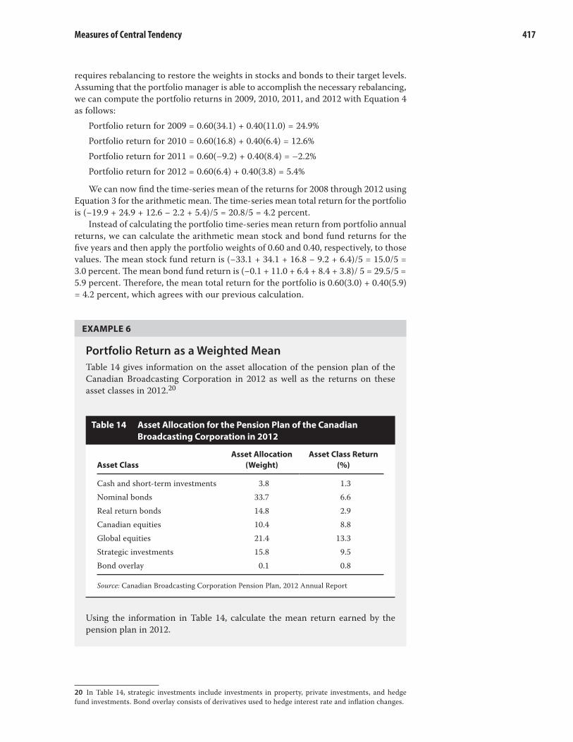
Measures of Central Tendency 417
requires rebalancing to restore the weights in stocks and bonds to their target levels.
Assuming that the portfolio manager is able to accomplish the necessary rebalancing,
we can compute the portfolio returns in 2009, 2010, 2011, and 2012 with Equation 4
as follows:
Portfolio return for 2009 = 0.60(34.1) + 0.40(11.0) = 24.9%
Portfolio return for 2010 = 0.60(16.8) + 0.40(6.4) = 12.6%
Portfolio return for 2011 = 0.60(–9.2) + 0.40(8.4) = –2.2%
Portfolio return for 2012 = 0.60(6.4) + 0.40(3.8) = 5.4%
We can now find the time- series mean of the returns for 2008 through 2012 using
Equation 3 for the arithmetic mean. The time- series mean total return for the portfolio
is (−19.9 + 24.9 + 12.6 − 2.2 + 5.4)/5 = 20.8/5 = 4.2 percent.
Instead of calculating the portfolio time- series mean return from portfolio annual
returns, we can calculate the arithmetic mean stock and bond fund returns for the
five years and then apply the portfolio weights of 0.60 and 0.40, respectively, to those
values. The mean stock fund return is (−33.1 + 34.1 + 16.8 − 9.2 + 6.4)/5 = 15.0/5 =
3.0 percent. The mean bond fund return is (−0.1 + 11.0 + 6.4 + 8.4 + 3.8)/ 5 = 29.5/5 =
5.9 percent. Therefore, the mean total return for the portfolio is 0.60(3.0) + 0.40(5.9)
= 4.2 percent, which agrees with our previous calculation.
EXAMPLE 6
Portfolio Return as a Weighted Mean
Table 14 gives information on the asset allocation of the pension plan of the
Canadian Broadcasting Corporation in 2012 as well as the returns on these
asset classes in 2012.20
Table 14 Asset Allocation for the Pension Plan of the Canadian
Broadcasting Corporation in 2012
Asset Class
Asset Allocation
(Weight)
Asset Class Return
(%)
Cash and short- term investments 3.8 1.3
Nominal bonds 33.7 6.6
Real return bonds 14.8 2.9
Canadian equities 10.4 8.8
Global equities 21.4 13.3
Strategic investments 15.8 9.5
Bond overlay 0.1 0.8
Source: Canadian Broadcasting Corporation Pension Plan, 2012 Annual Report
Using the information in Table 14, calculate the mean return earned by the
pension plan in 2012.
20 In Table 14, strategic investments include investments in property, private investments, and hedge
fund investments. Bond overlay consists of derivatives used to hedge interest rate and inflation changes.

Reading 8 ■ Statistical Concepts and Market Returns418
Solution:
Converting the percent asset allocation to decimal form, we find the mean return
as a weighted average of the asset class returns. We have
Mean portfolio return = 0.038(1.3%) + 0.337(6.6%) + 0.148(2.9%)
+ 0.104(8.8%) + 0.214(13.3%) + 0.158(9.5%)
+ 0.001(0.8%)
= 0.049% + 2.224% + 0.429% + 0.915% + 2.846%
+ 1.501% + 0.001%
= 8.0 percent
The previous examples illustrate the general principle that a portfolio return is a
weighted sum. Specifically, a portfolio’s return is the weighted average of the returns
on the assets in the portfolio; the weight applied to each asset’s return is the fraction
of the portfolio invested in that asset.
Market indexes are computed as weighted averages. For market- capitalization
indexes such as the CAC- 40 in France or the TOPIX in Japan or the S&P 500 in the
United States, each included stock receives a weight corresponding to its outstanding
market value divided by the total market value of all stocks in the index.
Our illustrations of weighted mean use past data, but they might just as well use
forward- looking data. When we take a weighted average of forward- looking data,
the weighted mean is called expected value. Suppose we make one forecast for the
year- end level of the S&P 500 assuming economic expansion and another forecast
for the year- end level of the S&P 500 assuming economic contraction. If we multiply
the first forecast by the probability of expansion and the second forecast by the prob-
ability of contraction and then add these weighted forecasts, we are calculating the
expected value of the S&P 500 at year- end. If we take a weighted average of possible
future returns on the S&P 500, we are computing the S&P 500’s expected return. The
probabilities must sum to 1, satisfying the condition on the weights in the expression
for weighted mean, Equation 4.
5.4.2 The Geometric Mean
The geometric mean is most frequently used to average rates of change over time
or to compute the growth rate of a variable. In investments, we frequently use the
geometric mean to average a time series of rates of return on an asset or a portfolio,
or to compute the growth rate of a financial variable such as earnings or sales. In
the reading on the time value of money, for instance, we computed a sales growth
rate (Example 17). That growth rate was a geometric mean. Because of the subject’s
importance, in a later section we will return to the use of the geometric mean and
offer practical perspectives on its use. The geometric mean is defined by the following
formula.
■ Geometric Mean Formula. The geometric mean, G, of a set of observations
X1, X2, …, Xn is
G X X X XX i n
nn
i
=
≥ =1 2 3
0 1 2with for , , , .
Equation 5 has a solution, and the geometric mean exists, only if the product under
the radical sign is non- negative. We impose the restriction that all the observations Xi
in Equation 5 are greater than or equal to zero. We can solve for the geometric mean
(5)

Measures of Central Tendency 419
using Equation 5 directly with any calculator that has an exponentiation key (on most
calculators, yx). We can also solve for the geometric mean using natural logarithms.
Equation 5 can also be stated as
ln ln Gn
X X X Xn= ( )11 2 3
or as
lnln
GX
n
ii
n
= =∑
1
When we have computed ln G, then G = elnG (on most calculators, the key for this
step is ex).
Risky assets can have negative returns up to −100 percent (if their price falls to zero),
so we must take some care in defining the relevant variables to average in computing
a geometric mean. We cannot just use the product of the returns for the sample and
then take the nth root because the returns for any period could be negative. We must
redefine the returns to make them positive. We do this by adding 1.0 to the returns
expressed as decimals. The term (1 + Rt) represents the year- ending value relative to
an initial unit of investment at the beginning of the year. As long as we use (1 + Rt), the
observations will never be negative because the biggest negative return is −100 percent.
The result is the geometric mean of 1 + Rt; by then subtracting 1.0 from this result,
we obtain the geometric mean of the individual returns Rt. For example, the returns
on RBC Canadian Index Fund during the 2008–2012 period were given in Table 13 as
−0.331, 0.341, 0.168, −0.092, and 0.064, putting the returns into decimal form. Adding
1.0 to those returns produces 0.669, 1.341, 1.168, 0.908, and 1.064. Using Equation 5
we have 0 669 1 341 1 168 0 908 1 0645 . . . . .( )( )( )( )( ) = 1 0123375 . = 1.002455.
This number is 1 plus the geometric mean rate of return. Subtracting 1.0 from
this result, we have 1.002455 − 1.0 = 0.002455 or approximately 0.25 percent. The
geometric mean return of RBC Canadian Index Fund during the 2008–2012 period
was 0.25 percent.
An equation that summarizes the calculation of the geometric mean return, RG,
is a slightly modified version of Equation 5 in which the Xi represent “1 + return in
decimal form.” Because geometric mean returns use time series, we use a subscript
t indexing time as well.
1 1 1 1
1 1
1 2
1
1
+ = +( ) +( ) +( )
+ = +( )⎡
⎣⎢⎢
⎤
⎦⎥⎥=
∏
R R R R
R R
G TT
G tt
T T
which leads to the following formula.
■ Geometric Mean Return Formula. Given a time series of holding period
returns Rt, t = 1, 2, …, T, the geometric mean return over the time period
spanned by the returns R1 through RT is
R RG tt
T T= +( )⎡
⎣⎢⎢
⎤
⎦⎥⎥
−=∏ 1 1
1
1
We can use Equation 6 to solve for the geometric mean return for any return data
series. Geometric mean returns are also referred to as compound returns. If the returns
being averaged in Equation 6 have a monthly frequency, for example, we may call the
(6)

Reading 8 ■ Statistical Concepts and Market Returns420
geometric mean monthly return the compound monthly return. The next example
illustrates the computation of the geometric mean while contrasting the geometric
and arithmetic means.
EXAMPLE 7
Geometric and Arithmetic Mean Returns (1)
As a mutual fund analyst, you are examining, as of early 2013, the most recent
five years of total returns for two US large- cap value equity mutual funds.
Table 15 Total Returns for Two Mutual Funds, 2008–2012
Year
Selected American Shares
(SLASX)
T. Rowe Price Equity Income
(PRFDX)
2008 −39.44% −35.75%
2009 31.64 25.62
2010 12.53 15.15
2011 −4.35 −0.72
2012 12.82 17.25
Source: performance.morningstar.com.
Based on the data in Table 15, address the following:
1 Calculate the geometric mean return of SLASX.
2 Calculate the arithmetic mean return of SLASX and contrast it to the
fund’s geometric mean return.
3 Calculate the geometric mean return of PRFDX.
4 Calculate the arithmetic mean return of PRFDX and contrast it to the
fund’s geometric mean return.
Solution to 1:
Converting the returns on SLASX to decimal form and adding 1.0 to each return
produces 0.6056, 1.3164, 1.1253, 0.9565, and 1.1282. We use Equation 6 to find
SLASX’s geometric mean return:
RG = ( )( )( )( )( ) −= −
0 6056 1 3164 1 1253 0 9565 1 1282 1
0 968084 1
5
5
. . . . .
. == − = −=
0 993534 1 0 006466. .−−0.65%
Solution to 2:
For SLASX, R = (−39.44 + 31.64 + 12.53 − 4.35 +12.82)/ 5 = 13.20/5 = 2.64%.
The arithmetic mean return for SLASX exceeds the geometric mean return by
2.64 − (−0.65) = 3.29% or 329 basis points.

Measures of Central Tendency 421
Solution to 3:
Converting the returns on PRFDX to decimal form and adding 1.0 to each return
produces 0.6425, 1.2562, 1.1515, 0.9928, and 1.1725. We use Equation 6 to find
PRFDX’s geometric mean return:
RG = ( )( )( )( )( ) −= −
0 6425 1 2562 1 1515 0 9928 1 1725 1
1 081859 1
5
5
. . . . .
. == − ==
1 015861 1 0 015861. .1.59%
Solution to 4:
PRFDX, R = (−35.75 + 25.62 + 15.15 − 0.72 + 17.25)/5 = 21.55/5 = 4.31%. The
arithmetic mean for PRFDX exceeds the geometric mean return by 4.31 − 1.59 =
2.72% or 272 basis points. The table below summarizes the findings.
Table 16 Mutual Fund Arithmetic and Geometric Mean
Returns: Summary of Findings
Fund Arithmetic Mean (%) Geometric Mean (%)
SLASX 2.64 −0.65
PRFDX 4.31 1.59
In Example 7, for both mutual funds, the geometric mean return was less than the
arithmetic mean return. In fact, the geometric mean is always less than or equal to
the arithmetic mean.21 The only time that the two means will be equal is when there
is no variability in the observations—that is, when all the observations in the series
are the same.22 In Example 7, there was variability in the funds’ returns; thus for both
funds, the geometric mean was strictly less than the arithmetic mean. In general,
the difference between the arithmetic and geometric means increases with the vari-
ability in the period- by- period observations.23 This relationship is also illustrated by
Example 7. Casual inspection suggests that the returns of SLASX are somewhat more
variable than those of PRFDX, and consequently, the spread between the arithmetic
and geometric mean returns is larger for SLASX (329 basis points) than for PRFDX
(272 basis points).24 Arithmetic and geometric returns need not always rank funds
similarly, however, in this example, PRFDX has both higher arithmetic and geometric
mean returns than SLASX. However, the difference between the geometric mean
returns of the two funds (2.24%) is greater than the difference between the arithmetic
mean returns of the two funds (1.67%). How should the analyst interpret these results?
21 This statement can be proved using Jensen’s inequality that the average value of a function is less than
or equal to the function evaluated at the mean if the function is concave from below—the case for ln(X).
22 For instance, suppose the return for each of the three years is 10 percent. The arithmetic mean is
10 percent. To find the geometric mean, we first express the returns as (1 + Rt) and then find the geometric
mean: [(1.10)(1.10)(1.10)]1/3 − 1.0 = 10 percent. The two means are the same.
23 We will soon introduce standard deviation as a measure of variability. Holding the arithmetic mean
return constant, the geometric mean return decreases for an increase in standard deviation.
24 We will introduce formal measures of variability later. But note, for example, the 71.08 percentage
point swing in returns between 2008 and 2009 for SLASX versus the 61.37 percentage point for PRFDX.
Similarly, note the 19.11 percentage point swing in returns between 2009 and 2010 for SLASX versus the
10.47 percentage point for PRFDX.

Reading 8 ■ Statistical Concepts and Market Returns422
The geometric mean return represents the growth rate or compound rate of return
on an investment. One dollar invested in SLASX at the beginning of 2008 would
have grown (or, in this case, decreased) to (0.6056)(1.3164)(1.1253)(0.9565)(1.1282)
= $0.9681, which is equal to 1 plus the geometric mean return compounded over five
periods: [1 + (−0.006466)]5 = (0.993534)5 = $0.9681, confirming that the geometric
mean is the compound rate of return. For PRFDX, one dollar would have grown to a
larger amount, (0.6425)(1.2562)(1.1515)(0.9928)(1.1725) = $1.0819, equal to (1.015861)5.
With its focus on the profitability of an investment over a multiperiod horizon, the
geometric mean is of key interest to investors. The arithmetic mean return, focusing on
average single- period performance, is also of interest. Both arithmetic and geometric
means have a role to play in investment management, and both are often reported for
return series. Example 8 highlights these points in a simple context.
EXAMPLE 8
Geometric and Arithmetic Mean Returns (2)
A hypothetical investment in a single stock initially costs €100. One year later,
the stock is trading at €200. At the end of the second year, the stock price falls
back to the original purchase price of €100. No dividends are paid during the
two- year period. Calculate the arithmetic and geometric mean annual returns.
Solution:
First, we need to find the Year 1 and Year 2 annual returns with Equation 1.
Return in Year 1 = 200/100 – 1 = 100%
Return in Year 2 = 100/200 – 1 = –50%
The arithmetic mean of the annual returns is (100% − 50%)/2 = 25%.
Before we find the geometric mean, we must convert the percentage rates
of return to (1 + Rt). After this adjustment, the geometric mean from Equation 6
is 2 0 0 50. . – 1 = 0 percent.
The geometric mean return of 0 percent accurately reflects that the ending
value of the investment in Year 2 equals the starting value in Year 1. The com-
pound rate of return on the investment is 0 percent. The arithmetic mean return
reflects the average of the one- year returns.
5.4.3 The Harmonic Mean
The arithmetic mean, the weighted mean, and the geometric mean are the most fre-
quently used concepts of mean in investments. A fourth concept, the harmonic
mean, X H , is appropriate in a limited number of applications.25
■ Harmonic Mean Formula. The harmonic mean of a set of observations X1, X2,
…, Xn is
X n X
X i n
H ii
n
i
= ( )
> ==∑ 1
0 1 21
with for , , ,
(7)
25 The terminology “harmonic” arises from its use relative to a type of series involving reciprocals known
as a harmonic series.

Other Measures of Location: Quantiles 423
The harmonic mean is the value obtained by summing the reciprocals of the observa-
tions—terms of the form 1/Xi—then averaging that sum by dividing it by the number
of observations n, and, finally, taking the reciprocal of the average.
The harmonic mean may be viewed as a special type of weighted mean in which an
observation’s weight is inversely proportional to its magnitude. The harmonic mean is
a relatively specialized concept of the mean that is appropriate when averaging ratios
(“amount per unit”) when the ratios are repeatedly applied to a fixed quantity to yield
a variable number of units. The concept is best explained through an illustration. A
well- known application arises in the investment strategy known as cost averaging,
which involves the periodic investment of a fixed amount of money. In this application,
the ratios we are averaging are prices per share at purchases dates, and we are apply-
ing those prices to a constant amount of money to yield a variable number of shares.
Suppose an investor purchases €1,000 of a security each month for n = 2 months.
The share prices are €10 and €15 at the two purchase dates. What is the average price
paid for the security?
In this example, in the first month we purchase €1,000/€10 = 100 shares and in the
second month we purchase €1,000/€15 = 66.67, or 166.67 shares in total. Dividing the
total euro amount invested, €2,000, by the total number of shares purchased, 166.67,
gives an average price paid of €2,000/166.67 = €12. The average price paid is in fact
the harmonic mean of the asset’s prices at the purchase dates. Using Equation 7,
the harmonic mean price is 2/[(1/10) + (1/15)] = €12. The value €12 is less than the
arithmetic mean purchase price (€10 + €15)/2 = €12.5. However, we could find the
correct value of €12 using the weighted mean formula, where the weights on the
purchase prices equal the shares purchased at a given price as a proportion of the
total shares purchased. In our example, the calculation would be (100/166.67)€10.00 +
(66.67/166.67)€15.00 = €12. If we had invested varying amounts of money at each
date, we could not use the harmonic mean formula. We could, however, still use the
weighted mean formula in a manner similar to that just described.
A mathematical fact concerning the harmonic, geometric, and arithmetic means is
that unless all the observations in a data set have the same value, the harmonic mean
is less than the geometric mean, which in turn is less than the arithmetic mean. In
the illustration given, the harmonic mean price was indeed less than the arithmetic
mean price.
OTHER MEASURES OF LOCATION: QUANTILES
Having discussed measures of central tendency, we now examine an approach to
describing the location of data that involves identifying values at or below which spec-
ified proportions of the data lie. For example, establishing that 25, 50, and 75 percent
of the annual returns on a portfolio are at or below the values −0.05, 0.16, and 0.25,
respectively, provides concise information about the distribution of portfolio returns.
Statisticians use the word quantile (or fractile) as the most general term for a value
at or below which a stated fraction of the data lies. In the following, we describe the
most commonly used quantiles—quartiles, quintiles, deciles, and percentiles—and
their application in investments.
6.1 Quartiles, Quintiles, Deciles, and Percentiles
We know that the median divides a distribution in half. We can define other dividing
lines that split the distribution into smaller sizes. Quartiles divide the distribution into
quarters, quintiles into fifths, deciles into tenths, and percentiles into hundredths.
6

Reading 8 ■ Statistical Concepts and Market Returns424
Given a set of observations, the yth percentile is the value at or below which y percent
of observations lie. Percentiles are used frequently, and the other measures can be
defined with respect to them. For example, the first quartile (Q1) divides a distribution
such that 25 percent of the observations lie at or below it; therefore, the first quartile
is also the 25th percentile. The second quartile (Q2) represents the 50th percentile,
and the third quartile (Q3) represents the 75th percentile because 75 percent of the
observations lie at or below it.
When dealing with actual data, we often find that we need to approximate the value
of a percentile. For example, if we are interested in the value of the 75th percentile, we
may find that no observation divides the sample such that exactly 75 percent of the
observations lie at or below that value. The following procedure, however, can help us
determine or estimate a percentile. The procedure involves first locating the position
of the percentile within the set of observations and then determining (or estimating)
the value associated with that position.
Let Py be the value at or below which y percent of the distribution lies, or the yth
percentile. (For example, P18 is the point at or below which 18 percent of the obser-
vations lie; 100 − 18 = 82 percent are greater than P18.) The formula for the position
of a percentile in an array with n entries sorted in ascending order is
L n yy = +( )1
100where y is the percentage point at which we are dividing the distribution and Ly is the
location (L) of the percentile (Py) in the array sorted in ascending order. The value of
Ly may or may not be a whole number. In general, as the sample size increases, the
percentile location calculation becomes more accurate; in small samples it may be
quite approximate.
As an example of the case in which Ly is not a whole number, suppose that we want
to determine the third quartile of returns for 2012 (Q3 or P75) for the 16 European
equity markets given in Table 8. According to Equation 8, the position of the third
quartile is L75 = (16 + 1)(75/100) = 12.75, or between the 12th and 13th items in Table 9,
which ordered the returns into ascending order. The 12th item in Table 9 is the return
to equities in France in 2012, 15.90 percent. The 13th item is the return to equities
in Austria in 2012, 20.72 percent. Reflecting the “0.75” in “12.75,” we would conclude
that P75 lies 75 percent of the distance between 15.90 percent and 20.72 percent.
To summarize:
■ When the location, Ly, is a whole number, the location corresponds to an actual
observation. For example, if Denmark had not been included in the sample,
then n + 1 would have been 16 and, with L75 = 12, the third quartile would be
P75 = X12, where Xi is defined as the value of the observation in the ith (i = L75)
position of the data sorted in ascending order (i.e., P75 =15.90).
■ When Ly is not a whole number or integer, Ly lies between the two closest
integer numbers (one above and one below), and we use linear interpolation
between those two places to determine Py. Interpolation means estimating an
unknown value on the basis of two known values that surround it (lie above
and below it); the term “linear” refers to a straight- line estimate. Returning
to the calculation of P75 for the equity returns, we found that Ly = 12.75; the
next lower whole number is 12 and the next higher whole number is 13. Using
linear interpolation, P75 ≈ X12 + (12.75 − 12) (X13 − X12). As above, in the
12th position is the return to equities in France, so X12 = 15.90 percent; X13 =
20.72 percent, the return to equities in Austria. Thus our estimate is P75 ≈ X12
+ (12.75 − 12)(X13 − X12) = 15.90 + 0.75 [20.72 − 15.90] = 15.90 + 0.75(4.82) =
15.90 + 3.62 = 19.52 percent. In words, 15.90 and 20.72 bracket P75 from below
and above, respectively. Because 12.75 − 12 = 0.75, using linear interpolation we
(8)

Other Measures of Location: Quantiles 425
move 75 percent of the distance from 15.90 to 20.72 as our estimate of P75. We
follow this pattern whenever Ly is a non- integer: The nearest whole numbers
below and above Ly establish the positions of observations that bracket Py and
then interpolate between the values of those two observations.
Example 9 illustrates the calculation of various quantiles for the dividend yield on the
components of a major European equity index.
EXAMPLE 9
Calculating Percentiles, Quartiles, and Quintiles
The EURO STOXX 50 is an index of 50 publicly traded companies, which pro-
vides a blue- chip representation of supersector leaders in the Eurozone. Table 17
shows the market capitalization on the 50 component stocks in the index, as
provided by STOXX Ltd. in September 2013. The market capitalizations are
ranked in ascending order.
Table 17 Market Capitalizations of the Components
of the EURO STOXX 50
No. Company Market Cap (Euro Billion)
1 Arcelor- Mittal 8.83
2 CRH 10.99
3 RWE 11.92
4 Carrefour 12.13
5 Repsol 12.84
6 Saint- Gobain 13.60
7 France Telecom 14.09
8 Unibail- Rodamco 15.96
9 Enel 16.33
10 Essilor International 16.85
11 Intesa Sanpaolo 17.00
12 Assicurazioni Generali 17.76
13 Vivendi 17.84
14 VINCI 18.64
15 Philips 19.04
16 EADS 19.37
17 Inditex 19.66
18 UniCredit 19.69
19 Iberdrola 20.29
20 BMW 20.69
21 ASML 20.71
22 Société Générale 20.92
23 GDF Suez 21.10
24 Volkswagen 21.57
25 Munich RE 22.25
26 E.ON 24.83
27 Deutsche Telekom 25.60
(continued)

Reading 8 ■ Statistical Concepts and Market Returns426
No. Company Market Cap (Euro Billion)
28 ING 25.93
29 Air Liquide 28.98
30 L’Oreal 29.20
31 Schneider Electric 29.75
32 AXA 30.13
33 Deutsche Bank 30.92
34 LVMH Moët Hennessy 32.36
35 Danone 33.36
36 BBVA 34.56
37 Telefonica 39.00
38 ENI 41.42
39 Daimler 42.42
40 BNP Paribas 43.09
41 Unilever 46.04
42 Allianz 47.72
43 Anheuser- Busch InBev 49.40
44 SAP 50.93
45 BCO Santander 51.17
46 BASF 63.88
47 Siemens 64.27
48 Bayer 65.83
49 Total 81.06
50 Sanofi 93.29
Source: www.stoxx.com accessed 27 September 2013.
Using the data in Table 17, address the following:
1 Calculate the 10th and 90th percentiles.
2 Calculate the first, second, and third quartiles.
3 State the value of the median.
4 How many quintiles are there, and to what percentiles do the quintiles
correspond?
5 Calculate the value of the first quintile.
Solution to 1:
In this example, n = 50. Using Equation 8, Ly = (n + 1)y/100 for position of the
yth percentile, so for the 10th percentile we have
L10 = (50 + 1)(10/100) = 5.1
L10 is between the fifth and sixth observations with values X5 = 12.84 and X6
= 13.60. The estimate of the 10th percentile (first decile) for dividend yield is
P10 ≈ X5 + (5.1 – 5)(X6 – X5) = 12.84 + 0.1(13.60 – 12.84)
= 12.84 + 0.1(0.76) = 12.92
Table 17 (Continued)

Other Measures of Location: Quantiles 427
For the 90th percentile,
L90 = (50 + 1)(90/100) = 45.9
L90 is between the 45th and 46th observations with values X45 = 51.17 and X46
= 63.88, respectively. The estimate of the 90th percentile (ninth decile) is
P90 ≈ X45 + (45.9 – 45)(X46 – X45) = 51.17 + 0.9(63.88 – 51.17)
= 51.17 + 0.9(12.71) = 62.61.
Solution to 2:
The first, second, and third quartiles correspond to P25, P50, and P75, respectively.
L25 = (51)(25/100) = 12.75 L25 is between the 12th and 13th entries
with values X12 = 17.76 and X13 = 17.84.
P25 = Q1 ≈ X12 + (12.75 – 12)(X13 – X12)
= 17.76 + 0.75(17.84 – 17.76)
= 17.76 + 0.75(0.08) = 17.82
L50 = (51)(50/100) = 25.5 L50 is between the 25th and 26th entries
with values, X25 = 22.25 and X26 = 24.83.
P50 = Q2 ≈ X25 + (25.50 – 25)(X26 – X25)
= 22.25 + 0.50(24.83 – 22.25)
= 22.25 + 0.50(2.58) = 23.54
L75 = (51)(75/100) = 38.25 L75 is between the 38th and 39th entries
with values X38 = 41.42 and X39 = 42.42.
P75 = Q3 ≈ X38 + (38.25 – 38)(X39 – X38)
= 41.42 + 0.25(42.42 – 41.42)
= 41.42 + 0.25(1.00) = 41.67
Solution to 3:
The median is the 50th percentile, 23.54. This is the same value that we would
obtain by taking the mean of the n/2 = 50/2 = 25th item and (n + 2)/2 = 52/2 =
26th items, consistent with the procedure given earlier for the median of an
even- numbered sample.
Solution to 4:
There are five quintiles, and they are specified by P20, P40, P60, and P80.
Solution to 5:
The first quintile is P20.
L20 = (50 + 1)(20/100) = 10.2 L20 is between the 10th and 11th observations
with values X10 = 16.85 and X11 = 17.00.
The estimate of the first quintile is
P20 ≈ X10 + (10.2 – 10)(X11 – X10) = 16.85 + 0.2(17.00 – 16.85)
= 16.85 + 0.2(0.15) = 16.88.
6.2 Quantiles in Investment Practice
In this section, we discuss the use of quantiles in investments. Quantiles are used in
portfolio performance evaluation as well as in investment strategy development and
research.

Reading 8 ■ Statistical Concepts and Market Returns428
Investment analysts use quantiles every day to rank performance—for example,
the performance of portfolios. The performance of investment managers is often
characterized in terms of the quartile in which they fall relative to the performance
of their peer group of managers. The Morningstar mutual fund star rankings, for
example, associates the number of stars with percentiles of performance relative to
similar- style mutual funds.
Another key use of quantiles is in investment research. Analysts refer to a group
defined by a particular quantile as that quantile. For example, analysts often refer to
the set of companies with returns falling below the 10th percentile cutoff point as
the bottom return decile. Dividing data into quantiles based on some characteristic
allows analysts to evaluate the impact of that characteristic on a quantity of inter-
est. For instance, empirical finance studies commonly rank companies based on the
market value of their equity and then sort them into deciles. The 1st decile contains
the portfolio of those companies with the smallest market values, and the 10th decile
contains those companies with the largest market value. Ranking companies by decile
allows analysts to compare the performance of small companies with large ones.
We can illustrate the use of quantiles, in particular quartiles, in investment research
using the example of Ibbotson et al. (2013). That study proposed an investment style
based on liquidity—buying stocks of less liquid stocks and selling stocks of more
liquid stocks. It compared the performance of this style with three already popular
investment styles, which include (1) firm size (buying stocks of small firms and selling
stocks of large firms), (2) value/growth (buying stocks of value firms, defined as firms
for which the stock price is relatively low in relation to earnings per share, book value
per share, or dividends per share, and selling stocks of growth firms, defined as firms
for which the stock price is relatively high in relation to those same measures), and
(3) momentum (buying stocks of firms with a high momentum in returns, or winners,
and selling stocks of firms with a low momentum, or losers.)
Ibbotson et al. examined the top 3,500 US stocks by market capitalization for the
period of 1971–2011. For each stock, they computed yearly measures of liquidity as
the annual share turnover (the sum of the 12 monthly volumes divided by each month’s
shares outstanding), size as the year- end market capitalization, value as the trailing
earnings- to- price ratio as of the year end, and momentum as the annual return. They
assigned one- fourth of the total sample with the lowest liquidity in a year to Quartile
1 and the one- fourth with the highest liquidity in that year to Quartile 4. The stocks
with the second- highest liquidity formed Quartile 3 and the stocks with the second-
lowest liquidity, Quartile 2. Treating each quartile group as a portfolio composed of
equally weighted stocks, they measured the returns on each liquidity quartile in the
following year (so that the quartiles are constructed “before the fact”.) The authors
repeated this process for each of the other three investment styles (size, value, and
momentum.) The results from Table 1 of their study are included in Table 18. We have
added a column with the spreads in returns from Quartile 1 to Quartile 4.
Table 18 reports each investment style’s geometric and arithmetic mean returns
and standard deviation of returns for each quartile grouping. In each style, moving
from Quartile 1 to Quartile 4, mean returns decrease. For example, the geometric
mean return for the least liquid stocks is 14.50% and for the most liquid stocks is
7.24%. Only for the case of size does standard deviation decrease at each step moving
from Quartile 1 to Quartile 4. Thus, the table provides evidence that the investment
styles generally having incremental value in explaining returns in relation to standard
deviation. The authors conclude that liquidity appears to differentiate the returns
approximately as well as the other styles.

Other Measures of Location: Quantiles 429
Table 18 Cross- Sectional Investment Style Returns (%) and Standard
Deviations of Returns (%), 1972–2011
Investment Style Q1 Q2 Q3 Q4
Spread
in Return,
Q1 to Q4
Size
(Q1 = micro; Q4 = large)
Geometric Mean 13.04 11.93 11.95 10.98 +2.06
Arithmetic Mean 16.42 14.69 14.14 12.61 +3.81
Standard deviation 27.29 24.60 21.82 18.35
Value
(Q1 = value; Q4 = growth)
Geometric Mean 16.13 13.60 10.10 7.62 +8.51
Arithmetic Mean 18.59 15.42 12.29 11.56 +7.03
Standard deviation 23.31 20.17 21.46 29.42
Momentum
(Q1 = winners; Q4 = losers)
Geometric Mean 12.85 14.25 13.26 7.18 +5.67
Arithmetic Mean 15.37 16.03 15.29 11.16 +4.21
Standard deviation 23.46 19.79 21.21 29.49
Liquidity
(Q1 = low; Q4 = high)
Geometric Mean 14.50 13.97 11.91 7.24 +7.26
Arithmetic Mean 16.38 16.05 14.39 11.04 +5.34
Standard deviation 20.41 21.50 23.20 28.48
Note: Each investment style portfolio contains as average of 742 stocks a year.
Source: Ibbotson et al.
To address the concern that liquidity may simply be a proxy for firm size, with
investing in less liquid firms being equivalent to investing in small firms, the authors
examined how less liquid stocks performed relative to more liquid stocks while con-
trolling for firm size. This step involved constructing equally- weighted double- sorted
portfolios in firm size and liquidity quartiles. That is, they constructed 16 different
liquidity and size portfolios (4 × 4 = 16) and investigated the interaction between
these two styles. The results from Table 2 of their article are included in Table 19.
We have added a column with the spreads in returns from Quartile 1 to Quartile 4
for each size category.
Table 19 Mean Annual Returns (%) and Standard Deviations of Returns (%) of Size and Liquidity Quartile
Portfolios, 1972–2011
Quartile
Q1
(Low liquidity) Q2 Q3
Q4
(High liquidity)
Spread
in Return,
Q1 to Q4
Microcap
Geometric Mean 15.36 16.21 9.94 1.32 +14.04
Arithmetic Mean 17.92 20.00 15.40 6.78 +11.14
(continued)

Reading 8 ■ Statistical Concepts and Market Returns430
Quartile
Q1
(Low liquidity) Q2 Q3
Q4
(High liquidity)
Spread
in Return,
Q1 to Q4
Standard deviation 23.77 29.41 35.34 34.20
Small cap
Geometric Mean 15.30 14.09 11.80 5.48 +9.82
Arithmetic Mean 17.07 16.82 15.38 9.89 +7.18
Standard deviation 20.15 24.63 28.22 31.21
Midcap
Geometric Mean 13.61 13.57 12.24 7.85 +5.76
Arithmetic Mean 15.01 15.34 14.51 11.66 +3.35
Standard deviation 17.91 20.10 22.41 28.71
Large cap
Geometric Mean 11.53 11.66 11.19 8.37 +3.16
Arithmetic Mean 12.83 12.86 12.81 11.58 +1.25
Standard deviation 16.68 15.99 18.34 25.75
Source: Ibbotson et al.
The table shows that within the quartile with the smallest firms, the low- liquidity
portfolio earned an annual geometric mean return of 15.36%, in contrast to the high-
liquidity portfolio return of 1.32%, producing a liquidity effect of 14.04 percentage
points (1,404 basis points). While the liquidity effect is strongest for the smallest firms,
it does persist in other three size quartiles also. These results indicate that size does
not capture liquidity (i.e., the liquidity effect holds regardless of size group).
MEASURES OF DISPERSION
As the well- known researcher Fischer Black has written, “[t]he key issue in investments
is estimating expected return.”26 Few would disagree with the importance of expected
return or mean return in investments: The mean return tells us where returns, and
investment results, are centered. To completely understand an investment, however,
we also need to know how returns are dispersed around the mean. Dispersion is the
variability around the central tendency. If mean return addresses reward, dispersion
addresses risk.
In this section, we examine the most common measures of dispersion: range,
mean absolute deviation, variance, and standard deviation. These are all measures of
absolute dispersion. Absolute dispersion is the amount of variability present without
comparison to any reference point or benchmark.
These measures are used throughout investment practice. The variance or standard
deviation of return is often used as a measure of risk pioneered by Nobel laureate
Harry Markowitz. William Sharpe, another winner of the Nobel Prize in economics,
7
Table 19 (Continued)
26 Black (1993).

Measures of Dispersion 431
developed the Sharpe ratio, a measure of risk- adjusted performance. That measure
makes use of standard deviation of return. Other measures of dispersion, mean abso-
lute deviation and range, are also useful in analyzing data.
7.1 The Range
We encountered range earlier when we discussed the construction of frequency
distribution. The simplest of all the measures of dispersion, range can be computed
with interval or ratio data.
■ Definition of Range. The range is the difference between the maximum and
minimum values in a data set:
Range = Maximum value – Minimum value
As an illustration of range, the largest monthly return for the S&P 500 in the period
from January 1926 to December 2012 is 42.56 percent (in April 1933) and the small-
est is −29.73 percent (in September 1931). The range of returns is thus 72.29 percent
[42.56 percent − (−29.73 percent)]. An alternative definition of range reports the
maximum and minimum values. This alternative definition provides more information
than does the range as defined in Equation 9.
One advantage of the range is ease of computation. A disadvantage is that the
range uses only two pieces of information from the distribution. It cannot tell us how
the data are distributed (that is, the shape of the distribution). Because the range is
the difference between the maximum and minimum returns, it can reflect extremely
large or small outcomes that may not be representative of the distribution.27
7.2 The Mean Absolute Deviation
Measures of dispersion can be computed using all the observations in the distribution
rather than just the highest and lowest. The question is, how should we measure
dispersion? Our previous discussion on properties of the arithmetic mean introduced
the notion of distance or deviation from the mean X Xi −( ) as a fundamental piece
of information used in statistics. We could compute measures of dispersion as the
arithmetic average of the deviations around the mean, but we would encounter a
problem: The deviations around the mean always sum to 0. If we computed the mean
of the deviations, the result would also equal 0. Therefore, we need to find a way to
address the problem of negative deviations canceling out positive deviations.
One solution is to examine the absolute deviations around the mean as in the
mean absolute deviation.
■ Mean Absolute Deviation Formula. The mean absolute deviation (MAD) for
a sample is
MAD =
−=∑ X X
n
ii
n
1
where X is the sample mean and n is the number of observations in the sample.
(9)
(10)
27 Another distance measure of dispersion that we may encounter, the interquartile range, focuses on the
middle rather than the extremes. The interquartile range (IQR) is the difference between the third and
first quartiles of a data set: IQR = Q3 − Q1. The IQR represents the length of the interval containing the
middle 50 percent of the data, with a larger interquartile range indicating greater dispersion, all else equal.

Reading 8 ■ Statistical Concepts and Market Returns432
In calculating MAD, we ignore the signs of the deviations around the mean. For
example, if Xi = −11.0 and X = 4.5, the absolute value of the difference is |−11.0 − 4.5|
= |−15.5| = 15.5. The mean absolute deviation uses all of the observations in the sample
and is thus superior to the range as a measure of dispersion. One technical drawback
of MAD is that it is difficult to manipulate mathematically compared with the next
measure we will introduce, variance.28 Example 10 illustrates the use of the range and
the mean absolute deviation in evaluating risk.
EXAMPLE 10
The Range and the Mean Absolute Deviation
Having calculated mean returns for the two mutual funds in Example 7, the
analyst is now concerned with evaluating risk.
Table 15 Total Returns for Two Mutual Funds, 2008–2012 (Repeated)
Year
Selected American Shares
(SLASX)
T. Rowe Price Equity Income
(PRFDX)
2008 −39.44% −35.75%
2009 31.64 25.62
2010 12.53 15.15
2011 −4.35 −0.72
2012 12.82 17.25
Source: performance.morningstar.com.
Based on the data in Table 15 on the previous page, answer the following:
1 Calculate the range of annual returns for (A) SLASX and (B) PRFDX, and
state which mutual fund appears to be riskier based on these ranges.
2 Calculate the mean absolute deviation of returns on (A) SLASX and
(B) PRFDX, and state which mutual fund appears to be riskier based on
MAD.
Solution to 1:
A For SLASX, the largest return was 31.64 percent and the smallest was
−39.44 percent. The range is thus 31.64 − (−39.44) = 71.08%.
B For PFRDX, the range is 25.62 − (−35.75) = 61.37%. With a larger range of
returns than PRFDX, SLASX appeared to be the riskier fund during the
2008–2012 period.
28 In some analytic work such as optimization, the calculus operation of differentiation is important.
Variance as a function can be differentiated, but absolute value cannot.

Measures of Dispersion 433
Solution to 2:
A The arithmetic mean return for SLASX as calculated in Example 7 is
2.64 percent. The MAD of SLASX returns is
MAD
=− − + − + − + − − + −39 44 2 64 31 64 2 64 12 53 2 64 4 35 2 64 12 82 2 6. . . . . . . . . . 44
542 08 29 00 9 89 6 99 10 18
598 14
519 63
=+ + + +
= =
. . . . .
. . %
B The arithmetic mean return for PRFDX as calculated in Example 7 is
4.31 percent. The MAD of PRFDX returns is
MAD
=− − + − + − + − − + −35 75 4 31 25 62 4 31 15 15 4 31 0 72 4 31 17 25 4 3. . . . . . . . . . 11
540 06 21 31 10 84 5 03 12 94
590 18
518 04
=+ + + +
= =
. . . . .
. . %
SLASX, with a MAD of 19.63 percent, appears to be slightly riskier than PRFDX,
with a MAD of 18.04 percent.
7.3 Population Variance and Population Standard Deviation
The mean absolute deviation addressed the issue that the sum of deviations from the
mean equals zero by taking the absolute value of the deviations. A second approach
to the treatment of deviations is to square them. The variance and standard deviation,
which are based on squared deviations, are the two most widely used measures of
dispersion. Variance is defined as the average of the squared deviations around the
mean. Standard deviation is the positive square root of the variance. The following
discussion addresses the calculation and use of variance and standard deviation.
7.3.1 Population Variance
If we know every member of a population, we can compute the population variance.
Denoted by the symbol σ2, the population variance is the arithmetic average of the
squared deviations around the mean.
■ Population Variance Formula. The population variance is
σ
μ2 =
−( )=∑ X
N
ii
N 2
1
where μ is the population mean and N is the size of the population.
Given knowledge of the population mean, μ, we can use Equation 11 to calculate the
sum of the squared differences from the mean, taking account of all N items in the
population, and then to find the mean squared difference by dividing the sum by N.
Whether a difference from the mean is positive or negative, squaring that difference
results in a positive number. Thus variance takes care of the problem of negative devi-
ations from the mean canceling out positive deviations by the operation of squaring
those deviations. The profit as a percentage of revenue for BJ’s Wholesale Club, Costco,
(11)

Reading 8 ■ Statistical Concepts and Market Returns434
and Walmart was given earlier as 0.9, 1.6, and 3.5, respectively. We calculated the
mean profit as a percentage of revenue as 2.0. Therefore, the population variance of
the profit as a percentage of revenue is (1/3)[(0.9 − 2.0)2 + (1.6 − 2.0)2 + (3.5 − 2.0)2]
= (1/3)(−1.12 + −0.42 + 1.52) = (1/3)(1.21 + 0.16 + 2.25) = (1/3)(3.62) = 1.21.
7.3.2 Population Standard Deviation
Because the variance is measured in squared units, we need a way to return to the
original units. We can solve this problem by using standard deviation, the square root
of the variance. Standard deviation is more easily interpreted than the variance because
standard deviation is expressed in the same unit of measurement as the observations.
■ Population Standard Deviation Formula. The population standard devia-
tion, defined as the positive square root of the population variance, is
σ
μ
=
−( )=∑ X
N
ii
N 2
1
where μ is the population mean and N is the size of the population.
Using the example of the profit as a percentage of revenue for BJ’s Wholesale Club,
Costco, and Walmart, according to Equation 12 we would calculate the variance, 1.21,
then take the square root: 1 21. = 1.10.
Both the population variance and standard deviation are examples of parameters of
a distribution. In later readings, we will introduce the notion of variance and standard
deviation as risk measures.
In investments, we often do not know the mean of a population of interest, usually
because we cannot practically identify or take measurements from each member of
the population. We then estimate the population mean with the mean from a sample
drawn from the population, and we calculate a sample variance or standard deviation
using formulas different from Equations 11 and 12. We shall discuss these calcula-
tions in subsequent sections. However, in investments we sometimes have a defined
group that we can consider to be a population. With well- defined populations, we use
Equations 11 and 12, as in the following example.
EXAMPLE 11
Calculating the Population Standard Deviation
Table 20 gives the yearly portfolio turnover for the 12 US equity funds that com-
posed the 2013 Forbes Magazine Honor Roll.29 Portfolio turnover, a measure of
trading activity, is the lesser of the value of sales or purchases over a year divided
by average net assets during the year. The number and identity of the funds on
the Forbes Honor Roll changes from year to year.
(12)
29 Forbes magazine annually selects US equity mutual funds meeting certain criteria for its Honor Roll.
The criteria relate to capital preservation (performance in bear markets), continuity of management (the
fund must have a manager with at least six years’ tenure), diversification, accessibility (disqualifying funds
that are closed to new investors), and after- tax long- term performance.

Measures of Dispersion 435
Table 20 Portfolio Turnover: 2013 Forbes Honor Roll Mutual Funds
Fund
Yearly Portfolio
Turnover (%)
Bruce Fund (BRUFX) 10
CGM Focus Fund (CGMFX) 360
Hotchkis And Wiley Small Cap Value A Fund
(HWSAX)37
Aegis Value Fund (AVALX) 20
Delafield Fund (DEFIX) 49
Homestead Small Company Stock Fund (HSCSX) 1
Robeco Boston Partners Small Cap Value II Fund
(BPSCX)32
Hotchkis And Wiley Mid Cap Value A Fund
(HWMAX)72
T Rowe Price Small Cap Value Fund (PRSVX) 9
Guggenheim Mid Cap Value Fund Class A (SEVAX) 19
Wells Fargo Advantage Small Cap Value Fund
(SSMVX)16
Stratton Small- Cap Value Fund (STSCX) 11
Source: Forbes (2013).
Based on the data in Table 20, address the following:
1 Calculate the population mean portfolio turnover for the period used by
Forbes for the 12 Honor Roll funds.
2 Calculate the population variance and population standard deviation of
portfolio turnover.
3 Explain the use of the population formulas in this example.
Solution to 1:
μ = (10 + 360 + 37 + 20 + 49 + 1 + 32 + 72 + 9 + 19 + 16 + 11)/12
= 636 /12 = 53 percent.
Solution to 2:
Having established that μ = 53, we can calculate σ
μ2
2
1=
−( )=∑ X
N
ii
N
by first
calculating the numerator in the expression and then dividing by N = 12. The
numerator (the sum of the squared differences from the mean) is
(10 – 53)2 + (360 – 53)2 + (37 – 53)2 + (20 – 53)2 + (49 – 53)2 + (1 – 53)2 + (32 – 53)2 + (72 – 53)2 + (9 – 53)2 + (19 – 53)2 + (16 – 53)2 + (11 – 53)2 = 107,190
Thus σ2 = 107,190/12 = 8,932.50.
To calculate standard deviation, σ = 8 932 50, . = 94.51 percent. (The unit
of variance is percent squared so the unit of standard deviation is percent.)

Reading 8 ■ Statistical Concepts and Market Returns436
Solution to 3:
If the population is clearly defined to be the Forbes Honor Roll funds in one
specific year (2013), and if portfolio turnover is understood to refer to the specific
one- year period reported upon by Forbes, the application of the population for-
mulas to variance and standard deviation is appropriate. The results of 8,932.50
and 94.51 are, respectively, the cross- sectional variance and standard deviation
in yearly portfolio turnover for the 2013 Forbes Honor Roll Funds.30
7.4 Sample Variance and Sample Standard Deviation
In the following discussion, note the switch to Roman letters to symbolize sample
quantities.
7.4.1 Sample Variance
In many instances in investment management, a subset or sample of the population
is all that we can observe. When we deal with samples, the summary measures are
called statistics. The statistic that measures the dispersion in a sample is called the
sample variance.
■ Sample Variance Formula. The sample variance is
sX X
n
ii
n
2
2
11
=
−( )−
=∑
where X is the sample mean and n is the number of observations in the sample.
Equation 13 tells us to take the following steps to compute the sample variance:
i. Calculate the sample mean, X .
ii. Calculate each observation’s squared deviation from the sample
mean, X Xi −( )2 .
iii. Sum the squared deviations from the mean: X Xii
n−( )
=∑ 2
1.
iv. Divide the sum of squared deviations from the mean by
n – 1: X X nii
n−( ) −( )
=∑ 2
11 .
We will illustrate the calculation of the sample variance and the sample standard
deviation in Example 12.
We use the notation s2 for the sample variance to distinguish it from population
variance, σ2. The formula for sample variance is nearly the same as that for population
variance except for the use of the sample mean, X , in place of the population mean,
μ, and a different divisor. In the case of the population variance, we divide by the size
of the population, N. For the sample variance, however, we divide by the sample size
minus 1, or n − 1. By using n − 1 (rather than n) as the divisor, we improve the sta-
tistical properties of the sample variance. In statistical terms, the sample variance
defined in Equation 13 is an unbiased estimator of the population variance.31 The
(13)
30 In fact, we could not properly use the Honor Roll funds to estimate the population variance of portfolio
turnover (for example) of any other differently defined population, because the Honor Roll funds are not
a random sample from any larger population of US equity mutual funds.
31 We discuss this concept further in the reading on sampling.
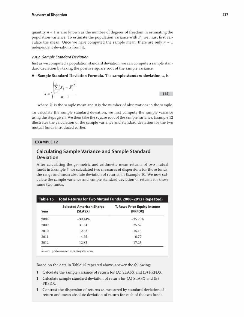
Measures of Dispersion 437
quantity n − 1 is also known as the number of degrees of freedom in estimating the
population variance. To estimate the population variance with s2, we must first cal-
culate the mean. Once we have computed the sample mean, there are only n − 1
independent deviations from it.
7.4.2 Sample Standard Deviation
Just as we computed a population standard deviation, we can compute a sample stan-
dard deviation by taking the positive square root of the sample variance.
■ Sample Standard Deviation Formula. The sample standard deviation, s, is
sX X
n
ii
n
=
−( )−
=∑ 2
11
where X is the sample mean and n is the number of observations in the sample.
To calculate the sample standard deviation, we first compute the sample variance
using the steps given. We then take the square root of the sample variance. Example 12
illustrates the calculation of the sample variance and standard deviation for the two
mutual funds introduced earlier.
EXAMPLE 12
Calculating Sample Variance and Sample Standard
Deviation
After calculating the geometric and arithmetic mean returns of two mutual
funds in Example 7, we calculated two measures of dispersions for those funds,
the range and mean absolute deviation of returns, in Example 10. We now cal-
culate the sample variance and sample standard deviation of returns for those
same two funds.
Table 15 Total Returns for Two Mutual Funds, 2008–2012 (Repeated)
Year
Selected American Shares
(SLASX)
T. Rowe Price Equity Income
(PRFDX)
2008 −39.44% −35.75%
2009 31.64 25.62
2010 12.53 15.15
2011 −4.35 −0.72
2012 12.82 17.25
Source: performance.morningstar.com.
Based on the data in Table 15 repeated above, answer the following:
1 Calculate the sample variance of return for (A) SLASX and (B) PRFDX.
2 Calculate sample standard deviation of return for (A) SLASX and (B)
PRFDX.
3 Contrast the dispersion of returns as measured by standard deviation of
return and mean absolute deviation of return for each of the two funds.
(14)

Reading 8 ■ Statistical Concepts and Market Returns438
Solution to 1:
To calculate the sample variance, we use Equation 13. (Deviation answers are
all given in percent squared.)
A SLASX
i. The sample mean is
R = (−39.44 + 31.64 + 12.53 − 4.35 +12.82)/ 5 = 13.20/5 = 2.64%.
ii. The squared deviations from the mean are
(–39.44 – 2.64)2 = (–42.08)2 = 1,770.73
(31.64 – 2.64)2 = (29.00)2 = 841.00
(12.53 – 2.64)2 = (9.89)2 = 97.81
(–4.35 – 2.64)2 = (–6.99)2 = 48.86
(12.82 – 2.64)2 = (10.18)2 = 103.63
iii. The sum of the squared deviations from the mean is 1,770.73 +
841.00 + 97.81 + 48.86 + 103.63 = 2,862.03.
iv. Divide the sum of the squared deviations from the mean by n − 1:
2,862.03/(5 − 1) = 2,862.03/4 = 715.51
B PRFDX
i. The sample mean is
R = (−35.75 + 25.62 + 15.15 − 0.72 + 17.25)/5 = 21.55/5 = 4.31%.
ii. The squared deviations from the mean are
(–35.75 – 4.31)2 = (–40.06)2 = 1,604.80
(25.62 – 4.31)2 = (21.31)2 = 454.12
(15.15 – 4.31)2 = (10.84)2 = 117.51
(–0.72 – 4.31)2 = (–5.03)2 = 25.30
(17.25 – 4.31)2 = (12.94)2 = 167.44
iii. The sum of the squared deviations from the mean is 1,604.80 +
454.12 + 117.51 + 25.30 + 167.44 = 2,369.17.
iv. Divide the sum of the squared deviations from the mean by n − 1:
2,369.17/4 = 592.29
Solution to 2:
To find the standard deviation, we take the positive square root of variance.
A For SLASX, s 715 51. = 26.7%.
B For PRFDX, s 592 29. = 24.3%.
Solution to 3:
Table 21 summarizes the results from Part 2 for standard deviation and incor-
porates the results for MAD from Example 10.

Measures of Dispersion 439
Table 21 Two Mutual Funds: Comparison of Standard Deviation and
Mean Absolute Deviation
Fund Standard Deviation (%) Mean Absolute Deviation (%)
SLASX 26.7 19.6
PRFDX 24.3 18.0
Note that the mean absolute deviation is less than the standard deviation.
The mean absolute deviation will always be less than or equal to the standard
deviation because the standard deviation gives more weight to large deviations
than to small ones (remember, the deviations are squared).
Because the standard deviation is a measure of dispersion about the arithmetic
mean, we usually present the arithmetic mean and standard deviation together when
summarizing data. When we are dealing with data that represent a time series of
percent changes, presenting the geometric mean—representing the compound rate of
growth—is also very helpful. Table 22 presents the historical geometric and arithmetic
mean returns, along with the historical standard deviation of returns, for the S&P 500
annual and monthly return series. We present these statistics for nominal (rather than
inflation- adjusted) returns so we can observe the original magnitudes of the returns.
Table 22 Equity Market Returns: Means and Standard Deviations
Return Series
Geometric
Mean (%)
Arithmetic
Mean (%)
Standard
Deviation
Ibbotson Associates Series: 1926–2012
S&P 500 (Annual) 9.84 11.82 20.18
S&P 500 (Monthly) 0.79 0.94 5.50
Source: Ibbotson.
7.5 Semivariance, Semideviation, and Related Concepts
An asset’s variance or standard deviation of returns is often interpreted as a measure of
the asset’s risk. Variance and standard deviation of returns take account of returns above
and below the mean, but investors are concerned only with downside risk, for example,
returns below the mean. As a result, analysts have developed semivariance, semidevi-
ation, and related dispersion measures that focus on downside risk. Semivariance is
defined as the average squared deviation below the mean. Semideviation (sometimes
called semistandard deviation) is the positive square root of semivariance.32 To com-
pute the sample semivariance, for example, we take the following steps:
i. Calculate the sample mean.
ii. Identify the observations that are smaller than or equal to the mean (discarding
observations greater than the mean).
32 This is an informal treatment of these two measures; see the survey article by N. Fred Choobinbeh
(2005) for a rigorous treatment.

Reading 8 ■ Statistical Concepts and Market Returns440
iii. Compute the sum of the squared negative deviations from the mean (using the
observations that are smaller than or equal to the mean).
iv. Divide the sum of the squared negative deviations from Step iii by the total
sample size minus 1: n − 1. A formula for semivariance approximating the unbi-
ased estimator is
X X niX Xi
−( ) −( )≤
∑ 2 1for all
To take the case of Selected American Shares with returns (in percent) of −39.44,
31.64, 12.53, −4.35, and 12.82, we earlier calculated a mean return of 2.64 percent.
Two returns, −39.44 and −4.35, are smaller than 2.64. We compute the sum of the
squared negative deviations from the mean as (−39.44 − 2.64)2 + (−4.35 − 2.64)2 =
−42.082 + −6.992 = 1,770.73 + 48.86 = 1,819.59. With n − 1 = 4, we conclude that
semivariance is 1,819.59/4 = 454.9 and that semideviation is 454 9. = 21.3 percent,
approximately. The semideviation of 21.3 percent is less than the standard deviation
of 26.7 percent. From this downside risk perspective, therefore, standard deviation
overstates risk.
In practice, we may be concerned with values of return (or another variable) below
some level other than the mean. For example, if our return objective is 12.75 percent
annually, we may be concerned particularly with returns below 12.75 percent a year.
We can call 12.75 percent the target. The name target semivariance has been given
to average squared deviation below a stated target, and target semideviation is its
positive square root. To calculate a sample target semivariance, we specify the target
as a first step. After identifying observations below the target, we find the sum of the
squared negative deviations from the target and divide that sum by the number of
observations minus 1. A formula for target semivariance is
X B niX Bi
−( ) −( )≤
∑ 2 1for all
where B is the target and n is the number of observations. With a target return of
12.75 percent, we find in the case of Selected American Shares that three returns
(−39.44, 12.53, and −4.35) were below the target. The target semivariance is [(−39.44
− 12.75)2 + (12.53 − 12.75)2 + (−4.35 − 12.75)2]/(5 – 1) = 754.06, and the target
semideviation is 754 06. = 27.5 percent, approximately.
When return distributions are symmetric, semivariance and variance are effectively
equivalent. For asymmetric distributions, variance and semivariance rank prospects’
risk differently.33 Semivariance (or semideviation) and target semivariance (or target
semideviation) have intuitive appeal, but they are harder to work with mathematically
than variance.34 Variance or standard deviation enters into the definition of many of
the most commonly used finance risk concepts, such as the Sharpe ratio and beta.
Perhaps because of these reasons, variance (or standard deviation) is much more
frequently used in investment practice.
33 See Estrada (2003). We discuss skewness later in this reading.
34 As discussed in the reading on probability concepts and the various readings on portfolio concepts,
we can find a portfolio’s variance as a straightforward function of the variances and correlations of the
component securities. There is no similar procedure for semivariance and target semivariance. We also
cannot take the derivative of semivariance or target semivariance.

Measures of Dispersion 441
7.6 Chebyshev’s Inequality
The Russian mathematician Pafnuty Chebyshev developed an inequality using standard
deviation as a measure of dispersion. The inequality gives the proportion of values
within k standard deviations of the mean.
■ Definition of Chebyshev’s Inequality. According to Chebyshev’s inequality, for
any distribution with finite variance, the proportion of the observations within
k standard deviations of the arithmetic mean is at least 1 − 1/k2 for all k > 1.
Table 23 illustrates the proportion of the observations that must lie within a certain
number of standard deviations around the sample mean.
Table 23 Proportions from Chebyshev’s Inequality
k Interval around the Sample Mean Proportion (%)
1.25 X s125. 36
1.50 X s15. 0 56
2.00 X s2 75
2.50 X s2 5. 0 84
3.00 X s3 89
4.00 X s4 94
Note: Standard deviation is denoted as s.
When k = 1.25, for example, the inequality states that the minimum proportion of the
observations that lie within ± 1.25s is 1 − 1/(1.25)2 = 1 − 0.64 = 0.36 or 36 percent.
The most frequently cited facts that result from Chebyshev’s inequality are that
a two- standard- deviation interval around the mean must contain at least 75 percent
of the observations, and a three- standard- deviation interval around the mean must
contain at least 89 percent of the observations, no matter how the data are distributed.
The importance of Chebyshev’s inequality stems from its generality. The inequality
holds for samples and populations and for discrete and continuous data regardless of
the shape of the distribution. As we shall see in the reading on sampling, we can make
much more precise interval statements if we can assume that the sample is drawn
from a population that follows a specific distribution called the normal distribution.
Frequently, however, we cannot confidently assume that distribution.
The next example illustrates the use of Chebyshev’s inequality.

Reading 8 ■ Statistical Concepts and Market Returns442
EXAMPLE 13
Applying Chebyshev’s Inequality
According to Table 22, the arithmetic mean monthly return and standard devi-
ation of monthly returns on the S&P 500 were 0.94 percent and 5.50 percent,
respectively, during the 1926–2012 period, totaling 1,044 monthly observations.
Using this information, address the following:
1 Calculate the endpoints of the interval that must contain at least 75 per-
cent of monthly returns according to Chebyshev’s inequality.
2 What are the minimum and maximum number of observations that
must lie in the interval computed in Part 1, according to Chebyshev’s
inequality?
Solution to 1:
According to Chebyshev’s inequality, at least 75 percent of the observations
must lie within two standard deviations of the mean, X ± 2s. For the monthly
S&P 500 return series, we have 0.94% ± 2(5.50%) = 0.94% ± 11.00%. Thus the
lower endpoint of the interval that must contain at least 75 percent of the
observations is 0.94% − 11.00% = −10.06%, and the upper endpoint is 0.94% +
11.00% = 11.94%.
Solution to 2:
For a sample size of 1,044, at least 0.75(1,044) = 783 observations must lie in
the interval from −10.06% to 11.94% that we computed in Part 1. Chebyshev’s
inequality gives the minimum percentage of observations that must fall within a
given interval around the mean, but it does not give the maximum percentage.
Table 4, which gave the frequency distribution of monthly returns on the S&P
500, is excerpted below. The data in the excerpted table are consistent with the
prediction of Chebyshev’s inequality. The set of intervals running from −10.0% to
12.0% is about equal in width to the two- standard- deviation interval −10.06% to
11.94%. A total of 1,004 observations (approximately 96 percent of observations)
fall in the range from −10.0% to 12.0%.
Table 4 Frequency Distribution for the Monthly Total
Return on the S&P 500, January 1926 to
December 2012 (Excerpt)
Return Interval (%) Absolute Frequency
−10.0 to −8.0 23
−8.0 to −6.0 34
−6.0 to −4.0 59
−4.0 to −2.0 98
−2.0 to 0.0 157
0.0 to 2.0 220
2.0 to 4.0 173
4.0 to 6.0 137
6.0 to 8.0 63
8.0 to 10.0 25

Measures of Dispersion 443
Return Interval (%) Absolute Frequency
10.0 to 12.0 15
1,004
7.7 Coefficient of Variation
We noted earlier that standard deviation is more easily interpreted than variance
because standard deviation uses the same units of measurement as the observations.
We may sometimes find it difficult to interpret what standard deviation means in terms
of the relative degree of variability of different sets of data, however, either because
the data sets have markedly different means or because the data sets have different
units of measurement. In this section we explain a measure of relative dispersion, the
coefficient of variation that can be useful in such situations. Relative dispersion is
the amount of dispersion relative to a reference value or benchmark.
We can illustrate the problem of interpreting the standard deviation of data sets
with markedly different means using two hypothetical samples of companies. The
first sample, composed of small companies, includes companies with 2003 sales of
€50 million, €75 million, €65 million, and €90 million. The second sample, composed
of large companies, includes companies with 2003 sales of €800 million, €825 million,
€815 million, and €840 million. We can verify using Equation 14 that the standard
deviation of sales in both samples is €16.8 million.35 In the first sample, the largest
observation, €90 million, is 80 percent larger than the smallest observation, €50 mil-
lion. In the second sample, the largest observation is only 5 percent larger than the
smallest observation. Informally, a standard deviation of €16.8 million represents a
high degree of variability relative to the first sample, which reflects mean 2003 sales
of €70 million, but a small degree of variability relative to the second sample, which
reflects mean 2003 sales of €820 million.
The coefficient of variation is helpful in situations such as that just described.
■ Coefficient of Variation Formula. The coefficient of variation, CV, is the ratio
of the standard deviation of a set of observations to their mean value:36
CV s X
where s is the sample standard deviation and X is the sample mean.
When the observations are returns, for example, the coefficient of variation measures
the amount of risk (standard deviation) per unit of mean return. Expressing the mag-
nitude of variation among observations relative to their average size, the coefficient of
variation permits direct comparisons of dispersion across different data sets. Reflecting
the correction for scale, the coefficient of variation is a scale- free measure (that is, it
has no units of measurement).
We can illustrate the application of the coefficient of variation using our earlier
example of two samples of companies. The coefficient of variation for the first sam-
ple is (€16.8 million)/(€70 million) = 0.24; the coefficient of variation for the second
(15)
Table 4 (Continued)
35 The second sample was created by adding €750 million to each observation in the first sample. Standard
deviation (and variance) has the property of remaining unchanged if we add a constant amount to each
observation.
36 The reader will also encounter CV defined as 100(s/ X ), which states CV as a percentage.

Reading 8 ■ Statistical Concepts and Market Returns444
sample is (€16.8 million)/(€820 million) = 0.02. This confirms our intuition that the
first sample had much greater variability in sales than the second sample. Note that
0.24 and 0.02 are pure numbers in the sense that they are free of units of measurement
(because we divided the standard deviation by the mean, which is measured in the
same units as the standard deviation). If we need to compare the dispersion among
data sets stated in different units of measurement, the coefficient of variation can
be useful because it is free from units of measurement. Example 14 illustrates the
calculation of the coefficient of variation.
EXAMPLE 14
Calculating the Coefficient of Variation
Table 24 summarizes annual mean returns and standard deviations computed
using monthly return data for major stock market indexes of four Asia- Pacific
markets. The indexes are: S&P/ASX 200 Index (Australia), Hang Seng Index
(Hong Kong), Straits Times Index (Singapore), and KOSPI Composite Index
(South Korea).
Table 24 Arithmetic Mean Annual Return and Standard Deviation of
Returns, Asia- Pacific Stock Markets, 2003–2012
Market
Arithmetic Mean
Return (%)
Standard Deviation
of Return (%)
Australia 5.0 13.6
Hong Kong 9.4 22.4
Singapore 9.3 19.2
South Korea 12.0 21.5
Source: finance.yahoo.com.
Using the information in Table 24, address the following:
1 Calculate the coefficient of variation for each market given.
2 Rank the markets from most risky to least risky using CV as a measure of
relative dispersion.
3 Determine whether there is more difference between the absolute or
the relative riskiness of the Hong Kong and Singapore markets. Use the
standard deviation as a measure of absolute risk and CV as a measure of
relative risk.
Solution to 1:
Australia: CV = 13.6%/5.0% = 2.720
Hong Kong: CV = 22.4%/9.4% = 2.383
Singapore: CV = 19.2%/9.3% = 2.065
South Korea: CV = 21.5%/12.0% = 1.792
Solution to 2:
Based on CV, the ranking for the 2003–2012 period examined is Australia (most
risky), Hong Kong, Singapore, and South Korea (least risky).

Measures of Dispersion 445
Solution to 3:
As measured both by standard deviation and CV, Hong Kong market was riskier
than the Singapore market. The standard deviation of Hong Kong returns was
(22.4 − 19.2)/19.2 = 0.167 or about 17 percent larger than Singapore returns,
compared with a difference in the CV of (2.383 − 2.065)/2.065 = 0.154 or about
15 percent. Thus, the CVs reveal slightly less difference between Hong Kong and
Singapore return variability than that suggested by the standard deviations alone.
7.8 The Sharpe Ratio
Although CV was designed as a measure of relative dispersion, its inverse reveals
something about return per unit of risk because the standard deviation of returns
is commonly used as a measure of investment risk. For example, a portfolio with a
mean monthly return of 1.19 percent and a standard deviation of 4.42 percent has
an inverse CV of 1.19%/4.42% = 0.27. This result indicates that each unit of standard
deviation represents a 0.27 percent return.
A more precise return–risk measure recognizes the existence of a risk- free return,
a return for virtually zero standard deviation. With a risk- free asset, an investor can
choose a risky portfolio, p, and then combine that portfolio with the risk- free asset to
achieve any desired level of absolute risk as measured by standard deviation of return,
sp. Consider a graph with mean return on the vertical axis and standard deviation of
return on the horizontal axis. Any combination of portfolio p and the risk- free asset
lies on a ray (line) with slope equal to the quantity (Mean return − Risk- free return)
divided by sp. The ray giving investors choices offering the most reward (return in
excess of the risk- free rate) per unit of risk is the one with the highest slope. The ratio
of excess return to standard deviation of return for a portfolio p—the slope of the ray
passing through p—is a single- number measure of a portfolio’s performance known
as the Sharpe ratio, after its developer, William F. Sharpe.
■ Sharpe Ratio Formula. The Sharpe ratio for a portfolio p, based on historical
returns, is defined as
SR R
shp F
p=
−
where Rp is the mean return to the portfolio, RF is the mean return to a
risk- free asset, and sp is the standard deviation of return on the portfolio.37
The numerator of the Sharpe measure is the portfolio’s mean return minus the mean
return on the risk- free asset over the sample period. The R Rp F term measures the
extra reward that investors receive for the added risk taken. We call this difference
the mean excess return on portfolio p. Thus the Sharpe ratio measures the reward,
in terms of mean excess return, per unit of risk, as measured by standard deviation
(16)
37 The equation presents the ex post or historical Sharpe ratio. We can also think of the Sharpe ratio for
a portfolio going forward based on our expectations for mean return, the risk- free return, and the stan-
dard deviation of return; this would be the ex ante Sharpe ratio. One may also encounter an alternative
calculation for the Sharpe ratio in which the denominator is the standard deviation of the series (Portfolio
return − Risk- free return) rather than the standard deviation of portfolio return; in practice, the two stan-
dard deviation calculations generally yield very similar results. For more information on the Sharpe ratio
(which has also been called the Sharpe measure, the reward- to- variability ratio, and the excess return to
variability measure), see Elton, Gruber, Brown, and Goetzmann (2013) and Sharpe (1994).

Reading 8 ■ Statistical Concepts and Market Returns446
of return. Those risk- averse investors who make decisions only in terms of mean
return and standard deviation of return prefer portfolios with larger Sharpe ratios to
those with smaller Sharpe ratios.
To illustrate the calculation of the Sharpe ratio, consider the performance of
two exchange traded funds. SPDR S&P 500 seeks to track the investment results of
the S&P 500 Index (large capitalization US stocks) and iShares Russell 2000 Index
seeks to track the investment results of the Russell 2000 Index (small capitalization
US stocks). Table 25 presents the historical arithmetic mean return, along with the
historical standard deviation of returns, for annual returns series of these two funds
and the US 30- day T- bill during the 2003–2012 period.
Table 25 Exchange Traded Fund and US 30- Day T- Bill Mean Return and
Standard Deviation of Return, 2003–2012
Fund/T- Bill Arithmetic Mean (%)Standard Deviation of
Return (%)
iShares Russell 2000 Index 9.26 22.36
SPDR S&P 500 Index 6.77 19.99
30- day T- bill 1.58 1.78
Sources: finance.yahoo.com and www.federalreserve.gov.
Using the mean US 30- day T- bill return to represent the risk- free rate, we find
the following Sharpe ratios
iShares Russell 2000: Sh,. .
..IWM =
−=
9 26 1 5822 36
0 34
SPDR S&P 500: Sh,. .
..SPY =
−=
6 77 1 5819 99
0 26
Although US small stocks (iShares Russell 2000 Index) had a higher standard deviation,
they performed better than the US large stocks (SPDR S&P 500 Index), as measured
by the Sharpe ratio.
The Sharpe ratio is a mainstay of performance evaluation. We must issue two
cautions concerning its use, one related to interpreting negative Sharpe ratios and
the other to conceptual limitations.
Finance theory tells us that in the long run, investors should be compensated with
additional mean return above the risk- free rate for bearing additional risk, at least if
the risky portfolio is well diversified. If investors are so compensated, the numerator
of the Sharpe ratio will be positive. Nevertheless, we often find that portfolios exhibit
negative Sharpe ratios when the ratio is calculated over periods in which bear mar-
kets for equities dominate. This raises a caution when dealing with negative Sharpe
ratios. With positive Sharpe ratios, a portfolio’s Sharpe ratio decreases if we increase
risk, all else equal. That result is intuitive for a risk- adjusted performance measure.
With negative Sharpe ratios, however, increasing risk results in a numerically larger
Sharpe ratio (for example, doubling risk may increase the Sharpe ratio from −1 to
−0.5). Therefore, in a comparison of portfolios with negative Sharpe ratios, we can-
not generally interpret the larger Sharpe ratio (the one closer to zero) to mean better
risk- adjusted performance.38 Practically, to make an interpretable comparison in such
38 If the standard deviations are equal, however, the portfolio with the negative Sharpe ratio closer to
zero is superior.

Measures of Dispersion 447
cases using the Sharpe ratio, we may need to increase the evaluation period such that
one or more of the Sharpe ratios becomes positive; we might also consider using a
different performance evaluation metric.
The conceptual limitation of the Sharpe ratio is that it considers only one aspect
of risk, standard deviation of return. Standard deviation is most appropriate as a risk
measure for portfolio strategies with approximately symmetric return distributions.
Strategies with option elements have asymmetric returns. Relatedly, an investment
strategy may produce frequent small gains but have the potential for infrequent but
extremely large losses.39 Such a strategy is sometimes described as picking up coins
in front of a bulldozer; for example, some hedge fund strategies tend to produce that
return pattern. Calculated over a period in which the strategy is working (a large loss
has not occurred), this type of strategy would have a high Sharpe ratio. In this case,
the Sharpe ratio would give an overly optimistic picture of risk- adjusted performance
because standard deviation would incompletely measure the risk assumed.40 Therefore,
before applying the Sharpe ratio to evaluate a manager, we should judge whether
standard deviation adequately describes the risk of the manager’s investment strategy.
Example 15 illustrates the calculation of the Sharpe ratio in a portfolio performance
evaluation context.
EXAMPLE 15
Calculating the Sharpe Ratio
In earlier examples, we computed the various statistics for two mutual funds,
Selected American Shares (SLASX) and T. Rowe Price Equity Income (PRFDX),
for a five- year period ending in December 2012. Table 26 summarizes selected
statistics for these two mutual funds for a longer period, the 10- year period
ending in 2012.
Table 26 Mutual Fund Mean Return and Standard Deviation of
Return, 2003–2012
Fund Arithmetic Mean (%) Standard Deviation of Return (%)
SLASX 8.60 20.02
PRFDX 8.91 18.12
Source: performance.morningstar.com.
The US 30- day T- bill rate is frequently used as a proxy for the risk- free rate.
Earlier, Table 25 gave the average annual return on T- bills for the 2003–2012
period as 1.58 percent.
Using the information in Table 25 and the average annual return on 30- day
T- bills, address the following:
1 Calculate the Sharpe ratios for SLASX and PRFDX during the 2003–2012
period.
2 State which fund had superior risk- adjusted performance during this
period, as measured by the Sharpe ratio.
39 This statement describes a return distribution with negative skewness. We discuss skewness later in
this reading.
40 For more information, see Amin and Kat (2003).

Reading 8 ■ Statistical Concepts and Market Returns448
Solution to 1:
We already have in hand the means of the portfolio return and standard devia-
tions of returns and the mean annual risk- free rate of return from 2003 to 2012.
SLASX: Sh,. .
..SLASX =
−=
8 60 1 5820 02
0 35
PRFDX: Sh,. .
..PRFDX =
−=
8 91 1 5818 12
0 40
Solution to 2:
PRFDX had a higher positive Sharpe ratio than SLASX during the period. As
measured by the Sharpe ratio, PRFDX’s performance was superior. This is not
surprising as PRFDX had a higher return and a lower standard deviation than
SLASX.
SYMMETRY AND SKEWNESS IN RETURN
DISTRIBUTIONS
Mean and variance may not adequately describe an investment’s distribution of returns.
In calculations of variance, for example, the deviations around the mean are squared,
so we do not know whether large deviations are likely to be positive or negative.
We need to go beyond measures of central tendency and dispersion to reveal other
important characteristics of the distribution. One important characteristic of interest
to analysts is the degree of symmetry in return distributions.
If a return distribution is symmetrical about its mean, then each side of the dis-
tribution is a mirror image of the other. Thus equal loss and gain intervals exhibit
the same frequencies. Losses from −5 percent to −3 percent, for example, occur with
about the same frequency as gains from 3 percent to 5 percent.
One of the most important distributions is the normal distribution, depicted
in Figure 6. This symmetrical, bell- shaped distribution plays a central role in the
mean–variance model of portfolio selection; it is also used extensively in financial
risk management. The normal distribution has the following characteristics:
■ Its mean and median are equal.
■ It is completely described by two parameters—its mean and variance.
■ Roughly 68 percent of its observations lie between plus and minus one stan-
dard deviation from the mean; 95 percent lie between plus and minus two
standard deviations; and 99 percent lie between plus and minus three standard
deviations.
A distribution that is not symmetrical is called skewed. A return distribution with
positive skew has frequent small losses and a few extreme gains. A return distribution
with negative skew has frequent small gains and a few extreme losses. Figure 7 shows
positively and negatively skewed distributions. The positively skewed distribution shown
has a long tail on its right side; the negatively skewed distribution has a long tail on
its left side. For the positively skewed unimodal distribution, the mode is less than the
median, which is less than the mean. For the negatively skewed unimodal distribution,
8

Symmetry and Skewness in Return Distributions 449
the mean is less than the median, which is less than the mode.41 Investors should be
attracted by a positive skew because the mean return falls above the median. Relative
to the mean return, positive skew amounts to a limited, though frequent, downside
compared with a somewhat unlimited, but less frequent, upside.
41 As a mnemonic, in this case the mean, median, and mode occur in the same order as they would be
listed in a dictionary.

Reading 8 ■ Statistical Concepts and Market Returns450
Figure 6 Properties of a Normal Distribution (EV 5 Expected Value)
Standard Deviations
Probability = 68.3%
Standard Deviations
Probability = 95.5%
Standard Deviations
Probability = 99.7%
0EV
_1_2
EV
EV
_3_4_5 0 1 2 3 4 5
_1_2_3_4_5 0 1 2 3 4 5
_1_2_3_4_5 0 1 2 3 4 5
Source: Reprinted from Fixed Income Analysis. Copyright CFA Institute.

Symmetry and Skewness in Return Distributions 451
Figure 7 Properties of a Skewed Distribution
Distribution Skewed to the Right (Positively Skewed) Distribution Skewed to the Left (Negatively Skewed)
Source: Reprinted from Fixed Income Analysis. Copyright CFA Institute.
Skewness is the name given to a statistical measure of skew. (The word “skewness” is
also sometimes used interchangeably for “skew.”) Like variance, skewness is computed
using each observation’s deviation from its mean. Skewness (sometimes referred
to as relative skewness) is computed as the average cubed deviation from the mean
standardized by dividing by the standard deviation cubed to make the measure free of
scale.42 A symmetric distribution has skewness of 0, a positively skewed distribution
has positive skewness, and a negatively skewed distribution has negative skewness,
as given by this measure.
We can illustrate the principle behind the measure by focusing on the numera-
tor. Cubing, unlike squaring, preserves the sign of the deviations from the mean. If
a distribution is positively skewed with a mean greater than its median, then more
than half of the deviations from the mean are negative and less than half are positive.
In order for the sum to be positive, the losses must be small and likely, and the gains
less likely but more extreme. Therefore, if skewness is positive, the average magnitude
of positive deviations is larger than the average magnitude of negative deviations.
A simple example illustrates that a symmetrical distribution has a skewness mea-
sure equal to 0. Suppose we have the following data: 1, 2, 3, 4, 5, 6, 7, 8, and 9. The
mean outcome is 5, and the deviations are −4, −3, −2, −1, 0, 1, 2, 3, and 4. Cubing the
deviations yields −64, −27, −8, −1, 0, 1, 8, 27, and 64, with a sum of 0. The numerator
of skewness (and so skewness itself ) is thus equal to 0, supporting our claim. Below
we give the formula for computing skewness from a sample.
■ Sample Skewness Formula. Sample skewness (also called sample relative
skewness), SK, is
S nn n
X X
sK
ii
n
=−( ) −( )
⎡
⎣⎢⎢
⎤
⎦⎥⎥
−( )=∑
1 2
3
13
where n is the number of observations in the sample and s is the sample stan-
dard deviation.43
(17)
42 We are discussing a moment coefficient of skewness. Some textbooks present the Pearson coefficient
of skewness, equal to 3(Mean − Median)/Standard deviation, which has the drawback of involving the
calculation of the median.
43 The term n/[(n − 1)(n − 2)] in Equation 17 corrects for a downward bias in small samples.

Reading 8 ■ Statistical Concepts and Market Returns452
The algebraic sign of Equation 17 indicates the direction of skew, with a negative SK
indicating a negatively skewed distribution and a positive SK indicating a positively
skewed distribution. Note that as n becomes large, the expression reduces to the mean
cubed deviation, Sn
X X
sK
ii
n
≈ ⎛⎝⎜⎞⎠⎟
−( )=∑
13
13 . As a frame of reference, for a sample size
of 100 or larger taken from a normal distribution, a skewness coefficient of ±0.5 would
be considered unusually large.
Table 27 shows several summary statistics for the annual and monthly returns on
the S&P 500. Earlier we discussed the arithmetic mean return and standard deviation
of return, and we shall shortly discuss kurtosis.
Table 27 S&P 500 Annual and Monthly Total Returns, 1926–2012: Summary Statistics
Return Series
Number of
Periods
Arithmetic
Mean (%)
Standard
Deviation (%) Skewness Excess Kurtosis
S&P 500 (Annual) 87 11.82 20.18 −0.3768 0.0100
S&P 500 (Monthly) 1,044 0.94 5.50 0.3456 9.4288
Source: Ibbotson Associates.
Table 27 reveals that S&P 500 annual returns during this period were negatively
skewed while monthly returns were positively skewed, and the magnitude of skew-
ness was greater for the annual series. We would find for other market series that the
shape of the distribution of returns often depends on the holding period examined.
Some researchers believe that investors should prefer positive skewness, all else
equal—that is, they should prefer portfolios with distributions offering a relatively
large frequency of unusually large payoffs.44 Different investment strategies may
tend to introduce different types and amounts of skewness into returns. Example 16
illustrates the calculation of skewness for a managed portfolio.
EXAMPLE 16
Calculating Skewness for a Mutual Fund
Table 28 presents 10 years of annual returns on the T. Rowe Price Equity Income
Fund (PRFDX).
Table 28 Annual Rates of Return: T. Rowe Price Equity
Income, 2003–2012
Year Return (%)
2003 25.78
2004 15.05
2005 4.26
2006 19.14
44 For more on the role of skewness in portfolio selection, see Reilly and Brown (2012) and Elton et al.
(2013) and the references therein.

Symmetry and Skewness in Return Distributions 453
Year Return (%)
2007 3.30
2008 −35.75
2009 25.62
2010 15.15
2011 −0.72
2012 17.25
Source: performance.morningstar.com.
Using the information in Table 28, address the following:
1 Calculate the skewness of PRFDX showing two decimal places.
2 Characterize the shape of the distribution of PRFDX returns based on
your answer to Part 1.
Solution to 1:
To calculate skewness, we find the sum of the cubed deviations from the mean,
divide by the standard deviation cubed, and then multiply that result by n/[(n
− 1)(n − 2)]. Table 29 gives the calculations.
Table 29 Calculating Skewness for PRFDX
Year Rt R Rt R Rt −( )3
2003 25.78 16.87 4,801.150
2004 15.05 6.14 231.476
2005 4.26 −4.65 −100.545
2006 19.14 10.23 1,070.599
2007 3.30 −5.61 −176.558
2008 −35.75 −44.66 −89,075.067
2009 25.62 16.71 4,665.835
2010 15.15 6.24 242.971
2011 −0.72 −9.63 −893.056
2012 17.25 8.34 580.094
n = 10
R 8.91%
Sum = −78,653.103
s = 18.12% s3 = 5,949.419
Sum/s3 = −13.2203
n/[(n − 1)(n − 2)] = 0.1389
Skewness = −1.84
Source: performance.morningstar.com.
Table 28 (Continued)

Reading 8 ■ Statistical Concepts and Market Returns454
Using Equation 17, the calculation is:
SK =( )( )⎡
⎣⎢⎢
⎤
⎦⎥⎥
−= −
109 8
78 653 10318 12
1 843, .
..
Solution to 2:
Based on this small sample, the distribution of annual returns for the fund
appears to be negatively skewed. In this example, four deviations are negative
and six are positive. While, there are more positive deviations, they are much
more than offset by a huge negative deviation in 2008, when the stock markets
sharply went down as a consequence of the global financial crisis. The result
is that skewness is a negative number, implying that the distribution is skewed
to the left.
KURTOSIS IN RETURN DISTRIBUTIONS
In the previous section, we discussed how to determine whether a return distribution
deviates from a normal distribution because of skewness. One other way in which a
return distribution might differ from a normal distribution is by having more returns
clustered closely around the mean (being more peaked) and more returns with large
deviations from the mean (having fatter tails). Relative to a normal distribution, such
a distribution has a greater percentage of small deviations from the mean return
(more small surprises) and a greater percentage of extremely large deviations from
the mean return (more big surprises). Most investors would perceive a greater chance
of extremely large deviations from the mean as increasing risk.
Kurtosis is the statistical measure that tells us when a distribution is more or less
peaked than a normal distribution. A distribution that is more peaked than normal is
called leptokurtic (lepto from the Greek word for slender); a distribution that is less
peaked than normal is called platykurtic (platy from the Greek word for broad); and
a distribution identical to the normal distribution in this respect is called mesokurtic
(meso from the Greek word for middle). The situation of more- frequent extremely
large surprises that we described is one of leptokurtosis.45
Figure 8 illustrates a leptokurtic distribution. It is more peaked and has fatter tails
than the normal distribution.
9
45 Kurtosis has been described as an illness characterized by episodes of extremely rude behavior.

Kurtosis in Return Distributions 455
Figure 8 Leptokurtic: Fat Tailed
Standard Deviations
Fat Tails Distribution
Normal Distribution
_4_5 _3 _2 _1 0 1 2 3 4
Source: Reprinted from Fixed Income Analysis. Copyright CFA Institute.
The calculation for kurtosis involves finding the average of deviations from the
mean raised to the fourth power and then standardizing that average by dividing by the
standard deviation raised to the fourth power.46 For all normal distributions, kurtosis
is equal to 3. Many statistical packages report estimates of excess kurtosis, which is
kurtosis minus 3.47 Excess kurtosis thus characterizes kurtosis relative to the normal
distribution. A normal or other mesokurtic distribution has excess kurtosis equal
to 0. A leptokurtic distribution has excess kurtosis greater than 0, and a platykurtic
distribution has excess kurtosis less than 0. A return distribution with positive excess
kurtosis—a leptokurtic return distribution—has more frequent extremely large devia-
tions from the mean than a normal distribution. Below is the expression for computing
kurtosis from a sample.
■ Sample Excess Kurtosis Formula. The sample excess kurtosis is
Kn n
n n n
X X
s
nE
ii
n
=+( )
−( ) −( ) −( )
−( )⎛
⎝
⎜⎜⎜⎜⎜
⎞
⎠
⎟⎟⎟⎟⎟
−−=
∑11 2 3
3 14
14
(( )−( ) −( )
2
2 3n n
where n is the sample size and s is the sample standard deviation.
(18)
46 This measure is free of scale. It is always positive because the deviations are raised to the fourth power.
47 Ibbotson and some software packages, such as Microsoft Excel, label “excess kurtosis” as simply “kurto-
sis.” This highlights the fact that one should familiarize oneself with the description of statistical quantities
in any software packages that one uses.

Reading 8 ■ Statistical Concepts and Market Returns456
In Equation 18, sample kurtosis is the first term. Note that as n becomes large,
Equation 18 approximately equals nn
X X
snn n
X X
s
2
3
4
4
2
2
4
43 1 3
−( )− =
−( )−∑ ∑
. For a
sample of 100 or larger taken from a normal distribution, a sample excess kurtosis of
1.0 or larger would be considered unusually large.
Most equity return series have been found to be leptokurtic. If a return distribution
has positive excess kurtosis (leptokurtosis) and we use statistical models that do not
account for the fatter tails, we will underestimate the likelihood of very bad or very
good outcomes. For example, the return on the S&P 500 for 19 October 1987 was 20
standard deviations away from the mean daily return. Such an outcome is possible
with a normal distribution, but its likelihood is almost equal to 0. If daily returns are
drawn from a normal distribution, a return four standard deviations or more away
from the mean is expected once every 50 years; a return greater than five standard
deviations away is expected once every 7,000 years. The return for October 1987 is
more likely to have come from a distribution that had fatter tails than from a normal
distribution. Looking at Table 27 given earlier, the monthly return series for the S&P
500 has very large excess kurtosis, approximately 9.4. It is extremely fat- tailed relative
to the normal distribution. By contrast, the annual return series has about no excess
kurtosis. The results for excess kurtosis in the table are consistent with research find-
ings that the normal distribution is a better approximation for US equity returns for
annual holding periods than for shorter ones (such as monthly).48
The following example illustrates the calculations for sample excess kurtosis for
one of the two mutual funds we have been examining.
EXAMPLE 17
Calculating Sample Excess Kurtosis
Having concluded in Example 16 that the annual returns on T. Rowe Price Equity
Income Fund were negatively skewed during the 2003–2012 period, what can
we say about the kurtosis of the fund’s return distribution? Table 28 (repeated
below) recaps the annual returns for the fund.
Table 28 Annual Rates of Return: T. Rowe Price Equity
Income, 2003–2012 (Repeated)
Year Return (%)
2003 25.78
2004 15.05
2005 4.26
2006 19.14
2007 3.30
2008 −35.75
2009 25.62
2010 15.15
48 See Campbell, Lo, and MacKinlay (1997) for more details.

Kurtosis in Return Distributions 457
Year Return (%)
2011 −0.72
2012 17.25
Source: performance.morningstar.com.
Using the information from Table 28 repeated above, address the following:
1 Calculate the sample excess kurtosis of PRFDX showing two decimal
places.
2 Characterize the shape of the distribution of PRFDX returns based on
your answer to Part 1 as leptokurtic, mesokurtic, or platykurtic.
Solution to 1:
To calculate excess kurtosis, we find the sum of the deviations from the mean
raised to the fourth power, divide by the standard deviation raised to the fourth
power, and then multiply that result by n(n + 1)/[(n − 1)(n − 2)(n − 3)]. This
calculation determines kurtosis. Excess kurtosis is kurtosis minus 3(n − 1)2/
[(n − 2)(n − 3)]. Table 30 gives the calculations.
Table 30 Calculating Kurtosis for PRFDX
Year Rt R Rt R Rt −( )4
2003 25.78 16.87 80,995.395
2004 15.05 6.14 1,421.260
2005 4.26 −4.65 467.533
2006 19.14 10.23 10,952.229
2007 3.30 −5.61 990.493
2008 −35.75 −44.66 3,978,092.479
2009 25.62 16.71 77,966.098
2010 15.15 6.24 1,516.137
2011 −0.72 −9.63 8,600.133
2012 17.25 8.34 4,837.981
n = 10
R 8.91%
Sum = 4,165,839.738
s = 18.12% s4 = 107,803.478
Sum/s4 = 38.643
n(n + 1)/[(n − 1)(n − 2)(n −3)] = 0.2183
Kurtosis = 8.434
3(n − 1)2/[(n − 2)(n −3)] = 4.34
Excess Kurtosis = 4.09
Source: performance.morningstar.com.
Table 28 (Continued)

Reading 8 ■ Statistical Concepts and Market Returns458
Using Equation 18, the calculation is
KE =( )( )( )⎡
⎣⎢⎢
⎤
⎦⎥⎥
−( )( )( )
=110
9 8 74 165 839 738
18 12
3 98 7
4 04
2, , ..
. 99
Solution to 2:
The distribution of PRFDX’s annual returns appears to be leptokurtic, based
on a positive sample excess kurtosis. The fairly large excess kurtosis of 4.09
indicates that the distribution of PRFDX’s annual returns is fat- tailed relative
to the normal distribution. With a negative skewness and a positive excess kur-
tosis, PRFDX’s annual returns do not appear to have been normally distributed
during the period.49
USING GEOMETRIC AND ARITHMETIC MEANS
With the concepts of descriptive statistics in hand, we will see why the geometric mean
is appropriate for making investment statements about past performance. We will also
explore why the arithmetic mean is appropriate for making investment statements in
a forward- looking context.
For reporting historical returns, the geometric mean has considerable appeal
because it is the rate of growth or return we would have had to earn each year to
match the actual, cumulative investment performance. In our simplified Example 8,
for instance, we purchased a stock for €100 and two years later it was worth €100,
with an intervening year at €200. The geometric mean of 0 percent is clearly the
compound rate of growth during the two years. Specifically, the ending amount is
the beginning amount times (1 + RG)2. The geometric mean is an excellent measure
of past performance.
Example 8 illustrated how the arithmetic mean can distort our assessment of histor-
ical performance. In that example, the total performance for the two- year period was
unambiguously 0 percent. With a 100 percent return for the first year and −50 percent
for the second, however, the arithmetic mean was 25 percent. As we noted previously,
the arithmetic mean is always greater than or equal to the geometric mean. If we want
to estimate the average return over a one- period horizon, we should use the arithmetic
mean because the arithmetic mean is the average of one- period returns. If we want
to estimate the average returns over more than one period, however, we should use
the geometric mean of returns because the geometric mean captures how the total
returns are linked over time.
As a corollary to using the geometric mean for performance reporting, the use
of semilogarithmic rather than arithmetic scales is more appropriate when graph-
ing past performance.50 In the context of reporting performance, a semilogarithmic
graph has an arithmetic scale on the horizontal axis for time and a logarithmic scale
on the vertical axis for the value of the investment. The vertical axis values are spaced
according to the differences between their logarithms. Suppose we want to represent
10
49 It is useful to know that we can conduct a Jarque–Bera (JB) statistical test of normality based on sample
size n, sample skewness, and sample excess kurtosis. We can conclude that a distribution is not normal
with no more than a 5 percent chance of being wrong if the quantity JB = +( ) ( )⎡⎣ ⎤⎦n S KK E2 26 24 is 6 or
greater for a sample with at least 30 observations. In this mutual fund example, we have only 10 observations
and the test described is only correct based on large samples (as a guideline, for n ≥ 30). Gujarati and Porter
(2008) provides more details on this test.
50 See Campbell (1974) for more information.

Using Geometric and Arithmetic Means 459
£1, £10, £100, and £1,000 as values of an investment on the vertical axis. Note that
each successive value represents a 10- fold increase over the previous value, and each
will be equally spaced on the vertical axis because the difference in their logarithms
is roughly 2.30; that is, ln 10 − ln 1 = ln 100 − ln 10 = ln 1,000 − ln 100 = 2.30. On a
semilogarithmic scale, equal movements on the vertical axis reflect equal percentage
changes, and growth at a constant compound rate plots as a straight line. A plot curv-
ing upward reflects increasing growth rates over time. The slopes of a plot at different
points may be compared in order to judge relative growth rates.
In addition to reporting historical performance, financial analysts need to calculate
expected equity risk premiums in a forward- looking context. For this purpose, the
arithmetic mean is appropriate.
We can illustrate the use of the arithmetic mean in a forward- looking context with
an example based on an investment’s future cash flows. In contrasting the geometric
and arithmetic means for discounting future cash flows, the essential issue concerns
uncertainty. Suppose an investor with $100,000 faces an equal chance of a 100 percent
return or a −50 percent return, represented on the tree diagram as a 50/50 chance of
a 100 percent return or a −50 percent return per period. With 100 percent return in
one period and −50 percent return in the other, the geometric mean return
is 2 0 5 1 0.( ) − = .
$100,000
$200,000$400,000
$100,000
$100,000
$25,000$50,000
The geometric mean return of 0 percent gives the mode or median of ending wealth
after two periods and thus accurately predicts the modal or median ending wealth of
$100,000 in this example. Nevertheless, the arithmetic mean return better predicts
the arithmetic mean ending wealth. With equal chances of 100 percent or −50 percent
returns, consider the four equally likely outcomes of $400,000, $100,000, $100,000,
and $25,000 as if they actually occurred. The arithmetic mean ending wealth would be
$156,250 = ($400,000 + $100,000 + $100,000 + $25,000)/4. The actual returns would
be 300 percent, 0 percent, 0 percent, and −75 percent for a two- period arithmetic
mean return of (300 + 0 + 0 −75)/4 = 56.25 percent. This arithmetic mean return
predicts the arithmetic mean ending wealth of $100,000 × 1.5625 = $156,250. Noting
that 56.25 percent for two periods is 25 percent per period, we then must discount
the expected terminal wealth of $156,250 at the 25 percent arithmetic mean rate to
reflect the uncertainty in the cash flows.
Uncertainty in cash flows or returns causes the arithmetic mean to be larger than
the geometric mean. The more uncertain the returns, the more divergence exists
between the arithmetic and geometric means. The geometric mean return approx-
imately equals the arithmetic return minus half the variance of return.51 Zero vari-
ance or zero uncertainty in returns would leave the geometric and arithmetic return
approximately equal, but real- world uncertainty presents an arithmetic mean return
larger than the geometric. For example, for the nominal annual returns on S&P 500
from 1926 to 2012, Table 27 reports an arithmetic mean of 11.82 percent and standard
deviation of 20.18 percent. The geometric mean of these returns is 9.84 percent. We
can see the geometric mean is approximately the arithmetic mean minus half of the
variance of returns: RG ≈ 0.1182 − (1/2)(0.20182) = 0.0978, or 9.78 percent.
51 See Bodie, Kane, and Marcus (2012).

Reading 8 ■ Statistical Concepts and Market Returns460
SUMMARY
In this reading, we have presented descriptive statistics, the set of methods that permit
us to convert raw data into useful information for investment analysis.
■ A population is defined as all members of a specified group. A sample is a sub-
set of a population.
■ A parameter is any descriptive measure of a population. A sample statistic (sta-
tistic, for short) is a quantity computed from or used to describe a sample.
■ Data measurements are taken using one of four major scales: nominal, ordi-
nal, interval, or ratio. Nominal scales categorize data but do not rank them.
Ordinal scales sort data into categories that are ordered with respect to some
characteristic. Interval scales provide not only ranking but also assurance that
the differences between scale values are equal. Ratio scales have all the charac-
teristics of interval scales as well as a true zero point as the origin. The scale on
which data are measured determines the type of analysis that can be performed
on the data.
■ A frequency distribution is a tabular display of data summarized into a rela-
tively small number of intervals. Frequency distributions permit us to evaluate
how data are distributed.
■ The relative frequency of observations in an interval is the number of observa-
tions in the interval divided by the total number of observations. The cumula-
tive relative frequency cumulates (adds up) the relative frequencies as we move
from the first interval to the last, thus giving the fraction of the observations
that are less than the upper limit of each interval.
■ A histogram is a bar chart of data that have been grouped into a frequency
distribution. A frequency polygon is a graph of frequency distributions obtained
by drawing straight lines joining successive points representing the class
frequencies.
■ Sample statistics such as measures of central tendency, measures of dispersion,
skewness, and kurtosis help with investment analysis, particularly in making
probabilistic statements about returns.
■ Measures of central tendency specify where data are centered and include the
(arithmetic) mean, median, and mode (most frequently occurring value). The
mean is the sum of the observations divided by the number of observations.
The median is the value of the middle item (or the mean of the values of the two
middle items) when the items in a set are sorted into ascending or descending
order. The mean is the most frequently used measure of central tendency. The
median is not influenced by extreme values and is most useful in the case of
skewed distributions. The mode is the only measure of central tendency that
can be used with nominal data.
■ A portfolio’s return is a weighted mean return computed from the returns on
the individual assets, where the weight applied to each asset’s return is the frac-
tion of the portfolio invested in that asset.
■ The geometric mean, G, of a set of observations X1, X2, …, Xn is G
= X X X Xnn 1 2 3 with Xi 0 for i = 1, 2, …, n. The geometric mean is
especially important in reporting compound growth rates for time series data.
■ Quantiles such as the median, quartiles, quintiles, deciles, and percentiles
are location parameters that divide a distribution into halves, quarters, fifths,
tenths, and hundredths, respectively.

Summary 461
■ Dispersion measures such as the variance, standard deviation, and mean abso-
lute deviation (MAD) describe the variability of outcomes around the arithme-
tic mean.
■ Range is defined as the maximum value minus the minimum value. Range has
only a limited scope because it uses information from only two observations.
■ MAD for a sample is
X X
n
ii
n−
=∑
1 where X is the sample mean and n is the
number of observations in the sample.
■ The variance is the average of the squared deviations around the mean, and the
standard deviation is the positive square root of variance. In computing sample
variance (s2) and sample standard deviation, the average squared deviation is
computed using a divisor equal to the sample size minus 1.
■ The semivariance is the average squared deviation below the mean; semidevia-
tion is the positive square root of semivariance. Target semivariance is the aver-
age squared deviation below a target level; target semideviation is its positive
square root. All these measures quantify downside risk.
■ According to Chebyshev’s inequality, the proportion of the observations within
k standard deviations of the arithmetic mean is at least 1 − 1/k2 for all k > 1.
Chebyshev’s inequality permits us to make probabilistic statements about the
proportion of observations within various intervals around the mean for any
distribution with finite variance. As a result of Chebyshev’s inequality, a two-
standard- deviation interval around the mean must contain at least 75 percent
of the observations, and a three- standard- deviation interval around the mean
must contain at least 89 percent of the observations, no matter how the data are
distributed.
■ The coefficient of variation, CV, is the ratio of the standard deviation of a set of
observations to their mean value. A scale- free measure of relative dispersion,
by expressing the magnitude of variation among observations relative to their
average size, the CV permits direct comparisons of dispersion across different
data sets.
■ The Sharpe ratio for a portfolio, p, based on historical returns, is defined
as SR R
shp F
p=
−, where Rp is the mean return to the portfolio, RF is the
mean return to a risk- free and asset, and sp is the standard deviation of return
on the portfolio.
■ Skew describes the degree to which a distribution is not symmetric about its
mean. A return distribution with positive skewness has frequent small losses
and a few extreme gains. A return distribution with negative skewness has fre-
quent small gains and a few extreme losses. Zero skewness indicates a symmet-
ric distribution of returns.
■ Kurtosis measures the peakedness of a distribution and provides information
about the probability of extreme outcomes. A distribution that is more peaked
than the normal distribution is called leptokurtic; a distribution that is less
peaked than the normal distribution is called platykurtic; and a distribution
identical to the normal distribution in this respect is called mesokurtic. The cal-
culation for kurtosis involves finding the average of deviations from the mean
raised to the fourth power and then standardizing that average by the standard
deviation raised to the fourth power. Excess kurtosis is kurtosis minus 3, the
value of kurtosis for all normal distributions.

Reading 8 ■ Statistical Concepts and Market Returns462
REFERENCES
Amin, Gaurav, and Harry Kat. 2003. “Stocks, Bonds, and
Hedge Funds.” Journal of Portfolio Management, vol. 29, no.
4:113–120.
Black, Fischer. 1993. “Estimating Expected Return.” Financial
Analysts Journal, vol. 49, no. 5:36–38.
Bodie, Zvi, Alex Kane, and Alan J. Marcus. 2012. Essentials of
Investments, 9th edition. New York: McGraw-Hill Irwin.
Campbell, Stephen K. 1974. Flaws and Fallacies in Statistical
Thinking. Englewood Cliffs, NJ: Prentice-Hall.
Campbell, John, Andrew Lo, and A. Craig MacKinlay. 1997. The
Econometrics of Financial Markets. Princeton, NJ: Princeton
University Press.
Choobinbeh, N. Fred. 2005. “Semivariance” in The Encyclopedia
of Statistical Sciences. New York: Wiley.
Dimson, Elroy, Paul Marsh, and Mike Staunton. 2011. “Equity
Premiums around the World” in Rethinking the Equity Risk
Premium. Charlottesville, VA: Research Foundation of CFA
Institute.
Elton, Edwin J., Martin J. Gruber, Stephen J. Brown, and William
N. Goetzmann. 2013. Modern Portfolio Theory and Investment
Analysis, 9th edition. Hoboken, NJ: Wiley.
Estrada, Javier. 2003. “Mean–Semivariance Behavior: A Note.”
Finance Letters, vol. 1, no. 1:9–14.
Fabozzi, Frank J. 2007. Fixed Income Analysis, 2nd edition.
Hoboken, NJ: Wiley.
Forbes. 16 September 2003. “The Honor Roll.” New York: Forbes
Management Co., Inc.
Gujarati, Damodar N., and Dawn C. Porter. 2008. Basic
Econometrics, 4th edition. New York: McGraw-Hill Irwin.
Ibbotson, Roger G., Zhiwu Chen, Daniel Y.-J. Kim, and Wendy
Y. Hu. 2013. “Liquidity as an Investment Style.” Financial
Analysts Journal, vol. 69, no. 3:30–44.
Pinto, Jerald E., Elaine Henry, Thomas R. Robinson, and
John D. Stowe. 2010. Equity Asset Valuation, 2nd edition.
Charlottesville, VA: CFA Institute.
Reilly, Frank K., and Keith C. Brown. 2012. Investment Analysis
and Portfolio Management, 10th edition. Mason, OH: Cengage
South-Western.
Sharpe, William. 1994. “The Sharpe Ratio.” Journal of Portfolio
Management, vol. 21, no. 1:49–59.

Practice Problems 463
PRACTICE PROBLEMS
1 Which of the following groups best illustrates a sample?
A The set of all estimates for Exxon Mobil’s FY2015 EPS
B The FTSE Eurotop 100 as a representation of the European stock market
C UK shares traded on 13 August 2015 that also closed above £120/share on
the London Stock Exchange
2 Published ratings on stocks ranging from 1 (strong sell) to 5 (strong buy) are
examples of which measurement scale?
A Ordinal
B Interval
C Nominal
3 In descriptive statistics, an example of a parameter is the:
A median of a population.
B mean of a sample of observations.
C standard deviation of a sample of observations.
4 A mutual fund has the return frequency distribution shown in the following
table.
Return Interval (%) Absolute Frequency
–10.0 to –7.0 3
–7.0 to –4.0 7
–4.0 to –1.0 10
–1.0 to +2.0 12
+2.0 to +5.0 23
+5.0 to +8.0 5
Which of the following statements is correct?
A The relative frequency of the interval “–1.0 to +2.0” is 20%.
B The relative frequency of the interval “+2.0 to +5.0” is 23%.
C The cumulative relative frequency of the interval “+5.0 to +8.0” is 91.7%.
5 An analyst is using the data in the following table to prepare a statistical report.
Portfolio’s Deviations from Benchmark Return, 2003–2014
(%)
2003 2.48 2009 –9.19
2004 –2.59 2010 –5.11
2005 9.47 2011 1.33
2006 –0.55 2012 6.84
2007 –1.69 2013 3.04
2008 –0.89 2014 4.72
© 2016 CFA Institute. All rights reserved.

Reading 8 ■ Statistical Concepts and Market Returns464
The cumulative relative frequency for the interval −1.71% ≤ x < 2.03% is closest
to:
A 0.250.
B 0.333.
C 0.583.
The following information relates to Questions
6–7
The following histogram shows a distribution of the S&P 500 Index annual returns
from 1964 to 2013:
0
1
2
3
4
5
6
7
8
33% to 38%
28% to 33%
23% to 28%
18% to 23%
13% to 18%
8% to 13%3% to 8%
–2% to 3%
–7% to –2%
–12% to –7%
–17% to –12%
–22% to –17%
–27% to –22%
–32% to –27%
–37% to –32%
Frequency
Return Intervals
6 The interval containing the median return is:
A 3% to 8%.
B 8% to 13%.
C 13% to 18%.
7 Based on the previous histogram, the distribution is best described as having:
A one mode.
B two modes.
C three modes.
8 The following is a frequency polygon of monthly exchange rate changes
in the US dollar/Japanese yen spot exchange rate from January 2010 to
December 2013. A positive change represents yen appreciation (the yen buys
more dollars), and a negative change represents yen depreciation (the yen buys
fewer dollars).

Practice Problems 465
Monthly Changes in the US Dollar/Japanese Yen Spot Exchange Rate
0
5
10
15
20
3.0%1.0%–1.0%–3.0%–5.0%
Frequency
Return Interval Midpoint
Based on the chart, yen appreciation:
A occurred more than 50% of the time.
B was less frequent than yen depreciation.
C in the 0.0 to 2.0 interval occurred 20% of the time.
9 The annual returns for three portfolios are shown in the following table.
Portfolios P and R were created in 2009, Portfolio Q in 2010.
Annual Portfolio Returns (%)
2009 2010 2011 2012 2013
Portfolio P –3.0 4.0 5.0 3.0 7.0
Portfolio Q –3.0 6.0 4.0 8.0
Portfolio R 1.0 –1.0 4.0 4.0 3.0
The median annual return from portfolio creation to 2013 for:
A Portfolio P is 4.5%.
B Portfolio Q is 4.0%.
C Portfolio R is higher than its arithmetic mean annual return.
10 In 2015, an investor allocated his retirement savings in the asset classes shown
in the following table.
Asset Class
Asset Allocation
(%)
Asset Class Return
(%)
Large- cap US equities 20.0 8.0
Small- cap US equities 40.0 12.0
Emerging market equities 25.0 –3.0
High- yield bonds 15.0 4.0

Reading 8 ■ Statistical Concepts and Market Returns466
The portfolio return in 2015 is closest to:
A 5.1%.
B 5.3%.
C 6.3%.
11 The following table shows the annual returns for Fund Y.
Fund Y (%)
2010 19.5
2011 –1.9
2012 19.7
2013 35.0
2014 5.7
The geometric mean for Fund Y is closest to:
A 14.9%.
B 15.6%.
C 19.5%.
12 A manager invests €5,000 annually in a security for four years at the prices
shown in the following table.
Purchase Price of
Security (€)
Year 1 62.00
Year 2 76.00
Year 3 84.00
Year 4 90.00
The average price paid for the security is closest to:
A €76.48.
B €77.26.
C €78.00.
The following information relates to Questions
13–14
The following table shows the annual MSCI World Index total returns for 2004–2013.
2004 15.25% 2009 30.79%
2005 10.02% 2010 12.34%
2006 20.65% 2011 –5.02%
2007 9.57% 2012 16.54%
2008 –40.33% 2013 27.37%
13 The fourth quintile return for the MSCI World Index is closest to:
A 20.65%.
B 26.03%.

Practice Problems 467
C 27.37%.
14 For 2009–2013, the mean absolute deviation of the MSCI World Index total
returns is closest to:
A 10.20%.
B 12.74%.
C 16.40%.
15 Annual returns and summary statistics for three funds are listed in the follow-
ing table:
Annual Returns (%)
Year Fund ABC Fund XYZ Fund PQR
2009 –20.0 –33.0 –14.0
2010 23.0 –12.0 –18.0
2011 –14.0 –12.0 6.0
2012 5.0 –8.0 –2.0
2013 –14.0 11.0 3.0
Mean –4.0 –10.8 –5.0
Standard deviation 17.8 15.6 10.5
The fund that shows the highest dispersion is:
A Fund PQR if the measure of dispersion is the range.
B Fund XYZ if the measure of dispersion is the variance.
C Fund ABC if the measure of dispersion is the mean absolute deviation.
16 Over the past 240 months, an investor’s portfolio had a mean monthly return
of 0.79%, with a standard deviation of monthly returns of 1.16%. According to
Chebyshev’s inequality, the minimum number of the 240 monthly returns that
fall into the range of −0.95% to 2.53% is closest to:
A 80.
B 107.
C 133.
17 The mean monthly return and the standard deviation for three industry sectors
are shown in the following table.
Sector
Mean Monthly Return
(%)
Standard Deviation of
Return (%)
Utilities (UTIL) 2.10 1.23
Materials (MATR) 1.25 1.35
Industrials (INDU) 3.01 1.52
Based on the coefficient of variation, the riskiest sector is:
A utilities.
B materials.
C industrials.
18 Three equity fund managers have performance records summarized in the fol-
lowing table:

Reading 8 ■ Statistical Concepts and Market Returns468
Mean Annual Return (%)
Standard Deviation of
Return (%)
Manager 1 14.38 10.53
Manager 2 9.25 6.35
Manager 3 13.10 8.23
Given a risk- free rate of return of 2.60%, which manager performed best based
on the Sharpe ratio?
A Manager 1
B Manager 2
C Manager 3
The following information relates to Questions
19–21
The following table shows various statistics for Portfolios 1, 2, and 3.
Mean Return
(%)
Standard
Deviation of
Returns (%) Skewness
Excess
Kurtosis
Portfolio 1 7.8 15.1 0.0 0.7
Portfolio 2 10.2 20.5 0.9 –1.8
Portfolio 3 12.9 29.3 –1.5 6.2
19 An investment adviser bases his allocation on the Sharpe ratio. Assuming a
risk- free rate of 1.5%, which portfolio is he most likely to recommend?
A Portfolio 1
B Portfolio 2
C Portfolio 3
20 The skewness of Portfolio 1 indicates its mean return is most likely:
A less than its median.
B equal to its median.
C greater than its median.
21 Compared with a normal distribution, the distribution of returns for Portfolio 3
most likely:
A is less peaked.
B has a greater number of extreme returns.
C has fewer small deviations from its mean.
22 Two portfolios have unimodal return distributions. Portfolio 1 has a skewness
of 0.77, and Portfolio 2 has a skewness of –1.11.
Which of the following is correct?
A For Portfolio 1, the median is less than the mean.
B For Portfolio 1, the mode is greater than the mean.

Practice Problems 469
C For Portfolio 2, the mean is greater than the median.
23 When analyzing investment returns, which of the following statements is
correct?
A The geometric mean will exceed the arithmetic mean for a series with non-
zero variance.
B The geometric mean measures an investment’s compound rate of growth
over multiple periods.
C The arithmetic mean accurately estimates an investment’s terminal value
over multiple periods.

Reading 8 ■ Statistical Concepts and Market Returns470
SOLUTIONS
1 B is correct. The FTSE Eurotop 100 represents a sample of all European stocks.
It is a subset of the population of all European stocks.
2 A is correct. Ordinal scales sort data into categories that are ordered with
respect to some characteristic and may involve numbers to identify categories
but do not assure that the differences between scale values are equal. The buy
rating scale indicates that a stock ranked 5 is expected to perform better than a
stock ranked 4, but it tells us nothing about the performance difference between
stocks ranked 4 and 5 compared with the performance difference between
stocks ranked 1 and 2, and so on.
3 A is correct. Any descriptive measure of a population characteristic is referred
to as a parameter.
4 A is correct. The relative frequency is the absolute frequency of each interval
divided by the total number of observations. Here, the relative frequency is
calculated as: (12/60) × 100 = 20%. B is incorrect because the relative frequency
of this interval is (23/60) × 100 = 38.33%. C is incorrect because the cumulative
relative frequency of the last interval must equal 100%.
5 C is correct. The cumulative relative frequency of an interval identifies the frac-
tion of observations that are less than the upper limit of the given interval. It is
determined by summing the relative frequencies from the lowest interval up to
and including the given interval. The following table shows the relative frequen-
cies for all the intervals of the data from the previous table:
Lower Limit
(%)
Upper Limit
(%)
Absolute
Frequency
Relative
Frequency
Cumulative Relative
Frequency
–9.19 ≤ < –5.45 1 0.083 0.083
–5.45 ≤ < –1.71 2 0.167 0.250
–1.71 ≤ < 2.03 4 0.333 0.583
2.03 ≤ < 5.77 3 0.250 0.833
5.77 ≤ ≥ 9.51 2 0.167 1.000
The interval −1.71% ≤ x < 2.03% has a cumulative relative frequency of 0.583.
6 C is correct. Because there are 50 data points in the histogram, the median
return would be the mean of the 50/2 = 25th and (50 + 2)/2 = 26th positions.
The sum of the return interval frequencies to the left of the 13% to 18% interval
is 24. As a result, the 25th and 26th returns will fall in the 13% to 18% interval.
7 C is correct. The mode of a distribution with data grouped in intervals is the
interval with the highest frequency. The three intervals of 3% to 8%, 18% to 23%,
and 28% to 33% all have a high frequency of 7.
8 A is correct. Twenty observations lie in the interval “0.0 to 2.0,” and six obser-
vations lie in the 2.0 to 4.0 interval. Together, they represent 26/48, or 54.17% of
all observations, which is more than 50%.
9 C is correct. The median of Portfolio R is 0.8% higher than the mean for
Portfolio R.
10 C is correct. The portfolio return must be calculated as the weighted mean
return, where the weights are the allocations in each asset class:
(0.20 × 8%) + (0.40 × 12%) + (0.25 × −3%) + (0.15 × 4%) = 6.25%, or ≈ 6.3%.

Solutions 471
11 A is correct. The geometric mean return for Fund Y is found as follows:
Fund Y = [(1 + 0.195) × (1 – 0.019) × (1 + 0.197) × (1 + 0.350) ×
(1 + 0.057)](1/5) – 1
= 14.9%.
12 A is correct. The harmonic mean is appropriate for determining the average
price per unit. It is calculated by summing the reciprocals of the prices; then
averaging that sum by dividing by the number of prices; and finally, taking the
reciprocal of the average:
4/[(1/62.00) + (1/76.00) + (1/84.00) + (1/90.00)] = €76.48.
13 B is correct. Quintiles divide a distribution into fifths, with the fourth quintile
occurring at the point at which 80% of the observations lie below it. The fourth
quintile is equivalent to the 80th percentile. To find the yth percentile (Py),
we first must determine its location. The formula for the location (Ly) of a yth
percentile in an array with n entries sorted in ascending order is Ly = (n + 1) ×
(y/100). In this case, n = 10 and y = 80%, so
L80 = (10 + 1) × (80/100) = 11 × 0.8 = 8.8.
With the data arranged in ascending order (−40.33%, −5.02%, 9.57%, 10.02%,
12.34%, 15.25%, 16.54%, 20.65%, 27.37%, and 30.79%), the 8.8th position would
be between the 8th and 9th entries, 20.65% and 27.37%, respectively. Using
linear interpolation, P80 = X8 + (Ly – 8) × (X9 – X8),
P80 = 20.65 + (8.8 – 8) × (27.37 – 20.65)
= 20.65 + (0.8 × 6.72) = 20.65 + 5.38
= 26.03%.
14 A is correct. The formula for mean absolute deviation (MAD) is
MAD =
−=∑ X X
n
ii
n
1
Column 1: Sum annual returns and divide by n to find the arithmetic mean X( )
of 16.40%.
Column 2: Calculate the absolute value of the difference between each year’s
return and the mean from Column 1. Sum the results and divide by n to find
the MAD.
These calculations are shown in the following table:
Column 1 Column 2
Year ReturnX Xi
2009 30.79% 14.39%
2010 12.34% 4.06%
2011 –5.02% 21.42%
2012 16.54% 0.14%
2013 27.37% 10.97%
Sum: 82.02% Sum: 50.98%
(continued)

Reading 8 ■ Statistical Concepts and Market Returns472
Column 1 Column 2
Year ReturnX Xi
n: 5 n: 5
X : 16.40% MAD: 10.20%
15 C is correct. The mean absolute deviation (MAD) of Fund ABC’s returns is
greater than the MAD of both of the other funds.
MAD =
−=∑ X X
n
ii
n
1 , where X is the arithmetic mean of the series.
MAD for Fund ABC =
− − −( )⎡⎣ ⎤⎦ + − −( )⎡⎣ ⎤⎦ + − − −( )⎡⎣ ⎤⎦ + − −( )⎡⎣ ⎤⎦ + − − −( )⎡20 4 23 4 14 4 5 4 14 4⎣⎣ ⎤⎦ =5
14 4. %
MAD for Fund XYZ =
− − −( )⎡⎣ ⎤⎦ + − − −( )⎡⎣ ⎤⎦ + − − −( )⎡⎣ ⎤⎦ + − − −( )33 10 8 12 10 8 12 10 8 8 10 8. . . .⎡⎡⎣ ⎤⎦ + − −( )⎡⎣ ⎤⎦ =11 10 8
59 8
.. %
MAD for Fund PQR =
− − −( )⎡⎣ ⎤⎦ + − − −( )⎡⎣ ⎤⎦ + − −( )⎡⎣ ⎤⎦ + − − −( )⎡⎣ ⎤⎦ + − −( )⎡⎣ ⎤14 5 18 5 6 5 2 5 3 5 ⎦⎦ =5
8 8. %
A and B are incorrect because the range and variance of the three funds are as
follows:
Fund ABC Fund XYZ Fund PQR
Range 43% 44% 24%
Variance 317 243 110
The numbers shown for variance are understood to be in “percent squared”
terms so that when taking the square root, the result is standard deviation in
percentage terms. Alternatively, by expressing standard deviation and variance
in decimal form, one can avoid the issue of units; in decimal form, the vari-
ances for Fund ABC, Fund XYZ, and Fund PQR are 0.0317, 0.0243, and 0.0110,
respectively.
16 C is correct. According to Chebyshev’s inequality, the proportion of the obser-
vations within k standard deviations of the arithmetic mean is at least 1 – 1/k2
for all k > 1.
The upper limit of the range is 2.53%, which is 2.53 − 0.79 = 1.74% above the
mean. The lower limit is −0.95, which is 0.79 − (−0.95) = 1.74% below the mean.
As a result, k = 1.74/1.16 = 1.50 standard deviations.
Because k = 1.50, the proportion of observations within the interval is at least 1
– 1/1.52 = 1 – 0.444 = 0.556, or 55.6%. Thus, the number of observations in the
given range is at least 240 × 55.6%, which is ≈ 133.

Solutions 473
17 B is correct. The coefficient of variation (CV) is the ratio of the standard devia-
tion to the mean, where a higher CV implies greater risk per unit of return.
CVUTILsX
1 232 10
0 59. %. %
.
CVMATRsX
1 351 25
1 08. %. %
.
CVINDUsX
1 523 01
0 51. %. %
.
18 C is correct. The Sharpe ratio (S) is the mean excess portfolio return per unit of
risk, where a higher Sharpe ratio indicates better performance:
SR R
sp F
p1
14 38 2 6010 53
1 12=−
=−
=. .
..
SR R
sp F
p2
9 25 2 606 35
1 05=−
=−
=. .
..
SR R
sp F
p3
13 10 2 608 23
1 28=−
=−
=. .
..
19 B is correct. The Sharpe ratio measures a portfolio’s return per unit of risk and
is defined as SR R
sp F
p1 =
−, where Rp is the mean return for the portfolio, RF
is the mean return to a risk- free asset, and sp is the standard deviation of return
on the portfolio. The Sharpe ratios for the three portfolios are as follows:
Portfolio 1 = (7.8 – 1.5)/15.1 = 6.3/15.1 = 0.417
Portfolio 2 = (10.2 – 1.5)/20.5 = 8.7/20.5 = 0.424
Portfolio 3 = (12.9 – 1.5)/29.3 = 11.4/29.3 = 0.389
So Portfolio 2 has the highest return per unit of risk.
20 B is correct. Portfolio 1 has a skewness of 0.0, which indicates that the portfo-
lio’s return distribution is symmetrical and thus its mean and median are equal.
21 B is correct. Portfolio 3 has positive excess kurtosis (i.e., kurtosis greater than
3), which indicates that its return distribution is leptokurtic, is more peaked
than normal, and has fatter tails. The fatter tails mean Portfolio 3 has a greater
number of extreme returns.
22 A is correct. Portfolio 1 is positively skewed, so the mean is greater than the
median, which is greater than the mode.
23 B is correct. The geometric mean compounds the periodic returns of every
period, giving the investor a more accurate measure of the terminal value of an
investment.


Fixed- Income Securities:
Defining Elements
by Moorad Choudhry, PhD, FRM, FCSI, and Stephen E. Wilcox, PhD, CFA
Moorad Choudhry, PhD, FRM, FCSI, is at the University of Kent (United Kingdom).
Stephen E. Wilcox, PhD, CFA, is at Minnesota State University, Mankato (USA).
LEARNING OUTCOMES
Mastery The candidate should be able to:
a. describe basic features of a fixed- income security;
b. describe content of a bond indenture;
c. compare affirmative and negative covenants and identify examples
of each;
d. describe how legal, regulatory, and tax considerations affect the
issuance and trading of fixed- income securities;
e. describe how cash flows of fixed- income securities are structured;
f. describe contingency provisions affecting the timing and/or
nature of cash flows of fixed- income securities and identify
whether such provisions benefit the borrower or the lender.
INTRODUCTION
Judged by total market value, fixed- income securities constitute the most prevalent
means of raising capital globally. A fixed- income security is an instrument that allows
governments, companies, and other types of issuers to borrow money from investors.
Any borrowing of money is debt. The promised payments on fixed- income securities
are, in general, contractual (legal) obligations of the issuer to the investor. For com-
panies, fixed- income securities contrast to common shares in not having ownership
rights. Payment of interest and repayment of principal (amount borrowed) are a prior
claim on the company’s earnings and assets compared with the claim of common
shareholders. Thus, a company’s fixed- income securities have, in theory, lower risk
than that company’s common shares.
1
R E A D I N G
50
© 2013 CFA Institute. All rights reserved.

Reading 50 ■ Fixed- Income Securities: Defining Elements298
In portfolio management, fixed- income securities fulfill several important roles.
They are a prime means by which investors—individual and institutional—can prepare
to fund, with some degree of safety, known future obligations such as tuition payments
or pension obligations. The correlations of fixed- income securities with common
shares vary, but adding fixed- income securities to portfolios including common shares
is usually an effective way of obtaining diversification benefits.
Among the questions this reading addresses are the following:
■ What set of features define a fixed- income security, and how do these features
determine the scheduled cash flows?
■ What are the legal, regulatory, and tax considerations associated with a fixed-
income security, and why are these considerations important for investors?
■ What are the common structures regarding the payment of interest and repay-
ment of principal?
■ What types of provisions may affect the disposal or redemption of fixed- income
securities?
Embarking on the study of fixed- income securities, please note that the terms
“fixed- income securities,” “debt securities,” and “bonds” are often used interchangeably
by experts and non- experts alike. We will also follow this convention, and where any
nuance of meaning is intended, it will be made clear.1
The remainder of this reading is organized as follows. Section 2 describes, in
broad terms, what an investor needs to know when investing in fixed- income secu-
rities. Section 3 covers both the nature of the contract between the issuer and the
bondholders as well as the legal, regulatory, and tax framework within which this
contract exists. Section 4 presents the principal and interest payment structures that
characterize fixed- income securities. Section 5 discusses the contingency provisions
that affect the timing and/or nature of a bond’s cash flows. The final section provides
a conclusion and summary of the reading.
OVERVIEW OF A FIXED- INCOME SECURITY
A bond is a contractual agreement between the issuer and the bondholders. There
are three important elements that an investor needs to know about when investing
in a bond:
■ The bond’s features, including the issuer, maturity, par value, coupon rate and
frequency, and currency denomination. These features determine the bond’s
scheduled cash flows and, therefore, are key determinants of the investor’s
expected and actual return.
■ The legal, regulatory, and tax considerations that apply to the contractual agree-
ment between the issuer and the bondholders.
■ The contingency provisions that may affect the bond’s scheduled cash flows.
These contingency provisions are options; they give the issuer or the bondhold-
ers certain rights affecting the bond’s disposal or redemption.
2
1 Note that the term “fixed income” is not to be understood literally: Some fixed- income securities have
interest payments that change over time. Some experts include preference shares as a type of fixed- income
security, but none view them as a type of bond. Finally, in some contexts, bonds refer to the longer- maturity
form of debt securities in contrast to money market securities.

Overview of a Fixed- Income Security 299
This section describes a bond’s basic features and introduces yield measures. The
legal, regulatory, and tax considerations and contingency provisions are discussed in
Sections 3 and 5, respectively.
2.1 Basic Features of a Bond
All bonds, whether they are “traditional” bonds or asset- backed securities, are char-
acterized by the same basic features. Asset- backed securities (ABS) are created from
a process called securitization, which involves moving assets from the owner of the
assets into a special legal entity. This special legal entity then uses the securitized assets
as guarantees to back (secure) a bond issue, leading to the creation of ABS. Assets
that are typically used to create ABS include residential and commercial mortgage
loans (mortgages), automobile (auto) loans, student loans, bank loans, and credit card
debt, among others. Many elements discussed in this reading apply to both traditional
bonds and ABS. Considerations specific to ABS are discussed in the introduction to
asset- backed securities reading.
2.1.1 Issuer
Many entities issue bonds: private individuals, such as the musician David Bowie;
national governments, such as Singapore or Italy; and companies, such as BP, General
Electric, or Tata Group.
Bond issuers are classified into categories based on the similarities of these issuers
and their characteristics. Major types of issuers include the following:
■ Supranational organizations, such as the World Bank or the European
Investment Bank;
■ Sovereign (national) governments, such as the United States or Japan;
■ Non- sovereign (local) governments, such as the state of Minnesota in the
United States, the region of Catalonia in Spain, or the city of Edmonton in
Canada;
■ Quasi- government entities (i.e., agencies that are owned or sponsored by gov-
ernments), such as postal services in many countries—for example, Correios in
Brazil, La Poste in France, or Pos in Indonesia;
■ Companies (i.e., corporate issuers). A distinction is often made between finan-
cial issuers (e.g., banks and insurance companies) and non- financial issuers; and
■ Special legal entities that securitize assets to create ABS that are then sold to
investors.
Market participants often classify fixed- income markets by the type of issuer,
which leads to the identification of three bond market sectors: the government and
government- related sector (i.e., the first four types of issuers listed above), the cor-
porate sector (the fifth type listed above), and the structured finance sector (the last
type listed above).
Bondholders are exposed to credit risk—that is, the risk of loss resulting from
the issuer failing to make full and timely payments of interest and/or repayments of
principal. Credit risk is inherent to all debt investments. Bond markets are sometimes
classified into sectors based on the issuer’s creditworthiness as judged by credit rating
agencies. One major distinction is between investment- grade and non- investment- grade
bonds, also called high- yield or speculative bonds.2 Although a variety of considerations
2 The three largest credit rating agencies are Moody’s Investors Service, Standard & Poor’s, and Fitch
Ratings. Bonds rated Baa3 or higher by Moody’s and BBB– or higher by Standard & Poor’s and Fitch are
considered investment grade.

Reading 50 ■ Fixed- Income Securities: Defining Elements300
enter into distinguishing the two sectors, the promised payments of investment- grade
bonds are perceived as less risky than those of non- investment- grade bonds because
of profitability and liquidity considerations. Some regulated financial intermediaries,
such as banks and life insurance companies, may face explicit or implicit limitations of
holdings of non- investment- grade bonds. The investment policy statements of some
investors may also include constraints or limits on such holdings. From the issuer’s
perspective, an investment- grade credit rating generally allows easier access to bond
markets and at lower interest rates than does a non- investment- grade credit rating.3
2.1.2 Maturity
The maturity date of a bond refers to the date when the issuer is obligated to redeem
the bond by paying the outstanding principal amount. The tenor is the time remaining
until the bond’s maturity date. The tenor is an important consideration in the analysis
of a bond. It indicates the period over which the bondholder can expect to receive the
interest payments and the length of time until the principal is repaid in full.
Maturities typically range from overnight to 30 years or longer. Fixed- income
securities with maturities at issuance (original maturity) of one year or less are known
as money market securities. Issuers of money market securities include governments
and companies. Commercial paper and certificates of deposit are examples of money
market securities. Fixed- income securities with original maturities that are longer than
one year are called capital market securities. Although very rare, perpetual bonds,
such as the consols issued by the sovereign government in the United Kingdom, have
no stated maturity date.
2.1.3 Par Value
The principal amount, principal value, or simply principal of a bond is the amount
that the issuer agrees to repay the bondholders on the maturity date. This amount is
also referred to as the par value, or simply par, face value, nominal value, redemption
value, or maturity value. Bonds can have any par value.
In practice, bond prices are quoted as a percentage of their par value. For example,
assume that a bond’s par value is $1,000. A quote of 95 means that the bond price is
$950 (95% × $1,000). When the bond is priced at 100% of par, the bond is said to be
trading at par. If the bond’s price is below 100% of par, such as in the previous example,
the bond is trading at a discount. Alternatively, if the bond’s price is above 100% of
par, the bond is trading at a premium.
2.1.4 Coupon Rate and Frequency
The coupon rate or nominal rate of a bond is the interest rate that the issuer agrees
to pay each year until the maturity date. The annual amount of interest payments
made is called the coupon. A bond’s coupon is determined by multiplying its coupon
rate by its par value. For example, a bond with a coupon rate of 6% and a par value of
$1,000 will pay annual interest of $60 (6% × $1,000).
Coupon payments may be made annually, such as those for German government
bonds or Bunds. Many bonds, such as government and corporate bonds issued in the
United States or government gilts issued in the United Kingdom, pay interest semi-
annually. Some bonds make quarterly or monthly interest payments. The acronyms
QUIBS (quarterly interest bonds) and QUIDS (quarterly income debt securities)
are used by Morgan Stanley and Goldman Sachs, respectively, for bonds that make
quarterly interest payments. Many mortgage- backed securities (MBS), which are
ABS backed by residential or commercial mortgages, pay interest monthly to match
3 Several other distinctions among credit ratings are made. They are discussed in depth in the reading on
fundamentals of credit analysis.

Overview of a Fixed- Income Security 301
the cash flows of the mortgages backing these MBS. If a bond has a coupon rate of
6% and a par value of $1,000, the periodic interest payments will be $60 if coupon
payments are made annually, $30 if they are made semi- annually, $15 if they are made
quarterly, and $5 if they are made monthly.
A plain vanilla bond or conventional bond pays a fixed rate of interest. In this
case, the coupon payment does not change during the bond’s life. However, there are
bonds that pay a floating rate of interest; such bonds are called floating- rate notes
(FRNs) or floaters. The coupon rate of a FRN includes two components: a reference
rate plus a spread. The spread, also called margin, is typically constant and expressed
in basis points (bps). A basis point is equal to 0.01%; put another way, there are 100
basis points in 1%. The spread is set when the bond is issued based on the issuer’s
creditworthiness at issuance: The higher the issuer’s credit quality, the lower the spread.
The reference rate, however, resets periodically. Thus, as the reference rate changes,
the coupon rate and coupon payment change accordingly.
A widely used reference rate is the London interbank offered rate (Libor). Libor is
a collective name for a set of rates covering different currencies for different maturities
ranging from overnight to one year. Other reference rates include the Euro interbank
offered rate (Euribor), the Hong Kong interbank offered rate (Hibor), or the Singapore
interbank offered rate (Sibor) for issues denominated in euros, Hong Kong dollars,
and Singapore dollars, respectively. Euribor, Hibor, and Sibor are, like Libor, sets of
rates for different maturities up to one year.
For example, assume that the coupon rate of a FRN that makes semi- annual
interest payments in June and December is expressed as the six- month Libor + 150
bps. Suppose that in December 20X0, the six- month Libor is 3.25%. The interest rate
that will apply to the payment due in June 20X1 will be 4.75% (3.25% + 1.50%). Now
suppose that in June 20X1, the six- month Libor has decreased to 3.15%. The interest
rate that will apply to the payment due in December 20X1 will decrease to 4.65%
(3.15% + 1.50%). More details about FRNs are provided in Section 4.2.1.
All bonds, whether they pay a fixed or floating rate of interest, make periodic
coupon payments except for zero- coupon bonds. Such bonds do not pay interest,
hence their name. Instead, they are issued at a discount to par value and redeemed
at par; they are sometimes referred to as pure discount bonds. The interest earned
on a zero- coupon bond is implied and equal to the difference between the par value
and the purchase price. For example, if the par value is $1,000 and the purchase price
is $950, the implied interest is $50.
2.1.5 Currency Denomination
Bonds can be issued in any currency, although a large number of bond issues are made
in either euros or US dollars. The currency of issue may affect a bond’s attractiveness.
If the currency is not liquid or freely traded, or if the currency is very volatile relative
to major currencies, investments in that currency will not appeal to many investors.
For this reason, borrowers in developing countries often elect to issue bonds in a cur-
rency other than their local currency, such as in euros or US dollars, because doing so
makes it easier to place the bond with international investors. Issuers may also choose
to issue in a foreign currency if they are expecting cash flows in the foreign currency
because the interest payments and principal repayments can act as a natural hedge,
reducing currency risk. If a bond is aimed solely at a country’s domestic investors, it
is more likely that the borrower will issue in the local currency.
Dual- currency bonds make coupon payments in one currency and pay the par
value at maturity in another currency. For example, assume that a Japanese company
needs to finance a long- term project in the United States that will take several years to
become profitable. The Japanese company could issue a yen/US dollar dual- currency

Reading 50 ■ Fixed- Income Securities: Defining Elements302
bond. The coupon payments in yens can be made from the cash flows generated in
Japan, and the principal can be repaid in US dollars using the cash flows generated
in the United States once the project becomes profitable.
Currency option bonds can be viewed as a combination of a single- currency
bond plus a foreign currency option. They give bondholders the right to choose the
currency in which they want to receive interest payments and principal repayments.
Bondholders can select one of two currencies for each payment.
Exhibit 1 brings all the basic features of a bond together and illustrates how these
features determine the cash flow pattern for a plain vanilla bond. The bond is a five-
year Japanese government bond (JGB) with a coupon rate of 0.4% and a par value of
¥10,000. Interest payments are made semi- annually. The bond is priced at par when
it is issued and is redeemed at par.
Exhibit 1 Cash Flows for a Plain Vanilla Bond
¥10,000
¥10,020
SemiannualTime Periods
¥20¥20 ¥20¥20 ¥20¥20 ¥20 ¥20¥20
The downward- pointing arrow in Exhibit 1 represents the cash flow paid by the
bond investor (received by the issuer) on the day of the bond issue—that is, ¥10,000.
The upward- pointing arrows are the cash flows received by the bondholder (paid by
the issuer) during the bond’s life. As interest is paid semi- annually, the coupon pay-
ment is ¥20 [(0.004 × ¥10,000) ÷ 2] every six months for five years—that is, 10 coupon
payments of ¥20. The last payment is equal to ¥10,020 because it includes both the
last coupon payment and the payment of the par value.
EXAMPLE 1
1 An example of sovereign bond is a bond issued by:
A the World Bank.
B the city of New York.
C the federal German government.
2 The risk of loss resulting from the issuer failing to make full and timely
payment of interest is called:
A credit risk.
B systemic risk.
C interest rate risk.
3 A money market security most likely matures in:
A one year or less.

Overview of a Fixed- Income Security 303
B between one and 10 years.
C over 10 years.
4 If the bond’s price is higher than its par value, the bond is trading at:
A par.
B a discount.
C a premium.
5 A bond has a par value of £100 and a coupon rate of 5%. Coupon pay-
ments are made semi- annually. The periodic interest payment is:
A £2.50, paid twice a year.
B £5.00, paid once a year.
C £5.00, paid twice a year.
6 The coupon rate of a floating- rate note that makes payments in June and
December is expressed as six- month Libor + 25 bps. Assuming that the
six- month Libor is 3.00% at the end of June 20XX and 3.50% at the end
of December 20XX, the interest rate that applies to the payment due in
December 20XX is:
A 3.25%.
B 3.50%.
C 3.75%.
7 The type of bond that allows bondholders to choose the currency in which
they receive each interest payment and principal repayment is a:
A pure discount bond.
B dual- currency bond.
C currency option bond.
Solution to 1:
C is correct. A sovereign bond is a bond issued by a national government, such
as the federal German government. A is incorrect because a bond issued by
the World Bank is a supranational bond. B is incorrect because a bond issued
by a local government, such as the city of New York, is a non- sovereign bond.
Solution to 2:
A is correct. Credit risk is the risk of loss resulting from the issuer failing to
make full and timely payments of interest and/or repayments of principal. B is
incorrect because systemic risk is the risk of failure of the financial system. C is
incorrect because interest rate risk is the risk that a change in market interest
rate affects a bond’s value. Systemic risk and interest rate risk are defined in
Sections 5.3 and 4.2.1, respectively.
Solution to 3:
A is correct. The primary difference between a money market security and a
capital market security is the maturity at issuance. Money market securities
mature in one year or less, whereas capital market securities mature in more
than one year.
Solution to 4:
C is correct. If a bond’s price is higher than its par value, the bond is trading at
a premium. A is incorrect because a bond is trading at par if its price is equal
to its par value. B is incorrect because a bond is trading at a discount if its price
is lower than its par value.

Reading 50 ■ Fixed- Income Securities: Defining Elements304
Solution to 5:
A is correct. The annual coupon payment is 5% × £100 = £5.00. The coupon
payments are made semi- annually, so £2.50 paid twice a year.
Solution to 6:
A is correct. The interest rate that applies to the payment due in December 20XX
is the six- month Libor at the end of June 20XX plus 25 bps. Thus, it is 3.25%
(3.00% + 0.25%).
Solution to 7:
C is correct. A currency option bond gives bondholders the right to choose the
currency in which they want to receive each interest payment and principal
repayment. A is incorrect because a pure discount bond is issued at a discount
to par value and redeemed at par. B is incorrect because a dual- currency bond
makes coupon payments in one currency and pays the par value at maturity in
another currency.
2.2 Yield Measures
There are several yield measures commonly used by market participants. The current
yield or running yield is equal to the bond’s annual coupon divided by the bond’s
price, expressed as a percentage. For example, if a bond has a coupon rate of 6%, a
par value of $1,000, and a price of $1,010, the current yield is 5.94% ($60 ÷ $1,010).
The current yield is a measure of income that is analogous to the dividend yield for
a common share.
The most commonly referenced yield measure is known as the yield to maturity,
also called the yield to redemption or redemption yield. The yield to maturity is
the internal rate of return on a bond’s expected cash flows—that is, the discount rate
that equates the present value of the bond’s expected cash flows until maturity with
the bond’s price. The yield to maturity can be considered an estimate of the bond’s
expected return; it reflects the annual return that an investor will earn on a bond if
this investor purchases the bond today and holds it until maturity. There is an inverse
relationship between the bond’s price and its yield to maturity, all else being equal.
That is, the higher the bond’s yield to maturity, the lower its price. Alternatively, the
higher the bond’s price, the lower its yield to maturity. Thus, investors anticipating a
lower interest rate environment (in which investors demand a lower yield- to- maturity
on the bond) hope to earn a positive return from price appreciation. The reading on
understanding risk and return of fixed- income securities covers these fundamentals
and more.
LEGAL, REGULATORY, AND TAX CONSIDERATIONS
As a bond is a contractual agreement between the issuer and the bondholders, it
is subject to legal considerations. Investors in fixed- income securities must also be
aware of the regulatory and tax considerations associated with the bonds in which
they invest or want to invest.
3

Legal, Regulatory, and Tax Considerations 305
3.1 Bond Indenture
The trust deed is the legal contract that describes the form of the bond, the obligations
of the issuer, and the rights of the bondholders. Market participants frequently call
this legal contract the bond indenture, particularly in the United States and Canada.
The indenture is written in the name of the issuer and references the features of the
bond issue, such as the principal value for each bond, the interest rate or coupon rate
to be paid, the dates when the interest payments will be made, the maturity date when
the bonds will be repaid, and whether the bond issue comes with any contingency
provisions. The indenture also includes information regarding the funding sources
for the interest payments and principal repayments, and it specifies any collaterals,
credit enhancements, or covenants. Collaterals are assets or financial guarantees
underlying the debt obligation above and beyond the issuer’s promise to pay. Credit
enhancements are provisions that may be used to reduce the credit risk of the bond
issue. Covenants are clauses that specify the rights of the bondholders and any actions
that the issuer is obligated to perform or prohibited from performing.
Because it would be impractical for the issuer to enter into a direct agreement with
each of many bondholders, the indenture is usually held by a trustee. The trustee is
typically a financial institution with trust powers, such as the trust department of a
bank or a trust company. It is appointed by the issuer, but it acts in a fiduciary capacity
with the bondholders. The trustee’s role is to monitor that the issuer complies with
the obligations specified in the indenture and to take action on behalf of the bond-
holders when necessary. The trustee’s duties tend to be administrative and usually
include maintaining required documentation and records; holding beneficial title to,
safeguarding, and appraising collateral (if any); invoicing the issuer for interest pay-
ments and principal repayments; and holding funds until they are paid, although the
actual mechanics of cash flow movements from the issuers to the trustee are typically
handled by the principal paying agent. In the event of default, the discretionary powers
of the trustee increase considerably. The trustee is responsible for calling meetings
of bondholders to discuss the actions to take. The trustee can also bring legal action
against the issuer on behalf of the bondholders.
For a plain vanilla bond, the indenture is often a standard template that is updated
for the specific terms and conditions of a particular bond issue. For exotic bonds, the
document is tailored and can often be several hundred pages.
When assessing the risk–reward profile of a bond issue, investors should be
informed by the content of the indenture. They should pay special attention to their
rights in the event of default. In addition to identifying the basic bond features described
earlier, investors should carefully review the following areas:
■ the legal identity of the bond issuer and its legal form;
■ the source of repayment proceeds;
■ the asset or collateral backing (if any);
■ the credit enhancements (if any); and
■ the covenants (if any).
We consider each of these areas in the following sections.
3.1.1 Legal Identity of the Bond Issuer and its Legal Form
The legal obligation to make the contractual payments is assigned to the bond issuer.
The issuer is identified in the indenture by its legal name. For a sovereign bond, the
legal issuer is usually the office responsible for managing the national budget, such
as HM Treasury (Her Majesty’s Treasury) in the United Kingdom. The legal issuer

Reading 50 ■ Fixed- Income Securities: Defining Elements306
may be different from the body that administers the bond issue process. Using the
UK example, the legal obligation to repay gilts lies with HM Treasury, but the bonds
are issued by the UK Debt Management Office, an executive agency of HM Treasury.
For corporate bonds, the issuer is usually the corporate legal entity—for example,
Wal- Mart Stores Inc., Samsung Electronics Co. Ltd., or Volkswagen AG. However,
bonds are sometimes issued by a subsidiary of a parent legal entity. In this case, investors
should look at the credit quality of the subsidiary, unless the indenture specifies that
the bond liabilities are guaranteed by the parent. When they are rated, subsidiaries
often carry a credit rating that is lower than their parent, but this is not always the
case. For example, in May 2012, Santander UK plc was rated higher by Moody’s than
its Spanish parent, Banco Santander.
Bonds are sometimes issued by a holding company, which is the parent legal entity
for a group of companies, rather than by one of the operating companies in the group.
This issue is important for investors to consider because a holding company may be
rated differently from its operating companies and investors may lack recourse to
assets held by those companies. If the bonds are issued by a holding company that has
fewer (or no) assets to call on should it default, investors face a higher level of credit
risk than if the bonds were issued by one of the operating companies in the group.
For ABS, the legal obligation to repay the bondholders often lies with the special
legal entity that was created by the financial institution in charge of the securitization
process. The financial institution is known as the sponsor or originator. The special
legal entity is most frequently referred to as a special purpose entity (SPE) in the United
States and a special purpose vehicle (SPV) in Europe, and it is also sometimes called
a special purpose company (SPC). The legal form for the special legal entity may be
a limited partnership, a limited liability company, or a trust. Typically, special legal
entities are thinly capitalized, have no independent management or employees, and
have no purpose other than the transactions for which they were created.
Through the securitization process, the sponsor transfers the assets to the special
legal entity to carry out some specific transaction or series of transactions. One of the
key reasons for forming a special legal entity is bankruptcy remoteness. The transfer of
assets by the sponsor is considered a legal sale; once the assets have been securitized,
the sponsor no longer has ownership rights. Any party making claims following the
bankruptcy of the sponsor would be unable to recover the assets or their proceeds. As
a result, the special legal entity’s ability to pay interest and repay the principal should
remain intact even if the sponsor were to fail—hence the reason why the special legal
entity is also called a bankruptcy- remote vehicle.
3.1.2 Source of Repayment Proceeds
The indenture usually describes how the issuer intends to service the debt (make
interest payments) and repay the principal. Generally, the source of repayment for
bonds issued by supranational organizations is either the repayment of previous
loans made by the organization or the paid- in capital from its members. National
governments may also act as guarantors for certain bond issues. If additional sources
of repayment are needed, the supranational organization can typically call on its
members to provide funds.
Sovereign bonds are backed by the “full faith and credit” of the national govern-
ment and thus by that government’s ability to raise tax revenues and print money.
Sovereign bonds denominated in local currency are generally considered the safest of
all investments because governments have the power to raise taxes to make interest
payments and principal repayments. Thus, it is highly probable that interest and prin-
cipal will be paid fully and on time. As a consequence, the yields on sovereign bonds
are typically lower than those for otherwise similar bonds from other local issuers.

Legal, Regulatory, and Tax Considerations 307
There are three major sources for repayment of non- sovereign government debt
issues, and bonds are usually classified according to these sources. The first source
is through the general taxing authority of the issuer. The second source is from the
cash flows of the project the bond issue is financing. The third source is from special
taxes or fees established specifically for the purpose of funding interest payments and
principal repayments.
The source of payment for corporate bonds is the issuer’s ability to generate cash
flows, primarily through its operations. These cash flows depend on the issuer’s finan-
cial strength and integrity. Because corporate bonds carry a higher level of credit risk
than otherwise similar sovereign and non- sovereign government bonds, they typically
offer a higher yield.
In contrast to corporate bonds, the source of payment for ABS does not depend
on the claims- paying ability of an operating entity but on the cash flows generated
by one or more underlying financial assets, such as mortgages or auto loans. Thus,
investors in ABS must pay special attention to the quality of the assets backing the ABS.
3.1.3 Asset or Collateral Backing
Collateral backing is a way to alleviate credit risk. Investors should review where they
rank compared with other creditors in the event of default and analyze the quality of
the collateral backing the bond issue.
3.1.3.1 Seniority Ranking Secured bonds are backed by assets or financial guaran-
tees pledged to ensure debt repayment in the case of default. In contrast, unsecured
bonds have no collateral; bondholders have only a general claim on the issuer’s assets
and cash flows. Thus, unsecured bonds are paid after secured bonds in the event of
default. By lowering credit risk, collateral backing increases the bond issue’s credit
quality and decreases its yield.
A bond’s collateral backing might not specify an identifiable asset but instead may
be described as the “general plant and infrastructure” of the issuer. In such cases,
investors rely on seniority ranking—that is, the systematic way in which lenders are
repaid in case of bankruptcy or liquidation. What matters to investors is where they
rank compared with other creditors rather than whether there is an asset of sufficient
quality and value in place to cover their claims. Senior debt is debt that has a priority
claim over subordinated debt or junior debt. Financial institutions issue a large volume
of both senior unsecured and subordinated bonds globally; it is not uncommon to see
large as well as smaller banks issue such bonds. For example, in 2012, banks as diverse
as Royal Bank of Scotland in the United Kingdom and Prime Bank in Bangladesh
issued senior unsecured bonds to institutional investors.
Debentures are a type of bond that can be secured or unsecured. In many juris-
dictions, debentures are unsecured bonds, with no collateral backing assigned to the
bondholders. In contrast, bonds known as “debentures” in the United Kingdom and
in other Commonwealth countries, such as India, are usually backed by an asset or
pool of assets assigned as collateral support for the bond obligations and segregated
from the claims of other creditors. Thus, it is important for investors to review the
indenture to determine whether a debenture is secured or unsecured. If the debenture
is secured, debenture holders rank above unsecured creditors of the company; they
have a specific asset or pool of assets that the trustee can call on to realize the debt
in the event of default.
3.1.3.2 Types of Collateral Backing There is a wide range of bonds that are secured
by some form of collateral. Some companies issue collateral trust bonds and equipment
trust certificates. Collateral trust bonds are secured by securities such as common
shares, other bonds, or other financial assets. These securities are pledged by the issuer
and typically held by the trustee. Equipment trust certificates are bonds secured by

Reading 50 ■ Fixed- Income Securities: Defining Elements308
specific types of equipment or physical assets, such as aircraft, railroad cars, shipping
containers, or oil rigs. They are most commonly issued to take advantage of the tax
benefits of leasing. For example, suppose an airline finances the purchase of new aircraft
with equipment trust certificates. The legal title to the aircraft is held by the trustee,
which issues equipment trust certificates to investors in the amount of the aircraft
purchase price. The trustee leases the aircraft to the airline and collects lease payments
from the airline to pay the interest on the certificates. When the certificates mature,
the trustee sells the aircraft to the airline, uses the proceeds to retire the principal, and
cancels the lease.
One of the most common forms of collateral for ABS is mortgaged property. MBS
are debt obligations that represent claims to the cash flows from pools of mortgage
loans, most commonly on residential property. Mortgage loans are purchased from
banks, mortgage companies, and other originators and then assembled into pools by
a governmental, quasi- governmental, or private entity.
Financial institutions, particularly in Europe, issue covered bonds. A covered
bond is a debt obligation backed by a segregated pool of assets called a “cover pool”.
Covered bonds are similar to ABS but offer bondholders additional protection if the
financial institution defaults. A financial institution that sponsors ABS transfers the
assets backing the bonds to a special legal entity. If the financial institution defaults,
investors who hold bonds in the financial institution have no recourse against the
special legal entity and its pool of assets because the special legal entity is a bankruptcy-
remote vehicle; the only recourse they have is against the financial institution itself.
In contrast, in the case of covered bonds, the pool of assets remains on the financial
institution’s balance sheet. In the event of default, bondholders have recourse against
both the financial institution and the cover pool. Thus, the cover pool serves as col-
lateral. If the assets that are included in the cover pool become non- performing (i.e.,
the assets are not generating the promised cash flows), the issuer must replace them
with performing assets. Therefore, covered bonds usually carry lower credit risks and
offer lower yields than otherwise similar ABS.
3.1.4 Credit Enhancements
Credit enhancements refer to a variety of provisions that can be used to reduce the
credit risk of a bond issue. Thus, they increase the issue’s credit quality and decrease
the bond’s yield. Credit enhancements are very often used when creating ABS.
There are two primary types of credit enhancements: internal and external. Internal
credit enhancement relies on structural features regarding the bond issue. External
credit enhancement refers to financial guarantees received from a third party, often
called a financial guarantor. We describe each type in the following sections.
3.1.4.1 Internal Credit Enhancement The most common forms of internal credit
enhancement are subordination, overcollateralization, and reserve accounts.
Subordination, also known as credit tranching, is the most popular internal credit
enhancement technique. It relies on creating more than one bond class or tranche
and ordering the claim priorities for ownership or interest in an asset between the
tranches. The cash flows generated by the assets are allocated with different priority
to tranches of different seniority. The ordering of the claim priorities is called a senior/
subordinated structure, where the tranches of highest seniority are called senior fol-
lowed by subordinated or junior tranches. The subordinated tranches function as credit
protection for the more senior tranches, in the sense that the most senior tranche
has the first claim on available cash flows. This type of protection is also commonly
referred to as a waterfall structure because in the event of default, the proceeds from
liquidating assets will first be used to repay the most senior creditors. Thus, if the
issuer defaults, losses are allocated from the bottom up—that is, from the most junior

Legal, Regulatory, and Tax Considerations 309
to the most senior tranche. The most senior tranche is typically unaffected unless
losses exceed the amount of the subordinated tranches, which is why the most senior
tranche is usually rated Aaa/AAA.
Overcollateralization refers to the process of posting more collateral than is needed
to obtain or secure financing. It represents a form of internal credit enhancement
because the additional collateral can be used to absorb losses. For example, if at issuance
the principal amount of a bond issue is $100 million and the value of the collateral is
$110 million, the amount of overcollateralization is $10 million. Over time, the amount
of overcollateralization changes, for instance as a result of amortization, prepayments
or defaults in the case of MBS. A major problem associated with overcollateralization
is the valuation of the collateral. For example, one of the most significant contributors
to the 2007–2009 credit crisis was a valuation problem with the residential housing
assets backing MBS. Many properties were originally valued in excess of the worth
of the issued securities. But as property prices fell and homeowners started to default
on their mortgages, the credit quality of many MBS declined sharply. The result was
a rapid rise in yields and panic among investors in these securities.
Reserve accounts or reserve funds are another form of internal credit enhance-
ment, and come in two forms: a cash reserve fund and an excess spread account. A cash
reserve fund is a deposit of cash that can be used to absorb losses. An excess spread
account involves the allocation into an account of any amounts left over after paying
out the interest to bondholders. The excess spread, sometimes called excess interest
cash flow, is the difference between the cash flow received from the assets used to
secure the bond issue and the interest paid to bondholders. The excess spread can be
retained and deposited into a reserve account that serves as a first line of protection
against losses. In a process called turboing, the excess spread can be used to retire the
principal, with the most senior tranche having the first claim on these funds.
3.1.4.2 External Credit Enhancement The most common forms of external credit
enhancement are bank guarantees and surety bonds, letters of credit, and cash collat-
eral accounts.
Bank guarantees and surety bonds are very similar in nature because they both
reimburse bondholders for any losses incurred if the issuer defaults. However, there
is usually a maximum amount that is guaranteed, called the penal sum. The major
difference between a bank guarantee and a surety bond is that the former is issued
by a bank, whereas the latter is issued by a rated and regulated insurance company.
Insurance companies that specialize in providing financial guarantees are typically
called monoline insurance companies or monoline insurers. Monoline insurers played
an important role in securitization until the 2007–2009 credit crisis. But financial
guarantees from monoline insurers have become a less common form of credit
enhancement since the credit crisis as a consequence of the financial difficulties and
credit rating downgrades that most monoline insurers experienced.
A letter of credit from a financial institution is another form of external credit
enhancement for a bond issue. The financial institution provides the issuer with a credit
line to reimburse any cash flow shortfalls from the assets backing the issue. Letters of
credit have also become a less common form of credit enhancement since the credit
crisis as a result of the credit rating downgrades of several financial institutions that
were providers of letters of credit.
Bank guarantees, surety bonds, and letters of credit expose the investor to third-
party (or counterparty) risk—that is, the possibility that a guarantor cannot meet
its obligations. A cash collateral account mitigates this concern because the issuer
immediately borrows the credit- enhancement amount and then invests that amount,
usually in highly rated short- term commercial paper. Because a cash collateral account

Reading 50 ■ Fixed- Income Securities: Defining Elements310
is an actual deposit of cash rather than a pledge of cash, a downgrade of the cash
collateral account provider will not necessarily result in a downgrade of the bond
issue backed by that provider.
3.1.5 Covenants
Bond covenants are legally enforceable rules that borrowers and lenders agree on at the
time of a new bond issue. An indenture will frequently include affirmative (or positive)
and negative covenants. Affirmative covenants enumerate what issuers are required
to do, whereas negative covenants specify what issuers are prohibited from doing.
Affirmative covenants are typically administrative in nature. For example, fre-
quently used affirmative covenants include what the issuer will do with the proceeds
from the bond issue and the promise of making the contractual payments. The issuer
may also promise to comply with all laws and regulations, maintain its current lines
of business, insure and maintain its assets, and pay taxes as they come due. These
types of covenants typically do not impose additional costs to the issuer and do not
materially constrain the issuer’s discretion regarding how to operate its business.
In contrast, negative covenants are frequently costly and do materially constrain the
issuer’s potential business decisions. The purpose of negative covenants is to protect
bondholders from such problems as the dilution of their claims, asset withdrawals
or substitutions, and suboptimal investments by the issuer. Examples of negative
covenants include the following:
■ Restrictions on debt regulate the issue of additional debt. Maximum acceptable
debt usage ratios (sometimes called leverage ratios or gearing ratios) and min-
imum acceptable interest coverage ratios are frequently specified, permitting
new debt to be issued only when justified by the issuer’s financial condition.
■ Negative pledges prevent the issuance of debt that would be senior to or rank in
priority ahead of the existing bondholders’ debt.
■ Restrictions on prior claims protect unsecured bondholders by preventing the
issuer from using assets that are not collateralized (called unencumbered assets)
to become collateralized.
■ Restrictions on distributions to shareholders restrict dividends and other
payments to shareholders such as share buy- backs (repurchases). The restric-
tion typically operates by reference to the borrower’s profitability; that is, the
covenant sets a base date, usually at or near the time of the issue, and permits
dividends and share buy- backs only to the extent of a set percentage of earnings
or cumulative earnings after that date.
■ Restrictions on asset disposals set a limit on the amount of assets that can be
disposed by the issuer during the bond’s life. The limit on cumulative disposals
is typically set as a percentage of a company’s gross assets. The usual intent is to
protect bondholder claims by preventing a break- up of the company.
■ Restrictions on investments constrain risky investments by blocking speculative
investments. The issuer is essentially forced to devote its capital to its going-
concern business. A companion covenant may require the issuer to stay in its
present line of business.
■ Restrictions on mergers and acquisitions prevent these actions unless the com-
pany is the surviving company or unless the acquirer delivers a supplemental
indenture to the trustee expressly assuming the old bonds and terms of the old
indenture. These requirements effectively prevent a company from avoiding its
obligations to bondholders by selling out to another company.

Legal, Regulatory, and Tax Considerations 311
These are only a few examples of negative covenants. The common characteristic of
all negative covenants is ensuring that the issuer will not take any actions that would
significantly reduce its ability to make interest payments and repay the principal.
Bondholders, however, rarely wish to be too specific about how an issuer should run
its business because doing so would imply a degree of control that bondholders legally
want to avoid. In addition, very restrictive covenants may not be in the bondholders’
best interest if they force the issuer to default when default is avoidable. For example,
strict restrictions on debt may prevent the issuer from raising new funds that are
necessary to meet its contractual obligations; strict restrictions on asset disposals may
prohibit the issuer from selling assets or business units and obtaining the necessary
liquidity to make interest payments or principal repayments; and strict restrictions on
mergers and acquisitions may prevent the issuer from being taken over by a stronger
company that would be able to honor the issuer’s contractual obligations.
EXAMPLE 2
1 The term most likely used to refer to the legal contract under which a
bond is issued is:
A indenture.
B debenture.
C letter of credit.
2 The individual or entity that most likely assumes the role of trustee for a
bond issue is:
A a financial institution appointed by the issuer.
B the treasurer or chief financial officer of the issuer.
C a financial institution appointed by a regulatory authority.
3 The individual or entity most likely responsible for the timely payment of
interest and repayment of principal to bondholders is the:
A trustee.
B primary or lead bank of the issuer.
C treasurer or chief financial officer of the issuer.
4 The major advantage of issuing bonds through a special legal entity is:
A bankruptcy remoteness.
B beneficial tax treatments.
C greater liquidity and lower issuing costs.
5 The category of bond most likely repaid from the repayment of previous
loans made by the issuer is:
A sovereign bonds.
B supranational bonds.
C non- sovereign bonds.
6 The type of collateral used to secure collateral trust bonds is most likely:
A securities.
B mortgages.
C physical assets.
7 The external credit enhancement that has the least amount of third- party
risk is a:
A surety bond.

Reading 50 ■ Fixed- Income Securities: Defining Elements312
B letter of credit.
C cash collateral account.
8 An example of an affirmative covenant is the requirement:
A that dividends will not exceed 60% of earnings.
B to insure and perform periodic maintenance on financed assets.
C that the debt- to- equity ratio will not exceed 0.4 and times interest
earned will not fall below 8.0.
9 An example of a covenant that protects bondholders against the dilution
of their claims is a restriction on:
A debt.
B investments.
C mergers and acquisitions.
Solution to 1:
A is correct. The contract between a bond issuer and the bondholders is very
often called an indenture or deed trust. The indenture documents the terms of
the issue, including the principal amount, the coupon rate, and the payments
schedule. It also provides information about the funding sources for the contrac-
tual payments and specifies whether there are any collateral, credit enhancement,
or covenants. B is incorrect because a debenture is a type of bond. C is incorrect
because a letter of credit is an external credit enhancement.
Solution to 2:
A is correct. The issuer chooses a financial institution with trust powers, such
as the trust department of a bank or a trust company, to act as a trustee for the
bond issue.
Solution to 3:
A is correct. Although the issuer is ultimately the source of the contractual
payments, it is the trustee that ensures timely payments. Doing so is accom-
plished by invoicing the issuer for interest payments and principal repayments
and holding the funds until they are paid.
Solution to 4:
A is correct. A special legal entity is a bankruptcy- remote vehicle. Bankruptcy
remoteness is achieved by transferring the assets from the sponsor to the special
legal entity. Once this transfer is completed, the sponsor no longer has ownership
rights. If the sponsor defaults, no claims can be made to recover the assets that
were transferred or the proceeds from the transfer to the special legal entity.
Solution to 5:
B is correct. The source of payment for bonds issued by supranational organi-
zations is either the repayment of previous loans made by the organization or
the paid- in capital of its member states. A is incorrect because national govern-
ments rely on their taxing authority and money creation to repay their debt. C
is incorrect because non- sovereign bonds are typically repaid from the issuer’s
taxing authority or the cash flows of the project being financed.

Legal, Regulatory, and Tax Considerations 313
Solution to 6:
A is correct. Collateral trust bonds are secured by securities, such as common
shares, other bonds, or other financial assets. B is incorrect because MBS are
secured by mortgages. C is incorrect because equipment trust certificates are
backed by physical assets such as aircraft, railroad cars, shipping containers,
or oil rigs.
Solution to 7:
C is correct. The third- party (or counterparty) risk for a surety bond and a letter
of credit arises from both being future promises to pay. In contrast, a cash col-
lateral account allows the issuer to immediately borrow the credit- enhancement
amount and then invest it.
Solution to 8:
B is correct. Affirmative covenants indicate what the issuer “must do” and are
administrative in nature. A covenant requiring the issuer to insure and perform
periodic maintenance on financed assets is an example of affirmative covenant.
A and C are incorrect because they are negative covenants; they indicate what
the issuer cannot do.
Solution to 9:
A is correct. A restriction on debt typically takes the form of a maximum accept-
able debt usage ratio or a minimum acceptable interest coverage ratio. Thus, it
limits the issuer’s ability to issue new debt that would dilute the bondholders’
claims. B and C are incorrect because they are covenants that restrict the issu-
er’s business activities by preventing the company from making investments or
being taken over, respectively.
3.2 Legal and Regulatory Considerations
Fixed- income securities are subject to different legal and regulatory require-
ments depending on where they are issued and traded, as well as who holds them.
Unfortunately, there are no unified legal and regulatory requirements that apply globally.
An important consideration for investors is where the bonds are issued and traded
because it affects the laws and regulation that apply. The global bond markets consist
of national bond markets and the Eurobond market. A national bond market includes
all the bonds that are issued and traded in a specific country, and denominated in
the currency of that country. Bonds issued by entities that are incorporated in that
country are called domestic bonds, whereas bonds issued by entities that are incor-
porated in another country are called foreign bonds. If Ford Motor Company issues
bonds denominated in US dollars in the United States, these bonds will be classified
as domestic. If Volkswagen Group or Toyota Motor Corporation (or their German
or Japanese subsidiaries) issue bonds denominated in US dollars in the United States,
these bonds will be classified as foreign. Foreign bonds very often receive nicknames.
For example, foreign bonds are called “kangaroo bonds” in Australia, “maple bonds” in
Canada, “panda bonds” in China, “Samurai bonds” in Japan, “kimchi bonds” in South
Korea, “matrioshka bonds” in Russia, “matador bonds” in Spain, “bulldog bonds” in
the United Kingdom, and “Yankee bonds” in the United States. National regulators
may make distinctions both between and among resident and non- resident issuers,
and they may have different requirements regarding the issuance process, the level
of disclosures, or the restrictions imposed on the bond issuer and/or the investors
who can purchase the bonds.

Reading 50 ■ Fixed- Income Securities: Defining Elements314
Governments and companies have issued foreign bonds in London since the 19th
century, and foreign bond issues expanded in such countries as the United States,
Japan, and Switzerland during the 1980s. But the 1960s saw the emergence of another
bond market: the Eurobond market. The Eurobond market was created primarily to
bypass the legal, regulatory, and tax constraints imposed on bond issuers and inves-
tors, particularly in the United States. Bonds issued and traded on the Eurobond
market are called Eurobonds, and they are named after the currency in which they
are denominated. For example, Eurodollar and Euroyen bonds are denominated in
US dollars and Japanese yens, respectively. Bonds that are denominated in euros are
called euro- denominated Eurobonds.
Eurobonds are typically less regulated than domestic and foreign bonds because
they are issued outside the jurisdiction of any single country. They are usually unse-
cured bonds and can be denominated in any currency, including the issuer’s domestic
currency.4 They are underwritten by an international syndicate—that is, a group
of financial institutions from different jurisdictions. Most Eurobonds are bearer
bonds, meaning that the trustee does not keep records of who owns the bonds; only
the clearing system knows who the bond owners are. In contrast, most domestic
and foreign bonds are registered bonds for which ownership is recorded by either
name or serial number. Some investors may prefer bearer bonds to registered bonds,
possibly for tax reasons.
A reference is sometimes made to global bonds. A global bond is issued simulta-
neously in the Eurobond market and in at least one domestic bond market. Issuing
bonds in several markets at the same time ensures that there is sufficient demand for
large bond issues, and that the bonds can be purchased by all investors, no matter
where these investors are located. For example, the World Bank is a regular issuer of
global bonds. Many market participants refer to foreign bonds, Eurobonds, and global
bonds as international bonds as opposed to domestic bonds.
The differences among domestic bonds, foreign bonds, Eurobonds, and global
bonds matter to investors because these bonds are subject to different legal, regula-
tory, and as described in Section 3.3, tax requirements. They are also characterized by
differences in the frequency of interest payments and the way the interest payment is
calculated, which affect the bond’s cash flows and thus its price. Note, however, that
the currency in which a bond is denominated has a stronger effect on its price than
where the bond is issued or traded. This is because market interest rates have a strong
influence on a bond’s price, and the market interest rates that affect a bond are those
associated with the currency in which the bond is denominated.
As the emergence and growth of the Eurobond market illustrates, legal and regula-
tory considerations affect the dynamics of the global fixed- income markets. Exhibit 2
compares the amount of domestic and international debt outstanding for the 15
countries that were the largest domestic debt issuers at the end of December 2011.
The reported amounts are based on the residence of the issuer.
4 Eurobonds denominated in US dollars cannot be sold to US investors at the time of issue because they
are not registered with the US Securities and Exchange Commission (SEC). Most Eurobonds are sold to
investors in Europe, the Middle East, and Asia Pacific.

Legal, Regulatory, and Tax Considerations 315
Exhibit 2 Domestic and International Debt Securities by Residence of Issuer
at the End of December 2011
Issuers
Domestic Debt Securities
(US$ billions)
International Debt Securities
(US$ billions)
All issuers 69,912.7 28,475.4
United States 26,333.1 6,822.0
Japan 14,952.5 180.6
China 3,344.8 28.3
France 3,307.6 1,977.0
Italy 3,077.7 1,135.0
Germany 2,534.2 2,120.6
United Kingdom 1,743.8 3,671.4
Canada 1,547.7 710.9
Brazil 1,488.8 137.4
Spain 1,448.7 1,499.5
South Korea 1,149.0 154.6
Australia 1,023.4 586.4
Netherlands 955.5 2,019.7
Denmark 714.6 142.6
India 596.1 26.1
Source: Based on data from the Bank of International Settlements, Tables 11 and 16A, available at
www.bis.org/statistics/secstats.htm, (accessed 6 September 2012).
EXAMPLE 3
1 An example of a domestic bond is a bond issued by:
A LG Group from South Korea, denominated in British pounds, and sold
in the United Kingdom.
B the UK Debt Management Office, denominated in British pounds, and
sold in the United Kingdom.
C Wal- Mart from the United States, denominated in US dollars, and sold
in various countries in North America, Europe, the Middle East, and
Asia Pacific.
2 A bond issued by Sony in Japan, denominated in US dollars but not reg-
istered with the SEC, and sold to an institutional investor in the Middle
East, is most likely an example of a:
A Eurobond.
B global bond.
C foreign bond.
Solution to 1:
B is correct. A domestic bond is issued by a local issuer, denominated in local
currency, and sold in the domestic market. Gilts are British pound– denominated
bonds issued by the UK Debt Management Office in the United Kingdom. Thus,
they are UK domestic bonds. A is incorrect because a bond issued by LG Group

Reading 50 ■ Fixed- Income Securities: Defining Elements316
from South Korea, denominated in British pounds, and sold in the United
Kingdom, is an example of a foreign bond (bulldog bond). C is incorrect because
a bond issued by Wal- Mart from the United States, denominated in US dollars,
and sold in various countries in North America, Europe, the Middle East, and
Asia Pacific is most likely an example of a global bond, particularly if it is also
sold in the Eurobond market.
Solution to 2:
A is correct. A Eurobond is a bond that is issued internationally, outside the
jurisdiction of any single country. Thus, a bond issued by Sony from Japan,
denominated in US dollars but not registered with the SEC, is an example of a
Eurobond. B is incorrect because global bonds are bonds that are issued simul-
taneously in the Eurobond market and in at least one domestic bond market. C
is incorrect because if Sony’s bond issue were a foreign bond (Yankee bond), it
would be registered with the SEC.
3.3 Tax Considerations
Generally speaking, the income portion of a bond investment is taxed at the ordi-
nary income tax rate, which is typically the same tax rate that an individual would
pay on wage or salary income. Tax- exempt securities are the exception to this rule.
For example, interest income received by holders of local government bonds called
municipal bonds in the United States is often exempt from federal income tax and
from the income tax of the state in which the bonds are issued. The tax status of bond
income may also depend on where the bond is issued and traded. For example, some
domestic bonds pay their interest net of income tax. Other bonds, including some
Eurobonds, make gross interest payments.
In addition to earnings from interest, a bond investment may also generate a
capital gain or loss. If a bond is sold before its maturity date, the price is likely to
have changed compared with the purchase price. This change will generate a capital
gain if the bond price has increased or a capital loss if the bond price has decreased.
From the stand point of taxes, a capital gain or loss is usually treated differently from
taxable income. In addition, in some countries, there is a different tax rate for long-
term and short- term capital gains. For example, capital gains that are recognized
more than 12 months after the original purchase date may be taxed at a long- term
capital gains tax rate, whereas capital gains that are recognized within 12 months of
purchasing the investment may be taxed as a short- term capital gain. Very often, the
tax rate for long- term capital gains is lower than the tax rate for short- term capital
gains, and the tax rate for short- term capital gains is equal to the ordinary income tax
rate, although there are exceptions. Not all countries, however, implement a capital
gains tax. Furthermore, differences in national and local legislation often result in a
very diverse set of aggregate country capital gains tax rates.
For bonds issued at a discount, an additional tax consideration is related to the
tax status of the original issue discount. The original issue discount is the difference
between the par value and the original issue price. In some countries, such as the United
States, a prorated portion of the discount must be included in interest income every
tax year. This is not the case in other countries, such as Japan. Exhibit 3 illustrates
the potential importance of this tax consideration.

Legal, Regulatory, and Tax Considerations 317
Exhibit 3
Original Issue Discount Tax Provision
Assume a hypothetical country, Zinland, where the local currency is the zini
(Z). The market interest rate in Zinland is 10%, and both interest income and
capital gains are taxed. Companies A and B issue 20- year bonds with a par value
of Z1,000. Company A issues a coupon bond with an annual coupon rate of 10%.
Investors buy Company A’s bonds for Z1,000. Every year, they receive and pay
tax on their Z100 annual interest payments. When Company A’s bonds mature,
bondholders receive the par value of Z1,000. Company B issues a zero- coupon
bond at a discount. Investors buy Company B’s bonds for Z148.64. They do not
receive any cash flows until Company B pays the par value of Z1,000 when the
bonds mature.
Company A’s bonds and Company B’s bonds are economically identical in the
sense that they have the same maturity (20 years) and the same yield to maturity
(10%). Company A’s bonds make periodic payments, however, whereas Company
B’s bonds defer payment until maturity. Investors in Company A’s bonds must
include the annual interest payments in taxable income. When they receive
their original Z1,000 investment back at maturity, they face no capital gain or
loss. Without an original issue discount tax provision, investors in Company
B’s bonds do not have any taxable income until the bonds mature. When they
receive the par value at maturity, they face a capital gain on the original issue
discount—that is, on Z851.36 (Z1,000 – Z148.64). The purpose of an original
issue discount tax provision is to tax investors in Company B’s bonds the same
way as investors in Company A’s bonds. Thus, a prorated portion of the Z851.36
original issue discount is included in taxable income every tax year until maturity.
This allows investors in Company B’s bonds to increase their cost basis in the
bonds so that at maturity, they face no capital gain or loss.
Some jurisdictions also have tax provisions for bonds bought at a premium. They
may allow investors to deduct a prorated portion of the amount paid in excess of the
bond’s par value from their taxable income every tax year until maturity. For example,
if an investor pays $1,005 for a bond that has a par value of $1,000 and matures five
years later, she can deduct $1 from her taxable income every tax year for five years.
But the deduction may not be required; the investor may have the choice either to
deduct a prorated portion of the premium each year or to deduct nothing and declare
a capital loss when the bond is redeemed at maturity.
EXAMPLE 4
1 The coupon payment is most likely to be taxed as:
A ordinary income.
B short- term capital gain.
C long- term capital gain.
2 Assume that a company issues bonds in the hypothetical country of
Zinland, where the local currency is the zini (Z). There is an original
issue discount tax provision in Zinland’s tax code. The company issues a
10- year zero- coupon bond with a par value of Z1,000 and sells it for Z800.
An investor who buys the zero- coupon bond at issuance and holds it until
maturity most likely:

Reading 50 ■ Fixed- Income Securities: Defining Elements318
A has to include Z20 in his taxable income every tax year for 10 years
and has to declare a capital gain of Z200 at maturity.
B has to include Z20 in his taxable income every tax year for 10 years
and does not have to declare a capital gain at maturity.
C does not have to include anything in his taxable income every tax year
for 10 years but has to declare a capital gain of Z200 at maturity.
Solution to 1:
A is correct. Interest income is typically taxed at the ordinary income tax rate,
which may be the same tax rate that individuals pay on wage and salary income.
Solution to 2:
B is correct. The original issue discount tax provision requires the investor to
include a prorated portion of the original issue discount in his taxable income
every tax year until maturity. The original issue discount is the difference between
the par value and the original issue price—that is, Z1,000 – Z800 = Z200. The
bond’s maturity is 10 years. Thus, the prorated portion that must be included
each year is Z200 ÷ 10 = Z20. The original issue discount tax provision allows the
investor to increase his cost basis in the bond so that when the bond matures,
the investor faces no capital gain or loss.
STRUCTURE OF A BOND’S CASH FLOWS
The most common payment structure by far is that of a plain vanilla bond, as depicted
in Exhibit 1. These bonds make periodic, fixed coupon payments and a lump- sum
payment of principal at maturity. But there are other structures regarding both the
principal repayment and the interest payments. This section discusses the major
schedules observed in the global fixed- income markets. Schedules for principal
repayments and interest payments are typically similar for a particular type of bond,
such as 10- year US Treasury bonds. However, payment schedules vary considerably
between types of bonds, such as government bonds versus corporate bonds.
4.1 Principal Repayment Structures
How the amount borrowed is repaid is an important consideration for investors
because it affects the level of credit risk they face from holding the bonds. Any pro-
vision that periodically retires some of the principal amount outstanding is a way to
reduce credit risk.
4.1.1 Bullet, Fully Amortized, and Partially Amortized Bonds
The payment structure of a plain vanilla bond has been used for nearly every govern-
ment bond ever issued as well as for the majority of corporate bonds. Such a bond is
also known as a bullet bond because the entire payment of principal occurs at maturity.
In contrast, an amortizing bond has a payment schedule that calls for periodic
payments of interest and repayments of principal. A bond that is fully amortized is
characterized by a fixed periodic payment schedule that reduces the bond’s outstanding
principal amount to zero by the maturity date. A partially amortized bond also makes
fixed periodic payments until maturity, but only a portion of the principal is repaid
by the maturity date. Thus, a balloon payment is required at maturity to retire the
bond’s outstanding principal amount.
4

Structure of a Bond’s Cash Flows 319
Exhibit 4 illustrates the differences in the payment schedules for a bullet bond, a
fully amortized bond, and a partially amortized bond. For the three bonds, the prin-
cipal amount is $1,000, the maturity is five years, the coupon rate is 6%, and interest
payments are made annually. The market interest rate used to discount the bonds’
expected cash flows until maturity is assumed to be constant at 6%. The bonds are
issued and redeemed at par. For the partially amortized bond, the balloon payment
is $200 at maturity.5
Exhibit 4 Example of Payment Schedules for Bullet, Fully Amortized, and
Partially Amortized Bonds
Bullet Bond
Year
Investor Cash
Flows
Interest
Payment
Principal
Repayment
Outstanding Principal
at the End of the Year
0 –$1,000.00 $1,000.00
1 60.00 $60.00 $0.00 1,000.00
2 60.00 60.00 0.00 1,000.00
3 60.00 60.00 0.00 1,000.00
4 60.00 60.00 0.00 1,000.00
5 1,060.00 60.00 1,000.00 0.00
Fully Amortized Bond
Year
Investor Cash
Flows
Interest
Payment
Principal
Repayment
Outstanding Principal
at the End of the Year
0 –$1,000.00
1 237.40 $60.00 $177.40 $822.60
2 237.40 49.36 188.04 634.56
3 237.40 38.07 199.32 435.24
4 237.40 26.11 211.28 223.96
5 237.40 13.44 223.96 0.00
Partially Amortized Bond
Year
Investor Cash
Flows
Interest
Payment
Principal
Repayment
Outstanding Principal
at the End of the Year
0 –$1,000.00
1 201.92 $60.00 $141.92 $858.08
2 201.92 51.48 150.43 707.65
3 201.92 42.46 159.46 548.19
4 201.92 32.89 169.03 379.17
5 401.92 22.75 379.17 0.00
5 The examples in this reading were created in Microsoft Excel. Numbers may differ from the results
obtained using a calculator because of rounding.

Reading 50 ■ Fixed- Income Securities: Defining Elements320
Investors pay $1,000 now to purchase any of the three bonds. For the bullet bond,
they receive the coupon payment of $60 (6% × $1,000) every year for five years. The
last payment is $1,060 because it includes both the last coupon payment and the
principal amount.
For the fully amortized bond, the annual payment, which includes both the coupon
payment and the principal repayment, is constant. Thus, this annual payment can be
viewed as an annuity. This annuity lasts for five years; its present value, discounted
at the market interest rate of 6%, is equal to the bond price of $1,000. Therefore, the
annual payment is $237.40. The first year, the interest part of the payment is $60 (6%
× $1,000), which implies that the principal repayment part is $177.40 ($237.40 – $60).
This repayment leaves an outstanding principal amount, which becomes the basis for
the calculation of the interest the following year, of $822.60 ($1,000 – $177.40). The
second year, the interest part of the payment is $49.36 (6% × $822.60), the principal
repayment part is $188.04 ($237.40 – $49.36), and the outstanding principal amount
is $634.56 ($822.60 – $188.04). The fifth year, the outstanding principal amount is
fully repaid. Note that the annual payment is constant but, over time, the interest
payment decreases and the principal repayment increases.
The partially amortized bond can be viewed as the combination of two elements: a
five- year annuity plus the balloon payment at maturity. The sum of the present values
of these two elements is equal to the bond price of $1,000. As for the fully amortized
bond, the discount rate is the market interest rate of 6%, making the constant amount
for the annuity $201.92. This amount represents the annual payment for the first four
years. For Years 1 through 4, the split between interest and principal is done the same
way as for the fully amortized bond. The interest part of the payment is equal to 6%
multiplied by the outstanding principal at the end of the previous year; the principal
repayment part is equal to $201.92 minus the interest part of the payment for the year;
and the outstanding principal amount at the end of the year is equal to the outstanding
principal amount at the end of the previous year minus the principal repayment for
the year. In Year 5, investors receive $401.92; this amount is calculated either as the
sum of the interest payment ($22.75) and the outstanding principal amount ($379.17)
or as the constant amount of the annuity ($201.92) plus the balloon payment ($200).
As for the fully amortized bond, the interest payment decreases and the principal
repayment increases over time. Because the principal amount is not fully amortized,
interest payments are higher for the partially amortized bond than for the fully amor-
tized bond, except the first year when they are equal.
Exhibit 4 does not address the complexity of the repayment structure for some
bonds, such as many ABS. For example, MBS face prepayment risk, which is the
possible early repayment of mortgage principal. Borrowers usually have the right to
prepay mortgages, which typically occurs when a current homeowner purchases a
new home or when homeowners refinance their mortgages because market interest
rates have fallen.
EXAMPLE 5
1 The structure that requires the largest repayment of principal at maturity
is that of a:
A bullet bond.
B fully amortized bond.
C partially amortized bond.

Structure of a Bond’s Cash Flows 321
2 A plain vanilla bond has a maturity of 10 years, a par value of £100, and
a coupon rate of 9%. Interest payments are made annually. The market
interest rate is assumed to be constant at 9%. The bond is issued and
redeemed at par. The principal repayment the first year is closest to:
A £0.00.
B £6.58.
C £10.00.
3 Relative to a fully amortized bond, the coupon payments of an otherwise
similar partially amortized bond are:
A lower or equal.
B equal.
C higher or equal.
Solution to 1:
A is correct. The entire repayment of principal occurs at maturity for a bullet (or
plain vanilla) bond, whereas it occurs over time for fully and partially amortized
bonds. Thus, the largest repayment of principal at maturity is that of a bullet bond.
Solution to 2:
A is correct. A plain vanilla (or bullet) bond does not make any principal repay-
ment until the maturity date. B is incorrect because £6.58 would be the principal
repayment for a fully amortized bond.
Solution to 3:
C is correct. Except at maturity, the principal repayments are lower for a
partially amortized bond than for an otherwise similar fully amortized bond.
Consequently, the principal amounts outstanding and, therefore, the amounts
of interest payments are higher for a partially amortized bond than for a fully
amortized bond, all else equal. The only exception is the first interest payment,
which is the same for both repayment structures. This is because no principal
repayment has been made by the time the first coupon is paid.
4.1.2 Sinking Fund Arrangements
A sinking fund arrangement is another approach that can be used to achieve the same
goal of periodically retiring the bond’s principal outstanding. The term sinking fund
refers to an issuer’s plans to set aside funds over time to retire the bond. Originally,
a sinking fund was a specified cash reserve that was segregated from the rest of the
issuer’s business for the purpose of repaying the principal. More generally today, a
sinking fund arrangement specifies the portion of the bond’s principal outstanding,
perhaps 5%, that must be repaid each year throughout the bond’s life or after a spec-
ified date. This repayment occurs whether or not an actual segregated cash reserve
has been created.
Typically, the issuer will forward repayment proceeds to the bond’s trustee. The
trustee will then either redeem bonds to this value or select by lottery the serial
numbers of bonds to be paid off. The bonds for repayment may be listed in business
newspapers, such as the Wall Street Journal or the Financial Times.
As well as the standard version described above, another type of sinking fund
arrangement operates by redeeming a steadily increasing amount of the bond’s notional
principal (total amount) each year. Any remaining principal is then redeemed at

Reading 50 ■ Fixed- Income Securities: Defining Elements322
maturity. It is common to find utility and energy companies in the United States, the
United Kingdom, and the Commonwealth countries that issue bonds with sinking
fund arrangements that incorporate such a provision.
Another common variation is for the bond issue to include a call provision, which
gives the issuer the option to repurchase the bonds before maturity—callable bonds
are discussed in Section 5.1. The issuer can usually repurchase the bonds at the market
price, at par, or at a specified sinking fund price, whichever is the lowest. To allocate
the burden of the call provision fairly among bondholders, the bonds to be retired are
selected at random based on serial number. Usually, the issuer can repurchase only
a small portion of the bond issue. Some indentures, however, allow issuers to use a
doubling option to repurchase double the required number of bonds.
The benefit of a sinking fund arrangement is that it ensures that a formal plan is
in place for retiring the debt. For an investor, a sinking fund arrangement reduces
the risk the issuer will default when the principal is due, thereby reducing the credit
risk of the bond issue. But investors experience potential disadvantages with sinking
fund arrangements. First, investors face reinvestment risk, the risk associated with
having to reinvest cash flows at an interest rate that may be lower than the current
yield to maturity. If the serial number of an investor’s bonds is selected, the bonds
will be repaid and the investor will have to reinvest the proceeds. If market interest
rates have fallen since the investor purchased the bonds, he or she probably will not
be able to purchase a bond offering the same return. Another potential disadvantage
for investors occurs if the issuer has the option to repurchase bonds at below market
prices. For example, an issuer could exercise a call option to buy back bonds at par
on bonds priced above par. In this case, investors would suffer a loss.
Exhibit 5 illustrates an example of a sinking fund arrangement.
Exhibit 5
Example of a Sinking Fund Arrangement
The notional principal of the bond issue is £200 million. The sinking fund
arrangement calls for 5% of the outstanding principal amount to be retired in
Years 10 through 19, with the outstanding balance paid off at maturity in 20 years.
Year
Outstanding Principal
at the Beginning
of the Year
(£ millions)
Sinking
Fund
Payment
(£ millions)
Outstanding
Principal at the
End of the Year
(£ millions)
Final Principal
Repayment
(£ millions)
0 200.00
1 to 9 200.00 0.00 200.00
10 200.00 10.00 190.00
11 190.00 9.50 180.50
12 180.50 9.03 171.48
13 171.48 8.57 162.90
14 162.90 8.15 154.76
15 154.76 7.74 147.02
16 147.02 7.35 139.67
17 139.67 6.98 132.68
18 132.68 6.63 126.05
19 126.05 6.30 119.75
20 119.75 119.75

Structure of a Bond’s Cash Flows 323
There is no repayment of the principal during the first nine years. Starting the
10th year, the sinking fund arrangement calls for 5% of the outstanding principal
amount to be retired each year. In Year 10, £10 million (5% × £200 million) are
paid off, which leaves an outstanding principal balance of £190 million. In Year
11, the principal amount repaid is £9.50 million (5% × £190 million). The final
repayment of the remaining balance (£119.75 million) is a balloon payment at
maturity.
4.2 Coupon Payment Structures
A coupon is the interest payment that the bond issuer makes to the bondholder. A
conventional bond pays a fixed periodic coupon over a specified time to maturity.
Most frequently, the coupon is paid semi- annually for sovereign and corporate bonds;
this is the case in the United States, the United Kingdom, and Commonwealth coun-
tries such as Bangladesh, India, and New Zealand. Eurobonds usually pay an annual
coupon, although some Eurobonds make quarterly coupon payments. The norm for
bonds issued in the eurozone is for an annual coupon, although there are exceptions.
Fixed- rate coupons are not the only coupon payment structure, however. A wide
range of coupon types is offered in the global fixed- income markets. This variety exists
to meet the differing needs of both issuers and investors.
4.2.1 Floating- Rate Notes
Floating- rate notes do not have a fixed coupon; instead, their coupon rate is linked
to an external reference rate, such as Libor. Thus, a FRN’s interest rate will fluctuate
periodically during the bond’s life, following the changes in the reference rate. As a
consequence, the FRN’s cash flows are not known with certainty. Large issuers of
FRNs include government- sponsored enterprises (GSEs), such as the Federal Home
Loan Banks (FHLB), the Federal National Mortgage Association (“Fannie Mae”), and
the Federal Home Loan Mortgage Corporation (“Freddie Mac”) in the United States,
as well as banks and financial institutions in Europe and Asia Pacific. It is rare for
national governments to issue FRNs because investors in sovereign bonds generally
prefer fixed- coupon bonds.
Almost all FRNs have quarterly coupons, although counter examples do exist.
FRNs usually pay a fixed spread over the specified reference rate. A typical coupon
rate may be the three- month US dollar Libor + 20 bps (i.e., Libor + 0.20%) for a US
dollar- denominated bond or the three- month Euribor + 20 bps for a euro- denominated
FRN. Occasionally the spread is not fixed; in this case, the bond is known as a variable-
rate note.
Contrary to plain vanilla, fixed- rate securities that decline in value in a rising
interest rate environment, FRNs are less affected when interest rates increase because
their coupon rates vary with market interest rates and are reset at regular, short- term
intervals. Thus, FRNs have little interest rate risk—that is, the risk that a change in
market interest rate affects a bond’s value. FRNs are frequently favored by investors
who expect that interest rates will rise. That said, investors still face credit risk when
investing in FRNs. If an issuer’s credit risk does not change from one coupon reset
date to the next, the FRN’s price generally will stay close to the par value. However,
if there is a change in the issuer’s credit quality that affects the perceived credit risk
associated with the bond, the price of the FRN will deviate from its par value. A higher
level of credit risk will lead to a lower price and a higher yield.
Exhibit 5 (Continued)

Reading 50 ■ Fixed- Income Securities: Defining Elements324
Additional features observed in FRNs may include a floor or a cap. A floor (floored
FRN) prevents the coupon from falling below a specified minimum rate. This feature
benefits the bondholders, who are guaranteed that the interest rate will not fall below
the specified rate during a time of falling interest rates. In contrast, a cap (capped
FRN) prevents the coupon from rising above a specified maximum rate. This feature
benefits the issuer, because it sets a limit to the interest rate paid on the debt during a
time of rising interest rates. It is also possible to have a collared FRN, which includes
both a cap and a floor.
An inverse or reverse FRN, or simply an inverse floater, is a bond whose coupon
rate has an inverse relationship to the reference rate. The basic structure is the same
as an ordinary FRN except for the direction in which the coupon rate is adjusted.
When interest rates fall, the coupon rate on an ordinary FRN decreases; in contrast,
the coupon rate on a reverse FRN increases. Thus, inverse FRNs are typically favored
by investors who expect interest rates to decline.
4.2.2 Step- Up Coupon Bonds
The coupon of a step- up coupon bond, which may be fixed or floating, increases by
specified margins at specified dates. An example of a bond with a step- up coupon
is the FRN that was issued by the British bank HBOS plc in 2005. This FRN had a
20- year maturity, and the coupon was linked to the three- month Libor plus an initial
spread of 50 bps. The spread was scheduled to increase to 250 bps over Libor in 2015
for the bond’s tenor.
Bonds with step- up coupons offer bondholders some protection against rising
interest rates, and they may be an important feature for callable bonds. When inter-
est rates increase, there is a higher likelihood that the issuer will not call the bonds,
particularly if the bonds have a fixed rate of interest. The step- up coupon allows
bondholders to receive a higher coupon, in line with the higher market interest rates.
Alternatively, when interest rates decrease or remain stable, the step- up feature acts as
an incentive for the issuer to call the bond before the spread increases and the interest
expense rises. Thus, at issuance, most investors viewed the bond issued by HBOS as
a 10- year investment, given that they expected the issuer to redeem it after 10 years
to avoid paying the higher coupon.
Redeeming the bond when the spread increases is not automatic, however; the
issuer may choose to keep the bond despite its increasing cost. This may happen
if refinancing the bond is necessary and alternatives are less advantageous for this
issuer. For example, a financial crisis may make it difficult for the issuer to refinance.
Alternatively, the issuer’s credit quality may have deteriorated, which would lead to a
higher spread, potentially making the coupon rate on the new bond more expensive
than that on the existing bond despite the stepped- up coupon. Although the issuer does
not have to call the bond before the spread increases, there is an implicit expectation
from investors that it will. Failure to do so may be viewed negatively by market par-
ticipants and reduce investors’ appetite for that particular issuer’s bonds in the future.
4.2.3 Credit- Linked Coupon Bonds
A credit- linked coupon bond has a coupon that changes when the bond’s credit
rating changes. An example of a bond with a credit- linked coupon is one of British
Telecom’s bonds maturing in 2020. It has a coupon rate of 9%, but the coupon will
increase by 50 bps for every credit rating downgrade below the bond’s credit rating
at the time of issuance and will decrease by 50 bps for every credit rating upgrade
above the bond’s credit rating at the time of issuance.
Bonds with credit- linked coupons are attractive to investors who are concerned
about the future creditworthiness of the issuer. They may also provide some general
protection against a poor economy because credit ratings tend to decline the most

Structure of a Bond’s Cash Flows 325
during recessions. A potential problem associated with these bonds is that increases
in the coupon payments resulting from a downgrade may ultimately result in further
deteriorations of the credit rating or even contribute to the issuer’s default.
4.2.4 Payment- in- Kind Coupon Bonds
A payment- in- kind (PIK) coupon bond typically allows the issuer to pay interest in
the form of additional amounts of the bond issue rather than as a cash payment. Such
bonds are favored by issuers who are concerned that the issuer may face potential cash
flow problems in the future. They are used, for example, in financing companies that
have a high debt burden, such as companies going through a leveraged buyout (a form
of acquisition in which the financing consists primarily of debt). Because investors are
aware of the additional credit risk associated with these bonds, they usually demand
a higher yield for holding bonds with PIK coupons.
Other forms of PIK arrangements can also be found, such as paying the bond-
holders with common shares worth the amount of coupon due. With a PIK toggle
note, the borrower has the option, for each interest period, to pay interest in cash,
to make the interest payment in kind, or some mix of the two. Cash payments or
payments in kind are frequently at the discretion of the borrower, but whether the
payment is made in cash or in kind can be determined by an earnings or cash flow
trigger identified in the indenture.
4.2.5 Deferred Coupon Bonds
A deferred coupon bond, sometimes called a split coupon bond, pays no coupons for
its first few years but then pays a higher coupon than it otherwise normally would for
the remainder of its life. Issuers of deferred coupon bonds are usually seeking ways to
conserve cash in the years immediately following the bond issue, which may indicate
poorer credit quality. Deferred coupon bonds are also common in project financing
when the assets being developed do not generate any income during the development
phase. A deferred coupon bond allows the issuer to delay interest payments until the
project is completed and the cash flows generated by the assets being financed can
be used to service the debt.
One of the main advantages of investing in a deferred coupon bond is that these
bonds are typically priced at significant discounts to par. Investors may also find the
deferred coupon structure to be very helpful in managing taxes. If taxes due on the
interest income can be delayed, investors may be able to minimize taxes. This tax
advantage, however, depends on the jurisdiction concerned and how its tax rules
apply to deferred coupon payments.
A zero- coupon bond can be thought of as an extreme form of deferred coupon
bond. These securities pay no interest to the investor and thus are issued at a deep
discount to par value. At maturity, the bondholder receives the par value of the bond
as payment. Effectively, a zero- coupon bond defers all interest payments until maturity.
4.2.6 Index- Linked Bonds
An index- linked bond has its coupon payments and/or principal repayment linked to
a specified index. In theory, a bond can be indexed to any published variable, includ-
ing an index reflecting prices, earnings, economic output, commodities, or foreign
currencies. Inflation- linked bonds are an example of index- linked bonds. They offer
investors protection against inflation by linking a bond’s coupon payments and/or the
principal repayment to an index of consumer prices such as the UK Retail Price Index
(RPI) or the US Consumer Price Index (CPI). The advantage of using the RPI or CPI
is that these indexes are well- known, transparent, and published regularly.

Reading 50 ■ Fixed- Income Securities: Defining Elements326
Governments are large issuers of inflation- linked bonds, also called linkers. The
United Kingdom was one of the first developed countries to issue inflation- linked
bonds in 1981, offering gilts linked to the UK RPI, its main measure of the rate of
inflation. In 1997, the US Treasury began introducing Treasury inflation- indexed
securities (TIIS) or Treasury inflation- protected securities (TIPS) linked to the US CPI.
Inflation- linked bonds are now more frequently being offered by corporate issuers,
including both financial and non- financial companies.
A bond’s stated coupon rate represents the nominal interest rate received by
the bondholders. But inflation reduces the actual value of the interest received. The
interest rate that bondholders actually receive, net of inflation, is the real interest rate;
it is approximately equal to the nominal interest rate minus the rate of inflation. By
increasing the coupon payments and/or the principal repayment in line with increases
in the price index, inflation- linked bonds reduce inflation risk. An example of an
inflation- linked bond is the 1.25% UK Treasury index- linked gilt maturing in 2017:
Bondholders receive a real interest rate of 1.25%, and the actual interest payments
are adjusted in line with changes in the UK RPI.
Exhibit 6 shows the national governments that issue the largest amounts of
inflation- linked bonds. These sovereign issuers can be grouped into three categories.
Countries such as Brazil, Chile, and Colombia have issued inflation- linked bonds
because they were experiencing extremely high rates of inflation when borrowing, and
offering inflation- linked bonds was their only available alternative to raise funds. The
second category includes the United Kingdom, Australia, and Sweden. These countries
have issued inflation- linked bonds in an effort to add credibility to the government’s
commitment to disinflationary policies and also to capitalize on the demand from
investors still concerned about inflation risk. The third category, which includes the
United States, Canada, Germany, and France, consists of national governments that
are most concerned about the social welfare benefits associated with inflation- linked
securities. Theoretically, inflation- linked bonds provide investors the benefit of a
long- term asset with a fixed real return that is free from inflation risk.
Exhibit 6 Inflation- Linked Bonds Outstanding by Market Value at the End
of December 2011
US Dollars (billions)
800700600500400300200100
0
Uni
ted
Kin
gdom
Uni
ted
Stat
es
Sout
h A
fric
a
Chi
le
Arg
entin
a
Bra
zil
Col
ombi
a
Aus
tralia
Can
ada
Fran
ce
Ger
man
y
Italy
Japa
n
Swed
en
Sout
h K
orea
Mex
ico
Pola
nd
Turk
ey
Isra
el
Source: Based on data from Barclays.

Structure of a Bond’s Cash Flows 327
Different methods have been used for linking the cash flows of an index- linked
bond to a specified index; the link can be made via the interest payments, the prin-
cipal repayment, or both. The following examples describe how the link between the
cash flows and the index is established, using inflation- linked bonds as an illustration.
■ Zero- coupon- indexed bonds pay no coupon, so the inflation adjustment is
made via the principal repayment only: The principal amount to be repaid at
maturity increases in line with increases in the price index during the bond’s
life. This type of bond has been issued in Sweden.
■ Interest- indexed bonds pay a fixed nominal principal amount at maturity but
an index- linked coupon during the bond’s life. Thus, the inflation adjustment
applies to the interest payments only. This type of bond was briefly issued by
the Australian government in the late 1980s, but it never became a significant
part of the inflation- linked bond market.
■ Capital- indexed bonds pay a fixed coupon rate but it is applied to a principal
amount that increases in line with increases in the index during the bond’s life.
Thus, both the interest payments and the principal repayment are adjusted for
inflation. Such bonds have been issued by governments in Australia, Canada,
New Zealand, the United Kingdom, and the United States.
■ Indexed- annuity bonds are fully amortized bonds, in contrast to interest-
indexed and capital- indexed bonds that are non- amortizing coupon bonds. The
annuity payment, which includes both payment of interest and repayment of
the principal, increases in line with inflation during the bond’s life. Indexed-
annuity bonds linked to a price index have been issued by local governments in
Australia, but not by the national government.
Exhibit 7 illustrates the different methods used for inflation- linked bonds.
Exhibit 7
Examples of Inflation- Linked Bonds
Assume a hypothetical country, Lemuria, where the currency is the lemming
(L). The country issued 20- year bonds linked to the domestic Consumer Price
Index (CPI). The bonds have a par value of L1,000. Lemuria’s economy has been
free of inflation until the most recent six months, when the CPI increased by 5%.
Suppose that the bonds are zero- coupon- indexed bonds. There will never
be any coupon payments. Following the 5% increase in the CPI, the principal
amount to be repaid increases to L1,050 [L1,000 × (1 + 0.05)] and will continue
increasing in line with inflation until maturity.
Now, suppose that the bonds are coupon bonds that make semi- annual inter-
est payments based on an annual coupon rate of 4%. If the bonds are interest-
indexed bonds, the principal amount at maturity will remain L1,000 regardless
of the CPI level during the bond’s life and at maturity. The coupon payments,
however, will be adjusted for inflation. Prior to the increase in inflation, the
semi- annual coupon payment was L20 [(0.04 × L1,000) ÷ 2]. Following the 5%
increase in the CPI, the semi- annual coupon payment increases to L21 [L20 ×
(1 + 0.05)]. Future coupon payments will also be adjusted for inflation.
If the bonds are capital- indexed bonds, the annual coupon rate remains 4%,
but the principal amount is adjusted for inflation and the coupon payment is
based on the inflation- adjusted principal amount. Following the 5% increase in
the CPI, the inflation- adjusted principal amount increases to L1,050 [L1,000 ×
(continued)

Reading 50 ■ Fixed- Income Securities: Defining Elements328
(1 + 0.05)], and the new semi- annual coupon payment is L21 [(0.04 × L1,050) ÷
2]. The principal amount will continue increasing in line with increases in the
CPI until maturity, and so will the coupon payments.
If the bonds are indexed- annuity bonds, they are fully amortized. Prior to
the increase in inflation, the semi- annual payment was L36.56—the annuity
payment based on a principal amount of L1,000 paid back in 40 semi- annual
payments with an annual discount rate of 4%. Following the 5% increase in the
CPI, the annuity payment increases to L38.38 [L36.56 × (1 + 0.05)]. Future annuity
payments will also be adjusted for inflation in a similar manner.
EXAMPLE 6
1 Floating- rate notes most likely pay:
A annual coupons.
B quarterly coupons.
C semi- annual coupons.
2 A zero- coupon bond can best be considered a:
A step- up bond.
B credit- linked bond.
C deferred coupon bond.
3 The bonds that do not offer protection to the investor against increases in
market interest rates are:
A step- up bonds.
B floating rate notes.
C inverse floating rate notes.
4 The US Treasury offers Treasury Inflation- Protected Securities (TIPS).
The principal of TIPS increases with inflation and decreases with deflation
based on changes in the US Consumer Price Index. When TIPS mature,
an investor is paid the original principal or inflation- adjusted principal,
whichever is greater. TIPS pay interest twice a year based on a fixed real
coupon rate that is applied to the inflation- adjusted principal. TIPS are
most likely:
A capital- indexed bonds.
B interest- indexed bonds.
C indexed- annuity bonds.
5 Assume a hypothetical country, Lemuria, where the national govern-
ment has issued 20- year capital- indexed bonds linked to the domestic
Consumer Price Index (CPI). Lemuria’s economy has been free of inflation
until the most recent six months, when the CPI increased. Following the
increase in inflation:
A the principal amount remains unchanged but the coupon rate
increases.
Exhibit 7 (Continued)

Bonds with Contingency Provisions 329
B the coupon rate remains unchanged but the principal amount
increases.
C the coupon payment remains unchanged but the principal amount
increases.
Solution to 1:
B is correct. Most FRNs pay interest quarterly and are tied to a three- month
reference rate such as Libor.
Solution to 2:
C is correct. Because interest is effectively deferred until maturity, a zero- coupon
bond can be thought of as a deferred coupon bond. A and B are incorrect because
both step- up bonds and credit- linked bonds pay regular coupons. For a step- up
bond, the coupon increases by specified margins at specified dates. For a credit-
linked bond, the coupon changes when the bond’s credit rating changes.
Solution to 3:
C is correct. The coupon rate on an inverse FRN has an inverse relationship
to the reference rate. Thus, an inverse FRN does not offer protection to the
investor when market interest rates increase but when they decrease. A and B
are incorrect because step- up bonds and FRNs both offer protection against
increases in market interest rates.
Solution to 4:
A is correct. TIPS have a fixed coupon rate, and the principal is adjusted based
on changes in the CPI. Thus, TIPS are an example of capital- indexed bonds. B
is incorrect because with an interest- index bond, it is the principal repayment
at maturity that is fixed and the coupon that is linked to an index. C is incorrect
because indexed- annuity bonds are fully amortized bonds, not bullet bonds. The
annuity payment (interest payment and principal repayment) is adjusted based
on changes in an index.
Solution to 5:
B is correct. Following an increase in inflation, the coupon rate of a capital-
indexed bond remains unchanged, but the principal amount is adjusted upward
for inflation. Thus, the coupon payment, which is equal to the fixed coupon rate
multiplied by the inflation- adjusted principal amount, increases.
BONDS WITH CONTINGENCY PROVISIONS
A contingency refers to some future event or circumstance that is possible but not
certain. A contingency provision is a clause in a legal document that allows for some
action if the event or circumstance does occur. For bonds, the term embedded option
refers to various contingency provisions found in the indenture. These contingency
provisions provide the issuer or the bondholders the right, but not the obligation, to
take some action. These rights are called “options.” These options are not independent
of the bond and cannot be traded separately—hence the term “embedded.” Some com-
mon types of bonds with embedded options include callable bonds, putable bonds,
and convertible bonds. The options embedded in these bonds grant either the issuer
or the bondholders certain rights affecting the disposal or redemption of the bond.
5

Reading 50 ■ Fixed- Income Securities: Defining Elements330
5.1 Callable Bonds
The most widely used embedded option is the call provision. A callable bond gives
the issuer the right to redeem all or part of the bond before the specified maturity
date. The primary reason why issuers choose to issue callable bonds rather than non-
callable bonds is to protect themselves against a decline in interest rates. This decline
can come either from market interest rates falling or from the issuer’s credit quality
improving. If market interest rates fall or credit quality improves, the issuer of a callable
bond has the right to replace an old, expensive bond issue with a new, cheaper bond
issue. In other words, the issuer can benefit from a decline in interest rates by being
able to refinance its debt at a lower interest rate. For example, assume that the market
interest rate was 6% at the time of issuance and that a company issued a bond with a
coupon rate of 7%—the market interest rate plus a spread of 100 bps. Now assume that
the market interest rate has fallen to 4% and that the company’s creditworthiness has
not changed; it can still issue at the market interest rate plus 100 bps. If the original
bond is callable, the company can redeem it and replace it with a new bond paying
5% annually. If the original bond is non- callable, the company must carry on paying
7% annually and cannot benefit from the decline in market interest rates.
As illustrated in this example, callable bonds are advantageous to the issuer of
the security. Put another way, the call option has value to the issuer. Callable bonds
present investors with a higher level of reinvestment risk than non- callable bonds;
that is, if the bonds are called, bondholders have to reinvest funds in a lower interest
rate environment. For this reason, callable bonds have to offer a higher yield and
sell at a lower price than otherwise similar non- callable bonds. The higher yield and
lower price compensate the bondholders for the value of the call option to the issuer.
Callable bonds have a long tradition and are commonly issued by corporate issuers.
Although first issued in the US market, they are now frequently issued in every major
bond market and in a variety of forms.
The details about the call provision are specified in the indenture. These details
include the call price, which represents the price paid to bondholders when the bond
is called. The call premium is the amount over par paid by the issuer if the bond is
called. There may be restrictions on when the bond can be called, or the bond may
have different call prices depending on when it is called. The call schedule specifies
the dates and prices at which a bond may be called. Some callable bonds are issued
with a call protection period, also called lockout period, cushion, or deferment period.
The call protection period prohibits the issuer from calling a bond early in its life and
is often added as an incentive for investors to buy the bond. The earliest time that a
bond might be called is known as the call date.
Make- whole calls first appeared in the US corporate bond market in the mid- 1990s
and have become more commonplace ever since. A typical make- whole call requires
the issuer to make a lump- sum payment to the bondholders based on the present value
of the future coupon payments and principal repayment not paid because of the bond
being redeemed early. The discount rate used is usually some pre- determined spread
over the yield to maturity of an appropriate sovereign bond. The typical result is a
redemption value that is significantly greater than the bond’s current market price. A
make- up call provision is less detrimental to bondholders than a regular call provision
because it allows them to be compensated if the issuer calls the bond. Issuers, however,
rarely invoke this provision because redeeming a bond that includes a make- whole
provision before the maturity date is costly. Issuers tend to include a make- whole
provision as a “sweetener” to make the bond issue more attractive to potential buyers
and allow them to pay a lower coupon rate.
Available exercise styles on callable bonds include the following:
■ American- style call, sometimes referred to as continuously callable, for which
the issuer has the right to call a bond at any time starting on the first call date.

Bonds with Contingency Provisions 331
■ European- style call, for which the issuer has the right to call a bond only once
on the call date.
■ Bermuda- style call, for which the issuer has the right to call bonds on specified
dates following the call protection period. These dates frequently correspond to
coupon payment dates.
EXAMPLE 7
Assume a hypothetical 30- year bond is issued on 15 August 2012 at a price of
98.195 (as a percentage of par). Each bond has a par value of $1,000. The bond
is callable in whole or in part every 15 August from 2022 at the option of the
issuer. The call prices are shown below.
Year Call Price Year Call Price
2022 103.870 2028 101.548
2023 103.485 2029 101.161
2024 103.000 2030 100.774
2025 102.709 2031 100.387
2026 102.322 2032 and
thereafter
100.000
2027 101.955
1 The call protection period is:
A 10 years.
B 11 years.
C 20 years.
2 The call premium (per bond) in 2026 is closest to:
A $2.32.
B $23.22.
C $45.14.
3 The call provision is most likely:
A a Bermuda call.
B a European call.
C an American call.
Solution to 1:
A is correct. The bonds were issued in 2012 and are first callable in 2022. The
call protection period is 2022 – 2012 = 10 years.
Solution to 2:
B is correct. The call prices are stated as a percentage of par. The call price in
2026 is $1,023.22 (102.322% × $1,000). The call premium is the amount paid
above par by the issuer. The call premium in 2026 is $23.22 ($1,023.22 – $1,000).
Solution to 3:
A is correct. The bond is callable every 15 August from 2022—that is, on spec-
ified dates following the call protection period. Thus, the embedded option is
a Bermuda call.

Reading 50 ■ Fixed- Income Securities: Defining Elements332
5.2 Putable Bonds
A put provision gives the bondholders the right to sell the bond back to the issuer
at a pre- determined price on specified dates. Putable bonds are beneficial for the
bondholder by guaranteeing a pre- specified selling price at the redemption dates. If
interest rates rise after the issue date, thus depressing the bond’s price, the bondholders
can put the bond back to the issuer and get cash. This cash can be reinvested in bonds
that offer higher yields, in line with the higher market interest rates.
Because a put provision has value to the bondholders, the price of a putable bond
will be higher than the price of an otherwise similar bond issued without the put
provision. Similarly, the yield on a bond with a put provision will be lower than the
yield on an otherwise similar non- putable bond. The lower yield compensates the
issuer for the value of the put option to the investor.
The indenture lists the redemption dates and the prices applicable to the sale of
the bond back to the issuer. The selling price is usually the par value of the bond.
Depending on the terms set out in the indenture, putable bonds may allow buyers
to force a sellback only once or multiple times during the bond’s life. Putable bonds
that incorporate a single sellback opportunity include a European- style put and are
often referred to as one- time put bonds. Putable bonds that allow multiple sellback
opportunities include a Bermuda- style put and are known as multiple put bonds.
Multiple put bonds offer more flexibility for investors, so they are generally more
expensive than one- time put bonds.6
Typically, putable bonds incorporate one- to five- year put provisions. Their increas-
ing popularity has often been motivated by investors wanting to protect themselves
against major declines in bond prices. One benefit of this rising popularity has been
an improvement in liquidity in some markets, because the put protection attracts
more conservative classes of investors. The global financial crisis that started in 2008
showed that these securities can often exacerbate liquidity problems, however, because
they provide a first claim on the issuer’s assets. The put provision gives bondholders
the opportunity to convert their claim into cash before other creditors.
5.3 Convertible Bonds
A convertible bond is a hybrid security with both debt and equity features. It gives the
bondholder the right to exchange the bond for a specified number of common shares
in the issuing company. Thus, a convertible bond can be viewed as the combination of
a straight bond (option- free bond) plus an embedded equity call option. Convertible
bonds can also include additional provisions, the most common being a call provision.
From the investor’s perspective, a convertible bond offers several advantages relative
to a non- convertible bond. First, it gives the bondholder the ability to convert into
equity in case of share price appreciation, and thus participate in the equity upside. At
the same time, the bondholder receives downside protection; if the share price does
not appreciate, the convertible bond offers the comfort of regular coupon payments
and the promise of principal repayment at maturity. Even if the share price and thus
the value of the equity call option decline, the price of a convertible bond cannot fall
below the price of the straight bond. Consequently, the value of the straight bond acts
as a floor for the price of the convertible bond.
Because the conversion provision is valuable to bondholders, the price of a con-
vertible bond is higher than the price of an otherwise similar bond without the con-
version provision. Similarly, the yield on a convertible bond is lower than the yield on
6 Although a bond could theoretically include an American- type put, there is no such bond outstanding
as of July 2014. The likely reason for the absence of continuously putable bonds is that issuers would not
like to be surprised with having to raise cash to redeem the bonds at indeterminate times.

Bonds with Contingency Provisions 333
an otherwise similar non- convertible bond. However, most convertible bonds offer
investors a yield advantage; the coupon rate on the convertible bond is typically higher
than the dividend yield on the underlying common share.
From the issuer’s perspective, convertible bonds offer two main advantages. The
first is reduced interest expense. Issuers are usually able to offer below- market coupon
rates because of investors’ attraction to the conversion feature. The second advantage
is the elimination of debt if the conversion option is exercised. But the conversion
option is dilutive to existing shareholders.
Key terms regarding the conversion provision include the following:
■ The conversion price is the price per share at which the convertible bond can
be converted into shares.
■ The conversion ratio is the number of common shares that each bond can be
converted into. The indenture sometimes does not stipulate the conversion ratio
but only mentions the conversion price. The conversion ratio is equal to the par
value divided by the conversion price. For example, if the par value is 1,000€
and the conversion price is 20€, the conversion ratio is 1,000€ ÷ 20€ = 50:1, or
50 common shares per bond.
■ The conversion value, sometimes called the parity value, is the current share
price multiplied by the conversion ratio. For example, if the current share price
is 33€ and the conversion ratio is 30:1, the conversion value is 33€ × 30 = 990€.
■ The conversion premium is the difference between the convertible bond’s price
and its conversion value. For example, if the convertible bond’s price is 1,020€
and the conversion value is 990€, the conversion premium is 1,020€ – 990€ =
30€.
■ Conversion parity occurs if the conversion value is equal to the convertible
bond’s price. Using the previous two examples, if the current share price is 34€
instead of 33€, then both the convertible bond’s price and the conversion value
are equal to 1,020€ (i.e., a conversion premium equal to 0). This condition is
referred to as parity. If the common share is selling for less than 34€, the con-
dition is below parity. In contrast, if the common share is selling for more than
34€, the condition is above parity.
Generally, convertible bonds have maturities of five to 10 years. First- time or
younger issuers are usually able to issue convertible bonds of up to three years in
maturity only. Although it is common for convertible bonds to reach conversion
parity before maturity, bondholders rarely exercise the conversion option before that
time. Early conversion would eliminate the yield advantage of continuing to hold the
convertible bond; investors would typically receive in dividends less than they would
receive in coupon payments. For this reason, it is common to find convertible bonds
that are also callable by the issuer on a set of specified dates. If the convertible bond
includes a call provision and the conversion value is above the current share price,
the issuer may force the bondholders to convert their bonds into common shares
before maturity. For this reason, callable convertible bonds have to offer a higher
yield and sell at a lower price than otherwise similar non- callable convertible bonds.
Some indentures specify that the bonds can be called only if the share price exceeds
a specified price, giving investors more predictability about the share price at which
the issuer may force conversion.
Although somewhat similar in purpose to a conversion option, a warrant is actu-
ally not an embedded option but rather an “attached” option. A warrant entitles the
holder to buy the underlying stock of the issuing company at a fixed exercise price
until the expiration date. Warrants are considered yield enhancements; they are fre-
quently attached to bond issues as a “sweetener.” Warrants are actively traded in some
financial markets, such as the Deutsche Börse and the Hong Kong Stock Exchange.

Reading 50 ■ Fixed- Income Securities: Defining Elements334
Several European banks have been issuing a type of convertible bond called
contingent convertible bonds. Contingent convertible bonds, nicknamed “CoCos,”
are bonds with contingent write- down provisions. Two main features distinguish
bonds with contingent write- down provisions from the traditional convertible bonds
just described. A traditional convertible bond is convertible at the option of the
bondholder, and conversion occurs on the upside—that is, if the issuer’s share price
increases. In contrast, bonds with contingent write- down provisions are convertible
on the downside. In the case of CoCos, conversion is automatic if a specified event
occurs—for example, if the bank’s core Tier 1 capital ratio (a measure of the bank’s
proportion of core equity capital available to absorb losses) falls below the minimum
requirement set by the regulators. Thus, in the event that the bank experiences losses
that reduce its equity capital below the minimum requirement, CoCos are a way to
reduce the bank’s likelihood of default and, therefore, systemic risk—that is, the risk
of failure of the financial system. When the bank’s core Tier 1 capital falls below the
minimum requirement, the CoCos immediately convert into equity, automatically
recapitalizing the bank, lightening the debt burden, and reducing the risk of default.
Because the conversion is not at the option of the bondholders but automatic, CoCos
force bondholders to take losses. For this reason, CoCos must offer a higher yield than
otherwise similar bonds.
Exhibit 8 shows the relative importance of plain vanilla (straight fixed- rate), floating-
rate, and equity- related bonds to the total amount of international bonds outstanding.
It indicates that the majority of bond issues are plain vanilla bonds.
Exhibit 8 Outstanding Bonds and Notes by Type of Interest Payment and
Conversion Features at the End of March 2012
Type of Bond
Amount
(US$ billions) Weight
Straight fixed- rate issues 20,369.9 71.2%
Floating- rate issues 7,749.6 27.1%
Equity- related issues
Convertibles 491.9 1.7%
Warrants 2.3 0.0%
Total 28,613.7 100.0%
Source: Based on data from the Bank of International Settlements, Table 13B, available at www.
bis.org/statistics/secstats.htm, (accessed 7 September 2012).
EXAMPLE 8
1 Which of the following is not an example of an embedded option?
A Warrant
B Call provision
C Conversion provision
2 The type of bonds with an embedded option that would most likely sell
at a lower price than an otherwise similar bond without the embedded
option is a:
A putable bond.
B callable bond.

Bonds with Contingency Provisions 335
C convertible bond.
3 The additional risk inherent to a callable bond is best described as:
A credit risk.
B interest rate risk.
C reinvestment risk.
4 The put provision of a putable bond:
A limits the risk to the issuer.
B limits the risk to the bondholder.
C does not materially affect the risk of either the issuer or the
bondholder.
5 Assume that a convertible bond issued in South Korea has a par value of
1,000,000 and is currently priced at 1,100,000. The underlying share
price is 40,000 and the conversion ratio is 25:1. The conversion condi-
tion for this bond is:
A parity.
B above parity.
C below parity.
Solution to 1:
A is correct. A warrant is a separate, tradable security that entitles the holder to
buy the underlying common share of the issuing company. B and C are incorrect
because the call provision and the conversion provision are embedded options.
Solution to 2:
B is correct. The call provision is an option that benefits the issuer. Because of
this, callable bonds sell at lower prices and higher yields relative to otherwise
similar non- callable bonds. A and C are incorrect because the put provision
and the conversion provision are options that benefit the investor. Thus, putable
bonds and convertible bonds sell at higher prices and lower yields relative to
otherwise similar bonds that lack those provisions.
Solution to 3:
C is correct. Reinvestment risk refers to the effect that lower interest rates have
on available rates of return when reinvesting the cash flows received from an
earlier investment. Because bonds are typically called following a decline in
market interest rates, reinvestment risk is particularly relevant for the holder
of a callable bond. A is incorrect because credit risk refers to the risk of loss
resulting from the issuer failing to make full and timely payments of interest
and/or repayments of principal. B is incorrect because interest rate risk is the
risk that a change in market interest rate affects a bond’s value. Credit risk and
interest rate risk are not inherent to callable bonds.
Solution to 4:
B is correct. A putable bond limits the risk to the bondholder by guaranteeing
a pre- specified selling price at the redemption dates.
Solution to 5:
C is correct. The conversion value of the bond is 40,000 × 25 = 1,000,000.
The price of the convertible bond is 1,100,000. Thus, the conversion value of
the bond is less than the bond’s price, and this condition is referred to as below
parity.

Reading 50 ■ Fixed- Income Securities: Defining Elements336
SUMMARY
This reading provides an introduction to the salient features of fixed- income securities
while noting how these features vary among different types of securities. Important
points include the following:
■ The three important elements that an investor needs to know when investing in
a fixed- income security are (1) the bond’s features, which determine its sched-
uled cash flows and thus the bondholder’s expected and actual return; (2) the
legal, regulatory, and tax considerations that apply to the contractual agreement
between the issuer and the bondholders; and (3) the contingency provisions
that may affect the bond’s scheduled cash flows.
■ The basic features of a bond include the issuer, maturity, par value (or princi-
pal), coupon rate and frequency, and currency denomination.
■ Issuers of bonds include supranational organizations, sovereign governments,
non- sovereign governments, quasi- government entities, and corporate issuers.
■ Bondholders are exposed to credit risk and may use bond credit ratings to
assess the credit quality of a bond.
■ A bond’s principal is the amount the issuer agrees to pay the bondholder when
the bond matures.
■ The coupon rate is the interest rate that the issuer agrees to pay to the bond-
holder each year. The coupon rate can be a fixed rate or a floating rate. Bonds
may offer annual, semi- annual, quarterly, or monthly coupon payments depend-
ing on the type of bond and where the bond is issued.
■ Bonds can be issued in any currency. Bonds such as dual- currency bonds and
currency option bonds are connected to two currencies.
■ The yield to maturity is the discount rate that equates the present value of the
bond’s future cash flows until maturity to its price. Yield to maturity can be con-
sidered an estimate of the market’s expectation for the bond’s return.
■ A plain vanilla bond has a known cash flow pattern. It has a fixed maturity date
and pays a fixed rate of interest over the bond’s life.
■ The bond indenture or trust deed is the legal contract that describes the form
of the bond, the issuer’s obligations, and the investor’s rights. The indenture is
usually held by a financial institution called a trustee, which performs various
duties specified in the indenture.
■ The issuer is identified in the indenture by its legal name and is obligated to
make timely payments of interest and repayment of principal.
■ For asset- backed securities, the legal obligation to repay bondholders often lies
with a separate legal entity—that is, a bankruptcy- remote vehicle that uses the
assets as guarantees to back a bond issue.
■ How the issuer intends to service the debt and repay the principal should be
described in the indenture. The source of repayment proceeds varies depending
on the type of bond.
■ Collateral backing is a way to alleviate credit risk. Secured bonds are backed
by assets or financial guarantees pledged to ensure debt payment. Examples of
collateral- backed bonds include collateral trust bonds, equipment trust certifi-
cates, mortgage- backed securities, and covered bonds.

Summary 337
■ Credit enhancement can be internal or external. Examples of internal credit
enhancement include subordination, overcollateralization, and reserve
accounts. A bank guarantee, a surety bond, a letter of credit, and a cash collat-
eral account are examples of external credit enhancement.
■ Bond covenants are legally enforceable rules that borrowers and lenders agree
on at the time of a new bond issue. Affirmative covenants enumerate what issu-
ers are required to do, whereas negative covenants enumerate what issuers are
prohibited from doing.
■ An important consideration for investors is where the bonds are issued and
traded, because it affects the laws, regulation, and tax status that apply. Bonds
issued in a particular country in local currency are domestic bonds if they are
issued by entities incorporated in the country and foreign bonds if they are
issued by entities incorporated in another country. Eurobonds are issued inter-
nationally, outside the jurisdiction of any single country and are subject to a
lower level of listing, disclosure, and regulatory requirements than domestic or
foreign bonds. Global bonds are issued in the Eurobond market and at least one
domestic market at the same time.
■ Although some bonds may offer special tax advantages, as a general rule, inter-
est is taxed at the ordinary income tax rate. Some countries also implement
a capital gains tax. There may be specific tax provisions for bonds issued at a
discount or bought at a premium.
■ An amortizing bond is a bond whose payment schedule requires periodic
payment of interest and repayment of principal. This differs from a bullet bond,
whose entire payment of principal occurs at maturity. The amortizing bond’s
outstanding principal amount is reduced to zero by the maturity date for a fully
amortized bond, but a balloon payment is required at maturity to retire the
bond’s outstanding principal amount for a partially amortized bond.
■ Sinking fund agreements provide another approach to the periodic retirement
of principal, in which an amount of the bond’s principal outstanding amount is
usually repaid each year throughout the bond’s life or after a specified date.
■ A floating- rate note or floater is a bond whose coupon is set based on some ref-
erence rate plus a spread. FRNs can be floored, capped, or collared. An inverse
FRN is a bond whose coupon has an inverse relationship to the reference rate.
■ Other coupon payment structures include bonds with step- up coupons, which
pay coupons that increase by specified amounts on specified dates; bonds with
credit- linked coupons, which change when the issuer’s credit rating changes;
bonds with payment- in- kind coupons that allow the issuer to pay coupons
with additional amounts of the bond issue rather than in cash; and bonds with
deferred coupons, which pay no coupons in the early years following the issue
but higher coupons thereafter.
■ The payment structures for index- linked bonds vary considerably among coun-
tries. A common index- linked bond is an inflation- linked bond or linker whose
coupon payments and/or principal repayments are linked to a price index.
Index- linked payment structures include zero- coupon- indexed bonds, interest-
indexed bonds, capital- indexed bonds, and indexed- annuity bonds.
■ Common types of bonds with embedded options include callable bonds,
putable bonds, and convertible bonds. These options are “embedded” in the
sense that there are provisions provided in the indenture that grant either the
issuer or the bondholder certain rights affecting the disposal or redemption of
the bond. They are not separately traded securities.

Reading 50 ■ Fixed- Income Securities: Defining Elements338
■ Callable bonds give the issuer the right to buy bonds back prior to maturity,
thereby raising the reinvestment risk for the bondholder. For this reason, call-
able bonds have to offer a higher yield and sell at a lower price than otherwise
similar non- callable bonds to compensate the bondholders for the value of the
call option to the issuer.
■ Putable bonds give the bondholder the right to sell bonds back to the issuer
prior to maturity. Putable bonds offer a lower yield and sell at a higher price
than otherwise similar non- putable bonds to compensate the issuer for the
value of the put option to the bondholders.
■ A convertible bond gives the bondholder the right to convert the bond into
common shares of the issuing company. Because this option favors the bond-
holder, convertible bonds offer a lower yield and sell at a higher price than
otherwise similar non- convertible bonds.

Practice Problems 339
PRACTICE PROBLEMS
1 A 10- year bond was issued four years ago. The bond is denominated in US
dollars, offers a coupon rate of 10% with interest paid semi- annually, and is
currently priced at 102% of par. The bond’s:
A tenor is six years.
B nominal rate is 5%.
C redemption value is 102% of the par value.
2 A sovereign bond has a maturity of 15 years. The bond is best described as a:
A perpetual bond.
B pure discount bond.
C capital market security.
3 A company has issued a floating- rate note with a coupon rate equal to the
three- month Libor + 65 basis points. Interest payments are made quarterly on
31 March, 30 June, 30 September, and 31 December. On 31 March and 30 June,
the three- month Libor is 1.55% and 1.35%, respectively. The coupon rate for the
interest payment made on 30 June is:
A 2.00%.
B 2.10%.
C 2.20%.
4 The legal contract that describes the form of the bond, the obligations of the
issuer, and the rights of the bondholders can be best described as a bond’s:
A covenant.
B indenture.
C debenture.
5 Which of the following is a type of external credit enhancement?
A Covenants
B A surety bond
C Overcollaterization
6 An affirmative covenant is most likely to stipulate:
A limits on the issuer’s leverage ratio.
B how the proceeds of the bond issue will be used.
C the maximum percentage of the issuer’s gross assets that can be sold.
7 Which of the following best describes a negative bond covenant? The issuer is:
A required to pay taxes as they come due.
B prohibited from investing in risky projects.
C required to maintain its current lines of business.
8 A South African company issues bonds denominated in pound sterling that are
sold to investors in the United Kingdom. These bonds can be best described as:
A Eurobonds.
B global bonds.
C foreign bonds.
9 Relative to domestic and foreign bonds, Eurobonds are most likely to be:
© 2015 CFA Institute. All rights reserved.

Reading 50 ■ Fixed- Income Securities: Defining Elements340
A bearer bonds.
B registered bonds.
C subject to greater regulation.
10 An investor in a country with an original issue discount tax provision purchases
a 20- year zero- coupon bond at a deep discount to par value. The investor plans
to hold the bond until the maturity date. The investor will most likely report:
A a capital gain at maturity.
B a tax deduction in the year the bond is purchased.
C taxable income from the bond every year until maturity.
11 A bond that is characterized by a fixed periodic payment schedule that reduces
the bond’s outstanding principal amount to zero by the maturity date is best
described as a:
A bullet bond.
B plain vanilla bond.
C fully amortized bond.
12 If interest rates are expected to increase, the coupon payment structure most
likely to benefit the issuer is a:
A step- up coupon.
B inflation- linked coupon.
C cap in a floating- rate note.
13 Investors who believe that interest rates will rise most likely prefer to invest in:
A inverse floaters.
B fixed- rate bonds.
C floating- rate notes.
14 A 10- year, capital- indexed bond linked to the Consumer Price Index (CPI) is
issued with a coupon rate of 6% and a par value of 1,000. The bond pays interest
semi- annually. During the first six months after the bond’s issuance, the CPI
increases by 2%. On the first coupon payment date, the bond’s:
A coupon rate increases to 8%.
B coupon payment is equal to 40.
C principal amount increases to 1,020.
15 The provision that provides bondholders the right to sell the bond back to the
issuer at a predetermined price prior to the bond’s maturity date is referred to
as:
A a put provision.
B a make- whole call provision.
C an original issue discount provision.
16 Which of the following provisions is a benefit to the issuer?
A Put provision
B Call provision
C Conversion provision
17 Relative to an otherwise similar option- free bond, a:
A putable bond will trade at a higher price.
B callable bond will trade at a higher price.
C convertible bond will trade at a lower price.
18 Which type of bond most likely earns interest on an implied basis?

Practice Problems 341
A Floater
B Conventional bond
C Pure discount bond
19 Clauses that specify the rights of the bondholders and any actions that the
issuer is obligated to perform or is prohibited from performing are:
A covenants.
B collaterals.
C credit enhancements.
20 Which of the following type of debt obligation most likely protects bondholders
when the assets serving as collateral are non- performing?
A Covered bonds
B Collateral trust bonds
C Mortgage- backed securities
21 Which of the following best describes a negative bond covenant? The require-
ment to:
A insure and maintain assets.
B comply with all laws and regulations.
C maintain a minimum interest coverage ratio.
22 Relative to negative bond covenants, positive covenants are most likely:
A legally enforceable.
B cheaper for the issuers.
C enacted at the time of the bond issue.
23 A five- year bond has the following cash flows:
£230.97£230.97 £230.97£230.97 £230.97
£1,000
The bond can best be described as a:
A bullet bond.
B fully amortized bond.
C partially amortized bond.
24 Investors seeking some general protection against a poor economy are most
likely to select a:
A deferred coupon bond.
B credit- linked coupon bond.
C payment- in- kind coupon bond.
25 The benefit to the issuer of a deferred coupon bond is most likely related to:
A tax management.
B cash flow management.
C original issue discount price.
26 Which of the following bond types provides the most benefit to a bondholder
when bond prices are declining?
A Callable
B Plain vanilla
C Multiple put

Reading 50 ■ Fixed- Income Securities: Defining Elements342
27 Which type of call bond option offers the greatest flexibility as to when the
issuer can exercise the option?
A A Bermuda call
B A European call
C An American call
28 Which of the following best describes a convertible bond’s conversion
premium?
A Bond price minus conversion value
B Par value divided by conversion price
C Current share price multiplied by conversion ratio

Solutions 343
SOLUTIONS
1 A is correct. The tenor of the bond is the time remaining until the bond’s matu-
rity date. Although the bond had a maturity of 10 years at issuance (original
maturity), it was issued four years ago. Thus, there are six years remaining until
the maturity date.
B is incorrect because the nominal rate is the coupon rate, i.e., the interest rate
that the issuer agrees to pay each year until the maturity date. Although interest
is paid semi- annually, the nominal rate is 10%, not 5%. C is incorrect because
it is the bond’s price, not its redemption value (also called principal amount,
principal value, par value, face value, nominal value, or maturity value), that is
equal to 102% of the par value.
2 C is correct. A capital market security has an original maturity longer than one
year.
A is incorrect because a perpetual bond does not have a stated maturity date.
Thus, the sovereign bond, which has a maturity of 15 years, cannot be a perpet-
ual bond. B is incorrect because a pure discount bond is a bond issued at a dis-
count to par value and redeemed at par. Some sovereign bonds (e.g., Treasury
bills) are pure discount bonds, but others are not.
3 C is correct. The coupon rate that applies to the interest payment due on 30
June is based on the three- month Libor rate prevailing on 31 March. Thus, the
coupon rate is 1.55% + 0.65% = 2.20%.
4 B is correct. The indenture, also referred to as trust deed, is the legal contract
that describes the form of the bond, the obligations of the issuer, and the rights
of the bondholders.
A is incorrect because covenants are only one element of a bond’s indenture.
Covenants are clauses that specify the rights of the bondholders and any actions
that the issuer is obligated to perform or prohibited from performing. C is
incorrect because a debenture is a type of bond. In many jurisdictions, deben-
tures are unsecured bonds.
5 B is correct. A surety bond is an external credit enhancement, i.e., a guarantee
received from a third party. If the issuer defaults, the guarantor who provided
the surety bond will reimburse investors for any losses, usually up to a maxi-
mum amount called the penal sum.
A is incorrect because covenants are legally enforceable rules that borrowers
and lenders agree upon when the bond is issued. C is incorrect because over-
collateralization is an internal, not external, credit enhancement. Collateral is
a guarantee underlying the debt above and beyond the issuer’s promise to pay,
and overcollateralization refers to the process of posting more collateral than
is needed to obtain or secure financing. Collateral, such as assets or securities
pledged to ensure debt payments, is not provided by a third party. Thus, over-
collateralization is not an external credit enhancement.
6 B is correct. Affirmative (or positive) covenants enumerate what issuers are
required to do and are typically administrative in nature. A common affirmative
covenant describes what the issuer intends to do with the proceeds from the
bond issue.
A and C are incorrect because imposing a limit on the issuer’s leverage ratio
or on the percentage of the issuer’s gross assets that can be sold are negative
covenants. Negative covenants prevent the issuer from taking actions that could
reduce its ability to make interest payments and repay the principal.

Reading 50 ■ Fixed- Income Securities: Defining Elements344
7 B is correct. Prohibiting the issuer from investing in risky projects restricts the
issuer’s potential business decisions. These restrictions are referred to as nega-
tive bond covenants.
A and C are incorrect because paying taxes as they come due and maintaining
the current lines of business are positive covenants.
8 C is correct. Bonds sold in a country and denominated in that country’s cur-
rency by an entity from another country are referred to as foreign bonds.
A is incorrect because Eurobonds are bonds issued outside the jurisdiction of
any single country. B is incorrect because global bonds are bonds issued in the
Eurobond market and at least one domestic country simultaneously.
9 A is correct. Eurobonds are typically issued as bearer bonds, i.e., bonds for
which the trustee does not keep records of ownership. In contrast, domes-
tic and foreign bonds are typically registered bonds for which ownership is
recorded by either name or serial number.
B is incorrect because Eurobonds are typically issued as bearer bonds, not reg-
istered bonds. C is incorrect because Eurobonds are typically subject to lower,
not greater, regulation than domestic and foreign bonds.
10 C is correct. The original issue discount tax provision requires the investor to
include a prorated portion of the original issue discount in his taxable income
every tax year until maturity. The original issue discount is equal to the differ-
ence between the bond’s par value and its original issue price.
A is incorrect because the original issue discount tax provision allows the
investor to increase his cost basis in the bond so that when the bond matures,
he faces no capital gain or loss. B is incorrect because the original issue dis-
count tax provision does not require any tax deduction in the year the bond is
purchased or afterwards.
11 C is correct. A fully amortized bond calls for equal cash payments by the bond’s
issuer prior to maturity. Each fixed payment includes both an interest payment
component and a principal repayment component such that the bond’s out-
standing principal amount is reduced to zero by the maturity date.
A and B are incorrect because a bullet bond or plain vanilla bond only make
interest payments prior to maturity. The entire principal repayment occurs at
maturity.
12 C is correct. A cap in a floating- rate note (capped FRN) prevents the coupon
rate from increasing above a specified maximum rate. This feature benefits the
issuer in a rising interest rate environment because it sets a limit to the interest
rate paid on the debt.
A is incorrect because a bond with a step- up coupon is one in which the cou-
pon, which may be fixed or floating, increases by specified margins at specified
dates. This feature benefits the bondholders, not the issuer, in a rising interest
rate environment because it allows bondholders to receive a higher coupon in
line with the higher market interest rates. B is incorrect because inflation- linked
bonds have their coupon payments and/or principal repayment linked to an
index of consumer prices. If interest rates increase as a result of inflation, this
feature is a benefit for the bondholders, not the issuer.
13 C is correct. In contrast to fixed- rate bonds that decline in value in a rising
interest rate environment, floating- rate notes (FRNs) are less affected when
interest rates increase because their coupon rates vary with market interest
rates and are reset at regular, short- term intervals. Consequently, FRNs are
favored by investors who believe that interest rates will rise.

Solutions 345
A is incorrect because an inverse floater is a bond whose coupon rate has
an inverse relationship to the reference rate, so when interest rates rise, the
coupon rate on an inverse floater decreases. Thus, inverse floaters are favored
by investors who believe that interest rates will decline, not rise. B is incorrect
because fixed rate- bonds decline in value in a rising interest rate environment.
Consequently, investors who expect interest rates to rise will likely avoid invest-
ing in fixed- rate bonds.
14 C is correct. Capital- indexed bonds pay a fixed coupon rate that is applied to
a principal amount that increases in line with increases in the index during
the bond’s life. If the consumer price index increases by 2%, the coupon rate
remains unchanged at 6%, but the principal amount increases by 2% and the
coupon payment is based on the inflation- adjusted principal amount. On the
first coupon payment date, the inflation- adjusted principal amount is 1,000 ×
(1 + 0.02) = 1,020 and the semi- annual coupon payment is equal to (0.06 ×
1,020) ÷ 2 = 30.60.
15 A is correct. A put provision provides bondholders the right to sell the bond
back to the issuer at a predetermined price prior to the bond’s maturity date.
B is incorrect because a make- whole call provision is a form of call provision;
i.e., a provision that provides the issuer the right to redeem all or part of the
bond before its maturity date. A make- whole call provision requires the issuer
to make a lump sum payment to the bondholders based on the present value
of the future coupon payments and principal repayments not paid because of
the bond being redeemed early by the issuer. C is incorrect because an original
issue discount provision is a tax provision relating to bonds issued at a discount
to par value. The original issue discount tax provision typically requires the
bondholders to include a prorated portion of the original issue discount (i.e.,
the difference between the par value and the original issue price) in their tax-
able income every tax year until the bond’s maturity date.
16 B is correct. A call provision (callable bond) gives the issuer the right to redeem
all or part of the bond before the specified maturity date. If market interest
rates decline or the issuer’s credit quality improves, the issuer of a callable bond
can redeem it and replace it by a cheaper bond. Thus, the call provision is bene-
ficial to the issuer.
A is incorrect because a put provision (putable bond) is beneficial to the bond-
holders. If interest rates rise, thus lowering the bond’s price, the bondholders
have the right to sell the bond back to the issuer at a predetermined price on
specified dates. C is incorrect because a conversion provision (convertible
bond) is beneficial to the bondholders. If the issuing company’s share price
increases, the bondholders have the right to exchange the bond for a specified
number of common shares in the issuing company.
17 A is correct. A put feature is beneficial to the bondholders. Thus, the price of a
putable bond will typically be higher than the price of an otherwise similar non-
putable bond.
B is incorrect because a call feature is beneficial to the issuer. Thus, the price of
a callable bond will typically be lower, not higher, than the price of an otherwise
similar non- callable bond. C is incorrect because a conversion feature is bene-
ficial to the bondholders. Thus, the price of a convertible bond will typically be
higher, not lower, than the price of an otherwise similar non- convertible bond.
18 C is correct. A zero- coupon, or pure discount, bond pays no interest; instead, it
is issued at a discount to par value and redeemed at par. As a result, the inter-
est earned is implied and equal to the difference between the par value and the
purchase price.

Reading 50 ■ Fixed- Income Securities: Defining Elements346
19 A is correct. Covenants specify the rights of the bondholders and any actions
that the issuer is obligated to perform or is prohibited from performing.
20 A is correct. A covered bond is a debt obligation backed by a segregated pool of
assets called a “cover pool.” When the assets that are included in the cover pool
become non- performing (i.e., the assets are not generating the promised cash
flows), the issuer must replace them with performing assets.
21 C is correct. Negative covenants enumerate what issuers are prohibited from
doing. Restrictions on debt, including maintaining a minimum interest cov-
erage ratio or a maximum debt usage ratio, are typical examples of negative
covenants.
22 B is correct. Positive (or affirmative) covenants are typically administrative in
nature and do not impose additional costs on the issuer, whereas negative cove-
nants are frequently costly.
23 B is correct. A bond that is fully amortized is characterized by a fixed periodic
payment schedule that reduces the bond’s outstanding principal amount to zero
by the maturity date. The stream of £230.97 payments reflects the cash flows of
a fully amortized bond with a coupon rate of 5% and annual interest payments.
24 B is correct. A credit- linked coupon bond has a coupon that changes when the
bond’s credit rating changes. Because credit ratings tend to decline the most
during recessions, credit- linked coupon bonds may thus provide some general
protection against a poor economy by offering increased coupon payments
when credit ratings decline.
25 B is correct. Deferred coupon bonds pay no coupon for their first few years but
then pay higher coupons than they otherwise normally would for the remainder
of their life. Deferred coupon bonds are common in project financing when the
assets being developed may not generate any income during the development
phase, thus not providing cash flows to make interest payments. A deferred
coupon bond allows the issuer to delay interest payments until the project is
completed and the cash flows generated by the assets can be used to service the
debt.
26 C is correct. A putable bond is beneficial for the bondholder by guaranteeing a
prespecified selling price at the redemption date, thus offering protection when
interest rates rise and bond prices decline. Relative to a one- time put bond that
incorporates a single sellback opportunity, a multiple put bond offers more fre-
quent sellback opportunities, thus providing the most benefit to bondholders.
27 C is correct. An American call option gives the issuer the right to call the bond
at any time starting on the first call date.
28 A is correct. The conversion premium is the difference between the convertible
bond’s price and its conversion value.