Event-Driven Simulation Scheme for Spiking Neural...

LETTER Communicated by Stefano Fusi

Event-Driven Simulation Scheme for Spiking NeuralNetworks Using Lookup Tables to Characterize NeuronalDynamics

Eduardo [email protected] [email protected] M. [email protected] of Computer Architecture and Technology, E.T.S.I. Informatica,University of Granada, 18071, Spain

Boris [email protected] de Neurobiologie, Ecole Normale Superieure, 75230 Paris Cedex 05,France

Rodrigo Agı[email protected] of Computer Architecture and Technology, E.T.S.I. Informatica,University of Granada, 18071, Spain

Nearly all neuronal information processing and interneuronal commu-nication in the brain involves action potentials, or spikes, which drivethe short-term synaptic dynamics of neurons, but also their long-term dy-namics, via synaptic plasticity. In many brain structures, action potentialactivity is considered to be sparse. This sparseness of activity has beenexploited to reduce the computational cost of large-scale network sim-ulations, through the development of event-driven simulation schemes.However, existing event-driven simulations schemes use extremely sim-plified neuronal models. Here, we implement and evaluate critically anevent-driven algorithm (ED-LUT) that uses precalculated look-up tablesto characterize synaptic and neuronal dynamics. This approach enablesthe use of more complex (and realistic) neuronal models or data in repre-senting the neurons, while retaining the advantage of high-speed simu-lation. We demonstrate the method’s application for neurons containingexponential synaptic conductances, thereby implementing shunting in-hibition, a phenomenon that is critical to cellular computation. We alsointroduce an improved two-stage event-queue algorithm, which allows

Neural Computation 18, 2959–2993 (2006) C© 2006 Massachusetts Institute of Technology

2960 E. Ros, R. Carrillo, E. Ortigosa, B. Barbour, and R. Agıs

the simulations to scale efficiently to highly connected networks witharbitrary propagation delays. Finally, the scheme readily accommodatesimplementation of synaptic plasticity mechanisms that depend on spiketiming, enabling future simulations to explore issues of long-term learn-ing and adaptation in large-scale networks.

1 Introduction

Most natural neurons communicate by means of individual spikes. Infor-mation is encoded and transmitted in these spikes, and nearly all of thecomputation is driven by these events. This includes both short-term com-putation (synaptic integration) and long-term adaptation (synaptic plastic-ity). In many brain regions, spiking activity is considered to be sparse. This,coupled with the computational cost of large-scale network simulations,has given rise to the event-driven simulation schemes. In these approaches,instead of iteratively calculating all the neuron variables along the time di-mension, the neuronal state is updated only when a new event is received.

Various procedures have been proposed to update the neuronal state inthis discontinuous way (Watts, 1994; Delorme, Gautrais, van Rullen, &Thorpe, 1999; Delorme & Thorpe, 2003; Mattia & Del Giudice, 2000;Reutimann, Giugliano, & Fusi, 2003). In the most widespread family ofmethods, the neuron’s state variable (membrane potential) is updated ac-cording to a simple recurrence relation that can be described in closed form.The relation is applied on reception of each spike and depends only on themembrane potential following the previous spike, the time elapsed, and thenature of the input (strength, sign):

Vm,t = f (Vm,t−�t,�t, J ), (1.1)

where Vm is the membrane potential, �t is elapsed time (since the last spike),and J represents the effect of the input (excitatory or inhibitory weight).

This method can describe integrate-and-fire neurons and is used, forinstance, in SpikeNET (Delorme et al., 1999; Delorme & Thorpe, 2003).Such algorithms can include both additive and multiplicative synapses(i.e., synaptic conductances), as well as short-term and long-term synapticplasticity. However, the algorithms are restricted to synaptic mechanismswhose effects are instantaneous and to neuronal models, which can onlyspike immediately upon receiving input. These conditions obviously re-strict the complexity (realism) of the neuronal and synaptic models that canbe used.

Implementing more complex neuronal dynamics in event-drivenschemes is not straightforward. As discussed by Mattia and DelGiudice (2000), incorporating more complex models requires extending theevent-driven framework to handle predicted spikes that can be modified if

Event-Driven Stimulation Scheme for Spiking Neural Networks 2961

intervening inputs are received; the authors propose one approach to thisissue. However, in order to preserve the benefits of computational speed,it must, in addition, be possible to update the neuron state variables dis-continuously and also predict when future spikes would occur (in the ab-sence of further input). Except for the simplest neuron models, these arenontrivial calculations, and only partial solutions to these problems exist.Makino (2003) proposed an efficient Newton-Raphson approach to pre-dicting threshold crossings in spike-response model neurons. However, themethod does not help in calculating the neuron’s state variables discontinu-ously and has been applied only to spike-response models involving sumsof exponentials or trigonometric functions. As we shall show below, it issometimes difficult to represent neuronal models effectively in this form. Astandard optimization in high-performance code is to replace costly func-tion evaluations with lookup tables of precalculated function values. Thisis the approach that was adopted by Reutimann et al. (2003) in order tosimulate the effect of large numbers of random synaptic inputs. They re-placed the online solution of a partial differential equation with a simpleconsultation of a precalculated table.

Motivated by the need to simulate a large network of “realistic” neu-rons (explained below), we decided to carry the lookup table approach toits logical extreme: to characterize all neuron dynamics off-line, enablingthe event-driven simulation to proceed using only table lookups, avoidingall function evaluations. We term this method ED-LUT (for event-driven-lookup table). As mentioned by Reutimann et al. (2003), the lookup tablesrequired for this approach can become unmanageably large when the modelcomplexity requires more than a handful of state variables. Although wehave found no way to avoid this scaling issue, we have been able to opti-mize the calculation and storage of the table data such that quite rich andcomplex neuronal models can nevertheless be effectively simulated in thisway.

The initial motivation for these simulations was a large-scale real-timemodel of the cerebellum. This structure contains very large numbers ofgranule cells, which are thought to be only sparsely active. An event-drivenscheme would therefore offer a significant performance benefit. However,an important feature of the cellular computations of cerebellar granulecells is reported to be shunting inhibition (Mitchell & Silver, 2003), whichrequires noninstantaneous synaptic conductances. These cannot be readilyrepresented in any of the event-driven schemes based on simple recurrencerelations. For this reason, we chose to implement the ED-LUT method. Notethat noninstantaneous conductances may be important generally, not justin the cerebellum (Eckhorn et al., 1988; Eckhorn, Reitbock, Arndt, & Dicke,1990).

The axons of granule cells, the parallel fibers, traverse large numbers ofPurkinje cells sequentially, giving rise to a continuum of propagation de-lays. This spread of propagation delays has long been hypothesized to


underlie the precise timing abilities attributed to the cerebellum(Braitenberg & Atwood, 1958). Large divergences and arbitrary delays arefeatures of many other brain regions, and it has been shown that propa-gation and synaptic delays are critical parameters in network oscillations(Brunel & Hakim, 1999). Previous implementations of event queues werenot optimized for handling large synaptic divergences with arbitrary de-lays. Mattia and Del Giudice (2000) implemented distinct fixed-time eventqueues (i.e., one per delay), which, though optimally quick, would becomequite cumbersome to manage when large numbers of distinct delays arerequired by the network topology. Reutimann et al. (2003) and Makino(2003) used a single ordered event structure in which all spikes are consid-ered independent. However, for neurons with large synaptic divergences,unnecessary operations are performed on this structure, since the arrivalorder of spikes emitted by a given neuron is known. We introduce a two-stage event queue that exploits this knowledge to handle efficiently largesynaptic divergences with arbitrary delays.

We demonstrate our implementation of the ED-LUT method for a modelof a single-compartment neuron receiving exponential synaptic conduc-tances (with different time constants for excitation and inhibition). In par-ticular, we describe how to calculate and optimize the lookup tables and theimplementation of the two-stage event queue. We then evaluate the perfor-mance of the implementation in terms of accuracy and speed and compareit with other simulation methods.

2 Overview of the ED-LUT Computation Scheme

The ED-LUT simulation scheme is based on the structures shown inFigure 1. A simulation is initialized by defining the network and its in-terconnections (including latency information), giving rise to the neuronlist and interconnection list structures. In addition, several lookup tablesthat completely characterize the neuronal and synaptic dynamics are calcu-lated: the exponential decay of the synaptic conductances; a table that canbe used to predict if and when the next spike of a cell would be emitted, inthe absence of further input; and a table defining the membrane potential(Vm) as a function of the combination of state variables at a given point in thepast (in our simulations, this table gives Vm as a function of the synaptic con-ductances and the membrane potential, all at the time of the last event, andthe time elapsed since that last event). If different neuron types are includedin the network, they will require their own characterization lookup tableswith different parameters defining their specific dynamics. Each neuron inthe network stores its state variables at the time of the last event, as well asthe time of that event. If short- or long-term synaptic dynamics are to bemodeled, additional state variables are stored per neuron or per synapse.

When the simulation runs, events (spikes) are ordered using the eventheap (and the interconnection list—see below) in order to be processed in


INPUT SPIKES

OUTPUT SPIKES

HEAP

SIMULATION ENGINE

NEURON LIST

CHARACTERIZATION TABLES

Vm Ge Gi Tf

events

NETWORK DEFINITION

INTERCONN. LIST

Figure 1: Main structures of the ED-LUT simulator. Input spikes are stored inan input queue and are sequentially inserted into the spike heap. The networkdefinition process produces a neuron list and an interconnection list, which areconsulted by the simulation engine. Event processing is done by accessing theneuron characterization tables to retrieve updated neuronal states and forecastspike firing times.

chronological order. The response of each cell to spikes it receives is deter-mined with reference to the lookup tables, and any new spikes generatedare inserted into the event heap. External input to the network can be feddirectly into the event heap. Two types of events are distinguished: firingevents, the times when a neuron emits a spike, and propagated events, thetimes when these spikes reach their target neurons. In general, each firingevent leads to many propagated events through the synaptic connectiontree. Because our synaptic and neuronal dynamics allow the neurons tofire after inputs have been received, the firing events are only predictions.The arrival of new events can modify these predictions. For this reason,the event handler must check the validity of each firing event in the heapbefore it is processed.

3 Two-Stage Event Handling

Events (spikes) must be treated in chronological order in order to preservethe causality of the simulation. The event-handling algorithm must there-fore be capable of maintaining the temporal order of spikes. In addition,as our neuronal model allows delayed firing (after inputs), the algorithm


must cope with the fact that predicted firing times may be modified byintervening inputs.

Mattia and Del Guidice (2000) used a fixed structure (called a synapticmatrix) for storing synaptic delays. This is suited only for handling a fixednumber of latencies. In contrast, our simulation needed to support arbitrarysynaptic delays. This required that each spike transmitted between twocells is represented internally by two events. The first one (the firing event)is marked with the time instant when the source neuron fires the spike.The second one (the propagated event) is marked with the time instantwhen the spike reaches the target neuron. Most neurons have large synapticdivergences. In these cases, for each firing event, the simulation schemeproduces one propagated event per output connection.

The algorithm efficiency of event-driven schemes depends on the size ofthe event data structure, so performance will be optimal under conditionsthat limit load (low connectivity, low activity). However, large synapticdivergences (with many different propagation delays) are an importantfeature of most brain regions. Previous implementations of event-drivenschemes have used a single event heap, into which all spikes are insertedand reordered (Reutimann et al., 2003; Makino, 2003). However, treatingeach spike as a fully arbitrary event leads to the event data structure’sbecoming larger than necessary, because the order of spike emission by agiven neuron is always known (it is defined in the interconnection list).

We have designed an algorithm that exploits this knowledge by using amultistage event-handling process. Our approach is based on a spike datastructure that functions as an interface between the source neuron eventsand target neurons. We use a heap data structure (priority queue) to store thespikes (see appendix A for a brief motivation). The output connection list ofeach neuron (which indicates its target cells) is sorted by propagation delay.When a source neuron fires, only the event corresponding to the lowest-latency connection is inserted into the spike heap. This event is linked to theother output spikes of this source neuron. When the first spike is processedand removed from the heap, the next event in the output connection listis inserted into the spike heap, taking into account the connection delay.Since the output connection list of each neuron is sorted by latency, the nextconnection carrying a spike can easily be found. This process is repeateduntil the last event in the list is processed. In this way, the system can handlelarge connection divergences efficiently. Further detail on the performanceof this optimization is reported in appendix A.

Each neuron stores two time labels. One indicates the time the neuronwas last updated. This happens on reception of each input. As described inFigure 2, when a neuron is affected by an event, the time label of this neuronis updated to tsim if it is an input spike (propagated event) or to tsim + trefracif it is an output spike (firing event), to prevent it from firing again duringthe refractory period. This is important because when the characterizationtables are consulted, the time label indicates the time that has elapsed since


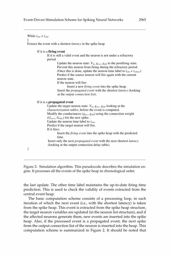
While tsim < tend { Extract the event with a shortest latency in the spike heap

If it is a firing event

If it is still a valid event and the neuron is not under a refractory period

Update the neuron state: Vm, gexc, ginh to the postfiring state. Prevent this neuron from firing during the refractory period. (Once this is done, update the neuron time label to tsim + trefrac).Predict if the source neuron will fire again with the current neuron state. If the neuron will fire:

Insert a new firing event into the spike heap. Insert the propagated event with the shortest latency (looking at the output connection list).

If it is a propagated event

Update the target neuron state: Vm, gexc, ginh looking at the characterization tables, before the event is computed. Modify the conductances (gexc, ginh) using the connection weight (Gexc,i, Ginh,i) for the new spike. Update the neuron time label to tsim. Predict if the target neuron will fire. If it fires:

Insert the firing event into the spike heap with the predicted time.

Insert only the next propagated event with the next shortest latency (looking at the output connection delay table).

}

Figure 2: Simulation algorithm. This pseudocode describes the simulation en-gine. It processes all the events of the spike heap in chronological order.

the last update. The other time label maintains the up-to-date firing timeprediction. This is used to check the validity of events extracted from thecentral event heap.

The basic computation scheme consists of a processing loop, in eachiteration of which the next event (i.e., with the shortest latency) is takenfrom the spike heap. This event is extracted from the spike heap structure,the target neuron variables are updated (in the neuron list structure), and ifthe affected neurons generate them, new events are inserted into the spikeheap. Also, if the processed event is a propagated event, the next spikefrom the output connection list of the neuron is inserted into the heap. Thiscomputation scheme is summarized in Figure 2. It should be noted that


Cm

Eexc EinhErest

gexc ginh grest Vm

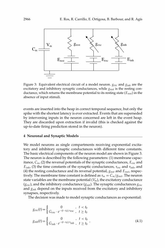
Figure 3: Equivalent electrical circuit of a model neuron. gexc and ginh are theexcitatory and inhibitory synaptic conductances, while grest is the resting con-ductance, which returns the membrane potential to its resting state (Erest) in theabsence of input stimuli.

events are inserted into the heap in correct temporal sequence, but only thespike with the shortest latency is ever extracted. Events that are supersededby intervening inputs in the neuron concerned are left in the event heap.They are discarded upon extraction if invalid (this is checked against theup-to-date firing prediction stored in the neuron).

4 Neuronal and Synaptic Models

We model neurons as single compartments receiving exponential excita-tory and inhibitory synaptic conductances with different time constants.The basic electrical components of the neuron model are shown in Figure 3.The neuron is described by the following parameters: (1) membrane capac-itance, Cm, (2) the reversal potentials of the synaptic conductances, Eexc andEinh, (3) the time constants of the synaptic conductances, τexc and τinh, and(4) the resting conductance and its reversal potential, grest and Erest, respec-tively. The membrane time constant is defined as τm = Cm/grest. The neuronstate variables are the membrane potential (Vm), the excitatory conductance(gexc), and the inhibitory conductance (ginh). The synaptic conductances gexcand ginh depend on the inputs received from the excitatory and inhibitorysynapses, respectively.

The decision was made to model synaptic conductances as exponential:

gexc(t) ={

0 , t < t0Gexc · e−(t−t0)/τexc , t ≥ t0

ginh(t) ={

0 , t < t0Ginh · e−(t−t0)/τinh , t ≥ t0

, (4.1)


Figure 4: A postsynaptic neuron receives two consecutive input spikes (top).The evolution of the synaptic conductance is the middle plot. The two excitatorypostsynaptic potentials (EPSPs) caused by the two input spikes are shown inthe bottom plot. In the solid line plots, the synaptic conductance transient isrepresented by a double-exponential expression (one exponential for the risingphase, one for the decay phase). In the dashed line plot, the synaptic conductanceis approximated by a single-exponential expression. The EPSPs produced withthe different conductance waveforms are almost identical.

where Gexc and Ginh represent the peak individual synaptic conductancesand gexc and ginh represent the total synaptic conductance of the neuron. Thisexponential representation has numerous advantages. First, it is an effectiverepresentation of realistic synaptic conductances. Thus, the improvement inaccuracy from the next most complex representation, a double-exponentialfunction, is hardly worthwhile when considering the membrane potentialwaveform (see Figure 4).

Second, the exponential conductance requires only a single state variable,because different synaptic inputs can simply be summed recursively whenupdating the total conductance:

gexc(t) = Gexc,j + e−(tcurrentspike−tpreviousspike)

gexc previous(t). (4.2)

(Gexc,j is the weight of synapse j; a similar relation holds for inhibitorysynapses). Most other representations would require additional state


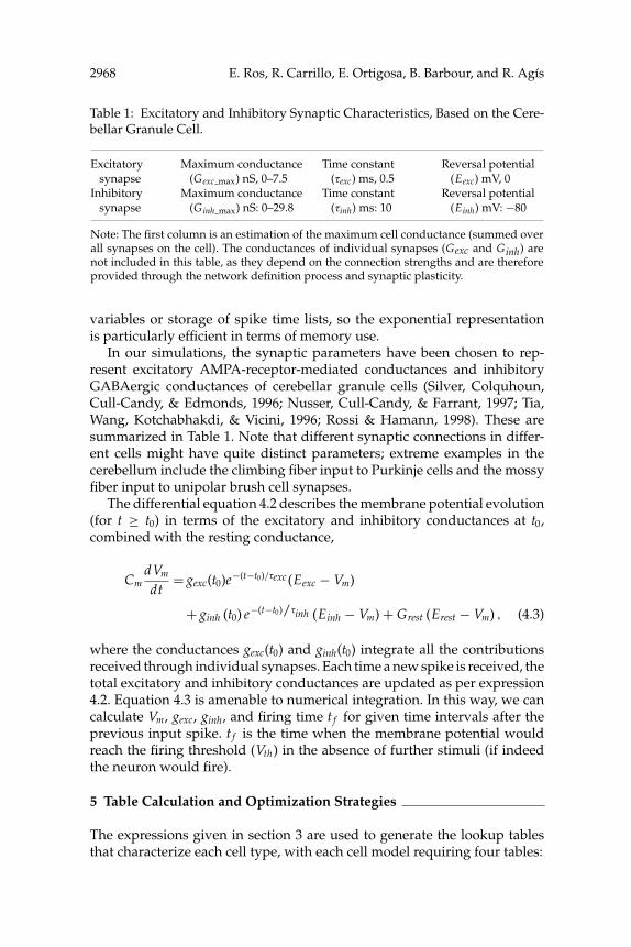
Table 1: Excitatory and Inhibitory Synaptic Characteristics, Based on the Cere-bellar Granule Cell.

Excitatorysynapse

Maximum conductance(Gexc max) nS, 0–7.5

Time constant(τexc) ms, 0.5

Reversal potential(Eexc) mV, 0

Inhibitorysynapse

Maximum conductance(Ginh max) nS: 0–29.8

Time constant(τinh) ms: 10

Reversal potential(Einh) mV: −80

Note: The first column is an estimation of the maximum cell conductance (summed overall synapses on the cell). The conductances of individual synapses (Gexc and Ginh) arenot included in this table, as they depend on the connection strengths and are thereforeprovided through the network definition process and synaptic plasticity.

variables or storage of spike time lists, so the exponential representationis particularly efficient in terms of memory use.

In our simulations, the synaptic parameters have been chosen to rep-resent excitatory AMPA-receptor-mediated conductances and inhibitoryGABAergic conductances of cerebellar granule cells (Silver, Colquhoun,Cull-Candy, & Edmonds, 1996; Nusser, Cull-Candy, & Farrant, 1997; Tia,Wang, Kotchabhakdi, & Vicini, 1996; Rossi & Hamann, 1998). These aresummarized in Table 1. Note that different synaptic connections in differ-ent cells might have quite distinct parameters; extreme examples in thecerebellum include the climbing fiber input to Purkinje cells and the mossyfiber input to unipolar brush cell synapses.

The differential equation 4.2 describes the membrane potential evolution(for t ≥ t0) in terms of the excitatory and inhibitory conductances at t0,combined with the resting conductance,

CmdVm

dt= gexc(t0)e−(t−t0)/τexc (Eexc − Vm)

+ ginh (t0) e−(t−t0)/τinh (Einh − Vm) + Grest (Erest − Vm) , (4.3)

where the conductances gexc(t0) and ginh(t0) integrate all the contributionsreceived through individual synapses. Each time a new spike is received, thetotal excitatory and inhibitory conductances are updated as per expression4.2. Equation 4.3 is amenable to numerical integration. In this way, we cancalculate Vm, gexc, ginh, and firing time t f for given time intervals after theprevious input spike. t f is the time when the membrane potential wouldreach the firing threshold (Vth) in the absence of further stimuli (if indeedthe neuron would fire).

5 Table Calculation and Optimization Strategies

The expressions given in section 3 are used to generate the lookup tablesthat characterize each cell type, with each cell model requiring four tables:


Figure 5: fg(�t), the percentage conductance remaining after a time (�t) haselapsed since the last spike was received. This is a lookup table for the normal-ized exponential function. The time constant of the excitatory synaptic conduc-tance gexc (shown here) was 0.5 ms and for ginh(t), 10 ms. Since the curve exhibitsno abrupt changes in the time interval [0, 0.0375] seconds, only 64 values wereused.

� Conductances: gexc(�t) and ginh(�t) are one-dimensional tables thatcontain the fractional conductance values as functions of the time �telapsed since the previous spike.

� Firing time: t f (Vm,t0 , gexc,t0 , ginh,t0 ) is a three-dimensional table repre-senting the firing time prediction in the absence of further stimuli.

� Membrane potential: Vm (Vm,t0 , gexc,t0 , ginh,t0 , �t) is a four-dimensional table that stores the membrane potential as a function ofthe variables at the last time that the neuron state was updated andthe elapsed time �t.

Figures 5, 6, and 7 show some examples of the contents of thesetables for a model of the cerebellar granule cell with the following para-meters: Cm = 2pF, τexc = 0.5 ms, τinh = 10 ms, grest = 0.2 nS, Eexc = 0 V,Einh = −80 mV, Erest = −70 mV, and Vth = −70 mV.

The sizes of the lookup tables do not significantly affect the processingspeed, assuming they reside in main memory (i.e., they are too large forprocessor cache but small enough not to be swapped to disk). However,their size and structure obviously influence the accuracy with which the


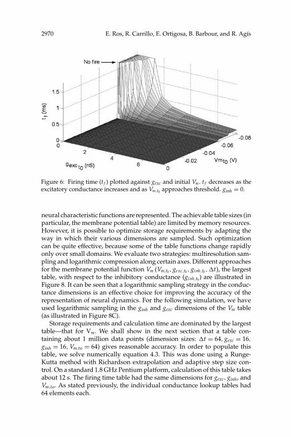
Figure 6: Firing time (t f ) plotted against gexc and initial Vm. t f decreases as theexcitatory conductance increases and as Vm,t0 approaches threshold. ginh = 0.

neural characteristic functions are represented. The achievable table sizes (inparticular, the membrane potential table) are limited by memory resources.However, it is possible to optimize storage requirements by adapting theway in which their various dimensions are sampled. Such optimizationcan be quite effective, because some of the table functions change rapidlyonly over small domains. We evaluate two strategies: multiresolution sam-pling and logarithmic compression along certain axes. Different approachesfor the membrane potential function Vm (Vm,t0 , gexc,t0 , ginh,t0 ,�t), the largesttable, with respect to the inhibitory conductance (ginh,t0 ) are illustrated inFigure 8. It can be seen that a logarithmic sampling strategy in the conduc-tance dimensions is an effective choice for improving the accuracy of therepresentation of neural dynamics. For the following simulation, we haveused logarithmic sampling in the ginh and gexc dimensions of the Vm table(as illustrated in Figure 8C).

Storage requirements and calculation time are dominated by the largesttable—that for Vm. We shall show in the next section that a table con-taining about 1 million data points (dimension sizes: �t = 64, gexc = 16,

ginh = 16, Vm,to = 64) gives reasonable accuracy. In order to populate thistable, we solve numerically equation 4.3. This was done using a Runge-Kutta method with Richardson extrapolation and adaptive step size con-trol. On a standard 1.8 GHz Pentium platform, calculation of this table takesabout 12 s. The firing time table had the same dimensions for gexc, ginh, andVm,to. As stated previously, the individual conductance lookup tables had64 elements each.


Figure 7: Membrane potential Vm(Vm,t0 , gexc,t0 , ginh,t0 , �t

)plotted as a function

of (A) Vm,t0 and �t(gexc = ginh = 0); (B) gexc,t0 and �t (ginh = 0, Vm,t0 = Erest =−70 mV). The zoom in the �t axis of plot B highlights the fact that the membranepotential change after receiving a spike is not instantaneous.

In principle, these tables could also be based on electrophysiologicalrecordings. Since one of the dimensions of the tables is the time, theexperimenter would need to set up only the initial values of gexc, ginh,and Vm and then record the membrane potential evolution following this


initial condition. With our standard table size, the experimenter would needto measure neuronal behavior for 64 × 16 × 16 (Gexc, Ginh, Vm) triplets. Ifneural behavior is recorded in sweeps of 0.5 second (at least 10 membranetime constants), only 136 minutes of recording would be required, which isfeasible (see below for ways to optimize these recordings). Characterizationtables of higher resolution would require longer recording times, but suchtables could be built up by pooling or averaging recordings from severalcells. Moreover, since the membrane potential functions are quite smooth,interpolation techniques would allow the use of smaller, easier-to-compiletables.

In order to control the synaptic conductances (gexc and ginh), it wouldbe necessary to use the dynamic clamp method (Prinz, Abbott, & Marder,2004). With this technique, it is possible to replay accurately the requiredexcitatory and inhibitory conductances. It would not be feasible to con-trol real synaptic conductances, though prior determination of their prop-erties would be used to design the dynamic clamp protocols. Dynamicclamp would most accurately represent synaptic conductances in small,electrically compact neurons (such as the cerebellar granule cells mod-eled here). Synaptic noise might distort the recordings, in which case itcould be blocked pharmacologically. Any deleterious effects of dialyaz-ing the cell via the patch pipette could be prevented by using the perfo-rated patch technique (Horn & Marty, 1988), which increases the lifetimeof the recording and ensures that the neuron maintains its physiologicalcharacteristics.

6 Simulation Accuracy

An illustrative simulation is shown in Figure 9. A single cell with the char-acteristics of a cerebellar granule cell receives excitatory and inhibitoryspikes (upper plots). We can see how the membrane conductances changeabruptly due to the presynaptic spikes. The conductance tables emulate theexcitatory AMPA-receptor-mediated and the inhibitory GABAergic synap-tic inputs (the inhibitory inputs have a longer time constant). The conduc-tance transients (excitatory and inhibitory) are also shown. The bottom plotshows a comparison between the event-driven simulation scheme, whichupdates the membrane potential at each input spike (these updates are

Figure 8: Each panel shows 16 Vm relaxations with different values of ginh,t0 .The sampled conductance interval is ginh,t0 ∈ [0,20]nS. (A) Linear approach:[0,20]nS was sampled with a constant intersample distance. (B) Multiresolutionapproach: two intervals [0,0.35]nS and [0.4,20]nS with eight traces each wereused. (C) Logarithmic approach: ginh,t0 was sampled logarithmically.


Figure 9: Single neuron simulation. Excitatory and inhibitory spikes are indi-cated on the upper plots. Excitatory and inhibitory conductance transients areplotted in the middle plots. The bottom plot is a comparison between the neuralmodel simulated with iterative numerical calculation (continuous trace) and theevent-driven scheme, in which the membrane potential is updated only whenan input spike is received (marked with an x).

marked with an x) and the results of an iterative numerical calculation(Euler method with a time step of 0.5 µs). This plot also includes the outputspikes produced when the membrane potential reaches the firing thresh-old. The output spikes are not coincident with input events, althoughthis is obscured by the timescale of the figure. It is important to notethat the output spikes produced by the event-driven scheme are coinci-dent with those of the Euler simulation (they superimpose in the bottomplot). Each time a neuron receives an input spike, both its membrane po-tential and the predicted firing time of the cell are updated. This occursonly rarely, as the spacing of the events in the event-driven simulationillustrates.

It is difficult to estimate the appropriate size of the tables for a givenaccuracy. One of the goals of this simulation scheme is to be able to simulateaccurately large populations of neurons, faithfully reproducing phenomenasuch as temporal coding and synchronization processes. Therefore, we areinterested in reproducing the exact timing of the spikes emitted. In orderto evaluate this, we need a way to quantify the difference between twospike trains. We used the van Rossum (2001) distance between two spiketrains. This is related to the distance introduced by Victor and Purpura(1996, 1997), but is easier to calculate, with expression 6.1 and has a more


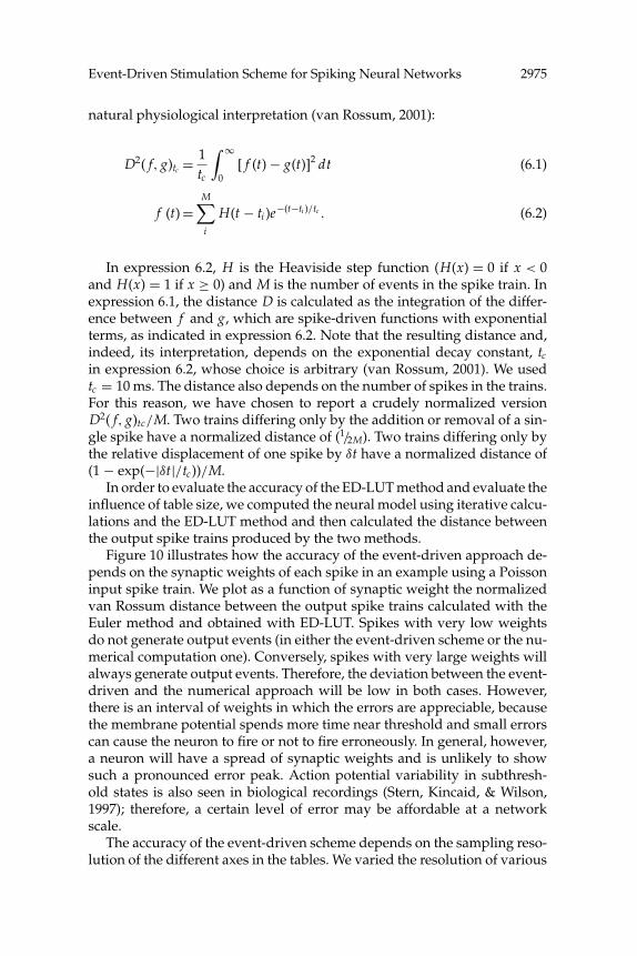
natural physiological interpretation (van Rossum, 2001):

D2( f, g)tc = 1tc

∫ ∞

0[ f (t) − g(t)]2 dt (6.1)

f (t) =M∑i

H(t − ti )e−(t−ti )/tc . (6.2)

In expression 6.2, H is the Heaviside step function (H(x) = 0 if x < 0and H(x) = 1 if x ≥ 0) and M is the number of events in the spike train. Inexpression 6.1, the distance D is calculated as the integration of the differ-ence between f and g, which are spike-driven functions with exponentialterms, as indicated in expression 6.2. Note that the resulting distance and,indeed, its interpretation, depends on the exponential decay constant, tcin expression 6.2, whose choice is arbitrary (van Rossum, 2001). We usedtc = 10 ms. The distance also depends on the number of spikes in the trains.For this reason, we have chosen to report a crudely normalized versionD2( f, g)tc/M. Two trains differing only by the addition or removal of a sin-gle spike have a normalized distance of (1/2M). Two trains differing only bythe relative displacement of one spike by δt have a normalized distance of(1 − exp(−|δt|/tc))/M.

In order to evaluate the accuracy of the ED-LUT method and evaluate theinfluence of table size, we computed the neural model using iterative calcu-lations and the ED-LUT method and then calculated the distance betweenthe output spike trains produced by the two methods.

Figure 10 illustrates how the accuracy of the event-driven approach de-pends on the synaptic weights of each spike in an example using a Poissoninput spike train. We plot as a function of synaptic weight the normalizedvan Rossum distance between the output spike trains calculated with theEuler method and obtained with ED-LUT. Spikes with very low weightsdo not generate output events (in either the event-driven scheme or the nu-merical computation one). Conversely, spikes with very large weights willalways generate output events. Therefore, the deviation between the event-driven and the numerical approach will be low in both cases. However,there is an interval of weights in which the errors are appreciable, becausethe membrane potential spends more time near threshold and small errorscan cause the neuron to fire or not to fire erroneously. In general, however,a neuron will have a spread of synaptic weights and is unlikely to showsuch a pronounced error peak. Action potential variability in subthresh-old states is also seen in biological recordings (Stern, Kincaid, & Wilson,1997); therefore, a certain level of error may be affordable at a networkscale.

The accuracy of the event-driven scheme depends on the sampling reso-lution of the different axes in the tables. We varied the resolution of various


Figure 10: The accuracy of the event-driven simulation depends on the weightsof the synapses, with maximal error (normalized van Rossum distance) occur-ring over a small interval of critical conductances. All synaptic weights wereequal.

parameters and quantified the normalized van Rossum distance of the spiketrains produced, with respect to the “correct” output train obtained froman iterative solution. The axes of the Vm and t f table were varied together,but the conductance lookup tables were not modified. Effective synapticweights were drawn at random from an interval of [0.5, 2] nS, thus cover-ing the critical interval illustrated in Figure 10. From Figure 11 we see thatthe accuracy of �t and gexc is critical, but the accuracy of the event-drivenscheme becomes more stable when table dimensions are above 1000 Ksamples. Therefore, we consider appropriate resolution values are the fol-lowing: 16 values for gexc,t0 and ginh,t0 , 64 values for �t, and 64 values forVm,t0 . These dimensions will be used henceforth.

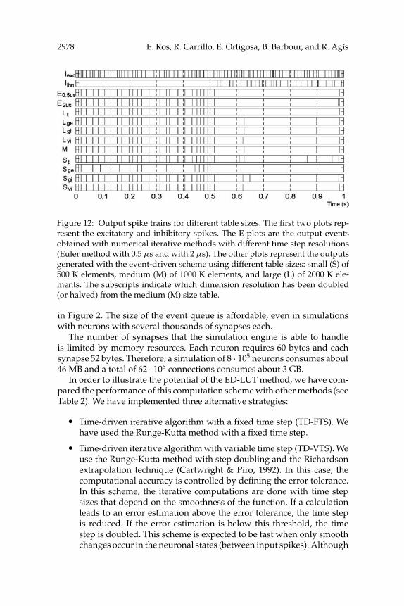
Illustrative output spike trains for different table sizes, as well as thereference train, are shown in Figure 12. The spike trains obtained withthe iterative method and the event-driven scheme are very similar for thelarge table with increased resolution in �t. A spurious spike difference isobserved in the other simulations. Doubling the resolution in dimensionsother than �t does not increase the accuracy in this particular simulation.We can also see how the spike train obtained with the small tables is signif-icantly different. This is consistent with the accuracy study results shownin Figure 11.


Figure 11: The accuracy of the event-driven approach depends on the resolutionof the different dimensions and therefore on the table sizes. To evaluate theinfluence of table size on accuracy, we ran the simulations with different tablesizes. For this purpose, we chose an initial Vm table of 1000 K samples (64 valuesfor �t, 16 values for gexc,t0 , 16 values for ginh,t0 , and 64 values for Vm,t0 ). Wethen halved the size of individual dimensions, obtaining tables of size 500 Ksamples and 250 K samples from the original table of 1000 K samples. Finally,we doubled the sampling density of individual dimensions to obtain the largesttables of 2000 K samples. For each accuracy estimation, we used an input trainof 100 excitatory and 33 inhibitory spikes generating 26 output spikes (whensimulated with iterative methods and very high temporal resolution).

7 Simulation Performance and Comparisons with Other Methods

With ED-LUT as described, the simulation time is essentially independentof the network size, depending principally on the rate of events that need tobe processed. In other words, the simulation time depends on the networkactivity, as illustrated in Figure 13.

This implementation allows, for instance, the simulation of 8 · 104 neu-rons in real time with an average firing rate of 10 Hz on a 1.8 GHz PentiumIV platform. This implies the computation at a rate of 8 · 105 spikes per sec-ond as illustrated in Figure 13. Large numbers of synaptic connections ofsingle neurons are efficiently managed by the two-stage strategy described


Figure 12: Output spike trains for different table sizes. The first two plots rep-resent the excitatory and inhibitory spikes. The E plots are the output eventsobtained with numerical iterative methods with different time step resolutions(Euler method with 0.5 µs and with 2 µs). The other plots represent the outputsgenerated with the event-driven scheme using different table sizes: small (S) of500 K elements, medium (M) of 1000 K elements, and large (L) of 2000 K ele-ments. The subscripts indicate which dimension resolution has been doubled(or halved) from the medium (M) size table.

in Figure 2. The size of the event queue is affordable, even in simulationswith neurons with several thousands of synapses each.

The number of synapses that the simulation engine is able to handleis limited by memory resources. Each neuron requires 60 bytes and eachsynapse 52 bytes. Therefore, a simulation of 8 · 105 neurons consumes about46 MB and a total of 62 · 106 connections consumes about 3 GB.

In order to illustrate the potential of the ED-LUT method, we have com-pared the performance of this computation scheme with other methods (seeTable 2). We have implemented three alternative strategies:

� Time-driven iterative algorithm with a fixed time step (TD-FTS). Wehave used the Runge-Kutta method with a fixed time step.

� Time-driven iterative algorithm with variable time step (TD-VTS). Weuse the Runge-Kutta method with step doubling and the Richardsonextrapolation technique (Cartwright & Piro, 1992). In this case, thecomputational accuracy is controlled by defining the error tolerance.In this scheme, the iterative computations are done with time stepsizes that depend on the smoothness of the function. If a calculationleads to an error estimation above the error tolerance, the time stepis reduced. If the error estimation is below this threshold, the timestep is doubled. This scheme is expected to be fast when only smoothchanges occur in the neuronal states (between input spikes). Although


Figure 13: The time taken to simulate 1 second of network activity on a PentiumIV (1.8 GHz) platform. Global activity represents the total number of spikes persecond in the network. The network size did not have a significant impact on thetime required. The time was almost linear with respect to network activity. Thehorizontal grid represents the real-time simulation limit—1 second of simulationrequiring 1 second of computation.

this method is time driven, its computation speed depends on the cellinput in the sense that the simulation passes quickly through timeintervals without input activity, and when an input spike is received,the computation approach reduces the time step to simulate accuratelythe transient behavior of the cell. A similar simulation scheme witheither global or independent variable time step integration has beenadopted in NEURON (Hines & Carnevale, 2001; Lytton & Hines, 2005).

� Pseudoanalytical approximation (PAA) method. In this case we haveapproximated the solution of the differential equations that governthe cell. In this way we can adopt an event-driven scheme similar tothat proposed in Makino (2003) and Mattia and Del Giudice (2000),in which the neuron behavior is described with analytical expres-sions. As in Makino (2003), the membrane potential is calculated withthe analytical expression, and the firing time is calculated using aniterative method based on Newton-Raphson. Since the differentialequations defining the cell behavior of our model have no analyticalsolution, we need to approximate a four-dimensional function. Evenusing advanced mathematical tools, this represents a hard task. Theaccuracy of this approach depends significantly on how good this


Table 2: Performance Evaluation of Different Methods: Accuracy versus Com-puting Time Trade-Off.

Normalized vanRossum Distance

ComputingTime (s)

Time step (s)Time driven with 56 · 10−5 0.061 0.286

fixed time step 43 · 10−5 0.033 0.363(TD-FTS) 34 · 10−5 0.017 0.462

Error toleranceTime driven with 68 · 10−5 0.061 0.209

variable time step 18 · 10−5 0.032 0.275(TD-VTS) 2 · 10−5 0.017 0.440

Pseudoanalyticalapproximation 0.131 0.142method (PAA)

Table size (106 samples)Lookup-table-based 1.05 0.061 0.0066

event-driven 6.29 0.032 0.0074scheme (ED-LUT) 39.32 0.017 0.0085

Note: We have focused on the computation of a single neuron with an input spike traincomposed of 100 seconds of excitatory and inhibitory input spikes (average input rate200 Hz) and 100 seconds of only excitatory input spikes (average input rate 10 Hz).Both spike trains had a standard deviation of 0.2 in the input rate and random weights(uniform distribution) in the interval [0,0.8] nS for the excitatory inputs and [0,1] nS forthe inhibitory inputs.

approximation is. In order to illustrate the complexity of the completecell behavior, it is worth mentioning that the expression used wascomposed of 15 exponential functions. As shown in Table 2, even thiscomplex approximation does not provide sufficient accuracy, but wehave nevertheless used it in order to estimate the computation timeof this event-driven scheme.

� Event driven based on lookup tables (ED-LUT). This is our approach,in which the transient response of the cell and the firing time of thepredicted events are computed off-line and stored in lookup tables.During the simulations, each neuronal state update is performed bytaking the appropriate value from these supporting tables.

In order to determine the accuracy of the results, we obtained the “cor-rect” output spike train using a time-driven scheme with a very short timestep. The accuracy of each method was then estimated by calculating thevan Rossum distance (van Rossum, 2001) between the obtained result and“correct” spike train.

In all methods except the pseudoanalytical approach, the accuracy versuscomputation time trade-off is managed with a single parameter (time step


in TD-FTS, error tolerance in TD-VTS, and table size in ED-LUT). We havechosen three values for these parameters that facilitate the comparisonbetween different methods (i.e., values that lead to similar accuracy values).It is worth mentioning that all methods except the time-driven with fixedtime step require a computation time that depends on the activity of thenetwork.

Table 2 illustrates several points:

� The computing time using tables (ED-LUT) of very different sizes isonly slightly affected by the memory resource management units.

� The event-driven method based on analytical expressions is more thanan order of magnitude slower than ED-LUT (and has greater error).This is caused by the complexity of the analytical expression and thecalculation of the firing time using the membrane potential expressionand applying the Newton-Raphson method.

� The ED-LUT method is about 50 times faster than the time-drivenschemes (with an input average activity of 105 Hz).

8 Discussion

We have implemented an event-driven network simulation scheme basedon precalculated neural characterization tables. The use of such tables offersflexibility in the design of cell models while enabling rapid simulations oflarge-scale networks. The main limitation of the technique arises from thesize of the tables for more complex neuronal models.

The aim of our method is to enable simulation of neural structures ofreasonable size, based on cells whose characteristics cannot be described bysimple analytical expressions. This is achieved by defining the neural dy-namics using precalculated traces of their internal variables. The proposedscheme efficiently splits the computational load into two different stages:

� Off-line neuronal model characterization. This preliminary stage re-quires a systematic numerical calculation of the cell model in differentconditions to scan its dynamics. The goal of this stage is to build upthe neural characterization tables. This can be done by means of alarge numerical calculation and the use of detailed neural simulatorssuch as NEURON (Hines & Carnevale, 1997) or GENESIS (Bower &Beeman, 1998). In principle, this could even be done by compilingelectrophysiological recordings (as described in section 6).

� Online event-driven simulation. The computation of the simulationprocess jumps from one event to the next, updating the neuron statesaccording to precalculated neuron characterization tables and effi-ciently managing newly produced events.


The proposed scheme represents a simulation tool that is intermedi-ate between the very detailed simulators, such as NEURON (Hines &Carnevale, 1997) or GENESIS (Bower & Beeman, 1998), and the event-drivensimulation schemes based on simple analytically described cell dynamics(Delorme et al., 1999; Delorme & Thorpe, 2003). The proposed scheme isable to capture cell dynamics from detailed simulators and accelerate thesimulation of large-scale neural structures. The approach as implementedhere allows the simulation of 8 · 104 neurons with up to 6 · 107 connectionsin real time with an average firing rate of 10 Hz on a 1.8 GHz Pentium IVplatform.

It is difficult to make a precise performance comparison between ourmethod and previous event-driven methods, since they are based on dif-ferent neuron models. Nevertheless, we have evaluated different computa-tional strategies to illustrate the potential of our approach (see section 7).Mattia and Del Giudice (2000) used a cell model whose dynamics are de-fined by simple analytical expressions, and Reutimann et al. (2003) extendedthis approach by including stochastic dynamic. They avoided numericalmethods by using precalculated lookup tables. In this case, provided that thereordering event structure is kept of reasonable size (in those approaches,large, divergent connection trees may overload the spike reordering struc-ture), the computation speed of these schemes is likely to be comparable toour approach, since the evaluation of a simple analytical expression and alookup table consultation consume approximately the same time.

The method has been applied to simulations containing one-compartment cell models with exponential synaptic conductances (with dif-ferent time constants) approximating excitatory AMPA receptor-mediatedand GABAergic inhibitory synaptic inputs. The inclusion of new mecha-nisms, such as voltage-dependent channels, is possible. However it wouldrequire the inclusion of new neural variables and thus new table dimen-sions. Although very complex models may eventually require lookup tablesthat exceed current memory capacities, we have shown how even a modestnumber of table dimensions can suffice to represent quite realistic neu-ronal models. We have also evaluated several strategies for compressingthe tables in order to accommodate more complex models. Furthermore, inappendix C, the proposed table-based methodology is used to simulate theHodgkin and Huxley model (1952).

The event-driven scheme could be used for multicompartment neuronmodels, although each compartment imposes a requirement for additional(one to three) dimensions in the largest lookup table. There are two waysin which multicompartment neurons may be partially or approximatelyrepresented in this scheme. After preliminary studies, using suitable sam-pling schemes in order to achieve reasonable accuracy with a restrictedtable size, we can manage lookup tables of reasonable accuracy with morethan seven dimensions. Therefore, we can add two extra dimensions toenable two-compartment simulations. Quite rich cellular behavior could


be supplied by this extension. More concretely, we plan the addition of asecond electrical compartment containing an inhibitory conductance. Thisnew compartment will represent the soma of a neuron, while the originalcompartment (containing both excitatory and inhibitory conductances) willrepresent the dendrites. The somatic voltage and inhibitory conductancerequire two additional dimensions in the lookup table. With this model, itwould be possible to separate somatic and dendritic processing, as occursin hippocampal and cortical pyramidal cells, and implement the differen-tial functions of somatic and dendritic inhibition (Pouille & Scanziani, 2001,2004) (note that most neurons do not receive excitation to the soma).

If individual dendrites can be active and have independent computa-tional functions (this is currently an open question), it may be possible toapproximate the dendrites and soma of a neuron as a kind of two-layernetwork (Poirazi, Brannon, & Mel, 2003), in which dendrites are actuallyrepresented in a manner similar to individual cells, with spikes that arerouted to the soma (another cell) in the standard manner.

We have embedded spike-driven synaptic plasticity mechanisms (seeappendix B) in the event-driven simulation scheme. For this purpose, wehave implemented learning rules approximated by exponential terms thatcan be computed recursively using an intermediate variable. Short-termdynamics (Mattia & Del Guidice, 2000) are also easy to include in the simu-lations. They are considered important in the support of internal stimulusrepresentation (Amit, 1995; Amit & Brunel, 1997a, 1997b) and learning.

In summary, we have implemented, optimized, and evaluated an event-driven network simulation scheme based on prior characterization of allneuronal dynamics, allowing simulation of large networks to proceed ex-tremely rapidly by replacing all function evaluations with table lookups.Although very complex neuronal models would require unreasonably largelookup tables, we have shown that careful optimization nevertheless per-mits quite rich cellular models to be used. We believe ED-LUT will providea useful addition to available simulation tools.

This software package is currently being evaluated in the context of real-time simulations in four labs in different institutions. We plan to extend itsuse to other labs in the near future. The software is available on request fromthe authors. Using this method, neural systems of reasonable complexityare already being simulated in real time, in experiments related to robotcontrol by bio-inspired processing schemes (Boucheny, Carrillo, Ros, &Coenen, 2005).

Appendix A: Event Data Structure

Complex data structures, such as balanced trees, can be used for this pur-pose, offering good performance for both sorted and random-order inputstreams. To prevent performance degradation, they optimize their structureafter each insertion or deletion. However, this rebalancing process adds


more complexity and additional computational overhead (Karlton, Fuller,Scroggs, & Kaehler, 1976). Insertion and deletion of elements in these struc-tures have a computational cost of O(log(N)), where N is the number ofevents in the structure.

Another candidate data structure is the “skip list” (Pugh, 1990), but inthis instance, the cost of the worst case may not be O(log(N)) because theinsertion of an input stream can produce an unbalanced structure. Con-sequently, the search time for a new insertion may be longer than in thebalanced trees. This structure offers optimal performance in searching spe-cific elements. However, this is not needed in our computation scheme aswe need to extract only the first element (i.e., the next spike).

Finally, the heap data structure (priority queue) (Aho, Hopcroft, &Ullman, 1974; Chowdhury & Kaykobad, 2001; Cormen, Lierson, & Rivest,1990) offers a stable computational cost of O(log(N)) in inserting and delet-ing elements. This is the best option as it does not require more memoryresources than the stored data. This is because it can be implemented as anarray, while the “balanced trees” and “skip lists” need further pointers oradditional memory resources.

For all of these methods, the basic operation of inserting an event costsroughly O(log(N)), where N is the number of events in the event datastructure. Clearly, the smaller the data structure, the less time such insertionswill take. We explain in section 3 the two-stage event handling process wehave implemented in order to minimze event heap size while allowingarbitrary divergences and latencies. Compared to a method using a single-event data structure, we would expect the event insertions to be O(log(c))quicker, where c is the average divergence (connectivity). In Figure 14, wecompare the use of one- and two-stage event handling within our simulationscheme. Although event heap operations represent only part of the totalcomputation time, there is a clear benefit to using the two-stage process.For divergences of up to 10,000, typical for recurrent cortical networks, abetter than twofold improvement of total computation time is observed.

Appendix B: Spike-Timing-Dependent Synaptic Plasticity

We have implemented Hebbian-like (Hebb, 1949) spike-driven learningmechanisms (spike-timing-dependent plasticity, STDP). The implementa-tion of such leaning rules is suitable because the simulation scheme is basedon the time labels of the different events. Spike-time-dependent learningrules require comparison of the times of presynaptic spikes (propagatedevents) with postsynaptic spikes (firing event). In principle, this requiresthe trace of the processed presynaptic spikes during a time interval to bekept in order for them to be accessible if postsynaptic spikes occur. Differentdefinite expressions can be used for the learning rule (Gerstner & Kistler,2002). The weight change function has been approximated with exponentialexpressions (see equation B.1) to accommodate the experimental results of


Figure 14: Total computation time for processing an event (top) and size of theevent heap (bottom) for one-stage (dashed plot) and two-stage (continuous plot)as functions of synaptic divergence.

Bi and Poo (1998). The computation of this learning rule, by means of ex-ponential terms, facilitates its implementation in a recursive way, avoidingthe need to keep track of previous spikes:

f (s) ={

apree−bpres i f s < 0apostebposts i f s > 0 , (B.1)

where s = tpost − tpre represents the temporal delay between the postsy-naptic spike and the presynaptic one. The aim function (Bi & Poo, 1998)can be calculated with expression B.1 using the following parameters(apre = 0.935, bpre = −0.075, apost = −0.326, bpost = −0.036). They have beenapproximated using the Trust-region method (Conn, Gould, & Toint, 2000).

The learning rules are applied each time a cell both receives and firesa spike. Each time a spike from cell i reaches a neuron j , the connectionweight (wij) is changed according to expression B.2, taking into account thetime since the last action potential (AP) in the postsynaptic neuron. Thistime is represented by s in expression B.1:

wij ← wij + �wijwhere�wij = wij f (s).

(B.2)


Other postsynaptic spikes are not taken into account for the sake of sim-plicity, but they can be included if necessary.

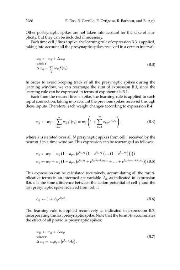
Each time cell j fires a spike, the learning rule of expression B.3 is applied,taking into account all the presynaptic spikes received in a certain interval:

wij ← wij + �wijwhere�wij = ∑

kwij f (sk).

(B.3)

In order to avoid keeping track of all the presynaptic spikes during thelearning window, we can rearrange the sum of expression B.3, since thelearning rule can be expressed in terms of exponentials B.1.

Each time the neuron fires a spike, the learning rule is applied in eachinput connection, taking into account the previous spikes received throughthese inputs. Therefore, each weight changes according to expression B.4:

wij ← wij +N∑

k=1

wij f (sk) = wij

(1 +

N∑k=1

apreebpresk

), (B.4)

where k is iterated over all N presynaptic spikes from cell i received by theneuron j in a time window. This expression can be rearranged as follows:

wij ← wij + wij(1 + apre

(ebpres1

(1 + ebpres2

(. . .

(1 + ebpresN

)))))wij ← wij + wij

(1 + apre

(ebpres1 + ebpres1+bpres2 + . . . + ebpres1+...+bpresN

)).(B.5)

This expression can be calculated recursively, accumulating all the multi-plicative terms in an intermediate variable Aij, as indicated in expressionB.6. s is the time difference between the action potential of cell j and thelast presynaptic spike received from cell i :

Aij ← 1 + Aijebpres . (B.6)

The learning rule is applied recursively as indicated in expression B.7,incorporating the last presynaptic spike. Note that the term Aij accumulatesthe effect of all previous presynaptic spikes:

wij ← wij + �wijwhere�wij = wijapre

(ebpres Aij

).

(B.7)


Table 3: Hodgkin and Huxley Model (1952).

dVmdt = (

I − gK · n4 · (Vm − VK ) − gNs · m3 · h · (Vm − VNa) − gl (Vm − Vl ))/

Cm

dndt = φ · (αn · (1 − n) − βn · n) ; dm

dt = φ · (αm · (1 − m) − βm · m) ;dhdt = φ · (αh · (1 − h) − βh · h)

αn = 0.01·Vm+0.1exp(0.1·Vm+1)−1 ; αm = 0.1·Vm+2.5

exp(0.1·Vm+2.5)−1 ; αh = 0.07 · exp (0.05 · Vm)

βn = 0.125 · exp (Vm/80) ; βm = 4 exp (Vm/18) ; βh = 1exp(0.1·Vm+3)+1

φ = 3(T−6.3)/10

I = −gexc · (Vm − Eexc) − ginh · (Vm − Einh

)dgexc

dt = − gexcτexc

; dginhdt = − ginh

τinh

Note: The first expression describes the membrane potential evolution. The differ-ential equations of n, m, and h govern the ionic currents. The last two expressions ofthe table describe the input-driven currents and synaptic conductances. The param-eters are the following: Cm = 1µ F/cm2, gK = 1 mS/cm2, gNa = 120 mS/cm2, gl =0.3 mS/cm2, VNa = −115 mV, VK = 12 mV, Vl = −10.613 mV, and T = 6.3oC . Theparameters of the synaptic conductances are the following: Eexc = −65 mV, Einh =15 mV, τexc = 0.5 ms, and τinh = 10 ms.

Appendix C: Hodgkin and Huxley Model

In order to further validate the simulation scheme, we have also compiledinto tables the Hodgkin and Huxley model (1952) and evaluated the accu-racy obtained with the proposed table-based methodology. Table 3 showsthe differential expressions that define the neural model. We have also in-cluded expressions for synaptic conductances.

Interfacing the explicit representation of the action potential to the event-handling architecture, which is based on idealized instantaneous actionpotentials, raises a couple of technical issues. The first is the choice of theprecise time point during the action potential that should correspond tothe idealized (propagated) event. This choice is arbitrary; we chose thepeak of the action potential. The second issue arises from the interactionof this precise time point with discretization errors during updates closeto the peak of the action potential. As illustrated in Figure 15, a simple-minded implementation can cause the duplication (or by an analogousmechanism, omission) of action potentials, a significant error. This canhappen when an update is triggered by an input arriving just after thepeak of the action potential (and thus after the propagated event). Dis-cretization errors can cause the prediction of the peak in the immediatefuture, equivalent to a very slight shift to the right of the action poten-tial waveform. Since we have identified the propagated event with thepeak, a duplicate action potential would be emitted. The frequency of such


Figure 15: Discretization errors could allow an update shortly following anaction potential peak to predict the peak of the action potential in the immediatefuture, leading to the emission of an erroneous duplicate spike. (The errors havebeen magnified for illustrative purposes.)

errors depends on the discretization errors and thus the accuracy (size) ofthe lookup tables and on the frequency of inputs near the action potentialpeaks. These errors are likely to be quite rare, but as we now explain, theycan be prevented.

We now describe one possible solution (which we have implemented) tothis problem (see Figure 16). We define a “firing threshold” (θ f ; in practice,−10 mV). This is quite distinct from the physiological threshold, which ismuch more negative. If the membrane potential exceeds θ f , we considerthat an action potential will be propagated under all conditions. We exploitthis assumption by always predicting a propagated event if the membranepotential is greater than θ f after the update, even if the “present” is afterthe action potential peak (in this case, emission is immediate). This proce-dure ensures that no action potentials are omitted, leaving the problem ofduplicates.

We also define a postemission time window. This extends from the timeof emission (usually the action potential peak) to the time the membrane


Figure 16: Prevention of erroneous spike omission and duplication. Once theneuron exceeds θ f , a propagated event is ensured. In this range, updates thatcause the action potential peak to be skipped cause immediate emission. Thisprevents action potential omission. Once the action potential is emitted (usuallyat t f ), the time t f end is stored, and no predicted action potential emissions beforethis time are accepted. This ensures that no spikes are propagated more thanonce.

potential crosses another threshold voltage, θ f end . This time, t f end , is storedin the source neuron when the action potential is emitted. Whenever newinputs are processed, any predicted output event times are compared witht f end and only those predicted after t f end are accepted. This procedureeliminates the problem of duplicate action potentials.

In order to preserve the generality of this implementation, we chose to de-fine these windows around the action potential peak by voltage level cross-ings. In this way, the implementation will adapt automatically to changesof action potential waveform (possibly resulting from parameter changes).This choice entailed the construction of an additional large lookup table.Simpler implementations based on fixed time windows could avoid thisrequirement. However, the cost of the extra table was easily borne.


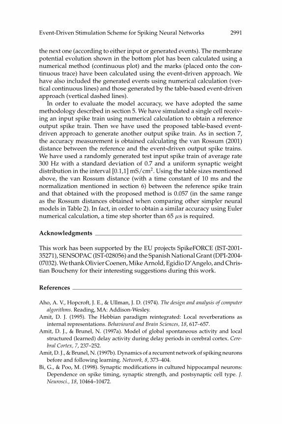
Figure 17: Single neuron event-driven simulation of the Hodgkin and Huxleymodel. Note that in order to facilitate the comparison of the plots with the onesof the integrate-and-fire model (see Figure 9) the variable (V) has been calculatedusing the following expression V = (−Vm − Vrest)/1000 with Vrest = 65 mV.

We have compiled the model into the following tables:� One table of seven dimensions for the membrane potential, Vm =

f (�t, gexc 0, ginh 0, n0, m0, h0, V0).� Three tables of seven dimensions for the variables driv-

ing ionic currents, n = f (�t, gexc 0, ginh 0, n0, m0, h0, V0), m =f (�t, gexc 0, ginh 0, n0, m0, h0, V0), h = f (�t, gexc 0, ginh 0, n0, m0, h0, V0).

� Two tables of two dimensions for the conductances, gexc =f (�t, gexc 0), ginh = f (�t, ginh 0).

� Two tables of six dimensions for the firing prediction, t f =f (gexc, ginh, n0, m0, h0, V0) and t f end = f (gexc, ginh, n0, m0, h0, V0). Withθ f = −0.01 V and θ f end = −0.04 V.

An accurate simulation of this model (as shown in Figure 17) requiresapproximately 6.15 Msamples (24.6 MB using 4-byte floating point datarepresentation) for each seven-dimension table. We use a different numberof samples for each dimension: �t(25), gexc 0(6), ginh 0(6), n0(8), m0(8), h0(8),and V0(14). The table calculation and compilation stage of this model re-quires approximately 4 minutes on a Pentium IV 1.8 Ghz.

Figure 17 shows an illustrative simulation of the Hodgkin and Huxleymodel using the table-based event-driven scheme. Note that the simulationengine is able to accurately jump from one marked instant (bottom plot) to


the next one (according to either input or generated events). The membranepotential evolution shown in the bottom plot has been calculated using anumerical method (continuous plot) and the marks (placed onto the con-tinuous trace) have been calculated using the event-driven approach. Wehave also included the generated events using numerical calculation (ver-tical continuous lines) and those generated by the table-based event-drivenapproach (vertical dashed lines).

In order to evaluate the model accuracy, we have adopted the samemethodology described in section 5. We have simulated a single cell receiv-ing an input spike train using numerical calculation to obtain a referenceoutput spike train. Then we have used the proposed table-based event-driven approach to generate another output spike train. As in section 7,the accuracy measurement is obtained calculating the van Rossum (2001)distance between the reference and the event-driven output spike trains.We have used a randomly generated test input spike train of average rate300 Hz with a standard deviation of 0.7 and a uniform synaptic weightdistribution in the interval [0.1,1] mS/cm2. Using the table sizes mentionedabove, the van Rossum distance (with a time constant of 10 ms and thenormalization mentioned in section 6) between the reference spike trainand that obtained with the proposed method is 0.057 (in the same rangeas the Rossum distances obtained when comparing other simpler neuralmodels in Table 2). In fact, in order to obtain a similar accuracy using Eulernumerical calculation, a time step shorter than 65 µs is required.

Acknowledgments

This work has been supported by the EU projects SpikeFORCE (IST-2001-35271), SENSOPAC (IST-028056) and the Spanish National Grant (DPI-2004-07032). We thank Olivier Coenen, Mike Arnold, Egidio D’Angelo, and Chris-tian Boucheny for their interesting suggestions during this work.

References

Aho, A. V., Hopcroft, J. E., & Ullman, J. D. (1974). The design and analysis of computeralgorithms. Reading, MA: Addison-Wesley.

Amit, D. J. (1995). The Hebbian paradigm reintegrated: Local reverberations asinternal representations. Behavioural and Brain Sciences, 18, 617–657.

Amit, D. J., & Brunel, N. (1997a). Model of global spontaneous activity and localstructured (learned) delay activity during delay periods in cerebral cortex. Cere-bral Cortex, 7, 237–252.

Amit, D. J., & Brunel, N. (1997b). Dynamics of a recurrent network of spiking neuronsbefore and following learning. Network, 8, 373–404.

Bi, G., & Poo, M. (1998). Synaptic modifications in cultured hippocampal neurons:Dependence on spike timing, synaptic strength, and postsynaptic cell type. J.Neurosci., 18, 10464–10472.


Boucheny, C., Carrillo, R., Ros, E., & Coenen, O. J. M. D. (2005). Real-time spikingneural network: An adaptive cerebellar model. Lecture Notes in Computer Science,3512, 136–144.

Bower, J. M., & Beeman, B. (1998). The book of GENESIS. New York: Springer-Verlag.Braitenberg, V., & Atwood, R. P. (1958). Morphological observations on the cerebellar

cortex. J. Comp. Neurol., 109, 1–33.Brunel, N., & Hakim, V. (1999). Fast global oscillations in networks of integrate-and-

fire neurons with low firing rates. Neural Computation, 11, 1621–1671.Cartwright, J. H. E., & Piro, O. (1992). The dynamics of Runge-Kutta methods. Int. J.

Bifurcation and Chaos, 2, 427–449.Chowdhury R. A., & Kaykobad, M. (2001). Sorting using heap structure. International

Journal of Computer Mathematics, 77, 347–354.Conn, A. R., Gould, N. I. M., & Toint, P. L. (2000). Trust-region methods. Philadelphia:

SIAM.Cormen, T. H., Lierson, C. E., & Rivest, R. L. (1990). Introduction to algorithms. Cam-

bridge, MA: MIT Press.Delorme, A., Gautrais, J., van Rullen, R., & Thorpe, S. (1999). SpikeNET: A simulator

for modelling large networks of integrate and fire neurons. Neurocomputing, 26–27, 989–996.

Delorme, A., & Thorpe, S. (2003). SpikeNET: An event-driven simulation packagefor modelling large networks of spiking neurons. Network: Computation in NeuralSystems, 14, 613–627.

Eckhorn, R., Bauer, R., Jordan, W., Brosh, M., Kruse, W., Munk, M., & Reitbock, H. J.(1988). Coherent oscillations: A mechanism of feature linking in the visual cortex?Biol. Cyber., 60, 121–130.

Eckhorn, R., Reitbock, H. J., Arndt, M., & Dicke, D. (1990). Feature linking viasynchronization among distributed assemblies: Simulations of results from catvisual cortex. Neural Computation, 2, 293–307.

Gerstner, W., & Kistler, W. (2002). Spiking neuron models: Single neurons, populations,plasticity. Cambridge: Cambridge University Press.

Hebb, D. O. (1949). The organization of behavior. New York: Wiley.Hines, M. L., & Carnevale, N. T. (1997). The NEURON simulation environment.

Neural Computation, 9, 1179–1209.Hodgkin, A. L., & Huxley, A. F. (1952). A quantitative description of membrane cur-

rent and its application to conduction and excitation in nerve. Journal of Physiology,117, 500–544.

Horn, R., & Marty, A. (1988). Muscarinic activation of ionic currents measured by anew whole-cell recording method. Journal of General Physiology, 92, 145–159.

Karlton, P. L., Fuller, S. H., Scroggs, R. E., & Kaehler, E. B. (1976). Performance ofheight-balanced trees. Communications of ACM, 19(1), 23–28.

Lytton, W. W., & Hines, M. L. (2005). Independent variable time-step integration ofindividual neurons for network simulations. Neural Computation, 17, 903–921.

Makino, T. (2003). A discrete-event neural network simulator for general neuronmodels. Neural Computing and Applications, 11, 210–223.

Mattia, M., & Del Giudice, P. (2000). Efficient event-driven simulation of large net-works of spiking neurons and dynamical synapses. Neural Computation, 12(10),2305–2329.


Mitchell, S. J., & Silver, R. A. (2003). Shunting inhibition modulates neuronal gainduring synaptic excitation. Neuron, 38, 433–445.

Nusser, Z., Cull-Candy, S., & Farrant, M. (1997). Differences in synaptic GABA(A)receptor number underlie variation in GABA mini amplitude. Neuron, 19(3), 697–709.

Poirazi, P., Brannon, T., & Mel, B. W. (2003). Pyramidal neuron as two-layer neuralnetwork. Neuron, 37(6), 989–999.

Pouille, F., & Scanziani, M. (2001). Enforcement of temporal fidelity in pyramidalcells by somatic feed-forward inhibition. Science, 293(5532), 1159–1163.

Pouille, F., & Scanziani, M. (2004). Routing of spike series by dynamic circuits in thehippocampus. Nature, 429(6993), 717–723.

Prinz, A. A., Abbott, L. F., & Marder, E. (2004). The dynamic clamp comes of age.Trends Neurosci., 27, 218–224.

Pugh, W. (1990). Skip lists: A probabilistic alternative to balanced trees. Communica-tions of the ACM, 33(6), 668–676.

Reutimann, J., Giugliano, M., & Fusi, S. (2003). Event-driven simulation of spikingneurons with stochastic dynamics. Neural Computation, 15, 811–830.

Rossi, D. J., & Hamann, M. (1998). Spillover-mediated transmission at inhibitorysynapses promoted by high affinity alpha6 subunit GABA(A) receptors andglomerular geometry. Neuron, 20(4), 783–795.

Silver, R. A., Colquhoun, D., Cull-Candy, S. G., & Edmonds, B. (1996). Deactivationand desensitization of non-NMDA receptors in patches and the time course ofEPSCs in rat cerebellar granule cells. J. Physiol., 493(1), 167–173.

Stern, E. A., Kincaid, A. E., & Wilson, C. J. (1997). Spontaneous subthreshold mem-brane potential fluctuations and action potential variability of rat corticostriataland striatal neurons in vivo. J. Neurophysiol., 77, 1697–1715.

Tia, S., Wang, J. F., Kotchabhakdi, N., & Vicini, S. (1996). Developmental changesof inhibitory synaptic currents in cerebellar granule neurons: Role of GABA(A)receptor alpha 6 subunit. J. Neurosci., 16(11), 3630–3640.

van Rossum, M. C. W. (2001). A novel spike distance. Neural Computation, 13, 751–763.Victor, J. D., & Purpura, K. P. (1996). Nature and precision of temporal coding in

visual cortex: A metric-space analysis. J. Neurophysiol., 76, 1310–1326.Victor, J. D., & Purpura, K. P. (1997). Metric-space analysis of spike trains: Theory,

algorithms and application. Network: Computation in Neural Systems, 8, 127–164.Watts, L. (1994). Event-driven simulation of networks of spiking neurons. In J. D.

Cowan, G. Tesauro, & J. Alspector (Eds.), Advances in neural information processingsystems, 6 (pp. 967–934). San Mateo, CA: Morgan Kaufmann.

Received November 30, 2004; accepted April 28, 2006.

Event-Driven Simulation Scheme for Spiking Neural...

Documents

Transcript of Event-Driven Simulation Scheme for Spiking Neural...