Evan Girvetzgirvetz@u.washington.edu

206-543-5772

209 Winkenwerder

Intro to R Programming: Lecture 2

© R Foundation, from http://www.r-project.org

Overview

• Reading data into R (e.g. from Excel)

• Working with and manipulating data frames

• Writing data to text files to use in Excel

Finding the Right Command

There are many ways to find the correct command to read data files

1.Use help.search

> help.search(“read data table”)

2. Look in reference material (e.g. Ref Card)

3. Use Google

Google “Read data table R”

Finding the Right Command

read.table()

read.csv()

scan()

Look at these using R help?read.table

help(read.table)

Commands for Reading Data Tables

Commands are the same except for defaults:

read.table: general table reading command (tab delimited default)

read.csv: comma separated values

scan: good for reading odd formatting

I use read.csv the most

Reading Data into R

• It is best to prepare your data in Excel (or other spreadsheet program.

– That is what they are made for

Reading Data into R

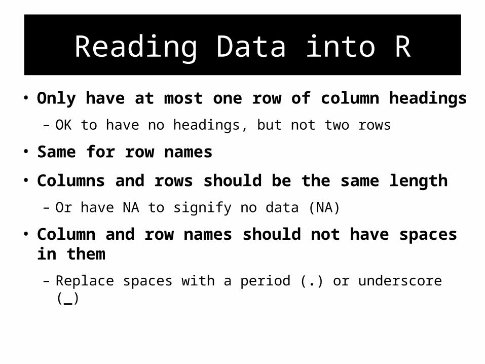
• Only have at most one row of column headings

– OK to have no headings, but not two rows

• Same for row names

• Columns and rows should be the same length

– Or have NA to signify no data (NA)

• Column and row names should not have spaces in them

– Replace spaces with a period (.) or underscore (_)

Hands-On Exercise

• Open the file “chinook_adult_return_data.xls”

Reading Data into R

• Try to “clean-up” data as best as possible in Spreadsheet program

What are some of the problems with the excel file?

Reading Data into R

• Only have at most one row of column headings

– OK to have no headings, but not two rows

• Same for row names

• Columns and rows should be the same length

– Or have NA to signify no data (NA)

• Column and row names should not have spaces in them

– Replace spaces with a period (.) or underscore (_)

Reading Data into R

• Save data from Excel in text format

– e.g. .csv or .txt (I like .csv)

• Make sure you know what are the delimiters that separate the data

– This a comma for .csv, likely a tab or white space for .txt

Hands-On Exercise

• Clean up the Adult Chinook Return Data in Excel

• Export to two text files (.csv and .txt)

• Open the exported files in a text editor

– e.g. Notepad, Wordpad, Tinn-R

read.table

• Look at the help for read.table and read.csv

> ?read.table

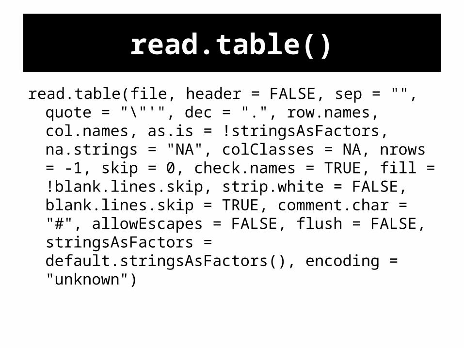
read.table()

read.table(file, header = FALSE, sep = "", quote = "\"'", dec = ".", row.names, col.names, as.is = !stringsAsFactors, na.strings = "NA", colClasses = NA, nrows = -1, skip = 0, check.names = TRUE, fill = !blank.lines.skip, strip.white = FALSE, blank.lines.skip = TRUE, comment.char = "#", allowEscapes = FALSE, flush = FALSE, stringsAsFactors = default.stringsAsFactors(), encoding = "unknown")

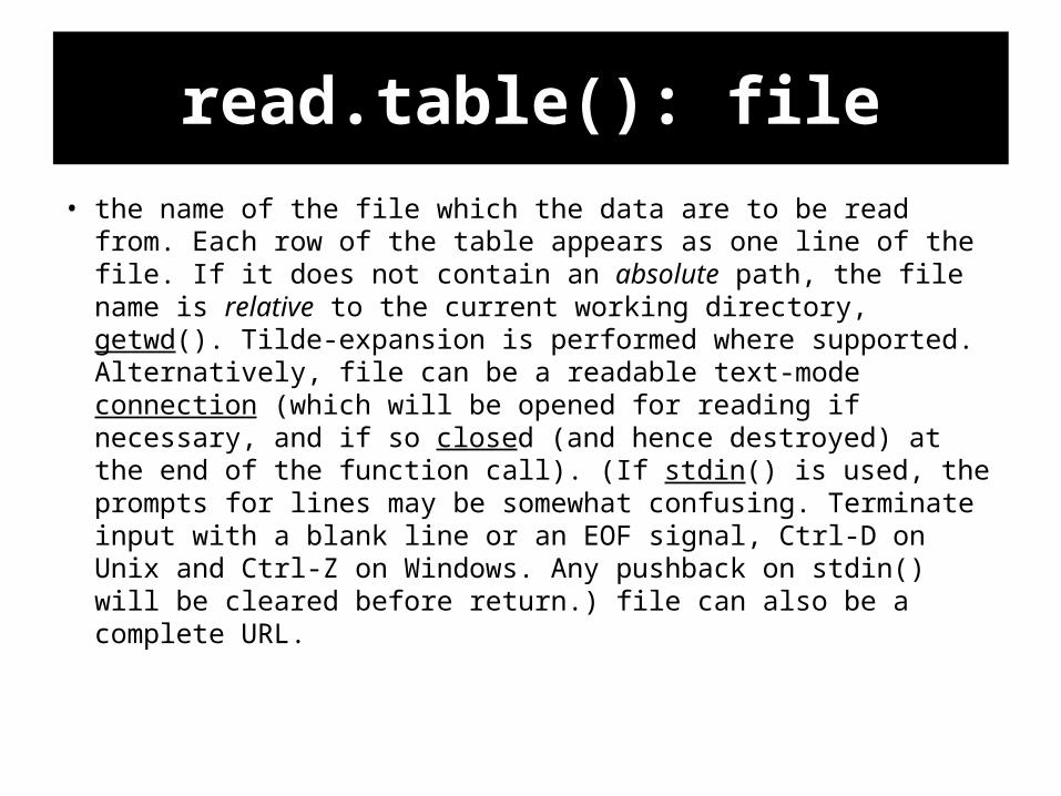
read.table(): file

• the name of the file which the data are to be read from. Each row of the table appears as one line of the file. If it does not contain an absolute path, the file name is relative to the current working directory, getwd(). Tilde-expansion is performed where supported. Alternatively, file can be a readable text-mode connection (which will be opened for reading if necessary, and if so closed (and hence destroyed) at the end of the function call). (If stdin() is used, the prompts for lines may be somewhat confusing. Terminate input with a blank line or an EOF signal, Ctrl-D on Unix and Ctrl-Z on Windows. Any pushback on stdin() will be cleared before return.) file can also be a complete URL.

read.table(): header

• a logical value indicating whether the file contains the names of the variables as its first line. If missing, the value is determined from the file format: header is set to TRUE if and only if the first row contains one fewer field than the number of columns.

read.table(): sep

• the field separator character. Values on each line of the file are separated by this character. If sep = "" (the default for read.table) the separator is ‘white space’, that is one or more spaces, tabs, newlines or carriage returns.

read.table(): quote

• the set of quoting characters. To disable quoting altogether, use quote = "". See scan for the behaviour on quotes embedded in quotes. Quoting is only considered for columns read as character, which is all of them unless colClasses is specified.

read.table(): rownames

• a vector of row names. This can be a vector giving the actual row names, or a single number giving the column of the table which contains the row names, or character string giving the name of the table column containing the row names. If there is a header and the first row contains one fewer field than the number of columns, the first column in the input is used for the row names. Otherwise if row.names is missing, the rows are numbered. Using row.names = NULL forces row numbering. Missing or NULL row.names generate row names that are considered to be ‘automatic’ (and not preserved by as.matrix).

read.table(): colnames

• a vector of optional names for the variables. The default is to use "V" followed by the column number

Commands for Reading Data Tables

Commands are the same except for defaults:

read.table: general table reading command (tab delimited default)

read.csv: comma separated values

read.delim: tab delimited values

Reading Tables: Defaults

SeparatorDecimal Symbol

Header Default

read.table

read.csv

read.delim

Hands-On Exercise

• Read both exported data files (the .txt and the .csv) into R objects called:

adultReturn (for the .csv)

and

adultReturnTxt (for the .txt)

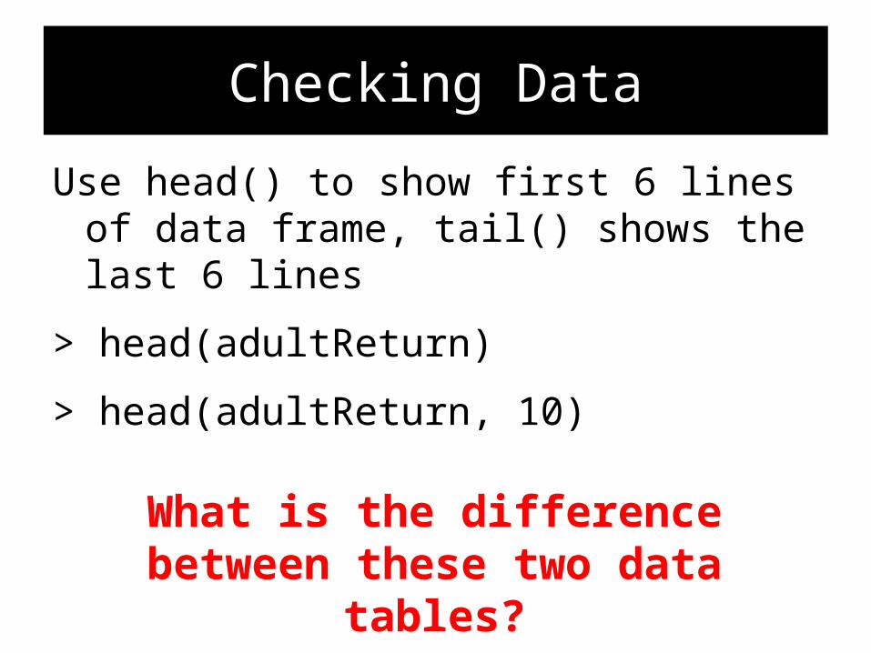
Checking Data

Use head() to show first 6 lines of data frame, tail() shows the last 6 lines

> head(adultReturn)

> head(adultReturn, 10)

> head(adultReturnTxt)

> tail(adultReturn, 10)What is the difference between these two data tables?

read.table

• Read.table needs the argument header=T to read in the column headings

> adultReturnTxt <-

+ read.table(“chinook_adult_return_data.txt”,

+ header = T)

Read data using scan

• Look at help for scan

> ?scan

Read data using scan

> adultReturnScan <-scan

+ ("chinook_adult_return_data.txt")

> adultReturnScan

> ?scan

This does not look very good…

Read data using scan

> adultReturnScan <-scan

+ ("chinook_adult_return_data.txt“,

+ what = list(“”,””,””,””,””,””))

> adultReturnScan

> ?scan

This looks better, but the column headers are with the data

Read data using scan

> adultReturnScan <-scan

+ ("chinook_adult_return_data.txt“,

+ what = list(“”,””,””,””,””,””),

+ skip = 1)

> adultReturnScan

We can work with this.

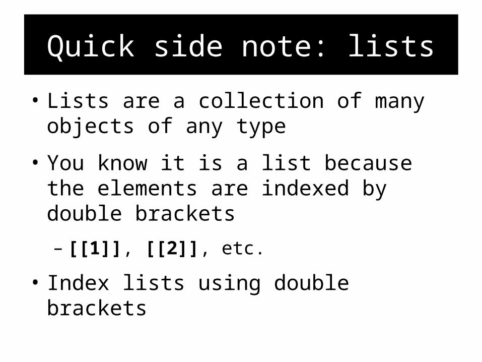
Quick side note: lists

• Lists are a collection of many objects of any type

• You know it is a list because the elements are indexed by double brackets

– [[1]], [[2]], etc.

• Index lists using double brackets

Indexing Lists

Get the fifth element of the list:

> adultReturnScan[[5]]

First 10 entries of the fifth element

> firstElement <- adultReturnScan[[5]][1:10]

> firstElement[1:10]

Do this shorter:

> adultReturnScan[[5]][1:10]

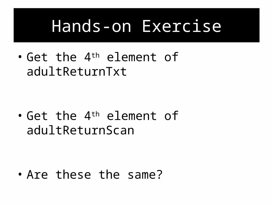
Hands-on Exercise

• Get the 4th element of adultReturnTxt

• Get the 4th element of adultReturnScan

• Are these the same?

Making a data frame from list

> adultReturnScan.df <- data.frame(

+ dam= adultReturnScan[[1]],

+ End.Date= adultReturnScan[[2]],

+ year= adultReturnScan[[3]],

+ Run=adultReturnScan[[4]],

+ Adult= as.numeric(adultReturnScan[[5]]),

+ Jack = as.numeric(adultReturnScan[[6]]))

> adultReturnScan.df

Subsetting Data Frames

> adultReturn[1:6,]

Same as:

> head(adultReturn)

Subsetting Data Frames

Look at column names:

> names(adultReturn)[1] "Dam" "End.Date" "year" "Run" "Adult" "Jack“

Look at all of Adult column

> adultReturn$Adult

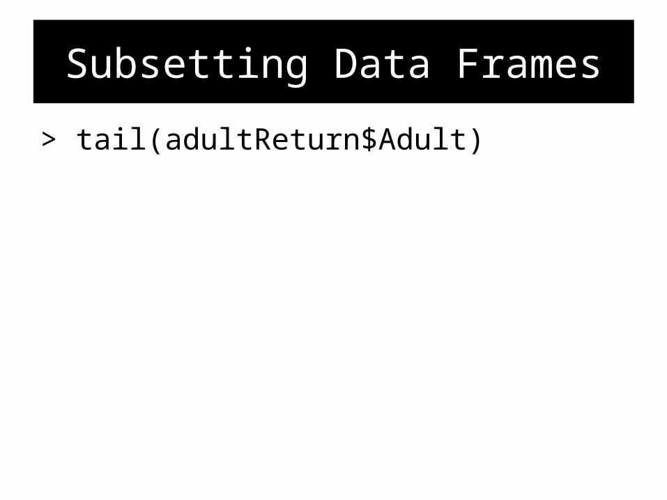
Subsetting Data Frames

> tail(adultReturn$Adult)

Same as:

> lenData <- length(adultReturn$Adult)> lenData1 <- dim(adultReturn)[1]

> lenData == lenData1

> adultReturn$Adult[(lenData-6):

+ lenData]

Subsetting Data Frames

Select only observations at Bonneville Dam:

> adultReturnBon <-

+ adultReturn[adultReturn$Dam ==

+ “BON”,]

Hands-on Exercises

• Make a new data frame called adultReturn2007 that only has observations from 2007, and adultReturn2008 that only has observations from 2008.

• Then do this again, but remove the column End.date when you do it.

• Plot Adult versus Juvenile for 2008 (use plot)

• Plot Adult in 2008 versus Adult in 2007

Add a row to a data frame: rbind

> adultReturn1 <- rbind(adultReturn,

+ c(“FSH”,”31-Oct”,2007,”summer”,

+ 12345,9876))

Warning message:In `[<-.factor`(`*tmp*`, ri, value = "FSH") : invalid factor level, NAs generated

Factors

• What is a factor:

– Categorical data (Nominal)

– Ordered data (Ordinal)

• Factors have many uses:

– ANOVA and other categorical analyses

– Creating groups for graphs

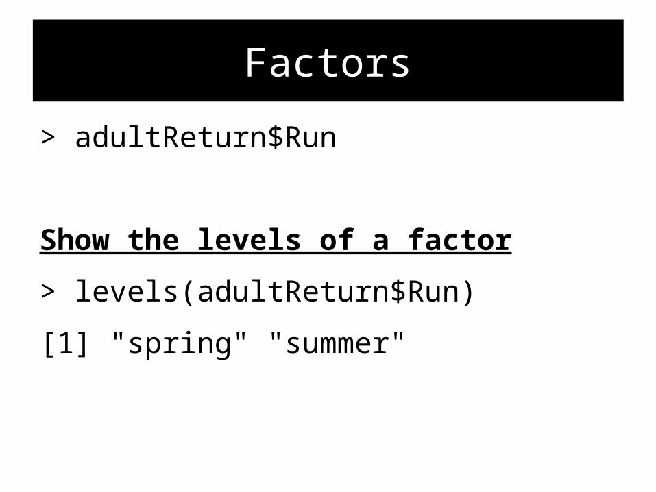
Factors

> adultReturn$Run

Show the levels of a factor

> levels(adultReturn$Run)

[1] "spring" "summer"

Factors

Change the order of levels in gender> adultReturn$Run <-

+ factor(adultReturn$Run,

+ levels= c("summer", "spring"))

> adultReturn$Run

Factors

Make a column not a factor> adultReturn$Run <-

+ as.character(adultReturn$Run)

> adultReturn$Run

Note that there are now no levels

Checking for factors

• To find out if something is a factor, ask the question:

> is.factor(adultReturn$Run)

[1] FALSE

> is.factor(adultReturn$Dam)

[1] TRUE

Analyzing All Columns at Once

Use sapply to analyze all columns each separately

> ?sapply

> sapply(adultReturn, FUN = is.factor)

Dam End.Date year Run Adult Jack

TRUE TRUE FALSE FALSE FALSE FALSE

Factors

• But, I prefer to do my data manipulations without factors, then make data into factors at the time of analysis or graphing

Reading Data into R Factorless

Look at help again:

> ?read.table

stringsAsFactors logical: should character vectors be converted to factors? Note that this is overridden by as.is and colClasses, both of which allow finer control.

> adultReturn <-

+ read.csv(“chinook_adult_return_data.csv”,

+ header = T, stringsAsFactors = F)

Making Factors

> runFact <-

+ as.factor(adultReturn$Run)

as.factor makes characters or numbers into factors

Hands-on Exercise

• Make a new object called yearFact that is the column year as a factor

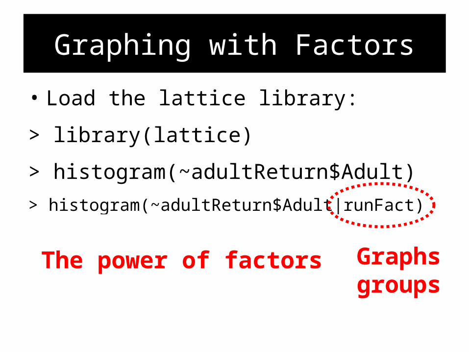
Graphing with Factors

• Load the lattice library:

> library(lattice)

> histogram(~adultReturn$Adult)

> histogram(~adultReturn$Adult|runFact)

> histogram(~adultReturn$Adult|

+ runFact*yearFact)

Graphs groups of groups

Graphs groups

The power of factors

Calculating Column Means

> mean(adultReturn$Adult)

[1] NA

Look up help for mean

> ?mean

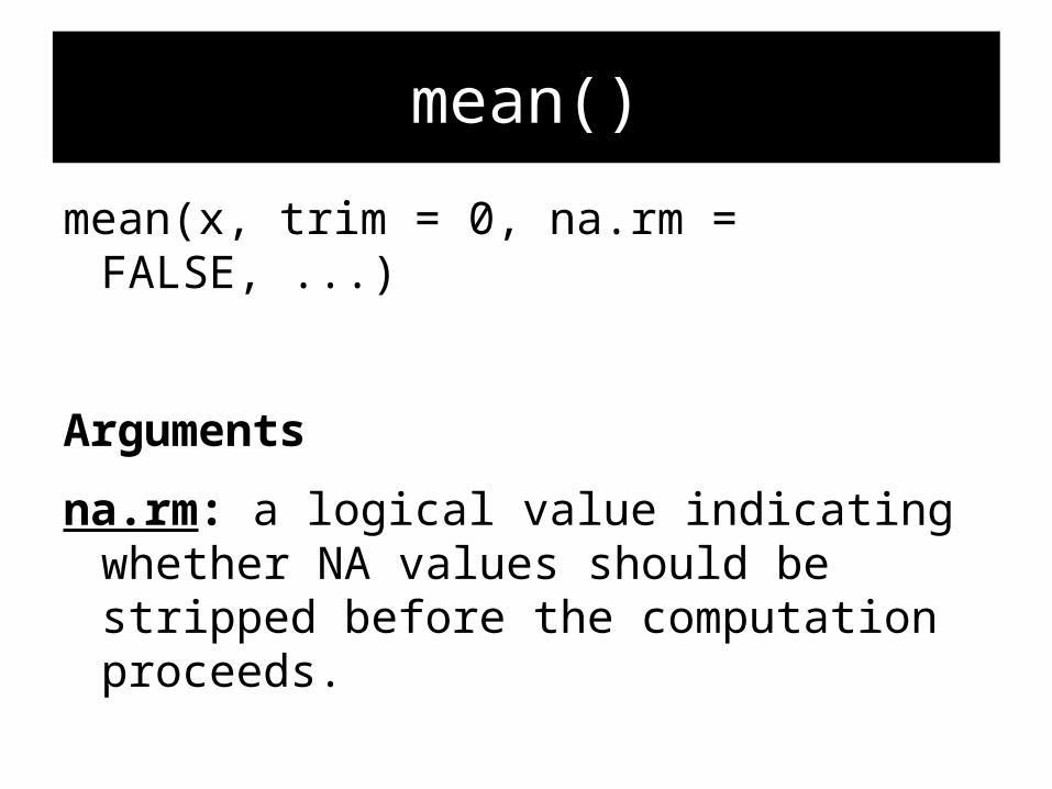
mean()

mean(x, trim = 0, na.rm = FALSE, ...)

Arguments

na.rm: a logical value indicating whether NA values should be stripped before the computation proceeds.

Calculating Column Means

> mean(adultReturn$Adult, na.rm = T)

[1] 33489.71

Hands-on Exercise

• Calculate the mean for the Jack column

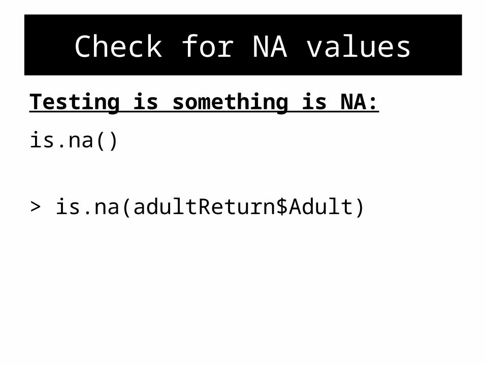
Check for NA values

Testing is something is NA:

is.na()

> is.na(adultReturn$Adult)

Check for NA values

Ask if any of the values are NA:

> any(is.na(adultReturn$Adult))

Ask if all of the values are NA:

> all(is.na(adultReturn$Adult))

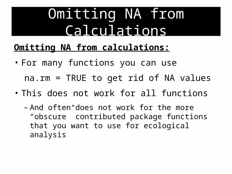
Omitting NA from Calculations

Omitting NA from calculations:

• For many functions you can use

na.rm = TRUE to get rid of NA values

• This does not work for all functions

– And often does not work for the more “obscure” contributed package functions that you want to use for ecological analysis

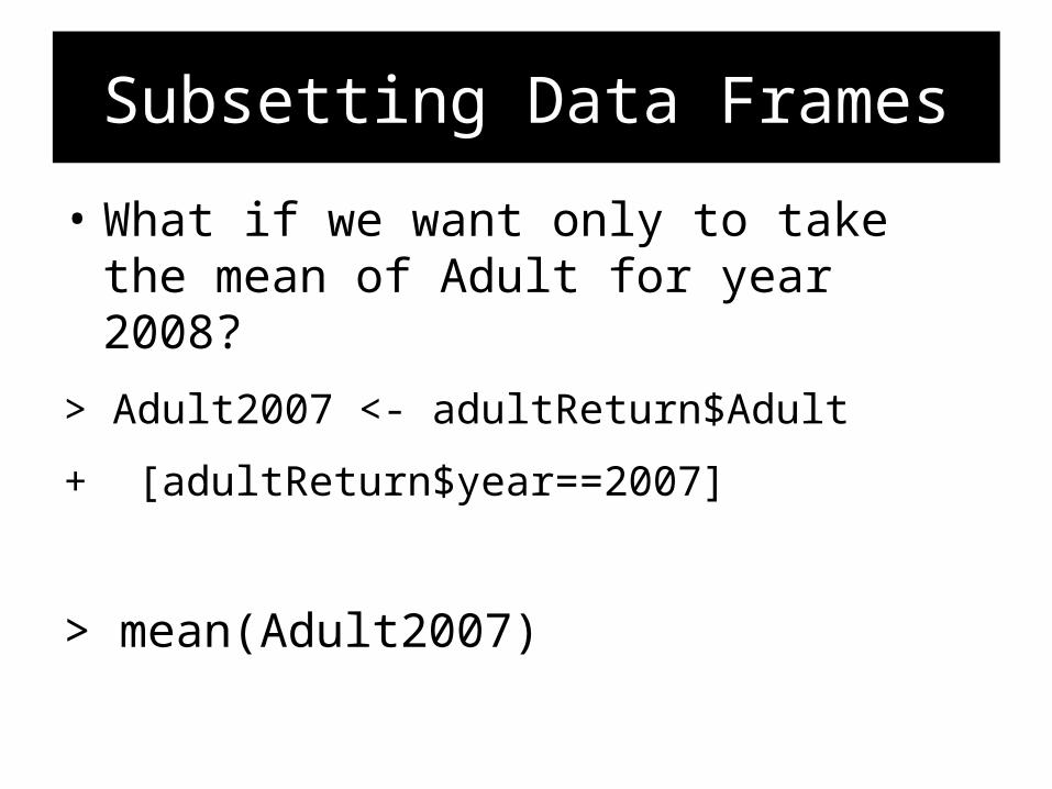
Subsetting Data Frames

• What if we want only to take the mean of Adult for year 2008?

> Adult2007 <- adultReturn$Adult

+ [adultReturn$year==2007]

> mean(Adult2007)

Subsetting Data Frames

• What if we want only to take the mean of Adult for year 2008 and spring run?

> AdultSpring2007 <- adultReturn$Adult

+ [(adultReturn$year==2007) &

+ (adultReturn$Run==“spring”)]

> mean(AdultSpring2007)

Hands-on Exercise

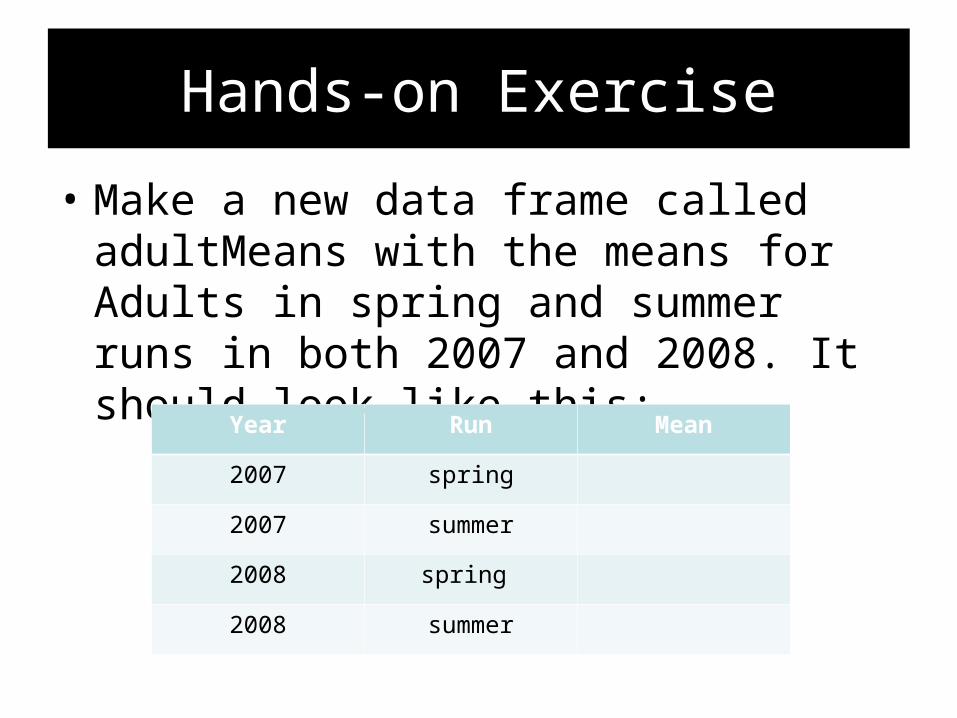
• Make a new data frame called adultMeans with the means for Adults in spring and summer runs in both 2007 and 2008. It should look like this:

Year Run Mean

2007 spring

2007 summer

2008 spring

2008 summer

Hands-on Exercise

• Find the command to write a table to a .csv file.

• Now, write the data frame you just created (adultMeans) to a file called adultMeans.csv

• Open this file up in Excel

Advanced Topics

• Aggregate

• Stack/unstack

• Time series objects

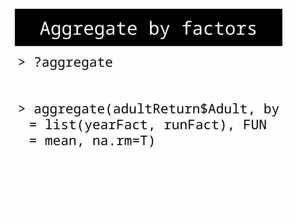
Aggregate by factors

> ?aggregate

> aggregate(adultReturn$Adult, by = list(yearFact, runFact), FUN = mean, na.rm=T)

Aggregation and Stacking

• stack(dataFrame)– turns an n by m data frame into an n*m by 2 data frame

• unstack(dataFrame, values~ind) turns an n*m by 2 data frame into an n by m data frame

Time Series

Create a time series numjobs

> numjobs <-

c(982,981,984,982,981,983,

983,983,983,979,973,979,

974,981,985,987,986,980,

983,983,988,994,990,999)

Time Series

Make numjobs a time series object:

> numjobs <- ts(numjobs,start=1995, frequency = 12)

Plot the time series:

> plot(numjobs)